K J E T I L S T O R E S L E T T E ND E P A R T M E N T O F E C O N O M I C S

U N I V E R S I T Y O F O S L OA P R I L 2 4 , 2 0 1 7

2

Why do we need multi-factor models? How are the multi-factor models grounded in the

CAPM/APT? What is the APT? How does the APT differ from the CAPM? How can we understand the Fama-French factor

models?

3

As a conceptual model, the CAPM is very useful. However, in practice, with the data and methods that are available to us to measure market beta, it is not sufficiently useful to compute required rates of return and expected returns or to discover mispriced securities.

Multifactor models are useful in this context. These models introduce uncertainty stemming from

multiple sources, whereas the CAPM, in principle, limits risk to one source – covariance with the market portfolio.

4 In the CAPM, the only relevant factor is the market model. However,

the market factor itself could be composed of different macroeconomic factors, e.g. business cycle uncertainty , interest rates, inflation etc.

Suppose the market is composed of two factors F1 and F2, i.e. Rm = sF1+ (1-s)F2, where even though we can’t observe Rm, we can observe F1and F2.

Then we can rewrite the CAPM as:E(Ri) = Rf + [Rm-Rf] = (1-)Rf + E(Rm) = (1-)Rf + [sE(F1) + (1-s)E(F2)]; rewriting, E(Ri) = Rf + s [E(F1) - Rf ]+ (1-s)[E(F2) - Rf].

This suggests a regression of Ri on (F1 - Rf ) and (F2 - Rf):E(Ri) = Rf + i1[E(F1)-Rf] + i2[E(F2)-Rf].

The two sources of risk here are exposure to the two factors; comparing the two equations, we also see that i1+i2=.

In this formulation, we don’t need to observe the market portfolio any more. (Although we would be able, in principle, to estimate s, and hence the market portfolio, as well.)

However all factors must be observable, and our market portfolio decomposition must be assumed to be correct.

5

The following description assumes two factors, but there could be many factors in principle.

Assume that returns can be generated as in a quasi-market model: Ri = ai + bi1F1 + bi2F2 + error. Note that we are no longer assuming any connection between these factors and the market portfolio.

If there are enough assets that are sufficiently different from each other, it should be possible to create three well-diversified portfolios that had no uncertainty other than their exposure to F1 and F2 (i.e. the error term would be zero).

Then, it will be true that the expected return on these three portfolios can be described by a linear combination of their b’s:E(R) = c0 + c1 bi1 + c2 bi2.

We can show this by means of an example.

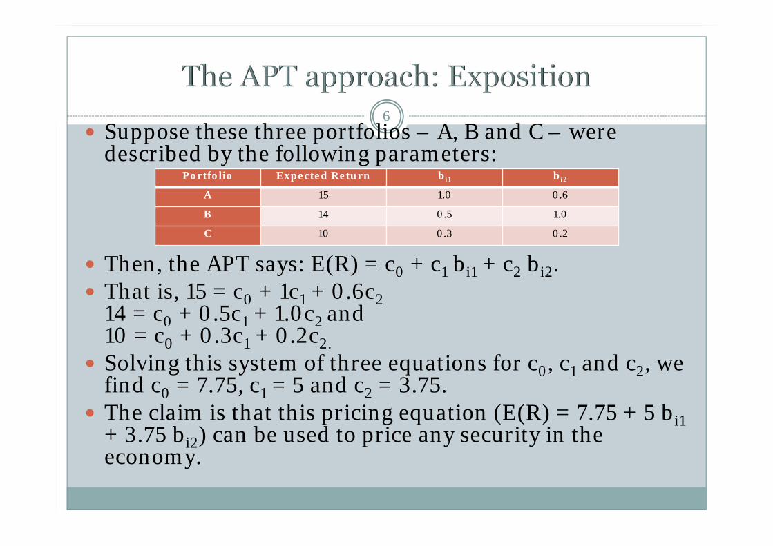
6 Suppose these three portfolios – A, B and C – were

described by the following parameters:

Then, the APT says: E(R) = c0 + c1 bi1 + c2 bi2. That is, 15 = c0 + 1c1 + 0.6c2

14 = c0 + 0.5c1 + 1.0c2 and 10 = c0 + 0.3c1 + 0.2c2.

Solving this system of three equations for c0, c1 and c2, we find c0 = 7.75, c1 = 5 and c2 = 3.75.

The claim is that this pricing equation (E(R) = 7.75 + 5 bi1+ 3.75 bi2) can be used to price any security in the economy.

Portfolio Expected Return bi1 bi2

A 15 1.0 0.6

B 14 0.5 1.0

C 10 0.3 0.2

7 Suppose a security, D, exists with bi1 = 0.6 and bi2 = 0.6. Since we have

enough securities, we can create a diversified portfolio with almost no idiosyncratic error that would also have the same values for bi1 and bi2. So let’s assume that our security has no idiosyncratic error.

Then, according to our equation, its expected return should be 7.75 + 5 (0.6) + 3.75 (0.6) = 13%. Suppose, however, that the expected return for D is 15%.

Then we can create a combination of securities A, B and C such that this new portfolio, E, has the same b-values as D.

This can be done by solving the system of equations: x1(1.0) + x2(0.5) + x3(0.3) = 0.6; x1(0.6) + x2(1.0) + x3(0.2) = 0.6; x1+x2+x3=1, where the xis are the portfolio weights for portfolio E. In this case, the solution is x1=x2=x3=1/3. This portfolio would have the same b-values as D, but would have an expected return of (15+14+10)/3 = 13%.

Hence an arbitrage opportunity exists. In general, the exercise of such arbitrage opportunities will force all

security prices to be such that expected returns are described by our single pricing equation, E(R) = c0 + c1 bi1 + c2 bi2.

8 We now simplify this pricing equation by identifying c0,

c1 and c2. Note that a portfolio with no b-risk will have to earn c0;

hence c0 = the risk-free rate. A portfolio with b1 risk equal to 1 and no b2 risk will earn

c0 + c1. Similarly, a portfolio with b2=1 and b1=0 will earn c0+c2.

Hence our pricing equation becomes: E(R) = Rf + [E(RF1)-Rf]bi1 + [E(RF2)-Rf]bi2, where E(RF1) is the expected return on a security or portfolio that has b1=1, b2=0, and E(RF2) is the expected return on a security/portfolio that has b1=0, b2=1.

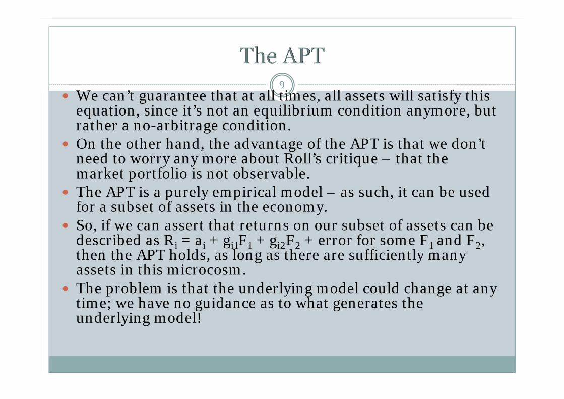
9 We can’t guarantee that at all times, all assets will satisfy this

equation, since it’s not an equilibrium condition anymore, but rather a no-arbitrage condition.

On the other hand, the advantage of the APT is that we don’t need to worry any more about Roll’s critique – that the market portfolio is not observable.

The APT is a purely empirical model – as such, it can be used for a subset of assets in the economy.

So, if we can assert that returns on our subset of assets can be described as Ri = ai + gi1F1 + gi2F2 + error for some F1 and F2, then the APT holds, as long as there are sufficiently many assets in this microcosm.

The problem is that the underlying model could change at any time; we have no guidance as to what generates the underlying model!

10

APT If the APT holds, then

there will be no arbitrage opportunities.

APT pricing relationship is quickly restored even if only a few investors recognize an arbitrage opportunity.

The expected return–beta relationship can be derived without using the true market portfolio.

CAPM Model is based on an

inherently unobservable “market” portfolio.

Rests on mean-variance efficiency. The actions of many small investors restore CAPM equilibrium.

CAPM describes equilibrium for all assets.

11

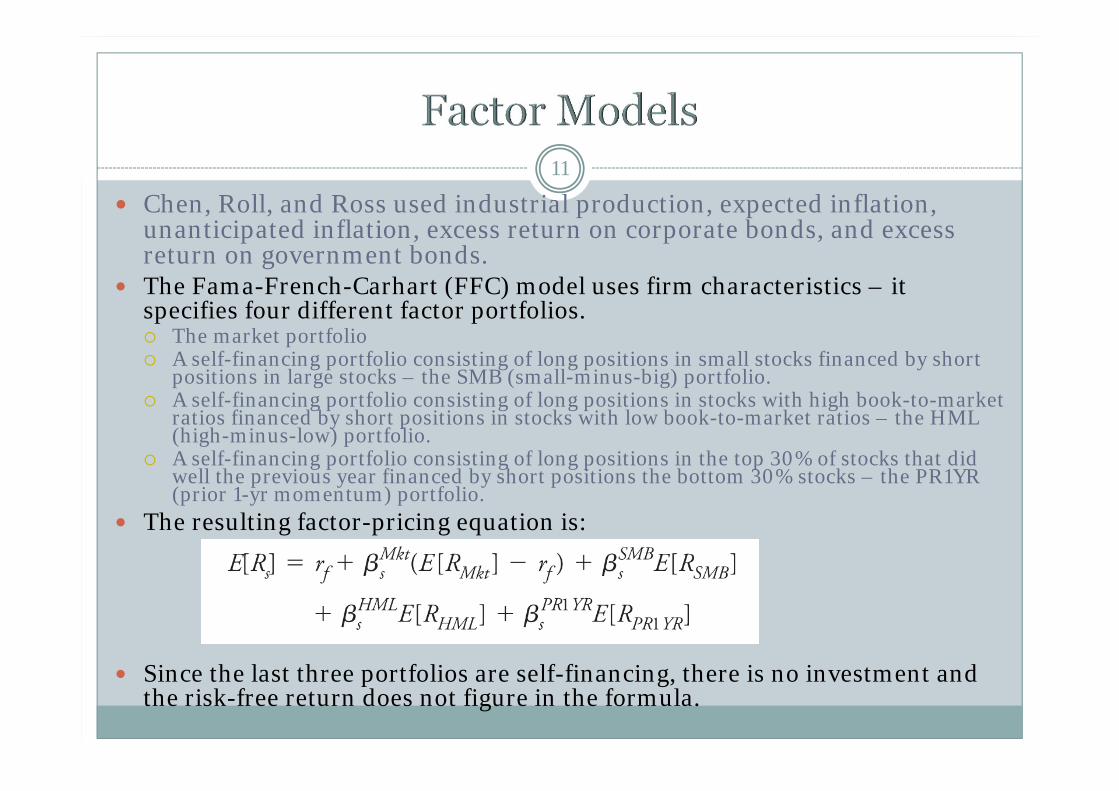
Chen, Roll, and Ross used industrial production, expected inflation, unanticipated inflation, excess return on corporate bonds, and excess return on government bonds.

The Fama-French-Carhart (FFC) model uses firm characteristics – it specifies four different factor portfolios. The market portfolio A self-financing portfolio consisting of long positions in small stocks financed by short

positions in large stocks – the SMB (small-minus-big) portfolio. A self-financing portfolio consisting of long positions in stocks with high book-to-market

ratios financed by short positions in stocks with low book-to-market ratios – the HML (high-minus-low) portfolio.

A self-financing portfolio consisting of long positions in the top 30% of stocks that did well the previous year financed by short positions the bottom 30% stocks – the PR1YR (prior 1-yr momentum) portfolio.

The resulting factor-pricing equation is:

Since the last three portfolios are self-financing, there is no investment and the risk-free return does not figure in the formula.

12

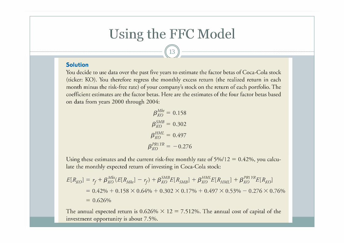
We see above estimates of expected risk premiums for the four FFC factors.

Let us now consider how to use the FFC model in practice. Suppose you find yourself in the situation described below:

13

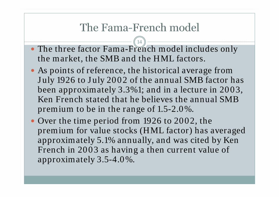
14 The three factor Fama-French model includes only

the market, the SMB and the HML factors. As points of reference, the historical average from

July 1926 to July 2002 of the annual SMB factor has been approximately 3.3%1; and in a lecture in 2003, Ken French stated that he believes the annual SMB premium to be in the range of 1.5-2.0%.

Over the time period from 1926 to 2002, the premium for value stocks (HML factor) has averaged approximately 5.1% annually, and was cited by Ken French in 2003 as having a then current value of approximately 3.5-4.0%.

15 We have seen that the CAPM could be true at the same time as

multi-factor models. The CAPM is not testable, in principle, because it requires the

observability of the market portfolio. Hence tests of the CAPM could “fail.” On the other hand, since the

factor pricing models, such as the Fama-French model or the Chen-Roll-Ross models are empirical, they could “succeed.”

But, as we saw, they could simply be multi-factor versions of an underlying CAPM.

Furthermore, some of the successes of alternative asset-pricing models could be spurious.

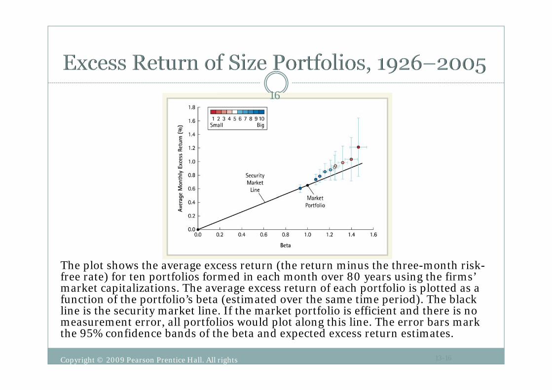
For example, the Fama-French model says that size is a proxy for risk. Some researchers (e.g. Banz) constructed portfolios of stocks and ordered them by the size of the stocks they contained and checked to see if all such portfolios lay on the Security Market Line.

They found that they did not – in fact, portfolios of small stocks tended, on average, to earn higher returns than portfolios of larger stocks.

Copyright © 2009 Pearson Prentice Hall. All rights reserved.

13-16

The plot shows the average excess return (the return minus the three-month risk-free rate) for ten portfolios formed in each month over 80 years using the firms’ market capitalizations. The average excess return of each portfolio is plotted as a function of the portfolio’s beta (estimated over the same time period). The black line is the security market line. If the market portfolio is efficient and there is no measurement error, all portfolios would plot along this line. The error bars mark the 95% confidence bands of the beta and expected excess return estimates.

16

17 Why should there be such a pattern? One answer is that it’s due to data-snooping – that is, given

enough characteristics, it will always be possible ex-post to find some characteristic that by pure chance happens to be correlated with the estimation error of average returns.

Another answer is that if the market portfolio is inefficient, then some assets would be overpriced and some assets would be underpriced. The overpriced assets would tend to be larger since their market values are larger than what they should be according to the CAPM. Similarly, underpriced assets would tend to be smaller. Since underpriced (overpriced) assets would tend over time to realize higher (lower) returns, we would expect to see patterns like those of Banz.

In fact, it turned out that portfolios consisting of stocks that had high book-to-market ratios (perhaps a proxy for underpriced stocks) had higher average returns than portfolios consisting of stocks with low book-to-market ratios.

Copyright © 2009 Pearson Prentice Hall. All rights reserved.

13-18

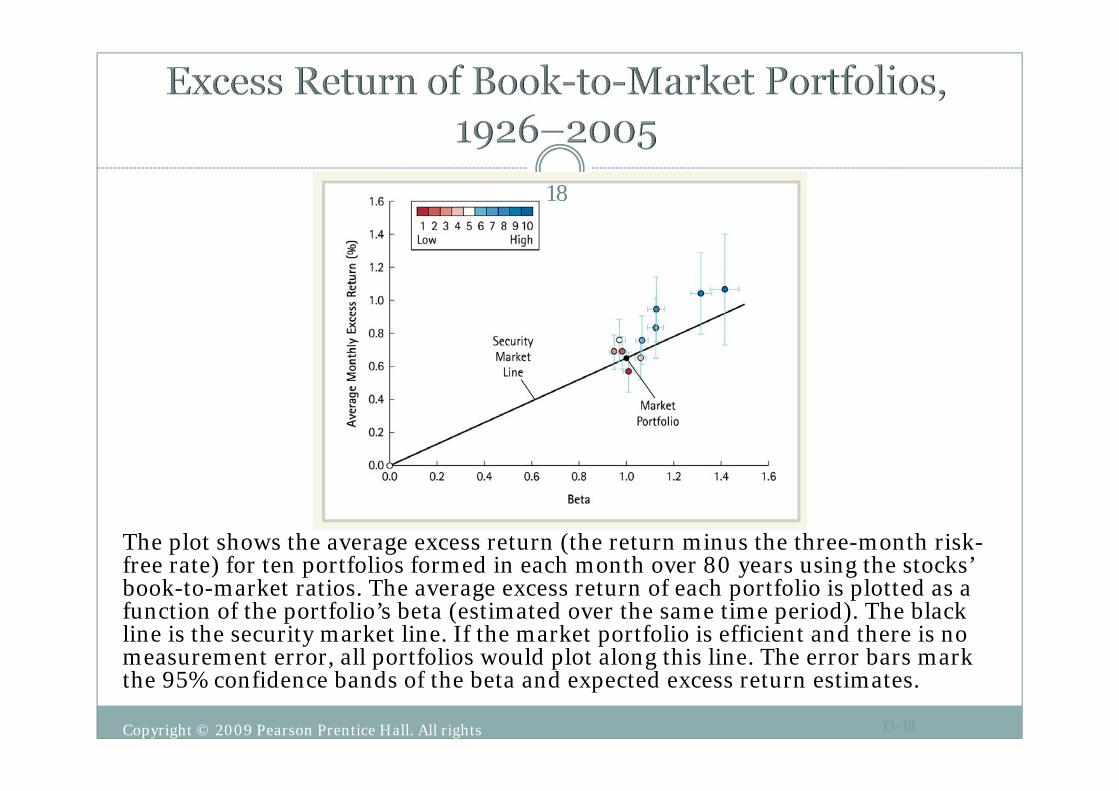
The plot shows the average excess return (the return minus the three-month risk-free rate) for ten portfolios formed in each month over 80 years using the stocks’ book-to-market ratios. The average excess return of each portfolio is plotted as a function of the portfolio’s beta (estimated over the same time period). The black line is the security market line. If the market portfolio is efficient and there is no measurement error, all portfolios would plot along this line. The error bars mark the 95% confidence bands of the beta and expected excess return estimates.

18

19

The second possibility is that the conventional tests of the CAPM fail because our proxy for the market portfolio leaves out important sources of risk.

When Jagannathan and Wang (1996) included proxies for business cycle risk and labor income risk (non-traded human capital), they found that both sources of risk were priced.

Our standard measures of beta assume constancy over the business cycle and our market portfolio leaves out human capital. Jagannathan and Wang’s model might be compensating for these risk sources.

20 One problem with the Fama-French model is that if we don’t know why assets

with high scores on their factors are rewarded, we won’t know when the model is no longer empirically valid (because we use historical data to test models); furthermore, we won’t be able to use the model to computer required rates on return on new assets or non-traded assets.

Liew and Vassalou (2000) show that returns on style portfolios (based on size or book-to-market factors) are positively related to future macroeconomic growth and hence may proxy business risk.

Petkova and Zhang (2005) also relate the higher average return on high book-to-market (value) portfolios to risk premiums.

Value firms have, on average, high amounts of tangible capital. Since such investment cannot be easily withdrawn, these firms are committed and hence at greater risk if there is an economic downturn; on the other hand, growth firms can defer investment more easily. As a result, it makes sense that such firms should earn higher average returns, as the Fama-French model says.

In fact, they find that the beta of the HML portfolio is negative in good economies, but positive in recessions. This means that the CAPM beta of value portfolios would be less than that of growth portfolios in good times, but higher in bad times. Thus, the HML beta is a kind of adjustment to the CAPM model that allows betas to vary across the business cycle, as in Jagannathanand Wang.

21

We have seen that sensitivity to momentum factors is also positively correlated with higher average returns; i.e. stocks that move in sync with market-wide momentum have higher average returns. Could this be related to liquidity?

One indicator of illiquidity is price reversals. Asset prices will dip when there are large sell orders, then recover.

Pastor and Stambaugh (2003) find that firms that have done well when market liquidity is high (high liquidity betas) have higher average returns. This is consistent with the notion that investors need more wealth when liquidity is lowest (e.g. to meet margin calls or to have funds for consumption without having to sell too many assets).

Although they weren’t able to link firm liquidity with market returns (because estimating individual stock liquidity requires much more data), the two notions are consistent with each other.

They also find that premiums to a momentum factor can mostly be accounted for by such liquidity premiums.

22 Unless we have an empirically successful asset pricing

model that is also theoretically meaningful, we have to be careful in using it.

To the extent that the risk premiums implied by the empirical model make sense, we can rely on it more.

The CAPM model, once its implementation is extended to take into account liquidity risks and non-traded human capital seems to be conceptually able to account for a lot of the empirical results. Note that, in theory, the CAPM includes human capital; however, in

practice, the measure of the market portfolio that is usually used excludes non-traded assets, such as human capital.

Above all, be cautious when using asset pricing models. Take into account risk due to model errors!