kite as a beam: a fast method to get the flying shape
TRANSCRIPT
HAL Id: hal-01804761https://hal-ensta-bretagne.archives-ouvertes.fr/hal-01804761
Submitted on 20 Jan 2020
HAL is a multi-disciplinary open accessarchive for the deposit and dissemination of sci-entific research documents, whether they are pub-lished or not. The documents may come fromteaching and research institutions in France orabroad, or from public or private research centers.
L’archive ouverte pluridisciplinaire HAL, estdestinée au dépôt et à la diffusion de documentsscientifiques de niveau recherche, publiés ou non,émanant des établissements d’enseignement et derecherche français ou étrangers, des laboratoirespublics ou privés.
Distributed under a Creative Commons Attribution| 4.0 International License
Kite as a beam: A fast method to get the flying shapeAlain de Solminihac, Alain Nême, Chloé Duport, Jean-Baptiste Leroux,
Kostia Roncin, Christian Jochum, Yves Parlier
To cite this version:Alain de Solminihac, Alain Nême, Chloé Duport, Jean-Baptiste Leroux, Kostia Roncin, et al.. Kiteas a beam: A fast method to get the flying shape. Airborne Wind Energy: Advances in Technol-ogy Development and Research, Springer, pp.79-97, 2018, Green Energy and Technology book series(GREEN), 978-981-10-1946-3. �10.1007/978-981-10-1947-0_4�. �hal-01804761�
Kite as a Beam: A Fast Method to get the Flying Shape
Alain de Solminihac, Alain Nême, Chloé Duport, Jean-Baptiste Leroux, Kostia
Roncin, Christian Jochum and Yves Parlier
Abstract Designing new large kite wings requires engineering tools that can ac-
count for flow-structure interaction. Although a fully coupled simulation of de-
formable membrane structures under aerodynamic load is already possible using Fi-
nite Element and Computational Fluid Dynamics methods this approach is compu-
tationally demanding. The core idea of the present study is to approximate a leading
edge inflatable tube kite by an assembly of equivalent beam elements. In spanwise
direction the wing is partitioned into several elementary cells, each consisting of a
leading edge segment, two lateral inflatable battens, and the corresponding portion
of canopy. The mechanical properties of an elementary cell—axial, transverse shear,
bending, and torsion stiffness—and the chordwise centroid position are determined
from the response to several imposed elementary displacements at its boundary, in
the case of a cell under an uniform pressure loading. For this purpose the cells are
supported at their four corners and different non-linear finite element analyses and
linear perturbation computations are carried out. The complete kite is represented
as an assembly of equivalent beams connected with rigid bodies. Coupled with a 3D
non-linear lifting line method to determine the aerodynamics this structural model
should allow predicting the flying shape and performance of new wing designs.
Alain de Solminihac · Alain Nême (�) · Chloé Duport · Jean-Baptiste Leroux · Kostia Roncin ·Christian Jochum
ENSTA Bretagne, FRE CNRS 3744, IRDL, 29200 Brest, France
e-mail: [email protected]
Yves Parlier
Beyond the sea, 1010 avenue de l’Europe, 33260 La Teste de Buch, France
e-mail: [email protected]
1
4.1 Introduction
The aim of this research project is the development of tethered kite systems as aux-
iliary devices for the propulsion of merchant ships. It is part of the beyond the sea R©
program which is lead by the Institut de Recherche Dupuy de Lôme (IRDL) of EN-
STA Bretagne. The goal is to design leading edge inflatable tube kites with surface
area larger than 300 m2. This requires a significant upscaling of common sports
kites which generally do not exceed a surface area of 30 m2. This upscaling process
raises several issues: What are the relevant physical effects to take into account? Is
it possible to use the same materials as for sports kites? Which geometry should the
bridle system have?
Point mass and rigid body models have been used for real-time or faster-than-
real-time simulation of the kite dynamics [7, 9]. A typical application of these
type of models is control engineering or flight path optimization. However, to get
a deeper understanding of the steering behavior and aerodynamic performance of
a highly flexible wing the shape deformation plays a crucial role. Breukels [3, 4]
developed an engineering model of a deformable flying kite, discretizing the tubular
frame by chains of rigid bodies connected by rotational springs and the canopy by
arrays of elastic springs and damper elements. All mechanical properties were de-
rived from basic experiments and the aerodynamic load distribution was prescribed
by an empirically determined correlation framework. The approach allows modeling
of aeroelastic effects.
Bosch [2] applied a geometrically non-linear finite element framework to the kite,
discretizing the tubular frame by beam elements and the canopy by custom-made
shell elements. This model was used to determine the quasi-static deformation re-
sulting from changes in the boundary conditions, such as aerodynamic loading and
steering line displacements. However, only macro-scale Fluid-Structure Interaction
(FSI) effects of spanwise torsion and bending of the wings were taken into account.
Gaunaa [8] developed a computationally efficient method for determining the aero-
dynamic performance of kites. The approach iteratively couples a Vortex Lattice
Method (VLM) with 2D airfoil data to account for the effects of airfoil thickness
and of viscosity. Deformation of the wing is not considered.
The aim of the present study is to develop an engineering tool which enables
kite designers to efficiently determine the flying shape of new kites. Given a few
design parameters such as the global wing shape, the material used and the wind
conditions, it should be possible to predict the flying shape and aerodynamic per-
formance. Structural non-linearity and macro-scale FSI calculations are conducted
as major influence factors. Contrary to the point mass and rigid body approaches,
the proposed method underlines the importance of considering the inflatable kite
as a deformable membrane structure. The method can be used to identify critical
aerodynamic peak loads and to take design measures to alleviate these.
In Sect. 4.2 and 4.3 the wing design and basic methods are first outlined, intro-
ducing the dicretization concept of the elementary cell, then followed by the identifi-
cation of mechanical and inertial properties and the assembly of several elementary
cells into a model of the complete wing. In Sect. 4.4 and 4.5 results are presented,
2
discussed and interpreted, elaborating also on the fast potential flow-based method
used to derive the instantaneous aerodynamic loading of the wing. The preliminary
content of the present chapter has been presented at the Airborne Wind Energy Con-
ference 2015 [17].
4.2 General Design Parameters
In this section the general problem definition is outlined. The kite design is devel-
oped in several steps starting from a 3D baseline. The required material properties
are then discussed, followed by a specification how the aerodynamic loading is de-
termined for different operational modes of the kite.
4.2.1 Design Geometry
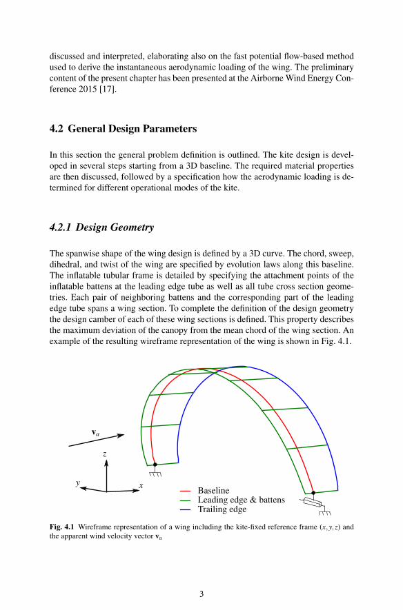
The spanwise shape of the wing design is defined by a 3D curve. The chord, sweep,
dihedral, and twist of the wing are specified by evolution laws along this baseline.
The inflatable tubular frame is detailed by specifying the attachment points of the
inflatable battens at the leading edge tube as well as all tube cross section geome-
tries. Each pair of neighboring battens and the corresponding part of the leading
edge tube spans a wing section. To complete the definition of the design geometry
the design camber of each of these wing sections is defined. This property describes
the maximum deviation of the canopy from the mean chord of the wing section. An
example of the resulting wireframe representation of the wing is shown in Fig. 4.1.
Leading edge & battensBaseline
Trailing edge
x
z
y
va
Fig. 4.1 Wireframe representation of a wing including the kite-fixed reference frame (x,y,z) and
the apparent wind velocity vector va
3
4.2.2 Material Properties
The fabric mechanical properties for the inflatable beams and the canopy are defined
using some data per unit mass (J/kg) for specifying the specific Young’s modulus
Em, and some data per unit area (kg/m2) for specifying the fabric density µ . The
Poisson’s ratio ν of the fabric should also be specified. In this study only isotropic
materials are considered, but the present model could be extended in the case of
anisotropic materials.
4.2.3 Relative Wind Conditions
The relative flow conditions at the wing are defined by the apparent wind velocity
va = vw −vp −vk, (4.1)
with vw denoting the true wind velocity and vp the ship velocity, both known prop-
erties, and vk denoting the kite velocity relative to the ship.
Kites can be used in two different flight modes to generate a traction force for
towing ships. In static flight mode the kite has a fixed position with respect to the
ship and the apparent wind velocity can be readily calculated from Eq. (4.1) by
setting vk = 0. In dynamic flight mode the kite is operated perpendicularly to the
tether and the kite velocity is a variable. It is possible to use a simple dynamic flight
model, such as the zero mass model [6, 12–14], to calculate vk as a function of time
and to use this in Eq. (4.1) to derive the apparent wind velocity.
The model described further in the next section requires an a priori estimation
of the pressure loading of the canopy, because its geometrical stiffness must be
considered. From the apparent wind velocity, and given an estimate a priori of the
aerodynamic lift coefficient, this can be achieved by calculating
Pm =1
2ρCLv2
a , (4.2)
with ρ denoting the air density and CL the aerodynamic lift coefficient. Given the
relatively high lift-to-drag ratio of the wings involved, and given an approximate
pressure loading is only required, the effect of the aerodynamic drag coefficient is
neglected here.
4.3 Structural Model of the Wing
In this section the structural model of the wing is built up in steps, starting from
individual elementary cells which are assembled into a structural model of the entire
flexible wing.
4
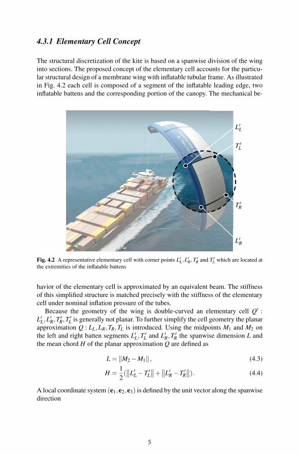
4.3.1 Elementary Cell Concept
The structural discretization of the kite is based on a spanwise division of the wing
into sections. The proposed concept of the elementary cell accounts for the particu-
lar structural design of a membrane wing with inflatable tubular frame. As illustrated
in Fig. 4.2 each cell is composed of a segment of the inflatable leading edge, two
inflatable battens and the corresponding portion of the canopy. The mechanical be-
Fig. 4.2 A representative elementary cell with corner points L′L,L
′R,T
′R and T ′
L which are located at
the extremities of the inflatable battens
havior of the elementary cell is approximated by an equivalent beam. The stiffness
of this simplified structure is matched precisely with the stiffness of the elementary
cell under nominal inflation pressure of the tubes.
Because the geometry of the wing is double-curved an elementary cell Q′ :
L′L,L
′R,T
′R,T
′L is generally not planar. To further simplify the cell geometry the planar
approximation Q : LL,LR,TR,TL is introduced. Using the midpoints M1 and M2 on
the left and right batten segments L′L,T
′L and L′
R,T′
R the spanwise dimension L and
the mean chord H of the planar approximation Q are defined as
L = ‖M2 −M1‖ , (4.3)
H =1
2(∥
∥L′L −T ′
L
∥
∥+∥
∥L′R −T ′
R
∥
∥). (4.4)
A local coordinate system (e1,e2,e3) is defined by the unit vector along the spanwise
direction
L′
L
T′
L
T′
R
L′
R
5
e1 =1
L(M2 −M1), (4.5)
the unit vector perpendicular to the plane
e3 =(T ′
R −L′L)× (T ′
L −L′R)
‖(T ′R −L′
L)× (T ′L −L′
R)‖, (4.6)
and a third unit vector defined as cross product
e2 = e3 × e1. (4.7)
4.3.2 Equivalent Beam Concept
The equivalent beam is introduced to describe the mechanical behavior of the ele-
mentary cell by means of an idealized structural object. The following beam proper-
ties are identified on the basis of finite element analysis of the elementary cell under
various loads:
• Beam centroid distance from the leading edge,
• Tension/Compression stiffness,
• Bending stiffness,
• Torsion stiffness,
• Shear coefficients.
The structural analysis is performed with the finite element solver AbaqusTM
.
4.3.3 Finite Element Model of the Elementary Cell
As a conclusion of a convergence analysis the canopy of the elementary cell is dis-
cretized by 2000 rectangular linear membrane elements. The mechanical properties
used for the canopy are the in-plane stiffness EC = µCEm,C and the Poisson ratio
νC. The subscript C indicates properties of the canopy. It is possible to adapt these
mechanical properties for the different regions of the canopy, as for instance at the
trailing edge if canopy reinforcement effects have to be investigated.
The canopy of the elementary cell is supported by the leading edge tube and two
battens. These inflatable elements are modeled as straight beams and discretized by
200 linear beam elements in total for three tubes. Starting from the known beam
radius R, fabric stiffness EB = µBEm,B and Poisson ratio νB, where subscript B indi-
cates properties of the beam, the section properties are estimated as:
• Elongation stiffness: 2πREB,
• Bending stiffness: πR3EB,
• Transverse shear stiffness [5] :0.53
1+νB
πREB,
6
• Torsion stiffness: π
1+νB
R3EB.
Because in the final wing model the elementary cells are connected the stiffness of
the finite element beam representing a batten is only 50% of the stiffness of the full
batten. Underlying is a linear superposition assumption. In this study, it is assumed
that the kite design geometry allows to consider the tips of the wing as battens. For
these, the stiffness of the corresponding finite element beam is 100% of the stiffness
of the full batten.
4.3.4 Pressurization of the Elementary Cell
The geometrical stiffness of the canopy must be considered because it is comparable
to the stiffness of the beam frame. The initial shape of the canopy before applying
the pressure loading is expressed in the Cartesian frame (e1,e2,e3) with origin at LL
x = x1e1 + x2e2 + x3e3, (4.8)
with x3 given by the following analytic expression
x3 = λH sin(
πx1
L
)
sin(
πx2
H
)
(4.9)
and λ denoting the design camber of the canopy with a value of λ ≈ 5%.
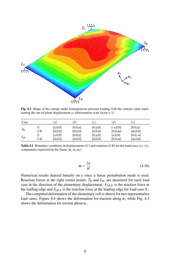
The first computation step is a non-linear geometrical analysis. The four cor-
ners (TL,LL,LR,TR) are clamped in space and the elementary cell is loaded with the
estimated homogeneous pressure as described in Sect. 4.2.3.
Since membrane elements have no bending stiffness, a damping factor of 5×10⁶
is introduced in the AbaqusTM
simulation [16] to achieve convergence of the nodal
force balance at the end of the time step (100 seconds). Then a second computation
step is conducted without damping to check the validity of the obtained solution. A
representative simulation result is shown in Fig. 4.3. As a last step the characteristics
of the elementary cell under homogeneous pressure loading are determined.
4.3.5 Computation in Linear Perturbation Mode
Starting from this pressurized structure, five linear perturbation calculation cases
are completed in order to evaluate the stiffnesses of the elementary cell with respect
to the different global degrees of freedom. The cases are listed in Table 4.1 where
(a) represents traction along e1, (b) out-of-plane shear along e3, (c) in-plane shear
along e2, (d) in-plane bending about e3 and (e) torsion about e1. The elementary
displacement is given by a and ω is determined by
7
e1
e2
e3
TR
TL
LR
LL
Fig. 4.3 Shape of the canopy under homogeneous pressure loading with the contour value repre-
senting the out-of-plane displacement x3 (deformation scale factor = 1)
Case (a) (b) (c) (d) (e)
TRU [a,0,0] [0,0,a] [0,a,0] [-a,0,0] [0,0,a]
UR [0,0,0] [0,0,0] [0,0,0] [0,0,ω] [ω ,0,0]
LRU [a,0,0] [0,0,a] [0,a,0] [a,0,0] [0,0,-a]
UR [0,0,0] [0,0,0] [0,0,0] [0,0,ω] [ω ,0,0]
Table 4.1 Boundary conditions in displacements (U) and rotations (UR) for the load cases (a)–(e),components expressed in the frame (e1,e2,e3)
ω =2a
H. (4.10)
Numerical results depend linearly on a since a linear perturbation mode is used.
Reaction forces at the right corner points, TR and LR, are measured for each load
case in the direction of the elementary displacement. FT R,X is the reaction force at
the trailing edge and FLR,X is the reaction force at the leading edge for load case X .
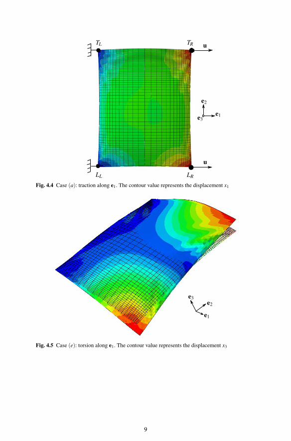
The computed deformation of the elementary cell is shown for two representative
load cases. Figure 4.4 shows the deformation for traction along e1 while Fig. 4.5
shows the deformation for torsion about e1.
8
e1
e2
e3
TRTL
LRLL
u
u
Fig. 4.4 Case (a): traction along e1. The contour value represents the displacement x1
e1
e2
e3
Fig. 4.5 Case (e): torsion along e1. The contour value represents the displacement x3
9
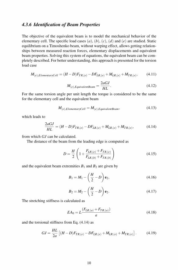
4.3.6 Identification of Beam Properties
The objective of the equivalent beam is to model the mechanical behavior of the
elementary cell. The specific load cases (a), (b), (c), (d) and (e) are studied. Static
equilibrium on a Timoshenko beam, without warping effect, allows getting relation-
ships between measured reaction forces, elementary displacements and equivalent
beam properties. Solving this system of equations, the equivalent beam can be com-
pletely described. For better understanding, this approach is presented for the torsion
load case
M(e),ElementaryCell = (H −D)FT R,(e)−DFLR,(e)+MLR,(e)+MT R,(e), (4.11)
M(e),EquivalentBeam =2aGJ
HL. (4.12)
For the same torsion angle per unit length the torque is considered to be the same
for the elementary cell and the equivalent beam
M(e),ElementaryCell = M(e),EquivalentBeam, (4.13)
which leads to
2aGJ
HL= (H −D)FT R,(e)−DFLR,(e)+MLR,(e)+MT R,(e), (4.14)
from which GJ can be calculated.
The distance of the beam from the leading edge is computed as
D =H
2
(
1+FLR,(e)+FT R,(e)
FLR,(b)+FT R,(b)
)
(4.15)
and the equivalent beam extremities B1 and B2 are given by
B1 = M1 −
(
H
2−D
)
e2, (4.16)
B2 = M2 −
(
H
2−D
)
e2. (4.17)
The stretching stiffness is calculated as
EA0 = L(FLR,(a)+FT R,(a))
a(4.18)
and the torsional stiffness from Eq. (4.14) as
GJ =HL
2a
[
(H −D)FT R,(e)−DFLR,(e)+MLR,(e)+MT R,(e)
]
. (4.19)
10
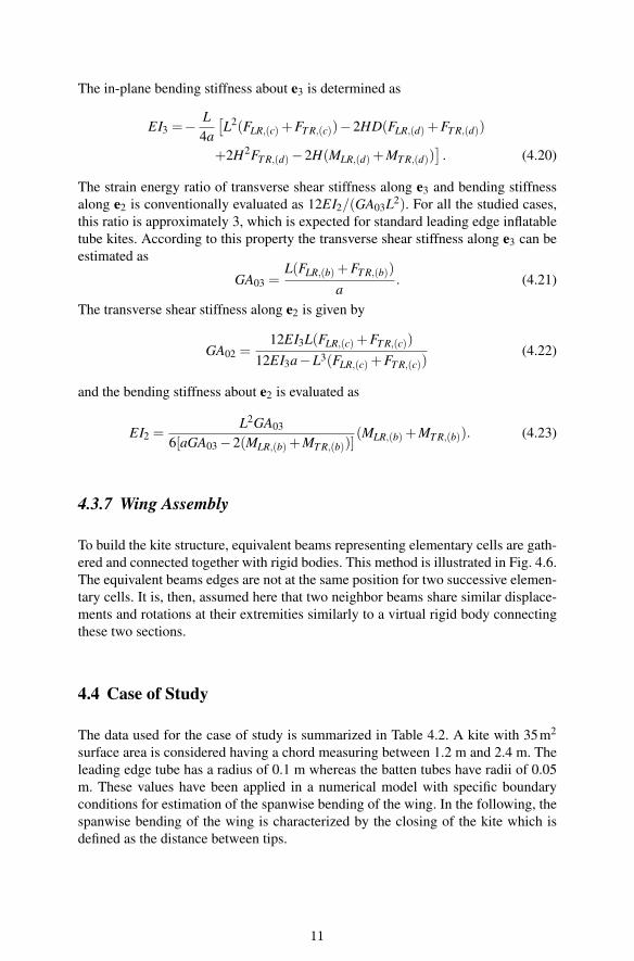
The in-plane bending stiffness about e3 is determined as
EI3 =−L
4a
[
L2(FLR,(c)+FT R,(c))−2HD(FLR,(d)+FT R,(d))
+2H2FT R,(d)−2H(MLR,(d)+MT R,(d))]
. (4.20)
The strain energy ratio of transverse shear stiffness along e3 and bending stiffness
along e2 is conventionally evaluated as 12EI2/(GA03L2). For all the studied cases,
this ratio is approximately 3, which is expected for standard leading edge inflatable
tube kites. According to this property the transverse shear stiffness along e3 can be
estimated as
GA03 =L(FLR,(b)+FT R,(b))
a. (4.21)
The transverse shear stiffness along e2 is given by
GA02 =12EI3L(FLR,(c)+FT R,(c))
12EI3a−L3(FLR,(c)+FT R,(c))(4.22)
and the bending stiffness about e2 is evaluated as
EI2 =L2GA03
6[aGA03 −2(MLR,(b)+MT R,(b))](MLR,(b)+MT R,(b)). (4.23)
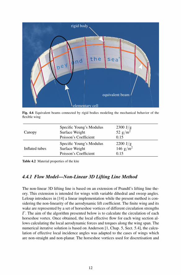
4.3.7 Wing Assembly
To build the kite structure, equivalent beams representing elementary cells are gath-
ered and connected together with rigid bodies. This method is illustrated in Fig. 4.6.
The equivalent beams edges are not at the same position for two successive elemen-
tary cells. It is, then, assumed here that two neighbor beams share similar displace-
ments and rotations at their extremities similarly to a virtual rigid body connecting
these two sections.
4.4 Case of Study
The data used for the case of study is summarized in Table 4.2. A kite with 35m2
surface area is considered having a chord measuring between 1.2 m and 2.4 m. The
leading edge tube has a radius of 0.1 m whereas the batten tubes have radii of 0.05
m. These values have been applied in a numerical model with specific boundary
conditions for estimation of the spanwise bending of the wing. In the following, the
spanwise bending of the wing is characterized by the closing of the kite which is
defined as the distance between tips.
11
rigid body
elementary cell
equivalent beam
Fig. 4.6 Equivalent beams connected by rigid bodies modeling the mechanical behavior of the
flexible wing
Canopy
Specific Young’s Modulus 2300 J/g
Surface Weight 52 g/m2
Poisson’s Coefficient 0.15
Inflated tubes
Specific Young’s Modulus 2200 J/g
Surface Weight 146 g/m2
Poisson’s Coefficient 0.15
Table 4.2 Material properties of the kite
4.4.1 Flow Model—Non-Linear 3D Lifting Line Method
The non-linear 3D lifting line is based on an extension of Prandtl’s lifting line the-
ory. This extension is intended for wings with variable dihedral and sweep angles.
Leloup introduces in [14] a linear implementation while the present method is con-
sidering the non-linearity of the aerodynamic lift coefficient. The finite wing and its
wake are represented by a set of horseshoe vortices of different circulation strengths
Γ . The aim of the algorithm presented below is to calculate the circulation of each
horseshoe vortex. Once obtained, the local effective flow for each wing section al-
lows calculating the local aerodynamic forces and torques along the wing span. The
numerical iterative solution is based on Anderson [1, Chap. 5, Sect. 5.4], the calcu-
lation of effective local incidence angles was adapted to the cases of wings which
are non-straight and non-planar. The horseshoe vortices used for discretisation and
12
calculation of their influences are derived from Katz and Plotkin [10, Chap. 12, Fig.
12.2 (a)].
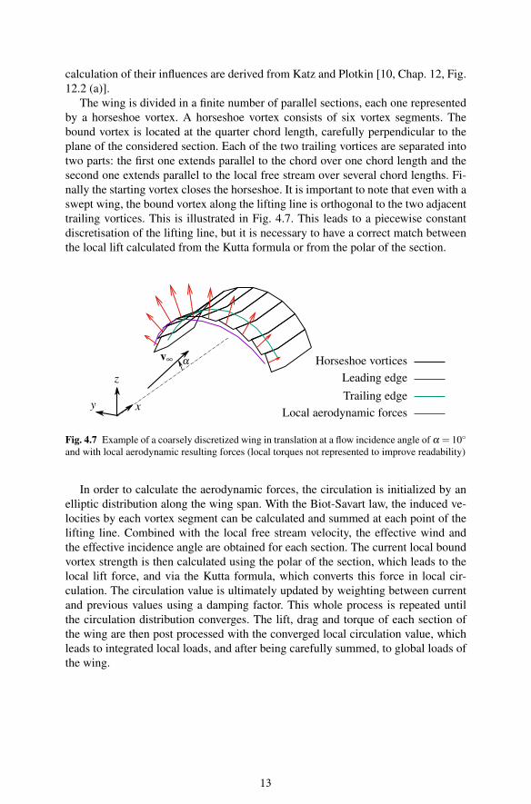
The wing is divided in a finite number of parallel sections, each one represented
by a horseshoe vortex. A horseshoe vortex consists of six vortex segments. The
bound vortex is located at the quarter chord length, carefully perpendicular to the
plane of the considered section. Each of the two trailing vortices are separated into
two parts: the first one extends parallel to the chord over one chord length and the
second one extends parallel to the local free stream over several chord lengths. Fi-
nally the starting vortex closes the horseshoe. It is important to note that even with a
swept wing, the bound vortex along the lifting line is orthogonal to the two adjacent
trailing vortices. This is illustrated in Fig. 4.7. This leads to a piecewise constant
discretisation of the lifting line, but it is necessary to have a correct match between
the local lift calculated from the Kutta formula or from the polar of the section.
Horseshoe vortices
Leading edge
Trailing edge
Local aerodynamic forcesx
z
y
v∞ α
Fig. 4.7 Example of a coarsely discretized wing in translation at a flow incidence angle of α = 10◦
and with local aerodynamic resulting forces (local torques not represented to improve readability)
In order to calculate the aerodynamic forces, the circulation is initialized by an
elliptic distribution along the wing span. With the Biot-Savart law, the induced ve-
locities by each vortex segment can be calculated and summed at each point of the
lifting line. Combined with the local free stream velocity, the effective wind and
the effective incidence angle are obtained for each section. The current local bound
vortex strength is then calculated using the polar of the section, which leads to the
local lift force, and via the Kutta formula, which converts this force in local cir-
culation. The circulation value is ultimately updated by weighting between current
and previous values using a damping factor. This whole process is repeated until
the circulation distribution converges. The lift, drag and torque of each section of
the wing are then post processed with the converged local circulation value, which
leads to integrated local loads, and after being carefully summed, to global loads of
the wing.
13
4.4.2 AbaqusTM
Procedure
The structural analysis is conducted using the commercial solver AbaqusTM
. The
computation of the equivalent beam deformation under aerodynamic loading is per-
formed with a large-displacement formulation from the initial configuration of the
equivalent beam which accounts for its stress-free geometry. The large-displacement
formulation of Timoshenko beam elements used in AbaqusTM
[16] is based on a mul-
tiplicative decomposition of the deformation gradient into a stretch part (Fs) and a
distorsion part (Fd). The strain tensor is obtained by addition of the logarithm of Fs
and the Green-Lagrange formula applied to Fd . No artificial damping forces were
introduced into the finite element model. Since the geometrical location of the finite
element beam lies on the lifting line, its local section direction n1 is determined
with the orthogonal projection of the point M, defined as the geometric center of
the beam element, on the equivalent beam which is located at the distance D (see
Eq. (4.15)) from the leading edge. If P represents the projection of M, it can be
determined from
P−B1 = [(M−B1) · e1]e1. (4.24)
If t stands for the unit vector along the beam element axis, the unit vector n1 is
obtained from⎧
⎨
⎩
n′1 = (P−M)− [(P−M) · t] t,
n1 =n′
1∥
∥n′1
∥
∥
.(4.25)
The second local section direction of the beam element n2 is such that
n2 = t×n1. (4.26)
We assume that the location of the beam element section centroid is expressed in
the local beam element frame (t,n1,n2) as
[0,∥
∥n′1
∥
∥ ,0]⊤. (4.27)
The beam element section properties are the same as in the Eqs. (4.18) to (4.23)
assuming the local beam element frame (t,n1,n2) is matching the equivalent beam
frame (e1,e2,e3).
4.4.3 Boundary and Wind Conditions
To model the closing and opening of the kite under load the specific boundary con-
ditions listed in Table 4.3 are chosen.
By definition the apparent wind velocity is aligned with the x-axis as illustrated in
Fig. 4.1. It has a value of 30 m/s at an air density of 1.2kg/m3. No twist is considered
for the stress-free geometry of the kite and the wind is parallel to its symmetry
14
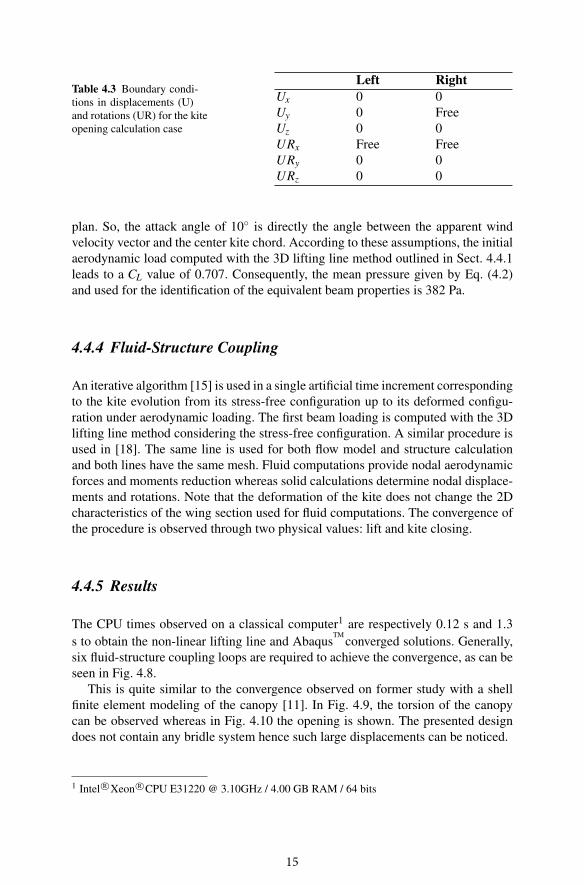
Table 4.3 Boundary condi-
tions in displacements (U)
and rotations (UR) for the kite
opening calculation case
Left Right
Ux 0 0
Uy 0 Free
Uz 0 0
URx Free Free
URy 0 0
URz 0 0
plan. So, the attack angle of 10◦ is directly the angle between the apparent wind
velocity vector and the center kite chord. According to these assumptions, the initial
aerodynamic load computed with the 3D lifting line method outlined in Sect. 4.4.1
leads to a CL value of 0.707. Consequently, the mean pressure given by Eq. (4.2)
and used for the identification of the equivalent beam properties is 382 Pa.
4.4.4 Fluid-Structure Coupling
An iterative algorithm [15] is used in a single artificial time increment corresponding
to the kite evolution from its stress-free configuration up to its deformed configu-
ration under aerodynamic loading. The first beam loading is computed with the 3D
lifting line method considering the stress-free configuration. A similar procedure is
used in [18]. The same line is used for both flow model and structure calculation
and both lines have the same mesh. Fluid computations provide nodal aerodynamic
forces and moments reduction whereas solid calculations determine nodal displace-
ments and rotations. Note that the deformation of the kite does not change the 2D
characteristics of the wing section used for fluid computations. The convergence of
the procedure is observed through two physical values: lift and kite closing.
4.4.5 Results
The CPU times observed on a classical computer1 are respectively 0.12 s and 1.3
s to obtain the non-linear lifting line and AbaqusTM
converged solutions. Generally,
six fluid-structure coupling loops are required to achieve the convergence, as can be
seen in Fig. 4.8.
This is quite similar to the convergence observed on former study with a shell
finite element modeling of the canopy [11]. In Fig. 4.9, the torsion of the canopy
can be observed whereas in Fig. 4.10 the opening is shown. The presented design
does not contain any bridle system hence such large displacements can be noticed.
1 Intel R©Xeon R©CPU E31220 @ 3.10GHz / 4.00 GB RAM / 64 bits
15
0 2 4 6 8 10 12
Iteration number [-]
0
3000
6000
9000
12000
15000
Lif
tfo
rce
[N]
0
1
2
3
4
5
Kit
ecl
osi
ng
[m]
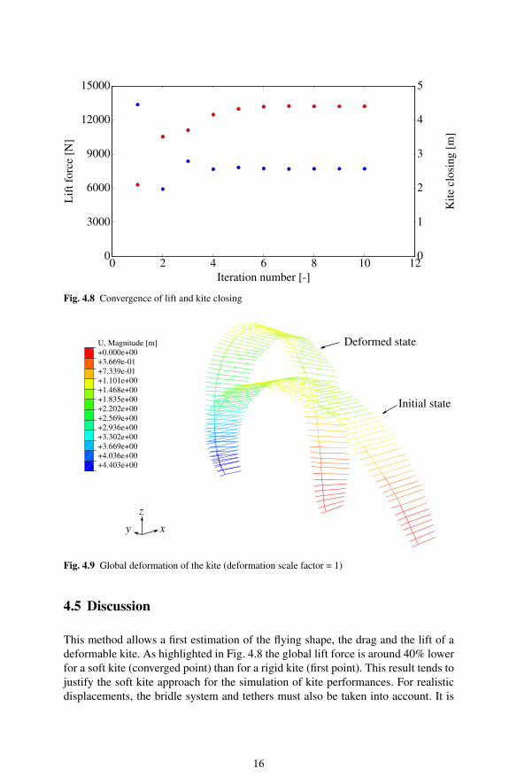
Fig. 4.8 Convergence of lift and kite closing
x
z
y
U, Magnitude [m]
+0.000e+00
+3.669e-01
+7.339e-01
+1.101e+00
+1.468e+00
+1.835e+00
+2.202e+00
+2.569e+00
+2.936e+00
+3.302e+00
+3.669e+00
+4.036e+00
+4.403e+00
Deformed state
Initial state
Fig. 4.9 Global deformation of the kite (deformation scale factor = 1)
4.5 Discussion
This method allows a first estimation of the flying shape, the drag and the lift of a
deformable kite. As highlighted in Fig. 4.8 the global lift force is around 40% lower
for a soft kite (converged point) than for a rigid kite (first point). This result tends to
justify the soft kite approach for the simulation of kite performances. For realistic
displacements, the bridle system and tethers must also be taken into account. It is
16
x
z
y
U, U2 [m]
+0.000e+00
+3.669e-01
+7.339e-01
+1.101e+00
+1.468e+00
+1.835e+00
+2.202e+00
+2.569e+00
+2.936e+00
+3.302e+00
+3.669e+00
+4.036e+00
Deformed state
Initial state
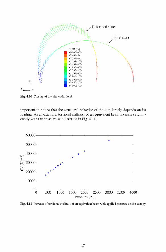
Fig. 4.10 Closing of the kite under load
important to notice that the structural behavior of the kite largely depends on its
loading. As an example, torsional stiffness of an equivalent beam increases signifi-
cantly with the pressure, as illustrated in Fig. 4.11.
0 500 1000 1500 2000 2500 3000 3500 4000
Pressure [Pa]
0
10000
20000
30000
40000
50000
60000
GJ
[N.m
2]
Fig. 4.11 Increase of torsional stiffness of an equivalent beam with applied pressure on the canopy
17
4.6 Conclusion
In this study the complex structural behavior of a soft kite was simplified to a simple
arrangement of beams. The parameters of the beams were calculated from finite
element analysis of so-called elementary cells, which model the canopy of a single
kite cell, under homogeneous pressure. This pressure was derived from the global
lift coefficient of the initial kite geometry.
Coupled with a fluid model, the simplified structure model approach presented
in this study allows a prediction of the flying shape and helps obtaining a better
understanding of the main phenomena which have to be considered. It is as well a
quick (a couple of minutes) and convenient way to get a first estimation of the kite
performance accounting for fluid-structure interaction.
However, the “kite as a beam” model has not been compared to more detailed
structural models. This analysis is currently ongoing. Additionally, the “kite as a
beam” approach presented here does not directly address local aspects like stresses
and strains in the canopy and in the inflatable structure. These aspects have to be in-
vestigated with fully coupled FEA / CFD computations. Overall validation requires
relevant experiments that are currently under progress at the institute.
The next step to extend the “kite as a beam” model would be the inclusion of
bridles and tethers to improve their design and for better towing force estimations.
In parallel, it will be necessary to develop a more realistic beam frame model for
the kite structure. A parametric formulation of the influence of the geometry of the
canopy on the kite stiffness will be developed. Hence, the stiffness of the elementary
cells will depend on the aerodynamic pressure. The new model should also enable an
improvement of the design of the inflatable leading edge and the battens according
to stress limit and buckling condition.
References
1. Anderson, J. D.: Fundamentals of Aerodynamics. 5th ed. McGraw-Hill (2014)
2. Bosch, A., Schmehl, R., Tiso, P., Rixen, D.: Dynamic nonlinear aeroelastic model of a kite
for power generation. AIAA Journal of Guidance, Control and Dynamics 37(5), 1426–1436
(2014). doi: 10.2514/1.G000545
3. Breukels, J.: An Engineering Methodology for Kite Design. Ph.D. Thesis, Delft University of
Technology, 2011. http://resolver.tudelft.nl/uuid:cdece38a-1f13-47cc-b277-ed64fdda7cdf
4. Breukels, J., Schmehl, R., Ockels, W.: Aeroelastic Simulation of Flexible Membrane Wings
based on Multibody System Dynamics. In: Ahrens, U., Diehl, M., Schmehl, R. (eds.) Air-
borne Wind Energy, Green Energy and Technology, Chap. 16, pp. 287–305. Springer, Berlin
Heidelberg (2013). doi: 10.1007/978-3-642-39965-7_16
5. Cowper, R. G.: The Shear Coefficient in Timoshenko’s Beam Theory. Journal of Applied
Mechanics 33(2), 335–340 (1966). doi: 10.1115/1.3625046
6. Dadd, G. M., Hudson, D. A., Shenoi, R. A.: Determination of kite forces using three-
dimensional flight trajectories for ship propulsion. Renewable Energy 36(10), 2667–2678
(2011). doi: 10.1016/j.renene.2011.01.027
18
7. Fechner, U., Vlugt, R. van der, Schreuder, E., Schmehl, R.: Dynamic Model of a Pumping Kite
Power System. Renewable Energy (2015). doi: 10.1016/j.renene.2015.04.028. arXiv:1406.
6218 [cs.SY]
8. Gaunaa, M., Paralta Carqueija, P. F., Réthoré, P.-E. M., Sørensen, N. N.: A Computationally
Efficient Method for Determining the Aerodynamic Performance of Kites for Wind Energy
Applications. In: Proceedings of the European Wind Energy Association Conference, Brus-
sels, Belgium, 14–17 Mar 2011. http://findit.dtu.dk/en/catalog/181771316
9. Gohl, F., Luchsinger, R. H.: Simulation Based Wing Design for Kite Power. In: Ahrens,
U., Diehl, M., Schmehl, R. (eds.) Airborne Wind Energy, Green Energy and Technology,
Chap. 18, pp. 325–338. Springer, Berlin Heidelberg (2013). doi: 10.1007/978-3-642-39965-
7_18
10. Katz, J., Plotkin, A.: Low-speed aerodynamics. 2nd ed. Cambridge University Press (2001)
11. Leloup, R., Bles, G., Roncin, K., Leroux, J., Jochum, C., Parlier, Y.: Prediction of the stress
distribution on a Leading Edge Inflatable kite under aerodynamic load. In: Proceedings
14èmes Journées de l’Hydrodynamique, Val de Reuil, France, 18–20 Nov 2014
12. Leloup, R., Roncin, K., Behrel, M., Bles, G., Leroux, J.-B., Jochum, C., Parlier, Y.: A con-
tinuous and analytical modeling for kites as auxiliary propulsion devoted to merchant ships,
including fuel saving estimation. Renewable Energy 86, 483–496 (2016). doi: 10 . 1016 / j .
renene.2015.08.036
13. Leloup, R.: Modelling approach and numerical tool development for kite performance as-
sesment and mechanical design; application to vessels auxiliary propulsion. Ph.D. Thesis,
ENSTA Bretagne/University of Western Brittany, 2014
14. Leloup, R., Roncin, K., Bles, G., Leroux, J.-B., Jochum, C., Parlier, Y.: Estimation of the
Lift-to-Drag Ratio Using the Lifting Line Method: Application to a Leading Edge Inflatable
Kite. In: Ahrens, U., Diehl, M., Schmehl, R. (eds.) Airborne Wind Energy, Green Energy and
Technology, Chap. 19, pp. 339–355. Springer, Berlin Heidelberg (2013). doi: 10.1007/978-3-
642-39965-7_19
15. Sigrist, J. F.: Fluid-Structure Interaction: An Introduction to Finite Element Coupling. Wiley
(2015)
16. Simulia: Abaqus Analysis User’s Guide. v6.14. (2014)
17. Solminihac, A. d., Nême, A., Roncin, K., Leroux, J.-B., Jochum, C., Parlier, Y.: Kite as
Beam – An Analytical 3D Kite Tether Model. In: Schmehl, R. (ed.). Book of Abstracts of
the International Airborne Wind Energy Conference 2015, p. 44, Delft, The Netherlands,
15–16 June 2015. doi: 10 . 4233 / uuid : 7df59b79 - 2c6b - 4e30 - bd58 - 8454f493bb09. Pre-
sentation video recording available from: https : / / collegerama . tudelft . nl / Mediasite / Play /
0551a13079294bc88f7b0e32e8944d121d
18. Trimarchi, D., Rizzo, C. M.: A FEM-Matlab code for Fluid-Structure interaction coupling
with application to sail aerodynamics of yachts. In: Proceedings of the 13th Congress of the
International Maritime Association of the Mediterranean, Istanbul, Turkey, 12–15 Oct 2009.
http://eprints.soton.ac.uk/id/eprint/69831
19