king s research portal · the reynolds decomposition technique determines at-a-point shear stresses...

King’s Research Portal

DOI:10.1002/esp.3829

Document VersionPublisher's PDF, also known as Version of record

Link to publication record in King's Research Portal

Citation for published version (APA):Lee, Z. S., & Baas, A. C. W. (2015). Variable and conflicting shear stress estimates inside a boundary layer withsediment transport. DOI: 10.1002/esp.3829

Citing this paperPlease note that where the full-text provided on King's Research Portal is the Author Accepted Manuscript or Post-Print version this maydiffer from the final Published version. If citing, it is advised that you check and use the publisher's definitive version for pagination,volume/issue, and date of publication details. And where the final published version is provided on the Research Portal, if citing you areagain advised to check the publisher's website for any subsequent corrections.

General rightsCopyright and moral rights for the publications made accessible in the Research Portal are retained by the authors and/or other copyrightowners and it is a condition of accessing publications that users recognize and abide by the legal requirements associated with these rights.

•Users may download and print one copy of any publication from the Research Portal for the purpose of private study or research.•You may not further distribute the material or use it for any profit-making activity or commercial gain•You may freely distribute the URL identifying the publication in the Research Portal

Take down policyIf you believe that this document breaches copyright please contact [email protected] providing details, and we will remove access tothe work immediately and investigate your claim.

Download date: 09. Aug. 2018

https://doi.org/10.1002/esp.3829

https://kclpure.kcl.ac.uk/portal/en/publications/variable-and-conflicting-shear-stress-estimates-inside-a-boundary-layer-with-sediment-transport(28cc6547-2de9-4538-a1e0-460ef0ce1cb0).html

EARTH SURFACE PROCESSES AND LANDFORMSEarth Surf. Process. Landforms (2015)Copyright © 2015 John Wiley & Sons, Ltd.Published online in Wiley Online Library(wileyonlinelibrary.com) DOI: 10.1002/esp.3829

Variable and conflicting shear stress estimatesinside a boundary layer with sediment transportZoë S. Lee* and Andreas C. W. BaasDepartment of Geography, King’s College London, London, UK

Received 13 November 2014; Revised 31 July 2015; Accepted 17 August 2015

*Correspondence to: Zoë S. Lee, Department of Geography, King’s College London, Strand Campus, London, United Kingdom, WC2R 2LS. E-mail: [email protected] is an open access article under the terms of the Creative Commons Attribution License, which permits use, distribution and reproduction in any medium,provided the original work is properly cited.

ABSTRACT: This paper presents a comparison between two methods for estimating shear stress in an atmospheric internal bound-ary layer over a beach surface under optimum conditions, using wind velocities measured synchronously at 13 heights over a 1.7 mvertical array using ultrasonic anemometry. The Reynolds decomposition technique determines at-a-point shear stresses at eachmeasurement height, while the Law-of-the-Wall yields a single boundary layer estimate based on fitting a logarithmic velocity profilethrough the array data.Analysis reveals significant inconsistencies between estimates derived from the two methods, on both a whole-event basis and as

time-series. Despite a near-perfect fit of the Law-of-the-Wall, the point estimates of Reynolds shear stress vary greatly betweenheights, calling into question the assumed presence of a constant stress layer. A comparison with simultaneously measured sedimenttransport finds no relationship between transport activity and the discrepancies in shear stress estimates. Results do show, however,that Reynolds shear stress measured nearer the bed exhibits slightly better correlation with sand transport rate.The findings serve as a major cautionary message to the interpretation and application of single-height measurements of Reynolds

shear stress and their equivalence to Law-of-the-Wall derived estimates, and these concerns apply widely to boundary layer flows ingeneral. © 2015 The Authors. Earth Surface Processes and Landforms published by John Wiley & Sons Ltd.

KEYWORDS: shear stress; sediment transport; Law-of-the-Wall; Reynolds decomposition; ultrasonic anemometry

Introduction

Shear stress (τ), or vertical momentum flux, is a crucial physicalvariable for understanding the dynamics of sediment transportby fluids (water or air) in turbulent boundary layer flows overthe Earth’s surface. It is traditionally deduced from the slopeof the Prandtl-von-Kármán logarithmic velocity profile law(the ‘Law-of-the-Wall’).Contemporary research into sediment transport remains

grounded in the seminal works of Shields (1936) and Bagnold(1941) who developed predictive equations for sediment trans-port, typically relating sediment flux to the 1½ power of thetime-averaged shear stress. Relating transport to time-averagedshear stress, however, often fails to accurately describe ob-served sediment flux in natural boundary layer environments,as it does not incorporate the effect of turbulent and unsteadyflow conditions and related sediment flux response. Presently,there are no commonly used sediment transport equations thatincorporate an explicit turbulence parameter.In part, the predictive deficiencies may be attributed to

methodological or technological limitations in measuring shearstress in natural boundary layer environments (Heathershaw andSimpson, 1978; Biron et al., 1998; Noss et al., 2010; Lee andBaas, 2012). Across the Earth sciences, however, improvementsin sensor technology have provided methods for determining

shear stress directly from turbulence statistics measured withinthe flow. For example, in hydrodynamic studies, acoustic dopplervelocimetry (ADV) offers unobstructed three-dimensional flowvector measurements at high frequency in a small samplingvolume (Voulgaris and Trowbridge, 1998) that enable shear stressestimates directly from flow turbulence, as a ‘Reynolds’ shearstress. Likewise, ultrasonic anemometry has provided a significantcontribution to aeolian research by facilitating high frequencymonitoring of wind velocities in three dimensions, and thereforethe ability to derive Reynolds shear stress directly in atmosphericboundary layer flows. Furthermore, ultrasonic anemometershave become more robust and affordable, increasing theirsuitability for geomorphological applications (Walker, 2005).

The measurement of shear stress and its relation to sedimenttransport over a surface is typically framed within the structureof an internal boundary layer (IBL), the layer of fluid flow imme-diately above the ground where the flow dynamics are adjustedto the roughness and the no-slip condition at the contact sur-face. Terminology across meteorology, engineering, and Earthsciences varies considerably, with IBL, ‘surface layer’, ‘logarith-mic layer’, ’inner region’, and ‘constant-stress layer’ sometimesused interchangeably. We follow the definitions of Rao et al.(1974), where the IBL is composed of an inner equilibriumlayer (IEL), typically the bottom 10% of the IBL, and a transitionlayer above. The logarithmic velocity profile is exhibited in a

http://creativecommons.org/licenses/by/4.0/

Z. S. LEE AND A. C. W. BAAS

large part of the IBL (including the IEL), while a ‘wake function’correction is needed in the upper parts of the IBL where the ve-locity profile is also partially controlled by ‘outer region’ scal-ing of the depth of the IBL. The IEL, however, is the region ofthe IBL that is considered the constant-stress layer (Garratt,1990; Kaimal and Finnigan, 1994), where shear stress variesby less than 10% (Stull, 1988).Under neutral convective stability (where thermally driven

turbulence is negligible compared with mechanical shearturbulence) and uniform flow, the Law-of-the-Wall andReynolds-derived shear stress estimates should theoretically beequivalent within the constant-stress layer (Tennekes and Lumley,1972), nevertheless, empirical agreement between the twomethods has been elusive. For example, in an aeolian boundarylayer with no roughness elements Li et al. (2010) found thatReynolds-derived estimates were on average only ~69% of theLaw-of-the-Wall derived estimates; over complex terrain in windtunnel simulations King et al. (2008) found that Law-of-the-Wallestimates overestimated Reynolds-derived estimates by anaverage 43%; and in a water flume Biron et al. (2004) foundReynolds-derived estimates were only ~45% of those obtainedfrom a logarithmic velocity profile. Ambiguous and conflictingestimates of shear stress are especially problematic for under-standing sediment transport dynamics, as the 1½ exponent usedin most predictive equations magnifies even small discrepancies.This paper aims to ascertain the relationship between Law-of-the-Wall (LOW) and Reynolds-derived (REY) shear stress estimates atmultiple heights in the constant-stress layer of an atmosphericboundary layer using ultrasonic anemometry.

Background

Law-of-the-Wall shear stress

Under conditions of neutral atmospheric stability and an aero-dynamically rough surface, the vertical structure of horizontalwind speed in the lower levels of an internal boundary layercan be described by the Prandtl-von-Kármán logarithmic velocityprofile law:

Uz

U�¼ 1

κln

zz0

� �(1)

where κ is the dimensionless von Kármán constant, typically0.4, z is the measurement height (m) above the surface, z0 isthe aerodynamic roughness length (m) andU* the shear velocity(m s-1). TheU* derived from the Prandtl-von-Kármán lawmay beestimated from the slope of the velocity profile when meanhorizontal wind speed (U) at different elevations (z) is regressedagainst ln(z). A least-squares linear regression through thesedata points yields an estimation of: U* LOW= κ m, where m isthe slope coefficient. The shear stress is then defined as:τ_LOW= ρ U* LOW

2 , where ρ is the fluid density (kg m-3). Theroughness length can be estimated from the same least-squares

regression as: z0 ¼ e �cmð Þ , where c is the y-intercept (or offsetcoefficient) of the regressed line.Over aerodynamically rough surfaces – such as those cov-

ered by dense vegetation elements or a well-developed salta-tion cloud – the physical ground surface may not accuratelydefine the reference height datum for the Law-of-the-Wall, asthe presence of roughness creates a so-called zero-plane dis-placement, or an (apparent) plane of momentum absorptionlying at some small height above the ground surface. The zeroplane displacement length (d) is incorporated in the Prandtl-von-Kármán logarithmic velocity profile law as an effectiveheight adjustment:

© 2015 The Authors. Earth Surface Processes and Landforms published by John Wiley

Uz

U�¼ 1

κln

z � dz0

� �(2)

The displacement length depends on the roughness charac-teristics and must be determined from the wind profile, usuallyby numerical iteration over a fine-scale range of lengths to findthe displacement that yields the best least-squares regression fitfor the Law-of-the-Wall.

Reynolds derived shear stress

Shear stress may be calculated from the vertical turbulent mo-mentum flux, using Reynolds decomposition to separate thewind vector into a time-averaged mean (denoted by an over-bar) and a time-dependent fluctuating quantity (denoted by aprime) so that: U=Ū+U ’. Three-dimensional ultrasonic ane-mometers, capable of resolving high frequency streamwise(u), spanwise (v) and vertical (w) wind velocity components,allow the turbulent momentum fluxes to be measured in theatmospheric boundary layer. If time-averaged velocities arealigned with local streamline coordinates (Stull, 1988), thestreamwise Reynolds shear stress (one element of the Reynolds

stress tensor) may be calculated as: τ ¼ �ρ u’w’, where u’w’ isthe covariance between streamwise and vertical velocity com-ponents over a defined time period. Although this is the stan-dard formula presented in the literature, to take into accountthe total shear acting along a horizontal plane the resultanthorizontal Reynolds shear stress (τ_REY) should be calculated:

τREY ¼ ρ

ffiffiffiffiffiffiffiffiffiffiffiffiffiffiffiffiffiffiffiffiffiffiffiffiffiffiffiffiffiffiffiu’w’

2 þ v’w ’2

q(3)

where v ’w’ is the covariance between the spanwise and verti-cal velocity components.

Field experiment

A field experiment was conducted on the afternoon of 4November 2011 at Tramore beach near Rosapenna, CountyDonegal, Ireland, on the edge of the Atlantic Ocean (Figure 1).The beach is west-facing, approximately 4.5 km long and up to150 m wide. The surface is un-vegetated with well sorted,quartz based, fine sand (0.19 mm mean diameter). The windwas from a south-south-westerly direction on an averagebearing of 192°, staying inside a wind sector of 185° to 197°for 90% of the time. An instrument array was installed on thebeach surface on the high tide line 25 m from the toe of theforedune (N 55°09′50″, W 7°49′50″). The resulting fetch lengthunder the mean wind direction was approximately 200 m.Following the recommendations of Jegede and Foken’s (1999)field study of IBL structure the height of the IEL at the instrumentarray was estimated as: δ=0.3(x)0.5, where x is the fetch length(200 m), yielding an IEL height of δ = 4.2 m.

Three-dimensional wind velocities at 13 heights were mea-sured synchronously in a close vertical array using horizontal-arm ultrasonic anemometers (Gill model HS-50, velocityresolution: 0.01 m s-1, accuracy: <± 1% RMS) operating at50 Hz across a sonic path length of 0.134 m. The anemometerswere aligned pointing into the mean wind direction and parallelwith the beach surface, alternately mounted on adjoining masts,with the arms positioning the sensing volumes approximately1 m upwind of the masts, establishing measurement heights atthe centre of each sonic sampling volume of: 0.115, 0.230,0.335, 0.460, 0.575, 0.680, 0.920, 1.020, 1.160, 1.265,

& Sons Ltd. Earth Surf. Process. Landforms, (2015)

Figure 1. Field site location: (a) context map illustrating County Donegal in Ireland; (b) field site location in context with neighbouring towns; (c)2011 aerial photograph of the field location. This figure is available in colour online at wileyonlinelibrary.com/journal/esp

CONFLICTING SHEAR STRESS ESTIMATES INSIDE A NATURAL BOUNDARY LAYER

1.375, 1.505, and 1.620m (Figure 2). These sonic anemometersand the accompanying data acquisition system have anestablished provenance of successful deployment in a numberof other field studies (Lee and Baas, 2012; Delgado-Fernandezet al., 2013; Jackson et al., 2013; Lynch et al., 2013; Smythet al., 2014).Sediment transport was recorded simultaneously using 12

Safires of the same design outlined by Baas (2004). Thesesensors detect the impacts of saltating grains on an omni-directional piezo-electric ring element 0.02 m in height, at aninternal temporal resolution of 12.5 kHz, output and recordedat a frequency of 25 Hz. The Safires were positioned along atransverse array next to the anemometers, at 0.1 m intervalsand with the sensitive ring 0.02 m above the sand surface.

Methodology

Data pre-processing

From several multi-hour experimental runs, a 50 min sequenceof data with periods of active sand transport was selected for

Figure 2. Instrumentation: (a) side view of the vertical array (wind coming frmasts; (b) oblique view from upwind, showing the Safire array next to the anshow the sparseness between anemometer heads. This figure is available in


further analysis. Quality control of wind data involved a seriesof pre-processing steps: (1) data from all sensors weresynchronised within an accuracy of 0.016 s; (2) data werecleaned to replace occasional single-data-point anomalies(extreme, singular accelerations within the time-series) withthe average of neighbouring samples; and (3) data werecleaned to remove spectral anomalies (extreme outliers to thefrequency–size distribution of scalar speeds), replacing thesewith empty gaps in the time-series. The percentage of dataremoved amounted to less than 0.63%.

The 50 min sequence of data from each anemometer wererotated onto a standard right-handed x, y, z local coordinatesystem using a two-step streamline correction routine followingLee and Baas (2012). First, a yaw correction aligned the dataaccording to the average wind flow vector in the x-y plane,so that, over the whole measurement run, v is zero. Second, apitch correction rotated the data in the x-z plane to reduce,over the whole measurement run,w to zero. Resultant horizon-

tal wind speeds at each height, Uz ¼ ffiffiffiffiffiffiffiffiffiffiffiffiffiffiffiffiu2 þ v2

p, were calcu-

lated to produce estimates of τ_LOW.Safire data were synchronised to an accuracy of 0.032 s, and

the signals normalised by dividing by the standard deviation of

om the right) showing the 13 anemometers mounted on three adjoiningemometer heads; (c) looking upwind through the anemometer array tocolour online at wileyonlinelibrary.com/journal/esp



the above-zero values in the time-series, following the proce-dure outlines in Baas (2008). The normalised signals were thenaveraged across the array to yield a single time-series of relativesand transport magnitude.

Data analysis

Shear stresses were determined at two temporal scales. First, forconsistency with established literature, the total measurementrun (a block of 50 min) was used as a single averaging periodfor the calculation of mean horizontal wind speeds Ūz, forτ_LOWblock estimation and for the calculation of covariancesfor τ_REYblock estimation.Second, height-dependent moving-window averaging pe-

riods were used to generate time-series of both types of shearstress. The averaging period should relate directly to the eddystructure of the local fluid flow, which characteristicallychanges with height above the surface. An appropriate scalingparameter for turbulence analysis is the largest period (orlargest eddy) associated with the local inertial sub-range, wherekinetic energy is neither produced nor dissipated but is passeddown to increasingly smaller scales (the eddy cascade) (Stull,1988), the part of the spectral domain where power density isproportional to f -5/3.To define these ‘bespoke’, height-specific averaging periods,

the inertial sub-range at each measurement height was identi-fied with the second-order structure function of the local hori-zontal wind speed (Frisch, 1995; Martin et al., 2013), S2(Δt)= h(ΔUz(t))

2i, where ΔUz(t) =Uz(t+Δt)�Uz(t). A time-scale as-sociated with the top of the inertial sub-range at each height,and thus the largest eddies, is deduced by identifying a breakin slope in the structure function that corresponds with Δt2/3.For statistical robustness the averaging period should cover atleast 12 of the largest eddies, and so the identified break-pointswere multiplied by 12 to yield averaging periods of 4.91,10.86, 14.09, 16.81, 18.73, 20.17, 22.76, 23.65, 24.75,25.49, 26.21, 26.99 and 27.62 s, from bottom to top measure-ment height, respectively.These periods were applied as moving-averages to produce

smoothed time-series of horizontal wind speed at each eleva-tion, which were used to derive a time-series of τ_LOWwindow.Confidence intervals (95%) around the τ_LOW estimates (onboth time-scales) were calculated following Wilkinson (1984;see Namikas et al., 2003).Time-series of τ_REY for each measurement height were ob-

tained by calculating covariances, over a moving windowusing the height-specific averaging periods, including a ‘time-local’ streamline correction at these time-scales. 95% confi-dence intervals based on Heathershaw and Simpson (1978)were established using the standard error of the mean around

u’w ’ and v ’w’:

τrCI ¼ 1:96

ffiffiffiffiffiffiffiffiffiffiffiffiffiffiffiffiffiffiffiffiffiffiffiffiffiffiffiffiffiffiffiffiffiffiffiffiffiffiffiffiffiffiffiσu’w ’ffiffiffiffiN

p� �2

þ σv’w ’ffiffiffiffiN

p� �2

s(4)

where N is the sample size.

igure 3. Shear stresses derived from Law-of-the-Wall and Reynolds de-omposition methods. τ_REYblock (solid dots and whiskers) based on wholeeasurement run as single block. τ_REYwindow (open dots and dashedwhis-ers) run-means of time-series generated usingmovingwindows. τ_LOWes-mates are identical regardless of time scale used. This figure is available inolour online at wileyonlinelibrary.com/journal/esp

Results and discussion

Shear stress comparisons

On the time-scale of the whole measurement run (a 50 minblock) τ estimated from the Law-of-the-Wall with a goodness-of-fit R2 of 0.990, τ_LOWblock = 0.061 N m-2, is significantly


higher than the 13 Reynolds-derived estimates for each mea-surement height, τ_REYblock, as shown in Figure 3, most ofwhich furthermore fall outside the confidence bounds ofτ_LOWblock. A particularly interesting result is that the τ_REYblockestimates vary irregularly across the ‘constant stress’ boundarylayer without a clear trend or pattern, and their variabilitygreatly exceeds the confidence intervals around their individ-ual estimates. The 95% confidence interval for τ_LOWblock is0.008 N m-2, which represents 13.2% of its magnitude. Theconfidence intervals for τ_REYblock are significantly smaller,trending from 0.0008 N m-2 (2.3% of the magnitude) at thelowest height to 0.002 Nm-2 (4.6% of the magnitude) at 1.62 m.

The time-series of τ from both methods are compared by cal-culating overall run-means. As expected, for the τ_LOWwindow

time-series, the run-mean is identical to τ_LOWblock, althoughthe average confidence interval is larger (representing 21.8%of its magnitude). The run-means for the Reynolds-derived τtime-series, τ_REYwindow, remain lower than the τ_LOWwindow

run-mean (except for height 1.505 m); however, they appearto show a slight trend of increasing with height approachingthe magnitude of the τ_LOWwindow run-mean at the top. At ele-vations above 0.575 m the τ_REYwindow estimates, calculatedusing height-specific periods, are typically found to exceedτ_REYblock, while below this elevation the difference is negligi-ble. The confidence intervals, however, are significantly largeraround τ_REYwindow estimates, generally amounting to 27.3%of the shear velocity magnitude, averaged across all heights.

Figure 4 shows the Law-of-the-Wall through the block-averaged horizontal wind speeds. The R2 of 0.990 demon-strates a linear fit that is excellent, particularly considering itinvolves 13 data points, confirming that this lower part of theinternal boundary layer, i.e. the internal equilibrium layer (seeabove), is well developed and fully satisfies the Prandtl-von-Kármán logarithmic velocity profile – as expected given thelong uniform and flat fetch. The great and irregular variability

Fcmktic


Figure 4. Law-of-the-Wall fit through mean horizontal wind speeds at13 heights, based on the whole measurement run as a single block,with grey-shaded 95% confidence intervals around the linear regres-sion. This figure is available in colour online at wileyonlinelibrary.com/journal/esp


in measured τ_REY with height inside this IEL is, therefore, bothsignificant and unexpected, since by definition this should be aflow zone of constant shear stress.Concerns about the possible effects of the masts and equip-

ment potentially interfering with the local flow at the upwindmeasurement volumes of the sonic anemometer heads havebeen considered in detail. First, pairwise correlations of hori-zontal wind speed between neighbouring anemometers, atthe original 50 Hz time resolution, nearly all greatly exceed0.99 (Table I), suggesting a high degree of internal flow consis-tency that would be unlikely if there was a distorting effect ofthe downwind array structure, as this would involve flowdivergence and significant deterioration of at least some, ifnot most, 50 Hz wind speed correlations. Second, wind tunnelstudies of airflow through simulated porous shrub structures,which seem the most comparable with the sparse mast struc-ture of our experimental set-up, suggest that any upwind pro-jection of flow deflection or disturbance is limited to only asmall distance away from the porous structure (Dong et al.,2008), and that in our array set-up the horizontal arms of thesonic anemometers are extending sufficiently upwind, roughly

Table I. Pairwise correlations of the 50 Hz time-series data ofhorizontal wind speed for all neighbouring anemometer pairs

Adjacent anemometer pairs Correlation coefficient (r)

0.115–0.230 m 0.93660.230–0.335 m 0.98310.335–0.460 m 0.98980.460–0.575 m 0.99600.575–0.680 m 0.99780.680–0.920 m 0.99480.920–1.020 m 0.99841.020–1.160 m 0.99821.160–1.265 m 0.99921.265–1.375 m 0.99891.375–1.505 m 0.99861.505–1.620 m 0.9993


1 m, to escape any such potential effects. Third, the exceed-ingly good fit of the Law-of-the-Wall, with an R2 of 0.990,which is very high considering it involves 13 measurementheights, would be unlikely if the sensing volumes had beenaffected by flow obstruction. The only other field study witha comparable number of measurement heights is that ofNamikas et al. (2003), who used eight cup-anemometers alonga single mast (with little concern for flow interference) over aflat beach surface, and also reached goodness-of-fit levels onthe order of 0.99.

In addition, the potential for instrument error or ultrasonicsignal interference (‘cross-talk’) due to the close configurationof neighbouring anemometers can be excluded (PersonalCommunication: Gill Instruments).

The significant differences between τ_LOW and τ_REY are alsoencountered in river channel flow studies where Law-of-the-Wall estimates are typically found to be higher than τ_REY(Biron et al., 2004). Likewise, this trend was observed by Kimet al. (2000), working in the constant stress layer within a tidalboundary layer. Our results show that on the time-scale of thewhole measurement run τ_REYblock is equal to 68.0% ofτ_LOWblock, on average across all heights, and when based ontime-series τ_REYwindow equals 76.3% of τ_LOWwindow. In com-parison, Biron et al. (2004) found that Reynolds derived esti-mates were only 45.4% of those obtained from a logarithmicvelocity profile. Kim et al. (2000) found that the estimatesobtained using the Law-of-the-Wall were susceptible to theeffects of boundary layer stratification due to suspendedsediment loading (Smith and McLean, 1977) and variabilityin the depth of the constant stress layer. In our study, however,there is no evidence to suggest that the results presented hereare a result of a poorly developed boundary layer, given thevery high goodness-of-fit of the Law-of-the-Wall (with 13 mea-surement heights), as detailed above. Furthermore, since sedi-ment transport in our field experiment occurred principally bysaltation as opposed to suspension, and the saltation layer islimited to a height of 10 to 20 cm above the ground at best,we see no reason to suspect that some kind of boundary layerstratification is causing the discrepancies between our esti-mates. Nevertheless, for completeness we evaluate this possi-bility further below.

The inconsistency and irregularity in Reynolds-derived shearstress estimates within the constant stress layer are similar tothose reported by Heathershaw and Simpson (1978), whopresent Reynolds stresses for two measurement heights, 0.5 mapart, in the bottom boundary layer of a macro-tidal current,with a coefficient of variation (CoV) of 13.7%. Results show astandard deviation over the 13 estimates of τ_REYblock of 0.007N m-2, with a mean of 0.042 N m-2, yielding a CoV of 16.0%.For run-mean τ_REYwindow estimates, disregarding any possibletrend, with a standard deviation of 0.009 N m-2 and a meanof 0.046 N m-2, the CoV increases to 19.8%.

These unexpected findings are corroborated by analysis of asecondary dataset collected from a different 50-min sonic ane-mometry measurement run at the same Tramore field site onthe same day (a dataset that was initially dismissed because ithas no accompanying sand transport data). The same dataquality assurance and analysis procedures were applied toyield shear stress estimates on the temporal scale of the wholemeasurement run (as a single block), shown in Figure 5.

The results corroborate the significant variability of Reynoldsshear stress estimates with height, although they are more evenlydistributed around the Law-of-the-Wall estimate and within thelatter’s confidence bounds. The latter are wider here than forthe main measurement run because of a lower goodness-of-fit(R2 = 0.943 through 11 points) associated with the Law-of-the-Wall estimated shear stress of τ_LOWblock = 0.095 N m-2


Figure 5. Shear stresses derived from Law-of-the-Wall and Reynoldsdecomposition methods for a second measurement run at the Tramorefield site. Legend and symbols as in Fig. 3. This figure is available in col-our online at wileyonlinelibrary.com/journal/esp


(with 95% confidence intervals of 0.035 N m-2). The average ofthe Reynolds shear stress estimates over 11 measurementheights is 0.091 N m-2, with a standard deviation of 0.017 N m-2,yielding a CoV of 18.2%, comparable with the findings of themain run. These results further reveal that there is no consis-tency in the Reynolds shear stress variability between the twomeasurement runs at each height (in terms of over/under-estimating relative to the average), suggesting that the Reynoldsshear stress variations are related to the mechanics of theboundary layer flow rather than attributable to individualinstruments.Ambiguous estimates of shear stress are especially problem-

atic for understanding aeolian sediment transport dynamics, astypically most predictive transport equations are based on the1½ power of the time averaged shear stress (or the cubicpower of U*). For example, using Bagnold’s (1941) predictiveformula on τ_LOWblock of the main run in our study yields asand transport rate of 7.87 kg m-1 h-1, whereas τ_REYblockat z = 0.680 m above the surface predicts 3.38 kg m-1 h-1

(i.e. only 43%).The inconsistency and irregularity in Reynolds derived shear

stress estimates presents a significant problem for deciding theappropriate height for point-measurements of shear stress topredict sediment fluxes, particularly in studies where onlyone or two instruments are available. In fluvial studies, it istypically agreed that single point measurements should betaken outside of the roughness sublayer, but as close as possi-ble to the bed surface (Babaeyan-Koopaei et al., 2002). Bironet al. (2004) suggest that single point measurements shouldbe taken at a height equivalent to 0.1 of the flow depth, as thisis the point where a maximal Reynolds stress is found in theirwork. Our results though show highest τ_REY generally at thetop of the profile, at elevations of roughly 1.5 m, or ~35% ofthe IEL. Shear stress measurements at such heights above thesurface are likely less relevant, however, for relating to aeoliansand transport dynamics that are largely restricted to within10–20 cm above the bed, particularly in the context of highspatio-temporal variability (Baas and Sherman, 2006; Barchyn


et al. 2014), and it is, therefore, probably preferable to mea-sure closer to the surface rather than farther (see also next sec-tion below).

Time-series analysis

While the run-mean shear stresses are relatively low, significanttemporal variability within the time-series of τ_LOWwindow is ob-served, with estimates ranging from 0.006Nm-2 to 0.230Nm-2.On average across all measurement heights, τ_REYwindow rangesfrom 0.001 N m-2 to 0.154 N m-2. In order to assess sand trans-port modelling impacts a saltation threshold shear stress (τ_crit)of 0.050 N m-2 is estimated using Bagnold’s (1941) equation;τ_crit=A[gD(ρs� ρ)], where A is a constant (0.1 for fluid thresh-old), ρs is the mineral grain density (2660 kg m-3), g is the grav-itational acceleration (9.81 m s-2), and D is the mean graindiameter (0.19 mm). τ_LOWwindow exceeds this threshold for63.7% of the time, whereas τ_REYwindow is above-threshold34.6% of the time on average across all heights, ranging from15.8% at the lowest elevation to 54.8% at 1.505 m. This pre-sents a difficult comparison with the level of sand transport re-corded by the Safires at 47% of the total measurement run,although the transport threshold may be better conceptualisedas a stochastic variable, which would yield variability in the ex-ceedance fractions that might match better with the recordedtransport activity

Throughout the main measurement run, the goodness-of-fitfor τ_LOWwindow is consistently above 0.900 (95.7% of the time)and frequently above 0.950 (81.2%). Considering the relativelyshort averaging windows used to smooth the velocity data andderive τ_LOW, and given that the linear fit is regressed through13 heights, the high percentages of time-series results exceed-ing 0.900 and 0.950 R2 is encouraging.

Time-series of τ_LOWwindow and τ_REYwindow correspondpoorly with each other throughout the whole measurementrun, as exemplified by Figure 6(a) (which shows the Law-of-the-Wall time-series compared with τ_REYwindow at a height of1.020 m, as representative of typical field studies). The twomethods often yield both conflicting estimates as well as oppo-site trends, e.g. between 420 and 440 s. On a time-variablebasis, the instantaneous disparities between the methods arevery wide-ranging, with height-averaged τ_REYwindow rangingbetween 2.8% and 1258.7% of τ_LOWwindow. Furthermore, thispoor correspondence is confirmed by low correlation coeffi-cients between the time-series of τ_LOWwindow and τ_REYwindow

at each measurement height. All correlations are found to belower than 0.41, and no clear sequence is exhibited withelevation.

The disparities between individual τ_REYwindow estimates atdifferent elevations on a time-variable basis far exceed thosereported above for the whole measurement run. The CoVaverages to 39.3% over the time-series, but ranges between9.6% and 244.8%.

The goodness-of-fit of the Law-of-the-Wall (Equation (1)) maybe improved by incorporating a displacement length, d, to off-set height z (Equation (2)) when the momentum absorptionplane (the zero-plane) is not equivalent to the datum employedin the field (the physical sand surface). This adjustment may berequired to correct the elevations of the horizontal wind speedmeasurements to a single time-averaged displacement of themomentum absorption plane, or in the case of fluctuatingsediment transport the adjustment may require a time-variablezero-plane displacement. The former was explored by testingfor improvements in R2 when deriving τ_LOWblock estimatesusing a range of displacement lengths between –0.115 and+0.115 m (the height of the lowest anemometer) at intervals


Figure 6. (a) 200-s portion of the time-series of τ_LOWwindow (red) and τ_REYwindow at a height of 1.020 m (blue), with shaded 95% confidence inter-vals. (b) Effects of variable displacement length (dashed line) on goodness-of-fit of Law-of-the-Wall linear regression (R2): grey line showing R2 withoutdisplacement, black deviations showing R2 improvement due to displacement. (c) Relative magnitude of sand transport activity smoothed using a 10-smoving window. This figure is available in colour online at wileyonlinelibrary.com/journal/esp

Figure 7. Covariance coefficients at optimum lag for each measure-ment height of Reynolds-derived shear stress related to relative sandtransport magnitude time-series. Line shows fitted linear regression,reflecting a correlation coefficient of –0.90 (R2 = 0.80).


of 0.001 m. The highest R2 was found with a displacementlength of zero, confirming that for the measurement run as awhole there was no consistent zero-plane displacement.The same systematic approach was used to evaluate if a

time-variable displacement length should be employed in thetime-series of τ_LOWwindow, to potentially account for saltationactivity (Figure 6(b) and (c)). Our analysis shows, however, onlya minimal improvement in the goodness-of-fit, raising only anadditional 0.5% of the data above an R2 of 0.900 and an addi-tional 4.5% above the 0.950 threshold. More importantly, asshown in Figure 6, the variable displacement does not appearto relate temporally to levels of sand transport activity and fur-thermore the length magnitudes seem unrealistic, reachingheights of up to 0.1 m above the bed.The vertical variability in Reynolds-derived shear stress

found in our study presents a fundamental problem for relatingwind forcing to sand transport, and so as part of time-seriesanalysis we explored the temporal correlations between sandtransport and (τ_REYwindow)

1.5 for the 13 different heights. Thetime-series of shear stress and sand transport were block-averaged to a 5 Hz temporal resolution and analysed forcross-covariance as a function of lag time, to yield the maxi-mum cross-covariance at optimum lag. The optimum lag in-creases for shear stress measured further away from thesurface (not further discussed here), but more importantly theassociated covariance increases for shear stress measurementscloser to the bed, as shown in Figure 7. The results display asmall, but statistically significant, vertical trend with a correla-tion coefficient of –0.900, suggesting that for sand transportstudies τ_REY should be measured as close to the surface as con-ditions permit.

Exploring potential sediment transport effects

While sand transport does not appear to justify any time-variable zero-plane displacement, the presence of active salta-tion may still somehow be a potential cause for the


disagreement between τ estimates. First, saltating grains havethe potential to interfere with the lower anemometers directlyby interrupting the sonic pathway, or impacting on the ultra-sonic transducers. Second, it has been argued that sand trans-port may indirectly affect estimates of τ_LOW due to sedimentloading changing the fluid properties of the flow, necessitatinga ’variable’ von Kármán constant for Law-of-the-Wall calcula-tions (Smith and McLean, 1977; Li et al., 2010).

The potential effect of saltation is evaluated by comparing es-timates of τ derived during episodes of active sand transportagainst periods without activity. To allow comparisons betweenτ_LOW and τ_REY across all measurement heights, the pre-



processed synchronous data of both wind and sand transportwere first block-averaged using the relevant height-specificaveraging period. Each block was then ranked according tothe average relative magnitude of transport recorded by the

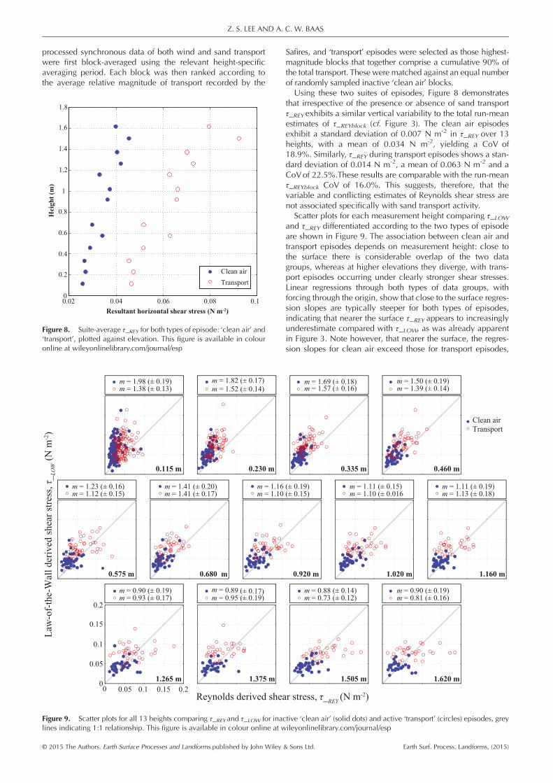
Figure 8. Suite-average τ_REY for both types of episode: ‘clean air’ and‘transport’, plotted against elevation. This figure is available in colouronline at wileyonlinelibrary.com/journal/esp

Figure 9. Scatter plots for all 13 heights comparing τ_REY and τ_LOW for inaclines indicating 1:1 relationship. This figure is available in colour online at w


Safires, and ‘transport’ episodes were selected as those highest-magnitude blocks that together comprise a cumulative 90% ofthe total transport. These were matched against an equal numberof randomly sampled inactive ‘clean air’ blocks.

Using these two suites of episodes, Figure 8 demonstratesthat irrespective of the presence or absence of sand transportτ_REY exhibits a similar vertical variability to the total run-meanestimates of τ_REYblock (cf. Figure 3). The clean air episodesexhibit a standard deviation of 0.007 N m-2 in τ_REY over 13heights, with a mean of 0.034 N m-2, yielding a CoV of18.9%. Similarly, τ_REY during transport episodes shows a stan-dard deviation of 0.014 N m-2, a mean of 0.063 N m-2 and aCoVof 22.5%.These results are comparable with the run-meanτ_REYblock CoV of 16.0%. This suggests, therefore, that thevariable and conflicting estimates of Reynolds shear stress arenot associated specifically with sand transport activity.

Scatter plots for each measurement height comparing τ_LOW

and τ_REY differentiated according to the two types of episodeare shown in Figure 9. The association between clean air andtransport episodes depends on measurement height: close tothe surface there is considerable overlap of the two datagroups, whereas at higher elevations they diverge, with trans-port episodes occurring under clearly stronger shear stresses.Linear regressions through both types of data groups, withforcing through the origin, show that close to the surface regres-sion slopes are typically steeper for both types of episodes,indicating that nearer the surface τ_REY appears to increasinglyunderestimate compared with τ_LOW, as was already apparentin Figure 3. Note however, that nearer the surface, the regres-sion slopes for clean air exceed those for transport episodes,

tive ‘clean air’ (solid dots) and active ‘transport’ (circles) episodes, greyileyonlinelibrary.com/journal/esp



particularly at the three lowest elevations. For both types ofepisodes, the slopes start to approach unity at elevations of0.46 m and above.With the exception of the lowest two measurement heights,

the similarity between regression slopes for both transport andclean air episodes, particularly in the context of their 95% con-fidence intervals, suggests that there is no sand transport impacton the relationship between τ_REY and τ_LOW, and a transport-dependent ‘apparent’ (or ‘variable’) von Kármán constant isnot suitable for relating the two. This contrasts with hydrody-namic studies which observe a stratified boundary layer in-duced by sediment loading, causing a divergence betweenat-a-point vertical turbulent momentum flux and τ determinedfrom a velocity profile (Smith and McLean, 1977; Adams andWeatherly, 1981; Kim et al., 2000). Li et al. (2010) postulatethat this effect is responsible for incompatible τ_LOW and τ_REYestimates at 1 m above the bed, during periods of active aeoliansand transport in their field experiments. Density stratificationand the associated ‘apparent’ von Kármán constant are unlikelyover the larger part of the vertical profile in our study, however,as our results show, only the lowest two measurement heightsdemonstrate any significant divergence in regression slopesbetween clean air and transport episodes. The observed dif-ferences between slope estimates at the lower elevations are,furthermore, the exact opposite to the postulated expectationsof sediment-laden boundary layer stratification, as our resultsnominally suggest that during active transport episodes thevon Kármán constant would require less adjustment to matchτ_LOW to τ_REY than under clean air conditions.

Evaluation

In boundary layer flows τ_REY and τ_LOW are typically assumedto be equivalent within the constant stress layer, but the obser-vations presented here indicate that they are fundamentallyconflicting on both a run-averaged and a time-series basis.Our results furthermore show that τ_REY varies irregularly acrossthe ’constant’ stress layer, with a 15–20% variability that greatlyexceeds individual confidence intervals.Data limitations or errors are unlikely sources for the discrep-

ancies observed here: quality was assured through a careful ex-perimental design and data selection, rigorous data cleaning,and robust pre-processing and analysis. Furthermore, spectralanalysis of the 50 Hz data at 0.115 m (i.e. the lowest elevation)indicates that the Kolmogorov micro-scale is reached before theNyquist frequency, suggesting minimal exclusion of high fre-quency turbulent energy from the data (van Boxel et al., 2004).It is acknowledged that sediment transport has the potential

to cause disagreement between shear stress estimates directly,by interrupting the sonic pathway, or impacting the ultrasonictransducers. While the discrepancy between τ_LOWblock andthe τ_REYblock at 0.115 m is significant (56.4% of the τ_LOWblock

magnitude), the difference is comparable with estimates de-rived at 0.68 m (56.9% of τ_LOWblock) or 1.16 m (59.2% ofτ_LOWblock). The discrepancies are, therefore, unlikely due tomechanical interference of saltating grains. More importantly,our results indicate that there is no justification for an ‘apparent’or variable von Kármán constant and we find that sedimenttransport is not likely responsible for the conflicting estimatesof τ_LOW and τ_REY.The discrepancies are not simply within normal error

bounds, and the τ estimates are based on robust statistics. Forexample, we record an R2 of 0.990 for the fit of the Law-of-the-Wall (through 13 points), an R2 comparable with many fieldand wind tunnel studies using far fewer measurement heights(Butterfield, 1999; Li, et al., 2010). Furthermore, our confidence


bounds are equal to 4.6% of the shear stress, smaller than thosereported by Namikas et al. (2003), for example, which rangefrom 7.1% to 12.0%.

In summary, the observed discrepancies, both between thetwo methods, as well as between heights in terms of Reynoldsderived stress, are significant and unlikely due to data or instru-ment error, nor due to sand transport effects. The discrepanciesnot only present significant problems for studying sedimenttransport dynamics in natural boundary layers, but our findingsalso challenge the notion that shear stress within the theoreticalframework of the Law-of-the-Wall is equivalent to the shearstress derived from the local Reynolds stress tensor, as well asthe presence of a ‘constant’ stress layer.

Our results show that a typical aeolian internal boundarylayer flow as is commonly measured in field studies may dis-play a near-perfect logarithmic velocity profile and yet at-a-point Reynolds shear stresses can vary considerably with heightand deviate significantly from the Law-of-the-Wall estimate.The internal variability in τ_REY of 19.8% for window-averagedestimates and 16.0% for block-averaged estimates is far in ex-cess of the definition of a constant stress layer, where variabilityin fluxes by elevation should remain below 10% of their mag-nitude (Stull, 1988).

The results demonstrate that τ_LOW is strictly a bulk propertyassociated with the entirety of the flow, while τ_REY corre-sponds to a single point within that flow, and critically thetwo are not equivalent on relevant time-scales. One potentialcause for the discrepancies, we hypothesise, is that the presenceof coherent flow structures in the turbulent flow (cf. Bauer et al.,2013) creates highly localised and persistent variability in thestress tensor at different points in the flow (hence affecting theReynolds shear stress), but they have less impact on the scalarwind speed used in the Law-of-the-Wall framework. Variabilityin streamwise vorticity, for example, will affect the stress tensorbut not the scalar wind speed. The potential influence of burst-ing events on flux profiles (Chen, 1990) may explain shear stressvariability on a time-series basis, on the temporal scale of theevents themselves, but would not explain the longer-termdiscrepancies and variability on the time-scale of the wholemeasurement run found in this study.

While we do not mean to challenge the validity of the con-stant stress layer concept (fundamentally a conservation of mo-mentum principle), our findings do question the typicalexpectation of the presence of a constant stress layer underthe kind of field conditions and site characteristics that wewould normally consider to be ideal and representative for (ae-olian) sediment transport studies (such as a long fetch distance,unidirectional winds, a flat and uniform sand surface, and avery high R2 goodness-of-fit for the Law-of-the-Wall). Conse-quently, it is difficult to differentiate between ‘simple’ boundarylayer conditions where Biron et al. (2004) recommend usingReynolds derived shear stress, or more complex flow condi-tions where Reynolds derived methods are found to be less re-liable (Kim et al., 2000). The use of streamline correctionroutines (van Boxel et al., 2004; Lee and Baas, 2012) and thecalculation of the resultant horizontal shear stress, however,should improve the use of Reynolds derived techniques irre-spective of the complexity of the surface topography.

Further research comparing the two methods with a simulta-neous direct measure of surface shear stress, using a drag platein a full-scale field experiment, may yield firmer guidance onmeasurement strategy and application. At present we recom-mend using τ_REY, albeit with careful consideration (streamlinecorrection, resultant horizontal). Our preliminary analysis ofcorrelations between τ_REY at different heights and sand trans-port suggests that for studies concerned with evaluating sedi-ment transport dynamics τ_REY should be measured as close



to the surface as possible, while avoiding any potential me-chanical interference of saltating grains.It may be fruitful to evaluate potential relationships between

turbulent kinetic energy (TKE) and sediment transport to facili-tate a move away from variable and conflicting estimates of τ.This suggestion is in agreement with recent studies of airflowover more complex surface topographies, for example: Smythet al. (2014) concerned with flow dynamics and associatedsediment transport patterns within a coastal trough blow out,and Chapman et al. (2013) who evaluated Reynolds stressand associated sediment transport over a coastal foredune.Methods to derive τ using a modified TKE are used in fluvialgeomorphology (Biron et al., 2004; Pope et al., 2006; Nosset al., 2010) based on a linear relationship between TKE andτ (Soulsby and Dyer, 1981; Kim et al., 2000). Research com-paring TKE with τ_LOW and τ_REY has typically found that theTKE method is more suitable in complex flow conditions(Biron et al., 2004; Bagherimiyab and Lemmin, 2013). Whileit is proposed that more specific investigation into TKE andsediment transport dynamics is required, the existing researchon TKE derived shear stress estimation is encouraging.

Acknowledgements—This research was carried out while Z. S. Lee wasin receipt of a UK Natural Environment Research Council DoctoralTraining Grant. The authors wish to thank Derek Jackson for the useof all the field equipment and to Thomas Smyth who secured accessto the field site and provided invaluable assistance in the field. Themanuscript was significantly improved and expanded based on theinsightful and constructive comments and suggestions from twoanonymous reviewers. We greatly thank them for encouraging us toconduct additional analysis and careful considerations of all aspectsof this study.

ReferencesAdams CE, Weatherly GL. 1981. Some effects of suspended sedimentstratification on an oceanic bottom boundary layer. Journal of Geo-physical Research, Oceans 86(C5): 4161–4172. DOI:10.1029/JC086iC05p04161.

Baas ACW. 2004. Evaluation of saltation flux impact responders (Safires)for measuring instantaneous aeolian sand transport intensity. Geomor-phology 59(1–4): 99–118. DOI:10.1016/j.geomorph.2003.09.009.

Baas ACW. 2008. Challenges in aeolian geomorphology: Investigatingaeolian streamers. Geomorphology 93(1–2): 3–16. DOI:10.1016/j.geomorph.2006.12.015.

Baas ACW, Sherman DJ. 2006. Spatio-temporal variability of aeoliansand transport in a coastal environment. Journal of Coastal Research22: 1198–1205. DOI:10.2112/06-0002.1.

Babaeyan-Koopaei K, Ervine DA, Carling PA, Cao Z. 2002. Velocity andturbulence measurements for two overbank flow events in RiverSevern. Journal of Hydraulic Engineering 128(10): 891–900.DOI:10.1061/(ASCE)0733-9429(2002)128:10(891).

Bagherimiyab F, Lemmin U. 2013. Shear velocity estimates in rough-bed open-channel flow. Earth Surface Process and Landforms 38:1714–1724. DOI:10.1002/esp.3421.

Bagnold RA. 1941. The Physics of Blown Sand and Desert Dunes.Chapman and Hall: London.

Barchyn TE, Martin RL, Kok JF, Hugenholtz CH. 2014. Fundamentalmismatches between measurements and models in aeolian sedimenttransport prediction: the role of small-scale variability. Aeolian Re-search 15: 245–251. DOI:10.1016/j.aeolia.2014.07.002.

Bauer BO, Walker IJ, Baas ACW, Jackson DWT, McKenna-Neuman C,Wiggs GFS, Hesp PA. 2013. Critical reflections on the coherentflow structures paradigm in aeolian geomorphology. Chapter 8 InCoherent Structures in Flows at the Earth’s Surface,Venditti JG, BestJL, Church M, Hardy RJ (eds). Wiley-Blackwell: Chichester, UK;111–134.

Biron PM, Lane SN, Roy AG, Bradbrook KF, Richards KS. 1998. Sensi-tivity of bed shear stress estimated from vertical velocity profiles: theproblem of sampling resolution. Earth Surface Processes and


Landforms 23(2): 133–139. DOI:10.1002/(SICI)1096-9837(199802)23:2<133::AID-ESP824>3.0.CO;2-N.

Biron PM, Robson C, Lapointe MF, Gaskin SJ. 2004. Comparing differ-ent methods of bed shear stress estimates in simple and complex flowfields. Earth Surface Processes and Landforms 29(11): 1403–1415.DOI:10.1002/esp.1111.

Butterfield GR. 1999. Application of thermal anemometry and high-frequency measurement of mass flux to aeolian sediment transportresearch. Geomorphology 29(1–2): 31–58. DOI:10.1016/S0169-555X(99)00005-7.

Chapman C, Walker IJ, Hesp PA, Bauer BO, Davidson-Arnott RGD,Ollerhead J. 2013. Reynolds stress and sand transport over aforedune. Earth Surface Processes and Landforms 38: 1735–1747.DOI:10.1002/esp.3428.

Chen F. 1990. Turbulent characteristics over a rough natural surfacepart II: responses of profiles to turbulence. Boundary-Layer Meteorol-ogy 52: 301–311. DOI:10.1007/BF00122092.

Delgado-Fernandez I, Jackson DWT, Cooper JAG, Baas ACW, BeyersJHM, Lynch K. 2013. Field characterization of three-dimensionallee-side airflow patterns under offshore winds at a beach-dune sys-tem. Journal of Geophysical Research, Earth Surface 118: 706–721.DOI:10.1002/jgrf.20036.

Dong Z, LuoW, Qian G, Lu P. 2008. Wind tunnel simulation of the three-dimensional airflow patterns around shrubs. Journal of Geophysical Re-search, Earth Surface 113: F02016. DOI:10.1029/2007JF000880.

Frisch U. 1995. Turbulence: the Legacy of AN Kolmogorov. CambridgeUniversity Press: Cambridge.

Garratt JR. 1990. The internal boundary layer – a review. Boundary-Layer Meteorology 50(1–4): 171–203. DOI:10.1007/BF00120524.

Heathershaw AD, Simpson JH. 1978. The sampling variability of theReynolds stress and its relation to boundary shear stress and drag co-efficient measurements. Estuarine and Coastal Marine Science 6(3):263–274. DOI:10.1016/0302-3524(78)90015-4.

Jackson DWT, Beyers M, Delgado-Fernandez I, Baas ACW, CooperJAG, Lynch K. 2013. Airflow reversal and alternating corkscrew vor-tices in foredune wake zones during perpendicular and oblique off-shore winds. Geomorphology 187: 86–93. DOI:10.1016/j.geomorph.2012.12.037.

Jegede OO, Foken T. 1999. A Study of the internal boundary layer dueto a roughness change in neutral conditions observed during theLINEX field campaigns. Theoretical and Applied Climatology 62(1–2): 31–41. DOI:10.1007/s007040050072.

Kaimal JC, Finnigan J. 1994. Atmospheric Boundary Layer Flows: TheirStructure and Measurement. Oxford University Press: New York.

Kim SC, Friedrichs CT, Maa JY, Wright LD. 2000. Estimating bottomstress in tidal boundary layer from acoustic Doppler velocimeterdata. Journal of Hydraulic Engineering 126(6): 399–406.DOI:10.1061/(ASCE)0733-9429(2000)126:6(399).

King J, Nickling WG, Gillies JA. 2008. Investigations of the law-of-the-wall over sparse roughness elements. Journal of Geophysical Re-search, [Earth Surface] 113: F02S07. DOI:10.1029/2007JF000804.

Lee ZS, Baas ACW. 2012. Streamline correction for the analysis ofboundary layer turbulence. Geomorphology 171–172: 69–82.DOI:10.1016/j.geomorph.2012.05.005.

Li B, Sherman DJ, Farrell EJ, Ellis JT. 2010. Variability of the apparentvon Kármán parameter during aeolian saltation. Geophysical Re-search Letters 37(15): L15404. DOI:10.1029/2010gl044068.

Lynch K, Delgado-Fernandez I, Jackson DWT, Cooper JAG, Baas ACW,Beyers JHM. 2013. Alongshore variation of aeolian sediment trans-port on a beach under offshore winds. Aeolian Research 8: 11–18.DOI:10.1016/j.aeolia.2012.10.004.

Martin RL, Barchyn TE, Hugenholtz CH, Jerolmack DJ. 2013. Timescaledependence of aeolian sand flux observations under atmospheric tur-bulence. Journal of Geophysical Research, [Atmospheres] 118:9078–9092. DOI:10.1002/jgrd.50687.

Namikas SL, Bauer BO, Sherman DJ. 2003. Influence of averaging inter-val on shear velocity estimates for aeolian transport modeling. Geo-morphology 53(3–4): 235–246. DOI:10.1029/JC082i012p01735.

Noss C, Salzmann T, Storchenegger I. 2010. Turbulent and advectivemomentum fluxes in streams. Water Resources Research 46:W12518. DOI: 10.1029/2010WR009297

Pope ND, Widdows J, Brinsley MD. 2006. Estimation of bed shearstress using the turbulent kinetic energy approach – a comparison



of annular flume and field data. Continental Shelf Research 26(8):959–970. DOI:10.1016/j.csr.2006.02.010.

Rao KS, Wyngaard JC, Coté OR. 1974. The structure of a two-dimensional internal boundary layer over a sudden change of surfaceroughness. Journal of the Atmospheric Sciences 31: 738–746.DOI:10.1175/1520-0469(1974)031<0738:TSOTTD>2.0.CO;2.

Shields A. 1936. Anwendung der Aehnlichkeitsmechanik und derTurbulenzforschung auf die Geschiebebewegung [Application ofsimilarity mechanics and turbulence research on shear flow].Mitteilungen der Preußischen Versuchsanstalt für Wasserbau (inGerman) 26. Berlin: Preußische Versuchsanstalt für Wasserbau.

Soulsby RL, Dyer KR. 1981. The form of the near-bed velocity profile ina tidally accelerating flow. Journal of Geophysical Research 86(C9):8067–8074. DOI:10.1029/JC086iC09p08067.

Smith JD, McLean SR. 1977. Spatially averaged flow over a wavy sur-face. Journal of Geophysical Research 82(12): 1735–1746. DOI:10.1029/JC082i012p01735.

Smyth TAG, Jackson D, Cooper A. 2014. Airflow and aeolian sedi-ment transport patterns within a coastal trough blowout during lateral


wind conditions. Earth Surface Processes and Landforms 39(14):1847–1854. DOI:10.1002/esp.3572.

Stull RB. 1988. An Introduction to Boundary Layer Meteorology.Springer.

Tennekes H, Lumley JL. 1972. A First Course in Turbulence. MIT Press:Cambridge, MA.

van Boxel JH, Sterk G, Arens SM. 2004. Sonic anemometers in aeoliansediment transport research. Geomorphology 59: 131–147.DOI:10.1016/j.geomorph.2003.09.011.

Voulgaris G, Trowbridge JH. 1998. Evaluation of the acoustic Dopplervelocimeter (ADV) for turbulence measurements. Journal of Atmo-spheric and Oceanic Technology 15(1): 272–289. DOI:10.1175/1520-0426(1998).

Walker IJ. 2005. Physical and logistical considerations of using ultra-sonic anemometers in aeolian sediment transport research. Geomor-phology 68: 57–76. DOI:10.1016/j.geomorph.2004.09.031.

Wilkinson RH. 1984. A method for evaluating statistical errors associ-ated with logarithmic velocity profiles. Geo-Marine Letters 3(1):49–52. DOI:10.1007/BF02463442.


king s research portal · the reynolds decomposition technique determines at-a-point shear stresses...

Documents