KINETIC THEORY AND MICRO/NANOFLUDICS

Kinetic Description of Dilute Gases

Transport Equations and Properties of Ideal Gases

The Boltzmann Transport Equation

Micro/Nanofludics and Heat Transfer

Kinetic Description of Dilute Gases

Hypotheses and Assumptions molecular hypothesis

▪ matter: composition of small discrete particles ▪ a large number of particles in any macroscopic volume (27×106 molecules in 1-m3 at 25ºC and 1 atm)

statistic hypothesis

▪ long time laps: longer than mean-free time or relaxation time ▪ time average

simple kinetic theory of ideal molecular gases limited to local equilibrium based on the mean-free-path approximation

kinetic hypothesis

▪ laws of classical mechanics: Newton’s law of motion molecular chaos

▪ velocity and position of a particle: uncorrelated (phase space)

▪ velocity of any two particles: uncorrelated ideal gas assumptions

▪ molecules: widely separated rigid spheres

▪ elastic collision: energy and momentum conserved

▪ negligible intermolecular forces except during collisions

▪ duration of collision (collision time) << mean free time

▪ no collision with more than two particles

Distribution Function: particle number density in the phase space at any time

( , , )f r v t

6 ( , , ) x y zd N f r v t dxdydzdv dv dv 3 3( , , )f r v t d Vd

3 3, x y zd V dxdydz d dv dv dv

▪ number of particles per unit volume (integration over the velocity space)

63

3 ( , , )d N

f r v t dd V

33

3 ( , , )d N dN

f r v t dd V dV

( , )n r t

▪ number of particles in a volume element of the phase space in

,r dr v dv

▪ total number of particles in the volume V

( , ) ( , )r t m n r t

density:

3 3( ) ( , , )V

N t f r v t d Vd

In a thermodynamic equilibrium state, the distribution function does not vary with time and space.

( , , ) ( )f r v t f v

3( , , )dN

f r v t ddV

Local Average and Flux

( , , )r v t

: additive property of a single molecule such as kinetic energy and momentum▪ local average or simply average

(average over the velocity space)

( , )f d

r tfd

1

( , )f d

n r t

▪ ensemble average (average over the phase space)

V

V

f dVd

fdVd

1

( ) Vf dVd

N t

▪ flux of : transfer of across an area element dA per unit time dt per unit area

number of particles with velocities between and that passes through the area dA in the time interval dt

v

v dv

cosdV vdt dA

dA

vdt

v n̂

ˆv ndAdt

dt is so small that particle collisions can be neglected.

ˆ( , , ) ( , , )f r v t dVd f r v t v ndAdtd

ˆ( , , )f r v t v ndAdtd

dAdt

total flux of :

ˆJ fv nd

flux of within d

▪ particle flux:

1

ˆNJ fv nd

In an equilibrium state ( , , ) ( )f r v t f v

2 sind v d d dv ˆ( )NJ f v v nd

2 / 2 2

0 0 0( ) cos sin

vf v v v d d dv

2 / 2 3

0 0 0( ) cos sin

vf v v d d dv

3

0( )

vf v v dv

NJ

For an ideal gas: Maxwell’s velocity distribution 3/ 2 2

B B

( ) exp2 2

m mvf v n

k T k T

▪ average speed1

( , )r t f dn

2 3

0 0 0

1 1( ) sin

vv fvd f v v d d dv

n n

3

0

4( )

vf v v dv

n

3

0( )N

vJ f v v dv

4

nv

For an ideal gas: Maxwell’s velocity distribution

B8,

k Tv

m B

2N

k TJ n

m

▪ mass flux

ˆ( )4

m

vJ m f v v nd

ˆ , NJ fv nd nm

▪ kinetic energy flux

2

2

mv

25

KE0

ˆ ( )2 2

mv mJ fv nd f v v dv

KEJ

▪ momentum flux

, , 1, 2,3ij j iP mv fv d i j

1

( , )r t f dn

ij i jP m fv v d

1

i j i jmn fv v d mnv vn

i j ij ijv v P

11

The Mean Free Path

Mean Free Path :average distance between two subsequent collisions for a gas molecule.

dd 2d

m0 m1 m1 m2

Mean Free Path

12

number of collisions per unit time : (frequency)

ndV particles will collide with the moving particle.

dd 2d

vdt

2dV d vdt

2nd v

2

1v

nd

1

frequency

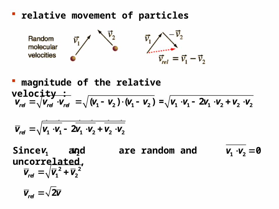
relative movement of particles

magnitude of the relative velocity :

rel rel relv v v

1 2 1 2( ) ( )v v v v

1 1 1 2 2 2= 2v v v v v v

1 1 1 2 2 22relv v v v v v v

1 2 0v v

Since and are random and uncorrelated,1v

2v

2 21 2relv v v

2relv v

14

relative movement of particles

: based on the Maxwell velocity distribution

- Ideal gas

relative 2 2 2

1 1 1

( 2 ) 2rel

v v vnd v nd v nd

PV nRT , AB A

N nR k N n

V B Ank N T

BP nk T

relative2

1

2B

Pd

k T

22Bk T

d P

15

: probability that a molecule travels at least between collisions

Probability for the particle to collide within an element

distance d:

probability to travel at least + d between collision

probability not to collide within + d

probability not to collide within d

( )p

d

( ) ( ) 1d

p d p

16

Probability density function (PDF) :

( ) ( ) 1d

p d p

( )( ) ( ) ( )

dp dp d p p

d

( ),

( )

dp d

p

( )

(0) 0

1 1p

pdp d

p

( )

(0)0

ln ( ) ,p

pp

ln ( ) ln (0)p p

/( )p e

/( ) 1( )

dpF e

d

(0) 1p

17

( )F is the mean free-path PDF.

0( ) 1F d

0( )F d

/

0

1 e d

/ /

00

1e e d

// 0

1lim e

e

2/ /

1 1lim lim 1

e e

18

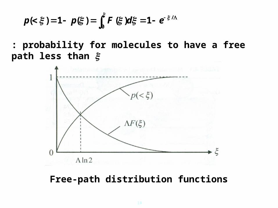
: probability for molecules to have a free path less than

Free-path distribution functions

/

0 ( ) 1 ( ) ( ) 1p p F d e

Molecular gas at steady state

(Local equilibrium)

Average collision distance

Average Collision Distance

a a

0

Transport Eqs and Properties of Ideal Gases

(r, v, ) ( , v)f t f

2 / 2

0 02 / 2

0 0

cos cos

cos sina

dA d d

dA d d

2 233

dA

dA

21/( 2 )d n dAcos: projected area: coordinate along gradientcos: average projected length

Shear Force and Viscosity

Momentum exchange between upper layer and lower

layerAverage momentum of particles

Momentum flux across y0 plane

)(B y

Velo

cit

y in

y d

irecti

on

Flow direction, x

a0 y

a0 y

0yB0

area)unit per frequency (Collisionflux Molecular :4/n

speedmolecular Mean :/8ity,Bulk veloc :)(B mTky B

a

a

( ) ( )x Bp y m y

0

04B

P B a

y

dnJ m

dy

0

04B

P B a

y

dnJ m

dy

Net momentum flux : Shear force

Dynamic viscosity : Order-of-magnitude estimate

Dynamic viscosity from more detailed calculation and experiments

Simple ideal gas model → Rigid-elastic-sphere model

0 0

1

3B B

p p p yx

y y

d dJ J J

dy dy

2

/1 2

3 3Bmk T

d

1, , ( )P f T

weak dependence on pressure

22

1 1

2 2 2Bmk Tm

dd

Heat Diffusion

Molecular random motion →

Thermal energy

transfer

Net energy flux across x0 plane

Tem

pera

ture

, T

x direction

0xa0 x a0 x

0T

)( moleculeper energy thermalAverage : Tf

aa

E E E xJ J J q

0 0( ) ( )4 a a

nx x

0

1

3 x

dn

dx

Heat flux

T dependence

Thermal conductivity

0

1

3E E E xx

dJ J J q n

dx

0

1

3 vx

dTc

dx

0 0 0

vx x x

d d dT dTn n nmc

dx dT dx dx

2

1 2

3 3v

mkTc c

d

1 , & ( ) vc f T

Monatomic gas

Diatomic gas

< Tabulated values for real gases

≈ Tabulated values for real gases

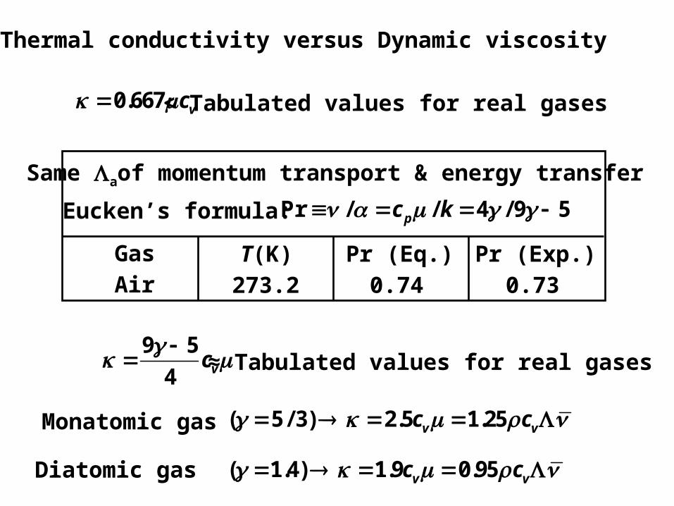
Thermal conductivity versus Dynamic viscosity

Gas T(K) Pr (Eq.) Pr (Exp.)Air 273.2 0.74 0.73

Eucken’s formula:

0.667 vc

Pr / / 4 / 9 5pc k

Same aof momentum transport & energy transfer

9 5

4 vc

( 5 / 3) 2.5 1.25v vc c

( 1.4) 1.9 0.95v vc c

Mass Diffusion

Fick’s lawGas AnA = nnB = 0

Gas BnA = 0nB = n

x direction

nA(x) nB(x)

B andA between t coefficienDiffusion :ABD

rate transfer Mass : rate,transfer Molecular : AJmAJNAA mANA

AN

BN A

AN AB

dnJ D

dx

A

Am AB

dJ D

dx

B

BN BA

dnJ D

dx

B

Bm BA

dJ D

dx

distance, Central :2/)( BA ddd mass Reduced :)/( BABAr mmmmm

Diffusion coefficient

Net molecular flux

Uniform PA BN NJ J

0 0

A AA 0 a A 0 a( ) ( )

4 4ANx x

dn dnJ n x n x

dx dx

0

A1

3 x

dn

dx

AB 2r

1 3 1

3 8 2Bk T

Dnd m

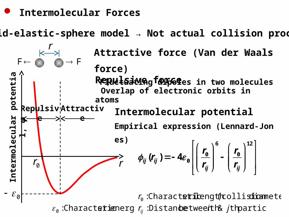
Intermolecular Forces

Rigid-elastic-sphere model → Not actual collision process

Attractive force (Van der Waals force) Fluctuating dipoles in two molecules

Repulsive force Overlap of electronic orbits in atoms

Intermolecular potentialEmpirical expression (Lennard-Jones)

r

0

0r

Attractive

Repulsive

F F

Inte

rmol

ecul

ar p

oten

tial,

φ

r

diameter) (collisionlength sticCharacteri :0r

particlesth &th between Distance : jirijenergy, sticCharacteri :0

6 12

0 00( ) 4ij ij

ij ij

r rr

r r

Computer simulation of the trajectory of each moleculeMolecular dynamic is a powerful tool for dense phases, phase change

→ Not good for dilute gas → Direct Simulation Monte Carlo (DSMC)

Force between molecules

Newton’s law of motion for each molecule

13 7

0 0 0

0

r242 ij

ij ijij ij ij

r rF

r r r r

vF (r ,r , ) , 1,2, ...,i

ij i j ij

dt m i N

dt

: mean free path [m]u : energy density of particles [J/m3] : characteristic velocity of particles [m/s]

Taylor series expansion

heat flux in the z-direction

Thermal Conductivity

z +z

z

z - z

( )zu z

zq

cos ,z coszv v

1( ) ( )

2z z z zq v u z u z

and( ) ( )z z

duu z u z

dz ( ) ( )z z

duu z u z

dz

v

Averaging over the whole hemisphere of solid angle 2

1( ) ( )

2z z z z

du duq v u z u z

dz dz

2cosz z

du duv v

dz dz

2 / 2 2

0 0

1cos sin

2z

duq v d d

dz

zq

1

3

duv

dz

cos , cosz zv v

Assuming local thermodynamic equilibrium: u is a function of temperature

Fourier law of heat conduction

First term : lattice contribution

Second term : electron contribution

1 1 1

3 3 3z

du du dT dTq v v Cv

dz dT dz dz

z

dTq k

dz

1

3k C v

1

3l ek C v C v

v

r

F

r dr

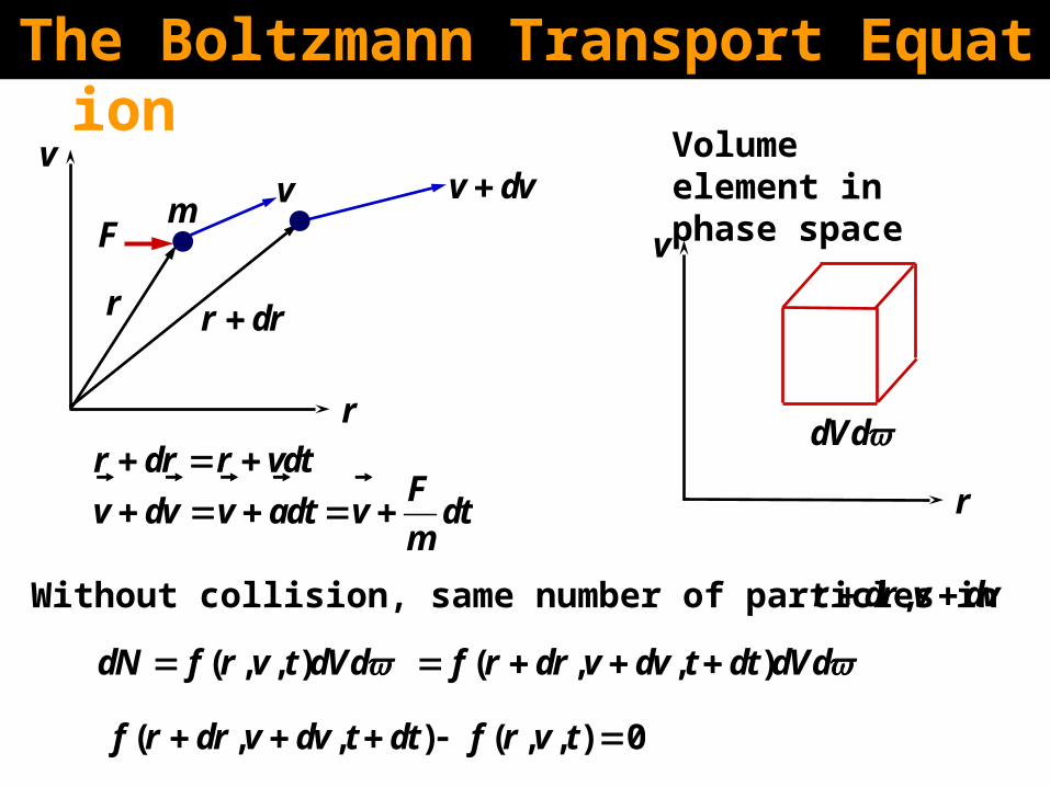
v dv Volume

element in phase spacev

r

dVdr dr r vdt

Fv dv v adt v dt

m

Without collision, same number of particles in ,r dr v dv

( , , )dN f r v t dVd

( , , )f r dr v dv t dt dVd

( , , ) ( , , ) 0f r dr v dv t dt f r v t

v

m

r

The Boltzmann Transport Equation

( , , ) ( , , )f f f

f r dr v dv t dt f r v t dt dr dvt r v

( , , ) ( , , )f r dr v dv t dt f r v t f f dr f dv

dt t r dt v dt

0f f f

v at r v

ˆ ˆ ˆr

f f f ff i j k

r x y z

ˆ ˆ ˆvx y z

f f f ff x y z

v v v v

Liouville equationIn the absence of collision and body force

0Df f f

vDt t r

With collisions, Boltzmann transport equation

coll

f f f fv a

t r v t

coll

f

t

: number of particles that join the group in as a result of collisions

,r dr v dv

: number of particles lost to the group as a result of collisions

coll

( , ) ( , , ) ( , ) ( , , )v

fW v v f r v t W v v f r v t

t

( , )W v v: scattering probability the fraction of particles with a velocity that will change their velocity to per unit time due to collision

v

v

Relaxation time approximation

under conditions not too far from the equilibrium

0

coll ( )

f f f

t v

f0 : equilibrium distribution: relaxation time

Hydrodynamic EquationsThe continuity, momentum and energy equations can be derived from the BTE

The first termlocal average

( )f f f

d v d a d dt r v

1f d

n

( )f nd fd f d n

t t t t t

The second term

vf vf vf

fv v f

r

vf f v v f

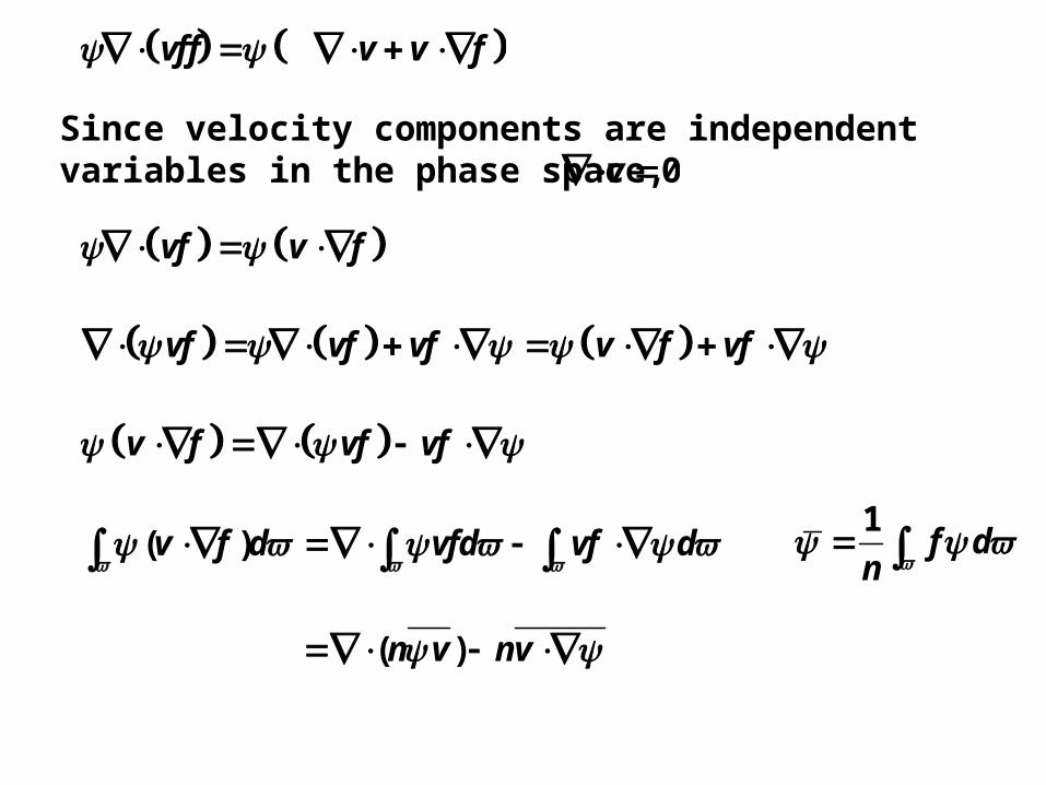
Since velocity components are independent variables in the phase space, 0v

vf v f

( )n v nv

1f d

n

vf vf vf v f vf

v f vf vf

( )v f d vfd vf d

The third term

, ,

, ,

x x x

x x x

v v v

v v v

fa d a f f d na

v v v

( )F ra

m

Integrating by parts

( )( )

nn n v nv na

t t v

( ) ( )n n v n v at t v

( )d

m When

( ) ( ) 0m m

nm nmv n v m at t v

nm

B B( ) 0 0D

v vt Dt

or

Continuity equation

B R=v v v

Bv

Rv

: bulk velocity,

: random velocity

B R B R B=v v v v v v

( ) ( )n n v n v at t v

Momentum equation

When mv

: shear stress

( ) ( )n n v n v at t v

B R B R B B R R B R= 2vv v v v v v v v v v v

B B R R B R B B R R2v v v v v v v v v v

R Rv v

( ) ( ) 0mv mv

nmv nmvv n v mv at t v

BB B( ) ( )

vnmv v v

t t t t

B B R R B B R R( )nmvv v v v v v v v v

BB B B B B( ) ( ) = 0ij

vv v v v v P a

t t

B B B B ijv v v v P

0,mv

nt

0,nv mv

( ) ( ) 0mv mv

nmv nmvv n v mv at t v

mvna a

v

combination of all terms

applying the mass balance equation

BB B B B B( ) ( ) = 0ij

vv v v v v P a

t t

BB B B B( ) ( ) = 0ij

vv v v v P a

t t

B 1ij

DvP a

Dt

B

22 ,

3

,

i

i

ijji

j i

vP v i j

xP

vvi j

x x

Energy equation

: only random motion contributes to the internal energy

( ) ( )n n v n v at t v

2R

1

2mv

2 2B R R R B E

1 1( )

2 2n v v v v v uv J

u: mass specific internal energy

: energy flux vectorE RJ n fv d

2R

1( )

2n n mv u

t t t

( ) ( )n n v n v at t v

2R

12

0mv

n nt t

2R R B

1( - )

2nv nv mv v v v v

R B B( ) :ijv v v P v i

iji j j

vP

v

2R

R

12

0mv

na na a vv v

B E B( ) ( ) : 0iju uv J P vt

using the continuity equation

E B:ij

DuJ P v

Dt

Fourier’s Law and Thermal conductivity

BTE under RTA

Assume that the temperature gradient is in the only x-direction, medium is stationary local average velocity is zero, distribution function with x only at a steady state

If not very far away from equilibrium

0

( )

f ff f fv a

t r v v

0x

f ffv

x

0ff

x x

0

0 ,x

fv f f

x

0

0 ,x

ff f v

x

0

0 x

f dTf f v

T dx

0

( )

f ff fv

t r v

heat flux in the x direction

Under local-equilibrium assumption and applying the RTA

0E, 0x x x x x

f dTJ q f v d f v v d

T dx

0 0,xf v d

1

3xv v

x

dTq k

dx : 1-D Fourier’s

law

201

3

fk v d

T

: 3-D Fourier’s law

Eq J fv d k T

00 x

f dTf f v

T dx

Microdevices involving fluid flow : microsensors, actuators, valves, heat pipes and microducts used in heat engines and heat exchangers

Biomedical diagnosis (Lab-on-a-chip), drug delivery, MEMS/NEMS sensors, actuators, micropump for ink-jetprinting, microchannel heat sinks for electronic coolingFluid flow inside nanostructures, such as nanotubes and nanojet

Micro/Nanofluidics and Heat Transfer

The Knudsen Number and Flow Regimes

ratio of the mean free path to the characteristic length

Knudsen Number

Knudsen number relation with Mach number and Reynolds number

KnL

Re ,L

L

a

Ma

,a RT 2 /RT

: ratio of specific heat

Re = 2 / Re 2 /

L

L

L L

RT RT

Ma Ma RTRT

= = 2 ReRe 2 / Re 2 / LL L

Ma RT MaKn

RT RT

Knudsen Number

Rarefaction or Continuum

Regime Method of calculation Kn range

Continuum

Navier-stokes and energy equation with no-slip /no-jump boundary conditions

Slip flow Navier-stokes and energy equation with slip /jump boundary conditions/DSMC

Transition BTE, DSMC

Free molecule

BTE, DSMC

Flow Regimes based on the Knudsen Number

0.001Kn

0.001 0.01Kn

0.1 10Kn

10Kn

Flow regimes

1. Continuum flow (Kn < 0.001)

The Navier-Stokes eqs. are applicable.The velocity of flow at the boundary is the same as that of the wall

The temperature of flow near the wall is the same as the surface temperature.

Conventionally, the flow can be assumed compressibility. If Ma < 0.3, the flow can be assumed incompressible.Consider compressibility : pressure change, density change

centerline

13

2

Velocity profilesTemperature profiles

by

( )x y

xy 1

2

3

( )T y

wT

2. Slip flow (0.001 < Kn < 0.1)

Non-continuum boundary condition must be applied.

The velocity of fluid at the wall is not the same as that of the wall(velocity slip).

The temperature of fluid near the wall is not the same as that of the wall (temperature jump).

centerline

13

2

Velocity profilesTemperature profiles

by

( )x y

xy 1

2

3

( )T y

wT

3. Free molecule flow (Kn > 10)

The continuum assumption breaks down.

The “slip” velocity is the same as the velocity of the mainstream.

The temperature of fluid is all the same : no gradient exists

The BTE or the DSMC, are the best to solve problems in this regime.

centerline

13

2

Velocity profilesTemperature profiles

by

( )x y

xy 1

2

3

( )T y

wT

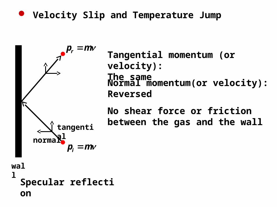
Velocity Slip and Temperature Jump

tangentialnorma

l

wall

Tangential momentum (or velocity):The sameNormal momentum(or velocity):Reversed

Specular reflection

No shear force or friction between the gas and the wall

rp m

ip m

Diffuse reflection

For diffuse reflection, the molecule is in mutual equilibrium with the wall.For a stream of molecule, the reflected molecules follow the Maxwell velocity distribution at the wall temperature.

Momentum accommodation coefficient

tangential components

normal components

w

(the incident)

(the reflected)

(the MVD corresponding to T )

i

r

w

For specular reflection

For diffuse reflection

i r

i w

p p

p p

i r

i w

p p

p p

p mv i: incident, r: reflectedw: MVD corresponding to Tw

0v v

1v v

Thermal accommodation coefficient

For specular reflection

For diffuse reflection

For monatomic molecules, T involves translational kinetic energy only which is proportional to the temperature (K).

i rT

i w

, i.e., 0i r T

, i.e., 1r w T

i rT

i w

T T

T T

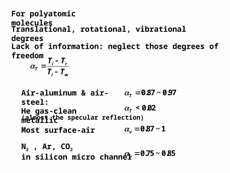
For polyatomic moleculesTranslational, rotational, vibrational degrees

Lack of information: neglect those degrees of freedom

Air-aluminum & air-steel:He gas-clean metallic(almost the specular reflection)

Most surface-air

N2 , Ar, CO2 in silicon micro channel

i rT

i w

T T

T T

0.87 ~ 0.97T

< 0.02T

0.87 ~ 1v

0.75 ~ 0.85v

Velocity slip boundary condition

Temperature jump boundary condition

2( ) 3

8bb

v xx b

yv y

v R Tv y

y T x

2 ( )2 2( )

1 Pr 4b

x bTb w

T y

v yTT y T

y R

Poiseuille flow

Assume that W >> 2H, edge effect can be neglected.incompressible and fully developed with constant properties

When Kn = /2H < 0.1

wq

x

2HW

x

y

Navier-Stokes equations

2Dup u f

Dt

fully developed flow2

2

1xv dp

y dx

/y H Let

2

2

1

( )xv dp

H dx

2 2

2xv H dp

dx

or

Velocity slip boundary condition

2( ) 3

8bb

v xx b

yv y

v R Tv y

y T x

neglecting thermal creep

The symmetry condition

2( )

b

v xx b

v y

dvv y

dy

2( ) = v x

xv

dvv

H d

1

2( 1) v x

xv

dvv

H d

2 v

vv

Kn

Let

1

( 1) 2 xx v

dvv

d

0

0xdv

d

2 2

2xv H dp

dx

2

1xv H dp

Cdx

0

0xdv

d

1 0C

22

2

1( )

2x

H dpv C

dx

1

( 1) 2 xx v

dvv

d

2

2(1)2x

H dpv C

dx

2

2

1

2 xv

dv H dpC

d dx

2 2

2 22v

H dp H dpC

dx dx

2 12

2v

dp H

dx

bulk velocity

2 221 1

( ) 22 2x v

H dp dp Hv

dx dx

2

2( ) 4 12x v

dp Hv

dx

1 1 2

2

0 0

( ) 4 12m x v

H dpv v d d

dx

1

3

0

2 14

2 3v

H dp

dx

2

1 63v

H dp

dx

velocity distribution in dimensionless form

Define the velocity slip ratio

: the ratio of the velocity of the fluid at the wall to the bulk velocity

velocity distribution in terms of slip ratio

22

2

4 12( )

1 63

vx

mv

dp Hdxv

v H dpdx

23 1 4( )

2 1 6vx

m v

v

v

( 1)x

m

v

v

3 1 4 1 6

2 1 6 1 6v v

v v

2( ) 3 3(1 )

2 2x

m

v

v

Energy equation

2p

DTc k T p v

Dt

2

2p x

T Tc v

x y

thermally fully developed condition with constant wall heat flux

2

2x

m

v

v

2 ( )2 2( )

1 Pr 4b

x bTb w

T y

v yTT y T

y R

temperature jump boundary condition

2 2( )

1 Prb

Tb

T y

yy

2 2 2( )

1 2 PrT

T H

2 2( ) 2

1 PrT

T

Kn

2 2

1 PrT

TT

Kn

Let

( ) 2 T

0

0d

d

The symmetry condition

22

2

3 3(1 )

2 2x

m

v

v

31

3 (1 )

2 2C

0

0d

d

1 0C

2 41 2

3 (1 )( )

4 8C C

1

( 1) 2 T

2 2

3 (1 ) 5( 1)

4 8 8C C

1

3 (1 )2 2 2

2 2T T T

2

52

8 TC

2 43 (1 ) 5( ) 2

4 8 8 T

dimensionless temperature

By boundary condition

: temperature-jump distance

bulk temperature

( ) w

w

T T

H q

( 1)w

w

T Tq

H

( 1) 2 T

2 2w w

wT T

T T T Tq

H H

2 T H

1

0

( )( )x

m mm

vd

v

2

2x

m

v

v

1 2

20

( )m m d

integration by parts 1 2

20

( )m d

1

0

1( )

0d

m

33 (1 ),

2 2

2 43 (1 ) 5

( ) 24 8 8 T

1

2 4 3

0

3 (1 ) 5 3 (1 )2 2

4 8 8 2 2T T

213

0

3 (1 )

2 2d

1 2 2 22 6 4

0

9 6 1 2 3 4

4 4 2d

2204 72 8

420

251 18 22

105m T

Nusselt number

hLNu

" 4 4h w

w m m

hD q HNu

T T

( )w w mq h T T 4 hD H( )m w

mw

T Tk

H q

2 2

4 140

68 24 (8 / 3) 280 17 6 (2 / 3) 70

140T T

Nu

Poiseuille flow

Poiseuille flow with one of the plate being insulated

circular tube of inner diameter D

2

140

17 6 (2 / 3) 70 T

Nu

2

140

26 3 (1/ 3) 70 T

Nu

2

48

11 6 48w

Dw m T

q DNu

T T k

Gas Conduction-from the Continuum to the Free Molecule RegimeHeat conduction between two parallel surfaces filled with ideal gases

1 2DF

T Tq

L

1T 2T

Lx

diffusion

jumpFree molecule

1T 2T

Lx

( )dT

q Tdx

9 5

4 vc

When Kn = /L << 1, diffusion regime

23/ 2 3 / 21 2

m,DF1 2

2

3

T TT

T T

2/ 3

3 / 2 3 / 2 3 / 21 1 2( )

xT x T T T

L

effective mean temperature and distribution

When Kn = /L >> 1, free molecule regime

Assume that T are the same at both walls.

1 21

(1 ),

2T

T

T TT

2 1

2

(1 )

2T

T

T TT

effective mean temperature

1 2m,FM 2

1 2

4T TT

T T

2 1FM

m,FM2 8

1T

T v

T Tq

RT

c P

net heat flux

For intermediate values of Kn,

2 1

,FM

,DF

2 9 51

1mT

T m

T Tq k

TL Kn

T