kinetic modeling of phase transformations occurring in the ... · of gas tungsten arc (gta) welds...

Acta Materialia 51 (2003) 3333–3349www.actamat-journals.com

Kinetic modeling of phase transformations occurring in theHAZ of C-Mn steel welds based on direct observations

J.W. Elmera,∗, T.A. Palmera, W. Zhangb, B. Wooda, T. DebRoyb

a Lawrence Livermore National Laboratory, University of California, P.O. Box 808, Livermore, CA 94551, USAb The Pennsylvania State University, University Park, PA 16802, USA

Received 18 November 2002; accepted 13 January 2003

Abstract

In situ Spatially Resolved X-Ray Diffraction (SRXRD) experiments were performed in the heat-affected zone (HAZ)of gas tungsten arc (GTA) welds of AISI 1005 C-Mn steel to directly observe welding induced phase transformations.These real-time observations were semi-quantified using diffraction peak profile analysis to construct a phase transform-ation map revealing ferrite (a) and austenite (g) phase concentration gradients in the HAZ. Weld thermal cycles werecalculated using a three-dimensional heat transfer and fluid flow model and then combined with the SRXRD phasemap to provide a complete description of the HAZ under actual welding conditions. Kinetic modelling of thea→gphase transformation during heating was performed using a Johnson–Mehl–Avrami analysis, modified to take intoaccount non-uniform weld heating and transformation in theα+γ two-phase field. The results provide the most accurateJMA kinetic parameters to date for this alloy, n=1.45 and 1n(ko)=12.2, for an activation energy Q=117.1 kJ/mole.Using this kinetic description of thea→g phase transformation, time temperature transformation (TTT) and continuousheating transformation (CHT) diagrams for this alloy were constructed to illustrate how the combination of SRXRDexperiments and numerical modeling from one weld can be used to predict phase transformations for a variety ofwelding and heat treating applications. 2003 Acta Materialia Inc. Published by Elsevier Science Ltd. All rights reserved.

Keywords: Spatially resolved X-ray diffraction; Phase transformations; Kinetics; Welding; Steels

1. Introduction

The investigation of phase transformations insteels is important because of the extensive rangeof microstructures and the resulting mechanicalproperties that steels can achieve through different

∗ Corresponding author. Tel.:+1-925-422-6543; fax:+1-925-423-7040.

E-mail address: [email protected] (J.W. Elmer).

1359-6454/03/$30.00 2003 Acta Materialia Inc. Published by Elsevier Science Ltd. All rights reserved.doi:10.1016/S1359-6454(03)00049-1

processing conditions. Transformations betweenthe body centered cubic (bcc) form of iron (a-ferrite) and the face centered cubic (fcc) form ofiron (g-austenite) are principally responsible for themicrostructure and properties of steels, and thetransformation between the two phases has beenstudied in great detail for many decades[1–3].Optimized thermal–mechanical processing treat-ments for wide varieties of steels have been estab-lished[4–6]. However, when steels are welded, theoptimized base metal properties are altered by the

3334 J.W. Elmer et al. / Acta Materialia 51 (2003) 3333–3349

localized weld thermal cycles. The result is the cre-ation of microstructures in the fusion zone (FZ)and heat affected zone of the welds that are sig-nificantly different than those of the base metal,creating non-optimal properties in welded joints[7–10].

In a previous paper SRXRD was used to investi-gate microstructural evolution in the HAZ of AISI1005 steel welds by directly identifying and map-ping the phases that exist in the HAZ during weld-ing [11]. For this C-Mn steel, regions of annealing,recrystallization, partial transformation and com-plete transformation to a-Fe, g-Fe, and d-Fe phaseswere identified using SRXRD in a qualitativefashion, however, the results were not quantifiedat that time. Further analysis of the major Braggreflections in the SRXRD patterns showed that sig-nificant additional information was contained inthe data regarding the relative fractions of the aand g phases present during the transformation.Some of this data was used to provide a semi-quan-titative measure of the relative fractions of a andg present during the a→g transformation on heat-ing. From this semi-quantitative SRXRD data, kin-etic information about the a→g phase transform-ation on heating was extracted [12,13] using amodified non-isothermal Johnson–Mehl–Avrami(JMA) analysis and the results of a well testedthree-dimensional (3D) numerical heat transfer andfluid flow model [14–17].

In this paper, previously published SRXRDresults [11] are analyzed to produce the entiresemi-quantitative phase map of the a→g→a phasetransformation in the HAZ of AISI 1005 steel. Thismap represents a considerable amount of effort andreveals for the first time this important phase trans-formation sequence in steel under the thermalcycles produced during arc welding. Analysis ofthis data using transport phenomena based numeri-cal modeling determined the kinetics of the phasetransformations under various thermal cycles,which can be used to predict a→g phase transform-ations under a wider range of welding conditionsthan can be studied by SRXRD alone.

2. Experimental procedures

2.1. SRXRD experiments

Gas tungsten arc (GTA) welds have been madeon AISI 1005 steel (0.05 C, 0.31 Mn, 0.18 Si, 0.11Ni, 0.10 Cr, 0.009 P, 0.008 Cu, 0.005 S, �0.005Al, �0.005 Nb, �0.005 Mo, �0.005 Ti, �0.005V; by wt. percent) cylindrical forged bar samples.These samples were machined from 10.8 cm diam-eter forged bar stock into welding samples, 12.7cm long and 10.2 cm diameter. Circumferentialwelds were then made on the cylindrical steel barsin an environmentally sealed chamber to avoidatmospheric contamination of the weld. A briefsummary of the welding parameters used here isgiven in Table 1. Further details of the weldingexperiments have been previously reported [11].

The in situ SRXRD experiments reported herewere performed during welding using the 31-polewiggler beam line, BL 10-2 [18] at SSRL withSPEAR (Stanford Positron-Electron AccumulationRing) operating at an electron energy of 3.0 GeVand an injection current of ~100 mA. In theseexperiments a focused monochromatic synchrotronX-ray beam is passed through a 260 µm tungstenpinhole to render a sub-millimeter beam on thesample at an incident angle of ~25°. This setupyields a beam flux on the sample of ~1010

photons/s, which was determined experimentallyusing an ion chamber immediately downstreamfrom the pinhole. A photon energy of 12.0 keV(l = 0.1033 nm) was chosen to facilitate phase

Table 1Summary of GTA welding parameters used in the SRXRDexperiments

Welding electrode W-2% ThElectrode diameter (mm) 4.7Torch polarity DCENMaximum current (A) 130Background current (A) 90Weld voltage (V) 17.5Pulsing frequency (Hz) 300Peak on time (%) 50Shielding gas HeliumTravel speed (mm/sec) 0.6Resulting fusion zone width (mm) ~9

3335J.W. Elmer et al. / Acta Materialia 51 (2003) 3333–3349

identification and to be far enough in energy abovethe Fe K-edge (7.112 keV) to minimize the back-ground contribution due to Fe K-fluorescence fromthe steel sample [23].

X-ray diffraction patterns at each location wererecorded using a 50 mm long 2048 element pos-ition sensitive Si photodiode array detector. Thearray was mounted on a dual-stage water cooledPeltier effect thermoelectric cooler at a distance ofapproximately 10 cm behind the weld to cover a2q range from 25–55°. This 2q range was optim-ized to contain a total of six diffraction peaks, threefrom the bcc phases (a-Fe or d-Fe) and three fromthe fcc phase (g-Fe). During a typical SRXRD run,40 diffraction patterns were gathered at intervalsof 250 µm along a pre-determined path, spanninga range of 10 mm through the HAZ. The accuracyof the positioning of the SRXRD beam withrespect to the fusion boundary for a given weld is±0.5 mm. This estimate considers the initial pos-itioning the X-ray beam, and dynamic fluctuationsin the fusion boundary as discussed elsewhere forthese 1005 steel welds [11]. Additional details ofthe SRXRD experiments are published elsewhere[19–22].

2.2. Diffraction pattern profile analysis

Analysis of each peak in each diffraction patternwas performed to determine the semi-quantitativevolume fractions of ferrite and austenite present ateach SRXRD location. This analysis measured theintegrated intensity of each peak in each diffractionpattern using a sum of one or more Gaussian peakprofile fitting functions [21,24]. The area andFWHM values of the fitted peaks were thendetermined using an automated curve-fitting rou-tine developed in Igor Pro , Version 4.0 [25].

The raw integrated intensities of the diffractionpeaks were then converted into relative phaseintensities. This conversion is based on the effectsof a number of factors on the resulting intensityof a given peak. In this method, the peak area orintegrated intensity of each peak is measured andthen converted to relative fraction of each phaseby considering the crystal structure, the Lorentzpolarization factor, and the temperature. The over-all methodology used is described in Appendix A.

It should be noted that the conversion of the inte-grated intensities to a volume fraction is not cali-brated against a known metallographic standard,since the room temperature microstructure of the1005 steel does not contain any austenite.

3. Results

3.1. Phase equilibria and thermal modeling

The phase transformation sequence in the 1005steel was calculated from thermodynamic relation-ships using Thermocalc [26]. These calculationswere used to determine the transformation tem-peratures for the AISI 1005 steel used in this inves-tigation by considering the effects of Fe, C, Si, Mn,Ni and Cr on the liquid, ferrite, austenite, andcementite phase fields. The phase-boundary tem-peratures, as calculated by Thermocalc for thismulti-component alloy, are illustrated as a pseudo-binary diagram in Fig. 1. As a verification of thesecalculations, dilatometry was also performed on abase metal sample to directly measure the A1 andA3 temperatures, which are both critical to theresulting phase transformations that occur duringwelding. Specimens measuring 50 mm long and 3

Fig. 1. Calculated pseudobinary Fe-C phase diagram for theAISI 1005 steel.


mm in diameter were heated at a rate of 3 °C/minin a conventional horizontal tube type dilatometerto a peak temperature of 1500 °C. The results con-firmed the calculated A1 temperature, but the mea-sured A3 temperature was 931 °C, which is higherthan the calculated value. It is this dilatometricvalue for the A3 temperature which is used for cal-culating the kinetics of the a→g phase transform-ation.

Weld thermal cycles were calculated using anextensively tested 3D numerical heat transfer andfluid flow model [12,13]. In this model, the transi-ent nature of the problem is transformed into asteady-state one by using a coordinate system mov-ing with the heat source [14,15]. The equations ofconservation of mass, momentum and energy inthree-dimensional form were discretized using thepower law scheme and numerically solved by theSIMPLER algorithm [27]. A 77 × 40 × 49 gridsystem was used in the calculation, and the corre-sponding computational domain had dimensions of163 mm in length, 60 mm in width, and 42 mmin depth.

After obtaining the steady-state temperaturefield, the thermal cycle at any given location (x,y,z)was calculated using the following equation:

T(x,y,z,t2) �TS(z2,y,z)�TS(z1,y,z)

z2�z1

VS(t2�t1) (1)

� T(x,y,z,t1)

where T(x,y,z,t2) and T(x,y,z,t1) are the tempera-tures at times t2 and t1, respectively, Ts(z2,y,z) andTs(z1,y,z) are the steady-state temperatures at coor-dinates (z2,y,z) and (z1,y,z), respectively, Vs is thewelding speed and (z2�z1) is the length welded intime (t2�t1).

The calculated thermal profiles for the GTAweld are shown in Fig. 2(a)–(c). Fig. 2(a) showsplots of the calculated temperature profiles parallelto the welding direction at the top surface forlocations starting at the weld centerline and mov-ing outward to a distance of 10 mm. The peak tem-perature in the weld pool is 1763 °C, and thendrops to the solidus (1506 °C) at the fusion bound-ary (Y = 4.4 mm), then continues to decrease tothe A1 temperature (720 °C) at the Y = 7.7 mmposition. This region of the weld roughly defines

Fig. 2. (a) Temperature versus distance plot showing tempera-ture cycles parallel to the welding direction at various distancesfrom the weld center line. 1: 0 mm; 2: 2 mm; 3: 3 mm; 4: 4mm; 5: 5 mm; 6: 6 mm; 7: 7 mm; 8: 8 mm; 9: 9 mm; 10: 10mm. (b) Contour plot of the calculated temperature fieldassuming mirror symmetry about the x-axis. The heat source iscentered at (0,0) and the material is moving from left to rightbelow the stationary arc. (c) Comparison between the calculated(at location x = 0) and experimental fusion zone geometry atthe transverse plane. The superimposed fusion zone boundarywas measured on the welded sample.

the HAZ, which spans to a distance of approxi-mately 2.3 mm. Fig. 2(b) shows a contour plot, inwhich mirror symmetry is assumed about the x-axis, of the temperature fields in the HAZ. Fig. 2(c)compares the calculated fusion zone boundary rep-resented by the solidus temperature of 1506 °C


with that determined metallographically, showinggood agreement between the two.

3.2. Base metal and HAZ microstructures

The HAZ microstructure in the 1005 steel weldwas revealed by lightly polishing the weldmentsurface and etching in a 2% nital (nitric acid andalcohol) solution [11]. Fig. 3(a) shows the basemetal microstructure, which is largely composedof equiaxed ferrite grains having an average diam-eter of 21.6 µm. Small regions of pearlite arepresent in the base metal microstructure at grainboundary edges and corners. Fig. 3(b) shows themicrostructure of the partially transformed regionat a location 2.5 mm from the fusion line. Isolatedclusters of grains with diameters much smaller thanthat of the base metal are present at some of theferrite grain boundary edges and corners. Theseclusters result from the transformation of cement-

Fig. 3. Optical micrographs of the AISI 1005 steel fusion weld at various locations in the HAZ: (a) base metal, (b) partiallytransformed region at 2.5 mm from the fusion line, (c) fine grained region 1.25 mm from the fusion line, and (d) coarse grainedregion 0.25 mm from the fusion line.

ite, which is contained within the pearlite, to a mix-ture of a-Fe and g-Fe on heating. Numerous etch-ing pits are also observed uniformly throughout themicrostructure, which are most likely the result ofsmall carbide and or nitride particles that have for-med during the heating cycle of the weld [28].

Fig. 3(c) shows a typical microstructure from thefine-grained region of the HAZ at a location 1.25mm from the fusion line. The grains are equiaxedand have an average diameter of 10.5 µm. Thissmaller grain size results from the a-Fe to g-Fetransformation, during which the new g-Fe grainsnucleate at numerous locations within the a-Fegrains and produce a finer grain size. As weldingproceeds, these new g-Fe grains in the fine-grainedregion of the HAZ grow. The amount of graingrowth increases rapidly as the weld fusion zone isapproached, leading to the formation of the coarsegrained microstructural region of the HAZ asshown in Fig. 3(d) at a location 0.25 mm from the


fusion line. This microstructure contains primarilya-Fe grains (at room temperature) that have trans-formed from the large prior g-Fe grains.

3.3. SRXRD semi-quantitative phase map

The SRXRD experimental data were first usedto identify the spatial distribution of the a-Fe, g-Fe,and d-Fe phases in the HAZ [11]. Each SRXRDdiffraction pattern was further analyzed to deter-mine the relative fractions of a and g at each dis-creet location in the HAZ. Table 2 summarizes therelative austenite fractions on the front (heating)side of the weld starting at positions close to theweld centerline (Y=0) and moving outward into theHAZ to a position near the base metal at Y =8.75 mm. Nine different paths are indicated, start-ing ahead of the weld where no transformation toaustenite was observed (X = �6 mm), and movingback to the X = 1 mm position, where themaximum transformation to austenite hadoccurred. The temperatures are highest near theweld centerline, and the transformation to austeniteat these locations is either complete or nearly so.

As the beam moves further from the weld cent-erline (increasing Y) for a given SRXRD path, fer-rite begins to co-exist with austenite in increasingproportions. The a/g co-existence region typicallyextends five or six SRXRD steps (0.25 mm perstep), after which only the ferrite phase remains.This trend repeats for different x-locations. How-ever, the point where the co-existence starts andends continues to move outward from the weldcenterline. At the X = 1 mm location, the single-phase austenite field reaches its furthest distancefrom the centerline of the weld, corresponding tothe region of greatest heating.

Table 3 summarizes the results on the back(cooling) side of the weld. In this table, the austen-ite fraction is again given at each SRXRD locationstarting close to the weld centerline (Y = 0) andmoving outward to a position of Y = 8.75 mm.Eleven additional SRXRD paths are listed, startingat the X = 2 mm position and moving back to theX = 11 mm position. The region of co-existencebetween austenite and ferrite now begins to returntowards the centerline of the weld as the transform-ation from austenite to ferrite occurs during cool-

ing. At the X = 7 mm location, the a/g co-exist-ence region reaches the HAZ/FZ boundary(Y~4.25 mm). At this point, the hottest portion ofthe HAZ, where the single-phase austenite regionspans the greatest distance, begins to transform toferrite. For all locations further behind the weld,the amount of austenite decreases until only smallamounts of austenite remain at the X = 11 mmlocation.

Based on these measurements, a phase map wasdeveloped to show the changes occurring in theaustenite volume fraction during heating and coo-ling. A semi-quantitative map of the austenite vol-ume fractions in the weld HAZ is shown in Fig.4, superimposed on several calculated weld iso-therms of interest. Unlike the previous qualitativephase field map [11], this map provides specificinformation concerning the effects of the weldingprocess on the ferrite/austenite phase balance in theregions surrounding the weld pool. In this plot, theshading indicates the fraction austenite, which var-ies from 0% austenite (blue) to 100% austenite(red). In a few locations the transformation to thehigh temperature bcc phase (d-Fe) was observedadjacent to the weld pool (blue shading). The indi-vidual SRXRD line scans were made perpendicularto the welding direction, and show a variation inaustenite fraction from 0–1 over a region approxi-mately 1.5 mm wide.

These data were first used to calculate lines ofconstant transformation to the austenite phaseusing regression analysis. To do this, each set ofSRXRD data for a constant X value was best fitusing a four parameter sigmoidal distribution givenin Eq. (2).

y � y0 � a / (1 � exp(�(x�x0) /b)), (2)

where y is the austenite fraction, x0, y0, a, and bare four parameters that control the shape of thesigmoidal curve, and x is the distance from theweld centerline.

Here the sigmoidal distribution is used only asa means to fit the SRXRD data to calculate the Y-axis location for transformation to 5%, 50%, and95% austenite. The results are plotted in Fig. 5(a)for one SRXRD pass, showing the sigmoidal fit tothe experimental data at the X = �3.5 mm position.In this plot the individual measured values for the


Table 2Semi-quantitative analysis results showing the fraction austenite at each of the SRXRD locations on the heating side of the weld.The coordinates are for the X-ray beam which is measured with respect to the center of the wld (X = 0, Y = 0). Here, the coordinateX refers to the distance ahead of (negative values) or behind (positive values) the center of the weld parallel to the welding direction,while Y corresponds to the distance from the centerline of the weld perpendicular to the welding direction

Y (mm) X (mm)

�6 �5 �4 �3.5 �3 �2.5 �2 0 1

1 0 0.581 1 1 –1.25 0 0.691 1 1 –1.5 0 0.523 1 1 – –1.75 0 0.475 0.880 1 – –2 0 0.458 0.786 1 – – –2.25 0 0.284 0.665 1 – – –2.5 0 0.302 0.795 1 1 – – – –2.75 0 0.149 0.476 1 1 1 – – –3 0 0.085 0.294 1 1 1 – – –3.25 0 0.050 0.062 1 1 1 1 – –3.5 0 0.020 0.029 0.989 1 1 1 – –3.75 0 0.003 0.002 0.939 1 1 1 – –4 0 0 0 0.778 1 1 1 – –4.25 0 0 0 0.480 1 1 1 1 –4.5 0 0 0 0.287 1 1 1 1 –4.75 0 0 0 0.103 1 1 1 1 15 0 0 0 0.040 0.705 1 1 1 15.25 0 0 0 0.014 0.187 0.873 1 1 15.5 0 0 0 0 0.094 0.707 1 1 15.75 0 0 0 0 0.012 0.241 0.921 1 16 0 0 0 0 0 0.103 0.558 1 16.25 0 0 0 0 0 0.038 0.224 1 16.5 0 0 0 0 0 0.005 0.102 0.821 16.75 0 0 0 0 0 0 0.033 0.331 17 0 0 0 0 0 0 0 0.198 0.7087.25 0 0 0 0 0 0 0 0.070 0.2447.5 0 0 0 0 0 0 0 0.011 0.0737.75 0 0 0 0 0 0 0 0.003 0.0488 0 0 0 0 0 0 0 0 0.0128.25 0 0 0 0 0 0 0 0 08.5 0 0 0 0 0 0 0 0 08.75 0 0 0 0 0 0 0 0 0

austenite fraction are plotted along with the best-fitcurve, showing good correlation between the two.

After fitting the data for each of the SRXRDruns, lines of constant transformation to austenitewere constructed around the weld pool. These dataare plotted in Fig. 5(b), along with the calculatedisotherms superimposed on the SRXRD data. Theisotherms show the relationship between the frac-tion transformed and the phase regions predictedby the phase diagram and the modeled weld tem-

peratures. The lines of constant transformation fol-low approximately the same general trend as theisotherms, which rise steeply just ahead of the weldpool, where the temperature gradients are the larg-est, and curve back behind the weld pool. There issome scatter in the experimental data, as expected,based on the accuracy of positioning the SRXRDbeam and variations in weld pool width from runto run.

This data can further be represented in time–


Table 3Semi-quantitative analysis results showing the fraction austenite at each of the SRXRD locations on the cooling side of the weld.As in Table 2, the coordinates are for the X-ray beam which is positioned with respect to the center of the weld (X = 0, Y = 0). Thecoordinate X refers to the distance behind the center of the weld parallel to the welding direction, while Y corresponds to the distancefrom the centerline of the weld perpendicular to the welding direction

Y (mm) X (mm)

2 3 4 4.5 5 6 7 8 9 10 11

1 – – –1.25 1 – 1 11.5 1 – 1 –1.75 – – – 12 – 1 – – 12.25 – 1 – 1 –2.5 – – – – – 12.75 – – 1 1 – –3 – – 1 1 1 13.25 – – – – – –3.5 – 1 – 1 – –3.75 – – – – – –4 – 1 1 – – 14.25 – – – – 1 1 0.756 – 0.096 0.191 0.2604.5 – – 1 – 1 1 0.900 0.200 0.205 0.013 0.1004.75 1 1 1 – 1 1 0.139 0.320 0.187 – 0.0495 – 1 1 1 1 1 0.289 0.340 0.036 0.009 0.0055.25 1 1 1 1 1 1 0.664 0.397 0.086 0.157 0.0835.5 1 1 1 0.957 0.819 0.899 0.422 0.492 0.105 0.184 0.2835.75 1 1 1 0.945 0.696 0.749 0.175 0.285 0.043 0.091 0.1116 1 1 1 0.592 0.457 0.320 0.114 0.322 0.088 0.020 0.1506.25 1 1 0.943 0.242 0.249 0.259 0.058 0.143 0.003 0 0.0176.5 1 1 0.676 0.173 0.187 0.157 0.011 0.090 0 0 06.75 1 1 0.387 0.089 0.055 0.095 0.004 0.061 0 0 07 0.964 0.996 0.222 0.036 0.046 0.027 0.003 0.034 0 0 07.25 0.708 0.609 0.094 0.017 0.008 0.011 0 0 0 0 07.5 0.473 0.404 0.048 0.010 0 0 0 0 0 0 07.75 0.204 0.178 0.031 0 0 0 0 0 0 0 08 0.055 0.067 0.003 0 0 0 0 0 0 0 08.25 0.016 0.009 0 0 0 0 0 0 0 0 08.5 0 0 0 0 0 0 0 0 0 0 08.75 0 0 0 0 0 0 0 0 0 0 0

temperature-transformation space. Numerous HAZtemperature profiles taken parallel to the weldingdirection are superimposed onto a single plot, andthe iso-fraction lines as determined from theSRXRD data are then plotted on the respective cal-culated temperature profiles. Fig. 6 shows this plotwith the calculated A1 and A3 temperatures, whichindicate the phase transformation start and finishlocations under equilibrium conditions. In this fig-

ure, the temperature profile with the highest peaktemperature corresponds to a location Y = 2.94mm from the centerline of the weld and the tem-perature profile with the lowest peak temperaturecorresponds to Y = 7.7 mm from the centerline ofthe weld. As indicated in the figure, significantsuperheat is required to initiate the transformationand to complete the a→g transformation.


Fig. 4. SRXRD Semi-quantitative phase map plotting the volume fraction austenite in the region undergoing the a–g phase transform-ation. The calculated isotherms superimposed on the map correspond to the liquidus (1529 °C), the γ solidus (A4) (1432 °C), thea + g solidus (A3) (931 °C), and the eutectoid temperature (A1) (720 °C).

4. Discussion

4.1. Kinetics of a→g transformation on heating

The SRXRD data mapped in Fig. 4 containimportant kinetic information about the phasetransformations that occur on heating and coolingduring the welding of a 1005 steel. However, inorder to extract kinetic information for theferrite/austenite transformation from this map, it isnecessary to analyze the results using the calcu-lated weld thermal profiles and a suitable phasetransformation model. Here, we use the JMArelationship to analyze the SRXRD results. Thismodel is applicable to phase transformations thatinvolve nucleation and growth and has proven tobe useful in the past for developing predictiverelationships for the a→g phase transformation inthis steel [12,13].

The calculated isotherms and velocity fieldssuperimposed on the SRXRD phase map in Fig.2(b) are replotted in Fig. 7, showing only thedetails of the a→g transformation on the heating

side of the weld. In this figure, the stationary weld-ing electrode is positioned at X = Y = 0, and thewelded sample moves from right to left along thex direction. The weld pool boundary is representedby the solidus isotherm (1506 °C) of the 1005 steel,while the A1 (720 °C) and A3 (931 °C) tempera-tures are shown to identify the equilibrium startand finish locations for the a→g transformation.

The thermal profiles corresponding to the heat-ing side of the weld, calculated parallel to thewelding direction, are further plotted in Fig. 8 atdifferent HAZ locations from Y = 5.75 mm to Y= 6.75 mm. In this plot, the position parallel to thewelding direction was converted from spatial coor-dinates to temporal coordinates. This transform-ation was performed by dividing the x-axis spatialcoordinate by the welding speed. Here, the X-axistime equal to zero corresponds to the heat sourcelocation identified in Fig. 7 as X = 0. The peaktemperature and heating rates at various locationsare plotted in Fig. 8, showing that both parametersdecrease with increasing distance from the weldcenterline. This variation in peak temperature and


Fig. 5. (a) SRXRD data points, superimposed on the 4-para-meter sigmoidal best fit curve, showing the fraction austenitealong the X = �3.5 mm line. (b) Three iso-transformation linesin the a + g region of the weld HAZ, corresponding to 5%,50%, and 95% transformation to austenite.

Fig. 6. Isocomposition lines superimposed on the thermal pro-files and compared to the A1 and A3 temperatures for 1005steel.

Fig. 7. Spatial distribution of a and g phases during heating.

Fig. 8. Calculated thermal cycles at different y locationsalong x = �2.0 mm path. 1: y = 5.75 mm; 2: y = 6.0 mm; 3:y = 6.25 mm; 4: y = 6.5 mm; and 5: y = 6.75 mm. Time equalto zero was arbitrarily selected to correspond to the heat sourcelocation at x = 0 in Fig. 7.

heating rates is responsible for the spatial variationof austenite in the HAZ.

In order to illustrate how the temperature pro-files influence HAZ phase transformations, thethermal cycles that contribute to the a→g trans-formation for different y-axis locations along theX = �2mm (t = �3.33 s) SRXRD path are shownin Fig. 8. The portion of the thermal cycle respon-sible for the transformation up to these points areindicated by the lines between the solid squares atthe transformation start temperature (A1), and thecircles which correspond to the location where theSRXRD data was taken. These five paths lead tothe variation in fraction austenite from 3.3%(profile 5) to 92.1% (profile 1).


The calculated thermal profiles, as illustrated inFig. 8, represent the type of data that will be usedin conjunction with the additional SRXRD data todevelop the kinetic parameters for the a→g trans-formation in the HAZ of this weld. In order to dothis, the mechanism for the transformation must beknown. Previous work has shown that the a→gtransformation occurs by the diffusion of carbon,and that under most conditions the reaction rate iscontrolled by the diffusion of carbon in the austen-ite phase [29]. The apparent activation energy forthis transformation is 117.1 kJ/mole [30], whichincorporates both the effects of nucleation andgrowth on the transformation kinetics. This appar-ent activation energy is lower than the activationenergy for the diffusion of carbon in austenitealone, which is reported to be 135kJ/ mole [31].

In order to model the phase transformation kin-etics, the JMA approach will be used to describethe overall transformation rate. This approach canbe represented by the following expression [32]:

fe(t) � 1�exp{�(kt)n} (3)

where fe(t) is the extent of the transformation at agiven time t, n is the JMA exponent, and k is arate constant given as:

k � k0exp(�QRT

) (4)

where k0 is a pre-exponential constant, Q is theactivation energy of the transformation includingthe driving forces for both nucleation and growth,R is the gas constant and T is the absolute tempera-ture in K.

Eq. (3) is further modified in Appendix B toderive the JMA-based expression applicable tonon-isothermal phase transformations occurring inthe a + g two phase region of the HAZ. This mode-ling approach was combined with the calculatedthermal profiles and the SRXRD experimental datato determine the JMA parameters n and k0 for thegiven value of Q using a numerical fitting routineapplied to the SRXRD data in Table 2 and thecomputed thermal cycles.

Fig. 9 shows the results of the fitting calculationsby comparing the plot of the error between the cal-culated and experimental g fraction as a functionof ln (k0) and n. As shown in this figure, the opti-

Fig. 9. Calculation of the optimal values of n and k0 for a Qvalue of 117.1 kJ/mol. The error field is represented by thecontour lines. The minimum error is indicated by the solid dot.

mal JMA parameters for the Q value of 117.1kJ/mol correspond to the minimum error on thisplot and were found to be ln(k0) = 12.3 and n =0.63. It should be recognized that the activationenergy for nucleation and growth used in the fittingprogram is associated with a→g transformation insteels with similar compositions.

Knowing these JMA kinetic parameters it is nowpossible to calculate the a→g phase transformationrates throughout the HAZ where different heatingrates and peak temperatures are observed. It is alsopossible to calculate the boundary in the HAZwhere the a→g transformation goes to completion,thus marking the front side of the single phase aus-tenite phase field of the HAZ. Furthermore, thekinetic parameters allow us to predict the extent ofthe a→g transformation for any weld heatingcycle.

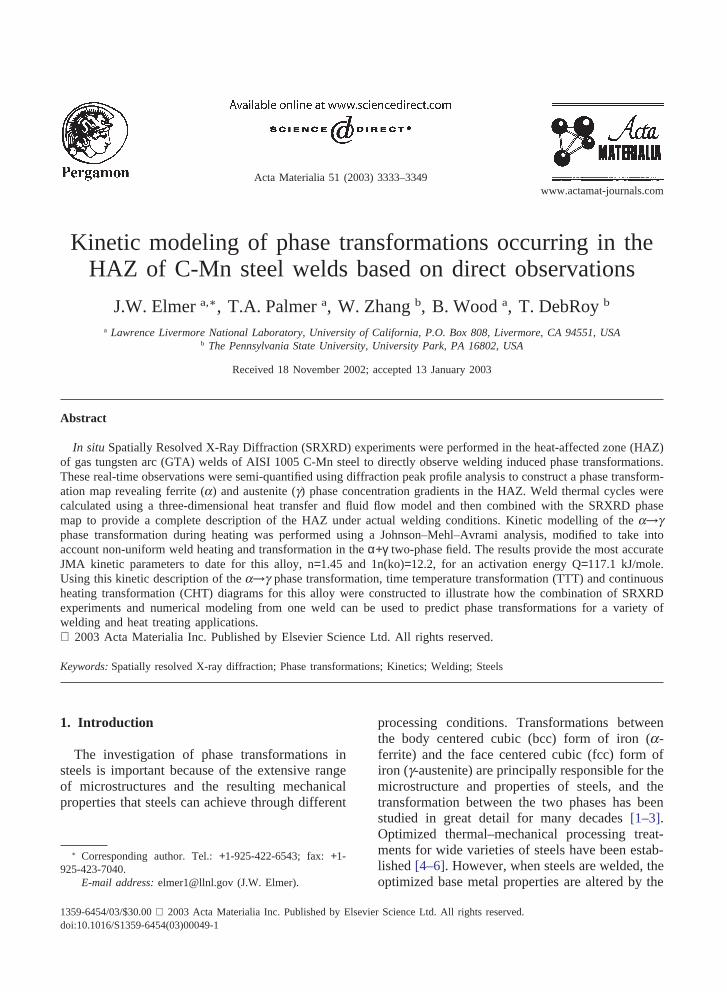
The internal consistency of these kinetic para-meters was checked by comparing the austenitefraction at the different SRXRD locationspresented in Table 2 to the values calculated usingthe non-isothermal kinetic Eq. (B8). Fig. 10 com-pares the results from seven different SRXRDlocations, denoted in the plot as symbols, with thecalculated values, shown as the solid lines. Theoverall agreement between the experimentallymeasured data and the calculated data is reason-able, especially when considering the wide rangeof heating rates experienced at these differentHAZ locations.


Fig. 10. Comparison between the calculated and SRXRDexperimental phase fractions of g at different monitoringlocations.

4.2. TTT and CHT diagrams for 1005 steelwelds during heating

There are two main types of transformation dia-grams that are useful in understanding transform-ation kinetics during welding: Continuous HeatingTransformation (CHT) and Continuous CoolingTransformation (CCT) diagrams. The first type ofdiagram can be used to predict the transformationsthat occur on the heating side of the weld and thelatter on the cooling side of the weld. Both types ofdiagrams can be related to the Time TemperatureTransformation (TTT) diagrams that are used tomeasure the rate of the transformation at a con-stant temperature.

Using the kinetic parameters from the precedingsection, TTT and CHT diagrams were constructedfor the a→g transformation in the 1005 steel, whilethe CCT diagram determination will be reservedfor future work. The following JMA-based kineticequation (see Appendix B) and various time-tem-perature profiles were used in this analysis:

f(ti)Fi

� 1�exp{�[k0 � exp��Q

RTi� � (�t (5)

� ti)]n}

For a TTT diagram, the isothermal relationshipscan be expressed as a function of the temperatureabove the A1 temperature as follows:

T(t) � TH (6)

where T is the temperature at a given time t, andTH is the constant transformation temperature.

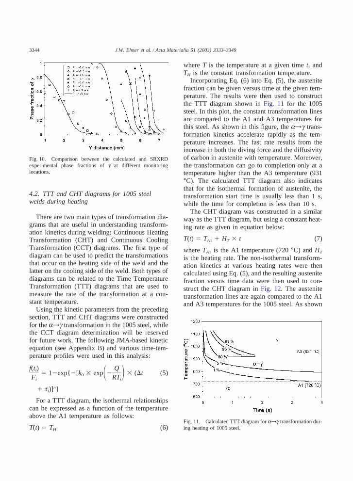
Incorporating Eq. (6) into Eq. (5), the austenitefraction can be given versus time at the given tem-perature. The results were then used to constructthe TTT diagram shown in Fig. 11 for the 1005steel. In this plot, the constant transformation linesare compared to the A1 and A3 temperatures forthis steel. As shown in this figure, the a→g trans-formation kinetics accelerate rapidly as the tem-perature increases. The fast rate results from theincrease in both the diving force and the diffusivityof carbon in austenite with temperature. Moreover,the transformation can go to completion only at atemperature higher than the A3 temperature (931°C). The calculated TTT diagram also indicatesthat for the isothermal formation of austenite, thetransformation start time is usually less than 1 s,while the time for completion is less than 10 s.

The CHT diagram was constructed in a similarway as the TTT diagram, but using a constant heat-ing rate as given in equation below:

T(t) � TA1 � HT � t (7)

where TA1 is the A1 temperature (720 °C) and HT

is the heating rate. The non-isothermal transform-ation kinetics at various heating rates were thencalculated using Eq. (5), and the resulting austenitefraction versus time data were then used to con-struct the CHT diagram in Fig. 12. The austenitetransformation lines are again compared to the A1and A3 temperatures for the 1005 steel. As shown

Fig. 11. Calculated TTT diagram for a→g transformation dur-ing heating of 1005 steel.


Fig. 12. Calculated CHT diagram for a→g transformationduring heating of 1005 steel.

in this figure, the transformation rate acceleratesrapidly with temperature, and both the start andfinish temperatures of the transformation increasewith increasing heating rate.

A comparison between Figs. 11 and 12 showsthat the time required for an equivalent amount ofaustenite transformation is longer under the CHTconditions than the TTT conditions. The reason forthis behavior is that the total kinetic strength of thetransformation is less for the CHT case than forthe TTT case, since the time temperature curvesare integrated up to the final temperature where thetransformation is predicted in the CHT conditions.The CHT diagram for the 1005 steel indicates thatfor the isothermal formation of austenite, the trans-formation start time is usually greater than 1 s,while the time for completion is greater than 10 s.In addition, it is apparent that some amount ofsuper heating is required to start and complete thephase transformation to austenite under non-iso-thermal conditions. For example, using a heatingrate of 50 °C/s, Fig. 12 predicts the transformationstart (1% austenite) to be 45 °C above the A1 tem-perature, while the transformation finish (99%austenite) is 135 °C above the A3 temperature.

Thus, using a combination of numerical weldmodeling to predict the weld temperature profiles,the SRXRD experimental data, and the JMA phasetransformation formalism, a CHT diagram hasbeen constructed for 1005 steel welds. This dia-gram allows the kinetics of the a→g transform-ation to be calculated over a relatively wide rangeof HAZ weld heating rates. It should be noted that

the kinetic parameters (k0 and n) calculated usingthe SRXRD data, and thus the CHT diagram,depend on the initial microstructure of the basemetal.

5. Conclusions

SRXRD phase mapping, numerical temperaturemodeling, and JMA kinetic calculations were per-formed to study the kinetics of the a→g phasetransformation in an AISI 1005 C-Mn steel. Thiscombination of experimental and modelingmethods provides previously unavailable insightinto this important phase transformation in theHAZ of C-Mn steels. Based on these results, anumber of specific conclusions can be made.

1. Diffraction peak analysis of the SRXRD datawas used to produce a semi-quantitative map ofthe phase transformations occurring in the weldHAZ. This work marks the first time that phasetransformations have been mapped in the HAZof a C-Mn steel weld. This data contains all theinformation necessary to evaluate weldinginduced phase transformations under real weld-ing conditions.

2. A three dimensional heat transfer and fluid flowmodel was used to predict the thermal gradientsaround the weld, and this information wasfurther used to develop and apply a numericalmodel based on a modified Johnson–Mehl–Avrami analysis that takes into account non-uni-form weld heating and transformation in thea + g two-phase field for the determination ofthe kinetics of the ferrite to austenite transform-ation during weld heating. Using the SRXRDexperimental data and an activation energyQ=117.1 kJ/mole, the JMA kinetic parametersfor the a→g phase transformation were determ-ined to be 1n(k0)=12.2, and n=1.45. These kin-etic parameters are consistent for a phase trans-formation controlled by diffusion of carbon withzero nucleation rate.

3. TTT and CHT diagrams were calculated for the1005 steel using the kinetic data determinedfrom the SRXRD experiments, providing agraphical means to predict the ferrite to austen-


ite transformation on weld heating for the 1005steel used in this investigation. These diagramsshow that a significant level of superheat isrequired for the initiation and completion of thephase transformation under the heating ratescommon to arc welding.

The a→g transformation represents only the firststep in the evolution of the weld HAZ microstruc-ture. After the complete transformation of themicrostructure to g, continued heating will resultin significant grain growth. Since grain size influ-ences the transformation kinetics, it is necessary,in the future, to incorporate a suitable grain growthmodel into the numerical weld modeling code topredict the austenite grain size distribution. Basedon this knowledge, a transformation model, suchas that developed by Bhadeshia et al. [33], can beincorporated into a comprehensive weld model andused to calculate CCT diagrams for this alloy. Sucha model will ultimately allow for the prediction ofHAZ microstructural evolution under a wide rangeof welding conditions.

Acknowledgements

This work was performed under the auspices ofthe US Department of Energy, Lawrence Liver-more National Laboratory, under Contract No. W-7405-ENG-48. We also acknowledge a grant, DE-FGO2-01ER45900, from the US Department ofEnergy, Office of Basic Energy Sciences, Divisionof Materials Sciences to The Pennsylvania StateUniversity. Portions of this research were carriedout at the Stanford Synchrotron Radiation Labora-tory, a national user facility operated by StanfordUniversity on behalf of the US Department ofEnergy, Office of Basic Energy Sciences. Theauthors would like to express their gratitude to Dr.Joe Wong of LLNL for assisting with the synchro-tron experiments, and Dr. Suresh Babu for assistingwith the data analysis and performing Thermocalccalculations. Finally, we wish to also express ourgratitude to Mr. Robert Kershaw of LLNL, whosadly passed away this year. Bob Kershaw perfor-med the optical metallography shown in this paperas well as all our other papers on this subject. His

outstanding metallographic expertise will be mis-sed by all of us who have worked with him overthe years.

Appendix A. SRXRD data conversion tovolume fraction austenite

In the conversion of the integrated intensities ofthe SRXRD diffraction peaks to volume fractionsof austenite and ferrite, there are several effectswhich must be taken into account. For example,the crystal structure and temperature are two fac-tors which affect the integrated intensity of eachobserved diffraction peak. These factors and othersare discussed in more detail in standard X-ray dif-fraction references [36]. The general methodologyused to convert the raw integrated intensities intothe volume fraction of each phase is given below.Where material parameters are required, the corre-sponding data for iron are used, since the AISI1005 C-Mn steel contains more than 99 wt. pct.iron.

The structure factor (F) enters into any scat-tering intensity calculation and increases the meas-ured peak intensity. This factor depends on theincident wavelength, the Bragg angle of the peak,and the atomic scattering factor and crystal struc-ture of the X-ray target. The amplitude of the scat-tered beam scales linearly with the amplitude ofthe complex structure factor, so the intensity of theresultant peak scales with its square. For bcc andfcc crystal structures, the squares of the structurefactor magnitudes are given by:

|F|2 � (4f)2 (bcc) (A1)

|F|2 � (2f)2 (fcc) (A2)

where f is the atomic scattering factor, estimatedby interpolation of a polynomial fit to tabulateddata for iron.

A factor accounting for the possibility of mul-tiple permutations of the Miller indices contribu-ting to a single reflection, thereby increasing themeasured intensity is considered next. The multi-plicity factor, p, is defined as the number of permu-tations of position and sign of ±h, ±k, ±l for planeswith the same interplanar spacing and structurefactor amplitude.


The systematic broadening of the peaks due tovarious geometrical considerations is next takeninto account. Three such considerations make upthe Lorentz factor: (1) a broadening and attenu-ation of all peaks due to the near-Bragg angle scat-tering, which scales to the theoretical peak inten-sities by a factor of (sin2q)�1, (2) the number ofplanes oriented at or around the Bragg angle is pro-portional to cosqand (3) the angular dependence ofthe energy density of the diffracted peaks, whichaffects the scattered intensity by a factor of(sin2q)�1.

Lorentz factor � � 1sin2q�(cosq)� 1

sin2q� (A3)

�1

4sin2qcosq

Combining this relationship with the polarizationdependence from the Thompson scattering formulaand neglecting a constant factor of 1/8, we obtainthe Lorentz–polarization factor:

Lorentz–polarization factor �1 � cos22qsin2qcosq

(A4)

Since the heat-affected zone is in a temperaturegradient, it is further necessary to incorporate atemperature factor describing the attenuation ofatomic scattering factors due to thermal vibrations:

Temperature factor � e�2M (A5)

In practice, the dimensionless quantity M is diffi-cult to calculate. However, the Debye approxi-mation, which is valid for pure elements possessinga cubic crystal structure, is used here. The cubiclattice is approximated as an isotropic continuumin which the vibration wave velocity is uniform,calculated as an average of the velocities of thetransverse and longitudinal modes [35]. Thisapproximation is quite good for temperaturesabove the Debye characteristic temperature, andsince the first allotropic transition upon heating inFe (a→a + g) occurs at 720 °C (993 K) and theDebye temperature of Fe is 430 K, its use here iseasily justified. Debye’s treatment gives the fol-lowing result:

M�6h2Tmk�2�f(x) �

x4��sinq

l �2

(A6)

where h is Planck’s constant, T is the absolute tem-perature, m is the mass of the vibrating atom(9.273 × 10�26 kg for Fe), k is Boltzmann’s con-stant, � is the Debye characteristic temperature ofthe substance in kelvins (430 K for Fe), x � � /T, and where

f(x) �1x�x

0

xex�1

dx (A7)

The relative intensity of each peak is given by thefollowing relation:

I � I0 /R (A8)

where I0 is the integrated area of the peak and thescaling factor, R, which includes the structure fac-tor, the multiplicity, the Lorentz–polarization fac-tor, and the temperature factor:

R � |F|2p�1 � cos22qsin2qcosq �e�2M (A9)

The austenite and ferrite volume fractions are cal-culated by dividing the sum of the phase-fractionscaled peak intensities for a given phase by thetotal of all phase-fraction scaled peak intensities ineach diffraction pattern.

Appendix B. Non-isothermal Johnson–Mehl–Avrami equation applicable to two-phaseequilibrium

In Eq. (3), the extent of the transformation fe(t)is related to the volume fraction of product phaseby the following equation:

fe(t) �f(t)F

(B1)

where f(t) is the volume fraction of product phaseafter time t, and F is the equilibrium fraction ofthe product phase at temperature T. For transform-ations of the eutectoid type, i.e. the transformationpath involves one phase transforming directly toanother at a constant temperature. In these typesof transformations fe(t) is identical to f(t) since Fis equal to 1. In many instances, such as the a-ferrite to austenite transformation during heating oflow carbon steels, the transformation path involves


a→(a + g)→g. In the a + g two-phase region, Fis not equal to 1 and can be calculated from thecorresponding phase diagram. Substituting Eqs. (4)and (B1) into Eq. (3), the isothermal JMA equationis rewritten as:

f(t)F

� 1�exp[�{k0 � exp��QRT� � t}n] (B2)

For eutectoid-type reactions, i.e. F = 1, the non-isothermal solution of the JMA equation has beenderived by Kruger [36]. However, Kruger’s formu-lation does not apply to systems where the trans-formation involves a two-phase region. Here, theJMA equation is extended to deal with such a two-phase region under non-isothermal conditions. Inthe following derivation, to simplify the problem,we assume that the kinetic parameters Q, k0, andn are independent of temperature, i.e. there is nosignificant change in the nucleation and growthmechanisms during the phase transformation [32].

During a non-isothermal solid-state transform-ation, the temperature changes continuously withthe time, i.e. T = T(t). In the following discussion,the non-isothermal kinetic equation will be derivedunder continuous heating conditions. The deri-vation procedure and the resulting equation are thesame for continuous cooling conditions. The con-tinuous change of the temperature with time canbe approximated by subsequent isothermal steps ofthe duration �t. The temperature–time curve startsat time t0 = 0 and temperature T1, and finishes attime tm = m�t and temperature Tm + 1. It should benoted that time equal to 0 is defined from theinstant the sample reaches the isothermal trans-formation temperature. This continuous curve isdiscretized into m isothermal steps. For example,the temperature between times ti�1 and ti is equalto Ti, and at the time ti, the temperature is changedfrom Ti to Ti + 1. This temperature (Ti + 1) prevailsbetween times ti and ti + 1.

The g fraction converted along the ith isothermaltime step (ti�1�t�ti)is expressed as:

f(t)Fi

� 1�exp{�[k0 � exp��Q

RTi� � (t (B3)

�ci)]n}

where Ti is the temperature at the ith step, Fi is the

equilibrium fraction of the new phase at tempera-ture Ti, and ci is a time used to account for the pre-converted fraction of new phase at the beginningof ith step. The term ci (c1 = 0) is determined fromthe continuity relation that the fraction calculatedusing Eq. (B3) at the beginning of the ith time stepis equal to that converted at the end of (i�1)th timestep, f(ti�1). Substituting t = ti�1 = (i�1)�t into Eq.(B3), we have:

ci � (i�1)�t�

n��ln�1�f(ti�1)

Fi�

k0 � exp��Q

RTi� (B4)

where �t is the time step.We can define the second term in Eq. (B4) as

another time constant ti (t1 = 0).0).

ti �

n��ln�1�f(ti�1)

Fi�

k0 � exp��Q

RTi� (B5)

Thus, we can obtain the fraction of new phase con-verted at the end of ith step by substituting t = ti

= i�t and ci = (i�1)�t�ti into Eq. (B3).

f(ti)Fi

� 1�exp{�[k0 � exp��Q

RTi� � (�t (B6)

� ti)]n} (1�i�m)

Eq. (B6) is the non-isothermal kinetic equationconsidering the equilibrium fraction of new phasein two-phase region. Further details of the deri-vation of Eq. (B6) are available elsewhere [37].

References

[1] Honeycomb RWK, Bhadeshia HKDH. Steels, microstruc-ture and properties. Metals Park (OH): American Societyof Metals, 1982.

[2] Jones S, Bhadesia HKDH. Metall Mater Trans A1997;28A(10):2005.

[3] Bhadeshia HKDH. Bainite in steels. 2nd ed. London: Insti-tute of Materials, 2001.

[4] Krauss GS. Steels: Heat treatment and processing prin-ciples. Materials Park (OH): ASM International, 1990.


[5] Vander Voort GF. Atlas of time-temperature diagrams forirons and steels. Materials Park (OH): ASM Inter-national, 1991.

[6] Harrison PL, Farrar RA. Int Mat Rev 1989;34(1):35.[7] Grong Ø. Metallurgical modelling of welding. London:

The Institute of Materials, 1994.[8] Easterling K. Introduction to the physical metallurgy of

welding. London: Butterworths and Co, 1983.[9] Ashby MF, Easterling KE. Acta Metall 1982;30:1969.

[10] Ion JC, Easterling KE, Ashby MF. Acta Metall1984;32:1949.

[11] Elmer JW, Wong J, Ressler T. Metall Mater Trans A2001;32A(5):1175.

[12] Zhang W, Elmer JW, DebRoy T. Scripta Mater2002;46:753.

[13] Zhang W, Elmer JW, DebRoy T. Mater Sci Eng A2002;333(1-2):320.

[14] Mundra K, DebRoy T, Kelkar K. Numer Heat Trans1996;29:115.

[15] Mundra K, Blackburn JM, DebRoy T. Sci Technol Weld-ing Joining 1997;2(4):174.

[16] Yang Z, DebRoy T. Metall Mater Trans B 1999;30B:483.[17] Pitscheneder W, DebRoy T, Mundra K, Ebner R. Welding

J 1996;75:71s.[18] Karpenko V, Kinney JH, Kulkarni S, Neufeld K, Poppe

C, Tirsell KG, Wong J, Cerino J, Troxel T, Yang J, HoyerE, Green M, Humpries D, Marks S, Plate D. Rev SciInstrum 1989;60:1451.

[19] Elmer JW, Wong J, Froba M, Waide PA, Larson EM.Metall Mater Trans A 1996;27A(3):775.

[20] Elmer JW, Wong J, Ressler T. Metall. Mater Trans A1998;29A(11):2761.

[21] Ressler T, Wong J, Elmer JW. J Phys Chem B1998;102(52):10724.

[22] Wong J, Froba M, Elmer JW, Waide PA. J Mat Sc1997;32:1493.

[23] Bearden JA, Burr AF. Rev Mod Physics 1967;39:125.[24] Palmer TA, Elmer JW, Wong J. Sci Tech Weld Join

2002;7(3):159.[25] Babu SS. Private communications, Oak Ridge National

Laboratory, 2000.[26] Sundman B, Jansson B, Andersson J. Calphad-Computer

Coupling of Phase Diagrams and Thermochemistry1985;9(2):153.

[27] Patankar SV. Numerical heat transfer and fluid flow.Hemisphere Pub Corp, 1980.

[28] Samuels LE. Optical microscopy of carbon steels.Materials Park (OH): American Society for Metals,1980 p.69.

[29] Speich GR, Demarest VA, Miller RL. Metall Trans A1981;12:1419.

[30] Nath SK, Ray S, Mathur VNS. ISIJ Inter 1994;34:191.[31] Askill J. Tracer diffusion data for metals, alloys and sim-

ple oxides. IFI/Plenum Press, 1970.[32] Christian JW. The theory of transformations in metals and

alloys, Part I. 2nd ed. Oxford: Pergamon, 1975.[33] Bhadeshia HKDH, Svensson LE. Modelling the evolution

of microstructure in steel weld metal. In: Easterling KE,Cerjak H, editors. Mathematical modeling of weldphenomena. London: Institute of Materials; 1993. p. 109.

[34] Cullity BD, Stock SR. Elements of X-ray diffraction. 3rded. Upper Saddle River (NJ): Prentice Hall, 2001.

[35] James RW. The optical principles of the diffraction of X-rays. Woodbridge (CT): Ox-Bow Press, 1982.

[36] Kruger PJ. Phys Chem Solids 1993;54:1549.[37] Zhang W, Elmer JW, DebRoy T. Modeling of Ferrite to

Austenite Transformation and Real Time Mapping ofPhases during GTA Welding of 1005 Steel, accepted forpublication in Trends in welding Research, Materials Park,(OH), ASM International, 2002.

kinetic modeling of phase transformations occurring in the ... · of gas tungsten arc (gta) welds...

Documents