kinetic modeling of gold nanoparticle formation by …
TRANSCRIPT

KINETIC MODELING OF GOLD NANOPARTICLE FORMATION
FOR RADIATION DOSE PREDICTION
by
Burak Akar
A thesis submitted in partial fulfillment
of the requirements for the degree
of
Master of Science
in
Chemical Engineering
MONTANA STATE UNIVERSITY
Bozeman, Montana
May 2017

©COPYRIGHT
by
Burak Akar
2017
All Rights Reserved

ii
ACKNOWLEDGEMENTS
I would first like to thank my thesis advisor Professor Jeff Heys of the Chemical
& Biological Engineering Department at Montana State University. The door to Prof.
Heys was always accessible whenever I ran into a trouble spot or had a question about
my research or writing.
I would also like to acknowledge by Professor Kaushal Rege and Karthik
Subramaniam Pushpavanam of the Chemical Engineering at Arizona State University.
They conducted the gold nanoparticle synthesis under ionizing radiation experiments and
provided the experimental measurements that are used in this thesis.
Burak Akar

iii
TABLE OF CONTENTS
1. INTRODUCTION ...........................................................................................................1
Gold NanoParticles ..........................................................................................................1
Radiation Detection ........................................................................................................3
Established Kinetic Models for Nanoparticle Formation ................................................5
2. METHODS FOR MODELING GNP FORMATION ...................................................11
The Finke-Watzky Model ..............................................................................................11
The Population Balance Model ......................................................................................14
Numerical Implementation ............................................................................................17
The Finke-Watzky Model ......................................................................................18
The Population Balance Model ..............................................................................20
Computational Cost ...............................................................................................23
3. RESULTS AND DISCUSSION ....................................................................................24
The Finke-Watzky Model ..............................................................................................24
The Population Balance Model ......................................................................................26
Model Sensitivity Analysis ....................................................................................30
4. CONCLUSION ..............................................................................................................33
Future Work ...................................................................................................................34
REFERENCES CITED ......................................................................................................35
APPENDICES ...................................................................................................................40
APPENDIX A: The Finke-Watzky Code (FW.py) ................................................41
APPENDIX B: The Population Balance Model Code (PBM.py)..........................45

iv
LIST OF FIGURES
Figure Page
1. Gold Nanoparticles Synthesized At Various Radiation Doses ............................5
2. LaMer Burst Nucleation ......................................................................................7
3. The Two Step Finke-Watzky Mechanism ...........................................................8
4. Particle Size Predictions of Two PBMs .............................................................10
5. FW Code, Differential Equations ......................................................................18
6. FW Code, Error and Conversion Functions .......................................................19
7. FW Code, Minimize Function ...........................................................................20
8. PBM Code, Define Bins ....................................................................................21
9. PBM Code, Individual Growth Coefficients .....................................................21
10. PBM Code, Differential Equations ..................................................................22
11. Computational Cost .........................................................................................23
12. FW Model, Precursor Prediction .....................................................................24
13. FW Model, Absorbance Predictions for All Doses .........................................25
14. PBM Model, Absorbance Predictions for All Doses .......................................26
15. PBM Model, Particle Distribution Predictions for All Doses..........................28
16. PBM Model Predictions as k1 Varies ..............................................................30
17. PBM Model Predictions as k2 Varies ..............................................................31
18. PBM Model Predictions as n Varies ................................................................32
v
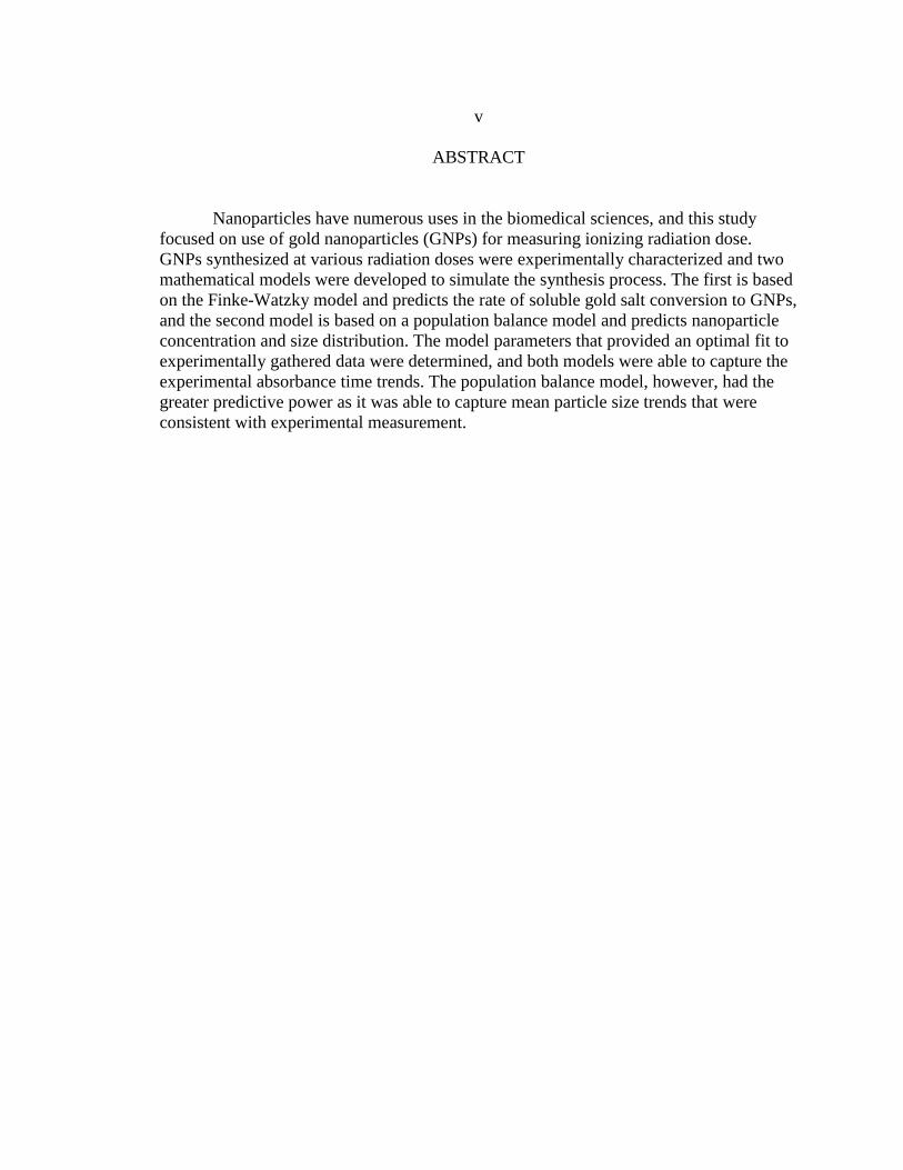
ABSTRACT
Nanoparticles have numerous uses in the biomedical sciences, and this study
focused on use of gold nanoparticles (GNPs) for measuring ionizing radiation dose.
GNPs synthesized at various radiation doses were experimentally characterized and two
mathematical models were developed to simulate the synthesis process. The first is based
on the Finke-Watzky model and predicts the rate of soluble gold salt conversion to GNPs,
and the second model is based on a population balance model and predicts nanoparticle
concentration and size distribution. The model parameters that provided an optimal fit to
experimentally gathered data were determined, and both models were able to capture the
experimental absorbance time trends. The population balance model, however, had the
greater predictive power as it was able to capture mean particle size trends that were
consistent with experimental measurement.

1
CHAPTER ONE: INTRODUCTION
Gold Nanoparticles
Nanoparticles have unique magnetic, optical, electronic, and catalytic properties,
which are related to their size and are different from the bulk material properties.
Colloidal suspensions of gold nanoparticles can display vibrant colors because gold
nanoparticles absorb and scatter light with incredible efficiency [1]. The solutions usually
have a red or blue/purple color based on particle size, shape and the local refractive
index. They have been used by artists for centuries. Gold and silver nanoparticles were
used to make the dichroic glass of the 4th-century Lycurgus Cup, which shows a different
color depending on whether or not light is passing through it; red when lit from behind
and green when lit from in front [2]. The process that was used to synthesize the
nanoparticles or the dichroic glass is not known, and the nanoparticles could even be an
accidental or unknown addition to the glass. Such an accidental discovery led to Michael
Faraday making some of the first scientific observations about gold nanoparticles. In
1856, Faraday accidentally created a ruby red solution while mounting pieces of gold leaf
onto microscope slides. Faraday started to further investigate the optical properties of the
colloidal gold. He prepared the first pure sample of colloidal gold and noted the light
scattering properties of suspended gold particles, which is now called the Faraday-
Tyndall effect [3].

2
Advanced microscopy methods, such as atomic force microscopy and electron
microscopy, have accelerated studies on gold nanoparticles. They were the subject of
several biomedical studies because many traditional biological probes such as antibodies,
lectins, superantigens, glycans, nucleic acids, and receptors can be attached to colloidal
gold particles [4]. There are now many potential innovative applications in numerous
fields such as biomedicine [5], electronics [6], catalysis [7], fuel cells [8], magnetic data
storage [9], agriculture [10], and solar cells [11].
Most gold nanoparticle synthesis methods involve reduction of chloroauric acid
(H[AuCl4]). Generally, a reducing agent is used on a solution of chloroauric acid to
reduce Au3+ ions to Au+ ions, which further reduce to Au0 atoms. The Au0 atoms are
significantly less soluble in aqueous solution, and they act as sites for the reduction of
more ions and they combine to form the first stable nuclei. Some sort of stabilizing agent
or a capping ligand that sticks to the nanoparticle surface is usually added to prevent the
particles from aggregating and to limit their growth. This synthesis was pioneered by J.
Turkevich [12], and his methods involved the reaction of small amounts of hot
chloroauric acid with small amounts of sodium citrate solution. The colloidal gold was
formed because the citrate ions act as both a reducing agent and a capping agent [13].
The method was refined by G. Frens but is still called the Turkevich method [14]. Most
synthesis methods follow a similar recipe to the Turkevich method but use different
reducing and capping agents as necessary to refine the synthesis process and produce
particles of different sizes and shapes [15, 16]. The gold solution can also be reduced
using radiolysis or gamma-irradiation [17, 18], potentially allowing the formation of gold

3
nanoparticles to be used for radiation detection and dosage measurement under the proper
conditions.
Radiation Detection
Ionizing radiation has several applications in nuclear power, medical imaging,
astrophysics, and medical therapy. When applied in a controlled fashion, ionizing
radiation can sterilize various products, including food produce, and kill cancer cells [19].
When released in uncontrolled fashion, ionizing radiation can induce either acute or
chronic reactions, it can cause harmful tissue reactions due to cells malfunctioning/dying,
cancerous tissue growth and, heritable diseases [20]. Given the potential benefits and
harms of using ionizing radiation, reliable and sensitive radiation detection is a key
component of harnessing the power and potential of ionizing radiation safely. Since
ionizing radiation can induce gold nanoparticle synthesis in a gold salt solution, which
causes a visible color change, such a solution could be used to detect and measure
radiation dose.
Currently there are a number of radiation dosimeters, available for detecting the
radiation exposure during medical and industrial processes. Electronic personal
dosimeters (EPD) are a common type of personal dosimeters for ionizing radiation, and
they can provide a live readout of radiation dose accumulation and sound alarms at
previously determined doses [21]. While they are useful in high dose areas, they can be
quite expensive. Another common device is the film badge dosimeter, but it is single use
only and uses a radiation sensitive silver film emulsion [22]. Though other dosimeter

4
materials that are less energy dependent and can more accurately assess radiation dose
from a variety of radiation fields with higher accuracy are available, film dosimeters are
still in use worldwide. Existing detection methods suffer from a number of limitations,
including difficulty of fabrication, high cost, low range of detection, and poor sensitivity.
Furthermore, these systems require secondary detection methods in several cases. For
example, film dosimeters require either densitometry or spectrophotometry to obtain
quantitative measurement of the doses [23, 24].
A detection method that uses a clearly visible color change in response to ionizing
radiation would be very useful in many fields since it does not require secondary
analyses. Existing colorimetric systems are based on several principles related to
radiation-induced chemical reactions and include Fricke or Fricke-like systems, which
are based on either oxidation or reduction metal ions, poly(methyl methacrylate) systems
(PMMA), and radiochromic dyes [23]. Fricke-like systems have detectable ranges from
1 to several hundred Grays, but typically require spectrophotometry for reading out the
chemical changes [23]. PMMA-based systems are excellent high-dose dosimeters with
ranges of 102 to 104 Gy [23]. Radiochromic dyes can be quite sensitive at detecting doses
from 10-1 up to 104, depending on dye species [23]. However, radiochromic dyes are
limited by their sensitivity to UV light as well as humidity [23]. Gold nanoparticle
synthesis through ionizing radiation can produce color change, thus solutions of gold ions
and templating agents can be used as colorimetric radiation detection systems. Figure 1
shows the effects of the templating agent and radiation dose on nanoparticle synthesis
rate.

5
Figure 1. Optical images of samples containing gold ions and different concentrations of
templating agents (C16TAB ) irradiated with a range of X-ray doses (Gy) (A) 2 mM, (B)
4mM, (C) 10mM, (D) 20mM, 2 hours post X-ray irradiation. The corresponding X-ray
radiation dose leading to the observed visual color change is indicated over each sample
in Gray (Gy).
Established Kinetic Models for Nanoparticle Formation
In order to produce a reliable dosimeter that utilizes nanoparticle formation, an
investigation of factors influencing nanoparticle formation is necessary. A large number
of factors such as the templating molecule, radiation dose, and initial soluble gold
concentration affect nanoparticle formation. A mathematical framework would enhance
the fundamental understanding of the mechanisms controlling nanoparticle formation
and, therefore, the efficacy of nano-bio sensing. A mathematical model would also permit
the investigation and optimization of parameters that enhance the sensitivity to ionizing
radiation, thus reducing the overall experimental burden.
6
The formation of nanoparticles is generally considered to be a two-step process
consisting of nucleation and growth. For many years, the process of the nucleation of
nanoparticles has been described through the LaMer burst nucleation, where the
monomer undergoes “burst nucleation”, the concentration of free monomers in the
solution decreases and nuclei are formed. The rate of this reaction is “effectively infinite”
and the reaction stops when the free monomer concentration gets too low [25-27]. While
this mechanism accounted for nucleation, growth was explained by Ostwald ripening or
particle coalescence. Ostwald ripening was first observed in 1900. The smaller particles
within the solution have higher a solubility and surface energy, and these particles
dissolve; in turn, allowing the larger particles to grow even more. The mathematical
theory of Ostwald ripening within a closed system is described by Lifshitz, Slyozov and
Wagner, the LSW theory [28, 29]. Digestive ripening is effectively the inverse of
Ostwald ripening. In this case, smaller particles grow at the expense of the larger ones.
This effect can also be influential in nanoparticle growth and has been described by Lee
et al. [27, 30]. Another way for the nuclei to grow is through collisions and coalescing
with other nuclei or clusters.
7
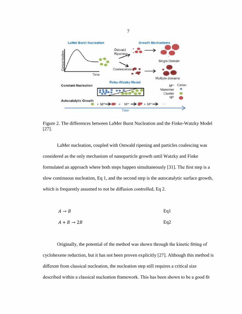
Figure 2. The differences between LaMer Burst Nucleation and the Finke-Watzky Model
[27].
LaMer nucleation, coupled with Ostwald ripening and particles coalescing was
considered as the only mechanism of nanoparticle growth until Watzky and Finke
formulated an approach where both steps happen simultaneously [31]. The first step is a
slow continuous nucleation, Eq 1, and the second step is the autocatalytic surface growth,
which is frequently assumed to not be diffusion controlled, Eq 2.
𝐴 → 𝐵 Eq1
𝐴 + 𝐵 → 2𝐵 Eq2
Originally, the potential of the method was shown through the kinetic fitting of
cyclohexene reduction, but it has not been proven explicitly [27]. Although this method is
different from classical nucleation, the nucleation step still requires a critical size
described within a classical nucleation framework. This has been shown to be a good fit

8
for many systems including iridium [32], [33], platinum [34], ruthenium [35] and
rhodium [35].
Figure 3. The Two step Finke-Watzky mechanism [36].
There have been several studies on the Finke-Watzky model. Georgiev et al.
explored the use of atomic force microscopy (AFM) for examining gold nanoparticle
growth [32]. The gold nanoparticles were obtained using Turkevich synthesis at two
different temperatures. AFM images taken during growth were analyzed to obtain
nanoparticle sizes and to compare the data with dynamic light scattering and transmission
electron microscopy measurements. They used a two-step Finke-Watzky kinetic model to
fit their spectroscopy data and calculated the corresponding kinetic constants for
chemically synthesized gold nanoparticles [32].

9
The Perala study examined the two-step mechanism for iridium nanoparticles. It
expands on the Finke-Watzky mechanism to produce several population balance models
(PBM) that predict particle size based on different assumptions about the formation
process [36]. Their first population balance model makes the assumption that the growth
rate is proportional to particle volume, but their results are more polydisperse than
desired. In their experiments, they found that nucleation becomes negligible after the
initial induction period, which results in a very monodisperse population. Their second
PBM aimed at challenging one of their initial assumptions, and this time they assumed
that the growth rate was proportional to surface area. The polydispersity of the modeled
result did not improve, unfortunately. They note that one of the ways to make nucleation
a negligible process while particle growth continues is to make the former depend on
another species. They divided the nucleation step into two steps in order to simulate an
intermediate species. They created two more PBMs that tested this alternative synthesis
route, the second one assumed second-order dependence on the intermediate species. The
new models still did not predict the polydispersity adequately well, and the precursor
consumption did not fit as well anymore. However, their analysis of those models
revealed that a mechanism that seeks to explain their experimental observations must
decrease the time window over which nucleation occurs, by delaying the onset of
nucleation. They used a form already available in the literature for nucleation rate with
delayed onset of nucleation [36, 37]. Their final model predicts the observed nucleation
window correctly. They conclude that the two step mechanism does not capture particle
synthesis correctly and out of all the models they investigated, the delayed onset of
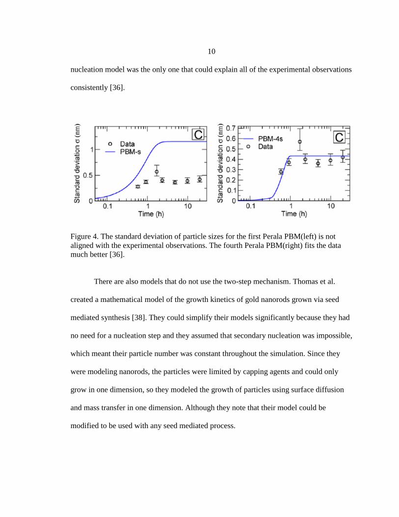
10
nucleation model was the only one that could explain all of the experimental observations
consistently [36].
Figure 4. The standard deviation of particle sizes for the first Perala PBM(left) is not
aligned with the experimental observations. The fourth Perala PBM(right) fits the data
much better [36].
There are also models that do not use the two-step mechanism. Thomas et al.
created a mathematical model of the growth kinetics of gold nanorods grown via seed
mediated synthesis [38]. They could simplify their models significantly because they had
no need for a nucleation step and they assumed that secondary nucleation was impossible,
which meant their particle number was constant throughout the simulation. Since they
were modeling nanorods, the particles were limited by capping agents and could only
grow in one dimension, so they modeled the growth of particles using surface diffusion
and mass transfer in one dimension. Although they note that their model could be
modified to be used with any seed mediated process.

11
CHAPTER TWO: METHODS FOR MODELING GNP FORMATION
Gold nanoparticles were synthesized at various radiation doses and the
absorbance and mean particle size were measured. The analysis of the measurements
showed that as the radiation dose increased, the concentration of synthesized GNPs
increased and the diameter of GNPs decreased. Because of the extremely short time scale
of the water radiolysis and gold ion reduction reactions, the reduction reactions are not
included explicitly in either of the mathematical models described below, and, instead,
the initial concentration of zero valence gold atoms is calculated using experimental
measurements of absorbance and particle size at different radiation doses. All models
assume that Ostwald ripening, digestive ripening and collisions with other particles have
negligible effects on particle growth. Two different mathematical models are examined
here that predict the formation of GNPs at low radiation doses such as those needed for
practical radiation dose measurement.
The Finke-Watzky Model
The first kinetic model describing the formation of gold nanoparticles begins with
a reaction describing the formation of stable gold nanoparticle nuclei:
𝐴𝑘1→𝐵 Eq.3
where 𝐴 is the concentration of gold atoms, 𝐵 represents the total amount of gold in
relatively stable nanoparticle nuclei and 𝑘1 is the forward rate of nanoparticle nuclei

12
formation. The stable nuclei formation step is often the slow step in nanoparticle
synthesis. The second reaction in the Finke-Watzky model describes the growth of stable
nuclei through the incorporation of additional gold atoms:
𝐴 + 𝐵𝑘2→ 2𝐵.
Eq.4
The Finke-Watzky model ultimately predicts the rate at which insoluble gold
atoms, 𝐴, are assimilated into gold nanoparticles, 𝐵. However, a significant limitation of
the Finke-Watzky model is that it does not predict either nanoparticle size or the
concentration of particles.
The main prediction of the model, the total moles of gold atoms cumulatively
contained in all the particles as a function of time, is converted to an estimate of
absorbance using experimental measurements of average particle size so that the model
prediction can be compared with the experimental measurements taken using UV-vis
spectrometry. The following equation (Beer’s Law) was used to convert the model
prediction of particle concentration to absorbance [39]:
𝐴 = 휀𝑏𝐶 Eq.5
where, 𝑏 is path length (i.e., the distance of the path that the light travels through the
sample), 휀 is the extinction coefficient, and 𝐶 is the particle concentration. The particle

13
concentration was calculated by dividing the total concentration of gold atoms in particle
form by the mean particle volume:
𝐶 =
𝐵43𝜋𝑟3𝑁𝐴𝑀𝐴𝑢
Eq.6
where, 𝑁𝐴 is the Avogadro’s number and 𝑀𝐴𝑢 is the molar density of gold, 98 𝑚𝑜𝑙𝐿
. The
diameters of the nanoparticles synthesized under different radiations were measured
experimentally, and for the Finke-Watzky model, all synthesized particles were assumed
to be the measured mean particle size. The extinction coefficient is also dependent on the
particle size and is calculated using:
ln 휀 = 𝑘 ∗ ln𝐷 + 𝑎 Eq.7
where, 𝐷 is the particle diameter and, 𝑘 and 𝑎 are constants that were calculated
previously to be 3.32111 and 10.80505 for gold nanoparticles [39].

14
The Population Balance Model
Population balance models explicitly model particles of different sizes and allow
prediction of growth based on size. The governing population balance equation is given
by:
𝜕𝐵(𝑟)
𝜕𝑡+𝜕
𝜕𝑟[𝜇(𝑟)𝐵(𝑟)] = 𝑁 ⋅ 𝛿(𝑟 − 𝑟𝑐) Eq.8
where 𝐵(𝑟) is the population of particles of size 𝑟, 𝜇(𝑟) is the growth rate for particles of
size 𝑟, and 𝑁 is the nucleation rate of particles of critical radius size, 𝑟𝑐. The
implementation of particle balance models is frequently achieved by discretizing particles
of different sizes into different size groups with each group representing a specific radius
range. As a result, nanoparticle growth is split into numerous reactions that each describe
the growth of particles in radius range 𝑖 and, after sufficient time, these particles grow into
radius range 𝑖 + 1. In other words, when the particles reach a certain size, they move into
a grouping of larger sized particles. Population balance models use the following reactions
for nucleation and growth after discretizing particles into various size groups:
𝐴𝑘1→𝐵0
Nucleation Eq.9
𝐴 + 𝐵𝑖𝑘2,𝑖→ 𝐵𝑖+1
Growth Eq.10

15
where, 𝐵0 is the concentration of stable gold nanoparticle nuclei and 𝐵𝑖 is the concentration
of nanoparticles in size range 𝑖. The smallest stable nuclei (𝐵0) are assumed to consist of
approximately 20 atoms [36], which is used to calculate the minimum radius of the
particles. The maximum particle radius is estimated from experimental measurements, and
the range of possible particle radii is divided into 𝑁 discrete groups. The growth reaction
leads to particles of slightly larger size, and particles continue to grow at different rates
(given below) until the maximum particle radius of 69 nm is reached (𝑁 = 50 for current
model). A critical issue associated with population balance models is the determination of
the growth rate, 𝑘2,𝑖, which is often a function of particle size.
Material balances on the nucleation and growth reactions result in a model
consisting of the following system of differential equations:
𝑑𝐴
𝑑𝑡= −𝑘1 ⋅ 𝐴
𝑛 −∑ 𝑘2,𝑖 ⋅ 𝐴 ⋅ 𝐵𝑖
𝑁−1
𝑖=0
Eq.11
𝑑𝐵0𝑑𝑡
= 𝑘1 ⋅ 𝐴𝑛 − 𝑘2,0 ∗ 𝐴 ⋅ 𝐵0 Eq.12
𝑑𝐵𝑖𝑑𝑡= 𝑘2,𝑖−1 ⋅ 𝐴 ⋅ 𝐵𝑖−1 − 𝑘2,𝑖 ⋅ 𝐴 ⋅ 𝐵𝑖 for 𝑖 = 0, 1, … ,𝑁 Eq.13
𝑑𝐵𝑁𝑑𝑡
= 𝑘2,𝑁−1 ⋅ 𝐴 ⋅ 𝐵𝑁−1 Eq.14
The exponent, 𝑛, is an unknown parameter that will be determined using the
experimental data. Mathematical models of similar systems have used 𝑛 = 1 to 4 [40].
16
Therefore, values over that range are initially considered here. These equations were non-
dimensionalized before obtaining a numerical approximation of the solution.
For some systems, the growth rate is controlled by the association rate of new
monomer (i.e., reaction rate limited systems) while in other systems, the growth rate is
controlled by the diffusion of gold atoms to the nanoparticle surface (i.e., diffusion limited
systems) [27, 41]. If 𝐼 is defined as the molar flux of gold to the surface of the nanoparticle
and 𝑉𝑀 is the molar volume, then the change in particle volume and radius is:
𝐼 =
1
𝑉𝑀
𝑑𝑉
𝑑𝑡=4𝜋𝑟2
𝑉𝑀
𝑑𝑟
𝑑𝑡 . Eq.15
The total flux of molecules to the surface is proportional to particle radius (i.e., the
characteristic diffusion length scale) for the diffusion limited case (i.e., 𝐼 = 4𝜋𝑟𝒟(𝐶𝑏 −
𝐶𝑠𝑢𝑟𝑓𝑎𝑐𝑒), and the total flux is proportional to particle surface area for the reaction limited
case (i.e., 𝐼 = 4𝜋𝑟2𝑘𝐶𝑠𝑢𝑟𝑓𝑎𝑐𝑒). For the diffusion limited case, the rate at which particles
are predicted to move from one size group, 𝐵𝑖, to the next group, 𝐵𝑖+1, is inversely related
to the particle radius because 𝑑𝑟
𝑑𝑡=𝑉𝑀
𝑟⋅ 𝒟(𝐶𝑏 − 𝐶𝑠𝑢𝑟𝑓𝑎𝑐𝑒). For the reaction rate limited
case, 𝑑𝑟
𝑑𝑡= 𝑉𝑀𝑘𝐶𝑠𝑢𝑟𝑓𝑎𝑐𝑒. Experimental data from the system of interest here suggested that
the growth rate of the nanoparticles was dependent on particle size (i.e., the system was
diffusion limited) so the particle grow rate, 𝑘2,𝑖, was set to decrease as the particle radius
increases:

17
𝑘2,𝑖 =
𝑘2𝑜
𝑟𝑖 Eq.16
where 𝑘2𝑜 is an unknown growth rate constant. The population balance model predicts
both the rate of nanoparticle formation but also the size distribution of the final
population of nanoparticles.
The results of the model, the concentrations of particles of certain sizes, are
converted to estimate of absorbance so that they can be compared with the experimental
measurements taken using UV-vis spectrometry. Equations 5 and 7 were used to convert
concentration to absorbance. For equation 7, particles in the same size group were
assumed to have the same diameter and particles were assumed to grow in discrete
amounts.
Numerical Implementation
Algorithms to numerically solve the system of ordinary differential equations
associated with each model were developed and implemented using Python and the Scipy
libraries. The initial value problems were solved using ODEPACK from Lawrence
Livermore National Laboratory [42]. The initial conditions were set by assuming that no
nanoparticles were present at the start of the simulation, and the initial concentration of
insoluble gold atoms was set based on experimental measurements at various radiation
doses. Finally, for both models, the unknown reaction rates (𝑘1, and 𝑘2 for Finke-Wazky
and 𝑘1 and 𝑘2𝑜 for the population balance model) were determined by minimizing the 𝐿2-

18
norm of the difference between experimental measurements and model prediction using
either a Nelder-Mead simplex algorithm or manual parameter adjustment.
The Finke-Watzky Model
This simple model solves two differential equations, that describe nucleation and
growth, for four hours (see algorithm in figure 5). The defined function “NucGrowth1”,
describes the set of differential equations that are derived from equations 5 and 6. The
function requires an input of a vector ‘C’, that denotes the current particle concentrations
for every size bin and a vector ‘t’, that represents the current simulated time. The reaction
coefficients are specified as parameters, so that they can be varied to search for the
optimal values.
Figure 5. “NucGrowth1” describes the set of differential equations that are derived from
equations 5 and 6.
The results of the integration are particle concentrations for various sized
particles, these are converted to absorbance by the function ‘Absorbance.’ The
conversion is based on equations 5, 6 and 7, so that the concentrations can be compared
Tm=numpy.array([0,0.1,0.25,0.5,0.75,1,1.5,2,2.5,3,3.5,4])
def NucGrowth1(C,t,param):
k1=param[0]
k2=param[1]
A=C[0];
B=C[1];
dAdt=-k1*A**n-k2*A*B
dBdt=k1*A**n+k2*A*B
return numpy.array([dAdt,dBdt])

19
against the experimental data. As seen in figure 6, the “Absorbance” function requires a
vector that contains concentration over time and particle diameters as inputs. The
function ‘Error’ requires the experimental absorbance measurements and the simulated
absorbance values at the same time points as inputs and calculates the difference between
the model prediction and the experimental data. The function “runSim” executes the
previously described functions and computes their outcome based on the two parameters,
the reaction coefficients. The scipy.integrate library is used to solve the differential
equations.
Figure 6. “Absorbance” converts gold concentration to the absorbance of gold
nanoparticles. ‘Error’ compares the experimental Absorbance values with the model.
“runSim” executes the previously described functions.
def Absorbance(S,D):
E=math.exp(3.32111*math.log(D)+10.80505)
atoms_per_particle=Na*AuM*(4/3*math.pi*((1e-8)*D/2)**3)
C=(S[:,1])/atoms_per_particle #M
A=C*E
return A
def Error(S,Abs):
error=0
for i in range (numpy.size(Abs)):
error += (S[i]-Abs[i])**2
return numpy.sqrt(error)
def runSim(param):
S=odeint(NucGrowth1,iC,Tm,args=(param,))
A=Absorbance(S,D)
error = Error(A,Abs)
print error,param[0],param[1]
return(error)

20
The difference between the model predictions and the data is calculated and
minimized over several iterations of the code, while varying the two parameters, the
reaction coefficients 𝑘1 and 𝑘2. Each time the code is run, the parameters are modified to
determine new values that provide better agreement between the model prediction and the
experimental data. After optimal parameter values are determined, they need to be
inserted manually into the code. The scipy.optimize library was used to minimize the
error.
Figure 7. The minimize command calculates the parameters that provide the closest
results to the experimental data.
The Population Based Model
This model describes the growth of the particles using 50 successive ordinary
differential equations, which represent balances on different particle size ranges. All the
particles are assumed to have a radii between 0.5 nm (the smallest stable size) and 70 nm
(the largest size observed experimentally in this system), and this radius range is
separated into 50 size groups called bins. The differential equations describe the rates at
which the particles change size groups. The minimum and maximum particle sizes were
chosen based on experimental measurements. The constant parameter, ‘nucleus’ is set so
that the smallest nuclei consist of 20 atoms. The function “atoms_bin” calculates the
atoms required for a particle to transfer from one size group to the next, the only input
necessary is the bin number.
error = runSim(kparams)
print error
minimize(runSim,kparams,bounds=((0,None),(0,None)))

21
Figure 8. The experimentally determined range of possible particle radii is divided into
50 ‘bins’, and the function “atoms_bin” calculates the size of each bin.
It was assumed that the growth rate constant, 𝑘𝑖,2, decreases as the particle size
increases. The function “growth”, calculates an individual growth rate constant for each
size group. As seen in figure 9, the individual growth rates are based on an unknown
constant and are inversely proportional to particle size and the gold atoms necessary for
growing to the next size.
Figure 9. The function “growth” calculates an individual growth rate constant for each
size group.
The function “df1” describes the system of differential equations to be solved and
it requires the current particle concentration vector, ‘N’, the simulation time, ‘t’, and the
kinetic rate parameters, ‘params’, as inputs. As seen in figure 10, these equations are non-
dimensionalized using the function “atoms_bin” and the constant defined as ‘nucleus’.
The function “Atotal” describes the equations that convert particle concentration to
bins = 50
max_radius = 6.91875e+1 #nm
min_radius = 5.0e-1 #nm
radius_bin = (max_radius-min_radius)/(bins-1) #nm
nucleus=20
def atoms_bin(bin_num):
V_bin=(4.0*math.pi/3.0)*(((min_radius+bin_num*radius_bin)**3)-
((min_radius+(bin_num-1)*radius_bin)**3)) #nm^3
atom_bin=(V_bin*(1e-24))*(Na*AuM)
return atom_bin
def growth(bin_num, params):
k2=params[1]
radius = min_radius+(bin_num-1)*radius_bin
return k2 / ((radius)*atoms_bin(bin_num))

22
absorbance based on particle size and sums the absorbance of all the particles for each
timestep; it only requires a matrix of concentration at different time points as input.
Figure 10. The function that describes the system of differential equations to be solved,
“df1” and the function that converts particle concentrations over time to absorbance over
time, “Atotal”.
The current simulation code runs the simulation 6 times, once for each unique
radiation dose, and calculates the particle size distributions which are compared with the
experimental distributions. The minimize function could not be used in conjunction with
this code due to the high computational cost for a single set of parameters. Instead,
def df1(N, t, params):
n=4
k1=params[0]
dNdt = numpy.zeros(bins,dtype=numpy.float)
dNdt[0] = -k1*N[0]**n - growth(1, params)*N[0]*N[1]
dNdt[1] = k1*((N[0]**n)/nucleus) - growth(1,params)*N[0]*N[1]/atoms_bin(1)
for i in range(2,bins-1):
dNdt[0] = dNdt[0] - growth(i,params)* N[0]*N[i]
dNdt[i] = growth(i-1, params)*N[0]*N[i-1]/atoms_bin(i-1) -
growth(i,params)*N[0]*N[i]/atoms_bin(i)
dNdt[bins-1] = growth(bins-2,params)*N[0]*N[bins-2]/atoms_bin(bins-2)
return numpy.array(dNdt)
def Atotal(C):
(m,n)=numpy.shape(C)
Atot=numpy.zeros(m)
for i in range (0,m):
for j in range (0,n):
if C[i,j]<0:
C[i,j]=0
radius = min_radius+(j)*radius_bin
Atot[i]+=1*(C[i,j]*1e-6)*math.exp(k*math.log1p(radius*2)+a
return numpy.array(Atot)

23
optimal parameter values were determined by manually testing various parameter values
to obtain the best possible agreement with the experimental data.
Computational Cost
The process time of the simulation was recorded using the
“time.process_counter()” command. For this measurement, an Alienware laptop with
Intel Core© i7-6820HK CPU @2.70GHz processor and 8.00 GB RAM was used. Figure
11 shows the processing time increase as the number of bins increases. The empirical
data suggests that the process time has the following relation to the number of unique
particle size bins:
t = 0.0068n2 + 0.3969n - 0.699
Eq.16
Figure 11. Process time (seconds) versus number of bins.
0
50
100
150
200
250
0 25 50 75 100 125 150
Pro
cess
Tim
e (s
eco
nd
s)
Number of Bins

24
CHAPTER THREE: RESULTS AND DISCUSSION
The Finke-Watzky Model
The Finke-Watzky model prediction for the conversion of gold atoms into gold
nanoparticles using optimal values for the reaction rates so that the model predictions
match the experimental data are shown below in Figure 12. The experimental data shown
in Figure 12 is from experimental measurements of absorbance after exposure to a radiation
dose of 15 Gy. The initial gold salt concentration is 0.0109 mM and size measurements
show that the mean particle diameter is 88.46 nm. Under these conditions, the optimal
values for the kinetic parameters, 𝑘1, and 𝑘2, are 1 min-1 and 3 ∗ 105 min-1M-1,
respectively.
Figure 12. The Finke -Watzky model prediction for the precursor concentration and the
absorbance of gold- nanoparticles over time for 15 Gy radiation dosage.

25
Figure 13, shows how the same kinetic parameters that provided the best fit for
the median dosage, 15 Gy, fit the model to experimental data at other radiation dosages.
Unfortunately, this model does not predict the size distribution of the nanoparticles so
comparisons with nanoparticle size measurements are not possible. The model
predictions are least accurate for the 5 Gy case where GNP formation is predicted to
occur more rapidly that is observed experimentally. Overall, however, the model
agreement with the experimental data is good.
Figure 13. The absorbance predictions for various radiation doses.

26
The Population Balance Model
The next set of results are based on the population balance model. Figure 14 shows
the model prediction of absorbance versus time for a range of different radiation doses from
5 to 35 Gy. The kinetic parameters, 𝑘1, and 𝑘2, are 8 ∗ 10−10 min-1 and 3 ∗ 1013 m4min-
1µM-1, respectively, and 𝑛 is set to 4. Unfortunately, the earliest experimental
measurements of absorbance are 60 minutes after the radiation dose was delivered so the
initial rate of change in absorbance cannot be compared between the model and the
experimental data.
Figure 14. Absorbance versus time(min) for different radiation doses (Gy).

27
The agreement between the model predictions and the experimental
measurements is the strongest at radiation doses of 15 Gy or higher, and the agreement is
weakest at the 5 Gy dose. This discrepancy is probably due to the slower than actual
nucleation rate used in the model, but could also be due to error in the measurement of
the initial, reduced gold atom concentration, i.e., the initial concentration of 𝐴𝑢0. The
initial concentration is determined by first measuring the gold salt concentration (i.e., the
𝐴𝑢3+ concentration) and then measuring soluble gold concentration after radiation
exposure (i.e., measuring the 𝐴𝑢3+ that was not converted to 𝐴𝑢0 by radiation exposure).
At the lower radiation doses (5 and 10 Gy), less of the gold salt was converted to 𝐴𝑢0 and
this smaller quantity could be more difficult to accurately determine. Hence, the
experimental error in measuring the initial 𝐴𝑢0 concentration is most likely greatest for
the lowest radiation doses, and this error could help explain the differences between the
experimental measurements and model predictions seen in Figure 14.
Figure 15 shows the model prediction for the final particle size distribution for
different radiation doses using the same model parameters as Figure 14. The vertical,
dashed lines represent the experimental measurements of median particle size for the
various radiation doses. The model predictions agree with the experimental observation
that the mean particle size decreases as the radiation dose is increased. For higher radiation
doses, there is a higher initial concentration of 𝐴𝑢0 atoms and the formation of the smallest
stable nanoparticles (i.e., nucleation) is more rapid. The numerous small nanoparticles
quickly grow, but all the 𝐴𝑢0 in the solution is consumed before the particles are very large
(i.e., when they are still only 35-40 nm). Conversely, at lower radiation doses, the smaller

28
𝐴𝑢0 concentration results in less nucleation and fewer nanoparticles, overall. Even though
the 𝐴𝑢0 concentration is lower, the small number of nanoparticles allows the particles to
grow much larger before the 𝐴𝑢0 concentration drops to very low levels.
Figure 15. The particle concentration versus simulated particle radius at varying radiation
doses (Gy). Higher radiation doses result in more abundant but smaller particles.
The agreement between the model and the experimental measurements is best at
the middle radiation doses (15 and 25 Gy), but in the largest radiation doses, the model
prediction is for larger particles than what was measured experimentally. One possible
explanation for this is that the model includes a maximum particle size that cannot be
exceeded. If a few experimental particles exceed this maximum particle size (an event
that almost certainly occurred), then less 𝐴𝑢0 was available for particle growth in the

29
experiment than in the corresponding model prediction. As a result, most of the
experimental particles would be slightly smaller than predicted by the model because a
few particles are much larger than predicted by the model.
Another possible explanation for the larger particles predicted by the model is that
the model assumed diffusion was limiting the particle growth rate so that the rate
constant, 𝑘𝑖,2, was inversely related to the particle radius. This is only a 1-dimensional
approximation of the diffusion limitation effects, and a full diffusion model for each
particle could reveal an even greater change in the rate constant as the particle radius
increases, thus leading to greater slowing of the growth of particles at high concentrations
(i.e., high Gy) and reducing the mean particle size predicted by the model.
One more explanation for the smaller particles observed experimentally is that the
nucleation rate is faster than modeled, especially for the highest radiation doses. The
nucleation rate is proportional to 𝐴4, or the reduced gold atom concentration [𝐴𝑢0]4.
This implies that a doubling of the initial 𝐴𝑢0 concentration results in a nucleation rate
that is 16-times faster. Using a non-integer exponent (e.g., 4.5) could result in slightly
faster nucleation and the more abundant particle number would limit particle size
providing better agreement between the model the experimental data.

30
Model Parameter Sensitivity Analysis
Figure 16 shows how the results of the PBM model are affected by changes in the
nucleation rate, 𝑘1. Halving the nucleation rate to 4×10⁻¹⁰ min-1, decreases the initial
slope of the absorbance predictions while increasing the particle sizes. As expected,
slower nucleation leads to fewer initial nuclei to be formed, leaving behind more
precursor to be used for growth. This results in a slower increase in Absorbance and
decreased particle concentrations for all radiation doses. The leftover precursor allows the
particles to grow bigger, creating fewer but larger particles. Doubling the nucleation rate
to 1.6×10⁻⁹ min-1, has the opposite effects. Faster nucleation leads to more nuclei, which
results in a faster increase in Absorbance and increased particle concentrations for all
radiation doses. The production of extra nuclei consumes precursor and limits the growth
of the particles, creating more but smaller particles.
Figure 16. The absorbance and particle distribution predictions of the PBM model with
A) half the nucleation rate and B) double the nucleation rate.

31
Figure 17 shows how the results of the PBM model are affected by changes in the
growth rate, 𝑘2. Halving the growth rate to 1.5×10¹³ m4min-1µM-1, decreases the initial
slope of the absorbance predictions while also decreasing the particle sizes. As expected,
slower growth allows more initial nuclei to form, leaving less precursor for growth. This
results in a slightly slower increase in Absorbance and increased particle concentrations
for all radiation doses. The production of extra nuclei consumes precursor and limits the
growth of the particles, creating more, smaller particles. Doubling the growth rate to
6×10¹³ m4min-1µM-1, has the opposite effects. Faster growth leads to fewer nuclei
having a chance to form before all the precursor is consumed. The result is a more rapid
increase in Absorbance, decreased particle concentrations, and larger particles for all
radiation doses.
Figure 17. The absorbance and particle distribution predictions of the PBM model with
A) half the growth rate and B) double the growth rate.

32
The particle distributions are a result of the nucleation and growth reactions
competing for precursor. The exponent on the precursor concentration in the nucleation
reaction, 𝑛, increases the rate at which nucleation occurs, and more rapid nucleation
generates more competition with the growth reaction for the limited supply of precursor.
Figure 17, shows the effect of changing the precursor consumption power on the GNP
size distribution.
Figure 18. The particle distribution as the precursor consumption power, n, is increased.
For the case of slower nucleation, 𝑛 = 1, higher radiation doses always result in
larger particles because higher radiation doses create more precursor and the additional
precursor results in larger GNPs. This result directly contradicts what is observed
experimentally. For the 𝑛 = 2 and 𝑛 = 3 cases, nucleation is more rapid, especially at
the higher radiation doses, so we start to see the highest doses generating smaller
particles because of precursor depletion, but the particle sizes at different radiation doses
are still less variable than what was observed experimentally. The optimal agreement
with the experimental measurements is 𝑛 = 4, as shown in Figure 15.

33
CHAPTER FOUR: CONCLUSIONS
Mathematical models of gold nanoparticle formation kinetics following radiation
exposure were developed and compared to experimental measurements of absorbance
and particle size. The first mathematical model was based on the Finke-Watzke model.
The model is relatively simple to implement and parameter optimization using
experimental data is straightforward. Unfortunately, model agreement with the
experimental system of interest here was only optimal for one radiation dose, and the
model parameters needed to be changed for other radiation doses to retain a high quality
fit with the data. The greatest limitation of the Finke-Watzke model is that it only
predicts the precursor consumption rate and it does not predict the final particle size
distribution.
The second mathematical model developed here was based on a population
balance model. This model is more difficult to implement and has greater computational
requirements. The model prediction of absorbance at different radiation doses was good
for the lower doses, but there was less agreement at the highest doses. The particle size
distribution prediction was consistent and often very close to the experimental
measurements. For all radiation doses, the model predicted a larger mean particle size
than was observed experimentally, and some possible explanations for this discrepancy
were given the results and discussion section.

34
Future Work
The mathematical model of GNP formation following radiation exposure
presented in this thesis can be improved in a number of ways. First, secondary nucleation
effects can potentially be taken into account by modelling effects like Ostwald ripening
and coalescence of nuclei could improve the fit of the initial nucleation. Additional data
on GNP formation could also be used to improve the fit of the model. In particular,
absorbance data during the first few minutes would be extremely valuable. Halting the
reactions at various time points to provide particle size data at intermediate time points
would also be valuable.
The original motivation for the development of the model presented here was to
improve the radiation dose measurement abilities of the GNP system at low radiation
doses. So to close this thesis, what can the current model tell us about increasing
absorbance at low radiation doses? Comparing 10 Gy to 25 Gy, we can observe that the
GNPs resulting from a 25 Gy dose absorbed 4 times the amount of light relative to 10 Gy,
but the number of particles at 25 Gy was 6 times the number at 10 Gy. Clearly, fewer,
larger particles at 10 Gy provide a greater color change relative to the number of particles
than at 25 Gy. Any change that slows down nucleation slightly so that particles can grow
larger has the potential to improve system performance. Exploring alternative templating
molecules and adjusting gold salt concentrations both have the potential to improve
system performance at low radiation doses. Seeding the solution with stable nuclei so
that more of the gold is captured in particle growth also has the potential to improve low
dose performance.

35
REFERENCES CITED

36
1 Anderson, M.L., et al., Colloidal gold aerogels: Preparation, properties, and
characterization. Langmuir, 1999. 15(3): p. 674-681.
2 Freestone, I., et al., The Lycurgus Cup - A Roman nanotechnology. Gold Bulletin,
2007. 40(4): p. 270-277.
3 Faraday, M., The Bakerian Lecture: Experimental Relations of Gold (and Other
Metals) to Light. Philosophical Transactions of the Royal Society of London,
1857. 147: p. 145-181.
4 Fetni, R., et al., Simultaneous Visualization of Chromosome Bands and
Hybridization Signal Using Colloidal-Gold Labeling in Electron-Microscopy.
Proceedings of the National Academy of Sciences of the United States of
America, 1991. 88(23): p. 10916-10920.
5 Pankhurst, Q.A., et al., Progress in applications of magnetic nanoparticles in
biomedicine. Journal of Physics D-Applied Physics, 2009. 42(22).
6 Huang, D., et al., Plastic-compatible low resistance printable gold nanoparticle
conductors for flexible electronics. Journal of the Electrochemical Society, 2003.
150(7): p. G412-G417.
7 Narayanan, R. and M.A. El-Sayed, Catalysis with transition metal nanoparticles
in colloidal solution: Nanoparticle shape dependence and stability. Journal of
Physical Chemistry B, 2005. 109(26): p. 12663-12676.
8 Bonnemann, H. and R.M. Richards, Nanoscopic metal particles - Synthetic
methods and potential applications. European Journal of Inorganic Chemistry,
2001(10): p. 2455-2480.
9 Hyeon, T., Chemical synthesis of magnetic nanoparticles. Chemical
Communications, 2003(8): p. 927-934.
10 Sozer, N. and J.L. Kokini, Nanotechnology and its applications in the food sector.
Trends in Biotechnology, 2009. 27(2): p. 82-89.
11 Atwater, H.A. and A. Polman, Plasmonics for improved photovoltaic devices (vol
9, pg 205, 2010). Nature Materials, 2010. 9(10): p. 865-865.
12 Turkevich, J., P.C. Stevenson, and J. Hillier, A Study of the Nucleation and
Growth Processes in the Synthesis of Colloidal Gold. Discussions of the Faraday
Society, 1951(11): p. 55-&.
13 Kimling, J., et al., Turkevich method for gold nanoparticle synthesis revisited.
Journal of Physical Chemistry B, 2006. 110(32): p. 15700-15707.

37
14 Frens, G., Controlled Nucleation for Regulation of Particle-Size in Monodisperse
Gold Suspensions. Nature-Physical Science, 1973. 241(105): p. 20-22.
15 Perrault, S.D. and W.C.W. Chan, Synthesis and Surface Modification of Highly
Monodispersed, Spherical Gold Nanoparticles of 50-200 nm. Journal of the
American Chemical Society, 2009. 131(47): p. 17042-+.
16 Martin, M.N., et al., Charged Gold Nanoparticles in Non-Polar Solvents: 10-min
Synthesis and 2D Self-Assembly. Langmuir, 2010. 26(10): p. 7410-7417.
17 Hanzic, N., et al., The synthesis of gold nanoparticles by a citrate-radiolytical
method. Radiation Physics and Chemistry, 2015. 106: p. 77-82.
18 Thomas, S., et al., Complexation of gold and silver nanoparticles with
radiolytically-generated radicals. Research on Chemical Intermediates, 2005.
31(7-8): p. 595-603.
19 Seth, R.K., et al., Ionizing radiation as a phytosanitary treatment against
Phenacoccus solenopsis (Hemiptera: Pseudococcidae). Florida Entomologist,
2016. 99(Sup): p. 76-87.
20 Boal, T., P.A. Colgan, and R. Czarwinski, International Basic Safety Standards -
Protecting people and the environment. Radioprotection (EDP Sciences), 2013.
48(S1): p. S27-S33.
21 Hill, R., et al., Advances in kilovoltage x-ray beam dosimetry. Physics in
Medicine and Biology, 2014. 59(6): p. R183-R231.
22 Pardue, L.A., N. Goldstein, and E.O. Wollan, Photographic film as a pocket
radiation dosimeter. At Energy Biophys Biol Med, 1948. 1(5): p. 169.
23 Zhang, Z., C. Kleinstreuer, and C.S. Kim, Micro-particle transport and deposition
in a human oral airway model. Journal of Aerosol Science, 2002. 33(12): p. 1635-
1652.
24 Fiandra, C., et al., Comparison of Gafchromic EBT2 and EBT3 for patient-
specific quality assurance: Cranial stereotactic radiosurgery using volumetric
modulated arc therapy with multiple noncoplanar arcs. Medical Physics, 2013.
40(8).
25 Lamer, V.K. and R.H. Dinegar, Theory, Production and Mechanism of Formation
of Monodispersed Hydrosols. Journal of the American Chemical Society, 1950.
72(11): p. 4847-4854.
38
26 Lamer, V.K., Nucleation in Phase Transitions. Industrial and Engineering
Chemistry, 1952. 44(6): p. 1270-1277.
27 Thanh, N.T.K., N. Maclean, and S. Mahiddine, Mechanisms of Nucleation and
Growth of Nanoparticles in Solution. Chemical Reviews, 2014. 114(15): p. 7610-
7630.
28 Wagner, C., Theorie Der Alterung Von Niederschlagen Durch Umlosen (Ostwald-
Reifung). Zeitschrift Fur Elektrochemie, 1961. 65(7-8): p. 581-591.
29 Lifshitz, I.M. and V.V. Slyozov, The Kinetics of Precipitation from
Supersaturated Solid Solutions. Journal of Physics and Chemistry of Solids, 1961.
19(1-2): p. 35-50.
30 Lee, W.R., et al., Redox-transmetalation process as a generalized synthetic
strategy for core-shell magnetic nanoparticles. J Am Chem Soc, 2005. 127(46):
p. 16090-7.
31 Watzky, M.A. and R.G. Finke, Nanocluster size-control and "magic number"
investigations, experimental tests of the "living-metal polymer" concept and of
mechanism-based size-control predictions leading to the syntheses of iridium(0)
nanoclusters centering about four sequential magic numbers. Chemistry of
Materials, 1997. 9(12): p. 3083-3095.
32 Georgiev, P., et al., Implementing atomic force microscopy (AFM) for studying
kinetics of gold nanoparticle's growth. Colloids and Surfaces a-Physicochemical
and Engineering Aspects, 2013. 434: p. 154-163.
33 Watzky, M.A., E.E. Finney, and R.G. Finke, Transition-metal nanocluster size vs
formation time and the catalytically effective nucleus number: A mechanism-
based treatment. Journal of the American Chemical Society, 2008. 130(36): p.
11959-11969.
34 Besson, C., E.E. Finney, and R.G. Finke, A mechanism for transition-metal
nanoparticle self-assembly. Journal of the American Chemical Society, 2005.
127(22): p. 8179-8184.
35 Yao, S.Y., et al., Insights into the Formation Mechanism of Rhodium Nanocubes.
Journal of Physical Chemistry C, 2012. 116(28): p. 15076-15086.
36 Perala, S.R.K. and S. Kumar, On the Two-Step Mechanism for Synthesis of
Transition-Metal Nanoparticles. Langmuir, 2014. 30(42): p. 12703-12711.

39
37 Turnbull, D. and J.C. Fisher, Rate of Nucleation in Condensed Systems. Journal of
Chemical Physics, 1949. 17(1): p. 71-73.
38 Thomas, N. and E. Mani, An analytical solution to the kinetics of growth of gold
nanorods. Rsc Advances, 2016. 6(36): p. 30028-30036.
39 Liu, X.O., et al., Extinction coefficient of gold nanoparticles with different sizes
and different capping ligands. Colloids and Surfaces B-Biointerfaces, 2007.
58(1): p. 3-7.
40 Yu, F., From molecular clusters to nanoparticles: second-generation ion-
mediated nucleation model. Atmospheric Chemistry and Physics, 2006. 6: p.
5193-5211.
41 Rempel, J.Y., M.G. Bawendi, and K.F. Jensen, Insights into the Kinetics of
Semiconductor Nanocrystal Nucleation and Growth. Journal of the American
Chemical Society, 2009. 131(12): p. 4479-4489.
42 Byrne, G.D. and A.C. Hindmarsh, PVODE, an ODE solver for parallel
computers. International Journal of High Performance Computing Applications,
1999. 13(4): p. 354-365.

40
APPENDICES

41
APPENDIX A
THE FINKE-WATZKY CODE (FW.py)

42
import pylab
import numpy
import math
import matplotlib.pyplot as plt
from scipy.integrate import odeint
from scipy.optimize import minimize
import matplotlib.lines as mlines
kparams=[1, 3*10**5] #while n=1, k1=2,k2=10000
n=1
Na = 6.02214e+23 # Avogadro's constant in 1/mol
AuM = 98.0 # molar density in mol/L
#Data
Grays=numpy.array([0.0,5.0,10.0,15.0,25.0,35.0])
AvgDiameters=numpy.array([0.0,1.21105e-7, 1.02325e-7, 8.8465e-8, 7.25875e-8,5.727e-8])#m
Absorbances=numpy.matrix([[0.0,0.002333333,0.002666667,0.003733333,0.001633333,0.00173
3333,0.0025,0.001733333],[0.0,0.0062,0.0093,0.013433,0.0144,0.015567,0.018167,0.018633],[0
.0,0.033366667,0.042,0.054066667,0.053266667,0.053933333,0.054866667,0.055633333],[0.0,0
.0809,0.0931333333,0.1076333333,0.1022666667,0.1009666667,0.0973333333,0.0985],[0.0,0.2
208,0.231,0.230733333,0.213866667,0.205266667,0.210433333,0.2127],[0.0,0.31,0.305633333,
0.3042,0.299133333,0.2968,0.2987,0.2953]])
num=3 #0=0,1=5,2=10,3=15,4=25,5=35
D=(1e+9)*AvgDiameters[num] #nm
Abs=numpy.squeeze(numpy.asarray(Absorbances[num,:]))
iC=numpy.array([Absorbances[num,-
1]/math.exp(3.32111*math.log(D)+10.80505)*Na*AuM*(4/3*math.pi*((1e-
8)*D/2)**3),0.0])#M
Td=numpy.array([0,1,1.5,2,2.5,3,3.5,4])
Tm=numpy.array([0,0.1,0.25,0.5,0.75,1,1.5,2,2.5,3,3.5,4])
def NucGrowth1(C,t,param):
k1=param[0]
k2=param[1]
A=C[0];
B=C[1];
dAdt=-k1*A**n-k2*A*B
dBdt=k1*A**n+k2*A*B
return numpy.array([dAdt,dBdt])
def Absorbance(S,D):
E=math.exp(3.32111*math.log(D)+10.80505)
atoms_per_particle=Na*AuM*(4/3*math.pi*((1e-8)*D/2)**3)
C=(S[:,1])/atoms_per_particle #M

43
A=C*E
return A
def Error(S,Abs):
error=0
for i in range (numpy.size(Abs)):
error += (S[i]-Abs[i])**2
return numpy.sqrt(error)
def runSim(param):
S=odeint(NucGrowth1,iC,Tm,args=(param,))
A=Absorbance(S,D)
error = Error(A,Abs)
print error,param[0],param[1]
return(error)
def showplots(param):
S=odeint(NucGrowth1,iC,Tm,args=(param,))
A=Absorbance(S,D)
fig,ax1=plt.subplots()
ax1.plot(Tm, A[:], 'b-')
ax1.plot(Td,Abs,'bo')
ax1.set_xlabel('time (h)')
ax1.set_ylabel('Absorbance', color='b')
ax1.tick_params('y', colors='b')
pylab.arrow(0.85, 0.09, -0.2, 0, head_width=0.003, head_length=0.15)
pylab.arrow(1.1, 0.025, 0.2, 0, head_width=0.003, head_length=0.15,color='r')
ax2 = ax1.twinx()
ax2.plot(Tm, S[:,0], 'rs-')
ax2.set_ylabel('mM', color='r')
ax2.tick_params('y', colors='r')
l1=mlines.Line2D([],[],color='b',label='Nanoparticles')
l2=mlines.Line2D([],[],color='b',linewidth='0', marker='o',label='Experimental Data')
l3=mlines.Line2D([],[],color='r',marker='s',label='Precursor Concentration (mM)')
plt.legend(handles=[l1,l2,l3],fancybox=True, framealpha=0.5,loc='center right')
showplots(kparams)
error = runSim(kparams)
print error
minimize(runSim,kparams,bounds=((0,None),(0,None)))
pylab.figure(2)
y=mlines.Line2D([],[],marker='s',color='y',label='5 Gy')
r=mlines.Line2D([],[],marker='^',color='r',label='10 Gy')
b=mlines.Line2D([],[],marker='*',color='b',label='15 Gy')
g=mlines.Line2D([],[],marker='v',color='g',label='25 Gy')
m=mlines.Line2D([],[],marker='o',color='m',label='35 Gy')
plt.legend(handles=[m,g,b,r,y],fancybox=True, framealpha=0.5,loc=1)
plt.xlabel('time(h)')

44
plt.ylabel('Absorbance')
colors=numpy.array(['c','y','r','b','g','m'])
ocolors=numpy.array(['ch','ys','r^','b*','gv','mo'])
for N in range (1,6): #0=0,1=5,2=10,3=15,4=25,5=35
D=(1e+9)*AvgDiameters[N] #nm
Abs=numpy.squeeze(numpy.asarray(Absorbances[N,:]))
ic=Absorbances[N,-
1]/math.exp(3.32111*math.log(D)+10.80505)*Na*AuM*(4/3*math.pi*((1e-8)*D/2)**3) #M
iC=numpy.array([ic,0.0])
S=odeint(NucGrowth1,iC,Tm,args=(kparams,))
A=Absorbance(S,D)
pylab.plot(Td,Abs,ocolors[N],Tm,A,colors[N])
print ic, A[-1]

45
APPENDIX B
THE POPULATION BALANCE MODEL CODE (PBM.py)

46
import numpy
import pylab
import math
import matplotlib.lines as mlines
import matplotlib.pyplot as plt
from scipy.integrate import odeint
Na = 6.02214e+23 # Avogadro's constant in 1/mol
AuM = 98.0 # molar density in mol/L
k=3.32111;a=10.80505 #absorbance coefficients
#Data
TIME=numpy.asarray([0.0,1.0,1.5,2.0,2.5,3.0,3.5,4.0])#h
Grays=numpy.array([0.0,5.0,10.0,15.0,25.0,35.0])
AvgDiameters=numpy.array([0.0,1.21105e-7, 1.02325e-7, 8.8465e-8, 7.25875e-8,5.727e-8])#m
AvgBins=numpy.array([0.0,33,20,13,7,4])#for 50 bins total
Absorbances=numpy.matrix([[0.0,0.002333333,0.002666667,0.003733333,0.001633333,0.00173
3333,0.0025,0.001733333],[0.0,0.0062,0.0093,0.013433,0.0144,0.015567,0.018167,0.018633],[0
.0,0.033366667,0.042,0.054066667,0.053266667,0.053933333,0.054866667,0.055633333],[0.0,0
.0809,0.0931333333,0.1076333333,0.1022666667,0.1009666667,0.0973333333,0.0985],[0.0,0.2
208,0.231,0.230733333,0.213866667,0.205266667,0.210433333,0.2127],[0.0,0.31,0.305633333,
0.3042,0.299133333,0.2968,0.2987,0.2953]])
ICs=numpy.array([0.003257421,0.039755701,0.036040704,0.018990198,0.075461916,0.069681
971])#mM
ICarb=numpy.array([0.0003,0.0018,0.0075,0.013,0.03,0.04])#mM
colors=numpy.array(['c','y','r','b','g','m'])
ocolors=numpy.array(['ch','ys','r^','b*','gv','mo'])
bins = 50
max_radius = 6.91875e+1 #nm
min_radius = 5.0e-1 #nm
radius_bin = (max_radius-min_radius)/(bins-1) #radius increase per bin #nm
nucleus=20 #atoms required for nucleation(mol atoms/mol particles)
#Functions
def atoms_bin(bin_num):
V_bin=(4.0*math.pi/3.0)*(((min_radius+bin_num*radius_bin)**3)-((min_radius+(bin_num-
1)*radius_bin)**3)) #nm^3
atom_bin=(V_bin*(1e-24))*(Na*AuM)
return atom_bin
def growth(bin_num, params): #individual growth coeff(k2) for each size
k2=params[1]
radius = min_radius+(bin_num-1)*radius_bin # radius in nm
return k2 / ((radius)*atoms_bin(bin_num))

47
def df1(N, t, params): # ODE definition
n=4
k1=params[0]
dNdt = numpy.zeros(bins,dtype=numpy.float)
dNdt[0] = -k1*N[0]**n - growth(1, params)*N[0]*N[1]
dNdt[1] = k1*((N[0]**n)/nucleus) - growth(1,params)*N[0]*N[1]/atoms_bin(1)
for i in range(2,bins-1):
dNdt[0] = dNdt[0] - growth(i,params)* N[0]*N[i]
dNdt[i] = growth(i-1, params)*N[0]*N[i-1]/atoms_bin(i-1) -
growth(i,params)*N[0]*N[i]/atoms_bin(i)
dNdt[bins-1] = growth(bins-2,params)*N[0]*N[bins-2]/atoms_bin(bins-2)
return numpy.array(dNdt)
def Atotal(C): #Absorbance conversion
(m,n)=numpy.shape(C)
Atot=numpy.zeros(m)
for i in range (0,m):
for j in range (0,n):
if C[i,j]<0:
C[i,j]=0
radius = min_radius+(j)*radius_bin #nm
Atot[i]+=1*(C[i,j]*1e-6)*math.exp(k*math.log1p(radius*2)+a)# diameter must be in nm,
conc must be M
return numpy.array(Atot)
def MassBalance(C):
(m,n)=numpy.shape(C)
mass=numpy.zeros(m)
partmass=numpy.zeros(m)
Prec=C[:,0]
for i in range (0,m):
for j in range (1,n):
if C[i,j]<0:
C[i,j]=0
radius = min_radius+(j)*radius_bin #nm
partmass[i]+=C[i,j]*Na*AuM*(4/3*math.pi*((1e-8)*radius)**3) #uM
mass[i]=partmass[i]+Prec[i]
return numpy.array([Prec,partmass,mass])
Radius=numpy.zeros(bins-1)
for i in range (0,bins-1):
Radius[i] =(min_radius+(i+1)*radius_bin) #nm
for num in range (1,6): #0=0,1=5,2=10,3=15,4=25,5=35
N0= numpy.zeros(bins,dtype=numpy.float)
Abs=numpy.ndarray.flatten(numpy.asarray(Absorbances[num]))
D=(1e+9)*AvgDiameters[num] #nm

48
N0[0]=1.25*(Absorbances[num,-
1]/math.exp(3.32111*math.log(D)+10.80505)*Na*AuM*(4/3*math.pi*((1e-8)*D/2)**3))*1e+6
#uM
#Checkpointing
endtime=4*60 #min
tsteps = 2000*numpy.size(Abs) #timesteps #should be 5000
T= numpy.linspace(0.0,endtime,tsteps) #Initial Time span
kparams1=numpy.array([8e-11, 3*3e+12]) #k1,k2(1/min,m^4/uMmin)
S1 = odeint(df1, N0, T, args=(kparams1,),rtol=1e-9,atol=1e-9,hmax=1e-1,mxstep=5000) #uM
Prec=S1[:,0] #uM
M=MassBalance(S1)#uM
S1=numpy.delete(S1,(0),axis=1)
Atot=Atotal(S1) #Concentration to absorbance conversion
#Plotting
pylab.figure(1)
y=mlines.Line2D([],[],marker='s',color='y',label='5 Gy')
r=mlines.Line2D([],[],marker='^',color='r',label='10 Gy')
b=mlines.Line2D([],[],marker='*',color='b',label='15 Gy')
g=mlines.Line2D([],[],marker='v',color='g',label='25 Gy')
m=mlines.Line2D([],[],marker='o',color='m',label='35 Gy')
h=numpy.array([0,0.21,0.21,0.25,0.55,0.95])
plt.legend(handles=[m,g,b,r,y],fancybox=True, framealpha=0.5,loc=1)
pylab.plot(T,Atot,colors[num],TIME*60,Abs,ocolors[num])
pylab.title('Total Absorbance')
pylab.ylabel('Absorbance')
pylab.xlabel('time(min)')
#pylab.savefig('Abs.png')
pylab.figure(2)
plt.text(AvgDiameters[5]*(1e+9)/2-2,13.5e-7,'35 Gy',color='m')
plt.text(AvgDiameters[4]*(1e+9)/2-2,8e-7,'25 Gy',color='g')
plt.text(AvgDiameters[3]*(1e+9)/2-2,3.6e-7,'15 Gy',color='b')
plt.text(AvgDiameters[2]*(1e+9)/2-2,3e-7,'10 Gy',color='r')
plt.text(AvgDiameters[1]*(1e+9)/2-2,3e-7,'5 Gy',color='y')
pylab.plot(Radius,S1[-1,:],str(colors[num]))
pylab.axvline(x=AvgDiameters[num]*(1e+9)/2,ymin=h[num]-0.2,ymax=h[num],linestyle='--
',color=colors[num],linewidth=3)
pylab.ylabel('Concentration(uM)')
pylab.xlabel('Particle radii(nm)')
pylab.title('Final Size Distribution')
#pylab.savefig('Bins.png')
pylab.figure(3)
plt.legend(handles=[y,r,b,g,m],fancybox=True, framealpha=0.5)
pylab.plot(T,Prec,colors[num])

49
pylab.title('Precursor consumption')
pylab.ylabel('Precursor Conc')
pylab.xlabel('time(min)')
out=numpy.array([N0[0],M[2,-1],Atot[-1]])
print(out)