kinematics of rigid bodies – accelerationfowen/me212/10rigidbodykinematicsacceleration.pdfthat...

10-1

10.0 Kinematics of rigid bodies—acceleration

Rotation causes acceleration, even when the rotational velocity is constant. We have a much less

intuitive feel for acceleration than we do for velocity. This chapter explains the complications that

accompany rotation and the accelerations that it causes. It includes an explanation of rotating

reference frames and also Coriolis acceleration, which was discovered long after Newton laid down his

principles of force and motion.

10.1 – Relative acceleration due to rotation

Relative acceleration is similar to relative velocity but with one important addition. In circular motion

there is a normal acceleration toward the center of rotation. Thus, to an observer at B there is a

tangential (i.e. sideways) acceleration, analogous to the velocity. But there is also a normal acceleration,

directed from A toward B. Figure 10.1 illustrates this.

Figure 10.1 – Relative acceleration

The total relative acceleration is thus

�⃗�𝐴/𝐵 = �⃗�𝐴/𝐵−𝑡 + �⃗�𝐴/𝐵−𝑛

The relationships between the normal and tangential accelerations and the rotational velocity and

acceleration are

�⃗�𝐴/𝐵−𝑡 = �⃗�𝐴𝐵 × 𝑟𝐴/𝐵

�⃗�𝐴/𝐵−𝑛 = �⃗⃗⃗�𝐴𝐵 × (�⃗⃗⃗�𝐴𝐵 × 𝑟𝐴/𝐵)

You should also note that if the rotational directions of �⃗⃗⃗�𝐴𝐵 and �⃗�𝐴𝐵 are reversed, �⃗�𝐴/𝐵−𝑡 turns around,

but �⃗�𝐴/𝐵−𝑛 does not. The normal acceleration is always directed toward the observer from the point

observed. This is shown in Figure 10.2.

Kinematics of rigid bodies – acceleration

10-2

Figure 10.2 – Relative acceleration, reversed rotations

Example 10.1 – Rolling wheel

Figure 10.3 – Rolling wheel, constant velocity

A rolling wheel is a good place to start for understanding rigid-body kinematics because it contains

several surprises that are counter-intuitive. Figure 10.3 shows a rolling wheel connected to a vehicle at

point O that is moving at a constant velocity vO to the right. Thus the wheel is rotating clockwise. There

is no slipping between the wheel and the surface that it is travelling along. That is point A has no

velocity, since it is not moving relative to the surface at the instant shown. We shall consider the motion

of the wheel at the instant shown to be able to talk about the velocities of various points on the wheel

that are in the locations (instantaneously) demarcated by A, B, C, D, and O.

The first surprise (perhaps) is that the wheel is rotating about point A and not point O. Sure, the axle is

at point O, but the vehicle has motion, so point O is moving. Point A has no motion because it has no

motion relative to its contact point on the ground.

If the velocity of the vehicle is known, we can calculate the rotational velocity of the wheel (AO).

�⃗�𝑂 = �⃗⃗⃗�𝐴𝑂 × 𝑟𝑂/𝐴 = 𝜔𝐴𝑂(−�̂�) × 𝑟𝐴𝑂𝑗 ̂


10-3

𝑣𝑂 �̂� = 𝜔𝐴𝑂𝑟𝐴𝑂 �̂�

𝜔𝐴𝑂 =𝑣𝑂

𝑟𝐴𝑂

The formality of the vector algebra is shown here. The use of the unit vectors and the subtle

manipulation of the quantities’ subscripts is important to understand. For example, 𝑟𝑂/𝐴 is freighted

with meaning, with which point is the reference point—where the observer stands and where he/she

directs his/her vision—whereas rAO is just a scalar value, the distance between the points A and O,

without reference to any particular point or points. The OA in the subscript just refers to the body of

which this is the radius. Note that the vector algebra has to be worked out so that there are vectors

pointed in the same direction (𝑖)̂ on each side of the equation (the second equation), at which point we

can extract a scalar equation from the vector equation. Arriving at a scalar equation allows us to

perform division, something not allowed with vector quantities.

A similar calculation can be performed for point C :

�⃗�𝐶 = �⃗⃗⃗�𝐴𝑂 × 𝑟𝐶/𝐴 = 𝜔𝐴𝑂(−�̂�) × 𝑟𝐴𝐶𝑗 ̂

𝑣𝐶 �̂� = 𝜔𝐴𝑂𝑟𝐴𝐶 �̂�

𝑣𝐶 = 𝜔𝐴𝑂𝑟𝐴𝐶

This shows that vC is twice the value of vO, since rAC = 2rAO. Note also that we could have changed the

subscript of from AO to AC , but this is unnecessary and perhaps confusing. The body has only one

rotation rate, so that

�⃗⃗⃗�𝐴𝑂 = �⃗⃗⃗�𝐴𝐶 = �⃗⃗⃗�𝐵𝐶 = ⋯

Let’s now look at the velocity of point B.

�⃗�𝐵 = �⃗⃗⃗�𝐴𝑂 × 𝑟𝐵/𝐴 = 𝜔𝐴𝑂(−�̂�) × [𝑟(−𝑖)̂ + 𝑟𝑗̂] = 𝜔𝐴𝑂𝑟(−�̂�) × [(−𝑖)̂ + 𝑗̂]

(−�̂�) × (−𝑖)̂ = �̂� × 𝑖̂ = 𝑗̂

since the permutation 𝑖̂ → 𝑗̂ → �̂� → 𝑖̂ → ⋯ is positive.

(−�̂�) × (𝑗̂) = 𝑖 ̂

since this is a negative permutation, but �̂� has a minus sign too. Thus

�⃗�𝐵 = 𝜔𝐴𝑂𝑟(𝑖̂ + 𝑗̂)

that is, point B is moving upward to the right. The magnitude of vB is

𝑣𝐵 = √2𝜔𝐴𝑂𝑟 = √2𝜔𝐴𝑂𝑟𝐴𝑂 = √2𝑣𝑂


10-4

since the length of (𝑖̂ + 𝑗̂) is √2 . We can make a general observation here. Since A is the center of

rotation of the wheel at any instant and the wheel is a rigid body, the movement of any point on the

wheel is perpendicular to a line between that point and point A. The speed of the point is proportional

to its distance from point A. Using this we can say then that the speed of point D is the same as the

speed of point B, since B and D are the same distance from point A. But the velocity of point D will point

to the right and down. This can be confirmed by performing the vector calculation illustrated for point B

on point C.

The accelerations of the points on the wheel are a bit more complicated. This is because, unlike with

velocity, there is normal acceleration between points on a rigid body if the body is rotating. The

acceleration of any point is equal to its acceleration relative to a second point plus the acceleration of

that second point. Let’s talk about specific points, A and O, to make this clear.

The only point on the wheel that is not accelerating is point O. It is moving in a straight line at a

constant speed. Thus there is no speed-up acceleration (at) and no change-of-direction acceleration

(an). So �⃗�𝐴/𝑂 = �⃗�𝐴 since �⃗�𝑂 = 0 . This is true of all points on the wheel, not just point A. That is

�⃗�∗/𝑂 = �⃗�∗ since �⃗�𝑂 = 0 . Now

�⃗�𝐴/𝑂 = �⃗�𝐴 𝑂⁄ −𝑛 + �⃗�𝐴 𝑂⁄ −𝑡 = �⃗�𝐴 𝑂⁄ −𝑛

There is no tangential acceleration because the wheel’s rotational velocity is constant.

�⃗�𝐴 𝑂⁄ −𝑛 = �⃗⃗⃗�𝐴𝑂 × (�⃗⃗⃗�𝐴𝑂 × 𝑟𝐴 𝑂⁄ ) = 𝜔𝐴𝑂(−�̂�) × [𝜔𝐴𝑂(−�̂�) × 𝑟(−𝑗̂)]

= 𝜔𝐴𝑂2 𝑟(−�̂�) × [(−�̂�) × (−𝑗̂)] = 𝜔𝐴𝑂

2 𝑟(−�̂�) × (−𝑖)̂ = 𝜔𝐴𝑂2 𝑟 𝑗̂

Thus

�⃗�𝐴 = �⃗�𝐴/𝑂 = �⃗�𝐴 𝑂⁄ −𝑛 = 𝜔𝐴𝑂2 𝑟 𝑗̂

Point A is accelerating upward toward point O.

The same analysis would show that point C is accelerating downward toward point O but has no

tangential acceleration, since �⃗�𝐶/𝑂 = �⃗�𝐴𝑂 × 𝑟𝐶/𝑂 , and since the wheel is rolling with a constant speed,

�⃗�𝐴𝑂 = 0 . This seems paradoxical because at A the point has no velocity, yet at C, the point is moving at

a speed of 2vO . How then did this point on the rim speed up? The answer to this is that each point

actually follows a curve called a cycloid. Figure 10.4 below shows the path followed by a point at A as

the wheel rolls. The points B, C, and D are shown along this path. Note that at each position along this

path the overall acceleration of the point is toward point O. At A �⃗�𝐴 is tangential upward. The speed of

the point along the path as it approaches A decreases, reaches 0 at A, then begins to increase between A

and B. At B �⃗�𝐵𝑡 is still pointed in the direction of motion, so v is still increasing at B. Notice at C �⃗�𝐶 is

straight down toward O. Without a tangential component of acceleration, v is neither increasing nor

decreasing. This is the only point on the path where v is not changing. So from A to C along the

cycloid, the speed of the point is increasing, but ever more slowly. After C the tangential component of


10-5

�⃗� is pointed backwards from the direction of travel, as can be seen at D. The speed is decreasing from

its maximum at C to 0 again at A between C and A. Another subtlety is that, though at C v is not

changing, �⃗� is changing greatly. Its direction, �̂�𝑣 , is changing at its maximum rate. In fact, by comparing

�⃗�𝐴 and �⃗�𝐶 , one can see that at A , the maximum speed-up is at A, where �⃗�𝐴 is tangent to the path, and

the maximum direction-change is at C , where �⃗�𝐶 is normal to the path.

Figure 10.4 – Cycloidal motion of point on rim of rolling wheel

It is quite a surprise to see how complicated the kinematics can be for a simple, one-part mechanism like

a rolling wheel. It’s surprising how much there is to be learned from this simple device. And so far,

we’ve only looked at the motion of points on a wheel rolling at a constant speed.

Example 10.2 - Rolling wheel with acceleration

Let’s take this case and make a variation of it, letting the vehicle accelerate to the right with an

acceleration �⃗�𝑂 . We consider only the case with no wheel slip. We can make some observations using

Example 10.1 as a base case and adding the acceleration to it. The equation that will govern the

acceleration at any point on the wheel will refer back to the known acceleration.

�⃗�∗ = �⃗�𝑂 + �⃗�∗/𝑂−𝑡 + �⃗�∗/𝑂−𝑛

where * just designates any point. The normal acceleration is just what we had in the previous example

and depends only on and r . What is different is that in this case, since the wheel is changing speeds,

this vector’s length will change as changes. The directions of the normal accelerations at all points on

the rim will be as they were in the previous example. Remember that �⃗�𝑂 is given and always to the

right, assuming a positive acceleration. �⃗�∗/𝑂−𝑡 will look as if it’s point to the right for an observer at O,

looking at the point in question. Since he/she is accelerating to the right with the wheel, and an

observer never perceives his/her own movement, it simply looks to him/her that a stationary wheel is

spinning ever faster.

We know that point O is moving and accelerating to the right in a straight line. Thus this point’s velocity

is not changing direction; there is no -based acceleration, thus no acceleration normal to this path. �⃗�𝑂

is the only acceleration at point O . A point on the rim of the wheel still has the same cycloidal

trajectory as shown in Figure 10.4. The path is dictated by the kinematics of the wheel rolling across a

flat surface. The accelerations shown in Figure 10.4 are just due to the current of the wheel. Let’s


10-6

consider each point and try to make statements of how the constant-speed acceleration will change

with present.

Point A:

�⃗�𝐴 = �⃗�𝑂 + �⃗�𝐴/𝑂−𝑡 + �⃗�𝐴/𝑂−𝑛

A drawing of these accelerations at point A is shown below

Figure 10.5 Rolling wheel with acceleration

�⃗�𝐴/𝑂−𝑡 = �⃗� × 𝑟 = −𝛼 ∙ 𝑟 ∙ 𝑖̂ = −𝑎𝑂 ∙ 𝑖̂

Thus this tangential acceleration cancels with the �⃗�𝑂 vector, and we are left again with only the normal

acceleration again. This should be no surprise. A point on the rim still follows the cycloid. That’s simple

wheel kinematics. So point A is still just a turn-around point at the vertical travel at the contact point.

Point B:

�⃗�𝐵 = �⃗�𝑂 + �⃗�𝐵/𝑂−𝑡 + �⃗�𝐵/𝑂−𝑛

�⃗�𝐵 = 𝑎𝑂 ∙ 𝑖̂ − 𝛼𝐴𝑂 ∙ �̂� × (𝑟 ∙ −𝑖)̂ + 𝜔𝐴𝑂2 ∙ 𝑟 ∙ 𝑖̂ = 𝑎𝑂 ∙ 𝑖̂ + 𝛼𝐴𝑂 ∙ 𝑟 ∙ �̂� × 𝑖̂ + 𝜔𝐴𝑂

2 ∙ 𝑟 ∙ 𝑖̂

�⃗�𝐵 = 𝑎𝑂 ∙ 𝑖̂ + 𝛼𝐴𝑂 ∙ 𝑟 ∙ 𝑗̂ + 𝜔𝐴𝑂2 ∙ 𝑟 ∙ 𝑖 ̂

The first two terms on the right side of this equation are constant, with constant acceleration. The last

term, however, depends on the rotational velocity. As the wheel speeds up, this term gets larger and

larger.

Point C:

For the case of no acceleration, this point had only an acceleration normal to the path. It had no

acceleration along the cycloidal path because it was the point along the cycloidal trajectory where the

velocity had reached its maximum value and was starting to slow down. Velocity-wise, this is still the

case. But the accelerating center O and the corresponding angular acceleration of the wheel, give C a

tangential acceleration along the cycloidal path. Using our intuition about the causes of acceleration,

we can write the acceleration of point C as


10-7

�⃗�𝐶 = (𝑎𝑂 + 𝛼𝐴𝑂 ∙ 𝑟) ∙ 𝑖̂ − 𝜔𝐴𝑂2 ∙ 𝑟 ∙ 𝑗̂

The 𝑖 ̂terms, due to the acceleration, are new, compared to the constant-velocity case, where only the 𝑗̂

term was present. Again, the acceleration-related terms are constant. As the wheel’s velocity increases,

the last term comes to dominate.

Point D:

This point is like point B. The only difference is in signs.

�⃗�𝐷 = 𝑎𝑂 ∙ 𝑖̂ − 𝛼𝐴𝑂 ∙ 𝑟 ∙ 𝑗̂ − 𝜔𝐴𝑂2 ∙ 𝑟 ∙ 𝑖̂

The thought pattern used in this analysis is typical of rigid-body kinematics. One uses vector algebra to

pry open an approach to a mechanism. But then you can use the insight gained to bring your intuition

into play. And new insights about the movement become clear by comparing the movement of a new

point or part to movements previously analyzed. Also the nature of normal acceleration being the result

of rotational velocity and tangential acceleration being the result of rotational acceleration become part

of your intuition as you build experience with rotating bodies.

Example 10.3 - Accelerations in slider/crank mechanism

We revisit the slider-crank mechanism of Chapter 9 but now perform an acceleration analysis on it.

10.2 Acceleration analysis using acceleration diagrams

We continue the analysis of the slider/crank mechanism presented in

chapter 9. There the velocity analysis of the slider crank was worked out.

We continue with the acceleration analysis, using a vector approach. The

figure at right is taken from the presentation in the previous chapter.

OA is constant and given for the case considered. It is desired to

determine from this �⃗�𝐴 , �⃗�𝐴𝐵 , and �⃗�𝐵 . We start with �⃗�𝐴 .

�⃗�𝐴 = �⃗�𝑂 + �⃗�𝐴/𝑂

�⃗�𝐴/𝑂 = �⃗�𝐴 𝑂⁄ −𝑡 + �⃗�𝐴 𝑂⁄ −𝑛

�⃗�𝐴 𝑂⁄ −𝑡 = �⃗�𝐴𝑂 × 𝑟𝐴/𝑂 = 0

since 𝛼𝐴𝑂 = 0 .

Figure 10.5 – Slider/Crank mechanism

�⃗�𝐴 𝑂⁄ −𝑛 = �⃗⃗⃗�𝐴𝑂 × �⃗�𝐴/𝑂 = �⃗⃗⃗�𝐴𝑂 × �⃗�𝐴

10.3 Rotating reference frame and the 5-term acceleration equation

In Dynamics it is often useful to describe motion relative to a coordinate frame that moves and that

rotates—that is, not by referring to a inertial or Newtonian frame that is attached rigidly to the Earth.


10-8

This can happen if it’s needed to describe or analyze motion of components of a vehicle, that itself is

moving in an inertial frame. We fix a coordinate frame to the vehicle and then describe the motion

relative to this frame that moves with the vehicle. Here we develop the so-called five-term acceleration

equation in two dimensions, for the purpose of easier visualization. What is developed here can easily

be extended to 3-D. This is one of the very nice results in Dynamics, because different types of

acceleration come from this derivation, and the derivation itself simply involves repeated use of the

product rule when differentiating vectors.

We start by describing the motion to be analyzed, which involves every possibility of motion when there

are two frames—one stationary and one moving and rotating—used to describe the motion. The figure

below shows the scenario.

Figure 10.7 ─ xy-frame moving and rotating inside XY-frame

A conventional 2-D kinematic slab is shown. It is moving in a fixed reference frame, denoted with capital

letters. On the slab is fixed a small-letter frame with A as its origin. This frame moves with the slab.

Besides moving around in XY-space, the slab is also rotating at an angular speed Ω , which is also

changing at a rate Ω̇ . On the moving, rotating slab another point B has a motion of its own described

in the little-letter coordinate system. Thus B moves relative to A , and this motion is described relative

to the slab.

Position

We are interested in the motion of B in the XY-frame, since the absolute motion is what Newton’s

Second Law applies to. We start with

𝑟𝐵 = 𝑟𝐴 + 𝑟𝐵/𝐴

To see how 𝑟𝐵 changes with time, it is useful to break it up into magnitudes and directions using unit

vectors. Thus

𝑟𝐵 = 𝑟𝐴𝑋𝐼 + 𝑟𝐴𝑌𝐽 + 𝑟𝐵 𝐴⁄ −𝑥 𝑖̂ + 𝑟𝐵 𝐴⁄ −𝑦 𝑗̂


10-9

Since 𝑟𝐵/𝐴 is a vector described in the little-letter coordinate system, it is more natural to express it in

terms of 𝑖 ̂ and 𝑗̂ components.

Velocity

By definition

�⃗�𝐵 = �̇�𝐵

We use the product rule to differentiate 𝑟𝐵 . So

�⃗�𝐵 = �̇�𝐵 = �̇�𝐴𝑋𝐼 + 𝑟𝐴𝑋𝐼̇ + �̇�𝐴𝑌𝐽 + 𝑟𝐴𝑌𝐽̇ + �̇�𝐵 𝐴⁄ −𝑥 𝑖̂ + 𝑟𝐵 𝐴⁄ −𝑥 �̇̂� + �̇�𝐵 𝐴⁄ −𝑦 𝑗̂ + 𝑟𝐵 𝐴⁄ −𝑦 𝑗̂̇

Since 𝐼 and 𝐽 are fixed, 𝐼 ̇ and 𝐽 ̇ are both 0. So

�⃗�𝐵 = �̇�𝐴𝑋𝐼 + �̇�𝐴𝑌𝐽 + �̇�𝐵 𝐴⁄ −𝑥 �̂� + 𝑟𝐵 𝐴⁄ −𝑥𝑖̂̇ + �̇�𝐵 𝐴⁄ −𝑦 𝑗̂ + 𝑟𝐵 𝐴⁄ −𝑦 𝑗̂̇

All �̇� are changes in the magnitudes of the corresponding 𝑟 vectors, which are speed-ups or slow-

downs. They are velocities, by definition. Thus

�⃗�𝐵 = 𝑣𝐴𝑋𝐼 + 𝑣𝐴𝑌𝐽 + 𝑣𝐵 𝐴⁄ −𝑥 𝑖̂ + 𝑣𝐵 𝐴⁄ −𝑦 𝑗̂ + 𝑟𝐵 𝐴⁄ −𝑥𝑖̂̇ + 𝑟𝐵 𝐴⁄ −𝑦 𝑗̂ ̇

Now we need to find expressions for 𝑖̂ ̇ and 𝑗̂̇ . Since they are unit vectors, they do not change length;

they only change direction. They are fixed to the rotating slab AB , so their changing depends solely on

the slab rotation. The figure below shows this rotation in a magnified view.

Figure 10.8 ─ Rotation of unit vectors

After a short t , the slab has turned a small angle counter-clockwise. The change in the unit vector

𝑖 ̂ is shown as ∆𝑖 ̂. The change in 𝑗̂ is shown as ∆𝑗 ̂. As t is made shorter and shorter, ∆𝑖 ̂ becomes

perpendicular to 𝑖 ̂, that is, rotated 90° counter-clockwise to 𝑖 ̂, thus in the 𝑗̂-direction. ∆𝑗 ̂ is directed

in the −𝑖-̂direction. In the limit, the magnitude of ∆𝑖 ̂ approaches the arc length. Since 𝑖 ̂ is a unit

vector, the arc length is 1* . So ∆𝑖̂ = ∆𝜃 𝑗 ̂. From this, in the limit,

𝑖̂̇ =∆𝑖̂

∆𝑡=

∆𝜃

∆𝑡 𝑗̂ = Ω 𝑗 ̂

And


10-10

𝑗̂̇ =∆𝑗̂

∆𝑡=

∆𝜃

∆𝑡(− 𝑖) = −Ω 𝑖 ̂

Now we can substitute these into the equation for �⃗�𝐵 .

�⃗�𝐵 = 𝑣𝐴𝑋𝐼 + 𝑣𝐴𝑌𝐽 + 𝑣𝐵 𝐴⁄ −𝑥 �̂� + 𝑣𝐵 𝐴⁄ −𝑦 𝑗̂ + 𝑟𝐵 𝐴⁄ −𝑥 Ω 𝑗̂ − 𝑟𝐵 𝐴⁄ −𝑦 Ω 𝑖 ̂

Reorganizing

�⃗�𝐵 = 𝑣𝐴𝑋𝐼 + 𝑣𝐴𝑌𝐽 + (𝑣𝐵 𝐴⁄ −𝑥 − 𝑟𝐵 𝐴⁄ −𝑦 Ω) 𝑖̂ + (𝑣𝐵 𝐴⁄ −𝑦 + 𝑟𝐵 𝐴⁄ −𝑥 Ω) 𝑗̂

On the right-hand side, after the first two terms, all of the terms have “B/A” in them. This indicates that

the location and velocity of B is expressed in the little-letter coordinate system. Since we already have

a lower-case x or y in the subscript, the “B/A” is somewhat redundant, and we shall dispense with it.

Thus

�⃗�𝐵 = 𝑣𝐴𝑋𝐼 + 𝑣𝐴𝑌𝐽 + (𝑣𝑥 − 𝑟𝑦 Ω) 𝑖̂ + (𝑣𝑦 + 𝑟𝑥 Ω) 𝑗̂

Note that there are two velocities in the little-letter system. In the term 𝑣𝑥 − 𝑟𝑦 Ω , for example, 𝑣𝑥 is

the rate of lengthening of the 𝑟𝑥 vector, while 𝑟𝑥 Ω is a tangential velocity due purely to the rotation of

the slab. Note that even if B were fixed to the plate, so that 𝑣𝑥 = 0 , B still has a velocity due to the

rotation of the plate and the location of B away from the xy-origin.

We can use this equation to reconstruct a vector version of �⃗�𝐵 that does not include unit vectors.

�⃗�𝐵 = �⃗�𝐴 + �⃗�𝑥𝑦 + Ω⃗⃗⃗ × 𝑟𝑥𝑦

Since Ω⃗⃗⃗ × 𝑟𝑥𝑦 is due to , we can call this velocity �⃗�Ω . Then

�⃗�𝐵 = �⃗�𝐴 + �⃗�𝑥𝑦 + �⃗�Ω

This is the three-term velocity equation. Recall that the subscript xy is a shorthand for B/A . If B is a

fixed point on a component, then vxy = 0 . Then, in that case, the term Ω⃗⃗⃗ × 𝑟𝑥𝑦 is thus �⃗�𝐵 𝐴⁄ . Thus the

derived formula is the well-known relative-velocity formulae

�⃗�𝐵 = �⃗�𝐴 + �⃗�𝐵/𝐴

�⃗�𝐵/𝐴 = �⃗⃗⃗�𝐴𝐵 × 𝑟𝐵/𝐴

We’ve seen so far how the three-term velocity equation results from vector differentiation. A physical

picture of what is at play is shown in the figure below.


10-11

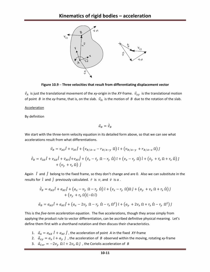
Figure 10.9 ─ Three velocities that result from differentiating displacement vector

�⃗�𝐴 is just the translational movement of the xy-origin in the XY-frame. �⃗�𝑥𝑦 is the translational motion

of point B in the xy-frame, that is, on the slab. �⃗�Ω is the motion of B due to the rotation of the slab.

Acceleration

By definition

�⃗�𝐵 = �̇⃗�𝐵

We start with the three-term velocity equation in its detailed form above, so that we can see what

accelerations result from what differentiations.

�⃗�𝐵 = 𝑣𝐴𝑋𝐼 + 𝑣𝐴𝑌𝐽 + (𝑣𝐵 𝐴⁄ −𝑥 − 𝑟𝐵 𝐴⁄ −𝑦 Ω) 𝑖̂ + (𝑣𝐵 𝐴⁄ −𝑦 + 𝑟𝐵 𝐴⁄ −𝑥 Ω) 𝑗̂

�̇⃗�𝐵 = �̇�𝐴𝑋𝐼 + 𝑣𝐴𝑋𝐼̇ + �̇�𝐴𝑌𝐽+𝑣𝐴𝑌𝐽̇ + (�̇�𝑥 − �̇�𝑦 Ω − 𝑟𝑦 Ω̇) 𝑖̂ + (𝑣𝑥 − 𝑟𝑦 Ω) 𝑖̂̇ + (�̇�𝑦 + �̇�𝑥 Ω + 𝑟𝑥 Ω̇) 𝑗̂

+ (𝑣𝑦 + 𝑟𝑥 Ω) 𝑗̂̇

Again 𝐼 and 𝐽 belong to the fixed frame, so they don’t change and are 0. Also we can substitute in the

results for 𝑖̂ ̇ and 𝑗̂̇ previously calculated. �̇� is 𝑣, and �̇� is 𝑎 .

�̇⃗�𝐵 = 𝑎𝐴𝑋𝐼 + 𝑎𝐴𝑌𝐽 + (𝑎𝑥 − 𝑣𝑦 Ω − 𝑟𝑦 Ω̇) 𝑖̂ + (𝑣𝑥 − 𝑟𝑦 Ω)Ω 𝑗̂ + (𝑎𝑦 + 𝑣𝑥 Ω + 𝑟𝑥 Ω̇) 𝑗̂

+ (𝑣𝑦 + 𝑟𝑥 Ω)(−Ω 𝑖)̂

�⃗�𝐵 = 𝑎𝐴𝑋𝐼 + 𝑎𝐴𝑌𝐽 + (𝑎𝑥 − 2𝑣𝑦 Ω − 𝑟𝑦 Ω̇ − 𝑟𝑥 Ω2) 𝑖̂ + (𝑎𝑦 + 2𝑣𝑥 Ω + 𝑟𝑥 Ω̇ − 𝑟𝑦 Ω2) 𝑗 ̂

This is the five-term acceleration equation. The five accelerations, though they arose simply from

applying the product rule to vector differentiation, can be ascribed definitive physical meaning. Let’s

define them first with a shorthand notation and then discuss their characteristics.

1. �⃗�𝐴 = 𝑎𝐴𝑋 𝐼 + 𝑎𝐴𝑌 𝐽 , the acceleration of point A in the fixed XY-frame

2. �⃗�𝑥𝑦 = 𝑎𝑥 𝑖̂ + 𝑎𝑦 𝑗̂ , the acceleration of B observed within the moving, rotating xy-frame

3. �⃗�𝐶𝑜𝑟 = −2𝑣𝑦 Ω 𝑖̂ + 2𝑣𝑥 Ω 𝑗 ̂ , the Coriolis acceleration of B


10-12

4. �⃗�𝑡 = −𝑟𝑦 Ω̇ 𝑖̂ + 𝑟𝑥 Ω̇ 𝑗̂ , the tangential acceleration of B

5. �⃗�𝑛 = −𝑟𝑥 Ω2 𝑖̂ − 𝑟𝑦 Ω2 𝑗̂ , the normal acceleration of B

So

�⃗�𝐵 = �⃗�𝐴 + �⃗�𝑥𝑦 + �⃗�𝐶𝑜𝑟 + �⃗�𝑡 + �⃗�𝑛

�⃗�𝐴 and �⃗�𝑥𝑦 are both independent accelerations and do not involve the rotation of the slab. Normally

in an analysis they will have to be given or observed. The other three accelerations do involve the

rotation of the slab. �⃗�𝑡 involves a speed-up of the tangential velocity, �⃗�Ω , simply because the spin

speed is increasing…or a slow-down in �⃗�Ω because the spin speed is decreasing. �⃗�𝑛 is due to the

constant change in direction of �⃗�Ω as it seemingly rotates about A . Note that this is directed opposite

to 𝑟𝑥𝑦 , which is 𝑟𝐵/𝐴 . The third term, Coriolis acceleration, is the most puzzling and misunderstood of

the five. It results from a combination of movements: movement on the slab while it is rotating. It was

not even known until long after Newton developed his three laws and Euler extended them to rigid

bodies.

The three accelerations involving Ω⃗⃗⃗ can also be cast as cross products.

3. �⃗�𝐶𝑜𝑟 = 2 Ω⃗⃗⃗ × �⃗�𝑥𝑦 , the Coriolis acceleration of B

4. �⃗�𝑡 = Ω⃗⃗⃗̇× 𝑟𝑥𝑦 , the tangential acceleration of B

5. �⃗�𝑛 = Ω⃗⃗⃗ × (Ω⃗⃗⃗ × 𝑟𝑥𝑦) , the normal acceleration of B

That these are equivalent to the unit-vector versions above can be seen as follows. The magnitude

equivalency can be verified by inspection. The directions can be seen in that in 2-D, positive Ω⃗⃗⃗ and Ω̇⃗⃗⃗

point out of the slab. Using them as the first vector in a cross product produces a vector that is rotated

90° to the right of the second vector in the cross-product. Also, since both Ω⃗⃗⃗ and Ω̇⃗⃗⃗ point in the �̂�

direction (if they are positive), they will convert 𝑖-̂components into 𝑗̂-components and 𝑗̂-components

into −𝑖-̂components. Note that �⃗�𝐶𝑜𝑟 and �⃗�𝑡 have y-components in the −𝑖-̂direction and x-

components in the 𝑗̂-direction. With �⃗�𝑛 , Ω⃗⃗⃗ is used twice as the first vector in a cross product. Thus

the direction is turned 180° around from 𝑟𝑥𝑦 . In the second pre-cross, the x-components that had been

turned into the 𝑗̂-direction get turned another 90° into the −𝑖-̂direction. Note that in the unit-vector

version of �⃗�𝑛 , x-components stay as 𝑖-̂components, and y-components stay as 𝑗̂-components…but

both are now negative.


10-13

Figure 10.10 ─ Five accelerations with a rotating frame

<In drawing above change aC to aCor.>

The figure above shows an example of the five accelerations. �⃗�𝐴 and �⃗�𝑥𝑦 are independent and could

be drawn in any direction. The Coriolis acceleration is perpendicular and to the left of �⃗�𝑥𝑦 since the

slab is rotating counter-clockwise. �⃗�𝑡 is perpendicular and to the left of the line from A to B since Ω̇⃗⃗⃗

is counter-clockwise. �⃗�𝑛 leads from B back toward the apparent center of rotation at A .

Though this is explained in 2-D for visualization purposed, it is equally valid for 3-D.

Also noteworthy is that the center of rotation of the slab does not have to be at A . It does look to an

observer at A as if the slab is rotating about him. But the rotation point does not even have to be fixed.

It could change with time, like an instant center does, in the general case. It could even be, if we take

the special case of B not moving on the slab, that B is the center of rotation. But all of the above is

still true, and we can center our rotating coordinate system at any point on the slab. I would like to

work out this counter-case at some point, just to demonstrate it.

Relationship between large- and small-letter coordinate systems

In the three-term velocity equation and in the five-term acceleration equation, the first term on the

right will be in the large-letter coordinate system and the rest in the small-letter coordinate system. It

will be desired to get everything in the large-letter system, so expressions need to be worked out for 𝑖 ̂,

𝑗̂ , and �̂� in terms of 𝐼 , 𝐽 , and �̂� . We return to the original drawing, which explained the scenario,

and focus on the two sets of unit vectors.


10-14

Figure 10.11 ─ Relationship between small- and large-letter unit vectors

Referring to the magnified drawing of the unit vectors at right, we can see that

𝑖̂ = cos 𝜃 𝐼 + sin 𝜃 𝐽

𝑗̂ = −sin 𝜃 𝐼 + cos 𝜃 𝐽

The last four terms of the acceleration are written in terms of 𝑖 ̂ and 𝑗̂ . They will have to have these

expressions substituted in to have these acceleration in the fixed coordinate system.

It is also possible to convert everything into the small-letter system. Newton’s Second Law applies only

to an inertial (big-letter) coordinate system. But it can be applied there and then the equation

converted to the non-inertial (small-letter) coordinate system by simple coordinate transformations.

The equation transformed into the small-letter system does not lose its validity. What is not valid is

applying Newton’s Second Law with reference to a non-inertial system. This is a subtle but critical point.

10.4 Coriolis acceleration

By derivation of the five-term acceleration equation with a spinning and translating reference frame, we

see that there are two terms that appear when an object moves inside this rotating frame. One of these

is Coriolis acceleration, which was not well known until long after Newton worked out his three laws and

Euler applied them to rigid bodies. The Coriolis term is

�⃗�𝐶𝑜𝑟 = 2Ω⃗⃗⃗ × �⃗�𝑥𝑦

How this term arises mathematically when there is movement in a rotating frame is covered in the

previous section. This section explains Coriolis acceleration from a more pragmatic standpoint, to allow

you to develop your intuition a bit regarding this non-intuitive concept.

First note that the components of Coriolis acceleration involve only two velocities: 1) the rotational

velocity of the rotating frame, usually attached to a rotating body, and 2) the velocity of an object within

this rotating frame. A simple case would be a rotating rod with a collar moving along the rod as shown


10-15

in the figure below. Thus, like normal acceleration, Coriolis acceleration results from velocity. But

unlike conventional acceleration, it is not the time derivative of velocity but rather results from a

combination of velocities.

Figure 10.12 ─ Rotating rod with sliding collar

To explain Coriolis and give some examples of how it manifests itself, I’d like to avail myself of a scenario

that was used to explain Coriolis to me, when I was studying engineering at Mississippi State University

in the middle 1970s. This is a cockroach walking on a vinyl LP record as shown in the figure below.

Figure 10.13 ─ Cockroach walking out on a rotating LP platter

Let’s consider the simple situation where the rotational speed is constant and the cockroach’s

walking velocity is also constant. Obviously as the cockroach walks outward, his distance from the

center of rotation increases, and therefore his velocity due to the rotation increases. Let’s look at this in

detail.

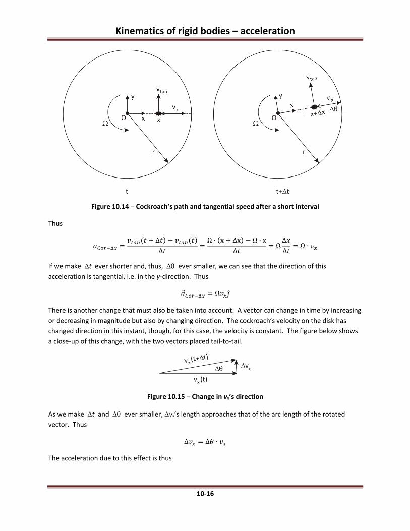
The figure below shows the cockroach at an instant in time ( t ) and then at another instant shortly

thereafter ( t+t ). The disk has turned through a small angle , and the cockroach has moved out a

tiny amount x. At t the tangential velocity v is · x At t+t , because of the increased radius, the

tangential velocity vtan has increased to · (x+x) This increase in vtan is part of the Coriolis

acceleration.


10-16

Figure 10.14 ─ Cockroach’s path and tangential speed after a short interval

Thus

𝑎𝐶𝑜𝑟−∆𝑥 =𝑣𝑡𝑎𝑛(𝑡 + ∆𝑡) − 𝑣𝑡𝑎𝑛(𝑡)

∆𝑡=

Ω ∙ (x + ∆x) − Ω ∙ x

∆𝑡= Ω

∆𝑥

∆𝑡= Ω ∙ 𝑣𝑥

If we make t ever shorter and, thus, ever smaller, we can see that the direction of this

acceleration is tangential, i.e. in the y-direction. Thus

�⃗�𝐶𝑜𝑟−∆𝑥 = Ω𝑣𝑥𝑗 ̂

There is another change that must also be taken into account. A vector can change in time by increasing

or decreasing in magnitude but also by changing direction. The cockroach’s velocity on the disk has

changed direction in this instant, though, for this case, the velocity is constant. The figure below shows

a close-up of this change, with the two vectors placed tail-to-tail.

Figure 10.15 ─ Change in vx’s direction

As we make t and ever smaller, vx’s length approaches that of the arc length of the rotated

vector. Thus

∆𝑣𝑥 = ∆𝜃 ∙ 𝑣𝑥

The acceleration due to this effect is thus


10-17

𝑎𝐶𝑜𝑟−∆𝜃 =∆𝑣𝑥

∆𝑡=

∆𝜃 ∙ 𝑣𝑥

∆𝑡= Ω ∙ 𝑣𝑥

exactly the same result as before, due to the increase in tangential velocity. It is also easy to see that

with a very small , the direction of this acceleration is exactly the same as that of �⃗�𝐶𝑜𝑟−∆𝑥 , that is in

the y-direction. Thus

�⃗�𝐶𝑜𝑟−∆𝜃 = Ω𝑣𝑥𝑗 ̂

The total Coriolis acceleration is thus the combination of these two effects.

�⃗�𝐶𝑜𝑟 = �⃗�𝐶𝑜𝑟−∆𝑥 + �⃗�𝐶𝑜𝑟−∆𝜃 = 2Ω𝑣𝑥𝑗 ̂

Note that this is precisely the same as the cross product that results from deriving the five-term

acceleration equation.

�⃗�𝐶𝑜𝑟 = 2Ω⃗⃗⃗ × �⃗�𝑥𝑦

This equation is more general because we are not constraining the cockroach just to walk on a straight

path along the x-axis. The same type of analysis could be done for any random path with the same

result.

One thing interesting about Coriolis acceleration that is shown by the cross product is this: If the disk is

rotating counter-clockwise, so that Ω⃗⃗⃗ = Ω�̂� , the Coriolis acceleration is always directed to the left of

the path taken by the cockroach. With clockwise rotation, Coriolis acceleration is 90° to the right of the

path.

Some interesting cases

Figure 10.16 ─ Cockroach walking on circular path in direction of rotation

At left the cockroach has turned and is walking in a circular path around the platter. With this, his tangential speed

will increase by vxy from what it would be due to alone. That is

𝑣𝑡𝑎𝑛 = Ω𝑟𝑝 + 𝑣𝑥𝑦

If a light were put on the bug’s back and the lights were turned out, one would simply see the cockroach circling a central point with a tangential speed vtan . His absolute

rotational velocity would be Ω𝑋𝑌 =𝑣𝑡𝑎𝑛

𝑟𝑝. As can be seen,

�⃗�𝑛 and �⃗�𝐶𝑜𝑟 are aligned and point from the cockroach toward point O . These, then, added together, should produce the normal acceleration that one would get using Ω𝑋𝑌 instead to calculate it.


10-18

That is,

�⃗�𝑛 + �⃗�𝐶𝑜𝑟 = Ω2𝑟𝑝 + 2Ω𝑣𝑥𝑦

But just considering the motion of the bug alone

�⃗�𝑛−𝑋𝑌 = Ω𝑋𝑌2 𝑟𝑝 = (

𝑣𝑡𝑎𝑛

𝑟𝑝)

2

𝑟𝑝 =(Ω𝑟𝑝 + 𝑣𝑥𝑦)

2

𝑟𝑝= Ω2𝑟𝑝 + 2Ω𝑣𝑥𝑦 +

𝑣𝑥𝑦2

𝑟𝑝

Thus, it looks as if there is a discrepancy between the two calculations, since the latter one includes the

extra term 𝑣𝑥𝑦2 /𝑟𝑝 . Where does this term come from? The answer is found by considering what the

bug’s acceleration would be, walking on his circular path when = 0 . His normal acceleration on a non-

spinning disk would be precisely 𝑣𝑥𝑦2 /𝑟𝑝 . Thus �⃗�𝑛 + �⃗�𝐶 does not include the local acceleration, �⃗�𝑥𝑦 =

𝑣𝑥𝑦2 /𝑟𝑝 due simply to the cockroach’s walking a circular path. That too needs to be included, so this

latter analysis with the three accelerations is correct, not the former analysis that ignores the 𝑣𝑥𝑦2 /𝑟𝑝

term. A lesson here: when analyzing acceleration with a rotating frame, one must return religiously to

the five-term acceleration equation and rigorously review and include all terms that do not fall out.

Another interesting variant of this case is if the cockroach turned around and walked against the

direction of rotation at a speed that stop his motion, so that 𝑣𝑡𝑎𝑛 = 0; he is simply marching along in

place with the disk is turning under him. If a light were place on his back and the lights turned off, that

light would not move. Now the interesting question is, is he experiencing any acceleration? Do the legs

on both sides of his body feel the same effort when he walks?

Here

𝑣𝑥𝑦 = −Ω𝑟𝑝

If we apply that to the three-term equation above,

�⃗�𝑛−𝑋𝑌 = Ω2𝑟𝑝 + 2Ω𝑣𝑥𝑦 +𝑣𝑥𝑦

2

𝑟𝑝= Ω2𝑟𝑝 − 2Ω2𝑟𝑝 +

(−Ω𝑟𝑝)2

𝑟𝑝= 0

So the answer is that he marches along, feeling no extra push on the legs on either side of his body. If

we back up and look at this globally, the cockroach is stationary in space, in the XY system. With no

motion, specifically no acceleration, he feels no effort on his legs at all. In fact, were he to stop on the

rotating disk, he would feel pressure on his outside legs just standing there, to allow him to travel on the

circular path caused by .


10-19

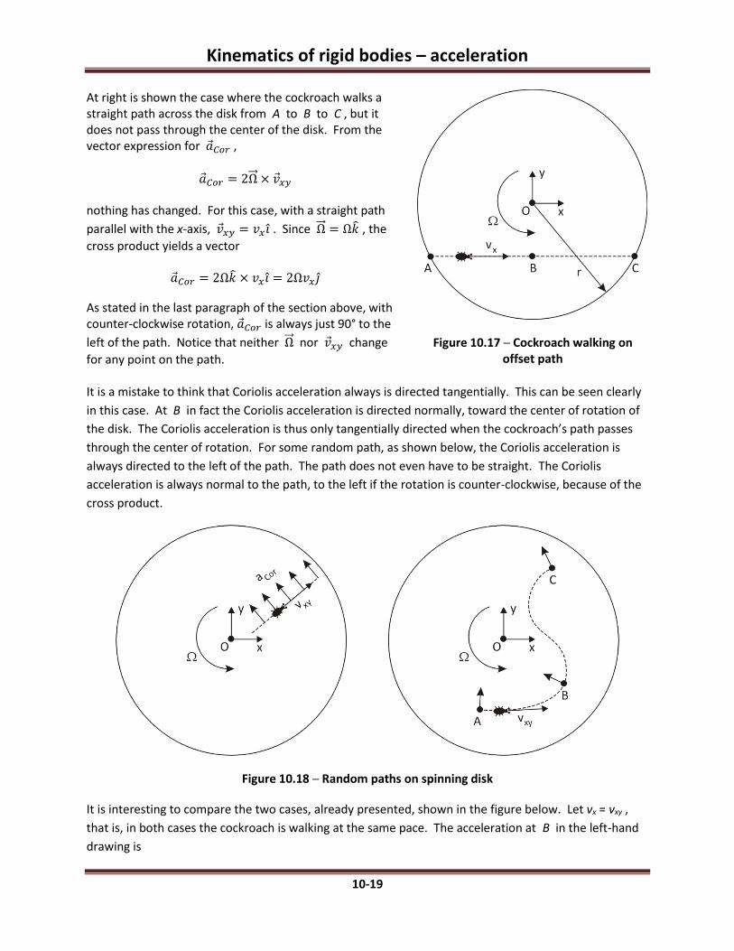
At right is shown the case where the cockroach walks a straight path across the disk from A to B to C , but it does not pass through the center of the disk. From the vector expression for �⃗�𝐶𝑜𝑟 ,

�⃗�𝐶𝑜𝑟 = 2Ω⃗⃗⃗ × �⃗�𝑥𝑦

nothing has changed. For this case, with a straight path

parallel with the x-axis, �⃗�𝑥𝑦 = 𝑣𝑥 �̂� . Since Ω⃗⃗⃗ = Ω�̂� , the

cross product yields a vector

�⃗�𝐶𝑜𝑟 = 2Ω�̂� × 𝑣𝑥 �̂� = 2Ω𝑣𝑥𝑗 ̂

As stated in the last paragraph of the section above, with counter-clockwise rotation, �⃗�𝐶𝑜𝑟 is always just 90° to the

left of the path. Notice that neither Ω⃗⃗⃗ nor �⃗�𝑥𝑦 change

for any point on the path.

Figure 10.17 ─ Cockroach walking on offset path

It is a mistake to think that Coriolis acceleration always is directed tangentially. This can be seen clearly

in this case. At B in fact the Coriolis acceleration is directed normally, toward the center of rotation of

the disk. The Coriolis acceleration is thus only tangentially directed when the cockroach’s path passes

through the center of rotation. For some random path, as shown below, the Coriolis acceleration is

always directed to the left of the path. The path does not even have to be straight. The Coriolis

acceleration is always normal to the path, to the left if the rotation is counter-clockwise, because of the

cross product.

Figure 10.18 ─ Random paths on spinning disk

It is interesting to compare the two cases, already presented, shown in the figure below. Let vx = vxy ,

that is, in both cases the cockroach is walking at the same pace. The acceleration at B in the left-hand

drawing is


10-20

�⃗�𝑛 + �⃗�𝐶𝑜𝑟 = Ω2𝑟𝑝 + 2Ω𝑣𝑥𝑦

Figure 10.19 ─ Comparison of accelerations on a straight path and a circular path

The acceleration in the right-hand drawing is instead

�⃗�𝑛 + �⃗�𝐶𝑜𝑟 + �⃗�𝑥𝑦 = Ω2𝑟𝑝 + 2Ω𝑣𝑥𝑦 +𝑣𝑥𝑦

2

𝑟𝑝

What’s interesting about this is that at B , the tangential velocity of the cockroach in both cases is the

same. But the difference between the two can be seen in the case of a non-spinning disk. Even with no

rotation, the cockroach on the right-hand disk experiences an acceleration toward point O , because of

his circular path. The cockroach on the left-hand disk, on the other hand, would experience no

acceleration, were = 0. Said another way, if the disk is not spinning, the cockroach walking the

straight path feels equal effort in the legs on each side of his body. But the cockroach walking the

circular path must push a little bit harder with his outside legs to turn himself around the center point

that he is circling.

kinematics of rigid bodies – accelerationfowen/me212/10rigidbodykinematicsacceleration.pdfthat...

Documents