kinematic wave technique applied to hydrologic distributed...

Hydrology Days 2008

Kinematic wave technique applied to hydrologic distributed modeling using stationary storm events: an application to synthetic rectangular basins and an actual watershed Michael J. Shultz1 National Weather Service – West Gulf River Forecast Center, Fort Worth, Texas Ernest C. Crosby2

TranSystems, Fort Worth, Texas John A. McEnery3

Department of Civil Engineering, University of Texas at Arlington, Arlington, Texas Abstract. The purpose of this investigation was to evaluate the use of the kinematic wave technique as applied to hydrologic distributed modeling. Distributed models were developed for several artificial rectangular basins and an actual drainage basin using the U.S. Geological Survey Modular Modeling System. Distributed rainfall was applied to the selected basins in the form of stationary storm events. Impervious watershed conditions were assumed for each simulation. The kinematic wave technique was used to route both overland and channel flow. The distributed rainfall was applied as three individual cases over equal areas of the upper, middle, and lower sections of both the synthetic rectangular basins and the actual drainage basin (Cowleech Fork Sabine River near Greenville, Texas). Hydrologic simulations were conducted for each case and the hydrologic responses, as identified by peak flow and overall shape of the hydrographs at the basin outlets, were compared. Both peak flow and hydrograph shapes were similar. No appreciable hydrograph attenuation occurred. Distributed modeling has great potential for the advancement of the hydrologic sciences. Knowledge gained from this investigation may be useful in determining the practical applicability of the kinematic wave technique for use in distributed models. 1. Introduction

Distributed models have great potential to advance the hydrologic sciences by improving the accuracy of hydrologic simulations. Distributed models utilize high resolution data which takes into account the spatial variability of both the physiographic characteristics of a drainage area and the meteorological factors such as precipitation. Because of this, they are often perceived as more accurate than the traditional lumped model, which represents a whole hydrologic unit based on uniformity of rainfall and hydrologic parameters across the basin.

1 National Weather Service, West Gulf River Forecast Center, 3401 Northern Cross Blvd., Fort Worth, TX 76137; Tel: (817) 831-3289, ext. 218; e-mail: [email protected] 2 TranSystems, 500 W. 7th Street, Suite 1100, Fort Worth, TX 76102; Tel: (817) 334-4422; e-mail: [email protected] 3 University of Texas at Arlington, Department of Civil Engineering, 405 Nedderman Hall, Arlington, TX 76019; Tel: (817) 272-0234; e-mail: [email protected]

Kinematic wave approach for distributed hydrologic modeling

117

Distributed models quite often employ the kinematic wave routing technique to simulate both overland and channel flow. The kinematic wave has provided a solid foundation for the development of this science. However, the kinematic wave has limitations which may hinder its application within distributed models. 2. Kinematic Wave Technique The kinematic wave technique is a simplified version of the dynamic wave technique. The full dynamic wave takes into account the entire spectrum of the physical processes which simulate hydrologic flow along a stream channel. The kinematic wave simplifies these processes by assuming various physical processes as negligible.

Dynamic wave models are based on one-dimensional gradually varied unsteady open channel flow. The dynamic wave consists of two partial differential equations (continuity and momentum), otherwise referred to as the Saint-Venant equations. The Saint-Venant equations take into account the physical laws which govern both conservation of mass (continuity) and conservation of momentum (dynamic). These physical factors consist of local acceleration, convective acceleration, hydrostatic pressure forces, gravitational forces, and frictional forces.

Kinematic wave models are based on the continuity equation and a simplified form of the momentum equation used for the full dynamic wave. The physical factors which govern the kinematic wave are gravitational forces and frictional forces (Fread, 1988; Chow, 1988; HEC, 1990; COE, 1991; Mays, 1996; Maidment, 1993). 2.1. Continuity Equation

The continuity equation applies to both dynamic waves and kinematic waves. The equation is based on the principle of the conservation of mass and is written as

where Q is the discharge (cfs), A is the cross-sectional area (sq ft), q is the lateral inflow per unit length (cfs per ft), x is the space coordinate (ft), and t is the time (seconds) (Chow, 1988; Mays, 1996; Shultz, 1992). 2.2. Momentum Equation (Dynamic Wave Form)

The momentum equation applies to the full dynamic wave. The equation is based on Newton’s second law of motion and is written as

Shultz et al.

118

where y is the flow depth, V is the mean velocity, g is the gravitational acceleration, So is the bed slope, and Sf is the friction slope (Chow 1988; Mays, 1996; Singh, 1996; Shultz, 1992). 2.3. Momentum Equation (Kinematic Wave Form)

The simplified version of the full dynamic wave equation applies to kinematic waves. This equation is

where Sf is the friction slope and So is the bed slope (gravity) (Singh, 1996; Chow, 1988; Mays, 1996; Shultz, 1992). 2.4. Comparison of the Kinematic and Dynamic Wave Techniques The dynamic wave equations govern the movement of a flood wave traversing downstream in a channel taking into account gravity, friction, inertia (acceleration), and pressure. The kinematic wave considers only gravity and friction, assuming inertia (acceleration) and pressure as negligible. The weight component (gravity) is balanced by the resistive forces (channel bed friction), allowing little to no acceleration of the floodwave. This results in uniform flow. By neglecting pressure and inertia, the primary mechanism which causes the flood wave to attenuate is eliminated. Any indication of attenuation is through numerical error associated with the finite-difference scheme, not the physical mechanisms associated with the actual movement of a flood wave. Because of this, there may be limitations to the use of the kinematic wave for distributed model applications (HEC, 1990; Maidment, 1993; Mays, 1996; Overton, 1976; Shultz, 1992, 2007). 3. Modular Modeling System (MMS) The USGS Modular Modeling System (MMS) is a modeling framework used to develop, support, and apply dynamic models to water resource applications. MMS was used in this study to develop distributed models using the kinematic wave technique (Alley, 1982; Leavesley, 1983, 2004). Within MMS is the Precipitation-Runoff Modeling System (PRMS) module. PRMS is used to simulate the hydrologic response of a drainage basin due to rainfall over various combinations of land use and watershed conditions. Within PRMS, each component of the hydrologic cycle is expressed in terms of known physical laws or empirical relationships. These laws and relationships have some physical interpretation based on measurable characteristics over watershed basins. This reproduces the physical reality of the hydrologic system to actual watershed conditions as closely as possible. PRMS was used to develop distributed models using the kinematic wave technique. Drainage basins are partitioned into units based on watershed characteristics such as slope,


119

aspect, vegetation type, soil type, and precipitation distribution. Hydrologic simulations are then performed based on distributed parameters. 4. Methodology The MMS was used to simulate the hydrologic response which resulted from a stationary rainfall event applied to various locations over the synthetic rectangular drainage basins. Next, the MMS was used to simulate the hydrologic response with the same basic stationary rainfall patterns over a real basin (Cowleech Fork Sabine River near Greenville, Texas). Physical processes which govern the hydrologic response over drainage basins are highly complex. To simplify the problem and better isolate the mechanisms of interest, hydrologic parameters were manually set in order to reflect impervious watershed basins. By isolating these parameters, a better understanding could be gained on the impact the kinematic wave technique has on distributed models using stationary storm events (Shultz, 2007). 4.1 Synthetic Rectangular Drainage Basins

The synthetic rectangular drainage basins used for this part of the study were bisected in half lengthwise by a major drainage channel forming two symmetrical overland flow planes. The length of the basin was then subdivided into 10 sections, creating a total of 20 overland flow planes. The rectangular dimensions for each basin were based on typical watershed shape factors of 1, 2, 3, 4, and 5. Shape factor is the length to width ratio of a drainage basin. As the shape factor increases, the basin becomes longer and narrower. The configurations for these basins are shown with the results in Section 5.1. Physiographic characteristics of the watershed were selected which are typical of conditions found over the State of Texas. Three overland flow plane slopes (i.e. 16.22%, 9.12%, and 4.05%) along with a channel slope of 1.55% were selected for each basin. A Manning’s n roughness coefficient of 0.15 was selected for the overland flow plane. This represents tall grass vegetation. Also, a Manning’s n roughness coefficient of 0.05 was selected for the channel (FHA, 2001).

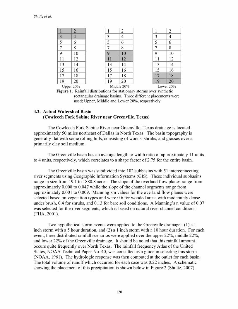
Three hypothetical distributed rainfall scenarios consisting of a 1 inch amount over a 10 minute time period were placed over the upper 20%, middle 20%, and lower 20% of each synthetic rectangular basin. This is approximately equal to a 2 year-10 minute storm intensity frequency for North Texas, outlined in NOAA Technical Memorandum NWS HYDRO-35 (NOAA 1977). The hydrologic response was then computed at the outlet for each basin. The total volume of runoff which occurred for each case was 0.2 inches. A schematic showing the placement of this precipitation is shown below in Figure 1 (Shultz 2007).

Shultz et al.

120

1 2 1 2 1 2 3 4 3 4 3 4 5 6 5 6 5 6 7 8 7 8 7 8 9 10 9 10 9 10 11 12 11 12 11 12 13 14 13 14 13 14 15 16 15 16 15 16 17 18 17 18 17 18 19 20 19 20 19 20

Upper 20% Middle 20% Lower 20% Figure 1. Rainfall distributions for stationary storms over synthetic

rectangular drainage basins. Three different placements were used; Upper, Middle and Lower 20%, respectively.

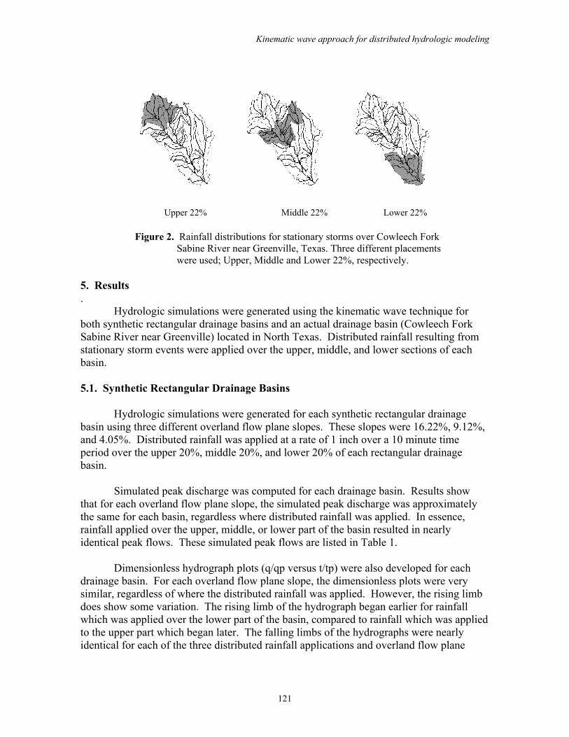
4.2. Actual Watershed Basin (Cowleech Fork Sabine River near Greenville, Texas) The Cowleech Fork Sabine River near Greenville, Texas drainage is located approximately 50 miles northeast of Dallas in North Texas. The basin topography is generally flat with some rolling hills, consisting of woods, shrubs, and grasses over a primarily clay soil medium. The Greenville basin has an average length to width ratio of approximately 11 units to 4 units, respectively, which correlates to a shape factor of 2.75 for the entire basin. The Greenville basin was subdivided into 102 subbasins with 51 interconnecting river segments using Geographic Information Systems (GIS). These individual subbasins range in size from 19.1 to 1880.8 acres. The slope of the overland flow planes range from approximately 0.008 to 0.047 while the slope of the channel segments range from approximately 0.001 to 0.009. Manning’s n values for the overland flow planes were selected based on vegetation types and were 0.6 for wooded areas with moderately dense under brush, 0.4 for shrubs, and 0.13 for bare soil conditions. A Manning’s n value of 0.07 was selected for the river segments, which is based on natural river channel conditions (FHA, 2001). Two hypothetical storm events were applied to the Greenville drainage: (1) a 1 inch storm with a 5 hour duration, and (2) a 1 inch storm with a 10 hour duration. For each event, three distributed rainfall scenarios were applied over the upper 22%, middle 22%, and lower 22% of the Greenville drainage. It should be noted that this rainfall amount occurs quite frequently over North Texas. The rainfall frequency Atlas of the United States, NOAA Technical Paper No. 40, was consulted as a guide in selecting this storm (NOAA, 1961). The hydrologic response was then computed at the outlet for each basin. The total volume of runoff which occurred for each case was 0.22 inches. A schematic showing the placement of this precipitation is shown below in Figure 2 (Shultz, 2007).


121

Upper 22% Middle 22% Lower 22%

Figure 2. Rainfall distributions for stationary storms over Cowleech Fork

Sabine River near Greenville, Texas. Three different placements were used; Upper, Middle and Lower 22%, respectively.

5. Results .

Hydrologic simulations were generated using the kinematic wave technique for both synthetic rectangular drainage basins and an actual drainage basin (Cowleech Fork Sabine River near Greenville) located in North Texas. Distributed rainfall resulting from stationary storm events were applied over the upper, middle, and lower sections of each basin. 5.1. Synthetic Rectangular Drainage Basins Hydrologic simulations were generated for each synthetic rectangular drainage basin using three different overland flow plane slopes. These slopes were 16.22%, 9.12%, and 4.05%. Distributed rainfall was applied at a rate of 1 inch over a 10 minute time period over the upper 20%, middle 20%, and lower 20% of each rectangular drainage basin.

Simulated peak discharge was computed for each drainage basin. Results show that for each overland flow plane slope, the simulated peak discharge was approximately the same for each basin, regardless where distributed rainfall was applied. In essence, rainfall applied over the upper, middle, or lower part of the basin resulted in nearly identical peak flows. These simulated peak flows are listed in Table 1.

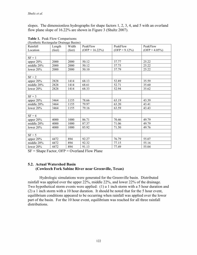
Dimensionless hydrograph plots (q/qp versus t/tp) were also developed for each

drainage basin. For each overland flow plane slope, the dimensionless plots were very similar, regardless of where the distributed rainfall was applied. However, the rising limb does show some variation. The rising limb of the hydrograph began earlier for rainfall which was applied over the lower part of the basin, compared to rainfall which was applied to the upper part which began later. The falling limbs of the hydrographs were nearly identical for each of the three distributed rainfall applications and overland flow plane

Shultz et al.

122

slopes. The dimensionless hydrographs for shape factors 1, 2, 3, 4, and 5 with an overland flow plane slope of 16.22% are shown in Figure 3 (Shultz 2007).

Table 1. Peak Flow Comparisons (Synthetic Rectangular Drainage Basins) Rainfall Location

Length (feet)

Width (feet)

PeakFlow (OFP = 16.22%)



SF = 1 upper 20% 2000 2000 50.12 37.77 25.22 middle 20% 2000 2000 50.12 37.75 25.22 lower 20% 2000 2000 50.10 37.79 25.22 SF = 2 upper 20% 2828 1414 68.13 52.89 35.59 middle 20% 2828 1414 68.61 52.71 35.60 lower 20% 2828 1414 68.33 52.94 35.62 SF = 3 upper 20% 3464 1155 78.66 63.19 43.39 middle 20% 3464 1155 79.97 63.20 43.41 lower 20% 3464 1155 79.16 63.59 43.43 SF = 4 upper 20% 4000 1000 86.71 70.46 49.79 middle 20% 4000 1000 87.37 71.06 49.79 lower 20% 4000 1000 85.92 71.50 49.76 SF = 5 upper 20% 4472 894 92.27 76.79 55.07 middle 20% 4472 894 92.32 77.15 55.16 lower 20% 4472 894 91.13 77.49 55.04 SF = Shape Factor, OFP = Overland Flow Plane 5.2. Actual Watershed Basin (Cowleech Fork Sabine River near Greenville, Texas)

Hydrologic simulations were generated for the Greenville basin. Distributed rainfall was applied over the upper 22%, middle 22%, and lower 22% of the drainage. Two hypothetical storm events were applied: (1) a 1 inch storm with a 5 hour duration and (2) a 1 inch storm with a 10 hour duration. It should be noted that for the 5 hour event, equilibrium conditions appeared to be occurring when rainfall was applied over the lower part of the basin. For the 10 hour event, equilibrium was reached for all three rainfall distributions.


123

Shape Factor = 1 Shape Factor = 2

Shape Factor = 3 Shape Factor = 4

Shape Factor = 5

Figure 3. Dimensionless hydrographs for stationary storms over synthetic rectangular drainage basins with an overland flow plane slope of 16.22%. Note the rising limb of the hydrographs began earlier when the rainfall was applied over the lower part of the basin, while the falling limbs were nearly identical for all distributed rainfall applications.

For both the 5 hour and 10 hour storm durations, simulated peak discharges were computed for the Greenville drainage basin. Results show that for each rainfall event, the simulated peak discharges are similar in magnitude, regardless of where distributed rainfall was applied. Although there are some variations, these differences are relatively small when comparing the three distributed cases. These differences are most likely attributable to the various shapes and drainage configurations of the upper 22%, middle 22%, and lower 22% of the drainage basin. Also, peak discharge is slightly higher for the upper 22% case than for the lower 22%, with the middle 22% lying between these cases. These simulated peak flows are listed in Table 2.

Shultz et al.

124

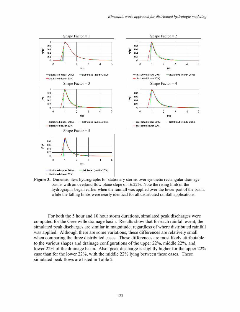
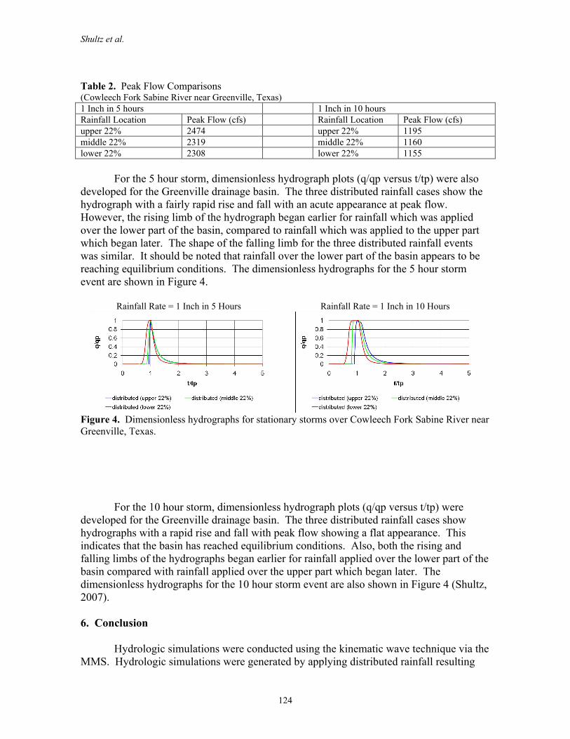
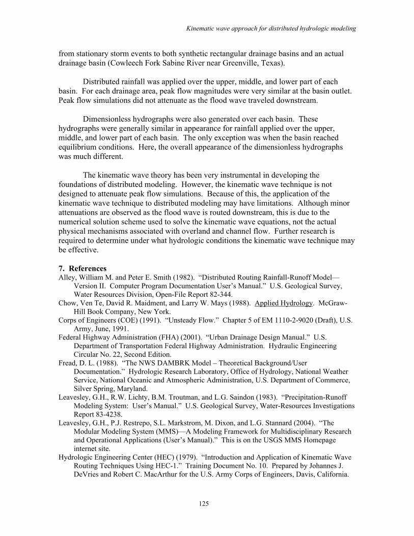
Table 2. Peak Flow Comparisons (Cowleech Fork Sabine River near Greenville, Texas) 1 Inch in 5 hours 1 Inch in 10 hours Rainfall Location Peak Flow (cfs) Rainfall Location Peak Flow (cfs) upper 22% 2474 upper 22% 1195 middle 22% 2319 middle 22% 1160 lower 22% 2308 lower 22% 1155 For the 5 hour storm, dimensionless hydrograph plots (q/qp versus t/tp) were also developed for the Greenville drainage basin. The three distributed rainfall cases show the hydrograph with a fairly rapid rise and fall with an acute appearance at peak flow. However, the rising limb of the hydrograph began earlier for rainfall which was applied over the lower part of the basin, compared to rainfall which was applied to the upper part which began later. The shape of the falling limb for the three distributed rainfall events was similar. It should be noted that rainfall over the lower part of the basin appears to be reaching equilibrium conditions. The dimensionless hydrographs for the 5 hour storm event are shown in Figure 4.

Rainfall Rate = 1 Inch in 5 Hours Rainfall Rate = 1 Inch in 10 Hours

Figure 4. Dimensionless hydrographs for stationary storms over Cowleech Fork Sabine River near Greenville, Texas.

For the 10 hour storm, dimensionless hydrograph plots (q/qp versus t/tp) were developed for the Greenville drainage basin. The three distributed rainfall cases show hydrographs with a rapid rise and fall with peak flow showing a flat appearance. This indicates that the basin has reached equilibrium conditions. Also, both the rising and falling limbs of the hydrographs began earlier for rainfall applied over the lower part of the basin compared with rainfall applied over the upper part which began later. The dimensionless hydrographs for the 10 hour storm event are also shown in Figure 4 (Shultz, 2007). 6. Conclusion Hydrologic simulations were conducted using the kinematic wave technique via the MMS. Hydrologic simulations were generated by applying distributed rainfall resulting


125

from stationary storm events to both synthetic rectangular drainage basins and an actual drainage basin (Cowleech Fork Sabine River near Greenville, Texas). Distributed rainfall was applied over the upper, middle, and lower part of each basin. For each drainage area, peak flow magnitudes were very similar at the basin outlet. Peak flow simulations did not attenuate as the flood wave traveled downstream. Dimensionless hydrographs were also generated over each basin. These hydrographs were generally similar in appearance for rainfall applied over the upper, middle, and lower part of each basin. The only exception was when the basin reached equilibrium conditions. Here, the overall appearance of the dimensionless hydrographs was much different. The kinematic wave theory has been very instrumental in developing the foundations of distributed modeling. However, the kinematic wave technique is not designed to attenuate peak flow simulations. Because of this, the application of the kinematic wave technique to distributed modeling may have limitations. Although minor attenuations are observed as the flood wave is routed downstream, this is due to the numerical solution scheme used to solve the kinematic wave equations, not the actual physical mechanisms associated with overland and channel flow. Further research is required to determine under what hydrologic conditions the kinematic wave technique may be effective. 7. References Alley, William M. and Peter E. Smith (1982). “Distributed Routing Rainfall-Runoff Model—

Version II. Computer Program Documentation User’s Manual.” U.S. Geological Survey, Water Resources Division, Open-File Report 82-344.

Chow, Ven Te, David R. Maidment, and Larry W. Mays (1988). Applied Hydrology. McGraw-Hill Book Company, New York.

Corps of Engineers (COE) (1991). “Unsteady Flow.” Chapter 5 of EM 1110-2-9020 (Draft), U.S. Army, June, 1991.

Federal Highway Administration (FHA) (2001). “Urban Drainage Design Manual.” U.S. Department of Transportation Federal Highway Administration. Hydraulic Engineering Circular No. 22, Second Edition.

Fread, D. L. (1988). “The NWS DAMBRK Model – Theoretical Background/User Documentation.” Hydrologic Research Laboratory, Office of Hydrology, National Weather Service, National Oceanic and Atmospheric Administration, U.S. Department of Commerce, Silver Spring, Maryland.

Leavesley, G.H., R.W. Lichty, B.M. Troutman, and L.G. Saindon (1983). “Precipitation-Runoff Modeling System: User’s Manual.” U.S. Geological Survey, Water-Resources Investigations Report 83-4238.

Leavesley, G.H., P.J. Restrepo, S.L. Markstrom, M. Dixon, and L.G. Stannard (2004). “The Modular Modeling System (MMS)—A Modeling Framework for Multidisciplinary Research and Operational Applications (User’s Manual).” This is on the USGS MMS Homepage internet site.

Hydrologic Engineering Center (HEC) (1979). “Introduction and Application of Kinematic Wave Routing Techniques Using HEC-1.” Training Document No. 10. Prepared by Johannes J. DeVries and Robert C. MacArthur for the U.S. Army Corps of Engineers, Davis, California.

Shultz et al.

126

Hydrologic Engineering Center (HEC) (1990). River Routing With HEC-1 and HEC-2. Training Document No. 30. U.S. Army Corps of Engineers, Davis, California.

Maidment, David R. (1993). Handbook of Hydrology. McGraw-Hill, Inc., New York. Mays, Larry W. (1996). Water Resources Handbook. McGraw-Hill, Inc., New York. National Oceanic and Atmospheric Administration (NOAA) (1961). “Rainfall Frequency Atlas of

the United States for Durations from 30 Minutes to 24 Hours and Return Periods from 1 to 100 years.” U.S. Weather Bureau Technical Paper No. 40.

National Oceanic and Atmospheric Administration (NOAA) (1977). “Five- to 60-Minute Precipitation Frequency for the Eastern and Central United States.” NOAA Technical Memorandum NWS Hydro-35.

Overton, Donald E. and Michael E. Meadows (1976). Stormwater Modeling. Academic Press, New York.

Shultz, Michael J. (1992). Comparison of Flood Routing Methods for a Rapidly Rising Hydrograph Routed Through a Very Wide Channel. Master of Science Thesis, Department of Civil Engineering, College of Engineering, The University of Texas at Arlington.

Shultz, Michael J. (2007). Comparison of Distributed Versus Lumped Hydrologic Simulation Models Using Stationary and Moving Storm Events Applied to Small Synthetic Rectangular Basins and an Actual Watershed Basin. PhD Dissertation, Department of Civil Engineering, College of Engineering, The University of Texas at Arlington.

Singh, Vijay P. (1996). Kinematic Wave Modeling in Water Resources. John Wiley & Sons, Inc., New York

kinematic wave technique applied to hydrologic distributed...

Documents