kinectic energy recovery using compressed gas · variable valve timing (vvt) system that allows the...

University of Southern Queensland

Faculty of Health, Engineering and Sciences

KINETIC ENERGY RECOVERY IN MOTOR VEHICLES USING

COMPRESSED GAS

A dissertation submitted by

Mr. Rick William Kruger

In fulfilment of the requirements of

Bachelor of Engineering (Honours) (Mechanical)

October 2014

i

Abstract

It’s no secret that we are depleting our natural resources at an unsustainable rate while

polluting our natural environment. This is especially true when it comes to motor

vehicles. As a result, manufacturers are investing billions of dollars every year to

produce energy efficient vehicles that reduce fuel consumption and vehicle emissions.

One method is to introduce regenerative braking. This is the process of recovering

kinetic energy from a moving vehicle under braking conditions. The energy is used to

increase performance and efficiency, hence addressing the issues of sustainability and

the environment.

The research of this project was focused on the concept of using an internal combustion

(IC) engine as a compressor to recover kinetic energy as compressed gas. This is a

concept that has been considered over the last decade and a half, with the one of the first

being Schechter (1999). This research project investigates the ability to use the engine

as a compressor and assesses its performance and viability when compared with two

other main regenerative braking technologies: hybrid electric vehicles (HEV) and

flywheels.

A literature review was undertaken, and revealed the major aspects that affect the ability

of an IC engine to compress gas. The major component needed for this concept was a

variable valve timing (VVT) system that allows the engine to operate as a compressor,

and even a pneumatic motor if needed. The system would also require modifications to

the cylinder head to add a charge/discharge valve, and of course, a pressure tank for

storing the compressed gas.

The research methodology considered a quasi-dimensional numerical simulation of an

IC engine operating as a reciprocating two-stroke compressor. The simulation was

based on a model previously prepared by Buttsworth (2002) to determine the

performance of a fuel inducted engine with a heat release profile as a function of the

crank angle – the method that closely followed that described by Ferguson (1986).

ii

After testing, the model was simulated during the deceleration phases of the NEDC test

cycle. The valve timing was optimised to produce the least amount of work during the

simulation, while the engine speed was optimised to reduce the reliance on the friction

brakes. The results showed that the energy recoverable was 574 kJ over the entire cycle

with the assumption that the energy recovered was used after each deceleration event.

Based on an engine efficiency of 30% and usable energy of 80%, this translates to

energy savings of 1.5 MJ and fuel savings of 43 ml over the full cycle.

Overall, the concept of using compressed gas to recover kinetic energy appeared to be

viable. With additional components and modifications, an engine can be used as a

compressor. The advantages seem to be the mass of the system and its simplicity when

compared to HEVs and flywheels. The fuel savings also appear to be competitive.

However, it seems to be less suited for storing energy over longer periods of time, and

has a lower regenerative efficiency as shown in the results of this research and the

research of others. It is unclear whether or not it could compete with HEVs in the

market. The research suggests that more effort needs to be invested in producing

experimental results, and subsequently optimising the system to improve performance.

iii

Acknowledgements

I would like extend thanks to my supervisor Dr Ray Malpress for his ongoing support

and guidance during completion of this dissertation.

I would also like to thank my wife Kahla for her unwavering support throughout this

endeavour and my studies, for her understanding when study commitments meant that

my time was limited, for her infinite patience during the demanding times when mine

was exhausted, and for keeping me focused on the light at end of the tunnel.

iv



ENG4111/ENG4112 Research Project

Limitations of Use

The Council of the University of Southern Queensland, its Faculty of Health,

Engineering & Sciences, and the staff of the University of Southern Queensland, do not

accept any responsibility for the truth, accuracy or completeness of material contained

within or associated with this dissertation.

Persons using all or any part of this material do so at their own risk, and not at the risk

of the Council of the University of Southern Queensland, its Faculty of Health,

Engineering & Sciences or the staff of the University of Southern Queensland.

This dissertation reports an educational exercise and has no purpose or validity beyond

this exercise. The sole purpose of the course pair entitled “Research Project” is to

contribute to the overall education within the student’s chosen degree program. This

document, the associated hardware, software, drawings, and other material set out in the

associated appendices should not be used for any other purpose: if they are so used, it is

entirely at the risk of the user.

v



ENG4111/ENG4112 Research Project

Certification of Dissertation

I certify that the ideas, designs and experimental work, results, analyses and conclusions

set out in this dissertation are entirely my own effort, except where otherwise indicated

and acknowledged.

I further certify that the work is original and has not been previously submitted for

assessment in any other course or institution, except where specifically stated.

Rick William Kruger

Student Number: 0061016558

_____________________

Signature

_____________________

Date

vi

Table of Contents

Abstract .............................................................................................................................. i

Acknowledgements .......................................................................................................... iii

Limitations of Use ............................................................................................................ iv

Certification of Dissertation .............................................................................................. v

List of Figures ................................................................................................................... x

List of Tables.................................................................................................................. xiii

Glossary .......................................................................................................................... xv

1 Introduction ................................................................................................................ 1

Project Background ............................................................................................ 2 1.1

1.1.1 Energy Losses in Passenger Vehicles ..................................................... 3

1.1.2 Kinetic Energy ......................................................................................... 4

1.1.3 Current Technologies .............................................................................. 5

1.1.3.1 Hybrid Electric Vehicles ...................................................................... 5

1.1.3.2 Flywheels ............................................................................................. 9

1.1.4 Conclusion ............................................................................................. 12

Concept ............................................................................................................. 13 1.2

Aims and Objectives ........................................................................................ 14 1.3

Scope ................................................................................................................ 15 1.4

2 Literature Review ..................................................................................................... 16

Internal Combustion Engine as a Compressor ................................................. 16 2.1

2.1.1 Introduction ........................................................................................... 16

2.1.2 Ideal Operating Cycles .......................................................................... 16

2.1.2.1 Ideal Positive Displacement Compressor Cycle ................................ 16

2.1.2.2 Otto Cycle .......................................................................................... 18

2.1.2.3 Operating Analysis ............................................................................ 19

vii

2.1.3 Real Losses ............................................................................................ 20

2.1.3.1 Heat Transfer in Compressors ........................................................... 21

2.1.3.2 Heat Transfer in IC Engines .............................................................. 22

2.1.3.3 Compressor Valve Timing ................................................................. 25

2.1.3.4 IC Engine Valve Timing .................................................................... 25

2.1.3.5 Compressor Flow Losses ................................................................... 27

2.1.3.6 IC Engine Flow Losses ...................................................................... 28

2.1.3.7 Leakage .............................................................................................. 31

2.1.3.8 Mechanical Frictional Losses ............................................................ 32

Applications of Compressed Gas ..................................................................... 33 2.2

2.2.1 Introduction ........................................................................................... 33

2.2.2 Supercharging ........................................................................................ 33

2.2.3 Pneumatic Engines ................................................................................ 36

2.2.3.1 Pneumatic Engine Operation (Hybridized IC Engine) ...................... 36

2.2.3.2 Pneumatic Hybrids ............................................................................. 39

2.2.4 Other Applications ................................................................................ 39

Other Design Factors ........................................................................................ 40 2.3

2.3.1 Air Storage Tank ................................................................................... 40

2.3.1.1 Volume............................................................................................... 40

2.3.1.2 Pressure and Temperature .................................................................. 40

2.3.1.3 Safety ................................................................................................. 42

2.3.2 Cylinder Modifications .......................................................................... 42

2.3.3 Variable Valve Timing .......................................................................... 43

2.3.4 Compression Braking ............................................................................ 44

Conclusion ........................................................................................................ 46 2.4

3 Methodology of the Numerical Simulation ............................................................. 48

Introduction ...................................................................................................... 48 3.1

viii

Model Parameters ............................................................................................. 49 3.2

3.2.1 Operating Assumptions ......................................................................... 49

3.2.2 Modelling Assumptions ........................................................................ 49

3.2.3 Inputs Parameters .................................................................................. 50

3.2.4 Model Losses ......................................................................................... 52

3.2.4.1 Heat Transfer ..................................................................................... 52

3.2.4.2 Flow Losses ....................................................................................... 53

3.2.4.3 Leakage .............................................................................................. 53

Engine Compressor Simulation ........................................................................ 53 3.3

3.3.1 Compression .......................................................................................... 54

3.3.2 Charging ................................................................................................ 54

3.3.3 Air Tank Storage ................................................................................... 55

3.3.4 Expansion .............................................................................................. 56

3.3.5 Intake ..................................................................................................... 57

Model Validation .............................................................................................. 58 3.4

Drive Cycle ....................................................................................................... 63 3.5

4 Results and Discussion ............................................................................................ 67

Introduction ...................................................................................................... 67 4.1

Engine Speed Optimisation .............................................................................. 67 4.2

Energy Recoverable ......................................................................................... 72 4.3

Energy Savings ................................................................................................. 73 4.4

Effect of Losses ................................................................................................ 75 4.5

Other observations ............................................................................................ 76 4.6

4.6.1 Efficiency of Recovery .......................................................................... 76

4.6.2 Pressure and Temperature of the Air Tank Over Time ......................... 78

Limitations ........................................................................................................ 80 4.7

4.7.1 Due to Model Limitations ..................................................................... 80

ix

4.7.2 Due to Assumptions .............................................................................. 81

Conclusion ........................................................................................................ 82 4.8

5 Conclusions .............................................................................................................. 83

Introduction ...................................................................................................... 83 5.1

Viability of the Concept ................................................................................... 83 5.2

5.2.1 Comparison with Current Technologies ................................................ 84

5.2.2 Ability to Use the Engine as a Compressor ........................................... 85

5.2.3 Applications of the Compressed Gas .................................................... 86

Conclusion ........................................................................................................ 86 5.3

Further Work .................................................................................................... 87 5.4

6 References ................................................................................................................ 88

Appendix A – Project Specification ................................................................................ 92

Appendix B1 – Results: Optimised Braking Speed ........................................................ 93

Appendix B2 – Results: Required BMEP vs Actual BMEP ........................................... 94

Appendix B3 – Results: Energy Recovered .................................................................. 100

Appendix C1 – Airdata.m ............................................................................................. 102

Appendix C2 – Compressor_mode.m ........................................................................... 106

Appendix C3 – Enginedata.m ....................................................................................... 112

Appendix C4 – Farg.m .................................................................................................. 113

Appendix C5 – Fueldata.m ........................................................................................... 116

Appendix C6 – Ratescomp.m ....................................................................................... 119

Appendix C7 – Ratesexp.m .......................................................................................... 120

x

List of Figures

Figure 1 – Illustration of the setup of a Hybrid Electric Vehicle (U.S. Government n.d.-

b). ...................................................................................................................................... 6

Figure 2 – Diagram of a flywheel KERS module (Motor Trend Magazine 2014a). ...... 10

Figure 3 – Flywheel KERS system layout (Motor Trend Magazine 2014b). ................. 11

Figure 4 – Ideal compression cycle and pressure-volume diagram of a reciprocating

compressor showing the four processes. Sourced from (Hanlon 2001)......................... 17

Figure 5 – Pressure-volume diagram of the Otto cycle showing the six processes. ....... 18

Figure 6 – Pressure-volume diagram of a compressor with approximate suction and

discharge losses (Hanlon 2001). ..................................................................................... 21

Figure 7 – Typical temperature values found in an SI engine operating at normal steady

state conditions. Temperatures are in degrees C (Pulkrabek 1997). .............................. 23

Figure 8 – Valve-lift curve showing the minimum intake and exhaust flow area as a

function of crank angle (Asmus 1982). ........................................................................... 30

Figure 9 – Idealised pressure-volume diagram of an engine with the option of charging

an air tank during the compression process (Higelin, Charlet & Chamaillard 2002). .... 35

Figure 10 – Ideal pressure-volume diagram of an engine operating as a pneumatic motor

(Schechter 1999). ............................................................................................................ 36

Figure 11 – Pressure-volume diagram of the Air-Power-Assisted cycle for a four-stroke

cycle (Schechter 1999). ................................................................................................... 38

Figure 12 – Pressure-volume diagram of Type 2 compression braking with early charge

valve opening showing a higher IMEP (Schechter 1999). .............................................. 46

Figure 13 – Pressure-volume diagram of Type 2 compression braking with late charge

valve opening showing a higher IMEP (Schechter 1999). .............................................. 46

Figure 14 – Diagram of the processes numerically modelled in MATLAB. .................. 53

Figure 15 – Pressure vs crank angle of the gas in the cylinder for the ideal compression

and expansion processes during testing of the model’s validity. .................................... 58

Figure 16 – Temperature vs crank angle of the gas in the cylinder for the ideal

compression and expansion processes during testing of the model’s validity. ............... 59

xi

Figure 17 – Work performed (for two of the four cylinders) vs crank angle on the gas in

the cylinder for the ideal compression and expansion processes during testing of the

model’s validity. .............................................................................................................. 59

Figure 18 – Pressure of the gas in the cylinder of the ideal compression cycle during

testing of the model validity. ........................................................................................... 60

Figure 19 – Temperature of the gas in the cylinder of the ideal compression cycle during

testing of the model validity. ........................................................................................... 60

Figure 20 – Work performed on the gas in the cylinder of the ideal compression cycle

during testing of the model validity. ............................................................................... 61

Figure 21 – PV diagram of the ideal compression cycle during testing of the model

validity. ........................................................................................................................... 61

Figure 22 – Air tank pressure per engine revolutions compared to the theoretical

maximum pressure for testing the model for validity. .................................................... 62

Figure 23 – Charging valve and intake valve opening timing as a function of crank

angle over time during testing of the model validity. ..................................................... 63

Figure 24 – Graph of speed over time for the Urban Driving Cycle ECE-15 (DieselNet

2013). .............................................................................................................................. 64

Figure 25 – Graph of speed and time for the Extra-Urban Driving Cycle (DieselNet

2013). .............................................................................................................................. 65

Figure 26 – Cumulative BMEP produced over time during deceleration Event 1

compared to the average BMEP required. ...................................................................... 70

Figure 27 – BMEP produced during deceleration Event 1 compared to the average

BMEP required. .............................................................................................................. 70



Figure 29 – BMEP produced during deceleration Event 6 compared to the required

average BMEP required. ................................................................................................. 71

Figure 30 – Energy change of the tank during the 6 deceleration events of the NEDC. 73

Figure 31 – Efficiency of recovering energy vs engine revolution for each deceleration

event of the NEDC. ......................................................................................................... 77

xii

Figure 32 – Mean efficiency of recovering energy vs time for each deceleration event of

the NEDC. ....................................................................................................................... 78

Figure 33 – Pressure of the tank during the 6 deceleration events of the NEDC. .......... 79

Figure 34 – Temperature of the tank during the 6 deceleration events of the NEDC..... 80




BMEP required. .............................................................................................................. 94
















average BMEP required .................................................................................................. 98





xiii

List of Tables

Table 1 – List of motor vehicle energy losses and the percentage of losses they

represent. Sourced from U.S. Government (n.d.-a). ......................................................... 3

Table 2 – Summary of battery performance properties for three battery types. Sourced

from Fuhs (2009). ............................................................................................................. 7

Table 3 – Comparison of performance characteristics between batteries and ultra-

capacitors (Fuhs 2009). .................................................................................................... 9

Table 4 – Engine geometry parameters used in the numerical simulation model. ......... 51

Table 5 – Engine thermofluid values used in the numerical simulation model. ............. 51

Table 6 – Vehicle parameters used in the numerical simulation model. ........................ 52

Table 7 – Air tank parameters used in the numerical simulation model. ........................ 52

Table 8 – Summary of speed, timing and duration for the Urban Driving Cycle ECE-15.

......................................................................................................................................... 65

Table 9 – Summary of speed, timing and duration of the Extra-Urban Driving Cycle

(EUDC). .......................................................................................................................... 66

Table 10 – Summary of deceleration events during the NEDC and the frequency of their

occurrence. ...................................................................................................................... 66

Table 11 – Braking force calculated for each deceleration event of the NEDC test cycle.

......................................................................................................................................... 68

Table 12 – Engine speed optimised to meet the braking requirements for the NEDC

deceleration events. ......................................................................................................... 69

Table 13 – Energy recovered with optimised engine speed for the NEDC cycle


Table 14 – Summary of energy recoverable using the engine as a compressor with

adjustments to view the changes due to losses. .............................................................. 75

Table 15 – Optimised engine speed for intake conditions at atmospheric pressure and

temperature. ..................................................................................................................... 76



xiv

Table 17 – Optimised engine speed for intake conditions at atmospheric pressure and

temperature. ..................................................................................................................... 93


deceleration events. ....................................................................................................... 100

Table 19 – Energy recovered for each deceleration event without heat transfer. ......... 100

Table 20 – Energy recovered for each deceleration event without blowby. ................. 101

Table 21 – Energy recovered for each deceleration event without intake flow losses. 101

xv

Glossary

APA: Air Power Assist

BDC: Bottom Dead Centre

BMEP: Brake Mean Effective Pressure

CVT: Continuously Variable Transmission

EUDC: Extra-Urban Driving Cycle

FMEP: Friction Mean Effective Pressure

HEV: Hybrid Electric Vehicle

IC: Internal Combustion

ICE: Internal Combustion Engine

IMEP: Indicated Mean Effective Pressure

KE: Kinetic Energy

KER: Kinetic Energy Recovery

KERS: Kinetic Energy Recovery System

LHV: Lower Heating Value

Mbd: Million barrels per day

NEDC: New European Driving Cycle

PV: Pressure-Volume

RPM: Revolutions per Minute

SI: Spark Ignition

TDC: Top Dead Centre

VVT: Variable Valve Timing

1

1 Introduction

Automobile manufacturers invest billions of dollars every year on research and

development. Technological developments are mainly driven by return on investment

and a desire to enhance future profits. However, there are two main socio-economic

concerns that appear to be governing the direction of technological development and

innovations within the automobile manufacturing industry. These are:

1. Sustainability: According to data produced by U.S. Energy Information

Administration (n.d.-a), oil consumption is growing year-on-year. Moreover,

projections of future demand estimated by Organization of the Petroleum

Exporting Countries (2013) further illustrate the need for an alternate solution.

The depletion of this natural resource is a cause for concern given the heavy

dependence on this energy source from the transport industry and the general

population.

2. Environment: Easy access to information has resulted in an increased awareness

of the effects of automobile emissions on the environment and health. This

public awareness has grown exponentially in modern times. For this reason,

public pressure is driving corporations to become both socially and ethically

responsible. Global corporations are beginning to acknowledge this is a key

component to maintaining the financial success, evidenced by the shift to

integrate sustainability and the environment into company values and goals.

Both sustainability and the environment are high among current social agendas. The

ability for a manufacturer to produce a product that addresses these issues would be a

powerful marketing tool. The economics of supply and demand also dictate that a

dwindling supply of oil will increase fuel prices - another reason for those more self-

orientated to own a fuel efficient motor vehicle. Nevertheless, it is important that we do

not lose sight of the significance of protecting the environment and addressing

sustainability. If trends continue without new research and development, the potential

impact on current and future generations could be disastrous.

2

One area of technological development that is currently growing is kinetic energy

recovery (KER). This is the practice of harvesting the kinetic energy of a moving

vehicle and redistributing this recovered energy at a later time. In motor sport, these

systems are used for both fuel efficiency and also short bursts of increased performance.

In domestic use, it is predominantly used to reduce fuel consumption and emissions

through hybrid power systems.

This report will consider one of the less explored methods for kinetic energy recovery.

It seeks to establish the viability of the technology and analyse its performance against

current technologies.

Project Background 1.1

The depletion of oil supplies is major concern given it is the primary resource used to

fuel internal combustion (IC) engines. The U.S. Energy Information Administration

(n.d.-a) reports that in 2013, the worldwide consumption of oil was 89.4 mbd. This

demand is expected to increase to 108.5 mbd by 2035 (Organization of the Petroleum

Exporting Countries 2013). In comparison, supply was estimated to be more than 90.3

mbd in 2013 (U.S. Energy Information Administration n.d.-a). This means that the

global supply of crude oil at current consumption rates will no longer be able to satisfy

future global demand.

Supply and demand of oil is only half of the sustainability problem. The other issue

refers to how much oil is actually recoverable. Oil reserves indicate the amount of oil

that can be extracted at an assumed cost level. Estimation of reserves is an ongoing

process and depends on the availability of new data. World reserves in 2013 were

estimated to be 1,646 billion barrels (International Organization of Motor Vehicle

Manufacturers n.d.-a). At the current consumption rate of 89.4 mbd, current known

world oil reserves could be expected to be exhausted in the next 50 years.

A shortage in oil, both in supply and reserves, presents many significant economic

problems. This is particularly critical for the transportation sector which accounted for

3

57% of oil consumption in 2010 (Organization of the Petroleum Exporting Countries

2013). Other industries which rely heavily upon machinery such as construction,

mining and agriculture would also suffer from shortage and would see a decline in

productivity. An increase in the fuel price could make many industries less viable or

no longer profitable, which can produce an economic domino effect on other economic

drivers such as unemployment.

1.1.1 Energy Losses in Passenger Vehicles

Producing more energy efficient vehicles is one of many solutions proposed for

decreasing emissions and reducing oil consumption. Considering an estimated 1.143

billion vehicles were in use world-wide during 2012 and another 87.25 million were

manufactured in 2013 alone (International Organization of Motor Vehicle

Manufacturers n.d.-a), it is apparent that both demand and the consumption of oil

should increase. Therefore it is important to understand how vehicle energy is being

used so that areas that maximise efficiency can be targeted. Most spark ignition (SI)

engines have an efficiency of only 20-30%. This means that most of the fuel burned is

unusable energy. The estimated losses per category are listed in Table 1.

Energy Losses (city and highway) Percentage (%)

Engine Losses (Engine friction, pumping

air in and out, and wasted heat)

68-72

Parasitic Losses (Air condition, power

steering, etc.)

4-6

Drivetrain Losses 5-6

Power to Wheels (Aerodynamic drag) 9-12

Power to Wheels (Rolling resistance) 5-7

Power to Wheels (Braking) 5-7

Idle Losses (Represented as

engine/parasitic losses)

3*

* Idle losses will be much higher in city metropolitan driving as opposed to highway driving.

Table 1 – List of motor vehicle energy losses and the percentage of losses they

represent. Sourced from U.S. Government (n.d.-a).

4

Upon examining Table 1, several solutions can be formulated for reducing energy

losses. These include:

Producing lower friction transmission systems, reducing friction losses;

Produce more aerodynamically efficient vehicles, reducing drag;

Limit the use or produce more efficient parasitic sub-systems such as air

conditioning;

Produce more efficient engines; and

Cutting off the engine while braking and stationary, reducing idling losses.

Braking is the only energy loss that cannot be reduced through efficiency. Energy lost

during braking is essentially wasted energy which is dissipated as heat. In comparison,

all other losses can be reduced by improving component technology and efficiency.

Using current technology, braking losses could potentially be recovered through a

process known as regenerative braking. Regenerative braking involves the recovery of

the kinetic energy of motion, and therefore the recovery of the energy used to propel the

vehicle. The energy recovered is then usually recycled back into the drivetrain during

acceleration to reduce fuel consumption or improve vehicle performance.

1.1.2 Kinetic Energy

The energy available for recovery during the braking phase can be estimated by the

kinetic energy of the car before braking begins. Loss of this kinetic energy is mainly

dissipated as heat in the brakes; however losses also occur due to the friction of the

drivetrain, rolling resistance and drag force (to a lesser extent). The kinetic energy

equation is represented by:

𝐾𝐸 = 𝑚𝑉2

2 [J] Equation [1]

Where 𝑚 is the mass of the vehicle [kg] and 𝑉 is the velocity [m/s].

5

From this equation, the potential recoverable kinetic energy of moving vehicle can be

estimated by applying the mass and speed of the vehicle to the equation. For a 2,000 kg

vehicle travelling at 60 km/h, this equates to nearly 278 kJ of energy or approximately

8 ml of fuel with a lower heating value of 44.4 MJ/kg and a density of 0.745 kg/L. For

a vehicle with efficiency of 10L/100km, this is equivalent to driving 63m if 75% of this

energy can be recovered and reused. Although in practice, the kinetic energy of the

vehicle will be higher due to the kinetic energy stored in the many moving parts of the

vehicle.

1.1.3 Current Technologies

The following section outlines the two main technologies currently being used in

regenerative braking systems.

1.1.3.1 Hybrid Electric Vehicles

Several kinetic energy recovery technologies have emerged in recent times in response

the growing oil supply and demand problems along with the shift to more

environmentally friendly technologies. Currently, the most predominant technology

used converts kinetic energy to electric energy, commonly known as hybrid electric

vehicles (HEV). This technology also now extends itself to popular motor racing

formats such as Formula 1 and Le Mans. However, the technology is mostly used in

hybrid passenger vehicles such as the Toyota Prius.

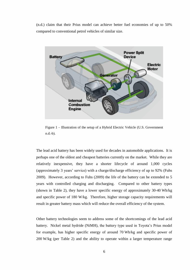
The technology works by combining a gasoline engine with an electric motor, as shown

in Figure 1. Current vehicles using HEV technology usually operate in parallel with the

gasoline powertrain. Therefore the gasoline engine and electric motor can provide

power independently, meaning that the gasoline engine can be shut-off to reduce fuel

consumption. During deceleration and braking an electric motor is used as a generator

to recover the kinetic energy. The electricity produced is stored in a battery for later

use. When the vehicle starts to accelerate again, an electric motor uses the stored

energy to accelerate or assist in accelerating the vehicle to reduce reliance on the

gasoline engine and hence fuel consumption. Toyota Motor Corporation Australia Ltd

6

(n.d.) claim that their Prius model can achieve better fuel economies of up to 50%

compared to conventional petrol vehicles of similar size.

Figure 1 – Illustration of the setup of a Hybrid Electric Vehicle (U.S. Government

n.d.-b).

The lead acid battery has been widely used for decades in automobile applications. It is

perhaps one of the oldest and cheapest batteries currently on the market. While they are

relatively inexpensive, they have a shorter lifecycle of around 1,000 cycles

(approximately 3 years’ service) with a charge/discharge efficiency of up to 92% (Fuhs

2009). However, according to Fuhs (2009) the life of the battery can be extended to 5

years with controlled charging and discharging. Compared to other battery types

(shown in Table 2), they have a lower specific energy of approximately 30-40 Wh/kg

and specific power of 180 W/kg. Therefore, higher storage capacity requirements will

result in greater battery mass which will reduce the overall efficiency of the system.

Other battery technologies seem to address some of the shortcomings of the lead acid

battery. Nickel metal hydride (NiMH), the battery type used in Toyota’s Prius model

for example, has higher specific energy of around 70 Wh/kg and specific power of

200 W/kg (per Table 2) and the ability to operate within a larger temperature range

7

(Fuhs 2009). However, the advantages of NiMH batteries come at a higher initial cost,

while battery life is also lower at approximately 600 cycles (2 years’ service) (Fuhs

2009). Furthermore, cooling also assists with faster recharge times (Fuhs 2009), which

is another design requirement.

The most promising technology for future rechargeable batteries is lithium-ion (Li-ion).

Capable of specific energy of 180 Wh/kg and energy density of 350 Wh/L (Fuhs 2009),

it requires less space and has less weight. Charge/discharge efficiency can also be as

high as 99% and the expected life of Li-ion is 4 years (Fuhs 2009). While it costs up to

50% more than NiMH, the expected lifecycle cost is lower according to Fuhs (2009). It

also has a lower self-discharge rate of around 5-10%/month compared to 3-20%/month

for lead acid and 30%/month for NiMH (per Table 2).

Whilst considered promising, Li-ion doesn’t come without its disadvantages. Li-ion

battery life suffers from calendar age, not just the number of cycles (Fuhs 2009),

meaning that capacity loss can occur due to aging. Battery durability is also affected by

operating and storage temperatures. Safety is another concern and careful control of

charging and discharging to avoid the potential of cells catching fire. In the event of

such instances, CO2 or dry chemical extinguishers are recommended over water

extinguishers.

Lead Acid NiMH Li-ion

Specific Energy (Wh/kg) 30-40 30-80 150-200

Specific Power (W/kg) 180 250-1000 300-1500

Energy Density (Wh/L) 60-75 140-300 250-350

Self-Discharge (%/month) 3-20 30 5-10

Consumer Price (Wh/$) - 1.37 2.80

C/D Efficiency (%) 70-92 66 99

Table 2 – Summary of battery performance properties for three battery types.

Sourced from Fuhs (2009).

8

The performance characteristics of the three battery types are summarised in Table 2.

The word ‘specific’ has been used to mean per unit mass and ‘density’ to mean per unit

volume. This is in alignment with the terminology used by Fuhs (2009). It has been

noted that while the values in the Table 2 have been reproduced from tables in Fuhs

(2009), he does occasionally refer to values that may differ deviate slightly from those

recorded in the tables.

An alternative to using batteries is to use a capacitor. A capacitor is a device that stores

electrostatic energy using an electric field. It has many advantages over batteries, the

first being that capacitors have higher efficiency, in the range of 90-98% (per Table 3).

This means that less energy is wasted because most of the energy stored can be

discharged. They also have higher storage and discharge speeds due to higher specific

power levels of up to 4kW/kg (Fuhs 2009). This provides an advantage in scenarios

requiring short bursts of high peak power (faster acceleration) and quick energy storage

(shorter braking distances).

Further, capacitors require less maintenance when compared with batteries and do not

deteriorate with use. They have an expected life in excess of 10 years and over 1

million discharge cycles (per Table 3), compared to batteries that have a life of up to 5

years and 10,000 discharge cycles. This means that replacement is less frequent and

generally costs less over time. However, the cost of capacitors compared to

conventional lead acid batteries is generally high, and won’t be considered competitive

until their cost drops below $5/Wh (Fuhs 2009). Another major problem with

capacitors is their low specific energy in the order of 1 to 10 Wh/kg (per Table 3).

Their low specific energy makes them unsuitable for long discharge times.

9

Batteries UCs

Lifetime w/o maintenance 1-5 years 10+years

No. in lifetime of high rate

discharge/charge cycles

1-000 – 10,000a

1,000,000b

C/D efficiency 40-80% 90%-98%

Charge time 1-5h 0.3-30s

Discharge time 0.3-3h 0.3-30s

Specific Energy (Wh/kg) 10-100 1-10

Specific Power (kW/kg) ~1 <10

Adequate energy to meet

peak power duration

Yes Yes

Limitation on SOC Low SOC limits life No effect SOC on life

Cost $/kWh Lead acid least; other than

types three to ten times

more

Slightly more lead acidc

Working temperatures -20 to +65 -40 to +65 a Depends on the application and BMS.

b Less dependent on application and monitoring.

c Significantly cheaper than all batteries except lead acid

Table 3 – Comparison of performance characteristics between batteries and ultra-

capacitors (Fuhs 2009).

1.1.3.2 Flywheels

Another method for recovering energy in regenerative braking is the use of flywheels.

Flywheels are mechanical devices used to store rotational energy. Figure 2 shows a

flywheel module in a containment housing. They work much to the same principles of

HEV. During braking, energy is recovered stored in the flywheel, while helping to

reduce vehicle velocity. As the vehicle slows down, the speed of the flywheel will

increase. When kinetic energy stored by the flywheel is transferred back into the

system, it helps to accelerate the vehicle while reducing the speed of the flywheel. This

puts less strain on the IC engine and therefore requires less power and reduces fuel

consumption.

10

Figure 2 – Diagram of a flywheel KERS module (Motor Trend Magazine 2014a).

The kinetic energy is transferred using a continuously variable transmission (CVT) unit

as shown in Figure 3. The CVT allows for a seamless transfer of energy to and from the

flywheel through an infinite number gearing ratios. A clutch is used to disengage the

flywheel when not in use.

The potential energy storage can be expressed by the equation:

𝐸 =1

2𝐽𝜔

2 [J] Equation [2]

Where 𝜔 is the angular velocity [rad/s] and 𝐽 is the mass moment of inertia [kg.m2].

From Equation 2 it can be understood that increasing the angular velocity will deliver

better results than simply improving the moment of inertia. This can be achieved using

the CVT unit.

11

Figure 3 – Flywheel KERS system layout (Motor Trend Magazine 2014b).

Flybrid Automotive Limited (2014) states that fuel consumption savings have been

demonstrated to be more than 18% over the New European Driving Cycle (NEDC) and

more than 22% in real world conditions. These statistics are supported by similar

claims by Volvo Car Group, who conducted joint tests with Flybrid Automotive. They

claim that the technology adds 80hp performance while reducing fuel consumption by

up to 25% (Volvo Car Group 2014).

Furthermore, the simplicity of the technology allows for long life spans with proper

maintenance. The life of some flywheels is designed to be more than 250,000 km with

no performance degradation (Flybrid Automotive Limited 2014). Flywheels can be

reliable with repeatable characteristics. The amount of energy stored at any given time

can be reliably measured by monitoring rotational speed.

Efficiency is another key characteristic. Physics dictates that transforming energy from

one source to another will inevitably incur losses. As flywheels store mechanical

energy using mechanical energy, conversion losses can be reduced. They can also

generate and absorb energy quickly. A mechanically driven flywheel can have an

12

overall charge/discharge efficiency of more than 70% during a full regenerative cycle in

stop start traffic (Body & Brockbank 2009 cited in Boretti 2010). However, due to the

relatively higher friction losses, flywheels tend to discharge at quicker rates making the

technology inefficient for storing energy for longer periods of time.

Flywheel systems also require safety design considerations. Increasing angular velocity

results in higher centrifugal stresses on the flywheel. If the speed of the flywheel

exceeds the design tensile strength of the material used, the flywheel will predictably

fail, releasing all of the stored energy instantaneously. Therefore, the flywheel housing

needs to be manufactured using materials that can safely withstand the energy during

failure and prevent flywheel material from breaching the housing; increasing the overall

mass of the system.

Increasing the weight of the flywheel results in greater moments of inertia, which

generally results in higher energy densities. However, more weight will result in greater

friction forces meaning energy losses and self-discharging. Furthermore, windage

losses caused by friction with the atmosphere contribute to the overall losses of the

system. In order to reduce these losses, manufacturers are now designing low friction

bearings using magnets and vacuum sealed housings; these can add to the overall cost

of the system.

1.1.4 Conclusion

In order to overcome the disadvantages of the technologies listed above, over the past

decade and a half, another technology has been gaining momentum in the literature.

Research and studies have been conducted into recovering kinetic energy using

compressed gas stored as potential energy. This can be achieved by either using the IC

engine as a compressor, or using a dedicated compressor much like the generator is used

in HEVs. The technology seeks to address the following problems:

1. Efficiency: One of the biggest problems associated with the recovery of kinetic

energy in HEVs is the efficiency of transforming one form of energy to another.

13

During energy recover, efficiency is reduced by the transformation from kinetic

energy into electrical energy using a motor or generator, which is then

transformed into chemical energy in a battery. These losses are also true for

discharging the energy back into the system. The other problem affecting

efficiency is the additional mass of KER system components. Additional mass

essentially reduces the global efficiency of the vehicle system due to energy

losses caused by friction.

2. Design Constraints: The available volumetric space within the engine

compartment causes design challenges. For flywheels, it limits the overall size

of the device and the mounting points available. In HEVs it demands efficient

use of the space due to the addition of several components. The position of the

mass of the additional components must also be considered. It can cause a

change in vehicle dynamics such as braking and cornering.

3. Safety: Working with electricity introduces new safety requirements within

automobiles. High voltages used in regenerative braking systems are a major

health and safety concern, particularly if the vehicle is involved in an accident.

Furthermore, although generally considered safe, batteries are produced using

hazardous materials. The risks are relevant for both the handling and disposing

of damaged batteries. For example, lead is a toxic material that can cause

serious health issues in high levels. Cadmium is also considered more toxic than

lead and can cause health problems if a person is exposed to the metal for a

prolonged time.

Concept 1.2

The concept of this research is to use a conventional IC engine to recover kinetic energy

of a motor vehicle during braking. It proposes that the kinetic energy recovered would

be converted to potential energy, stored as compressed gas using a high pressure vessel.

During acceleration, the stored energy would be used to reduce with the goal of

reducing fuel consumption.

14

Depending on how the recovered energy is used, the IC engine may have one or two

additional operational modes. The first would be a pneumatic pump mode. During the

braking phase, the IC engine would be used as a reciprocating compressor powered by

the kinetic energy of the vehicle due to its motion. Air would be pumped by the engine

to a pressure vessel and stored until required. This should reduce the need for any

major additional components.

If the compressed air is used to supercharge the engine, it may not require a second

operation mode. However, the air could be used to power a pneumatic motor.

Alternatively, a second additional operation mode may be used - pneumatic engine

mode. Given sufficient air pressure, this mode uses the potential energy to accelerate

the vehicle or provide more torque during acceleration. Using the recovered kinetic

energy could potentially reduce the fuel needed to accelerate the vehicle under

conventional operating conditions.

Aims and Objectives 1.3

The aim of this project is to evaluate the plausibility of recovering the kinetic energy of

a motor vehicle by using the internal combustion engine to compress gas. Specifically,

the aim of the project can be divided into several significant objectives characterised as

follows:

Understand current kinetic energy recovery technologies including their

respective benefits and weaknesses to establish a suitable benchmark for

comparison;

Determine the ability to use an internal combustion engine to produce

compressed gas. Critically analyse the similarities and divergences with positive

displacement compressors and identify any significant design deviations that

may need to be addressed;

Determine the practical and feasible uses for the compressed gas within motor

vehicles and analyse the effects on performance;

Measure the energy recoverable using compressed gas using a numerical model,

with appropriate assumptions, created to simulate an IC engine operating as a

compressor; and

15

Analyse the results, comparing key performance parameters with current

technologies and conclude on the viability of compressed air as an alternative.

Scope 1.4

The research undertaken in this project focuses specifically on passenger automobiles

powered by naturally aspirated internal combustion engines. The internal combustion

engine considered will be a SI four-stroke piston engine. As a result, this specifically

excludes automobiles powered by Wankel engines (rotary), diesel engines employing

Homogenous Charge Compression Ignition (HCCI) and other stroke configurations

including two-stroke engines.

The energy recovery analysis within this report is limited to the operating conditions of

automobiles and the potential energy recoverable that is directly related to systems

under these conditions. The project will not undertake an energy cost analysis,

therefore the energy expended to manufacturing additional components needed to

recover kinetic energy versus the energy recoverable.

16

2 Literature Review

Internal Combustion Engine as a Compressor 2.1

2.1.1 Introduction

The purpose of a compressor is to increase the pressure of a gas and store this gas as

confined kinetic energy. Understanding how compressors work is pertinent to

establishing the feasibility of using an IC engine as a compressor. For this reason the

following section will focus on comparing the characteristics of modern compressor

technology with that of an IC engine. While many types of compressors exist in the

market place, this analysis will concentrate on comparisons with a reciprocating

compressor (a positive displacement compressor) due to their similar functionality. It

will compare and contrast their operating cycles, componentry and discuss any potential

performance limitations.

2.1.2 Ideal Operating Cycles

The following section will compare and contrast the ideal operating cycles of a

reciprocating compressor and a four-stroke IC engine.

2.1.2.1 Ideal Positive Displacement Compressor Cycle

The simplest way to estimate performance is to use a thermodynamic cycle. The

analysis uses the ideal gas laws and a set of assumptions to simplify the actual process.

Under the ideal compression cycle, the process is assumed to be isentropic. This

implies that the process is adiabatic and that no heat will transfer from the control

volume to the outside, meaning no losses due to heat transfer and friction.

The ideal compression cycle is illustrated in Figure 4a and Figure 4b. The figures

display the pressure compared to the volume of the cylinder (P-V diagram), at each

crank angle.

17

Figure 4 – Ideal compression cycle and pressure-volume diagram of a reciprocating

compressor showing the four processes. Sourced from (Hanlon 2001).

At point 1, the piston starts at bottom dead centre (BDC) and maximum cylinder

volume. At BDC the gas in the cylinder is at suction pressure. As the crank turns, the

piston starts to move upwards decreasing the volume of the cylinder and compressing

the gas. This decrease in volume causes the gas to increase in both temperature and

pressure (process 1-2) at an exponential rate. This process can be considered as

adiabatic and reversible.

The process continues until the pressure in the cylinder equals the discharge pressure at

point 2, causing the discharge valve to open. After point 2, the pressure in the cylinder

remains constant while the piston continues to displace the gas into the discharge line.

This process is considered isobaric and isothermal.

This continues until the crank angle reaches top dead centre (TDC) at point 3 and the

valve closes. At this point, the residual gas left in the clearance volume begins to

expand back to suction pressure – decreasing in pressure (process 3-4) and in

temperature. The expansion process is considered adiabatic and reversible.

18

At point 4 the pressure in the cylinder equals the suction pressure, which is usually

close to the atmospheric pressure surrounding the compressor. The suction valve opens

and the volume of the gas in the cylinder increases until the crank angle reaches BDC.

The intake process 4-1 is isobaric and isothermal at intake pressure and temperature.

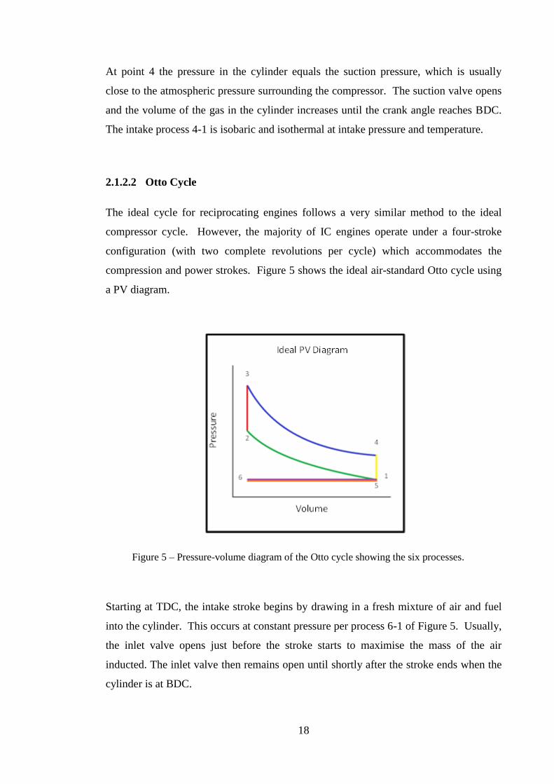
2.1.2.2 Otto Cycle

The ideal cycle for reciprocating engines follows a very similar method to the ideal

compressor cycle. However, the majority of IC engines operate under a four-stroke

configuration (with two complete revolutions per cycle) which accommodates the

compression and power strokes. Figure 5 shows the ideal air-standard Otto cycle using

a PV diagram.

Figure 5 – Pressure-volume diagram of the Otto cycle showing the six processes.

Starting at TDC, the intake stroke begins by drawing in a fresh mixture of air and fuel

into the cylinder. This occurs at constant pressure per process 6-1 of Figure 5. Usually,

the inlet valve opens just before the stroke starts to maximise the mass of the air

inducted. The inlet valve then remains open until shortly after the stroke ends when the

cylinder is at BDC.

19

The compression stroke begins when both valves are closed at point 1. In the Otto cycle

the compression is regarded as isentropic as an approximation to the real IC engine.

The gas inside the cylinder undergoes compression (process 1-2) until combustion is

initiated by an electric discharge across the spark plug at point 2.

The combustion process is considered to be a constant-volume heat input process shown

as points 2-3. The gases in the cylinder increase rapidly in both temperature and in

pressure. This occurs between 10 and 20 crank angle degrees before TDC (Heywood

1988).

Next, the expansion (power) stroke begins when the cylinder reaches TDC and peak

pressure at point 3. The high pressure and enthalpy values of the gas thrust the cylinder

down forcing the crank to rotate. The Otto cycle assumes this process is isentropic.

Pressure then decreases and the volume increases (process 3-4) until the stroke ends

when the cylinder reaches BDC. Just before this point, the exhaust valve opens to begin

the exhaust stroke.

When the exhaust valve opens, blowdown is experienced and the pressure in the

cylinder drops until the pressure equalises with the exhaust pressure. The process is

approximated assuming a closed system, constant-volume pressure reduction from

points 4-5.

As the piston travels back up the cylinder, the remaining exhaust gases exit the cylinder.

The Otto cycle assumes a constant pressure at atmospheric pressure (process 5-6). As

the piston approaches TDC, the inlet valve begins to open once more to start the cycle

again while the exhaust valve closes just after TDC.

2.1.2.3 Operating Analysis

The previous section illustrates the similarities and differences between the ideal

compression cycle and the Otto cycle. The key comparisons are the intake,

compression and expansion processes. However, due to the difference in stroke

20

configuration (two-stroke for the compressor and four-stroke for the engine), these

processes do not follow the same operational sequences.

The removal of certain processes will be necessary for operating the IC engine as a

compressor. While the combustion process in the Otto cycle is fundamental during

conventional operation of the engine, it is not required in the compression cycle, as this

process adds no value. Removing this process will not only reduce fuel consumption,

but also reduce the losses that occur during the blowdown process. As an example of

switching off the combustion process, simulations performed by Dönitz et al. (2009a)

demonstrated that fuel savings of 6% could be achieved by adding a stop/start capability

to an engine for the NEDC test cycle. Furthermore, the exhaust process needs to be

replaced with the charging process. Therefore, instead of discharging the gases to the

atmosphere, the gas would be discharged to a storage tank.

Equally important is removing the second revolution, allowing the engine to operate in

a two-stroke configuration. Otherwise, the gas would unnecessarily undergo a second

compression and an expansion process. While these processes would not add any work

under the ideal cycle, it also would not be the most efficient way of recovering kinetic

energy as compressed gas would only be accumulated every second revolution.

Accordingly, an appropriate solution would be required to allow the engine to operate

as a compressor. The solution must address the stroke configuration, the removal of the

combustion (and hence the blowdown) and exhaust processes, and the addition of a

charging process. Henceforth, the discussion on potential losses during compression is

based on the assumption that a suitable solution exists.

2.1.3 Real Losses

The isentropic process assumed by the ideal compression cycle infers that no losses

occur within the system. Although this outcome would be ideal, the laws of physics

dictate that this is unachievable. The main losses associated with all compressors are

21

caused by heat transfer, flow losses and leakage. These losses are also apparent in IC

engines.

Furthermore, with the assumption that the combustion process is removed during

braking, we can exclude losses due to finite combustion timing, exhaust blowdown and

incomplete combustion due to their irrelevance during operation as a compressor.

Figures 6a and 6b show the pressure-volume diagrams of a reciprocating compressor

with suction and discharge losses. The shaded areas in the figures indicate, during the

charging and intake processes, where some of the losses can occur.

Figure 6 – Pressure-volume diagram of a compressor with approximate suction and

discharge losses (Hanlon 2001).

2.1.3.1 Heat Transfer in Compressors

Heat transfer is inevitable in the compression cycle and will affect compressor

performance. The cylinder walls and the piston will operate at a temperature

somewhere between the suction temperature and the discharge temperature (Hanlon

2001). This temperature can be considered steady even with the fluctuating

temperatures of the gas during the cycle (Hanlon 2001). However, the temperature of

the cylinder wall will not be uniform, particularly around the intake and discharge

(a) (b)

22

valves, which makes calculating the effects of heat transfer imprecise and problematic.

Furthermore, the temperature of the intake port and discharge lines will also have an

effect on the overall performance of the system due to flow restrictions (Hanlon 2001).

In compressors, the most influential effect of heat transfer occurs during the intake (or

suction) process (Hanlon 2001). During this process, heat is added to the gas as it flows

through the suction passage and through the valve, reducing the density of the gas.

Without any change in pressure, this will result in a decrease in the mass flow

compressed and hence reduce the efficiency of the system.

Dynamic heat transfer also occurs during the compression stroke (Hanlon 2001).

During the initial phase of the stroke, the cylinder wall is at a higher temperature than

the gas – meaning heat is transferred to the gas which results in increased pressure and

temperature. During the second phase of compression, the heat of the gas elevates to

temperatures above the cylinder wall – meaning heat is transferred to the cylinder wall

and the gas loses temperature and pressure. Hanlon (2001) suggests that the net effect

of the heat exchange during the compression stroke is a slight reduction in capacity.

This is due to the cylinder wall being closer to suction temperature, as the gas in the

cylinder spends more time at or near suction temperature.

2.1.3.2 Heat Transfer in IC Engines

Perhaps one of the greatest differences compared to compressors is the operating

temperatures of an engine. According to Pulkrabek (1997) the hot intake manifold

increases the temperature of the air by approximately 25-35°C. Without an increase in

pressure, this lowers the density of the incoming air which reduces volumetric

efficiency. Pulkrabek (1997) states that at lower engine speeds, this effect is magnified

as the air remains in the intake manifold for longer periods of time due to lower mass

flow rates.

For compressor operations, the convective heating caused by the intake manifold is not

ideal. However, the intake manifold is sometimes purposely heated by design.

23

Increasing the air temperature can enhance fuel evaporation resulting in a more

homogenous mixture (Pulkrabek 1997). This is important when the IC engine is

operating under normal conditions and not as a compressor. Henceforth, any solution to

reduce these heating effects must also consider the underlying intake manifold design

during normal operating conditions.

The other important form of heat transfer occurs in the cylinder. The cylinder

temperatures of an IC engine are much higher than those in a reciprocating compressor

due to the combustion process. Figure 7 illustrates the typical temperature distribution

within an SI engine operating at steady state. The highest temperatures occur around

the spark plug, piston face and exhaust components. However, the component with the

greatest area in the cylinder is the cylinder walls. Pulkrabek (1997) states that the

temperature of the wall should not exceed 180°-200°C.

Figure 7 – Typical temperature values found in an SI engine operating at normal

steady state conditions. Temperatures are in degrees C (Pulkrabek 1997).

When the air enters the cylinder, convective heat transfer occurs from the cylinder to the

gas. According to Pulkrabek (1997) and Heywood (1988), the convection heat transfer

24

coefficient will vary greatly due to factors such as turbulence, swirl and velocity.

However, perhaps the most popular correlation for determining the overall heat transfer

coefficient is that produced by Woschni (1967). This is shown in Equation 3.

ℎ𝑐 = 3.26𝐵−0.2𝑝0.8𝑇−0.55𝑤0.8 [W/(m2∙K)] Equation [3]

Where 𝐵 is the diameter [m] of the piston, 𝑝 is the average gas pressure [kPa], 𝑇 is the

temperature [K] and 𝑤 is the average gas velocity [m/s].

The average gas velocity can be related to the mean piston speed by the equation:

𝑤 = [𝐶1𝑆�̅� + 𝐶2𝑉𝑑𝑇𝑔

𝑝𝑔𝑉𝑔(𝑝 − 𝑝𝑚)] [m/s] Equation [4]

This equation can be further simplified where 𝐶1 = 2.28 and 𝐶2 = 0 for the intake,

compression and exhaust processes.

𝑤 = [𝐶1𝑆�̅�] [m/s] Equation [5]

Woschni (1967) also attempted to account for the gas velocities induced by combustion

during the combustion and expansion processes. However, as combustion won’t take

place during compression mode, the expansion process could be estimated by the same

heat transfer coefficients.

Heat transfer from the cylinder to the gas is important for keeping the cylinder walls

cool and within design temperatures. Under closed boundary conditions, the addition of

heat to the gas increases the energy of the system. While it is not expected that a

significant amount of heat will be transferred given the time the air spends in the

cylinder, it would serve to increase the overall efficiency by recovering this heat that

would otherwise be dissipated into the ambient environment.

25

2.1.3.3 Compressor Valve Timing

Valves are one of the most critical components in reciprocating compressors (Hanlon

2001). A key reason for this is the effect on the reliability of a compressor. Valves are

required to function under harsh operating conditions. They are also required to operate

in a highly corrosive environment with dirty gases and residues that can build up at the

inlet and discharge valves. This is critical given that opening and closing times are

measured in milliseconds and are required to have a life of more than a billion cycles

(Hanlon 2001).

Valve performance is also affected by timing. Reciprocating compressors generally use

check valves to restrict the flow to a single direction (Hanlon 2001). Due to inertia,

these valves do not open and close instantaneously as assumed by an ideal valve.

Therefore, valves do not stay at full lift for the entire duration of the charging and intake

processes.

The spring of the valve affects the capacity of the compressor. If the spring of the valve

is too heavy, the valve will close too early. This means that the average valve flow area

during the intake and charging processes will be reduced. If the valve spring is too

light, it can result in the valve not closing at dead centre, which is the optimal timing

according to Hanlon (2001) – TDC for the discharge valve and BDC for the suction

valve.

2.1.3.4 IC Engine Valve Timing

Compared to compressor valves, the intake and exhaust valves are commonly operated

mechanically using a cam shaft and spring loaded poppet valves.

Valve timing

Valves are opened and closed at a rate sufficient enough to avoid noise and excessive

cam wear (Pulkrabek 1997). Comparable to compressors, valves are not at full lift for

the entire process. For this reason engine valve timing ensures that the valves are fully

open at peak piston velocity (Pulkrabek 1997). Unfortunately, a consequence of this

26

can be the overlapping of valves. Valve overlap occurs when the intake and exhaust

valves are open at an instant in time. It arises when the intake valve is opening and

exhaust valve is closing. While it is an issue in combustion engines, it should not be a

concern while operating in compression mode.

Opening intake valve before TDC

The opening of the intake valve is designed to be fully open at TDC when the intake

stroke begins in order to maximise air intake (Pulkrabek 1997). For this to happen, the

valve must start to open at 10 to 25° before TDC (Pulkrabek 1997) due to the finite

opening speeds. During compression mode, the intake valve will open much later after

the expansion process has finished. In compressors, this is controlled by the pressure

differential (between the pressure in the cylinder the intake pressure) and the heaviness

of the spring (Hanlon 2001). It is currently unclear whether or not the intake valve

should open before pressure in the cylinder reaches intake pressure to maximise air

intake. The consequence of opening too early is that air in the cylinder could escape

back into the intake manifold due to the cylinder pressure being higher than intake

pressure.

Closing intake valve after BDC

The closure timing of the intake valve affects the amount of air accumulated in the

cylinder (Pulkrabek 1997). In an engine, the intake valve is not fully closed until after

BDC. According to Heywood (1988) the intake valve can remain open until 50 to 70°

after BDC to allow the air to continue to flow into the cylinder. This is in contradiction

to the closing timing of the intake valve for compressors as specified by Hanlon (2001).

It is assumed that this is due to the difference in the type of valves used. Unlike check

valves, poppet valves do not rely upon pressure differentials and therefore provide more

timing flexibility.

During intake, a pressure differential exists even when the piston reaches BDC and air

still flows into the cylinder. The air continues to enter until it is compressed to equalise

with the intake pressure. This is the optimal time for the intake valve to close according

to Hanlon (2001), who states that volumetric efficiency will be reduced if the valve

27

closes too early. However, if the valve closes too late, air will be forced back through

the intake manifold with the same effect on volumetric efficiency (Hanlon 2001).

Pulkrabek (1997) states that the optimal valve closing point is highly dependent on

engine speed. Higher speeds require later closing times due to the greater pressure drop

across the intake valve caused by higher mass flow rates of air, while earlier closing

positions are more ideal for lower speeds with smaller pressure differentials.

Closing exhaust valve after TDC

Similar to the intake valve, the exhaust valve remains fully open until TDC to ensure

the maximum amount of exhaust is displaced out of the cylinder chamber. Furthermore,

it also reduces the back pressure on the cylinder head which can reduce the total

efficiency of the engine. Closing therefore begins very close to TDC which means total

closure doesn’t occur until 8 to 50° after TDC (Pulkrabek 1997).

The closure timing of the exhaust valve could be compared with the valve closure

timing required for the tank charging process when operating in compression mode.

Again, the optimal closure timing stated by Hanlon (2001) conflicts with the timing of

the exhaust valve for an IC engine. Adding to the complexity of this however is the

difference in exhaust pressure and the pressure of the air storage tank. Therefore, at

higher tank pressures, it could be expected that TDC is the optimal closure timing.

However, at lower tank pressures, it may depend on engine speed.

2.1.3.5 Compressor Flow Losses

When dealing with the flow of gases through pipes, the gas will always experience

losses to some extent. A loss of flow rate due to fluid friction is one source of losses,

along with choked flow which can occur in high speed flows. Furthermore, due to the

intermittent flow nature of reciprocating compressors, a pulsating flow can occur which

leads to pressure losses.

28

The unsteady nature of the gas inflow and outflows from the compression cylinder

causes pulsations in the suction and discharge piping. Should the amplitude of the

pulsation levels be sufficient, this can affect the valve open and close timing (Hanlon

2001). This can cause the average inlet and discharge pressures to deviate from design

pressures and result in power and capacity values differing from performance standards,

either favourably or adversely.

Additionally, gas flowing through a restriction will experience a pressure drop due to

the increase in velocity caused by the restriction. This is evident in Benoulli’s equation

for incompressible flows. This can be exacerbated by valve restriction, commonly

caused by the build-up of solids, improper springing of valves, pulsation of gasses and

design inefficiencies.

2.1.3.6 IC Engine Flow Losses

Fluid Friction Losses

When air flows through passages it undergoes a pressure drop due to a viscous flow

friction (Pritchard 2011). The pressure entering the cylinder will therefore be less than

the surrounding atmospheric air pressure resulting in a reduction of volumetric

efficiency. The pressure drop effect is worsened by flow restrictions that can be found

in the engine intake system of a motor vehicle. These restrictions include the air filter,

throttle plate, intake manifold and intake valve. The viscous drag caused by these

components increases with the square flow velocity, as shown by Heywood (1988) in

Equation 6, where the total quasi-steady pressure loss due to friction can be related to

the mean piston speed. Heywood (1988) states that the intake pressure can be 10 to 20

% lower than atmospheric when the piston is moving at close to its maximum speed.

𝑝𝑎𝑡𝑚 − 𝑝𝑐 = 𝜌𝑆�̅�2 ∑ 𝜉𝑗 (

𝐴𝑝

𝐴𝑗)

2

[Pa] Equation [6]

Where, 𝑝𝑎𝑡𝑚 is the atmospheric pressure [Pa], 𝑝𝑐 is the cylinder pressure [Pa], 𝑆̅ is the

mean piston speed [m/s], 𝜉𝑗 is the resistance coefficient for the component, and 𝐴𝑝 and

29

𝐴𝑗 represent the piston area [m2] and the component minimum flow area [m

2]

respectively.

Besides designing the intake to reduce restrictions, one method to reduce these effects is

to increase the diameter of the intake manifold. Flow velocity will be decreased and

pressure losses can be reduced. However, Pulkrabek (1997) notes that a decrease in

velocity will also result in poorer mixing of the air and fuel along with less accurate

cylinder-to-cylinder distribution.

An alternate solution proposed is to use a variable intake system. These have been used

to optimise SI engine performance including improvements in fuel efficiency (Ceviz &

Akin 2010) by varying the intake plenum length/volume. Usually this is achieved with

the use of two separate intake ports governed by valves to two different manifolds with

different lengths. Alternatively a single path runner system with variable lengths using

mechanical methods could also be used. The shorter manifold used at higher engine

speeds to deliver maximum power would help reduce pressure losses associated with

fluid friction and improve volumetric efficiency for compressing air.

Valve Flow Losses

The losses across the valves in an engine will be different to those experienced by

reciprocating compressors. This is due to the difference in geometry between poppet

valves and reed valves. The mass flow rate across a poppet valve can be estimated by

Equation 7 (Heywood 1988). This equation shows that the mass flow rate �̇� [kg/s] is

related to a change in pressure across the valve.

�̇� =𝐶𝐷𝐴𝑅𝑝0

(𝑅𝑇0)2 (𝑝𝑇

𝑝0)

1/𝛾

{2𝛾

𝛾−1[1 − (

𝑝𝑇

𝑝0)

(𝛾−1)/𝛾

]}1/2

Equation [7]

Where 𝛾 is the specific heat ratio. The flow rate is related to the upstream stagnation

pressure 𝑝0 [Pa] and the stagnation temperature 𝑇0 [K], which is the intake system gas

state for flow through the intake valve, and the cylinder gas state for flow through the

exhaust valve; the downstream pressure 𝑝𝑇 [Pa] which is the cylinder pressure for flow

through the intake valve, and the exhaust pressure for flows through the exhaust valve;

30

and the reference area 𝐴𝑅 [m2] which is a characteristic of the valve design. The

discharge coefficient 𝐶𝐷 allows for the real gas flow effects and is usually determined

experimentally.

Due to finite valve opening and closing speeds, flow losses will be higher due to

reduced flow areas. Figure 8, illustrates the change in flow area caused by valve lift as

a function of crank angle. Figure 8a shows the valve lift in centimetres compared to the

camshaft angle on the x-axis. Figures 8b and 8c show the flow area in cm2 with respect

to the income and exhaust valves respectively. Therefore it would be expected that

valves with quicker lift times will increase the time at maximum flow area and reduce

flow losses.

Figure 8 – Valve-lift curve showing the minimum intake and exhaust flow area as a

function of crank angle (Asmus 1982).

Choked flow

Choked flow occurs in IC engine systems when a maximum flow rate is achieved and

cannot be increased even with a change in downstream conditions. High air flow

31

velocities eventually reach sonic velocity at some point in the intake system, usually the

most restricted passage such as the intake valve. The effect of this limiting condition is

a decrease in efficiency at higher speeds.

Flow pulses

Unlike compressors, the pulsed gas flow in engines will not have an effect on valve

timing. This is due to the valves being controlled mechanically. Instead, the pressure

waves created can affect volumetric efficiency (Pulkrabek 1997). Pulkrabek (1997)

explains that the wavelength is dependent on pulse frequency and flow rate or velocity.

When waves reach the end of the manifold or an obstruction, they create a reflected

pressure wave. This reflected pressure wave travels in the opposite direction and

interacts with the primary wave. In phase pressure waves that reinforce at the intake

valve will result in pressure pushing the air into the cylinder, increasing volumetric

efficiency (Pulkrabek 1997). Out of phase pressure pulses result in reduced pressure

pushing air into the cylinder and lower volumetric efficiency.

The solution proposed by Pulkrabek (1997) is to use active intake systems which adapt

to different engine speeds. For example, a single path manifold with variable length or

a dual path system with or without secondary throttle plates. This solution is supported

by experimental research undertaken by Ceviz (2007), who showed that a variation in

the plenum volume caused an improvement on both engine performance and pollutant

emissions at different speeds.

2.1.3.7 Leakage

Leakage is common in all compressors in some form. While the magnitude of these

leakages varies to some extent, it will always have a negative impact on efficiency.

Hanlon (2001) states that the general leakage paths in reciprocating compressors occur

around the piston rings and the valves which do not form a perfect seal to prevent

reverse flow.

Hanlon (2001) explains that leakage through the suction valve has two effects. First, it

causes hot gas to enter the inlet passage. This is essentially equivalent to heat transfer,

32

therefore reducing gas density and reducing efficiency. Secondly, it directly results in a

loss of the compressed gas. This is also the effect of discharge valve leakage. Gas

previously compressed is wasted as it escapes back into the cylinder. This will decrease

the mass flow compressed without any decrease in the power into the system.

As the designs of SI four-stroke piston engines are similar to reciprocating compressors,

they will also experience small losses due to leakage. Increased cylinder pressure can

result in unwanted gas flow into crevices such as between the piston and piston wall and

also through the piston rings. Pulkrabek (1997) states that leakage in a properly

designed and well maintained engine is small and usually only accounts for less than

one percent of the cylinder volume. However, with the addition of an air storage tank

the losses may slightly increase if the valve to the charging line is not sealed

sufficiently.

2.1.3.8 Mechanical Frictional Losses

Friction in engines reduce the amount of power delivered to the wheels and is dissipated

as heat. The work produced per cycle is marginally consumed to overcome the friction

which is the result of adjacent components rubbing against each other. In comparison,

during compression the friction reduces the amount of power available to compress the

air which reduces efficiency of the system. Sources of friction can include friction due

to the engine, transmission and drivetrain.

The friction mean effective pressure (FMEP) can be calculated using Equation 8. The

equation is a correlation based on the data collected by Barnes-Moss (1975) (cited in

Heywood 1988) for the total motoring friction for four-stroke SI engines with a

displacement between 845 and 2000 cm3 at wide open throttle. The correlation has

been adjusted for a two-stroke cycle with the output in [Pa] as opposed to bar.

𝐹𝑀𝐸𝑃 = [0.97 + 0.15 (𝑁

1000) + 0.05 (

𝑁

1000)

2

] ∙105

2 Equation [8]

Where 𝑁 is the engine speed in revolutions per minute.

33

Applications of Compressed Gas 2.2

2.2.1 Introduction

The literature reveals that there are two main areas for which compressed gases has

useful application in automobiles. These are:

Supercharging; and

Pneumatic Engines.

While each of these has different operations, fundamentally they both serve the purpose

to improve vehicle performance through efficiency and a reduction in emissions. These

will now be individually discussed in greater detail.

2.2.2 Supercharging

Supercharging is not a new concept. Two types of supercharging technologies are used

in many of the motor vehicles on our roads today: superchargers and turbochargers.

Both are used to increase the intake pressure supplied to the IC engine. The increased

intake pressure results in more air and fuel (for a given air/fuel ratio) into the

combustion chamber each cycle. The additional air and fuel results in an increase in the

net power output (or work done) and has also been shown to increase volumetric

efficiency. In addition, it means that smaller engines can be used which can result in

decreased fuel consumption.

The turbocharger essentially works like a centrifugal compressor. Mounted in the

exhaust flow of the engine, the exhaust gases are used to spin the turbine (usually a

radial inflow turbine) which in turn drives the centrifugal compressor. As the pressure

in the exhaust system is only slightly higher than atmospheric pressure, only a very

small pressure drop can occur. For this reason, it is necessary to operate the turbine at

high speeds which requires design consideration to ensure safety and reliability.

34

The major advantage of turbochargers is that the compressor is driven only by waste

energy in the exhaust. Therefore, very little of the useful energy produced by the engine

is used to power the compressor. However, the disadvantage of using the exhaust to

drive the compressor is the occurrence of turbo-lag. This refers to the slow response to

torque demand at low engine speeds. It consequently requires several engine cycles

before the change in exhaust flow is at a rate sufficient to accelerate the turbine to

produce the desired inlet pressure.

A solution to the issues associated with turbocharging is highlighted by Dönitz et al.

(2009a). Using a hybridized IC engine to compress air (therefore the ability to alternate

between normal operation and a compressor mode), the stored air can be used in a

manner that allows the design of turbochargers to be focused entirely on engine

efficiency. The research conducted by Dönitz et al. (2009a) focused on fuel

consumption using a dynamic programming technique. The results of their research

showed that engine hybridization combined with downsizing a turbocharged engine and

cylinder deactivation can save as much as 34% fuel. They concluded that engine

downsizing was the most important contributing factor in overall fuel consumption.

Superchargers on the other hand, compress air using a positive displacement system, the

two most common being a screw type compressor or a lobe pump. The compressor is

mechanically driven by either a belt, chain or gears directly off the engine crankshaft.

Ultimately, the mechanical drive of the supercharger is both its biggest advantage and

greatest downfall. The major advantage is the very quick response times to throttle

changes. Supercharged engines do not suffer the lag experienced by turbochargers as

the change in engine speed is immediately transferred from the crankshaft to the

compressor. However, the power to drive the compressor is essentially a parasitic load

much like air conditioning.

Alternatively, the compressed air accumulated in a high pressure tank could be used as a

direct alternative to superchargers and turbochargers. This would overcome the

parasitic effect of the supercharger, the lag associated with turbochargers, along with the

additional weight associated with each system. One method for achieving this is

35

explained by Higelin, Charlet and Chamaillard (2002) and illustrated in Figure 9.

During the compression process (1-2 in Figure 9), the charge valve can be opened to

add an additional compression step to the process as illustrated in process 10-11 in

Figure 9. Higelin, Charlet and Chamaillard (2002) explain three main differences this

strategy offers:

1. Using the conventional intake stroke, the life of the high pressure tank air charge

can be enhanced (2 to 4 times) as the amount of air displaced only needs to be in

excess of the cylinder charge at atmospheric pressure.

2. A higher high-pressure cycle IMEP due to the dual stage compression stroke. It

can be further maximised by opening the charge valve as late as possible while

closing when the cylinder pressure reaches tank pressure.

3. Adversely, the higher exhaust pressure compared to the intake pressure means

that the low-pressure cycle IMEP is negative.

Figure 9 – Idealised pressure-volume diagram of an engine with the option of

charging an air tank during the compression process (Higelin, Charlet &

Chamaillard 2002).

The main problem associated with the increase in the intake air pressure is the increase

in air temperature caused by the compressive heating. Higher intake temperatures result

in higher gas temperatures during the whole cycle, particularly during the compression

36

stroke. This is undesirable in SI engines as it can cause self-ignition and knocking

problems. In order to avoid this, cooling mechanisms such as intercoolers can be used

to lower the temperature of the newly compressed air. However, the introduction of

these systems can add to design issues due to space constraints and losses caused by the

additional weight.

2.2.3 Pneumatic Engines

Two different types of systems have been theorized and tested: a pneumatic engine

operation mode using the IC engine, and a hybrid pneumatic power system.

2.2.3.1 Pneumatic Engine Operation (Hybridized IC Engine)

Under this concept, an additional operating mode of the IC engine is considered. It

assumes that the engine can operate as either a conventional IC engine or a pneumatic

motor powered by compressed air. The pneumatic motor operation cycle is illustrated

in Figure 10. It follows a two-stroke configuration that can lead to higher torque

outputs as well as lower friction losses (Higelin, Charlet & Chamaillard 2002).

Figure 10 – Ideal pressure-volume diagram of an engine operating as a pneumatic

motor (Schechter 1999).

The first step is cylinder charging (process 1-1’ of Figure 10). The charging valve

opens at point 1 allowing the compressed air to discharge into the cylinder until the

cylinder pressure reaches the tank pressure at point 1’. This process occurs at constant

volume and is assumed to be adiabatic. Discharge continues from process 1’ to 2 at

constant pressure under the assumption that the process is isobaric.

37

The second step is cylinder expansion (process 2-3). The charging valve is closed from

points 2 to 3 and the air charge expands in the cylinder. The process produces work and

forces the piston down. This process is considered adiabatic and reversible. It is

important to note that the closure timing of the charging valve should be selected to

ensure that full expansion takes place until pressure reaches atmospheric pressure. If

the timing is not controlled, losses could occur, much like the blowdown process when

the exhaust valve opens after expansion in a four-stroke engine.

The final step is the exhaust stroke (process 3-1). The exhaust valve opens at point 4

allowing the cylinder to discharge into the exhaust system until it reaches atmospheric

pressure (or exhaust pressure). Alternatively, Schechter (1999) says that the air could be

expelled through the intake valve to avoid excessive cooling of the catalyst. The

potential energy of the air at point 4, but can be managed by optimising the closure

timing of the charging valve. The remaining air is expelled during process 4 to 1 which

is considered isobaric.

Using the IC engine to compress air while braking and in a pneumatic motor mode

during acceleration, several researchers concluded that efficiencies could be achieved.

Simulations performed by Higelin, Charlet and Chamaillard (2002) showed a reduction

of around 15% of the global fuel consumption without system optimisation.

Furthermore, Trajkovic et al. (2007) reported regenerative efficiencies of up to 33%,

where regenerative efficiencies is defined as the ratio between the positive IMEP and

the negative IMEP of the pneumatic motor and compression modes respectively. It has

been noted however that the simulations performed by Higelin, Charlet and Chamaillard

(2002) were based on real world simulations while Trajkovic et al. (2007) focused on

controlled simulations with some optimisation. The results are therefore difficult to

compare.

Another similar method that has been considered was introduced by Schechter (1999),

called the Air-Power-Assist (APA) cycle. This cycle can operate in both a two-stroke

and a four-stroke operation, however for the purposes of this analysis we will only

consider the four-stroke operation as illustrated in Figure 11. Under this cycle the

38

engine continues to operate as an IC engine. The main difference is that the high

pressure tank delivers a charge of compressed air during the intake stroke at point 1 in

Figure 11. The air expands and performs work on the cylinder head causing

displacement. The charging valve then closes at point 3. This air charge is then used in

the combustion process. This part of the cycle is comparable to that in Figure 10.

Figure 11 – Pressure-volume diagram of the Air-Power-Assisted cycle for a four-

stroke cycle (Schechter 1999).

The advantage of the APA cycle is the work performed by the compressed air

supplements the work performed by combustion in the other cylinders while reducing

pumping losses. Thus reducing work needed to be performed by the combustion

process, which means that the fuel consumption could potentially be reduced.

Furthermore the APA cycle allows for higher engine torque during acceleration.

The mathematic model used by Schechter (1999) to demonstrate the performance of the

cycle resulted in a reduction in fuel consumption by more than 50% when compared to

a conventional engine. Further work conducted by Tai et al. (2003) used the APA cycle

to model and calculate savings under typical city and highway driving conditions. The

air hybrid model reported a 38% reduction in fuel consumption (Tai et al. 2003). The

APA cycle was taken one step further by Kang et al. (2008) who demonstrated that the

39

APA cycle could be implemented into an engine system for use in heavy duty

applications.

2.2.3.2 Pneumatic Hybrids

A hybrid pneumatic power system (HPPS) comprises a similar setup to many modern

HEVs. A dedicated air compressor is used in place of a generator, which applies a

steady load on the engine to charge a high pressure vessel. The high pressure vessel is

used much the same way as a battery to store energy while the flow of compressed air

replaces the flow of electrical energy. A pneumatic motor is then used to put work back

into the drive train like an electric motor would in a HEV.

Huang and Tzeng (2005) used this model in addition to recycling the exhaust energy by

merging it with the compressed air. Thus, the pressure of the compressed air was

enhanced resulting in higher flow rates and increasing the overall thermal efficiency of

the IC engine. The results of their study showed an efficiency increase of 18% of the

modelled vehicles overall efficiency under controlled operating conditions. Further

analysis was undertaken using a regulated running-vehicle test mode in Huang et al.

(2005). Using experimental verification and analysis they showed that the HPPS

system could meet the requirements of a standard operational mode.

2.2.4 Other Applications

While this literature review has focused mainly on supercharging and pneumatic motor

applications, the compressed gas may have additional uses. For example, it could be

used for pneumatic valve actuation. Alternatively, it could be used to restart an engine

and reduce the need for an electric starter – also freeing up space and decreasing vehicle

mass at the same time. This allows the engine to be shut down and eliminate fuel

consumption losses while idling or coasting.

40

Other Design Factors 2.3

2.3.1 Air Storage Tank

The air tank is a pressure vessel used as the storage medium for the recovered energy.

Fundamental to the system will be the volume and the temperature control of the vessel.

Both of these affect the rate of which pressure will increase, compression braking

characteristics, and also the safety of the vessel.

2.3.1.1 Volume

The optimal tank volume should be determined by the amount of energy recoverable

under typical braking (deceleration) conditions. However, it is usually a compromise

between fuel savings, cost and design constraints. The optimal tank volume should not

be designed based on the sole objective of being capable of recovering energy for the

maximum possible change in speed. This requires larger tanks which are more

expensive and space restrictive. To overcome this, once the air tank reaches capacity,

the brakes can be used if the compression braking effect is not sufficient to stop the

vehicle.

The amount of kinetic energy recovered will be dependent upon the kinetic energy (i.e.

mass and change in speed) of the vehicle, less the work lost due to friction of the engine

and drivetrain, aerodynamic drag and rolling resistance. The volume of the tank can

therefore be expressed as a function of the vehicle mass, friction losses and change in

vehicle speed.

2.3.1.2 Pressure and Temperature

Eliminating heat losses from the air tank would minimise the energy losses within the

KER system. One method to achieve this is to ensure the tank is sufficiently insulated.

Alternatively, temperature could be controlled by using the heat of the engine or the

heat of the exhaust gases. Schechter (1999) illustrates that temperature can be

41

controlled using a double-wall heating jacket. Exhaust gases flow through the jacket

which is controlled by an actuator depending on the amount of heat required. It can

result in greater regenerative efficiencies of the KER system.

Another method is the hot tank solution. Heat may be added to the tank so that it can

increase the temperature of the stored air, resulting in an increase in the pressure of the

tank and the internal energy. This allows the pressure to exceed the pressures

achievable from pumping alone. This strategy would therefore supplement the

pneumatic motor application for the compressed gas. Consequently, the additional heat

may render the compressed gas less desirable for supercharging due to the phenomena

known as engine knock.

A hot tank strategy of course would require strict monitoring to ensure that the heat of

the tank or the pressure in the tank is within design specifications. It may also require

the tank to be manufactured from a more costly material with better heat resistivity and

strength properties.

The alternative cold tank strategy noted by Dönitz et al. (2009b) is mainly focused on

the supercharging application for the compressed gas. The tank is no longer used to

store enthalpy, rather its primary function is to store air mass. The lower temperature of

the air stored reduces probability of knock, and promotes engine downsizing. However,

the heat losses reduce the overall regenerative efficiency of the KER system. Therefore,

the maximum pressure attainable for this strategy is defined by the compression ratio 𝜀

of the engine, and therefore the maximum cylinder pressure.

𝑝𝑡𝑎𝑛𝑘,𝑚𝑎𝑥 = 𝑝𝑖𝑛 × 𝜀𝑛 [Pa] Equation [9]

Where 𝑝𝑖𝑛 [Pa] is the pressure in the cylinder at BDC, 𝜀 is the compression ratio and 𝑛

is the polytropic coefficient for compression. Hence, it may be inferred that engines

with higher compression ratios will be able to recover more energy than engines with

lower compression ratios.

42

2.3.1.3 Safety

Safety in pressure vessels is very important due to the state of the gases that could be

substantially different to the ambient conditions. Should the pressure vessel fail, it

could cause serious injury or could be potentially fatal.

Therefore several safety measures would be required to be undertaken.

Operation of the pressure vessel should be monitored to ensure that the tank

pressure and temperature do not exceed design specifications. Pressure switches

may be used for disengaging tank charging if and when the pressure in the

storage vessel reaches pre-set design pressure. A safety valve may also be

employed which can open if the pressure exceeds pre-set design pressure.

Inspections should be carried out regularly to assess key components. This may

include monitoring metal thickness and maintaining pressure relief (or safety)

valves.

2.3.2 Cylinder Modifications

In order to achieve the compression operating mode, modifications may be required for

the intake system, exhaust system or a combination of both. As a result, the literature

reveals that the best way to achieve the change in operation with minimal system

modifications is to use a dedicated valve for charging and discharging compressed gas

to and from the storage tank. This valve would only operate when the engine is

functioning as a compressor. If the timing of this valve can be controlled, it could be

optimised for volumetric efficiency at different engine speeds. It also reduces the need

to use a reed valve to limit the flow to a singular direction. Hence, only one additional

valve would be needed.

However, the introduction of an additional valve will present as a design issue. The

issue stems from the limited available space in an already overcrowded cylinder head.

This includes multiple components such as intake and exhaust valves, spark plugs and

direct injection devices. As a consequence, a compromise must be made that allows the

43

compressor operation mode performance to be maximised, without restricting engine

performance during conventional operation mode.

2.3.3 Variable Valve Timing

Fully variable valve timing (VVT) is a necessity to the proposed concept. It provides a

flexible timing system using electromagnetic or pneumatic actuators as opposed to the

mechanical actuation using a camshaft. It allows for an infinite number of opening and

closing times. Furthermore, the system would provide many advantages:

1. The engine can easily change between operation modes. It allows for complete

control over valve actuation and timing.

2. It could be used to optimise valve timing during conventional operation mode at

different engine speeds. Studies performed by Fontana and Galloni (2009)

showed that VVT could be used to optimise valve timing to improve engine

efficiency at part loads. Furthermore, simulations performed by Dönitz et al.

(2009a) concluded that a fuel savings of 12.5% was possible when all valves

have variable actuation.

3. Faster opening and closing times can also be achieved compared to those

operated by camshafts (Pulkrabek 1997). This was demonstrated by Elkady et

al. (2013) who concluded that a proposed electromagnetic VVT system could

increase the average valve lift, therefore reducing flow resistance and increasing

volumetric efficiency.

However, certain design requirements would need attention.

1. Firstly, should the opening and closing speeds be increased, the valves must

avoid a collision with the piston at all times. All engine designs will already

consider this for intake and exhaust valves. However, it must also be taken into

account for the charge valve. This is pertinent for engines with high

compression ratios with less cylinder head volume.

44

2. The air flow discharging from the air tank to the cylinder must be adjustable,

while providing precision and reproducibility. This is imperative to

supercharging due to the air and fuel mass ratios.

3. The system should require minimal energy consumption. Particularly for

holding the charging valve shut to reduce leakage.

2.3.4 Compression Braking

Calculating the braking force required will help to determine the braking mean effective

pressure (BMEP) and whether the compression braking is a sufficient substitute for

friction brakes. Braking force is calculated in Equation 10 as the force of the car due to

inertia less the rolling friction and the aerodynamic drag.

𝐹𝑏 = 𝐹𝑖 − 𝐹𝑟𝑓 − 𝐹𝐷 [N] Equation [10]

Where the force due to inertia, rolling friction and aerodynamic drag are calculated as:

𝐹𝑖 = 𝑀𝑣𝑎 [N] Equation [11]

𝐹𝑟𝑓 = 𝑀𝑣𝑔𝑓 [N] Equation [12]

𝐹𝐷 = 𝐶𝐷1

2𝜌�̅�2𝐴 [N] Equation [13]

Where,

𝑀𝑣 is the vehicle mass [kg];

𝑎 is the deceleration in [m/s2];

𝑔 is gravity [m/s2];

𝑓 is the coefficient of rolling friction;

𝐶𝐷 is the drag coefficient;

𝜌 is air density [kg/m3];

�̅� is the average velocity of the vehicle [m/s]; and

45

𝐴 is the total surface area in contact with the air [m2].

The required BMEP is:

𝐵𝑀𝐸𝑃 = 𝐹𝑏2𝜋𝑟𝑡𝜂𝑡/(𝑟𝑔𝑉𝑑) [Pa] Equation [14]

Where, 𝑟𝑡 is the tire radius [m], 𝜂𝑡 is the mechanical efficiency of the transmission and

driveline, 𝑟𝑔 is the gear ratio between the engine and wheels and 𝑉𝑑 is the engine

displacement [m3].

Finally, the required BMEP can be related to indicated mean effective pressure (IMEP)

of the compression braking as calculated using Equation 15. IMEP is the net work of

the pistons per cycle per unit volume displaced.

𝐼𝑀𝐸𝑃 = 𝐵𝑀𝐸𝑃 − 𝐹𝑀𝐸𝑃 [Pa] Equation [15]

The IMEP produced by the cylinders is calculated by taking the work of the piston 𝑊𝑃

[W] and dividing it by the volume displaced 𝑉𝐷 [m3] as shown in Equation 16.

𝐼𝑀𝐸𝑃 =𝑊𝑃

𝑉𝐷 [Pa] Equation [16]

Should the IMEP of the engine in compressor mode not be sufficient to produce enough

BMEP, the friction brakes would need to be engaged. However, Schechter (1999)

proposes that an alternate solution is to change the opening timing of the charge valve.

The charge valve could be opened early as shown in Figure 12. The pressure in the

cylinder quickly rises to the pressure in the air tank at point 3’, therefore producing

higher levels of work and a higher IMEP and BMEP. This backflow effect was shown

in the experimental results of Kang et al. (2008). Alternatively, the charging valve

could be opened later as shown in Figure 13. When the valve opens at point 3, the

cylinder pressure drops to the pressure level in the air tank at point 3’.

46

Figure 12 – Pressure-volume diagram of Type 2 compression braking with early

charge valve opening showing a higher IMEP (Schechter 1999).

Figure 13 – Pressure-volume diagram of Type 2 compression braking with late

charge valve opening showing a higher IMEP (Schechter 1999).

Conclusion 2.4

The preceding section highlights the parallels and differences between IC engines and

reciprocating compressors. With the addition of a VVT system and design

modifications to the cylinder head for an additional valve, it is more than plausible that

an IC engine can operate as a compressor and even a pneumatic motor. This is

demonstrated by researchers such as Kang et al. (2008) who are starting to perform

experimental analysis based on early studies completed by Schechter (1999).

Some of the key areas that will affect the performance of an IC engine as a compressor

include heat transfer, flow losses, leakage and mechanical friction. However, these are

also present in compressor technologies. It is important to note that they may have

different magnitudes of effect due to IC engines having higher temperatures in the

47

intake system and cylinder, different valves types used, and different valve control

systems.

The applications for the compressed gas are promising. With the use of VVT the

engine could be used as a pneumatic motor. Alternatively, the compressed gas could be

used to power a dedicated pneumatic motor in conjunction with exhaust gases.

Supercharging provides an alternate solution, with the advantage that it won’t suffer

parasitic losses or turbo-lag. However, the heat of the compressed gas could increase

the likelihood of engine knock.

48

3 Methodology of the Numerical Simulation

Introduction 3.1

This research methodology considers a quasi-dimensional numerical simulation of an

IC engine operating as a reciprocating two-stroke compressor. The objective of the

simulation is to determine the amount of kinetic energy that is recoverable during the

deceleration of a motor vehicle.

The numerical simulation of the engine was modelled using MATLAB. The simulation

is based on a model previously prepared by Buttsworth (2002) to determine the

performance of a fuel inducted engine with a heat release profile as a function of the

crank angle. The method used for that simulation is aligned closely with the IC engine

calculations presented by Ferguson (1986). Taking this model, it has been adjusted to

simulate the compression and accumulation of gas in a storage tank.

The methodology was dissected into four main sections:

1. Model parameters – this section describes the key assumptions that have been

made during the modelling process and the input parameters used for the

simulation. It also details how the compressor losses have been accounted for.

2. Compressor simulation – this section details how the simulation functions and

the procedures developed to simulate each process in the compression cycle,

including valve timing and any further assumptions made specific to each

process.

3. Model validation – initial results were calculated and tested for appropriateness.

This was done to ensure that the model works as intended and demonstrates the

validity to the results.

4. Drive cycle – the model was simulated using a drive cycle. This section

describes the test cycle used to produce the results.

49

Model Parameters 3.2

This section specifies the parameters used in the model including the operating

assumptions, modelling assumptions and the input parameters.

3.2.1 Operating Assumptions

A number of other key assumptions have been made about the operation of the IC

engine and the simulation as a compressor.

1. Two-stroke compressor mode: During braking, it is assumed that the engine no

longer operates conventionally and will operate as a two-stroke compressor.

The combustion process is therefore removed, and the exhaust process is

replaced with a charging process.

2. Variable valve timing: A variable valve system is fundamental to allow

switching between engine operation modes. It allows for the independent

control of valve lift timing and duration for each individual valve. It is assumed

that valve actuation is pneumatically controlled

3. Valve configuration: For simplicity, one extra valve is used to charge and

discharge air to and from the air tank.

4. Continuously variable transmission: In order to simplify the simulation, it is

assumed that the engine speed is held constant using a fully variable

transmission. The engine will consequently only operate at one speed during

deceleration.

3.2.2 Modelling Assumptions

The following assumptions relate specifically to the parameters of the model.

1. System boundaries: For the purposes of the simulation, the system boundaries

considered include the engine cylinders and the air tank only. Due to the nature

of the model, it does not extend to the intake manifold and the heating effects

have been accounted for in the gas intake parameters.

50

2. Air tank: the air tank is assumed to be sufficiently insulated and is modelled

adiabatically. Therefore, no heat exchange will take place between the gas and

the air tank walls. This assumption has also been applied to the pipes

connecting the cylinders and the air tank.

3. Gas properties: For the charging and intake processes, it is assumed that the

properties of the air behave like an ideal gas, and can be determined using the

ideal-gas equation of state. For the compression and expansion processes, the

thermodynamic properties of the air are specified in the MATLAB file airdata.m

as listed in Appendix C1. The data for the air scheme used in the model was

taken from Gordon and McBride (1971). The function airdata.m returns the

polynomial coefficients for 10 different species over a range of temperatures.

4. Farg.m: The function Farg.m in the code is used to the state of mixtures of fuel,

air and residual gases for the compression and expansion processes. As the

equivalence ratio has been set to zero and the residual fraction is set to zero

(therefore no residual combustion products), the properties returned by the

Farg.m function should reflect the state of air inside the cylinder at any interval

of time during the compression and expansion processes.

5. Valve timing: The valve timing has been optimised (within the limitations of the

model) to minimise the amount of work required to compress the gas. The

timing is therefore based on the gas pressure in the cylinder.

a. Charge valve opening time: Opens when the gas pressure in the cylinder

is equal to the tank pressure.

b. Charge valve closing time: Closes at TDC.

c. Intake valve opening time: When the gas pressure in the cylinder is equal

to the intake pressure.

d. Charge valve closing time: Closes at BDC.

3.2.3 Inputs Parameters

The parameters used in the model are highlighted in this section. The inputs have been

selected based on a small motor vehicle with four cylinders and an engine capacity of

2,000 cm3. The geometry for this engine is specified in Table 4.

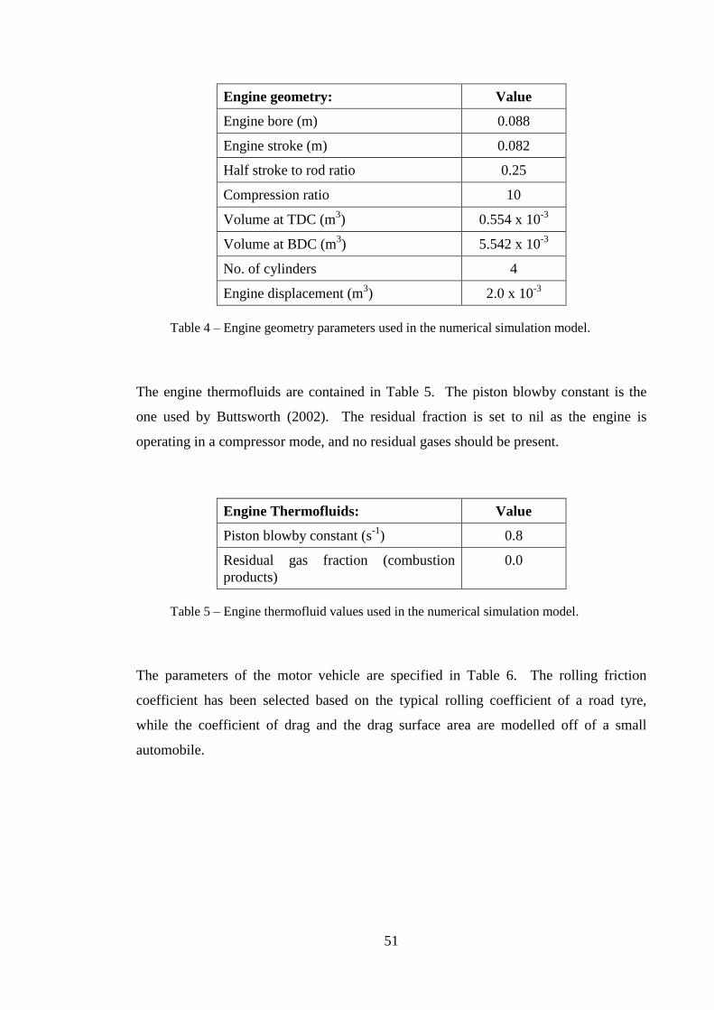
51

Engine geometry: Value

Engine bore (m) 0.088

Engine stroke (m) 0.082

Half stroke to rod ratio 0.25

Compression ratio 10

Volume at TDC (m3) 0.554 x 10

-3

Volume at BDC (m3) 5.542 x 10

-3

No. of cylinders 4

Engine displacement (m3) 2.0 x 10

-3

Table 4 – Engine geometry parameters used in the numerical simulation model.

The engine thermofluids are contained in Table 5. The piston blowby constant is the

one used by Buttsworth (2002). The residual fraction is set to nil as the engine is

operating in a compressor mode, and no residual gases should be present.

Engine Thermofluids: Value

Piston blowby constant (s-1

) 0.8

Residual gas fraction (combustion

products)

0.0

Table 5 – Engine thermofluid values used in the numerical simulation model.

The parameters of the motor vehicle are specified in Table 6. The rolling friction

coefficient has been selected based on the typical rolling coefficient of a road tyre,

while the coefficient of drag and the drag surface area are modelled off of a small

automobile.

52

Vehicle Parameters Value

Mass (kg) 1360

Rolling friction coefficient 0.015

Mechanical Efficiency 0.9

Coefficient of drag 0.3

Drag Surface Area (m2) 2.3

Tire radius (m) 0.3

Table 6 – Vehicle parameters used in the numerical simulation model.

The parameters of the air tank are specified in Table 7. The initial pressure and

temperature are assumed to be at atmospheric pressure and temperature.

Air Tank Parameters Value

Volume (m3) 0.05

Initial pressure (kPa) 101

Initial temperature (K) 300

Table 7 – Air tank parameters used in the numerical simulation model.

3.2.4 Model Losses

The following section outlines how the heat transfer, flow losses and leakage have been

accounted for in the model.

3.2.4.1 Heat Transfer

The heat exchanged between the cylinder walls and piston, and the gas has been

accounted for using the correlation presented by Woschni (1967). The heat transfer is

therefore a function of the gas pressure, gas temperature and engine speed per Equations

3 and 5 (refer to section 2.1.3.2). Although combustion does not take place during the

53

compression cycle, the change in temperature of the cylinder walls over time is not

considered as it is beyond the scope of this project.

3.2.4.2 Flow Losses

Losses associated with the flow through the intake manifold have been considered by

using a lower intake pressure of 90 kPa and a higher intake temperature of 330 K. All

other flow losses such as the pipe acoustics have not been considered due to the

limitations of the model.

3.2.4.3 Leakage

It is assumed that no leakage occurs from the air tank or the system connecting the air

tank to the engine cylinders. Piston blowby has been considered for the compression

and expansion processes, with the constant detailed in Table 5.

Engine Compressor Simulation 3.3

The model will simulate each revolution by splitting the compression cycle into 5 main

functions as shown in Figure 14.

Figure 14 – Diagram of the processes numerically modelled in MATLAB.

Compression Charging Expansion Intake

Air Tank

Storage

54

3.3.1 Compression

At the commencement of the first stroke, the compression process begins. The model

assumes that this process starts at BDC, when all valves are closed and the piston starts

to move upwards into the cylinder and ends when the charge valve opens. The initial

gas conditions for the first iteration have been calculated based on the intake pressure

and temperature and the valve losses. For all subsequent iterations, the state of the gas

is based on the new intake of gas and the expanded residual gas from the previous cycle.

The compression process is controlled by the function ratescomp.m (Appendix C6).

The function returns the derivatives of pressure, temperature, work, heat transfer and

heat leakage, with respect to crank angle. It takes into consideration the heat transfer

and blowby for each change in crank angle, thereby affecting the pressure and

temperature of the gas in the cylinder.

For simplicity purposes, the ratescomp.m function is run for crank angles of -π to 0.

Using the in-built MATLAB function ode45.m, the differential equations returned by

ratescomp.m are integrated to produce the pressure, temperature and work of the gas in

the cylinder for each change in crank angle. The pressure output was then used to

calculate the crank angle at which the charge valve should open.

3.3.2 Charging

The charging process begins when the charging valve opens and finishes at TDC. For

the purposes of this model, it is assumed that this process takes place at constant

pressure (isobaric) and is isothermal.

The model operates on the basis that for every half engine revolution, mass is charged

to the air tank. That is, two cylinders will pump gas into the tank every half revolution

(for a 4 cylinder engine). In order to determine the change in air mass contained within

the air tank (for each revolution), the change of the mass in the cylinder, before and

after the charging take place, was calculated. The steps used for this calculation are:

55

1. Calculate the mass of the gas in the cylinder just before the charge valve opens

using the ideal gas equation. The state of the gas (pressure and temperature) is

given by the compression data output and the volume of the cylinders calculated

at the determined crank angle.

2. Calculate the mass of the gas in the cylinder at TDC (when the charge valve

closes) using the ideal gas equation. The volume at TDC was used, and the

pressure and temperature of the gas when the charge valve opens (as the process

is considered isobaric and adiabatic).

3. The change in mass was calculated by subtracting the mass calculated in step 3

from the mass calculated in step 2. This is the mass of the charge.

3.3.3 Air Tank Storage

The air tank is modelled on the assumption that the tank is adiabatic. The internal

energy of the tank was calculated using the internal energy equation for an ideal gas.

𝑑𝑈 = 𝑚𝑡 ∙ 𝑐𝑣 ∙ 𝑑𝑇 + 𝑇𝑐 ∙ 𝑐𝑣 ∙ 𝑑𝑚 [J] Equation [17]

Where,

𝑚𝑡 is the initial mass in the tank [kg];

𝑐𝑣 is the specific heat at constant volume;

𝑑𝑇 is the change in temperature of the gas in the tank [K];

𝑇𝑐 is the temperature of the charge [K]; and

𝑑𝑚 is the mass of the charge [kg].

This has been simplified further in Equation 18.

𝑑𝑈 = 𝑑𝑚 ∙ 𝑐𝑣 ∙ 𝑑𝑇 [J] Equation [18]

56

Where 𝑑𝑇 [K] is in respect of a temperature reference point, which has been set at the

initial tank temperature.

Once the mass of the charge has been calculated, the new state of the gas within the air

tank can be calculated. The process used to calculate the new state of the gas in the air

tank is:

1. Calculate the initial internal energy of the air tank using Equation 18 and a

temperature reference point of 30 K.

2. Calculate the internal energy of the charge using Equation 18 and a temperature

reference point of 300 K.

3. Calculate the new internal energy of the tank by adding the energies calculated

in step 1 and 2.

4. Calculate the new state of the gas in the air tank.

o The new temperature is calculated by dividing the total energy in step 3,

by the specific energy multiplied by the combined mass of the charge

and the mass of the tank before charging. The reference temperature was

then added back.

𝑇𝑡 =𝑈𝑡+𝑈𝑐

𝑐𝑣∙(𝑚𝑡+𝑚𝑐)+ 𝑇𝑟𝑒𝑓 [K] Equation [19]

o The new pressure of the tank can be calculated using the ideal gas

equation, with the new mass (step 3), the new temperature (step 4) and

the volume of the tank.

This process is contained in the MATLAB file compressor_mode.m in Appendix C2.

3.3.4 Expansion

The expansion process begins at the start of the second stroke, when the charge valve

closes (at TDC) and the piston begins to move back down. The initial conditions of

pressure and temperature are taken from the pressure and temperature of the gas

calculated at the end of the charging process.

57

The expansion process is governed by the function ratesexp.m (Appendix C7). The

function is very similar to the ratescomp.m function, and returns the same derivatives

(pressure, temperature, work, heat transfer and heat leakage) with respect to crank

angle. It takes into consideration the effects of heat transfer and blowby.

The ratesexp.m function is run for crank angles between 0 and π, although the outputs

used are only considered from 0 to the crank angle calculated when the intake valve

opens. Using the function ode45.m once more, the differential equations returned by

ratesexp.m are integrated to produce values of pressure, temperature and work for each

change in crank angle. The pressure output was then used to calculate the crank angle

at which the intake valve should open.

3.3.5 Intake

The intake process occurs when the intake valve opens and draws in fresh air. It is

assumed that the process occurs when the cylinder pressure reaches intake pressure

during the expansion process. The process is modelled assuming the process is isobaric

and isothermal. The output from the process is used to calculate the new initial

conditions before the compression process starts again.

The steps for calculating the new initial conditions are:

1. Determine the gas mass in the cylinder just before the intake valve opens. This

was calculated using the ideal gas equation, with the state of the gas (given by

the expansion data) at the crank angle when the charge valve opens.

2. Determine the air mass in the cylinder resulting from fresh intake. Using the

ideal gas equation, this is calculated using the change in volume between BDC

and at the crank angle when the intake valve opens, and the intake pressure and

temperature for the fresh gas.

3. Find new initial conditions:

a. Calculate new pressure using partial pressures with respect to the mass

fraction of the fresh intake and the residual gas.

58

b. Calculate the new temperature using ideal gas law and the pressure

calculated in step 3a, volume at BDC and the combined mass in steps 1

and 2.

Model Validation 3.4

A number of tests were carried out to ensure that the model was working correctly.

1. Compression and Expansion Processes: The model started as a combustion engine,

simulating the compression, combustion and expansion strokes. Consequently, the

model had to be changed to remove the combustion process. This involved setting

both the equivalence ratio and the residual exhaust fraction to nil. For the purposes

of this test, the piston blowby constant and the heat transfer were removed to

simulate the processes as ideal. The results are shown in Figures 15, 16 and 17.

The figures show that the gas pressure and temperature return to their initial states at

the end of the processes, while no net work is performed on the gas. The figures

therefore illustrate that the processes are adiabatic and reversible as expected.

Figure 15 – Pressure vs crank angle of the gas in the cylinder for the ideal

compression and expansion processes during testing of the model’s validity.

-180 -90 0 90 1800

1

2

3

4

5

6

7

crank angle (degrees ATC)

pre

ssure

(M

Pa)

59

Figure 16 – Temperature vs crank angle of the gas in the cylinder for the ideal

compression and expansion processes during testing of the model’s validity.

Figure 17 – Work performed (for two of the four cylinders) vs crank angle on the

gas in the cylinder for the ideal compression and expansion processes during

testing of the model’s validity.

2. Charging and Intake Processes: The charging and intake processes were added to

the model and the outputs repeated. Again, the heat transfer and piston blowby have

been removed for this test. Figures 18 and 19 demonstrate that the charging and

intake processes are isobaric and isothermal as expected. Furthermore, Figures 18

-180 -90 0 90 1800

500

1000

1500

2000

2500

3000


tem

pera

ture

(K

)

-180 -90 0 90 180-300

-150

0

150

300

450

600


work

(J)

60

and 21 can be compared with ideal compressor Figures 4b and Figures 4a

respectively for their similar shapes. Finally, the net work per cycle is shown in

Figure 20 which illustrates that pumping work has occurred due to the difference in

tank pressure and intake pressure. The results are shown after a 5 second period at

2,000 RPM.

Figure 18 – Pressure of the gas in the cylinder of the ideal compression cycle

during testing of the model validity.

Figure 19 – Temperature of the gas in the cylinder of the ideal compression cycle

during testing of the model validity.

-180 -90 0 90 1800

0.2

0.4

0.6

0.8

1

Crank angle (degrees ATC)

Pre

ssu

re (

MP

a)

Compression

Charging

Expansion

Intake

-180 -90 0 90 180200

300

400

500

600

700

Crank angle (degrees ATC)

Te

mp

era

ture

(K

)

Compression

Charging

Expansion

Intake

61

Figure 20 – Work performed on the gas in the cylinder of the ideal compression

cycle during testing of the model validity.

Figure 21 – PV diagram of the ideal compression cycle during testing of the model

validity.

3. Tank pressure: The pressure in the tank was tested to ensure that the pressure does

not go over the maximum cylinder pressure. Figure 22 shows that the pressure

increasing over time does not exceed the maximum theoretic pressure indicated by

Equation 9.

-180 -90 0 90 180-300

-150

0

150

300


wo

rk (

J)

Compression

Charging

Expansion

Intake

0 1 2 3 4 5 6

x 10-4

0

0.1

0.2

0.3

0.4

0.5

0.6

0.7

0.8

Volume (m3)

Pre

ssu

re (

MP

a)

Compression

Charging

Expansion

Intake

62

Figure 22 – Air tank pressure per engine revolutions compared to the theoretical

maximum pressure for testing the model for validity.

4. Valve opening times: Now that it has been established that the processes are

working correctly, the opening of the charging and intake valves was tested for

appropriateness over a period of 20 seconds. Figure 23 illustrates several key

effects that would be expected:

a. As the air tank pressure increases, the crank angle at which the valves open

also increases.

b. The valve timing approaches TDC for the charging valve and BDC for the

intake valve.

c. Due to diminishing returns, the difference in valve opening times start

higher, and reduce over time as the pressure in the tank approaches

maximum pressure.

0 10 20 30 40 50 600

0.5

1

1.5

2

2.5

time (seconds)

Ta

nk P

ressu

re (

MP

a)

Tank Pressure

Max. Theoretical Pressure

63

Figure 23 – Charging valve and intake valve opening timing as a function of crank

angle over time during testing of the model validity.

Drive Cycle 3.5

For the purposes producing more meaningful results, the performance of the simulation

will take into account a certain number of variable parameters with respect to a drive

cycle. The drive cycle used in this project is the NEDC. The significant considerations

taken from the model include the speed of the vehicle and the rate of deceleration. The

engine speed will be optimised based on these vehicle performance requirements.

The NEDC is a test cycle designed to assess the emission levels for certification

purposes of light duty vehicles in Europe. The NEDC is performed on a chassis

dynamometer under controlled conditions.

The test is made up of two identifiable components. The first is the Urban Driving

Cycle ECE-15 (Figure 24) which is repeated four times. It represents European city

driving and is characterised by low engine load, low engine speed and low exhaust gas

temperature.

0 10 20 30 40 50 60-180

-90

0

90

180

Time (seconds)

Cra

nk A

ng

le

Intake Valve

Charge Valve

64

Figure 24 – Graph of speed over time for the Urban Driving Cycle ECE-15

(DieselNet 2013).

Table 8 shows the breakdown of the speed and timing of the driving cycle. It is

assumed that all acceleration and deceleration is uniform. The total cycle (after

repetition) lasts 780 seconds with a theoretical distance of 3,976 meters and average

speed of 18.35 km/h (DieselNet 2013).

Time (seconds) Speed (km/h)

0-11 0 (idle)

11-15 Acceleration

15-23 15

23-28 Deceleration

28-49 0

49-61 Acceleration

61-85 32

85-96 Deceleration

96-117 0

117-143 Acceleration

143-155 50

155-163 Deceleration

163-176 32

65



188-195 0

Table 8 – Summary of speed, timing and duration for the Urban Driving Cycle

ECE-15.

The second component is the Extra-Urban Driving Cycle (EUDC) which is completed

once after the completion of the ECE-15 repetitions (Figure 25). It represents a more

aggressive and higher speed driving condition with a maximum speed of 120 km/h.

Figure 25 – Graph of speed and time for the Extra-Urban Driving Cycle (DieselNet

2013).

Table 9 (overpage) illustrates the timing and speed of the EUDC. Total duration of the

cycle is 400 seconds with a theoretical distance of 6,955 meters and an average speed of

62.6 km/h (DieselNet 2013).

66


0-20 0 (idle)

20-61 Acceleration

61-111 70


119-188 50


201-251 70


286-316 100


336-346 120


380-400 0

Table 9 – Summary of speed, timing and duration of the Extra-Urban Driving

Cycle (EUDC).

The important performance characteristics that affect this model are the change in

speed, the time during the speed change, and therefore deceleration. These parameters

have been summarised in the Table 10 with their frequency over the drive cycle.

Deceleration

Event

Initial

Speed

(km/h)

Final

Speed

(km/h)

�̅�

(m/s)

Time

(s)

Deceleration

(m/s2)

Frequency

1 15 0 2.08 5 0.833 4

2 32 0 4.44 11 0.808 4

3 50 32 11.39 8 0.625 4

4 32 0 4.44 12 0.741 4

5 70 50 16.67 8 0.694 1

6 120 0 16.67 34 0.617 1

Table 10 – Summary of deceleration events during the NEDC and the frequency of

their occurrence.

67

4 Results and Discussion

Introduction 4.1

The numerical model produced during this research was applied to the NEDC to

calculate the amount of energy that can be recovered over a driving cycle. Using the six

deceleration events identified in the previous section, the engine speed was optimised to

produce an average BMEP that maximised the effect of compression braking, while

minimising the reliance on the friction brakes.

The energy recoverable over these six events was calculated and recorded. Using this

data, inferences have been made about the possible energy savings that compressed gas

KER can achieve. The results were further analysed, drawing conclusions about the

usefulness of the energy and the efficiency of recovering the energy. Finally, the effect

of heating and flow losses were explored with respect to energy recovery, and the

limitations of the model have also been highlighted.

Engine Speed Optimisation 4.2

Optimising the engine speed for each deceleration event was important for two reasons.

Firstly, it was used to ensure that the braking effect due to compression braking was not

in excess of the braking requirements of the driving cycle. Secondly, it was used to

reduce the reliance on the friction brakes and maximise the amount of energy recovered.

Therefore, the optimisation has been completed on the premise of producing a BMEP

that is equivalent to, or slightly under the average BMEP required.

In order to find the average BMEP required, the braking force necessary during each

deceleration event was calculated and the results compiled. This was achieved using

Equations 10 to 13 of the literature review (refer to section 2.3.4), and the values shown

in Tables 6 and 10 of the methodology. The results are shown in Table 11.

68

Event Fi Fd Frf Fb

1 1,133.3 1.8 200.1 931.4

2 1,099.0 8.1 200.1 890.8

3 850.0 53.3 200.1 596.6

4 1,007.4 8.1 200.1 799.2

5 944.4 114.0 200.1 630.3

6 1,333.3 114.0 200.1 1,019.2

Table 11 – Braking force calculated for each deceleration event of the NEDC test

cycle.

The average BMEP was then calculated using Equation 14 and the vehicle parameters

given in Table 6. The average gear ratio used in this equation was calculated using

Equation 20 below.

𝑟𝑔 = 𝑁/ (𝑠

2𝜋𝑟𝑡) Equation [20]

Where, 𝑁 is the number of engine revolutions during deceleration, 𝑠 is the distance [m]

travelled during deceleration, and 𝑟𝑡 is the operating tire radius [m].

From this equation, it can be seen that the average BMEP required is a function of the

engine speed. As the average BMEP produced is also a function of engine speed, trial

and error was used to find the engine speed to the nearest integer that maximised energy

recovery and reduced the reliance on the friction brakes. The results are shown in Table

12 overpage.

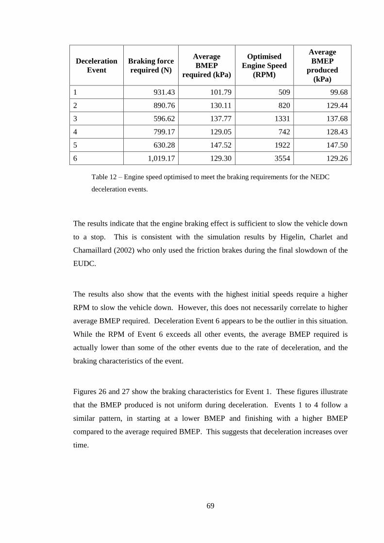
69

Deceleration

Event

Braking force

required (N)

Average

BMEP

required (kPa)

Optimised

Engine Speed

(RPM)

Average

BMEP

produced

(kPa)

1 931.43 101.79 509 99.68

2 890.76 130.11 820 129.44

3 596.62 137.77 1331 137.68

4 799.17 129.05 742 128.43

5 630.28 147.52 1922 147.50

6 1,019.17 129.30 3554 129.26


deceleration events.

The results indicate that the engine braking effect is sufficient to slow the vehicle down

to a stop. This is consistent with the simulation results by Higelin, Charlet and

Chamaillard (2002) who only used the friction brakes during the final slowdown of the

EUDC.

The results also show that the events with the highest initial speeds require a higher

RPM to slow the vehicle down. However, this does not necessarily correlate to higher

average BMEP required. Deceleration Event 6 appears to be the outlier in this situation.

While the RPM of Event 6 exceeds all other events, the average BMEP required is

actually lower than some of the other events due to the rate of deceleration, and the

braking characteristics of the event.

Figures 26 and 27 show the braking characteristics for Event 1. These figures illustrate

that the BMEP produced is not uniform during deceleration. Events 1 to 4 follow a

similar pattern, in starting at a lower BMEP and finishing with a higher BMEP

compared to the average required BMEP. This suggests that deceleration increases over

time.

70


compared to the average BMEP required.


BMEP required.

The exception to this characteristic is in Events 5 and 6. The BMEP produced drops

below the average required BMEP towards the end. This characteristic is especially

pronounced for Event 6 in Figures 28 and 29. The figures illustrate that a peak period

of deceleration occurs in the middle of the deceleration event. On further analysis, the

0 1 2 3 4 50

1

2

3

4

5

Time (s)

BM

EP

(M

Pa

)

Actual BMEP

Required BMEP

0 1 2 3 4 560

70

80

90

100

110

120

130

Time (s)

BM

EP

(kP

a)

Actual BMEP

Required BMEP

71

turning point appears to occur between 110 to 120 revolutions for all events. This

appears to occur because the work recovered by the expansion process begins to

increase relative to the work done during compression and the pumping losses.




average BMEP required.

0 10 20 30 400

50

100

150

200

250

300

Time (s)

BM

EP

(M

Pa

)

Actual BMEP

Required BMEP

0 10 20 30 40100

120

140

160

180

200

Time (s)

BM

EP

(kP

a)

Actual BMEP

Required BMEP

72

The full results of the BMEP produced for Events 1 to 6 are displayed in Figures 35 to

46 in Appendix B2.

Energy Recoverable 4.3

The simulation was run with the engine speed optimised for each braking event. Each

event was run separately, with the tank pressure and temperature at initial conditions.

Therefore, this assumes that the energy is put back into the system after each braking

event. Table 13 shows the energy recovered for each event, multiplied by the frequency

at which the event occurs during the NEDC and the total energy recoverable during the

cycle.

Deceleration Event Energy

Recovered* (kJ) Frequency

Total Energy

Recovered (kJ)

1 5.069 4 20.276

2 28.699 4 114.796

3 35.457 4 141.828

4 28.165 4 112.662

5 53.439 1 53.439

6 131.019 1 131.019

TOTAL 574.020

*Calculated using the change in the internal energy of the air storage tank



73

Figure 30 – Energy change of the tank during the 6 deceleration events of the

NEDC.

Figure 30 shows the change in tank energy over time for the six events. It demonstrates

that the rate of which energy is recovered is based on the speed of the engine. The total

energy recoverable is then a function of time.

Energy Savings 4.4

Using the energy recoverable during the NEDC, inferences can be made about the

potential energy savings. The energy could be used by either using the engine as a

pneumatic motor, using a dedicated pneumatic motor, for supercharging or a

combination like the APA cycle suggested by (Schechter 1999).

To calculate the energy savings, several assumptions have been made.

Energy usable is 80%.

Efficiency of the engine is 30%.

LHV of fuel is 44.4 MJ/kg.

0 10 20 30 400

20

40

60

80

100

120

140

time (seconds)

En

erg

y (

kJ)

Event 1

Event 2

Event 3

Event 4

Event 5

Event 6

74

Density of fuel is 0.745 kg/L.

Therefore, energy savings are estimated using Equation 21:

𝐸𝑠𝑎𝑣𝑖𝑛𝑔𝑠 = 𝐸𝑟𝑒𝑐𝑜𝑣𝑒𝑟𝑒𝑑 ∙𝜂𝑢𝑠𝑢𝑎𝑏𝑙𝑒

𝜂𝑒𝑛𝑔𝑖𝑛𝑒 [J] Equation [21]

= 574020 ∙ 0.80/0.30

= 1530720 J

Furthermore, these savings can be presented in terms of fuel savings per Equation 22:

𝐹𝑠𝑎𝑣𝑖𝑛𝑔𝑠 = 𝐸𝑠𝑎𝑣𝑖𝑛𝑔𝑠 ∙1

𝐿𝐻𝑉𝑓𝑢𝑒𝑙×𝜌𝑓𝑢𝑒𝑙 [L] Equation [22]

= 1530720 ∙1

44.4 ∙ 106 × 0.745

= 0.046 L

As a result, the potential energy savings are 1.5 MJ or 46 x 10-3

L of fuel. At an

estimated 1.143 billion cars in use globally in 2012 (International Organization of

Motor Vehicle Manufacturers n.d.-b), driving on average three times a week for 48

weeks of the year, this translates to a fuel saving of 7.62 GL of fuel savings a year. At a

ratio of 71.92 litres of fuel produced for every barrel of crude oil (U.S. Energy

Information Administration n.d.-b), this represents a saving of 105.9 million barrels of

oil per year, or 0.3% of the estimated 2013 annual consumption.

The effects of shutting down the engine during deceleration and when the vehicle is in

idle have not been considered in this project. The reason for this is that any vehicle can

be adapted to shut down during deceleration. Many vehicles already shut down the

engine when the vehicle would otherwise be idling. However, other researchers such as

Dönitz et al. (2009a) concluded that adding a start/stop capability could increase fuel

savings up to 6%, but has a smaller effect for camless engines.

75

Effect of Losses 4.5

The simulation over the drive cycle performed several more times with an adjustment to

the model parameters to test the effect that losses have on the recovery of energy. The

changes to the model are defined as:

1. Scenario 1: Simulation without heat transfer.

2. Scenario 2: Simulation without blowby.

3. Scenario 3: Simulation with intake at atmospheric conditions optimised for

braking.

The first two scenarios were run without any adjustments to the optimisation of the

engine for a better comparison.

The energy recoverable over the cycle for each scenario is presented in Tables 18 to 21

in Appendix B3. These results have been summarised in Table 14.

Original Scenario 1 Scenario 2 Scenario 3

Total Energy Recoverable (kJ) 574.020 573.116 590.286 519.690

% Energy Change 0% -0.15% 2.8% -9.5%

Table 14 – Summary of energy recoverable using the engine as a compressor with

adjustments to view the changes due to losses.

When no changes are made to the engine speed, the results indicate that the amount of

energy recoverable slightly decreased with no heat exchange, while no leakage

increased the amount of energy recoverable. Therefore, heat exchange increases the

amount energy recoverable while leakage causes losses.

When the engine speed has been optimised for the change of the intake conditions, the

results are not as expected. The amount of energy recoverable would be expected to

increase due greater mass flow rates. However, in this case the energy recoverable has

actually decreased. The reason for this is because the intake conditions at atmospheric

76

pressure and temperature provide a higher BMEP and hence the optimum engine speed

needs to be decreased. As concluded earlier, engine speed affects the rate of energy

recovery. This is shown when comparing Table 15 below with the initial engine speed

optimisation results in Table 12. Consequently, the higher intake temperature with a

lower intake pressure actually produces better results over the NEDC test cycle.

Deceleration

Event

Braking

force

required

(N)

Average

BMEP

required (kPa)

Optimised

Engine Speed

(RPM)

Average

BMEP

produced

(kPa)

1 931.43 101.79 509 100.18

2 890.76 136.43 782 135.50

3 596.62 144.26 1,271 144.22

4 799.17 135.41 707 134.36

5 630.28 154.75 1,827 154.74

6 1,019.17 131.19 3,503 131.19

Table 15 – Optimised engine speed for intake conditions at atmospheric pressure

and temperature.

Other observations 4.6

The following section will discuss the other observations made with respect to

efficiency, tank pressure and tank temperature.

4.6.1 Efficiency of Recovery

The energy recovered for each cycle was compared with the negative IMEP during

compression mode. The results are shown in Figures 31 and 32. Figure 31 shows the

efficiency of each event over time. Based on the slope of the curves, the engine speed

affects the efficiency of recovering the energy. The events with the lower engine speed

have a smaller gradient, peak later and can achieve higher efficiencies. The highest

efficiency observed was 82.74% for Event 4.

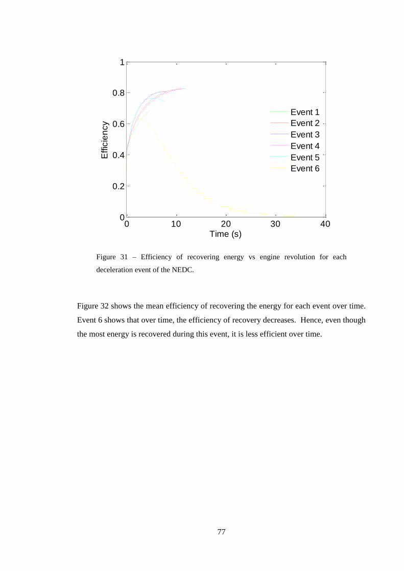
77

Figure 31 – Efficiency of recovering energy vs engine revolution for each

deceleration event of the NEDC.

Figure 32 shows the mean efficiency of recovering the energy for each event over time.

Event 6 shows that over time, the efficiency of recovery decreases. Hence, even though

the most energy is recovered during this event, it is less efficient over time.

0 10 20 30 400

0.2

0.4

0.6

0.8

1

Time (s)

Effic

ien

cy

Event 1

Event 2

Event 3

Event 4

Event 5

Event 6

78

Figure 32 – Mean efficiency of recovering energy vs time for each deceleration

event of the NEDC.

4.6.2 Pressure and Temperature of the Air Tank Over Time

Figures 33 and 34 indicate the pressure and temperature of the air tank over a period of

time for each event. It illustrates that the rate at which the pressure and temperature

increases is related to the speed of the engine. This is to be expected as it is in

alignment with the increase in energy recovered over time shown in Figure 30.

The highest tank pressure recorded was around 2.16 MPa. This is lower than the

theoretical maximum tank pressure of 2.26 MPa. It represents around 96% of the

theoretical maximum pressure. The lowest recorded final pressure was Event 1 with

only 265 kPa or around 12% of the theoretical maximum pressure.

0 10 20 30 400.2

0.3

0.4

0.5

0.6

0.7

0.8

0.9

1

Time (s)

Effic

ien

cy

Event 1

Event 2

Event 3

Event 4

Event 5

Event 6

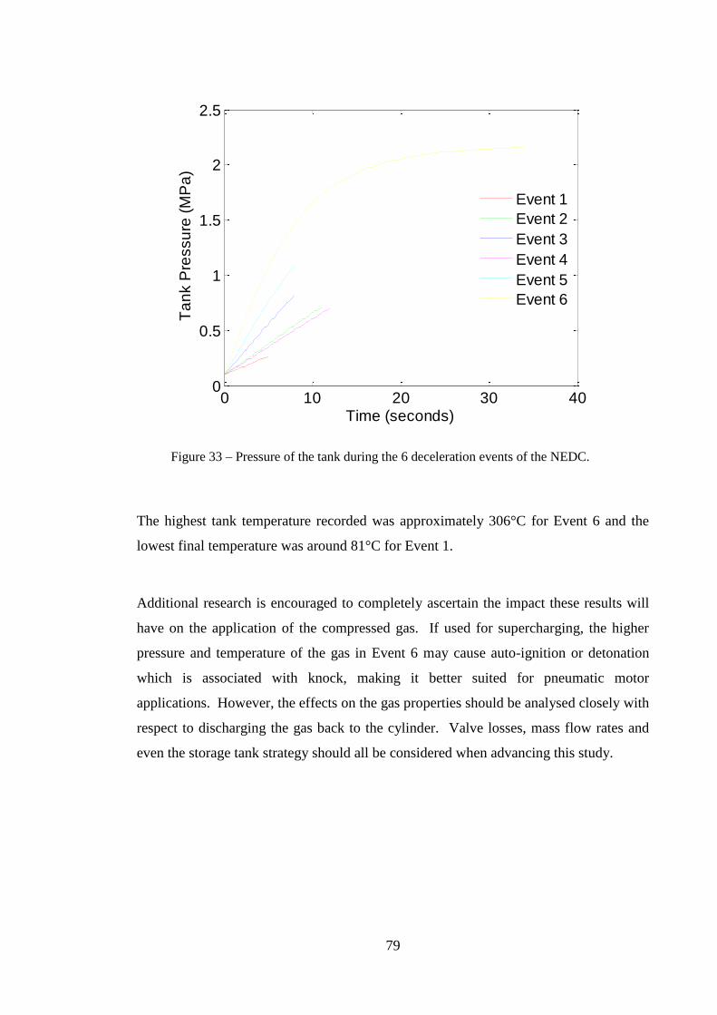
79

Figure 33 – Pressure of the tank during the 6 deceleration events of the NEDC.

The highest tank temperature recorded was approximately 306°C for Event 6 and the

lowest final temperature was around 81°C for Event 1.

Additional research is encouraged to completely ascertain the impact these results will

have on the application of the compressed gas. If used for supercharging, the higher

pressure and temperature of the gas in Event 6 may cause auto-ignition or detonation

which is associated with knock, making it better suited for pneumatic motor

applications. However, the effects on the gas properties should be analysed closely with

respect to discharging the gas back to the cylinder. Valve losses, mass flow rates and

even the storage tank strategy should all be considered when advancing this study.

0 10 20 30 400

0.5

1

1.5

2

2.5

Time (seconds)

Ta

nk P

ressu

re (

MP

a)

Event 1

Event 2

Event 3

Event 4

Event 5

Event 6

80

Figure 34 – Temperature of the tank during the 6 deceleration events of the NEDC.

Limitations 4.7

Of course the model is not without its limitations. Several assumptions have been made

to simplify the model and the simulation of the compression cycle, while there are also

some inherent limitations in the modelling. These are explored in more detail below.

4.7.1 Due to Model Limitations

The opening timing of the charge and intake valves is a limitation in the model. The

step size for the integration parameters used during the compression and expansion

processes was limited to π/180. Consequently, the crank angle at which the valves

opened was calculated at the nearest value of pressure specified for the opening event to

occur. This has two effects. Firstly, it affects the state of the residual gas mixed with

the fresh intake. This is important because the initial pressure, before the compression

process begins, dictates the largest pressure achievable in the tank (as shown in

Equation 9 in section 2.3.1.2) and hence the amount of energy that can be recovered.

0 10 20 30 400

50

100

150

200

250

300

350

Time (s)

Ta

nk T

em

pe

ratu

re (

C)

Event 1

Event 2

Event 3

Event 4

Event 5

Event 6

81

The greatest difference observed between the intake pressure and the pressure at BDC

was 337 Pa greater than and 340 Pa less than intake pressure. However, the average

intake pressure for all events was within 0.1% of the intake pressure.

The second effect occurs during the charging process. The crank angle at which the

charge valve opens is used to calculate the change in the mass of the gas that is

discharged to the air tank. If the charge valve opens too late, then less energy will be

transferred to the tank for that cycle. Hence this will also reduce the efficiency of the

system. In real life however, it would just be a change in work done on the gas which

also affects efficiency.

Similarly, the engine speed optimisation is not exact, and will therefore reduce the

energy recovered due to the assumption that the friction brakes have been used to some

extent.

4.7.2 Due to Assumptions

A restriction relating to the assumptions was that the valve lift was ideal. This

assumption reduces the flow losses that would otherwise occur due to the decrease in

flow area. An increase in pressure drop across the valve was therefore not considered

along with the reduction in mass flow rate. The result is that more energy is recovered

for each cycle in the simulation than what would be expected experimentally.

Another limitation of the model was that the charging and intake processes were treated

as ideal. Therefore, the effects of heat transfer were not considered. However, the heat

transfer during the compression and expansion processes were shown to be negligible, if

not beneficial to some extent. Furthermore, the heat transfer in the air tank was also

neglected. It would be expected that the heat, and therefore energy, would be lost over

time. Therefore, the tank would discharge over time much like batteries in HEVs.

82

Conclusion 4.8

This Results and Discussion section has analysed and discussed the various results

produced from the numerical simulation of an engine operating as a compressor. The

engine was optimised for braking requirements over the NEDC. The energy

recoverable was calculated to be 574 kJ of energy during the braking events over the

entire cycle. Energy savings based on the energy recovered were estimated as 1.5 MJ of

energy for an engine with 30% efficiency and 80% usage of the energy recovered. This

translates to 46 mL of fuel over the cycle.

The effect of the losses was also analysed. These showed that heat transfer actually

recovered a small amount of energy (0.15%), blowby was responsible for a 2.8% energy

loss, and changes in intake conditions which resulted in a decrease of 9.5%. Therefore,

the lower density of the gas assumed initially actually recovered more energy due to the

different BMEP produced and optimised engine speeds.

Other important observations were made about the data. The maximum observed

efficiency was around 83% for energy recovered for a single cycle and 72.76% for the

overall efficiency during a deceleration event. Hence, a regenerative efficiency of

58.2 % is calculated with the assumption of 80% usage of the recovered energy. The

maximum tank pressure and temperature recorded was 2.16 MPa and 306°C

respectively.

Finally, the limitations of the model were discussed with respect to the possible effects

these limitations have had on the results.

83

5 Conclusions

Introduction 5.1

Fuel consumption and sustainability are major drivers influencing regenerative braking

technologies. This is illustrated by the number of manufacturers now exploring and

implementing technologies to recover energy. Other manufactures such as Tesla

Motors are also focusing on a purely electric vehicle alternative. This project

undertaken has considered one of these technologies still in its infancy; the concept of

using the engine as a compressor to recover energy during braking conditions.

This project has discussed the two current kinetic energy recovery technologies: HEV

and Flywheels. The advantages and disadvantages of each technology have been

highlighted for comparison with the concept in the Project Background. The ability to

implement the concept and use an IC engine as a compressor was shown as promising

during the literature review, with several uses for the compressed gas established.

A numerical simulation was undertaken of an engine operating as a compressor during

the deceleration phases of the NEDC. The energy calculated as recoverable during the

modelling and simulation process could potentially have an impact on reducing fuel

consumption and improving the overall efficiency of a vehicle. Although the energy

savings were relatively small, improvements in the technology could make it a more

viable solution.

Viability of the Concept 5.2

This section concludes on the viability of the concept, considering the two main

technologies used for regenerative braking, the ability to use an IC engine as a

compressor, and the possible applications for the compressed gas.

84

5.2.1 Comparison with Current Technologies

The Project Background introduced HEV and Flywheel regenerative braking. The

literature revealed several advantages and disadvantages associated with each

technology.

HEVs appear to have the advantage as a storage medium. Both batteries and capacitors

can store energy for longer periods of time. Flywheels tend to self-discharge at much

quicker rates due to friction, while compressed gas will lose energy through heat.

Although, compressed gas with lower heats are more suitable for supercharging to avoid

the effects of engine knock.

When it comes to efficiency, the literature suggests that Flywheels may have the

advantage. HEVs need to convert energy from kinetic energy, to electric energy, and

finally chemical energy, and then back again to use the energy. Body & Brockbank

(2009) (cited in Boretti 2010) claims an overall charge, discharge efficiency of more

than 70% during a full regenerative cycle in stop start traffic. In comparison to the

results of the simulation conducted in this project, the regenerative efficiency is 58.2%

after the assumption that 80% of the energy recovered could be used. This compares

with a maximum overall efficiency of 33% calculated by Trajkovic et al. (2007).

However, the experimental results of Dönitz et al. (2009b) demonstrate regenerative

efficiencies of only 13.8%. This is quite low compared to HEVs which can have

efficiencies of about 60% (Dönitz et al. 2009b).

Other researchers have shown that compressed gas technology can be competitive when

it comes to fuel savings. Early simulations performed by Higelin, Charlet and

Chamaillard (2002) suggested fuel savings of around 15% over the NEDC test cycle.

However, Dönitz et al. (2009a) concluded that fuel savings of 34% were achievable

over the NEDC by using a downsized camless engine with pneumatic hybridization.

This can be compared with the 18% demonstrated by Flybrid Automotive Limited

(2014) for their Flywheel technology over the NEDC test cycle. Furthermore, Volvo

Car Group (2014) claim fuel consumption reductions of 25% for their joint tests with

Flybrid Automotive. Meanwhile, Toyota Motor Corporation Australia Ltd (n.d.) claim

85

ambitious fuel savings of up to 50% for their Prius model compared to similar size

vehicles. However, it remains unclear how they have calculated and arrived at these

impressive results.

The literature reviewed as part of this project suggests that compressed gas technology

also has the advantage of reduced weight, which affects vehicle performance and fuel

consumption. The additional weight for a pressure vessel, VVT and other hydraulic

components is estimated to be just 25 kg (Dönitz et al. 2009a). If the energy is used for

supercharging, this will also allow for downsizing of the engine, which can reduce the

overall mass by more the 25kg (Dönitz et al. 2009b). This is substantially less than a

HEV such as the Prius, which has battery mass of 53.3 kg according to Berman (2008).

This is without even considering the extra components such as the electric motor to

deliver power back to the drivetrain.

All technologies have a safety factor. Compressed gas requires pressure vessels that

must be maintained. HEVs obviously add electricity to the equation which presents

new dynamics to safety in crashes. They also have chemical components that can be

toxic. Finally, Flywheels store a high amount of kinetic energy in a confined volume.

Failure of such a device requires the housing to be manufactured to withstand the

energy in the event of failure.

5.2.2 Ability to Use the Engine as a Compressor

The literature reviewed in this study reveals that the ability to use the engine as a

compressor is fairly established. It appears that the concept requires very few

additional components or modifications.

The ability to implement the concept hinges on the use of variable valve timing. This

solution provides the engine with the ability to not just operate in compression mode,

but also as a pneumatic engine. Furthermore, it provides benefits when the engine is

operating conventionally. Dönitz et al. (2009a) concluded that it could improve fuel

consumption by 8% alone without any other improvements.

86

Modifying the cylinder head was also a prominent feature in the literature. Although

many configurations were witnessed, an addition of a single charging valve seemed to

be the most widely accepted solution.

Finally, a storage tank would be required to store the compressed gas. The size of the

tank is dependent upon trade-off between the cost, optimal energy recoverable and the

space constraints. With this component, also comes the need for safety considerations,

including the need to ensure that tank temperature and pressure do not exceed design

specifications.

5.2.3 Applications of the Compressed Gas

The applications considered in this project while limited, were very applicable to

reducing fuel consumption. The two main uses considered were supercharging and

pneumatic engines. Researchers have shown that both applications have their benefits.

Dönitz et al. (2009a) concluded that supercharging allows for downsizing of the engine

resulting in greater fuel savings. Using the compressed gas to supercharge also doesn’t

suffer from lag associated with turbochargers or losses with superchargers.

The alternate application is to use either the engine in a pneumatic motor mode, or using

a dedicated pneumatic motor. Using the engine as a pneumatic motor reduces the need

for extra componentry, therefore reducing overall vehicle mass and subsequently fuel

consumption. However, dedicated pneumatic motors used in parallel with the engine

also provide the ability to recover heat by recycling the exhaust gas, as shown by Huang

and Tzeng (2005).

Conclusion 5.3

Overall, the concept of using compressed gas to recover kinetic energy appears to be

viable. With additional components and modifications, an engine can be used as a

compressor. The technology has many benefits and potential to improve with time.

87

However, current performance in experimental results appear inferior (to some degree)

than the performance of the other two prominent technologies.

Whether or not it could compete with HEVs in the market, is still currently unclear.

The research suggests that more effort needs to be invested in producing experimental

results and subsequently optimising the system to improve overall performance.

Further Work 5.4

Due to the timeframe constraints associated with the development of this study, many

factors have been identified as needing to be either considered, or considered in more

depth. In continuance of this project, the simulation produced needs to fully consider

the effects of heat transfer, leakage, and flow losses through the intake system and

across the valves. While these factors have already been considered to some extent, the

considerations in the model are relatively limited and should be investigated in more

depth in order to provide more meaningful comparisons with any eventual experimental

setup. Furthermore, the application of the compressed gas needs to be considered in

the simulation and the associated fuel savings and regenerative efficiency over the

whole cycle.

Boretti (2010)

88

6 References

Asmus, TW 1982, 'Valve Events and Engine Operation', SAE Paper 820749.

Berman, B 2008, The Hybrid Car Battery: A Definitive Guide, Hybrid Cars, viewed 27 October 2014, <http://www.hybridcars.com/hybrid-car-battery/>.

Boretti, A 2010, 'Comparison of fuel economies of high efficiency diesel and hydrogen engines powering a compact car with a flywheel based kinetic energy recovery systems', International Journal of Hydrogen Energy, vol. 35, no. 16, pp. 8417-24.

Buttsworth, D 2002, Spark Ignition Internal Combustion Engine Modelling using Matlab, Faculty of Engineering & Surveying, University of Southern Queensland.

Ceviz, M 2007, 'Intake plenum volume and its influence on the engine performance, cyclic variability and emissions', Energy Conversion and Management, vol. 48, no. 3, pp. 961-6.

Ceviz, M & Akin, M 2010, 'Design of a new SI engine intake manifold with variable length plenum', Energy Conversion and Management, vol. 51, no. 11, pp. 2239-44.

DieselNet 2013, Emission Test Cycles: ECE15 + EUDC/NEDC, United Nations Environment Program, viewed 11 October 2014, <https://www.dieselnet.com/standards/cycles/ece_eudc.php>.

Dönitz, C, Vasile, I, Onder, C & Guzzella, L 2009a, 'Dynamic programming for hybrid pneumatic vehicles', in American Control Conference 2009, Hyatt Regency Riverfront, St. Louis, MO, USA, pp. 3956-63.

Dönitz, C, Vasile, I, Onder, C & Guzzella, L 2009b, 'Realizing a Concept for High Efficiency and Excellent Driveability: The Downsized and Supercharged Hybrid Pneumatic Engine', SAE Paper 2009-01-1326.

Elkady, M, Elmarakbi, A, Knapton, D, Saleh, M, Abdelhameed, M & Bawady, A 2013, 'Theoretical and Experimental Analysis of Electromagnetic Variable Valve Timing Control Systems for Improvement of Spark Ignition Engine Performance', Advances in Automobile Engineering, viewed 27 October 2014, <http://omicsgroup.org/>.

Ferguson, CR 1986, Internal Combustion Engines, Applied Thermosciences, John Wiley and Sons, New York.

89

Flybrid Automotive Limited 2014, Road Car Systems, Flybrid Automotive Limited, viewed 18 October 2014, <http://www.flybridsystems.com/Roadcar.html>.

Fontana, G & Galloni, E 2009, 'Variable valve timing for fuel economy improvement in a small spark-ignition engine', Applied Energy, vol. 86, no. 1, pp. 96-105.

Fuhs, A 2009, Hybrid vehicles and the future of personal transportation, CRC Press, Boca Raton.

Gordon, S & McBride, BJ 1971, Computer Program for Calculation of Complex Chemical Equilibrium Composition, Rocket Performance, Incident and Reflected Shocks, and Chapman-Jouguet Detonations, NASA publication SP-273.

Hanlon, P 2001, Compressor handbook, McGraw-Hill, New York.

Heywood, J 1988, Internal combustion engine fundamentals, McGraw-Hill, New York.

Higelin, P, Charlet, A & Chamaillard, Y 2002, 'Thermodynamic Simulation of a Hybrid Pneumatic-Combustion Engine Concept', International journal of applied thermodynamics, vol. 5, no. 1, pp. 1-11.

Huang, KD & Tzeng, S-C 2005, 'Development of a hybrid pneumatic-power vehicle', Applied Energy, vol. 80, no. 1, pp. 47-59.

Huang, KD, Tzeng, S-C, Ma, W-P & Chang, W-C 2005, 'Hybrid pneumatic-power system which recycles exhaust gas of an internal-combustion engine', Applied Energy, 10//, pp. 117-32.

International Organization of Motor Vehicle Manufacturers n.d.-a, International Energy Statistics International Organization of Motor Vehicle Manufacturers, viewed 2 June 2014, <http://www.eia.gov/cfapps/ipdbproject/IEDIndex3.cfm?tid=5&pid=57&aid=6>.

International Organization of Motor Vehicle Manufacturers n.d.-b, 2013 Production Statistics, International Organization of Motor Vehicle Manufacturers, viewed June 2, <http://www.oica.net/category/production-statistics/>.

Kang, H, Tai, C, Smith, E, Wang, X, Tsao, T-C, Stewart, J & Blumberg, P 2008, 'Demonstration of Air-Power-Assist (APA) Engine Technology for Clean Combustion and Direct Energy Recovery in Heavy Duty Application', SAE Paper 2008-01-1197.

90

Motor Trend Magazine 2014a, Flywheel KERS: Flywheel Module, Motor Trend Magazine, viewed 18 October 2014, <http://wot.motortrend.com/volvo-experimenting-flywheel-hybrid-claims-reduce-fuel-consumption-20-percent-82025.html/volvo-flywheel-kers-diagram-1/>.

Motor Trend Magazine 2014b, Flywheel KERS: System Layout, Motor Trend Magazine, viewed 18 October 2014, <http://wot.motortrend.com/volvo-experimenting-flywheel-hybrid-claims-reduce-fuel-consumption-20-percent-82025.html/volvo-flywheel-kers-diagram-2/>.

Organization of the Petroleum Exporting Countries 2013, 2013 World Oil Outlook, Organization of the Petroleum Exporting Countries, <http://www.opec.org/opec_web/static_files_project/media/downloads/publications/WOO_2013.pdf>.

Pritchard, P 2011, Fox and McDonald's Introduction to Fluid Mechanics, 8th edn, John Wiley & Sons, Inc., Hoboken, N.J.

Pulkrabek, W 1997, Engineering fundamentals of the internal combustion engine, Prentice Hall, Upper Saddle River, N.J.

Schechter, M 1999, New Cycles for Automobile Engines, SAE Paper 1999-01-0623.

Tai, C, Tsao, T-C, Levin, M, Barta, G & Schechter, M 2003, 'Using Camless Valvetrain for Air Hybrid Optimization', SAE Paper 2003-01-0038.

Toyota Motor Corporation Australia Ltd n.d., Hybrid Performance, viewed 20 October 2014, <http://www.toyota.com.au/prius/features/hybrid-performance>.

Trajkovic, S, Tunestål, P, Johansson, B, Carlson, U & Höglund, A 2007, 'Introductory Study of Variable Valve Actuation for Pneumatic Hybridization', SAE Paper 2007-01-0288.

U.S. Energy Information Administration n.d.-a, International Energy Statistics, U.S. Energy Information Administration, viewed 31 May 2014, <http://www.eia.gov/>.

U.S. Energy Information Administration n.d.-b, Frequently Asked Questions, U.S. Energy Information Administration, viewed 20 October 2014, <http://www.eia.gov/tools/faqs/faq.cfm?id=24&t=10>.

U.S. Government n.d.-a, Where the Energy Goes: Gasoline Vehicles, U.S. Government, viewed 2 June 2014, <http://www.fueleconomy.gov/feg/atv.shtml>.

91

U.S. Government n.d.-b, How Hybrids Work, U.S. Government, viewed 20 October 2014, <http://www.fueleconomy.gov/feg/hybridtech.shtml>.

Volvo Car Group 2014, Volvo Car Group and Flybrid Conduct UK Testing of Flywheel KERS Technology, Volvo Car Group, viewed 18 October 2014, <https://www.media.volvocars.com/uk/en-gb/media/pressreleases/141626/volvo-car-group-and-flybrid-conduct-uk-testing-of-flywheel-kers-technology>.

Woschni, G 1967, 'A Universally Applicable Equation for the Instantaneous Heat Transfer Coefficient in the Internal Combustion Engine', SAE Paper 670931.

92

Appendix A – Project Specification


FACULTY OF HEALTH, ENGINEERING AND SCIENCES

ENG4111/ENG41112

PROJECT SPECIFICATION

FOR: Rick Kruger

TOPIC: KINETIC ENERGY RECOVERY SYSTEM USING

COMPRESSED GAS

SUPERVISOR: Dr Ray Malpress

ENROLMENT: ENG4111 – S1 2014

ENG4112 – S2 2014

PROJECT AIM: This project seeks to investigate the potential recovery of kinetic

energy using compressed gas of a moving motor vehicle under

braking, considering the amount of energy recoverable and the

potential uses of that energy.

PROGRAMME: Version 1, 17 March 2014

1. Research the background information relating to automotive Kinetic Energy

Recovery Systems and compression systems.

2. Critically evaluate current Kinetic Energy Recovery Systems and their use.

3. Investigate, analyse and evaluate alternate uses of compressed gas in automotive

systems.

4. Design a model of a Kinetic Energy Recovery System using compressed gas

(Matlab).

5. Calculate expected energy recovery and compare with current systems.

6. Analyse and conclude on practicality, efficiency/fuel savings, cost and limitations.

7. Submit an academic dissertation on the research.

As time permits:

8. Design and build a small working model of the system.

9. Collect output data, analyse and compare data to the theoretical model calculations.

10. Investigate potential improvements.

AGREED:

__________ (Student) __________ (Supervisor) __________ (Examiner)

__/__/____ __/__/____ __/__/____

93

Appendix B1 – Results: Optimised Braking Speed

Deceleration

Event

Braking

force

required

(N)

Average

BMEP

required (kPa)

Optimised

Engine Speed

(RPM)

Average

BMEP

produced

(kPa)

1 931.43 101.79 509 99.68

2 890.76 130.11 820 129.44

3 596.62 137.77 1331 137.68

4 799.17 129.05 742 128.43

5 630.28 147.52 1922 147.50

6 1,019.17 129.30 3554 129.26



Deceleration

Event

Braking

force

required

(N)

Average

BMEP

required (kPa)

Optimised

Engine Speed

(RPM)

Average

BMEP

produced

(kPa)

1 931.43 101.79 509 100.18

2 890.76 136.43 782 135.50

3 596.62 144.26 1,271 144.22

4 799.17 135.41 707 134.36

5 630.28 154.75 1,827 154.74

6 1,019.17 131.19 3,503 131.19

Table 17 – Optimised engine speed for intake conditions at atmospheric pressure

and temperature.

94

Appendix B2 – Results: Required BMEP vs Actual BMEP




BMEP required.

0 1 2 3 4 50

1

2

3

4

5

Time (s)

BM

EP

(M

Pa

)

Actual BMEP

Required BMEP

0 1 2 3 4 560

70

80

90

100

110

120

130

Time (s)

BM

EP

(kP

a)

Actual BMEP

Required BMEP

95





0 2 4 6 8 10 120

5

10

15

20

Time (s)

BM

EP

(M

Pa

)

Actual BMEP

Required BMEP

0 2 4 6 8 10 1260

80

100

120

140

160

Time (s)

BM

EP

(kP

a)

Actual BMEP

Required BMEP

96





0 2 4 6 80

5

10

15

20

25

Time (s)

BM

EP

(M

Pa

)

Actual BMEP

Required BMEP

0 2 4 6 870

80

90

100

110

120

130

140

150

Time (s)

BM

EP

(kP

a)

Actual BMEP

Required BMEP

97





0 2 4 6 8 10 120

5

10

15

20

Time (s)

BM

EP

(M

Pa

)

Actual BMEP

Required BMEP

0 2 4 6 8 10 1260

80

100

120

140

160

Time (s)

BM

EP

(kP

a)

Actual BMEP

Required BMEP

98




average BMEP required

0 2 4 6 80

5

10

15

20

25

30

35

40

Time (s)

BM

EP

(M

Pa

)

Actual BMEP

Required BMEP

0 2 4 6 880

90

100

110

120

130

140

150

160

Time (s)

BM

EP

(kP

a)

Actual BMEP

Required BMEP

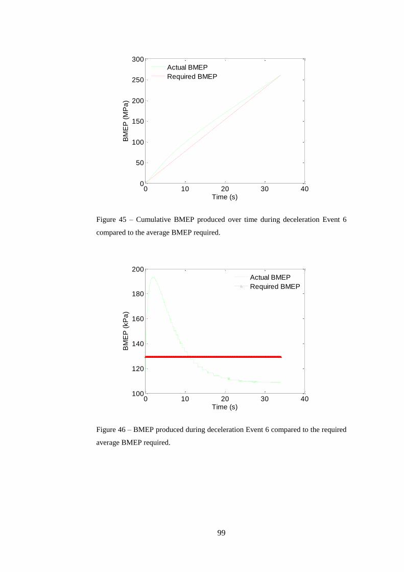
99





0 10 20 30 400

50

100

150

200

250

300

Time (s)

BM

EP

(M

Pa

)

Actual BMEP

Required BMEP

0 10 20 30 40100

120

140

160

180

200

Time (s)

BM

EP

(kP

a)

Actual BMEP

Required BMEP

100

Appendix B3 – Results: Energy Recovered

Deceleration Event Energy Recovered

(kJ) Frequency

Total Energy

Recovered (kJ)

1 5.069 4 20.276

2 28.699 4 114.796

3 35.457 4 141.828

4 28.165 4 112.662

5 53.439 1 53.439

6 131.019 1 131.019

TOTAL 574.020




(kJ) Frequency

Total Energy

Recovered (kJ)

1 5.059 4 20.236

2 28.621 4 114.483

3 35.371 4 141.482

4 28.089 4 112.354

5 53.332 1 53.332

6 131.229 1 131.229

TOTAL 573.116

Table 19 – Energy recovered for each deceleration event without heat transfer.

101


(kJ) Frequency

Total Energy

Recovered (kJ)

1 5.262 4 21.047

2 29.700 4 118.802

3 36.237 4 144.949

4 29.212 4 116.848

5 54.305 1 54.305

6 134.335 1 134.335

TOTAL 590.286

Table 20 – Energy recovered for each deceleration event without blowby.


(kJ) Frequency

Total Energy

Recovered (kJ)

1 3.532 4 14.129

2 24.740 4 98.958

3 31.389 4 125.554

4 24.159 4 96.636

5 49.352 1 49.352

6 135.061 1 135.061

TOTAL 519.690

Table 21 – Energy recovered for each deceleration event without intake flow

losses.

102

Appendix C1 – Airdata.m

function A=airdata(scheme);

%

% A=airdata(scheme)

%

% Routine to specify the thermodynamic properties of air and

% combustion products.

% Data taken from:

% 1. Gordon, S., and McBride, B. J., 1971, "Computer Program for

% Calculation of Complex Chemical Equilibrium Composition, Rocket

% Performance, Incident and Reflected Shocks, and Chapman-Jouguet

% Detonations," NASA SP-273. As reported in Ferguson, C. R., 1986,

% "Internal Combustion Engines", Wiley.

% 2. Kee, R. J., et al., 1991, "The Chemkin Thermodynamic Data Base",

% Sandia Report, SAND87-8215B. As reported in

% Turns, S. R., 1996, "An Introduction to Combustion:

% Concepts and Applications", McGraw-Hill.

% ********************************************************************

% input:

% scheme switch:

% 'GMcB_low' - Gordon and McBride 300 < T < 1000 K

% 'GMcB_hi' - Gordon and McBride 1000 < T < 5000 K

% 'Chemkin_low' - Chemkin 300 < T < 1000 K

% 'Chemkin_hi' - Chemkin 1000 < T < 5000 K

% output:

% A - matrix of polynomial coefficients for cp/R, h/RT, and s/R

% of the form h/RT=a1+a2*T/2+a3*T^2/3+a4*T^3/4+a5*T^4/5*a6/T (for

% example) where T is expressed in K

% columns 1 to 7 are coefficients a1 to a7, and

% rows 1 to 10 are species CO2 H2O N2 O2 CO H2 H O OH and NO

% ********************************************************************

switch scheme

case 'GMcB_low'

A=[ 0.24007797E+01 0.87350957E-02 -0.66070878E-05 0.20021861E-08

...

0.63274039E-15 -0.48377527E+05 0.96951457E+01

0.40701275E+01 -0.11084499E-02 0.41521180E-05 -0.29637404E-08

...

0.80702103E-12 -0.30279722E+05 -0.32270046E+00

103

0.36748261E+01 -0.12081500E-02 0.23240102E-05 -0.63217559E-09

...

-0.22577253E-12 -0.10611588E+04 0.23580424E+01

0.36255985E+01 -0.18782184E-02 0.70554544E-05 -0.67635137E-08

...

0.21555993E-11 -0.10475226E+04 0.43052778E+01

0.37100928E+01 -0.16190964E-02 0.36923594E-05 -0.20319674E-08

...

0.23953344E-12 -0.14356310E+05 0.29555350E+01

0.30574451E+01 0.26765200E-02 -0.58099162E-05 0.55210391E-08

...

-0.18122739E-11 -0.98890474E+03 -0.22997056E+01

0.25000000E+01 0.00000000E+00 0.00000000E+00 0.00000000E+00

...

0.00000000E+00 0.25471627E+05 -0.46011762E+00

0.29464287E+01 -0.16381665E-02 0.24210316E-05 -0.16028432E-08

...

0.38906964E-12 0.29147644E+05 0.29639949E+01

0.38375943E+01 -0.10778858E-02 0.96830378E-06 0.18713972E-09

...

-0.22571094E-12 0.36412823E+04 0.49370009E+00

0.40459521E+01 -0.34181783E-02 0.79819190E-05 -0.61139316E-08

...

0.15919076E-11 0.97453934E+04 0.29974988E+01];

case 'GMcB_hi'

A=[ 0.44608041E+01 0.30981719E-02 -0.12392571E-05 0.22741325E-09

...

-0.15525954E-13 -0.48961442E+05 -0.98635982E+00

0.27167633E+01 0.29451374E-02 -0.80224374E-06 0.10226682E-09

...

-0.48472145E-14 -0.29905826E+05 0.66305671E+01

0.28963194E+01 0.15154866E-02 -0.57235277E-06 0.99807393E-10

...

-0.65223555E-14 -0.90586184E+03 0.61615148E+01

0.36219535E+01 0.73618264E-03 -0.19652228E-06 0.36201558E-10

...

-0.28945627E-14 -0.12019825E+04 0.36150960E+01

0.29840696E+01 0.14891390E-02 -0.57899684E-06 0.10364577E-09

...

-0.69353550E-14 -0.14245228E+05 0.63479156E+01

104

0.31001901E+01 0.51119464E-03 0.52644210E-07 -0.34909973E-10

...

0.36945345E-14 -0.87738042E+03 -0.19629421E+01

0.25000000E+01 0.00000000E+00 0.00000000E+00 0.00000000E+00

...

0.00000000E+00 0.25471627E+05 -0.46011763E+00

0.25420596E+01 -0.27550619E-04 -0.31028033E-08 0.45510674E-11

...

-0.43680515E-15 0.29230803E+05 0.49203080E+01

0.29106427E+01 0.95931650E-03 -0.19441702E-06 0.13756646E-10

...

0.14224542E-15 0.39353815E+04 0.54423445E+01

0.31890000E+01 0.13382281E-02 -0.52899318E-06 0.95919332E-10

...

-0.64847932E-14 0.98283290E+04 0.67458126E+01];

case 'Chemkin_low'

A=[ 0.02275724E+02 0.09922072E-01 -0.10409113E-04 0.06866686E-07

...

-0.02117280E-10 -0.04837314E+06 0.10188488E+02

0.03386842E+02 0.03474982E-01 -0.06354696E-04 0.06968581E-07

...

-0.02506588E-10 -0.03020811E+06 0.02590232E+02

0.03298677E+02 0.14082404E-02 -0.03963222E-04 0.05641515E-07

...

-0.02444854E-10 -0.10208999E+04 0.03950372E+02

0.03212936E+02 0.11274864E-02 -0.05756150E-05 0.13138773E-08

...

-0.08768554E-11 -0.10052490E+04 0.06034737E+02

0.03262451E+02 0.15119409E-02 -0.03881755E-04 0.05581944E-07

...

-0.02474951E-10 -0.14310539E+05 0.04848897E+02

0.03298124E+02 0.08249441E-02 -0.08143015E-05 -0.09475434E-09

...

0.04134872E-11 -0.10125209E+04 -0.03294094E+02

0.02500000E+02 0.00000000E+00 0.00000000E+00 0.00000000E+00

...

0.00000000E+00 0.02547162E+06 -0.04601176E+01

0.02946428E+02 -0.16381665E-02 0.02421031E-04 -0.16028431E-08

...

0.03890696E-11 0.02914764E+06 0.02963995E+02

105

0.03637266E+02 0.01850910E-02 -0.16761646E-05 0.02387202E-07

...

-0.08431442E-11 0.03606781E+05 0.13588605E+01

0.03376541E+02 0.12530634E-02 -0.03302750E-04 0.05217810E-07

...

-0.02446262E-10 0.09817961E+05 0.05829590E+02];

case 'Chemkin_hi'

A=[ 0.04453623E+02 0.03140168E-01 -0.12784105E-05 0.02393996E-08

...

-0.16690333E-13 -0.04896696E+06 -0.09553959E+01

0.02672145E+02 0.03056293E-01 -0.08730260E-05 0.12009964E-09

...

-0.06391618E-13 -0.02989921E+06 0.06862817E+02

0.02926640E+02 0.14879768E-02 -0.05684760E-05 0.10097038E-09

...

-0.06753351E-13 -0.09227977E+04 0.05980528E+02

0.03697578E+02 0.06135197E-02 -0.12588420E-06 0.01775281E-09

...

-0.11364354E-14 -0.12339301E+04 0.03189165E+02

0.03025078E+02 0.14426885E-02 -0.05630827E-05 0.10185813E-09

...

-0.06910951E-13 -0.14268350E+05 0.06108217E+02

0.02991423E+02 0.07000644E-02 -0.05633828E-06 -0.09231578E-10

...

0.15827519E-14 -0.08350340E+04 -0.13551101E+01

0.02500000E+02 0.00000000E+00 0.00000000E+00 0.00000000E+00

...

0.00000000E+00 0.02547162E+06 -0.04601176E+01

0.02542059E+02 -0.02755061E-03 -0.03102803E-07 0.04551067E-10

...

-0.04368051E-14 0.02923080E+06 0.04920308E+02

0.02882730E+02 0.10139743E-02 -0.02276877E-05 0.02174683E-09

...

-0.05126305E-14 0.03886888E+05 0.05595712E+02

0.03245435E+02 0.12691383E-02 -0.05015890E-05 0.09169283E-09

...

-0.06275419E-13 0.09800840E+05 0.06417293E+02];

end

106

Appendix C2 – Compressor_mode.m

% compressor_mode.m % % Script file to determine the performance of a fuel inducted engine % operating as a compressor. % ******************************************************************** % Originally based on a file to determine the performance of a fuel % inducted engine (user-specified) arbitrary heat release profile as a % function of crank angle. % ******************************************************************** % input: % enginedata.m - this is another script file that defines all of the % relevant engine parameters and operating conditions. % output: % output.mat - this file contains all of the variables. % ********************************************************************

clear timestart=cputime;

global b stroke eps r Cblowby f fueltype airscheme phi ... thetas thetab omega ... heattransferlaw hcu hcb ... Tw theta1 Vtdc Vbdc mass1 ... p1 T1 V1 RPM thetac cylinders ... Vd Cv Rair Tref Pa Ta k g rho r ... stoptime speedkm endspeedkm

% load the engine parameters and initial conditions enginedata

% Set vehicle parameters stoptime=8; % time to complete stop speedkm(1)=70; % initial speed of the MV in km/h endspeedkm=50; % ending speed MVmass=1360; % mass of the MV in kg %******************************************************************** speedm(1)=speedkm*1000/3600; % initial speed of the MV in m/s endspeedm=endspeedkm*1000/3600; % ending speed Vmean=(speedm(1)+endspeedm)/2; % mean velocity MVKE(1)=0.5*MVmass*speedm(1)^2; % initial KE of the vehicle decel=(speedm(1)-endspeedm)/stoptime; % deceleration distance=speedm(1)*stoptime-0.5*decel*stoptime^2; % braking distance revolutions=round(RPM/60*stoptime)+1; % total engine revolutions

% Calculate braking requirements f=0.015; % rolling friction coefficient Cd=0.3; % coefficient of drag A=2.3; % total surface area in contact with the air (m^2) rt=0.3; % tire radius nt=0.9; % mechanical efficiency of the transmission and driveline rg=revolutions/(distance/(pi*rt*2)); % average gear ratio (RPM:tire) Fi=MVmass*decel; % inertial force Frf=MVmass*g*f; % rolling friction force Fd=Cd*0.5*rho*(Vmean^2)*A; % drag force Fb=Fi-Frf-Fd; % braking force required BMEPR=Fb*2*pi*rt*nt/(rg*Vd); % Average required BMEP per rev

107

% Set intake pressure and temperature Tintake=T1; Pintake=p1;

% Set initial tank parameters Ptank(1)=Pa; Ttank(1)=Ta; Tref=Ttank(1); Vtank=0.05; Mtank(1)=Ptank(1)*Vtank/(Ttank(1)*Rair); UTank(1)=Mtank(1)*Cv*(Ttank(1)-Tref); Ptankmax=Pintake*r^k;

% Set initial values time(1)=0; p23=p1; T23=T1; p14=p1; T14=T1; Ucharge14(1)=0; Ucharge23(1)=0; UCHARGE(1)=0; UCHARGEC(1)=0; Work(1)=0; Workcumulative(1)=0; imep(1)=0; imepc(1)=0; bmepc(1)=0; BMEP(1)=0; TBDC(1)=T1; PBDC(1)=p1; TeBDC(1)=T1; PeBDC(1)=p1;

for i=2:revolutions

time(i)=time(i-1)+60/RPM;

% integration parameters dtheta=1*pi/180; options=odeset('RelTol',1e-3);

% Cylinders 2 & 3

% reset initial conditions

[h1,u1,v1,s1,Y1,cp1,dlvlT1,dlvlp1]=farg(p23,T23,phi,f,fueltype,airsche

me); mass1=Vbdc/v1; U1=u1*mass1;

% integration during compression phase [thetacomp,pTuWQlHl]=ode45('RatesComp', ... [-pi:dtheta:thetac],[p23 T23 0 0 0],options);

% tank charging (when pressure equals tank pressure) % process assuming tank volume is large compared to cylinder volume [Cdif Cindex]=min(abs(pTuWQlHl(:,1)-Ptank(i-1)));

thetacv=thetacomp(Cindex,1);

Pcylinder=pTuWQlHl(Cindex,1);

108

Tcylinder=pTuWQlHl(Cindex,2);

Vcylinder=Vtdc*(1+(r-1)/2*(1-cos(thetacv)+1/eps... *(1-(1-eps^2*sin(thetacv).^2).^0.5)))*cylinders/2; Mcylinder=Pcylinder*Vcylinder/(Rair*Tcylinder);

Mtdc=Pcylinder*(Vtdc*cylinders/2)/(Rair*Tcylinder); Mcharge=Mcylinder-Mtdc; Mtank(i)=Mcharge+Mtank(i-1); Ucharge23(i)=Mcharge*Cv*(Tcylinder-Tref); Utank=Mtank(i-1)*Cv*(Ttank(i-1)-Tref);

Utotal=Ucharge23(i)+Utank; Ttank(i)=Utotal/(Cv*Mtank(i))+Tref; Ptank(i)=Mtank(i)/Vtank*Rair*Ttank(i);

thetacheckc(i)=Cindex; PCVO(i)=pTuWQlHl(Cindex,1); TCVO(i)=pTuWQlHl(Cindex,2);

% charging process outputs PCharge(1)=pTuWQlHl(Cindex,1); TCharge(1)=pTuWQlHl(Cindex,2); WCharge(1)=pTuWQlHl(Cindex,3); thetacharge(1)=thetacv; for x=2:1:(pi/dtheta+2-Cindex) thetacharge(x)=thetacharge(x-1)+dtheta; thetacharge(x+1)=thetacharge(x-1)+dtheta*2; dVdthetacharge=(Vtdc*(1+(r-1)/2*(1-cos(thetacharge(x+1))... +1/eps*(1-(1-eps^2*sin(thetacharge(x+1)).^2).^0.5)))... -Vtdc*(1+(r-1)/2*(1-cos(thetacharge(x-1))+1/eps... *(1-(1-eps^2*sin(thetacharge(x-1)).^2).^0.5))))/2; WCharge(x)=WCharge(x-1)+Pcylinder*dVdthetacharge; PCharge(x)=Pcylinder; TCharge(x)=Tcylinder; end

% test imep calculated with another method (per Schechter 2000) R=(Ptank(i-1)/p23)^(1/k); rhoair=p23/(Rair*T23); imeptest23(i)=(rhoair*Cv*T23+p23)*(R^(k-1)-1)*(r-R)/(r-1)/2;

% specification of initial conditions at start of expansion phase pe=interp1(thetacomp,pTuWQlHl(:,1),thetacv); Tbe=interp1(thetacomp,pTuWQlHl(:,2),thetacv); We=WCharge(1,pi/dtheta+2-Cindex); Qle=interp1(thetacomp,pTuWQlHl(:,4),thetacv); Hle=interp1(thetacomp,pTuWQlHl(:,5),thetacv);

% integration during expansion phase [thetaexp,pTbWQlHl]=ode45('RatesExp', ... [thetac:dtheta:pi],[pe Tbe We Qle Hle],options);

% set new initial variables (when pressure equals intake pressure) [Idif Iindex]=min(abs(pTbWQlHl(:,1)-Pintake)); thetai=thetaexp(Iindex,1); Pcylinder=pTbWQlHl(Iindex,1);

Tcylinder=pTbWQlHl(Iindex,2);

Vcylinder=Vtdc*(1+(r-1)/2*(1-cos(thetai)+1/eps*(1-(1-eps^2 ... *sin(thetai).^2).^0.5)))*cylinders/2;

Mcylinder=Pcylinder*Vcylinder/(Rair*Tcylinder); VI23(i)=Vbdc*cylinders/2-Vcylinder; MI23(i)=Pintake*VI23(i)/(Tintake*Rair);

109

Mcylinderbdc=MI23(i)+Mcylinder;

p23=Pintake*MI23(i)/(Mcylinderbdc)+Pcylinder*Mcylinder/(Mcylinderbdc); T23=p23*(Vbdc*cylinders/2)/(Mcylinderbdc*Rair);

TBDC(i)=T23; PBDC(i)=p23; PeBDC(i)=pTbWQlHl(Iindex,1); TeBDC(i)=pTbWQlHl(Iindex,2); thetacheck(i)=Iindex;

% intake process outputs PIntake(1)=pTbWQlHl(Iindex,1); TIntake(1)=pTbWQlHl(Iindex,2); WIntake(1)=pTbWQlHl(Iindex,3); thetaintake(1)=thetai; for x=2:1:(pi/dtheta+2-Iindex) thetaintake(x)=thetaintake(x-1)+dtheta; thetaintake(x+1)=thetaintake(x-1)+dtheta*2; dVdthetaintake=(Vtdc*(1+(r-1)/2*(1-cos(thetaintake(x+1))... +1/eps*(1-(1-eps^2*sin(thetaintake(x+1)).^2).^0.5)))... -Vtdc*(1+(r-1)/2*(1-cos(thetaintake(x-1))+1/eps... *(1-(1-eps^2*sin(thetaintake(x-1)).^2).^0.5))))/2; WIntake(x)=WIntake(x-1)+Pcylinder*dVdthetaintake; PIntake(x)=Pcylinder; TIntake(x)=Tcylinder; end

% mean effective pressure W23(i)=WIntake(1,(pi/dtheta+2-Iindex))*2;

% ********************************************************************

% Cylinders 1 & 4

% reset initial conditions [h1,u1,v1,s1,Y1,cp1,dlvlT1,dlvlp1]=farg(p14,T14,phi,f,fueltype,airsche

me); mass1=Vbdc/v1; 1=u1*mass1;

% integration during compression phase [thetacomp,pTuWQlHl]=ode45('RatesComp', ... [-pi:dtheta:thetac],[p14 T14 0 0 0],options);

% tank charging (when pressure equals tank pressure) % process assuming tank volume is large compared to cylinder volume) [Cdif Cindex]=min(abs(pTuWQlHl(:,1)-Ptank(i)));

thetacv=thetacomp(Cindex,1);

Pcylinder=pTuWQlHl(Cindex,1);

Tcylinder=pTuWQlHl(Cindex,2);

Vcylinder=Vtdc*(1+(r-1)/2*(1-cos(thetacv)+1/eps... *(1-(1-eps^2*sin(thetacv).^2).^0.5)))*cylinders/2;

Mcylinder=Pcylinder*Vcylinder/(Rair*Tcylinder);

Mtdc=Pcylinder*(Vtdc*cylinders/2)/(Rair*Tcylinder);

Mcharge=Mcylinder-Mtdc; Utank=Mtank(i)*Cv*(Ttank(i)-Tref); Mtank(i)=Mcharge+Mtank(i);

Ucharge14(i)=Mcharge*Cv*(Tcylinder-Tref); Utotal=Ucharge14(i)+Utank;

110

Ttank(i)=Utotal/(Cv*Mtank(i))+Tref;

Ptank(i)=Mtank(i)/Vtank*Rair*Ttank(i);

% charging process outputs PCharge(1)=pTuWQlHl(Cindex,1); TCharge(1)=pTuWQlHl(Cindex,2); WCharge(1)=pTuWQlHl(Cindex,3); thetacharge(1)=thetacv; for x=2:1:(pi/dtheta+2-Cindex) thetacharge(x)=thetacharge(x-1)+dtheta; thetacharge(x+1)=thetacharge(x-1)+dtheta*2; dVdthetacharge=(Vtdc*(1+(r-1)/2*(1-cos(thetacharge(x+1))... +1/eps*(1-(1-eps^2*sin(thetacharge(x+1)).^2).^0.5)))... -Vtdc*(1+(r-1)/2*(1-cos(thetacharge(x-1))+1/eps... *(1-(1-eps^2*sin(thetacharge(x-1)).^2).^0.5))))/2; WCharge(x)=WCharge(x-1)+Pcylinder*dVdthetacharge; PCharge(x)=Pcylinder; TCharge(x)=Tcylinder; end

% test imep calculated with another method (per Schechter 2000) R=(Ptank(i-1)/p23)^(1/k); rhoair=p14/(Rair*T14); imeptest14(i)=(rhoair*Cv*T14+p14)*(R^(k-1)-1)*(r-R)/(r-1)/2;

% specification of initial conditions at start of expansion phase pe=interp1(thetacomp,pTuWQlHl(:,1),thetacv); Tbe=interp1(thetacomp,pTuWQlHl(:,2),thetacv); We=WCharge(1,pi/dtheta+2-Cindex); Qle=interp1(thetacomp,pTuWQlHl(:,4),thetacv); Hle=interp1(thetacomp,pTuWQlHl(:,5),thetacv);

% integration during expansion phase [thetaexp,pTbWQlHl]=ode45('RatesExp', ... [thetac:dtheta:pi],[pe Tbe We Qle Hle],options);

% set new initial variables (when pressure equals intake pressure) [Idif Iindex]=min(abs(pTbWQlHl(:,1)-Pintake)); thetai=thetaexp(Iindex,1); Pcylinder=pTbWQlHl(Iindex,1); Tcylinder=pTbWQlHl(Iindex,2); Vcylinder=Vtdc*(1+(r-1)/2*(1-cos(thetai)+1/eps... *(1-(1-eps^2*sin(thetai).^2).^0.5)))*cylinders/2; Mcylinder=Pcylinder*Vcylinder/(Rair*Tcylinder);

VI14(i)=Vbdc*cylinders/2-Vcylinder; MI14(i)=Pintake*VI14(i)/(Tintake*Rair); Mcylinderbdc=MI14(i)+Mcylinder;

p14=Pintake*MI14(i)/(Mcylinderbdc)+Pcylinder*Mcylinder/(Mcylinderbdc); T14=p14*(Vbdc*cylinders/2)/(Mcylinderbdc*Rair);

% intake process outputs PIntake(1)=pTbWQlHl(Iindex,1); TIntake(1)=pTbWQlHl(Iindex,2); WIntake(1)=pTbWQlHl(Iindex,3); thetaintake(1)=thetai; for x=2:1:(pi/dtheta+2-Iindex) thetaintake(x)=thetaintake(x-1)+dtheta; thetaintake(x+1)=thetaintake(x-1)+dtheta*2; dVdthetaintake=(Vtdc*(1+(r-1)/2*(1-cos(thetaintake(x+1))...

111

+1/eps*(1-(1-eps^2*sin(thetaintake(x+1)).^2).^0.5)))...

-Vtdc*(1+(r-1)/2*(1-cos(thetaintake(x-1))+1/eps...

*(1-(1-eps^2*sin(thetaintake(x-1)).^2).^0.5))))/2; WIntake(x)=WIntake(x-1)+Pcylinder*dVdthetaintake; PIntake(x)=Pcylinder; TIntake(x)=Tcylinder; end

% mean effective pressure W14(i)=WIntake(1,(pi/dtheta+2-Iindex))*2;

% ********************************************************************

% work, mep and power FMEP=(0.97+0.15*(RPM/1000)+0.05*(RPM/1000)^2)*100000/2; Work(i)=-W14(i)-W23(i); Workcumulative(i)=Work(i)+Work(i-1); imep(i)=Work(i)/Vd; bmep(i)=imep(i)+FMEP; imepc(i)=imep(i)+imepc(i-1); bmepc(i)=bmep(i)+bmepc(i-1); BMEP(i)=BMEPR+BMEP(i-1); imeptest(1)=0; imeptest(i)=imeptest23(i)+imeptest14(i); imeptestc(1)=0; imeptestc(i)=imeptestc(i-1)+imeptest(i); BMEPS=mean(bmep(2:i)); BMEPF=max(bmepc); BMEPE=max(BMEP);

% energy speedm(i)=speedm(1)-decel*time(i); MVKE(i)=0.5*MVmass*(speedm(i))^2; UTank(i)=Mtank(i)*Cv*(Ttank(i)-Tref); UCHARGE(i)=Ucharge23(i)+Ucharge14(i); UCHARGEC(i)=UCHARGE(i)+UCHARGEC(i-1);

% efficiency efficiency(i)=(UCHARGE(i))/(imep(i)*Vd); efficiencym(i)=mean(efficiency(2:i));

end

% set for plots PCVO(1)=PCVO(2); TCVO(1)=TCVO(2); Revs=1:revolutions;

timefinish=cputime; timetaken=timefinish-timestart;

% save all data save output.mat

clear

112

Appendix C3 – Enginedata.m

% enginedata.m % % Script file used by the function compressor_mode.m to % define the engine properties and initial conditions

% ***** Variable ***************************************************** RPM=2000;

% ***** engine geometry ********************************************** b=0.088; % engine bore (m) stroke=0.082; % engine stroke (m) eps=0.25; % half stroke to rod ratio, s/2l r=10; % compression ratio Vtdc=pi/4*b^2*stroke/(r-1); % volume at TDC Vbdc=pi/4*b^2*stroke+Vtdc; % volume at BDC cylinders=4; % sets the number of cylinders Vd=(Vbdc-Vtdc)*cylinders; % engine size

% ***** engine thermofluids parameters ******************************* Cblowby=0.0; % piston blowby constant (s^-1) f=0.0; % residual fraction fueltype='gasoline'; airscheme='GMcB'; phi=0.0; % equivalence ratio thetas=-35*pi/180; % start of burning thetab=60*pi/180; % burn duration angle thetac=0; % tank charging valve close omega=RPM*pi/30; % engine speed in rad/s heattransferlaw='constant'; % 'constant', or 'Woschni' hcu=0; % unburned zone heat transfer coefficient/weighting hcb=0; % burned zone heat transfer coefficient/weighting Tw=273+185; % engine surface temperature Rair=286.9; % gas constant Cv=1005-Rair; % specific heat Pa=101*10^3; % atmospheric pressure Ta=300; % atmospheric temperature k=1.4; % specific heat ratio g=9.81; % gravity rho=1.19; % density of air

% ***** initial conditions ******************************************* p1=90e3; T1=330; theta1=-pi; V1=Vbdc; [h1,u1,v1,s1,Y1,cp1,dlvlT1,dlvlp1]=farg(p1,T1,phi,f,fueltype,airscheme

); mass1=Vbdc/v1; U1=u1*mass1;

113

Appendix C4 – Farg.m

function

[h,u,v,s,Y,cp,dlvlT,dlvlp]=farg(p,T,phi,f,fueltype,airscheme);

%

% [h,u,v,s,Y,cp,dlvlT,dlvlp]=farg(p,T,phi,f,fueltype,airscheme)

%

% Routine to determine the state of mixtures of fuel, air

% and residual combustion products at low temperatures.

% Method closely follows that of:

% 1. Ferguson, C.R., 1986, "Internal Combustion Engines", Wiley, p108;

% who uses the results of:

% 2. Hires, S.D., Ekchian, A., Heywood, J.B., Tabaczynski, R.J., and

% Wall, J.C., 1976, "Performance and NOx Emissions Modeling of a Jet

% Ignition Pre-Chamber Stratified Charge Engine", SAE Trans., Vol 85,

% Paper 760161.

% ********************************************************************

% input:

% p,T,phi - pressure (Pa), temperature (K), and equivalence ratio

% f - residual mass fraction; set f=0 if no combustion products

% are present and f=1 if only combustion products are present

% fueltype - 'gasoline', 'diesel', etc - see fueldata.m for full list

% airscheme - 'GMcB' (Gordon and McBride) or 'Chemkin'

% output:

% h - enthalpy (J/kg), u - internal energy (J/kg),

% v - specific volume (m^3/kg), s - entropy (J/kgK),

% Y - mole fractions of 6 species: CO2, H2O, N2, O2, CO, and H2,

% cp - specific heat (J/kgK),

% dlvlT - partial derivative of log(v) wrt log(T)

% dlvlp - partial derivative of log(v) wrt log(p)

% ********************************************************************

[alpha,beta,gamma,delta,Afuel]=fueldata(fueltype);

switch airscheme

case 'GMcB'

A=airdata('GMcB_low');

case 'Chemkin'

A=airdata('Chemkin_low');

end

114

Ru=8314.34; % J/kmolK

table=[-1 1 0 0 1 -1]';

M=[44.01 18.02 28.008 32.000 28.01 2.018]'; % kg/kmol

MinMol=1e-25;

dlvlT=1; dlvlp=-1;

eps=0.210/(alpha+0.25*beta-0.5*gamma);

if phi <= 1.0 % stoichiometric or lean

nu=[alpha*phi*eps beta*phi*eps/2 0.79+delta*phi*eps/2 ...

0.21*(1-phi) 0 0]';

dcdT=0;

else % rich

z=1000/T;

K=exp(2.743+z*(-1.761+z*(-1.611+z*0.2803)));

dKdT=-K*(-1.761+z*(-3.222+z*0.8409))/1000;

a=1-K;

b=0.42-phi*eps*(2*alpha-gamma)+K*(0.42*(phi-1)+alpha*phi*eps);

c=-0.42*alpha*phi*eps*(phi-1)*K;

nu5=(-b+sqrt(b^2-4*a*c))/2/a;

dcdT=dKdT*(nu5^2-nu5*(0.42*(phi-1)+alpha*phi*eps)+ ...

0.42*alpha*phi*eps*(phi-1))/(2*nu5*a+b);

nu=[alpha*phi*eps-nu5 0.42-phi*eps*(2*alpha-gamma)+nu5 ...

0.79+delta*phi*eps/2 0 nu5 0.42*(phi-1)-nu5]';

end

% mole fractions and molecular weight of residual

tmoles=sum(nu);

Y=nu/tmoles;

Mres=sum(Y.*M);

% mole fractions and molecular weight of fuel-air

fuel=eps*phi/(1+eps*phi);

o2=0.21/(1+eps*phi);

n2=0.79/(1+eps*phi);

Mfa=fuel*(12.01*alpha+1.008*beta+16*gamma+14.01*delta)+ ...

32*o2+28.02*n2;

% mole fractions of fuel-air-residual gas

115

Yres=f/(f+Mres/Mfa*(1-f));

Y=Y*Yres;

Yfuel=fuel*(1-Yres);

Y(3)=Y(3)+n2*(1-Yres);

Y(4)=Y(4)+o2*(1-Yres);

% component properties

Tcp0=[1 T T^2 T^3 T^4]';

Th0=[1 T/2 T^2/3 T^3/4 T^4/5 1/T]';

Ts0=[log(T) T T^2/2 T^3/3 T^4/4 1]';

cp0=A(1:6,1:5)*Tcp0;

h0=A(1:6,1:6)*Th0;

s0=A(1:6,[1:5 7])*Ts0;

Mfuel=12.01*alpha+1.008*beta+16.000*gamma+14.01*delta;

a0=Afuel(1); b0=Afuel(2); c0=Afuel(3); d0=Afuel(6); e0=Afuel(7);

cpfuel=Afuel(1:5)*[1 T T^2 T^3 1/T^2]';

hfuel=Afuel(1:6)*[1 T/2 T^2/3 T^3/4 -1/T^2 1/T]';

s0fuel=Afuel([1:5 7])*[log(T) T T^2/2 T^3/3 -1/T^2/2 1]';

% set min value of composition so log calculations work

if Yfuel<MinMol

Yfuel=MinMol;

end

i=find(Y<MinMol);

Y(i)=ones(length(i),1)*MinMol;

% properties of mixture

h=hfuel*Yfuel+sum(h0.*Y);

s=(s0fuel-log(Yfuel))*Yfuel+sum((s0-log(Y)).*Y);

cp=cpfuel*Yfuel+sum(cp0.*Y)+sum(h0.*table*T*dcdT*Yres/tmoles);

MW=Mfuel*Yfuel+sum(Y.*M);

R=Ru/MW;

h=R*T*h;

u=h-R*T;

v=R*T/p;

s=R*(-log(p/101.325e3)+s);

cp=R*cp;

116

Appendix C5 – Fueldata.m

function [alpha,beta,gamma,delta,Afuel]=fueldata(fuel);

%

% [alpha,beta,gamma,delta,Afuel]=fueldata(fuel)

%

% Routine to specify the thermodynamic properties of a fuel.

% Data taken from:

% 1. Ferguson, C.R., 1986, "Internal Combustion Engines", Wiley;

% 2. Heywood, J.B., 1988, "Internal Combustion Engine Fundamentals",

% McGraw-Hill; and

% 3. Raine, R. R., 2000, "ISIS_319 User Manual", Oxford Engine Group.

% ********************************************************************

% input:

% fuel switch

% from Ferguson: 'gasoline', 'diesel', 'methane', 'methanol',

% 'nitromethane', 'benzene';

% from Heywood: 'methane_h', 'propane', 'hexane', 'isooctane_h',

% 'methanol_h', 'ethanol', 'gasoline_h1', gasoline_h2', 'diesel_h';

% from Raine: 'toluene', 'isooctane'.

% output:

% alpha, beta, gamma, delta - number of C, H, 0, and N atoms

% Afuel - vector of polynomial coefficients for cp/R, h/RT, and s/R

% of the form h/RT=a1+a2*T/2+a3*T^2/3+a4*T^3/4-a5/T^2+a6/T (for

% example) where T is expressed in K.

% ********************************************************************

% Set values for conversion of Heywood data to nondimensional format

% with T expressed in K

SVal=4.184e3/8.31434;

SVec=SVal*[1e-3 1e-6 1e-9 1e-12 1e3 1 1];

switch fuel

case 'gasoline' % Ferguson

alpha=7; beta=17; gamma=0; delta=0;

Afuel=[4.0652 6.0977E-02 -1.8801E-05 0 0 -3.5880E+04 15.45];

case 'diesel' % Ferguson

alpha=14.4; beta=24.9; gamma=0; delta=0;

Afuel=[7.9710 1.1954E-01 -3.6858E-05 0 0 -1.9385E+04 -1.7879];

case 'methane' % Ferguson

117


Afuel=[1.971324 7.871586E-03 -1.048592E-06 0 0 -9.930422E+03

8.873728];

case 'methanol' % Ferguson


Afuel=[1.779819 1.262503E-02 -3.624890E-06 0 0 -2.525420E+04

1.50884E+01];

case 'nitromethane' % Ferguson


Afuel=[1.412633 2.087101E-02 -8.142134E-06 0 0 -1.026351E+04

1.917126E+01];

case 'benzene' % Ferguson


Afuel=[-2.545087 4.79554E-02 -2.030765E-05 0 0 8.782234E+03

3.348825E+01];

case 'toluene' % Raine


Afuel=[-2.09053 5.654331e-2 -2.350992e-5 0 0 4331.441411

34.55418257];

case 'isooctane' % Raine


Afuel=[6.678E-1 8.398E-2 -3.334E-5 0 0 -3.058E+4 2.351E+1];

case 'methane_h' % Heywood


Afuel=[-0.29149 26.327 -10.610 1.5656 0.16573 -18.331

19.9887/SVal].*SVec;

case 'propane' % Heywood


Afuel=[-1.4867 74.339 -39.065 8.0543 0.01219 -27.313


case 'hexane' % Heywood


Afuel=[-20.777 210.48 -164.125 52.832 0.56635 -39.836


case 'isooctane_h' % Heywood


Afuel=[-0.55313 181.62 -97.787 20.402 -0.03095 -60.751


case 'methanol_h' % Heywood


118

Afuel=[-2.7059 44.168 -27.501 7.2193 0.20299 -48.288


case 'ethanol' % Heywood


Afuel=[6.990 39.741 -11.926 0 0 -60.214 8.01623/SVal].*SVec;

case 'gasoline_h1' % Heywood


Afuel=[-24.078 256.63 -201.68 64.750 0.5808 -27.562 NaN].*SVec;

case 'gasoline_h2' % Heywood


Afuel=[-22.501 227.99 -177.26 56.048 0.4845 -17.578 NaN].*SVec;

case 'diesel_h' % Heywood


Afuel=[-9.1063 246.97 -143.74 32.329 0.0518 -50.128 NaN].*SVec;

end

119

Appendix C6 – Ratescomp.m

function yprime=RatesComp(theta,y,flag); % % yprime=RatesComp(theta,y,flag) % % Function that returns the drivatives of the following 5 variables % w.r.t. crank angle (theta) for the compression phase: % 1) pressure; 2) unburned temperature; % 3) work; 4) heat transfer; and 5) heat leakage. % See Ferguson, C.R., 1986, "Internal Combustion Engines", Wiley, % p174.

global b stroke eps r Cblowby f fueltype airscheme phi ... thetas thetab omega ... heattransferlaw hcu ... Tw theta1 Vtdc mass1 ...

p=y(1); Tu=y(2); yprime=zeros(5,1);

% mass in cylinder accounting for blowby: mass=mass1*exp(-Cblowby*(theta-theta1)/omega); % volume of cylinder: V=Vtdc*(1+(r-1)/2*(1-cos(theta)+ ... 1/eps*(1-(1-eps^2*sin(theta).^2).^0.5))); % derivate of volume: dVdtheta=Vtdc*(r-1)/2*(sin(theta)+ ... eps/2*sin(2*theta)./sqrt(1-eps^2*sin(theta).^2));

switch heattransferlaw case 'constant' hcoeff=hcu; case 'Woschni' upmean=omega*stroke/pi; % mean piston velocity C1=2.28; hcoeff=3.26*b^(-0.2)*Tu^(-0.55)*(p/100e3)^(0.8)*(upmean*C1)^0.8; end

A=1/mass*(dVdtheta+V*Cblowby/omega); Qconv=hcoeff*(pi*b^2/2+4*V/b)*(Tu-Tw); Const1=1/omega/mass;

[h,u,v,s,Y,cp,dlvlT,dlvlp]=farg(p,Tu,phi,f,fueltype,airscheme); B=Const1*v/cp*dlvlT*Qconv/Tu; % note typo on p174, eq. 4.76 C=0; D=0; E=v^2/cp/Tu*dlvlT^2+v/p*dlvlp;

yprime(1)=(A+B+C)/(D+E); yprime(2)=-Const1/cp*Qconv+v/cp*dlvlT*yprime(1); yprime(3)=p*dVdtheta; yprime(4)=Qconv/omega; yprime(5)=Cblowby*mass/omega*h;

120

Appendix C7 – Ratesexp.m

function yprime=RatesExp(theta,y,flag); % % yprime=RatesExp(theta,y,flag) % % Function that returns the drivatives of the following 5 variables % w.r.t. crank angle (theta) for the expansion phase: % 1) pressure; 2) unburned temperature; % 3) work; 4) heat transfer; and 5) heat leakage. % See Ferguson, C.R., 1986, "Internal Combustion Engines", Wiley, % p174.

global b stroke eps r Cblowby f fueltype airscheme phi ... thetas thetab RPM omega ... heattransferlaw hcb ... p1 T1 V1 Tw theta1 Vtdc Vbdc mass1

p=y(1); Tb=y(2); yprime=zeros(5,1);

% mass in cylinder accounting for blowby: mass=mass1*exp(-Cblowby*(theta-theta1)/omega); % volume of cylinder: V=Vtdc*(1+(r-1)/2*(1-cos(theta)+ ... 1/eps*(1-(1-eps^2*sin(theta).^2).^0.5))); % derivate of volume: dVdtheta=Vtdc*(r-1)/2*(sin(theta)+ ... eps/2*sin(2*theta)./sqrt(1-eps^2*sin(theta).^2));

switch heattransferlaw case 'constant' hcoeff=hcb; case 'Woschni' upmean=omega*stroke/pi; % mean piston velocity C1=2.28; hcoeff=3.26*b^(-0.2)*Tb^(-0.55)*(p/100e3)^(0.8)*(upmean*C1)^0.8; end

A=1/mass*(dVdtheta+V*Cblowby/omega); Qconv=hcoeff*(pi*b^2/2+4*V/b)*(Tb-Tw); Const1=1/omega/mass;

[h,u,v,s,Y,cp,dlvlT,dlvlp]=farg(p,Tb,phi,1,fueltype,airscheme); B=Const1*v/cp*dlvlT*Qconv/Tb; C=0; D=v^2/cp/Tb*dlvlT^2+v/p*dlvlp; E=0;

yprime(1)=(A+B+C)/(D+E); yprime(2)=-Const1/cp*Qconv+v/cp*dlvlT*yprime(1); yprime(3)=p*dVdtheta; yprime(4)=Qconv/omega; yprime(5)=Cblowby*mass/omega*h;

kinectic energy recovery using compressed gas · variable valve timing (vvt) system that allows the...

Documents