kim 2015
DESCRIPTION
revista de polipropilenoTRANSCRIPT

Accepted Manuscript
Title: Dynamic simulation of liquid polymerization reactors inSheripol process for polypropylene
Author: Shin Hyuk Kim Seung Won Baek Jae Cheol LeeSeong Uk Hong Min Oh
PII: S1226-086X(15)00462-1DOI: http://dx.doi.org/doi:10.1016/j.jiec.2015.10.017Reference: JIEC 2686
To appear in:
Received date: 19-8-2015Revised date: 13-10-2015Accepted date: 14-10-2015
Please cite this article as: S.H. Kim, S.W. Baek, J.C. Lee, S.U. Hong, M.Oh, Dynamic simulation of liquid polymerization reactors in Sheripol processfor polypropylene, Journal of Industrial and Engineering Chemistry (2015),http://dx.doi.org/10.1016/j.jiec.2015.10.017
This is a PDF file of an unedited manuscript that has been accepted for publication.As a service to our customers we are providing this early version of the manuscript.The manuscript will undergo copyediting, typesetting, and review of the resulting proofbefore it is published in its final form. Please note that during the production processerrors may be discovered which could affect the content, and all legal disclaimers thatapply to the journal pertain.

Page 1 of 38
Accep
ted
Man
uscr
ipt
Dynamic simulation of liquid polymerization reactors in Sheripol process
for polypropylene
Shin Hyuk Kima, Seung Won Baeka, Jae Cheol Leeb, Seong Uk Honga*, Min Oha*aDepartment of Chemical Engineering, Hanbat National University, 125 Dongseo-daero, Yuseong-gu,
Daejeon 305-719, KoreabSchneider-electric Co., Ltd., 13F, Jei Platz, 186, Digital 1st, Geumcheon-gu, Seoul, Korea
Abstract
This work executed mathematical modelling and dynamic simulation of a polyolefin process with
pre-polymerization and two loop reactors. Transient changes occurring within the reactors were
simulated based on a one-dimensional plug flow assumption. Temperature control in the reactors is
germane to the realization of the desired products because of the exothermic reactions, and this was
accounted for using cooling jackets. The gPROMS package was utilized as a software platform for
modelling and simulation.
The results identified the physicochemical changes in each reactor. Molecular weight and
polydispersity were predicted. Simulation results were validated with commercial data and agree well.
Keywords: Polymerization, Polypropylene, Polyolefin, Ziegler Natta, Loop reactor, Simulation
Corresponding authors:
Tel.: +82 42 821 1535; E-mail address: [email protected] (Min Oh)
Tel.: +82 42 821 1536; E-mail address: [email protected] (Seong Uk Hong)

Page 2 of 38
Accep
ted
Man
uscr
ipt
NOMENCLATURE
Symbol Name Unit
Area of tube m2
Co-catalyst
Heat transfer area m2
Concentration of component i mol m-3
Active catalyst
Inactive catalyst
Heat capacity J kg-1K-1
Dispersion coefficient m2 s-1
Activation energy J mol-1
Hydrogen
Reaction constant
Frequency factor
m3 mol-1s-1
or s-1
Heat dispersion coefficient J m-1s-1K-1
Mass kg
Mass flow rate kg s-1
Monomer
Number average molecular weight g mol-1
Weight average molecular weight g mol-1
Molecular weight g mol-1
Molecular weight of monomer g mol-1
Molecular weight of polymer chain n g mol-1
Active polypropylene of chain i
Inactive polypropylene of chain i
Heat of transfer with cooling jacket J s-1
Ideal gas constant J mol-1K-1

Page 3 of 38
Accep
ted
Man
uscr
ipt
Energy source term of polymerization J m-3s-1
Mass source term of component i mol m-3s-1
Temperature K
Velocity m s-1
Volume of reactor
Greek Notations
Density kg m-3
Density by thermal dynamic kg m-3
Partial
Active mis-insertion polymer
Indices
Deactivation
Initiation
Number of polymer chain
Propagation
Secondary insertion
Chain transfer after mis-insertion
Cooling jacket tube
Simulation time index
Transfer to co-catalyst
Transfer to hydrogen
Transfer to monomer
Dimension index

Page 4 of 38
Accep
ted
Man
uscr
ipt
Introduction
Mathematical modelling and simulation of the polypropylene reactors covered in this project has
been carried out previously with most of these works focused on liquid-polymerization reactors [1~3].
These researchers modeled loop reactors as a continuous stirred tank reactor (CSTR), and this
approximation of loop reactors works fairly well in regimes with high recycle ratios. In practice, loop
reactors can exhibit outlet polymer concentrations that differ significantly from concentrations inside
the reactor as explained by Ferrero and Chiovetta (1990) [4~6].
Discrepancy in the CSTR assumption has been elucidated through their prediction of end-use
polymer properties via steady-state as well as dynamic simulations [7, 8]. Development of computer
and mathematical analysis tools has enabled the simulation and analysis of loop reactors on a multi-
dimensional scale. Zacca and Ray (1993)[9] predicted physical changes occurring within a loop
reactor using a one-dimensional model; but this work could not reflect molecular weight (MW),
which decides the property of a polymer made from the prediction of physical changes and is the most
important property for deciding polymer characteristics. Many researchers propose the method of
most probable distribution (MPD) to overcome this difficulty [10, 11]; however, the MPD method,
which is an expression of MW based on statistics, cannot reflect the variables of mathematical models
so that it is not acceptable for dynamic simulation expression. A reactor based on the commercial
process data designed and simulated was investigated in 2007 and 2010 [12, 13]. Although they found
that the technology of polymer simulation could be used for real process design, they maintained the
CSTR assumption.
Olefin polymerization normally requires catalysts. The composition and structure of the catalyst used
directly affects polymer properties and characteristics [14, 15]; therefore, catalyst selection is an
important factor. Despite the broad spectrum of high mileage catalyst systems that have been available
in recent times, use of Ziegler-Natta catalysts has dominated propylene production processes. The
1970s witnessed probing research into reaction mechanisms involving Ziegler-Natta catalysts [2,
16~18]. This culminated in the suggestion of a kinetic mechanism that involves a consideration of the
elementary reaction with a catalyst [19]. Since then, many researchers have developed the universal
kinetics of polypropylene synthesis on the basis of Hutchinson’s idea.
A review of previous works reveals the absence of a multiscale model that adequately accounts for a
realistic reactor mode and rigorous mathematical description of MW distribution. Most works employ
the plug flow assumption and account for MW via statistics, while rigorous mathematical modelling
of MW is often seen to be accompanied by the CSTR approximation based on high recycle ratios.
This unravels the necessity of dynamic simulation based on a rigorous mathematical model for the

Page 5 of 38
Accep
ted
Man
uscr
ipt
performance, analysis, and optimization of the process.
In this work, rigorous mathematical modelling involving the polymerization mechanism and balance
equations for all chemical species is used in predicting the properties of each polymer chain and
changes occurring in the one-dimensional model of the loop reactors instead of a widespread
statistical approach. The polymerization loop reactor in the Spheripol process, being comprised of
three reactors (pre-polymerization reactor, two loop reactors), was employed as a target process. The
simulation was carried out and validated with data from an existing commercial plant. The gPROMS
package was utilized as a software platform for modelling and simulation [20].
Model description and mathematical modelling
Description of reactors
The polymer reactor (Fig. 1) is a thin-walled tubular reactor surrounded by external cooling jackets
for heat exchange to induce the growth of macromolecules because of the temperature sensitivity of
the polymerization reaction. Sufficient circulation is also required in the loop reactor because of its
susceptibility to space alteration.
Fig. 1. Block diagram of the loop reactor structure
A summary of some important design parameters of the pre-polymerization and loop reactors is
shown in Table 1. Very high recycle ratios and cooling water rates are required in the loop reactors to
avoid thermal runaways compared with those required in the pre-polymerization reactor.
Table 1. Design parameters of polymerization reactors
Mathematical modelling of reactors
The loop reactor has been modeled as a one-dimensional plug flow reactor, and the resulting
changes in concentration and heat of reaction are represented as source terms in the following
mathematical formulations. Continuity assumption underscores the mathematical models presented
below.
Reactor
Mass balance

Page 6 of 38
Accep
ted
Man
uscr
ipt
(1)
(2)
where is the concentration of component i, is the velocity, is the dispersion coefficient,
is the mass source term of component I and is calculated from momentum balance equation
in reactor model. is calculated by reaction mechanism using the Arrhenius equation and reaction
constant.
Momentum balance
where , are density and density by thermal dynamic, respectively. Momentum balance is
considered continuity equation under some assumption.
Energy balance
where is the heat capacity, is the heat dispersion coefficient, is the energy source term
of polymerization, q is the heat of transfer with cooling jacket, T is the temperature in reactor and V is
the volume of reactor. T is dynamically changed by energy source and heat transfer.
Molecular weight
Where is the molecular weight of polymer chain n, is the molecular weight of
monomer, is the weight average molecular weight and is the number average molecular
weight.
(3)
(4)
(5)
(6)
(7)
(8)

Page 7 of 38
Accep
ted
Man
uscr
ipt
Cooling jacket
Mass balance
where is the density and is the velocity in cooling jacket tube. There variable value are from
momentum balance in cooling jacket model.
Momentum balance
Energy balance
where is the heat capacity, is the temperature and is the volume of cooling jacket. is
also dynamically changed by heat transfer.
Heat transfer with reactor
Where is the overall heat transfer coefficient and is the heat transfer area.
Description of reaction kinetics in polymerization
A detailed mechanism for the radical polymerization reaction employing Ziegler-Natta catalysts in
the loop reactors is shown in Table 3. This involves initiation, propagation, transfer, and deactivation
steps. Rate constants of the various steps can be determined using the Arrhenius equation.
(9)
(10)
(11)
(12)
(13)
(14)

Page 8 of 38
Accep
ted
Man
uscr
ipt
where reaction constant, is the frequency factor and E is the activation energy.
Table 2. Ziegler-Natta reaction mechanism for PP polymerization
The activation energies E and frequency factors k0 of the reaction steps in Table 3 are shown in Table
4 [10].
Table 3. Ziegler-Natta reaction constant for PP polymerization
Usually, heat of reaction only occurs in the propagation step when catalysts are employed. In the
case of PP, a value of 8.635×10⁴ J mol-1 is evolved.
Description of loop reactor section in Spheripol process
A detailed flow chart is represented in Fig. 2. R1~R3 represent the three reactors employed in the
process. The pre-polymerization reactor is designated R1 and the two loop reactors are denoted by R2
and R3.
Fig. 2. Schematic diagram of liquid polymerization reactors
Result and discussion
Dynamic behavior of reactors
Liquid polymerization of polypropylene begins with the pre-polymerization step. Pre-polymerization
occurs in a reactor with a height of about 45 m and a diameter of 0.168 m. Better control of operating
conditions can be achieved in the pre-polymerization reactor compared with the main polymerization
step. The first loop reactor functions to grow the pre-polymerization product. The first loop reactor is
50 times larger than the pre-polymerization reactor, allowing for a longer residence time while being
quite difficult to control. The existence of active catalysts and live polymer from the first loop reactor
is exploited by a second loop reactor, which is similar in size and operating conditions to the first. The
only notable difference between them is the amount of control action required to maintain temperature
at set-point. A rapid temperature rise occurs in the second loop reactor compared with the first.
The monomer concentration in the reactors decreased exponentially and attained a steady-state value
after about 10000 s (Fig. 3). The zenith and nadir of the graph correspond to concentrations of

Page 9 of 38
Accep
ted
Man
uscr
ipt
11064.69 mol m-3 and 10081.42 mol m-3 respectively. The monomer concentration in the first loop
reactor took 26000 s to decrease from 11065.25 to 6511.77 mol m-3 at a temperature of 343.15K. The
rate of polymerization is rapid after about 10000 s as illustrated in Fig. 3 (b), while a constant
temperature was maintained in the reactor by the recycle stream. The longer duration taken for the
process to reach steady state can be accounted for by two reasons: first, the temperature difference
between the influx and operating condition and, second, the reactor size. In the second loop reactor,
the feed concentration of the monomer decreased from 11065.41 mol m-3 to 6143.68 mol m-3. There is
a striking similarity between the concentration profiles of Fig. 3 (b) and Fig. 3 (c). Reactions in the
second loop reactor take longer (27000 s) to reach steady state because of the difficulty in contact
between the active polymer and the active sites of the catalysts.
Fig. 3. Monomer concentration profile with time and space: (a) pre-polymerization reactor, (b) 1st loop
reactor, (c) 2nd loop reactor.
A decrease in monomer concentration results in generation of the desired products. A plot of polymer
concentration in the pre-polymerization reactor (Fig. 4 (a)) shows that a maximum concentration of
3.81 mol m-3 is achieved at equilibrium with living polymers accounting for about 90%. The results of
the generation of polymer in the first loop reactor with emphasis placed on the percentage of living
and dead polymer (Fig. 4 (b)) show that dead polymer accounts for about 80% of the total polymer
produced. From this percentage of dead polymer obtained, it can be deduced that the decisive point of
polymer growth is the first loop reactor. The second loop reactor leads to a 7% increase in dead
polymer with a 34% decrease in live polymer as illustrated in Fig. 4 (c).
Fig. 4. Polymer concentration profile of live polymer and dead polymer with time at reactor exit: (a)
pre-polymerization reactor, (b) 1st loop reactor, (c) 2nd loop reactor.
Temperature change in the pre-polymerization reactor is shown in Fig. 5 (a). The temperature
increased by 293.25 K because of the exothermic polymerization reaction. A cooling jacket was used
to maintain normalcy by providing adequate amelioration of detrimental temperature effects because
increasing temperature is catastrophic to the process. Temperature in the first loop reactor increased
from about 316 K and was maintained at 343.25 K after 10000 s of operation with the aid of the PI
controller because of the high heat of reaction (Fig. 5 (b)). Temperature rose at a faster rate in the
second loop reactor compared with the first, taking about 9100 s to reach the operating temperature
(Fig. 5 (c)), because the two reactors operate in series.
Fig. 5. Temperature profile with time at reactor exit: (a) pre-polymerization reactor, (b) 1st loop reactor,

Page 10 of 38
Accep
ted
Man
uscr
ipt
(c) 2nd loop reactor.
Polymerization reactors are susceptible to dynamic shock from the heat of reaction. This temperature
sensitivity requires a control action. The controller was assumed to be applicable to a flowrate 10
times larger than the designed flowrate. The control action is illustrated in Fig. 6. An actuating signal
allowing for an abrupt change in flowrate to 870 kg s-1 was issued by the controller at about 10000 s
when the temperature exceeded 343.15 K (Fig. 6 (a)). A stable operating temperature was maintained
with a cooling water flowrate of 228 kg s-1. In the case of the second loop reactor (Fig. 6 (b)), cooling
water was maintained at 1490 kg s-1 by the controller. This amount is 1.7 times larger than that used in
the preceding reactor, an indication of the relative amounts of heat generated. Cooling water
temperature varied from 327.2 K at the inlet to 331.15 K at the cooling jacket outlet.
Fig. 6. Controlled rate of inflow in cooling jacket: (a) 1st loop reactor, (b) 2nd loop reactor.
The velocity profile of the pre-polymerization reactor (Fig. 7 (a)) shows that the velocity changed
from 3.55 m s-1 at the onset of the process to 3.14 m s-1 at steady state under the influence of
concentration and temperature. This corresponds to a volume flowrate of 250.45 m3 hr-1, which is
similar to a flowrate of 250 m3 hr-1 obtained from commercial data. The outlet flowrate obtained from
our simulations deviate from the actual value by less than 0.2%. The recycle ratio is a key factor that
enables the approximation of flow patterns in the loop reactor. In this project, a recycle ratio of 153.3
was maintained in the first loop reactor with circulation velocity decreasing from 9.52 m s-1 upon
entry to 6.84 m s-1 at exit. The exit velocity compares well with an actual velocity of 6.88 m s-1 in the
process as shown in Fig. 7 (b). The operating conditions of the two loop reactors are similar in all
respects with slight variations in certain steady-state variables such as a velocity. In the second loop
reactor, a steady state value of 6.91 m s-1 is predicted (Fig. 7 (c)) instead of the 6.84 m s-1 predicted in
the first loop reactor.
Fig. 7. Velocity profile with time and space: (a) pre-polymerization reactor, (b) 1st loop reactor, (c) 2nd
loop reactor.
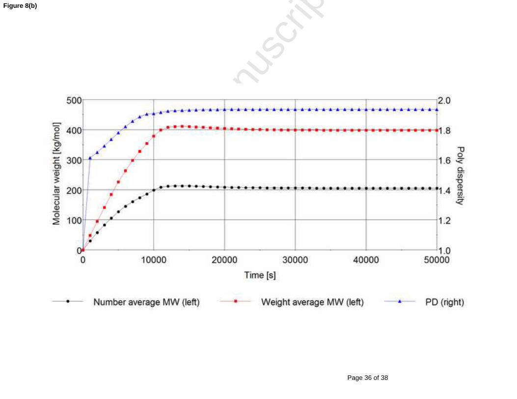
Mn, Mw and PD and PD of the growing polymer increased with time (Fig. 8). The polymer
produced in the pre-polymerization reactor possesses Mn and Mw of 27000 g mol-1 and 51000 g mol-1
respectively and a PD of 1.98, which lies between the PD of 1.5 and 2.5 of the polymer produced
from the existing plant. It is evident that an increase in polymer growth was achieved in the first loop
reactor from a quick comparison with the Mn of 205746 g mol-1 and Mw of 398085 g mol-1 of the
issuing pre-polymerization products, which resulted in a PD of 1.93 (Fig. 8 (b)). A plot of these values

Page 11 of 38
Accep
ted
Man
uscr
ipt
from the simulation of the Spheripol process is shown in Fig. 8 (c). Inferring from this graphical
representation indicate values of 215053 g mol-1 and 412558 g mol-1 for Mn and Mw respectively
with a PD of 1.92. The PD and MW in the second reactor remained almost constant. The second loop
reactor increased the yield of polymer as reflected in an increase in the polymer flow rate from
16860.42 kg hr-1 to 27181.42 kg hr-1 (Table 4) despite the constancy in PD and MW.
Fig. 8. Average molecular weight and polydispersity profile of produced polymer: (a) pre-
polymerization reactor, (b) 1st loop reactor, (c) 2nd loop reactor.
Validation of simulation
Simulation results shown in Table 4 predict conversions of 17.56%, 52.4%, and 54.91% in the pre-
polymerization, R1, and R2 respectively. Comparing these conversions with conversions achieved
from an existing plant under the same operating conditions in the bar chart of Fig. 9 below shows
absolute errors of 1.90 %, 1.69 %, and 3.02 % in the pre-polymerization, R1, and R2 respectively.
These are errors less than 10 % and considered acceptable for engineering applications.
Table 4. Material balance of simulation result
Fig. 9. Comparison and validation of polymer conversion rate for each reactor
Conclusion
A plethora of factors such as operating conditions, processing methods, catalysts, and the choice of
reactors influence the quality and efficiency of polymer processes. This difficulty has led to the
development of model based analysis of the Spheripol process for polyolefin production, particularly
in consideration of steady and dynamic state simulation. Deductions and conclusions from the work
carried out are as follows:
First, rigorous mathematical modeling of the reactors, namely the pre-polymerization reactor, first
loop reactor, and second loop reactor, was carried out to provide an accurate description of
physicochemical changes by way of conservation equations, polymerization reaction kinetics,
methods of moment, and population balance. Important process variables such as concentration,
density, temperature, and mass flow rate as well as MW and growth of the polymer chains were
considered in the formulation of the mathematical models.
Second, based on the developed mathematical model, a dynamic simulation was executed using
commercial operating and design data to identify the dynamic behavior of the process. The simulation

Page 12 of 38
Accep
ted
Man
uscr
ipt
results were compared with commercial data to verify the accuracy and effectiveness of this research.
The simulation predicted an overall conversion of 54.91 % with an associated error of 3.02 %. It is
concluded that this study can be extended for design and operational optimization of polyolefin
processes as well as other polymerization process without considerable modifications.
Acknowledgement
This research is funded by the LINC Program of Hanbat National University (2015) and the authors
would like to acknowledge for the assistance.

Page 13 of 38
Accep
ted
Man
uscr
ipt
REFERENCE
[1] B. A. Uvarov, V. I Tsevetkova, Polim. Protsessy Appar. Tecnol. Oformlenie Mat. Model
(1974), 165-168
[2] D. M. Lepski, A. M. Inkov, Sb. Tr. Vses. Ob’edin. Meftekim 13 (1977), 34-45
[3] M. A. Ferrero, M. G. Chiovetta, Polym.-Plast. Technol. Engng 29 (1990), 263-287
[4] J. R. Fried, Polymer Science and Technology, PrenticeHallPTR, (1996)
[5] N. G. McCrum, C. P. Buckley, C. B. Bucknall, second edition, Oxford, (1998)
[6] KOSHA, KOREA OCCUPATIONAL SAFETY & HEALTH AGENCY,
<www.kosha.or.kr/cms/board/Download.jsp?fileId=58539>
[7] A. G. Mattos Neto, J. C. Pinto, Chemical Engineering Science, 56 (2001), 4043-4057
[8] E. A. de Lucca, R. M. Filho, P. A. Melo, J. C. Pinto, Macromol. Symp. 271 (2008), 8-14
[9] J. J. Zacca, W. H. Ray, 48 (1993), 3743-3765
[10] T. J. Crowley, K. Y. Choi, Ind. Eng. Chem. Res., 36 (1997), 1419-1423
[11] D. W. Van Krevelen, Properties of Polymers, Elsevier, (2009)
[12] Z. H. Luo, Y. Zheng, Z. K. Cao, S. H. Wen, POLYMER ENGINEERING AND SCIENCE, (2007),
1643-1649
[13] Z. H. Luo, P. L. Su, W. Wu, Ind. Eng. Chem. Res., 49 (2010), 11232-11243
[14] Z. Liu, X. Zhang, H. Huang, J. Yi, W. Liu, W. Liu, H. Zhen, Q. Huang, K. Gao, M. Zhang, W.
Yang, Journal of Industrial and Engineering Chemistry, 18 (2012), 2217–2224
[15] J. Pinyocheep, S. K. Ayudhya, B. Jongsomjit, P. Praserthdam, Journal of Industrial and
Engineering Chemistry, 18 (2012), 1888–1892
[16] D. R. Burfield, I. D. Mckenzie, P. J. T. Tait, Polymer, 13 (1972), 303-326
[17] L. L. Bohm, Polymer, 19 (1978), 545-552
[18] J. Boor, Academic Press, New York
[19] H. M. Hutchinson, Ph.D. thesis, University of Wisconsin, Madison.
[20] PSE. <http://www.psenterprise.com>, (2015)

Page 14 of 38
Accep
ted
Man
uscr
ipt
List of Figures
Fig. 1. Block diagram of the loop reactor structure
Fig. 2. Schematic diagram of liquid polymerization reactors
Fig. 3. Monomer concentration profile with time and space: (a) pre-polymerization reactor, (b) 1st loop
reactor, (c) 2nd loop reactor.
Fig. 4. Polymer concentration profile of live polymer and dead polymer with time at reactor exit: (a)
pre-polymerization reactor, (b) 1st loop reactor, (c) 2nd loop reactor.
Fig. 5. Temperature profile with time at reactor exit: (a) pre-polymerization reactor, (b) 1st loop reactor,
(c) 2nd loop reactor.
Fig. 6. Controlled rate of inflow in cooling jacket: (a) 1st loop reactor, (b) 2nd loop reactor.
Fig. 7. Velocity profile with time and space: (a) pre-polymerization reactor, (b) 1st loop reactor, (c) 2nd
loop reactor.
Fig. 8. Average molecular weight and polydispersity profile of produced polymer: (a) pre-
polymerization reactor, (b) 1st loop reactor, (c) 2nd loop reactor.
Fig. 9. Comparison and validation of polymer conversion rate for each reactor

Page 15 of 38
Accep
ted
Man
uscr
ipt
List of Tables
Table 1. Design parameters of polymerization reactors
Table 2. Ziegler-Natta reaction mechanism for PP polymerization
Table 3. Ziegler-Natta reaction constant for PP polymerization
Table 4. Material balance of simulation result

Page 16 of 38
Accep
ted
Man
uscr
ipt
Table 1. Design parameters of polymerization reactor
Parameter Pre-polymerization reactor Polymerization loop reactor
Length of reactor 45 m 190 m
Diameter of tube 0.168 m 0.6 m
Diameter of jacket 0.273 m 0.8 m
Recycle ratio 75 153.3
Flowrate of cooling water
11.11 kg/s 222.22 kg/s
Table 2. Ziegler-Natta reaction mechanism for PP polymerization
Initiation
Propagation
Chain transfer to hydrogen
Chain transfer to monomer
Chain transfer to co-catalyst
Deactivation reactions
Spontaneous deactivation
Table 3. Ziegler-Natta reaction constant for PP polymerization
Reaction constant
kin : Initiation 4.97×10⁴ m3 mol-1 s-1 50000 J mol-1
kp : Propagation 4.97×10⁴ m3 mol-1 s-1 50000 J mol-1
ktr,H : Transfer to hydrogen 4.4×10³ m3 mol-1 s-1 50000 J mol-1
ktr,M : Transfer to monomer 6.16 m3 mol-1 s-1 50000 J mol-1
ktr,A : Transfer to co-catalyst 7.04×10⁻¹ m3 mol-1 s-1 50000 J mol-1
kd : Deactivation 7.92×10³ s-1 50000 J mol-1

Page 17 of 38
Accep
ted
Man
uscr
ipt
Table 4. Material balance of simulation result
Streamnumber
101 102 103 104 105 106 107 108 109
Description Catalysts Propylene R1outlet Propylene R2outlet Propylene R3outlet Top Bottom
Fraction kg h-1 kg h-1 kg h-1 kg h-1 kg h-1 kg h-1 kg h-1 kg h-1 kg h-1
Catalysts 12.35
Hydrogen 0.07 0.07 1.13 0.64
Propylene 1719.64 1396.02 27391.29 12240.54 15681.14 17586.29 15208.35 2377.94
Propane 180.29 180.49 2871.72 3075.53 1644.02 4734.58 4053.75 680.88
Polymer 335.77 16860.42 27181.42 27181.42
Total 12.35 1900 1912.35 30264.14 32176.49 17325.8 49502.29 19262.1 30240.19
T (℃) 10 10 20.3 45 70.1 45 70.2 70 70
P (bar) 40 35 35 35 35 35 35 18.4 2
ρ(kg m-3) 512 578 512 714 512 725

Page 18 of 38
Accep
ted
Man
uscr
ipt
*Graphical Abstract

Page 19 of 38
Accep
ted
Man
uscr
ipt
Figure 1

Page 20 of 38
Accep
ted
Man
uscr
ipt
Figure 2

Page 21 of 38
Accep
ted
Man
uscr
ipt
Figure 3(a)

Page 22 of 38
Accep
ted
Man
uscr
ipt
Figure 3(b)

Page 23 of 38
Accep
ted
Man
uscr
ipt
Figure 3(c)

Page 24 of 38
Accep
ted
Man
uscr
ipt
Figure 4(a)

Page 25 of 38
Accep
ted
Man
uscr
ipt
Figure 4(b)

Page 26 of 38
Accep
ted
Man
uscr
ipt
Figure 4(c)

Page 27 of 38
Accep
ted
Man
uscr
ipt
Figure 5(a)

Page 28 of 38
Accep
ted
Man
uscr
ipt
Figure 5(b)

Page 29 of 38
Accep
ted
Man
uscr
ipt
Figure 5(c)

Page 30 of 38
Accep
ted
Man
uscr
ipt
Figure 6(a)

Page 31 of 38
Accep
ted
Man
uscr
ipt
Figure 6(b)

Page 32 of 38
Accep
ted
Man
uscr
ipt
Figure 7(a)

Page 33 of 38
Accep
ted
Man
uscr
ipt
Figure 7(b)

Page 34 of 38
Accep
ted
Man
uscr
ipt
Figure 7(c)

Page 35 of 38
Accep
ted
Man
uscr
ipt
Figure 8(a)
Page 36 of 38
Accep
ted
Man
uscr
ipt
Figure 8(b)

Page 37 of 38
Accep
ted
Man
uscr
ipt
Figure 8(c)

Page 38 of 38
Accep
ted
Man
uscr
ipt
Figure 9