kill zone analysis for a bank-to-turn missile-target ... · pdf filekill zone analysis for a...
TRANSCRIPT

Kill Zone Analysis for a Bank-to-Turn
Missile-Target Engagement
by
Venkatraman Renganathan
A Thesis Presented in Partial Fulfillmentof the Requirements for the Degree
Master of Science
Approved July 2016 by theGraduate Supervisory Committee:
Armando A. Rodriguez, ChairPanagiotis ArtemiadisSpring Melody Berman
ARIZONA STATE UNIVERSITY
August 2016

ABSTRACT
With recent advances in missile and hypersonic vehicle technologies, the need for
being able to accurately simulate missile-target engagements has never been greater.
Within this research, we examine a fully integrated missile-target engagement envi-
ronment. A MATLAB based application is developed with 3D animation capabilities
to study missile-target engagement and visualize them. The high fidelity environment
is used to validate miss distance analysis with the results presented in relevant GNC
textbooks [51], [52] and to examine how the kill zone varies with critical engagement
parameters; e.g. initial engagement altitude, missile Mach, and missile maximum ac-
celeration. A ray-based binary search algorithm is used to estimate the kill zone
region; i.e. the set of initial target starting conditions such that it will be “killed”.
The results show what is expected. The kill zone increases with larger initial missile
Mach and maximum acceleration & decreases with higher engagement altitude and
higher target Mach. The environment is based on (1) a 6DOF bank-to-turn (BTT)
missile, (2) a full aerodynamic-stability derivative look up tables ranging over Mach
number, angle of attack and sideslip angle (3) a standard atmosphere model, (4) actu-
ator dynamics for each of the four cruciform fins, (5) seeker dynamics, (6) a nonlinear
autopilot, (7) a guidance system with three guidance algorithms (i.e. PNG, optimal,
differential game theory), (8) a 3DOF target model with three maneuverability mod-
els (i.e. constant speed, Shelton Turn & Climb, Riggs-Vergaz Turn & Dive). Each
of the subsystems are described within the research. The environment contains lin-
earization, model analysis and control design features. A gain scheduled nonlinear
BTT missile autopilot is presented here. Autopilot got sluggish as missile altitude
increased and got aggressive as missile mach increased. In short, the environment is
shown to be a very powerful tool for conducting missile-target engagement research -
a research that could address multiple missiles and advanced targets.
i

Dedicated to my parents and the loving memory of my brother Ravi
ii

ACKNOWLEDGMENTS
I want to thank the almighty for his blessings. First, I would like to express my
sincere gratitude to my MS thesis advisor Dr. Armando A. Rodriguez for showing
confidence in my work, his continuous motivation and support for my research, for
his patience, motivation, enthusiasm, and immense knowledge. His guidance helped
me throughout the course of the research and writing of this thesis. I could not have
imagined having a better advisor and mentor for my Masters studies. Besides my
thesis advisor, I would like to extend my gratitude to the rest of my thesis committee
Dr. Spring Berman and Dr. Panagiotis Artemiadis. I am grateful to all of the faculty
members who handled graduate courses for me at ASU.
I would also like to acknowledge the support of my fellow research mates Jesus
Aldaco Lopez(Thanks for those daily yoghurts & discussions), Zhichao Li, Xianglong
Lu, Nikhilesh Ravishankar, Kamalakannan Thammireddi Vajram, Dibyadeep Bose &
Michael Thompson for standing through as my pillars of strength during all times.
Thanks to David Phelps for sharing my burden. I take this opportunity to thank my
friends Karan Puttannaiah, Kaustav Mondal, Ashfaque Bin Shafique, Rakesh Joshi,
Parag Mitra, Sai Akshit Kumar Gampa, Madhurima Poore & Vignesh Narayanan
for their tremendous support and stimulating discussions about my research which
kept me motivated to complete my Masters thesis. Immense thanks to Shruti Anand
for introducing me to LATEX. Special thanks to Justin Echols for letting me use his
printer as much as I wanted. I wish all of them great and exciting careers for their
future. An heartfelt thanks to my past roommates Sudarsan, Narasimhan & Hari and
my present roommates Pranav & Shishir for being there for me anytime I wanted.
Finally, I would like to dedicate this work to my lovely parents Mr. V. Renganathan
& Mrs. Brinda Renganathan for their love, encouragement, support and attention.
Wherever you are my dear Ravi, this achievement is because of you.
iii
TABLE OF CONTENTS
Page
LIST OF TABLES . . . . . . . . . . . . . . . . . . . . . . . . . . . . . . . . . . . . . . . . . . . . . . . . . . . . . . . . . ix
LIST OF FIGURES . . . . . . . . . . . . . . . . . . . . . . . . . . . . . . . . . . . . . . . . . . . . . . . . . . . . . . . . xi
LIST OF SYMBOLS . . . . . . . . . . . . . . . . . . . . . . . . . . . . . . . . . . . . . . . . . . . . . . . . . . . . . . . xx
CHAPTER
1 INTRODUCTION & OVERVIEW OF WORK . . . . . . . . . . . . . . . . . . . . . . . . 1
1.1 Introduction and Motivation . . . . . . . . . . . . . . . . . . . . . . . . . . . . . . . . . . . . . 1
1.2 Literature Survey: Missile Guidance System - State of the Field . . . . 2
1.3 Goals and Contributions . . . . . . . . . . . . . . . . . . . . . . . . . . . . . . . . . . . . . . . . 7
1.4 Contributions of Work: Questions to be Addressed . . . . . . . . . . . . . . . . 8
1.5 Overview of Thesis . . . . . . . . . . . . . . . . . . . . . . . . . . . . . . . . . . . . . . . . . . . . . . 10
1.6 Organization of Thesis . . . . . . . . . . . . . . . . . . . . . . . . . . . . . . . . . . . . . . . . . . 13
1.7 Summary and Conclusions . . . . . . . . . . . . . . . . . . . . . . . . . . . . . . . . . . . . . . 15
2 MISSILE & ACTUATOR DYNAMICS . . . . . . . . . . . . . . . . . . . . . . . . . . . . . . . . 16
2.1 Introduction and Overview . . . . . . . . . . . . . . . . . . . . . . . . . . . . . . . . . . . . . . 16
2.2 Inertial, Vehicle and Body Frames . . . . . . . . . . . . . . . . . . . . . . . . . . . . . . . 16
2.2.1 Inertial Frame . . . . . . . . . . . . . . . . . . . . . . . . . . . . . . . . . . . . . . . . . . . 17
2.2.2 Vehicle Frame . . . . . . . . . . . . . . . . . . . . . . . . . . . . . . . . . . . . . . . . . . . 18
2.2.3 Body Frame . . . . . . . . . . . . . . . . . . . . . . . . . . . . . . . . . . . . . . . . . . . . . 19
2.3 Thrust Profile and Variable-Mass Dynamics . . . . . . . . . . . . . . . . . . . . . . 26
2.4 Missile Aerodynamics . . . . . . . . . . . . . . . . . . . . . . . . . . . . . . . . . . . . . . . . . . . 33
2.4.1 Stability and Control Derivatives . . . . . . . . . . . . . . . . . . . . . . . . . . 34
2.4.2 Aerodynamic (Wind) Frame . . . . . . . . . . . . . . . . . . . . . . . . . . . . . . 44
2.4.3 Force and Moment Coefficients . . . . . . . . . . . . . . . . . . . . . . . . . . . . 46
2.4.4 Aerodynamic Forces (Fx, Fy, Fz) and Moments (L, M, N) . . . 49
iv
CHAPTER Page
2.4.5 Gravitational Forces and Moments . . . . . . . . . . . . . . . . . . . . . . . . 49
2.5 Equations of Motion for the Missile . . . . . . . . . . . . . . . . . . . . . . . . . . . . . . 51
2.6 Actuator Dynamics . . . . . . . . . . . . . . . . . . . . . . . . . . . . . . . . . . . . . . . . . . . . . 53
2.7 Summary and Conclusions . . . . . . . . . . . . . . . . . . . . . . . . . . . . . . . . . . . . . . 54
3 LINEARIZED MISSILE MODEL ANALYSIS . . . . . . . . . . . . . . . . . . . . . . . . . 55
3.1 Introduction and Overview . . . . . . . . . . . . . . . . . . . . . . . . . . . . . . . . . . . . . . 55
3.2 Linear Equations of Motion . . . . . . . . . . . . . . . . . . . . . . . . . . . . . . . . . . . . . 56
3.3 Calculation of Equilibrium Points . . . . . . . . . . . . . . . . . . . . . . . . . . . . . . . . 69
3.4 Scaled Linear BTT Missile State-Space System . . . . . . . . . . . . . . . . . . . 72
3.5 Discussion of BTT Missile Natural Modes (Eigenvalues) . . . . . . . . . . . 92
3.5.1 Longitudinal Dynamics . . . . . . . . . . . . . . . . . . . . . . . . . . . . . . . . . . . 93
3.5.2 Lateral Dynamics . . . . . . . . . . . . . . . . . . . . . . . . . . . . . . . . . . . . . . . . 100
3.6 Missile Static Analysis - Elevator & Throttle Trim . . . . . . . . . . . . . . . . 108
3.7 Summary and Conclusions . . . . . . . . . . . . . . . . . . . . . . . . . . . . . . . . . . . . . . 113
4 MISSILE SEEKER / NAVIGATION & GUIDANCE . . . . . . . . . . . . . . . . . . . 114
4.1 Introduction and Overview . . . . . . . . . . . . . . . . . . . . . . . . . . . . . . . . . . . . . . 114
4.2 Seeker Frame . . . . . . . . . . . . . . . . . . . . . . . . . . . . . . . . . . . . . . . . . . . . . . . . . . . 115
4.3 Seeker Dynamics. . . . . . . . . . . . . . . . . . . . . . . . . . . . . . . . . . . . . . . . . . . . . . . . 118
4.3.1 Seeker Model Software Algorithm . . . . . . . . . . . . . . . . . . . . . . . . . 118
4.3.2 Seeker Dynamics Block Diagram . . . . . . . . . . . . . . . . . . . . . . . . . . 123
4.4 Guidance Algorithms . . . . . . . . . . . . . . . . . . . . . . . . . . . . . . . . . . . . . . . . . . . 124
4.4.1 Proportional Navigation Guidance . . . . . . . . . . . . . . . . . . . . . . . . 124
4.4.2 Optimal Control Theory Guidance . . . . . . . . . . . . . . . . . . . . . . . . 125
4.4.3 Differential Game Theory Guidance . . . . . . . . . . . . . . . . . . . . . . . 127
v

CHAPTER Page
4.5 Summary and Conclusions . . . . . . . . . . . . . . . . . . . . . . . . . . . . . . . . . . . . . . 128
5 TARGET MODELING . . . . . . . . . . . . . . . . . . . . . . . . . . . . . . . . . . . . . . . . . . . . . . 129
5.1 Introduction and Overview . . . . . . . . . . . . . . . . . . . . . . . . . . . . . . . . . . . . . . 129
5.2 3DOF Target Dynamics . . . . . . . . . . . . . . . . . . . . . . . . . . . . . . . . . . . . . . . . . 129
5.3 Straight Flight with No Maneuver. . . . . . . . . . . . . . . . . . . . . . . . . . . . . . . . 130
5.4 Sheldon Turn & Climb Maneuver . . . . . . . . . . . . . . . . . . . . . . . . . . . . . . . . 130
5.5 Riggs Vergaz Turn & Dive Maneuver . . . . . . . . . . . . . . . . . . . . . . . . . . . . . 132
5.6 Summary and Conclusions . . . . . . . . . . . . . . . . . . . . . . . . . . . . . . . . . . . . . . 134
6 BTT MISSILE AUTOPILOT . . . . . . . . . . . . . . . . . . . . . . . . . . . . . . . . . . . . . . . . 135
6.1 Introduction and Overview . . . . . . . . . . . . . . . . . . . . . . . . . . . . . . . . . . . . . . 135
6.2 Control Law Formulation . . . . . . . . . . . . . . . . . . . . . . . . . . . . . . . . . . . . . . . . 140
6.2.1 Gain Scheduling of Linear Parameter Varying System . . . . . . 144
6.3 BTT Logic . . . . . . . . . . . . . . . . . . . . . . . . . . . . . . . . . . . . . . . . . . . . . . . . . . . . . 145
6.4 Angular Rate Command Generator . . . . . . . . . . . . . . . . . . . . . . . . . . . . . . 146
6.5 Mixed Fin Command Generator: p-q-r-thrust/drag . . . . . . . . . . . . . . . . 147
6.6 ILAAT De-Mixer: Four Fin Force Commands to Actuators . . . . . . . . 148
6.7 ILAAT Mixer: 3 Effective Aileron, Flapperon, Rudder Controls . . . . 148
6.8 Nonlinear Autopilot Simulation Results . . . . . . . . . . . . . . . . . . . . . . . . . . 149
6.9 Autopilot Linearization . . . . . . . . . . . . . . . . . . . . . . . . . . . . . . . . . . . . . . . . . 162
6.9.1 Assumptions about Steady Flight Conditions . . . . . . . . . . . . . . 162
6.9.2 Innermost Loop . . . . . . . . . . . . . . . . . . . . . . . . . . . . . . . . . . . . . . . . . . 162
6.9.3 Intermediate Loop . . . . . . . . . . . . . . . . . . . . . . . . . . . . . . . . . . . . . . . 167
6.10 Summary and Conclusions . . . . . . . . . . . . . . . . . . . . . . . . . . . . . . . . . . . . . . 183
7 NUMERICAL INTEGRATION. . . . . . . . . . . . . . . . . . . . . . . . . . . . . . . . . . . . . . . 184
vi

CHAPTER Page
7.1 Introduction and Overview . . . . . . . . . . . . . . . . . . . . . . . . . . . . . . . . . . . . . . 184
7.2 Runge-Kutta(RK) Integration Methods . . . . . . . . . . . . . . . . . . . . . . . . . . 185
7.2.1 Runge-Kutta 1st Method . . . . . . . . . . . . . . . . . . . . . . . . . . . . . . . . . 186
7.2.2 Runge-Kutta 2nd Method . . . . . . . . . . . . . . . . . . . . . . . . . . . . . . . . . 186
7.2.3 Runge-Kutta 4th Method . . . . . . . . . . . . . . . . . . . . . . . . . . . . . . . . . 187
7.2.4 Adaptive Step Size - Runge-Kutta-Fehlberg Method . . . . . . . . 188
7.3 Nominal Step Size Selection using Engagement Geometry Analysis . 189
7.4 Summary and Conclusions . . . . . . . . . . . . . . . . . . . . . . . . . . . . . . . . . . . . . . 195
8 MISS DISTANCE ANALYSIS . . . . . . . . . . . . . . . . . . . . . . . . . . . . . . . . . . . . . . . . 196
8.1 Introduction and Overview . . . . . . . . . . . . . . . . . . . . . . . . . . . . . . . . . . . . . . 196
8.2 Miss Distance Dependence on Proportional Gain . . . . . . . . . . . . . . . . . . 197
8.3 Miss Distance Dependence on Initial Engagement Altitude . . . . . . . . . 199
8.4 Miss Distance Dependence on Missile Maximum Acceleration . . . . . . 202
8.5 Miss Distance Dependence on Initial Missile Mach . . . . . . . . . . . . . . . . 207
8.6 Miss Distance Dependence on Target Maneuver . . . . . . . . . . . . . . . . . . . 209
8.7 Miss Distance Dependence on Target Aspect . . . . . . . . . . . . . . . . . . . . . . 212
8.8 Miss Distance Dependence on Initial Target Range . . . . . . . . . . . . . . . . 215
8.9 Summary and Conclusions . . . . . . . . . . . . . . . . . . . . . . . . . . . . . . . . . . . . . . 218
9 KILL ZONE COMPUTATION & ANALYSIS . . . . . . . . . . . . . . . . . . . . . . . . . 219
9.1 Introduction and Overview . . . . . . . . . . . . . . . . . . . . . . . . . . . . . . . . . . . . . . 219
9.2 Binary Search Algorithm . . . . . . . . . . . . . . . . . . . . . . . . . . . . . . . . . . . . . . . . 220
9.3 Kill Zone Dependence on Initial Engagement Altitude Variation . . . . 222
9.4 Kill Zone Dependence on Missile Maximum Acceleration Variation . 224
9.5 Kill Zone Dependence on Initial Missile Mach Variation . . . . . . . . . . . 225
vii

CHAPTER Page
9.6 Kill Zone Dependence on Initial Target Mach Variation . . . . . . . . . . . . 226
9.7 Kill Zone Dependence on Initial Aspect Variation . . . . . . . . . . . . . . . . . 228
9.8 Kill Zone Dependence on Proportional Gain Variation . . . . . . . . . . . . . 232
9.9 Summary and Conclusions . . . . . . . . . . . . . . . . . . . . . . . . . . . . . . . . . . . . . . 234
10 MISSILE-TARGET 3D ANIMATION USING MATLAB . . . . . . . . . . . . . . . 235
10.1 Introduction and Overview . . . . . . . . . . . . . . . . . . . . . . . . . . . . . . . . . . . . . . 235
10.2 Interactive GUI Developement . . . . . . . . . . . . . . . . . . . . . . . . . . . . . . . . . . . 236
10.3 3D Animation using MATLAB VRML Toolbox . . . . . . . . . . . . . . . . . . . 237
10.4 Simulation Results & Analysis . . . . . . . . . . . . . . . . . . . . . . . . . . . . . . . . . . . 240
10.5 Summary and Conclusions . . . . . . . . . . . . . . . . . . . . . . . . . . . . . . . . . . . . . . 247
11 SUMMARY & DIRECTIONS FOR FUTURE RESEARCH. . . . . . . . . . . . . 248
11.1 Summary of Work . . . . . . . . . . . . . . . . . . . . . . . . . . . . . . . . . . . . . . . . . . . . . . 248
11.2 Directions for Future Research . . . . . . . . . . . . . . . . . . . . . . . . . . . . . . . . . . . 249
REFERENCES . . . . . . . . . . . . . . . . . . . . . . . . . . . . . . . . . . . . . . . . . . . . . . . . . . . . . . . . . . . . 251
APPENDIX
A C CODE - BINARY SEARCH ALGORITHM . . . . . . . . . . . . . . . . . . . . . . . . . 258
B MATLAB CODE - MISSILE PLANT & AUTOPILOT ANALYSIS . . . . . 264
viii

LIST OF TABLES
Table Page
2.1 Thrust Profile Equations . . . . . . . . . . . . . . . . . . . . . . . . . . . . . . . . . . . . . . . . . . . 29
2.2 Missile’s Time-Zero Mass and Moment of Inertia . . . . . . . . . . . . . . . . . . . . . 31
2.3 Stability Derivatives and Parameter Dependence . . . . . . . . . . . . . . . . . . . . . 35
2.4 Control Derivatives and Parameter Dependence . . . . . . . . . . . . . . . . . . . . . . 35
2.5 Body Frame Force and Moment Notation . . . . . . . . . . . . . . . . . . . . . . . . . . . . 47
3.1 Time-Zero Mass Properties for Altitude = 10 kft . . . . . . . . . . . . . . . . . . . . . 104
3.2 Fuel Spent Mass Properties for Altitude = 10 kft . . . . . . . . . . . . . . . . . . . . . 104
3.3 Time-Zero Mass Properties for Altitude = 40 kft . . . . . . . . . . . . . . . . . . . . . 105
3.4 Fuel Spent Mass Properties for Altitude = 40 kft . . . . . . . . . . . . . . . . . . . . . 105
3.5 α Variation for Alt. = 40 kft, Mach = 2.0 . . . . . . . . . . . . . . . . . . . . . . . . . . . 106
3.6 Mach Variation for Alt. = 40 kft, α = 15 deg . . . . . . . . . . . . . . . . . . . . . . . . 106
4.1 Proportional Guidance Gains . . . . . . . . . . . . . . . . . . . . . . . . . . . . . . . . . . . . . . . 125
6.1 Autopilot Gains . . . . . . . . . . . . . . . . . . . . . . . . . . . . . . . . . . . . . . . . . . . . . . . . . . . 147
6.2 Flight Conditions for Nonlinear Autopilot Simulations . . . . . . . . . . . . . . . . 149
7.1 Comparison of Runge-Kutta Integration Methods . . . . . . . . . . . . . . . . . . . . 189
7.2 Flight Conditions for Miss Distance vs Integration Step Size . . . . . . . . . . 190
8.1 Flight Conditions for Miss Distance vs Proportional Gain . . . . . . . . . . . . . 197
8.2 Flight Conditions for Miss Distance vs Engagement Altitude . . . . . . . . . . 200
8.3 Flight Conditions for Miss Distance vs Missile Maximum Acceleration . 203
8.4 Flight Conditions for Miss Distance vs Missile Mach . . . . . . . . . . . . . . . . . . 208
8.5 Flight Conditions for Miss Distance vs Target Maneuver . . . . . . . . . . . . . . 210
8.6 Flight Conditions for Miss Distance vs Target Aspect . . . . . . . . . . . . . . . . . 212
8.7 Flight Conditions for Miss Distance vs Target Range . . . . . . . . . . . . . . . . . 216
9.1 Flight Conditions for Kill Zone vs Engagement Altitude . . . . . . . . . . . . . . 222
ix
Table Page
9.2 Flight Conditions for Kill Zone vs Missile Maximum Acceleration. . . . . . 224
9.3 Flight Conditions for Kill Zone vs Missile Mach . . . . . . . . . . . . . . . . . . . . . . 225
9.4 Flight Conditions for Kill Zone vs Target Mach . . . . . . . . . . . . . . . . . . . . . . 227
9.5 Flight Conditions for Kill Zone vs Target Aspect . . . . . . . . . . . . . . . . . . . . . 228
9.6 Flight Conditions for Kill Zone vs Proportional Gain . . . . . . . . . . . . . . . . . 233
10.1 GUI Flight Conditions Selection for Missile-Target Engagement . . . . . . . 237
10.2 Flight Conditions for MATLAB & C Simulations . . . . . . . . . . . . . . . . . . . . . 241
x

LIST OF FIGURES
Figure Page
1.1 Information Flow for Missile-Target Engagement. . . . . . . . . . . . . . . . . . . . . 11
1.2 Organization of MATLAB Program: 3 Modules. . . . . . . . . . . . . . . . . . . . . . 12
2.1 Local Inertial Frame with missile and target flight paths . . . . . . . . . . . . . . 17
2.2 Visualization of Inertial and Vehicle Frames . . . . . . . . . . . . . . . . . . . . . . . . . . 18
2.3 Visualization of Body Axes and Velocities . . . . . . . . . . . . . . . . . . . . . . . . . . . 19
2.4 Visualization of Euler Angles . . . . . . . . . . . . . . . . . . . . . . . . . . . . . . . . . . . . . . . 20
2.5 Visualization of N2 and N3 in Y bZb plane. . . . . . . . . . . . . . . . . . . . . . . . . . . . 24
2.6 Visualization of N1 and N3 in Xb x Zv plane. . . . . . . . . . . . . . . . . . . . . . . . . 25
2.7 Relationship between Euler Angles and Body Rates. . . . . . . . . . . . . . . . . . . 25
2.8 Missile Two-Stage Thrust Profile . . . . . . . . . . . . . . . . . . . . . . . . . . . . . . . . . . . . 27
2.9 Visualization of CG0 and Vb . . . . . . . . . . . . . . . . . . . . . . . . . . . . . . . . . . . . . . . . 31
2.10 CD - Drag from Pitch Fin Deflection - depends on δq, Mach-1, α-1 . . . . . 36
2.11 CDT - Base Drag due to Mach-2 . . . . . . . . . . . . . . . . . . . . . . . . . . . . . . . . . . . . 36
2.12 CLβ - Roll Moment from Sideslip - depends on Mach-1, α-1 . . . . . . . . . . . 37
2.13 CLδp - Roll Moment from Roll Fin Deflection - depends on Mach-1, α-1 37
2.14 CLP - Roll Damping Moment - Pitch rate - depends on Mach-1, α-3 . . . 38
2.15 CMα - Pitch Moment from Angle of Attack - depends on Mach-1, α-4 . . 38
2.16 CMδq- Pitch Moment from Pitch Fin Deflection - depends on Mach-1,
α-2 . . . . . . . . . . . . . . . . . . . . . . . . . . . . . . . . . . . . . . . . . . . . . . . . . . . . . . . . . . . . . . . 39
2.17 CMq - Pitch Moment from Pitch Fin Deflection - depends on Mach-2,
α-3 . . . . . . . . . . . . . . . . . . . . . . . . . . . . . . . . . . . . . . . . . . . . . . . . . . . . . . . . . . . . . . . 39
2.18 CNα - Lift due to Mach-1 . . . . . . . . . . . . . . . . . . . . . . . . . . . . . . . . . . . . . . . . . . . 40
2.19 CNβ - Yaw Moment from Sideslip - depends on Mach-1, α-1 . . . . . . . . . . . 40
2.20 CNδq - Lift from Pitch Fin Deflection - depends on Mach-1, α-2 . . . . . . . . 41
xi

Figure Page
2.21 CNδr - Yaw Moment from Yaw Fin Deflection - depends on Mach-1, β-1 41
2.22 CNR - Yaw Damping Moment - Yaw Rate - depends on Mach-2, β-2 . . . 42
2.23 CYβ - Side Force from Sideslip - depends on Mach-1, α-1 . . . . . . . . . . . . . . 42
2.24 CYδr - Side Force from Yaw Fin Deflection - depends on Mach-1, β-1 . . . 43
2.25 Scheduled Gain . . . . . . . . . . . . . . . . . . . . . . . . . . . . . . . . . . . . . . . . . . . . . . . . . . . . 43
2.26 Aerodynamic Force, Body Velocity and Aerodynamic Angles . . . . . . . . . . 44
2.27 Visualization of Sideslip Angle, β . . . . . . . . . . . . . . . . . . . . . . . . . . . . . . . . . . . 45
2.28 Visualization of Angle of Attack, α . . . . . . . . . . . . . . . . . . . . . . . . . . . . . . . . . . 45
2.29 Body Frame Axis System and Notation . . . . . . . . . . . . . . . . . . . . . . . . . . . . . . 47
2.30 Model for Nonlinear Fin Actuators / Servomechanisms . . . . . . . . . . . . . . . 53
3.1 Frequency Response - Ay vs Aileron - Altitude Varying . . . . . . . . . . . . . . . 77
3.2 Frequency Response - Ay vs Rudder - Altitude Varying . . . . . . . . . . . . . . . 78
3.3 Frequency Response - Az vs Elevator - Altitude Varying . . . . . . . . . . . . . . 78
3.4 Frequency Response - φ vs Aileron - Altitude Varying . . . . . . . . . . . . . . . . 79
3.5 Frequency Response - φ vs Rudder - Altitude Varying . . . . . . . . . . . . . . . . 79
3.6 Frequency Response - θ vs Elevator - Altitude Varying. . . . . . . . . . . . . . . . 80
3.7 Frequency Response - β vs Aileron - Altitude Varying . . . . . . . . . . . . . . . . 80
3.8 Frequency Response - β vs Rudder - Altitude Varying . . . . . . . . . . . . . . . . 81
3.9 Frequency Response - α vs Elevator - Altitude Varying . . . . . . . . . . . . . . . 81
3.10 Frequency Response - γ vs Elevator - Altitude Varying . . . . . . . . . . . . . . . 82
3.11 Frequency Response - P vs Aileron - Altitude Varying . . . . . . . . . . . . . . . . 82
3.12 Frequency Response - P vs Rudder - Altitude Varying . . . . . . . . . . . . . . . . 83
3.13 Frequency Response - Q vs Elevator - Altitude Varying . . . . . . . . . . . . . . . 83
3.14 Frequency Response - R vs Aileron - Altitude Varying . . . . . . . . . . . . . . . . 84
xii

Figure Page
3.15 Frequency Response - R vs Rudder - Altitude Varying . . . . . . . . . . . . . . . . 84
3.16 Frequency Response - Ay vs Aileron - Mach Varying . . . . . . . . . . . . . . . . . . 85
3.17 Frequency Response - Ay vs Rudder - Mach Varying . . . . . . . . . . . . . . . . . . 85
3.18 Frequency Response - Az vs Elevator - Mach Varying . . . . . . . . . . . . . . . . . 86
3.19 Frequency Response - φ vs Aileron - Mach Varying . . . . . . . . . . . . . . . . . . . 86
3.20 Frequency Response - φ vs Rudder - Mach Varying . . . . . . . . . . . . . . . . . . . 87
3.21 Frequency Response - θ vs Elevator - Mach Varying . . . . . . . . . . . . . . . . . . 87
3.22 Frequency Response - β vs Aileron - Mach Varying . . . . . . . . . . . . . . . . . . . 88
3.23 Frequency Response - β vs Rudder - Mach Varying . . . . . . . . . . . . . . . . . . . 88
3.24 Frequency Response - α vs Elevator - Mach Varying . . . . . . . . . . . . . . . . . . 89
3.25 Frequency Response - γ vs Elevator - Mach Varying . . . . . . . . . . . . . . . . . . 89
3.26 Frequency Response - P vs Aileron - Mach Varying . . . . . . . . . . . . . . . . . . . 90
3.27 Frequency Response - P vs Rudder - Mach Varying . . . . . . . . . . . . . . . . . . . 90
3.28 Frequency Response - Q vs Elevator - Mach Varying . . . . . . . . . . . . . . . . . . 91
3.29 Frequency Response - R vs Aileron - Mach Varying . . . . . . . . . . . . . . . . . . . 91
3.30 Frequency Response - R vs Rudder - Mach Varying. . . . . . . . . . . . . . . . . . . 92
3.31 Longitunal Plant RHP Zero Dynamics - Altitude Varying . . . . . . . . . . . . . 96
3.32 Longitunal Plant RHP Zero Dynamics - Altitude Varying With Mach. . 97
3.33 Longitunal Plant RHP Zero Dynamics - α Varying . . . . . . . . . . . . . . . . . . . 97
3.34 Longitunal Plant RHP Zero Dynamics - Mach Varying . . . . . . . . . . . . . . . 98
3.35 Longitunal Plant RHP Pole Dynamics - Altitude Varying . . . . . . . . . . . . . 98
3.36 Longitunal Plant RHP Pole Dynamics - Altitude Varying With Mach . . 99
3.37 Longitunal Plant RHP Pole Dynamics - α Varying . . . . . . . . . . . . . . . . . . . 99
3.38 Longitunal Plant RHP Pole Dynamics - Mach Varying . . . . . . . . . . . . . . . . 100
xiii

Figure Page
3.39 Lateral Plant RHP Pole Dynamics - Altitude Varying . . . . . . . . . . . . . . . . 101
3.40 Lateral Plant RHP Pole Dynamics - α Varying . . . . . . . . . . . . . . . . . . . . . . . 101
3.41 Lateral Plant Pole-Zero Map - α Varying . . . . . . . . . . . . . . . . . . . . . . . . . . . . 102
3.42 Lateral Plant Pole-Zero Map - Altitude Varying . . . . . . . . . . . . . . . . . . . . . . 102
3.43 Level Flight - Elevator Trim for Altitude . . . . . . . . . . . . . . . . . . . . . . . . . . . . 109
3.44 Level Flight - Elevator Trim for α . . . . . . . . . . . . . . . . . . . . . . . . . . . . . . . . . . . 109
3.45 Level Flight - Throttle Trim . . . . . . . . . . . . . . . . . . . . . . . . . . . . . . . . . . . . . . . . 110
3.46 Level Flight - Throttle Trim for Mach . . . . . . . . . . . . . . . . . . . . . . . . . . . . . . . 110
3.47 Level Flight - Mach Varying with Altitude . . . . . . . . . . . . . . . . . . . . . . . . . . . 111
3.48 Level Flight - Mach Varying with α . . . . . . . . . . . . . . . . . . . . . . . . . . . . . . . . . 111
3.49 Level Flight - α Varying with Altitude . . . . . . . . . . . . . . . . . . . . . . . . . . . . . . . 112
4.1 Block Diagram of Seeker/Navigation Model Algorithm . . . . . . . . . . . . . . . . 115
4.2 Seeker Frame orientation with respect to Seeker Gimbal Angles . . . . . . . 116
4.3 Seeker Frame Line-of-Sight Angles (σy, σp) and Range . . . . . . . . . . . . . . . . 117
4.4 Visualization of Vehicle Relative Separation . . . . . . . . . . . . . . . . . . . . . . . . . . 120
4.5 Commanded Gimbal Rate Generator . . . . . . . . . . . . . . . . . . . . . . . . . . . . . . . . 121
4.6 Block Diagram of Seeker Dynamics . . . . . . . . . . . . . . . . . . . . . . . . . . . . . . . . . . 123
4.7 Proportional Navigation Guidance . . . . . . . . . . . . . . . . . . . . . . . . . . . . . . . . . . 124
4.8 Optimal Control Theory Guidance . . . . . . . . . . . . . . . . . . . . . . . . . . . . . . . . . . 125
5.1 Sheldon Evasive Maneuver, Viewed from target-to-missile. . . . . . . . . . . . . 131
5.2 Riggs Vergaz Evasive Maneuver, Viewed from target-to-missile. . . . . . . . 133
6.1 An Asymmetrical EMRAAT Missile . . . . . . . . . . . . . . . . . . . . . . . . . . . . . . . . . 136
6.2 An Asymmetrical EMRAAT Missile Dimesions . . . . . . . . . . . . . . . . . . . . . . . 137
6.3 Block diagram of BTT Missile Autopilot . . . . . . . . . . . . . . . . . . . . . . . . . . . . . 139
xiv
Figure Page
6.4 Determination of Commanded Roll Angle from Ayc & Azc . . . . . . . . . . . . . 139
6.5 Post Flight Analysis - Missile Target Engagement . . . . . . . . . . . . . . . . . . . . 150
6.6 Post Flight Analysis - α Profile . . . . . . . . . . . . . . . . . . . . . . . . . . . . . . . . . . . . . 150
6.7 Post Flight Analysis - β Profile . . . . . . . . . . . . . . . . . . . . . . . . . . . . . . . . . . . . . 151
6.8 Post Flight Analysis - Range Profile . . . . . . . . . . . . . . . . . . . . . . . . . . . . . . . . . 151
6.9 Post Flight Analysis - Mach Profile . . . . . . . . . . . . . . . . . . . . . . . . . . . . . . . . . . 152
6.10 Post Flight Analysis - Fin 1 Deflection Profile . . . . . . . . . . . . . . . . . . . . . . . . 152
6.11 Post Flight Analysis - Fin 2 Deflection Profile . . . . . . . . . . . . . . . . . . . . . . . . 153
6.12 Post Flight Analysis - Fin 3 Deflection Profile . . . . . . . . . . . . . . . . . . . . . . . . 153
6.13 Post Flight Analysis - Fin 4 Deflection Profile . . . . . . . . . . . . . . . . . . . . . . . . 154
6.14 Post Flight Analysis - Fin 1 Rate Profile . . . . . . . . . . . . . . . . . . . . . . . . . . . . . 154
6.15 Post Flight Analysis - Fin 2 Rate Profile . . . . . . . . . . . . . . . . . . . . . . . . . . . . . 155
6.16 Post Flight Analysis - Fin 3 Rate Profile . . . . . . . . . . . . . . . . . . . . . . . . . . . . . 155
6.17 Post Flight Analysis - Fin 4 Rate Profile . . . . . . . . . . . . . . . . . . . . . . . . . . . . . 156
6.18 Post Flight Analysis - Air Density Profile . . . . . . . . . . . . . . . . . . . . . . . . . . . . 156
6.19 Post Flight Analysis - SOS Profile . . . . . . . . . . . . . . . . . . . . . . . . . . . . . . . . . . . 157
6.20 Post Flight Analysis - Dynamic Viscosity Profile . . . . . . . . . . . . . . . . . . . . . 157
6.21 Post Flight Analysis - Kinematic Viscosity Profile . . . . . . . . . . . . . . . . . . . . 158
6.22 Post Flight Analysis - Acceleration in Y Direction Profile . . . . . . . . . . . . . 158
6.23 Post Flight Analysis - Acceleration in Z Direction Profile . . . . . . . . . . . . . 159
6.24 Post Flight Analysis - Aileron Profile . . . . . . . . . . . . . . . . . . . . . . . . . . . . . . . . 159
6.25 Post Flight Analysis - Elevator Profile . . . . . . . . . . . . . . . . . . . . . . . . . . . . . . . 160
6.26 Post Flight Analysis - Rudder Profile . . . . . . . . . . . . . . . . . . . . . . . . . . . . . . . . 160
6.27 Post Flight Analysis - Roll Angle Profile . . . . . . . . . . . . . . . . . . . . . . . . . . . . . 161
xv
Figure Page
6.28 Post Flight Analysis - Role Rate Profile . . . . . . . . . . . . . . . . . . . . . . . . . . . . . 161
6.29 Block Diagram of Autopilot Innermost Loop . . . . . . . . . . . . . . . . . . . . . . . . . 162
6.30 Block Diagram of Autopilot Intermediate Loop. . . . . . . . . . . . . . . . . . . . . . . 167
6.31 Ki − 1st Channel Frequency Response - Altitude Varying . . . . . . . . . . . . . 169
6.32 Ki − 2nd Channel Frequency Response - Altitude Varying . . . . . . . . . . . . . 169
6.33 Ki − 3rd Channel Frequency Response - Altitude Varying . . . . . . . . . . . . . 170
6.34 Open Loop Channel 1 Frequency Response - Altitude Varying . . . . . . . . . 170
6.35 Open Loop Channel 2 Frequency Response - Altitude Varying . . . . . . . . . 171
6.36 Open Loop Channel 3 Frequency Response - Altitude Varying . . . . . . . . . 171
6.37 Inner Loop Complementary Sensitivity Pc vs P - Altitude Varying . . . . . 172
6.38 Inner Loop Complementary Sensitivity Qc vs Q - Altitude Varying . . . . 172
6.39 Inner Loop Complementary Sensitivity Rc vs R - Altitude Varying . . . . 173
6.40 Intermediate Loop φ Channel Sensitivities - Altitude Varying . . . . . . . . . 173
6.41 Intermediate Loop α Channel Sensitivities - Altitude Varying . . . . . . . . . 174
6.42 Intermediate Loop β Channel Sensitivities - Altitude Varying . . . . . . . . . 174
6.43 Ki − 1st Channel Frequency Response - Mach Varying . . . . . . . . . . . . . . . . 176
6.44 Ki − 2nd Channel Frequency Response - Mach Varying . . . . . . . . . . . . . . . 177
6.45 Ki − 3rd Channel Frequency Response - Mach Varying . . . . . . . . . . . . . . . . 177
6.46 Open Loop Channel 1 Frequency Response - Mach Varying . . . . . . . . . . . 178
6.47 Open Loop Channel 2 Frequency Response - Mach Varying . . . . . . . . . . . 178
6.48 Open Loop Channel 3 Frequency Response - Mach Varying . . . . . . . . . . . 179
6.49 Inner Loop Complementary Sensitivity Pc vs P - Mach Varying . . . . . . . 179
6.50 Inner Loop Complementary Sensitivity Qc vs Q - Mach Varying . . . . . . . 180
6.51 Inner Loop Complementary Sensitivity Rc vs R - Mach Varying . . . . . . . 180
xvi

Figure Page
6.52 Intermediate Loop φ Channel Sensitivities - Mach Varying . . . . . . . . . . . . 181
6.53 Intermediate Loop α Channel Sensitivities - Mach Varying . . . . . . . . . . . . 181
6.54 Intermediate Loop β Channel Sensitivities - Mach Varying . . . . . . . . . . . . 182
7.1 Miss Distance vs Integration Step Size . . . . . . . . . . . . . . . . . . . . . . . . . . . . . . . 190
7.2 Zoomed in Figure 7.1 . . . . . . . . . . . . . . . . . . . . . . . . . . . . . . . . . . . . . . . . . . . . . . 191
7.3 Engagement Geometry 3D Plot for different step sizes . . . . . . . . . . . . . . . . 192
7.4 Engagement Geometry 2D Plot for different step sizes . . . . . . . . . . . . . . . . 192
7.5 Engagement Geometry 3D Plot showing Step Size Failure . . . . . . . . . . . . . 193
7.6 Engagement Geometry 2D Plot showing Step Size Failure . . . . . . . . . . . . . 193
7.7 Fin Deflection Rate for Smaller Step Size . . . . . . . . . . . . . . . . . . . . . . . . . . . . 194
7.8 Fin Deflection Rate for Bigger Step Size . . . . . . . . . . . . . . . . . . . . . . . . . . . . . 194
8.1 Miss Distance vs Proportional Gain . . . . . . . . . . . . . . . . . . . . . . . . . . . . . . . . . 198
8.2 Zoomed in Figure 8.1 . . . . . . . . . . . . . . . . . . . . . . . . . . . . . . . . . . . . . . . . . . . . . . 198
8.3 Miss Distance vs Engagement Altitude - No Maneuver . . . . . . . . . . . . . . . . 200
8.4 Miss Distance vs Engagement Altitude - Sheldon Maneuver . . . . . . . . . . . 201
8.5 Miss Distance vs Engagement Altitude - Riggs Vergaz Maneuver . . . . . . 201
8.6 Miss Distance vs Engagement Altitude - All Maneuvers . . . . . . . . . . . . . . . 202
8.7 Miss Distance vs Missile Max. Acceleration - No Maneuver . . . . . . . . . . . 203
8.8 Zoomed in Figure 8.7 . . . . . . . . . . . . . . . . . . . . . . . . . . . . . . . . . . . . . . . . . . . . . . 204
8.9 Miss Distance vs Missile Max. Acceleration - Sheldon Maneuver . . . . . . . 204
8.10 Zoomed in Figure 8.9 . . . . . . . . . . . . . . . . . . . . . . . . . . . . . . . . . . . . . . . . . . . . . . 205
8.11 Miss Distance vs Missile Max. Acceleration - Riggs Vergaz Maneuver . . 205
8.12 Zoomed in Figure 8.11 . . . . . . . . . . . . . . . . . . . . . . . . . . . . . . . . . . . . . . . . . . . . . 206
8.13 Miss Distance vs Missile Max. Acceleration - All Maneuvers . . . . . . . . . . 206
xvii

Figure Page
8.14 Zoomed in Figure 8.13 . . . . . . . . . . . . . . . . . . . . . . . . . . . . . . . . . . . . . . . . . . . . . 207
8.15 Miss Distance vs Initial Missile Mach . . . . . . . . . . . . . . . . . . . . . . . . . . . . . . . . 208
8.16 Miss Distance vs Target Maneuver . . . . . . . . . . . . . . . . . . . . . . . . . . . . . . . . . . 210
8.17 Zoomed in Figure 8.16 . . . . . . . . . . . . . . . . . . . . . . . . . . . . . . . . . . . . . . . . . . . . . 211
8.18 Miss Distance vs Target Aspect - Range = 1 kft, 2 kft . . . . . . . . . . . . . . . . 213
8.19 Zoomed in Figure 8.18 . . . . . . . . . . . . . . . . . . . . . . . . . . . . . . . . . . . . . . . . . . . . . 213
8.20 Miss Distance vs Target Aspect - Range = 3 kft - 10 kft . . . . . . . . . . . . . . 214
8.21 Miss Distance vs Initial Target Range . . . . . . . . . . . . . . . . . . . . . . . . . . . . . . . 216
8.22 Zoomed in Figure 8.21 . . . . . . . . . . . . . . . . . . . . . . . . . . . . . . . . . . . . . . . . . . . . . 217
9.1 Kill Zone vs Engagement Altitude (Lower Altitudes) . . . . . . . . . . . . . . . . . 222
9.2 Kill Zone vs Engagement Altitude (Higher Altitudes) . . . . . . . . . . . . . . . . . 223
9.3 Kill Zone vs Missile Maximum Acceleration . . . . . . . . . . . . . . . . . . . . . . . . . . 224
9.4 Kill Zone vs Initial Missile Mach . . . . . . . . . . . . . . . . . . . . . . . . . . . . . . . . . . . . 226
9.5 Kill Zone vs Target Mach . . . . . . . . . . . . . . . . . . . . . . . . . . . . . . . . . . . . . . . . . . . 227
9.6 Target Aspect Orientation With Respect To Missile . . . . . . . . . . . . . . . . . . 228
9.7 Kill Zone For 0 Aspect (Tail-End Chase) . . . . . . . . . . . . . . . . . . . . . . . . . . . . 229
9.8 Kill Zone For Small Target Aspect Variation . . . . . . . . . . . . . . . . . . . . . . . . . 229
9.9 Kill Zone - Tail-End Chase to Head-on Collision. . . . . . . . . . . . . . . . . . . . . . 230
9.10 Kill Zone 45 Degree Symmetry Aspects . . . . . . . . . . . . . . . . . . . . . . . . . . . . . . 230
9.11 Kill Zone 90 Degree Symmetry Aspects . . . . . . . . . . . . . . . . . . . . . . . . . . . . . . 231
9.12 Kill Zone 135 Degree Symmetry Aspects . . . . . . . . . . . . . . . . . . . . . . . . . . . . . 231
9.13 Kill Zone vs Proportional Gain . . . . . . . . . . . . . . . . . . . . . . . . . . . . . . . . . . . . . 233
10.1 Missile-Target Engagement - MATLAB GUI . . . . . . . . . . . . . . . . . . . . . . . . . 236
10.2 Missile-Target Engagement - 3D Animation . . . . . . . . . . . . . . . . . . . . . . . . . . 239
xviii

Figure Page
10.3 Missile-Target Engagement - 3D Animation Top View . . . . . . . . . . . . . . . . 239
10.4 Alpha Profile - MATLAB & C Simulations . . . . . . . . . . . . . . . . . . . . . . . . . . 241
10.5 Profile - MATLAB & C Simulations . . . . . . . . . . . . . . . . . . . . . . . . . . . . . . . . . 242
10.6 Profile - MATLAB & C Simulations . . . . . . . . . . . . . . . . . . . . . . . . . . . . . . . . . 242
10.7 Fin 1 Profile - MATLAB & C Simulations . . . . . . . . . . . . . . . . . . . . . . . . . . . 243
10.8 Fin 2 Profile - MATLAB & C Simulations . . . . . . . . . . . . . . . . . . . . . . . . . . . 243
10.9 Fin 3 Profile - MATLAB & C Simulations . . . . . . . . . . . . . . . . . . . . . . . . . . . 244
10.10Fin 4 Profile - MATLAB & C Simulations . . . . . . . . . . . . . . . . . . . . . . . . . . . 244
10.11Fin 1 Rate Profile - MATLAB & C Simulations . . . . . . . . . . . . . . . . . . . . . . 245
10.12Fin 2 Rate Profile - MATLAB & C Simulations . . . . . . . . . . . . . . . . . . . . . . 245
10.13Fin 3 Rate Profile - MATLAB & C Simulations . . . . . . . . . . . . . . . . . . . . . . 246
10.14Fin 4 Rate Profile - MATLAB & C Simulations . . . . . . . . . . . . . . . . . . . . . . 246
xix

LIST OF SYMBOLS
[.]’ superscript ’ denotes matrix transpose
[.]b superscipt b denotes body reference frame
[.]i superscipt i denotes inertial reference frame
[.]s superscipt s denotes seeker reference frame
[.]v superscipt v denotes vehicle reference frame
[.]w superscipt w denotes aerodynamic wind reference frame
a Sonic velocity (speed-of-sound); varies with Temperature T
A×B Cross product between A and B
Ag Gravitational acceleration; defined as [0, 0, g]′i or [Agx , Agy , Agz ]
′b.
Am Inertial acceleration of CG0; defined as [Amx , Amy , Amz ]′b.
At Inertial acceleration of target; defined as [Atx , Aty , Atz ]′i.
Atc Commanded target acceleration; defined as [Atxc , Atyc , Atzc ]i.
AmzL The limited pitch acceleration command generated by the autopilot.
Amzmax Max. value autopilot allows for commanded pitch acceleration.
Ant The desired target normal acceleration.
Ayc, Azc Commanded acceleration the autopilot receives from guidance.
CD Drag from pitch fin deflection δq
CDT Base drag due to Mach.
CG Instantaneous center-of-gravity; moves relative to CG0 as fuel
burns; located by [Scx , 0, 0]b.
CG0 Initial center-of-gravity; Reference point for missile location & in-
ertial dynamics; Co-origin for several non-inertial reference frames;
located by [Smx , Smy , Smz ]i, [0, 0, 0]b, [0, 0, 0]s, [0, 0, 0]v & [0, 0, 0]w.
xx
CLβ Roll moment from sideslip.
CLP Roll damping moment from pitch rate.
CM Pitch moment aerodynamic coefficient.
CMα Pitch Moment from Angle of Attack.
CNα Lift due to Mach.
CNβ Yaw moment from Sideslip.
CNδr Yaw moment from yaw fin deflection.
CNR Yaw Damping Moment - Yaw Rate.
CYβ Side Force from Sideslip.
CLδq Roll Moment from Roll Fin Deflection.
CMδqPitch Moment from Pitch Fin Deflection.
CNδq Lift from Pitch Fin Deflection.
CNδr Yaw Moment from Yaw Fin Deflection.
CYδr Side Force from Yaw Fin Deflection.
CX Drag aerodynamic coefficient.
CY Side force aerodynamic coefficient.
dm Impulse change in mass (5.75 slug)
F1,F2,F3,F4 Deflection anlges of the missile’s true steering fins, max = 20 deg
(Fx, Fy, Fz) Aerodynamic (wind) force acting at CG0; defined in the body
frame. Fx = body frame drag, Fy = side force and Fz = lift.
Fg Gravitational force acting at CG0; defined as [Fgx , Fgy , Fgz ]b.
Fie The difference between the actual and commanded fin positions.
Fis The new commanded fin position, before the position filter.
Fm Total external force acting at CG0; defined as [Fmx , Fmy , Fmz ]b.
Fmax Maximum angle allowed for fin actuators, (20 deg).
Fmax Maximum Rate allowed for fin actuators, (600 degsec
).
xxi

Fp Propulsive force acting at CG0; defined as [−Thrust, 0, 0]b.
Fw Aerodynamic (wind) force acting at CG0; defined as [D,C, L]w
g Gravitational acceleration; decreases with inertial altitude hi.
g0 Gravitational acceleration at sea level, 45 degrees North latitude
(32.174 ftsec
).
Gg Gravitational moment acting about CG0; defined as
[Ggx , Ggy , Ggz ]b.
Gm Total external moment acting about CG0; defined as [L,M,N ]b.
Gw Aerodynamic (wind) moment acting about CG0; defined as
[Gwx , Gwy , Gwz ]b.
h Geopotential (constant-gravity) altitude above sea level; used to
calculate air pressure, temperature T and air density ρ.
hi Inertial altitude above sea-level; equals |Smz | when referring to the
missile or |Stz | when discussing the target; used to compute g
Hm Total angular momentum about CG0; defined as [Hmx , Hmy , Hmz ]b.
ImpFrac Fraction of Impulse accumulated at time t.
ImpNorm Impulse described as a normalized linear function of time t.
Impulse Time integral of Thrust; increases with time t.
Ixx Moment of inertia about the body frame Xb-axis; decreases with
time t.
Iyy Moment of inertia about the body frame Y b-axis; decreases with
time t.
Izz Moment of inertia about the body frame Zb-axis; decreases with
time t.
Ixxo Initial value of moment of inertia Ixx, (0.34 slug − ft2).
Iyyo Initial value of moment of inertia Iyy, (34.1 slug − ft2).
xxii

Izzo Initial value of moment of inertia Izz, (34.1 slug − ft2).
L Body frame roll moment, parallel to Xb-axis.
Lref Effective chord length of the missile airframe, (0.0625 ft).
m(t) Instantaneous missile mass effectively located at CG; decreases with
time t. Denoted ‘Mass’ in program.
mf Mass of expended fuel; increases with time t.
m0 Initial value of missile mass m, (5.75 slug).
M Body frame pitch moment, parallel to Y b-axis.
Mach Vehicle airspeed Vb normalized to local speed-of-sound SOS.
N Body frame yaw moment, parallel to Zb-axis.
P Body frame roll angular velocity.
pg1 Nominal gain used in proportional guidance, is equal to 3.0.
pg2 Nominal gain used in proportional guidance, is equal to 3.0.
Pm Total linear momentum of CG0.
Ps Projection onto linear subspace defined by S.
Q Body frame pitch angular velocity.
Qdp Dynamic air pressure acting on a slow aircraft as it moves through
the atmosphere at airspeed Vb.
Qsl Dynamic air pressure times the reference area times the refernce
length.
R Body frame yaw angular velocity.
R0 Sea-level radius of earth, (20,903,264 ft).
Range Magnitude of Sr or Ss.
SOS Speed of Sound.
Sc Displacement of CG from CG0; increases with time; defined as
[Scx , 0, 0]b.
xxiii

Sm CG0 Displacement from [0, 0, 0]i; increases with time; defined
[Smx , Smy , Smz ]i.
Sr Target Displacement from [0, 0, 0]v; increases with time; defined
[Srx , Sry , Srz ]v.
Sref Effective cross-sectional area of the missile airframe, (0.307 ft2).
Ss Target Displacement from [0, 0, 0]s; increases with time; defined
[Ssx , Ssy , Ssz ]s.
St Target Displacement from [0, 0, 0]i; increases with time; defined
[Stx , Sty , Stz ]i.
t Instantaneous time.
Tchange Half the time required to make a thrust transition, 0.025 sec.
Thrust Magnitude of propulsive force Fpb; modeled by Th1 & Th2.
Th1 First stage missile thrust, (9250 lbs).
Th2 Second stage missile thrust, (2140 lbs).
U Body Frame inertial Xb-velocity.
V Body Frame inertial Y b-velocity.
Vb Missile body velocity.
(Vmx , Vmy , Vmz) Missile velocity in the inertial frame.
Vr Missile target relative velocity, defined as [Vrx , Vry , Vrz ]v.
W Body frame inertial Zb-velocity.
X Body frame drag.
Y Body frame sideforce.
Z Bpdy frame lift.
∆Impulse Total change in Impulse after fuel is expended.
∆Ixx Total change in Ixx after fuel is expended.
∆Iyy Total change in Iyy after fuel is expended.
xxiv
∆Izz Total change in Izz after fuel is expended.
∆m Total change in mass m after fuel is expended.
∆Scx Total change in Scx after fuel is expended.
α Angle of attack ; positive value locates Vm on +Zb side of body
frame (XY )b-plane.
β Sideslip angle ; positive value locates Vm on +Y b side of body frame
(XZ)b-plane.
δpc Effective roll fin deflection angle command, (aileron).
δqc Effective pitch fin deflection angle command, (flapperon).
δrc Effective yaw fin deflection angle command, (rudder).
δsc Effective squeeze mode, ILAAT combining logic.
θ Euler pitch angle; positive value locates body frame Xb-axis on -Zv
side of vehicle frame (XY )v-plane.
θc commanded seeker elevation angle.
θe Measured seeker elevation error angle.
θGmax Maximum allowed seeker elevation angle, (±70 deg).
θG, θs Seeker elevation gimbal angle; positive value locates body frame
Xb-axis on +Z side of vehicle frame (XY )s-plane.
θGmax Maximum allowed rate for seeker servos, (75 degsec
).
θGsat Limited seeker elevation rate.
ζf Fin actuator damping ration, 0.30.
ζs Seeker servo damping ration, 49.5.
ρ Mass density of the atmosphere; decreases with geopotential alti-
tude h.
σa Vehicle frame azimuth LOS angle; positive values locates Sr on
+Y v side of vehicle frame (XZ)v-plane.
xxv
σe Vehicle frame elevation LOS angle; positive values locates Sr on
-Zv side of vehicle frame (XY )v-plane.
σep Seeker frame pitch LOS angle error.
σey Seeker frame yaw LOS angle error.
σp Seeker frame pitch LOS angle; positive value locates Ss on -Zs side
of seeker frame (XY )s-plane.
σy Seeker frame yaw LOS angle; positive value locates Ss on +Y s side
of seeker frame (XZ)s-plane.
τp Propulsion time-constant for exp. thrust transitions, 0.010 sec.
τt Target response time constant.
φ Euler roll angle; positive value locates body frame Y b-axis on +Zv
side of vehicle frame (XY )v-plane.
ψ Euler yaw angle; positive value locates body frame Xb-axis on +Y v
side of vehicle frame (XZ)v-plane.
ψc Commanded seeker azimuth angle.
ψe Measured seeker azimuth error angle.
ψGmax Maximum allowed seeker azimuth angle, (±65 deg).
ψG, θs Seeker azimuth gimbal angle; positive value locates body frame Xb-
axis on -Y s side of vehicle frame (XZ)s-plane.
ψGmax Maximum allowed rate for seeker servos, (75 degsec
).
ψGsat Limited seeker azimuth rate.
ωb Angular velocity of body frame about its own axis relative to vehicle
frame; defiend as [P,Q,R]′b.
ωf Fin actuator undamped natural frequency, 195.0077 radsec
.
ωs Seeker servo undamped natural frequency, 0.041 radsec
.
Ωmi Missile inertial angular velocity, (Ωmx,Ωmy,Ωmz)
i.
xxvi

Chapter 1
INTRODUCTION & OVERVIEW OF WORK
1.1 Introduction and Motivation
A comprehensive procedure to ensure robust missile flight dynamics will include -
defining mission requirements, wind tunnel testing, mathematical analysis, computer
simulation and flight demonstration [55]. In this research, a MATLAB application
has been developed to evaluate the performance of missile guidance and control sys-
tem [1], [5], [15] and [17]. The application contains a complex dynamic simulation,
displays missile-target intercept in 3D Animation with different viewpoints, provides
a user friendly graphical user interface to input the initial flight condition and to view
the post flight data plots. This research work includes miss distance analysis and kill
zone (missile launch envelope) analysis with respect to different missile-target en-
gagement parameters. Also, linear model of the missile is analyzed at different flight
conditions and its dynamic flight modes are studied. A detailed comprehensive study
of the Bank-to-Turn (BTT) missile gain scheduled nonlinear autopilot is presented.
The simulation consists of a six-degree-of-freedom Extended Medium Range Air-
to-Air Technology (EMRAAT) missile (Range upto 200 miles) in pursuit of a three-
degree-of-freedom evading target (e.g. enemy aircraft). Current Medium Range mis-
siles have a range upto 3000 km. The simulation includes realistic missile and actu-
ator dynamics, an autopilot, several missile guidance laws, seeker navigation model,
various target models and several numerical integration methods. Missile dynamics
include nonlinear features such as speed and altitude dependent aerodynamics, fuel
1

consumption effects on mass and moments of inertia, nonlinear actuator and sensor
dynamics with position and rate saturation.
This kill zone estimation problem arises mainly as a resource allocation problem.
Imagine an enemy aircraft is spotted by military radar. Target has to be tracked
down and destroyed before it damages any important resources of a country. Even
if there are many missile launching centres, they have to be operated intelligently so
that every missile launch turns out to be successful. So depending upon the need of
the hour and position of the target, the results presented in this research shall quickly
guide us through operating missiles intelligently. Using the program developed by [1]
to simulate the missile to track and hit the target from any given starting position,
this research tries to extend the work done by [1] to simulate the missile from different
starting positions and estimate the kill zone for a given target. Thus, if the kill zone
estimation for different flight conditions are known, missile launching centres can be
operated with high success rate in tracking any enemy target aircrafts.
1.2 Literature Survey: Missile Guidance System - State of the Field
In an effort to shed light on the state of missile system modeling, control design,
and post flight data analysis, the following topically organized literature survey is
offered. An effort is made below to highlight what technical papers/works are most
relevant to this thesis. All missile-target simulations are carried out using C program
or MATLAB and the simulation data was analyzed using Matlab to come up with
the results discussed in this thesis. In short, the following works are most relevant
for the developments within this thesis:
• Traditionally, a computationally intensive simulation such as Missile-Target En-
gagement required working on a mainframe or workstation [18]. Nowadays even
laptops can do very high end simulations at ease, given the hardware speed and
2

improvement of software algorithms over the years.
• Initial attempt in missile-target simulation was carried out in a mainframe pro-
gram by [4] and it offered very good speed but was lacking in clear visual aid
to facilitate interpretation.
• Subsequent attempt was made by [2] where simulation was carried out using
Visual Basic program on a personal computer but it suffered from speed and
maintainability.
• Successful attempt of overcoming those difficulties was carried out by [1] where
a C program was developed to simulate the missile-target engagement on a per-
sonal computer with very good visualization. It even successfully implemented
graphical display of missile-target engagement using target maneuvers devel-
oped by [3] and [4]. Initial simulink version of above simulation was presented
by [6], but it was still incomplete without good animation graphics to visualize
the missile target engagement because it was not available at that time.
• The Aerodynamic coefficients used in missile dynamics are discussed in detail
at [20]. Using polynomial fit to mathematically model the wind tunnel data
about the missile aerodynamics should fasten the computation time of future
missile guidance & control system simulation.
• The nonlinear autopilot used in this research work was originally designed by
[4] with references from [25], [10] and [18]. The gain scheduling used in this
research can be read in detail from [40] and [28]. The need for a nonlinear
autopilot is clearly explained in [11].
• Robustness analysis is performed to evaluate the controller (autopilot) perfor-
mance [29], [26] and the idea of studying the closed maps [21] at different loop
3
breaking points is addressed in books [80], [78] and works done by [43], [44] and
many others.
• The complex nonlinear differential equations governing the 6DOF missile dy-
namics need to be solved and numerical integration methods explained in [68]
and [13] are used in this research. Engagement geometry analysis presented in
this research helps us in selecting an optimal step size for the numerical integra-
tion used and the problem of actuators hitting their saturation levels frequently
due to poor step size selection is addressed in [41], [38] [45] and [46].
• Miss distance analysis results from renowned GNC texts [51] and [52] motivates
the miss distance analysis done in Chapter 8 of this research work. The high
fidelity environment developed by [5] and [2] is used in this research to validate
the miss distance profiles presented in the above mentioned GNC text books.
• The main challenge was coming up with an efficient search algorithm in 3D
space to vary the missile starting position and see whether it hits the target
starting from those starting positions. This is where ideas developed by [22],
[72] were helpful in narrowing down the algorithm selection to Binary Search
to come up with different missile starting positions intelligently.
• Entire search space is divided into rays starting from origin where missile is
assumed to be located. Along each ray, binary search algorithm is used to find
first hit position, first miss position, last hit position and last miss position.
Then all the hit positions are joined together to form a boundary, which can
be interpreted as a Kill Zone [14], [27], [37], [30], [24], [23] a closed space from
where if the missile starts to track the target, it is assured to hit it with greater
probability.
4
• Visualization of missile target engagement is the motivation factor for devel-
oping a MATLAB 3D Animation. Previous works in trying to simulate and
animate aerospace vehicles were done by [9] and the steps to build the anima-
tion are available online [73].
An attempt is made below to provide relevant insightful technical details.
• Missile Modeling. Siouris’s book [51] and Zarchan’s book [52] address mod-
eling for bank-to-turn missiles. Linearization of missile dynamics is addressed
within [62]. Within this thesis, the focus is on guidance, navigation and control
of bank-to-turn missiles.
• Nonlinear Autopilot. The need for a nonlinear autopilot for missile flight
control system is addressed within the paper [10] and [11]. Within this text, it
is shown that while the missile is inherently non-minimum phase in nature and
a robust autopilot is needed to stabilize that and make the missile to operate
across different flight conditions.
• Classical Controls. Classical control design fundamentals are addressed within
the text [64]. Internal model principle ideas - critical for command following and
disturbance attenuation - are presented within [64]. General PID (proportional
plus integral plus derivative) control theory, design and tuning are addressed
within the text [80]. Fundamental performance limitations are discussed within
[78], [64].
• Multivariable Control. General multivariable feedback control system analy-
sis and design is addressed within the text [65]. Linear quadric regulator (LQR)
and LQ servo concepts are discussed within [79], [65].
5
• Relevant Nonlinear Control. In order to acheive adequate performance over
the entire envelope of operating conditions, the autopilot of a modern air-to-air
tactical missile must be nonlinear [10]. The nonlinearity arises either through
the gain-scheduling of linear point designs or through the direct application of
nonlinear control technique to the problem.
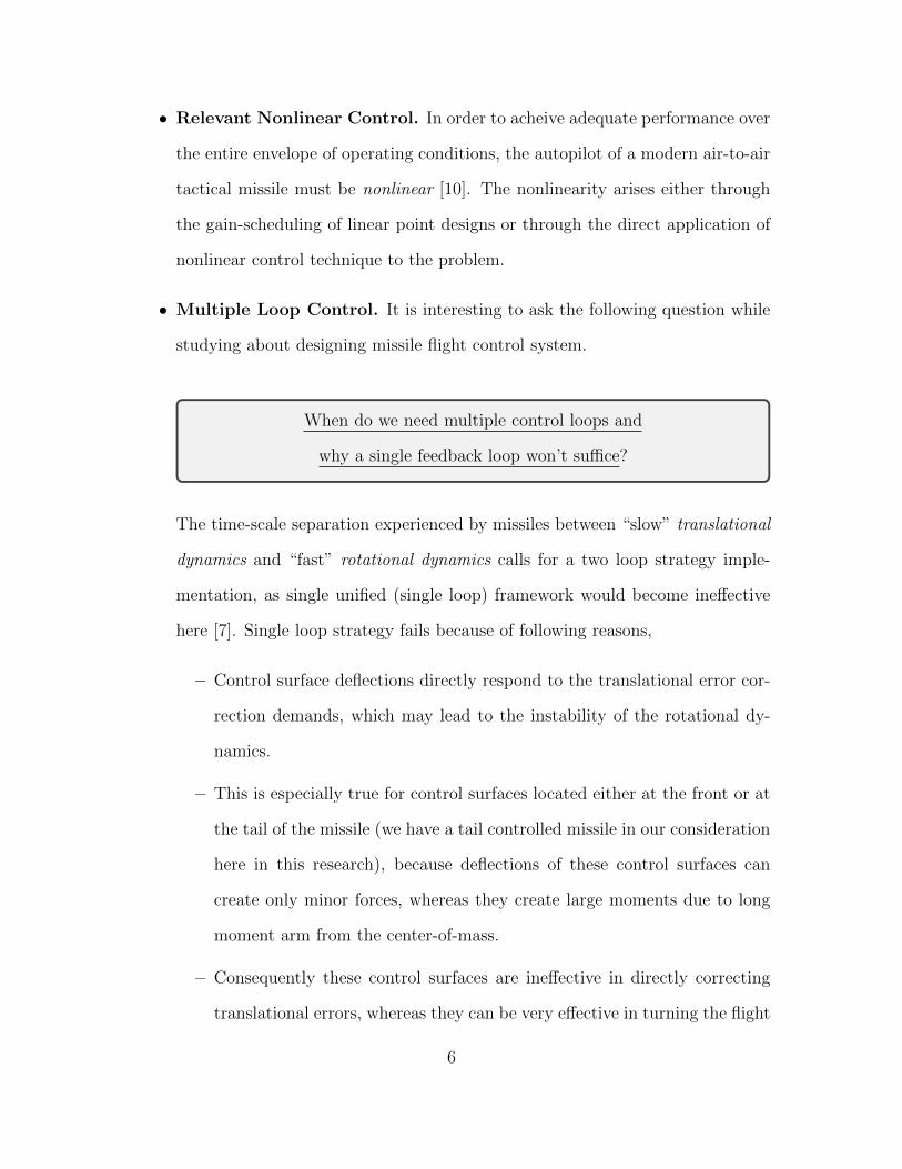
• Multiple Loop Control. It is interesting to ask the following question while
studying about designing missile flight control system.
When do we need multiple control loops and
why a single feedback loop won’t suffice?
The time-scale separation experienced by missiles between “slow” translational
dynamics and “fast” rotational dynamics calls for a two loop strategy imple-
mentation, as single unified (single loop) framework would become ineffective
here [7]. Single loop strategy fails because of following reasons,
– Control surface deflections directly respond to the translational error cor-
rection demands, which may lead to the instability of the rotational dy-
namics.
– This is especially true for control surfaces located either at the front or at
the tail of the missile (we have a tail controlled missile in our consideration
here in this research), because deflections of these control surfaces can
create only minor forces, whereas they create large moments due to long
moment arm from the center-of-mass.
– Consequently these control surfaces are ineffective in directly correcting
translational errors, whereas they can be very effective in turning the flight
6

vehicle.
Therefore, for a successful flight control system, the design must exploit the
time-scale separation that exists between translational and rotational motions
of the center-of-mass.
• Autopilot Innermost-Loop Control. A nonlinear controller with its gains
scheduled as function of different flight conditions is implemented here. Inner-
most loop is mainly for stabilizing the missile while helping the missile to follow
the commanded angular rates by issuing proper fin commands to the actuators.
Essentially innermost autopilot loop is meant for controlling angular rates here,
referred sometimes as Rate Loop.
• Autopilot Intermediate-Loop Control. Intermediate loop is mainly for
controlling the missile bank angle, angle of attack and sideslip angle while help-
ing the missile to follow the commanded bank angle which is generated by the
BTT Logic module.
• Outer-Loop Guidance Control. Within this thesis, various outer-loop guid-
ance control laws are examined. Usually referred as the Guidance Loop, this
will help the missile to steer towards the target (read it as position control loop).
Essentially this is also proportional controlled loop with gains determined by
the guidance laws.
1.3 Goals and Contributions
Miss distance of the target with respect to the missile was analyzed upon varying
various parameters of missile and the results are presented in this work and they agree
[1; 17; 16; 15; 33]. This research work will address and provide concrete answers to see
if the Kill Zone Estimation done using binary search algorithm correlates well with
7

the miss distance results presented in above mentioned papers. Missile parameters
such as initial altitude, initial mach and maximum missile acceleration are varied in
different sizes, one at a time and the variation of estimated kill zone is analyzed.
Before pursuing the study, it is instructive to acknowledge some simple ideas and
intuitions below which are answered in this research.
1.4 Contributions of Work: Questions to be Addressed
Within this thesis, the following fundamental questions are addressed. When
taken collectively, the answers offered below, and details within the thesis, represent
a useful contribution to researchers in the field.
Why should a hierarchical inner-outer loop control architecture be
used? Hierarchical inner-outer loop controllers are found across many industrial/-
commercial/military application areas (e.g. aircraft, spacecraft, robots, manufactur-
ing processes, etc.) where it is natural for slower (outer-loop generated) high-level
commands to be followed by a faster inner control loop that must deliver robust
performance (e.g. low frequency reference command following, low-frequency distur-
bance attenuation and high-frequency sensor noise attenuation) in the presence of
significant signal and system uncertainty. A well designed inner-loop can greatly sim-
plify outer-loop design. An excellent example of inner-outer loop architectures are
used in this missile-target application arena. Here, an autopilot (inner-loop)1 follows
commands generated from the guidance system (outer-loop). More substantively,
inner-outer loop control structures are used to tradeoff properties at distinct loop
breaking points (e.g. outputs/errors versus inputs/controls) [43], [44].
1Within an autopilot there is typically very critical lower-level actuator control inner-loops.
8

Inner-Loop Control What are typical inner-loop objectives? Typical inner-
loop objectives can be speed control; i.e. requiring the design of a angular speed
control system. Within this thesis, inner-loop control for our BTT missile specifically
refers to nonlinear gain scheduled autopilot.
What is a suitable inner-loop control structure? When is a classical
(decentralized) PI structure sufficient? When is a multivariable (central-
ized) structure essential? For many applications such as differential drive robotic
vehicle, a simple PI/PID (decentralized) control law with high frequency roll-off and
a command pre-filter suffices (see Chapters 3 and 6). Such an approach should work
when the plant is not too coupled and the design specifications are not too aggressive
relative to frequency dependent modeling uncertainty. A multivariable (centralized)
structure becomes essential when the plant is highly coupled such as the missile
control system considered within this thesis and the design specifications are very
aggressive (e.g. high bandwidth relative to coupling/uncertainty)[65].
What are the limitations on the bandwidth of the missile flight control
system? How does the presence of RHP zeros (nonminimum phase) and
RHP poles affect the closed loop bandwidth? The pitch up instability phe-
nomenon present in all tail controlled vehicles give rise to both RHP pole and RHP
zeros in system. While the unstable pole demands a minimum bandwidth to stabilize
the system, the nonminimum phase zero poses an upward limit on the maximum
bandwidth of the system. Thus going by the thumb rule, the bandwidth of a system
with RHP pole, ‘p’ and RHP zero, ‘z’ is given by following equation.
2 |p| ≤ Bandwidth ≤ |z|2
(1.1)
What is a suitable outer-loop control structure? When is a more com-
plex structure needed? Suppose that an inner-loop speed control system has been
9
designed. Suppose that it looks like as+a
. It then follows that if position is con-
cerned, then we have a system that looks like[
as(s+a)
]; i.e. there is an additional
integrator present. Given this, classical control (root locus) concepts [64] can be
used to motivate an outer-loop control structure Ko = g(s + z). In an effort to
attenuate the effect of high frequency sensor noise, one might introduce additional
roll-off; e.g. Ko = g(s+z)[
bs+b
]nwhere n = 2 or greater. (See work within Chapter 6)
1.5 Overview of Thesis
In this research, a MATLAB application is developed and used to evaluate the
performance of missile guidance and control systems. The program simulates and
uses MATLAB 3D Animation using VRML toolbox to display the missile-target air-
to-air engagement. The endgame portion of the engagement is of particular interest
whereby the target maneuvers causing the missile controls to saturate and possibly
induce instability [76]. The missile controls may saturate in the thin air found at
higher altitudes or when the actuator saturation limit is small. It would be desirablle
to visualize this phenomenon and quantify it and use the techniques in [41], [39], [34],
[45], [42] and [46] to prevent it. The simulation includes realistic missile and actuator
dynamics, various guidance systems (proportional, optimal and differential game), a
seeker navigation system model and various target models. The target represents a
simplified version of a high performance enemy aircraft. The three-degree-of-freedom
target is modeled with its acceleration limited to ±9 Gs, values tolerable to human
pilot.
10

Fig
ure
1.1:
Info
rmat
ion
Flo
wfo
rM
issi
le-T
arge
tE
nga
gem
ent.
11

Figure 1.1 illustrates how the above systems interact with one another, Each
subsystem is briefly discussed as follows:
Figure 1.2: Organization of MATLAB Program: 3 Modules.
Missile Dynamics. A set of nonlinear ordinary differential equations capturing aero-
dynamic, atmospheric and variable mass effects are used to model an EMRAAT BTT
missile. The model relates four controls (fin deflections - F1, F2, F3, F4) to the missile’s
coordinate velocities (Vmx, Vmy, Vmz) and its roll, pitch and yaw angles (φ, θ, ψ).
Actuator Dynamics. Each of the four missile fins is controlled by a servo-based
actuation system - modelled by a nonlinear underdamped system with position and
rate saturations.
Autopilot. Because of the inherent instabilities associated with missiles, stability
augmentation systems are essential. The autopilot provides the added stability and
ensures that acceleration commands from the guidance system are properly followed.
More precisely, the autopilot uses feedback to process the guidance commands and
deliver appropriately coordinated fin commands to the actuators.
Guidance System. The purpose of the guidance system is to issue appropriate
acceleration commands to the autopilot on the basis of target information obtained
12

from the seeker/navigation (target sensing) system.
Seeker/Navigation System. The seeker/navigation (target sensing) system gener-
ates target line-of-sight (LOS) rate information which is used by the guidance system.
Target Dynamics. Different models are used to reflect the maneuverability and
intelligence of the target. Each model has 3 degree of freedom.
The prime objective is to minimize the distance 1 between the missile and the
target within a limited time.
1.6 Organization of Thesis
The remainder of the thesis is organized as follows.
• Chapter 2 (page 16) presents an overview for a general 6DOF missile equations
of motions and 2nd order dynamics governing 4 missile fin actuators.
• Chapter 3 (page 55) describes the linearization routine followed in linearizing
the nonlinear missile plant. The ideas presented here include analysis of all dy-
namic flight modes of missile with respect to different flight parameters. This
chapter also provides a foundation for the work in Chapter 6 where both au-
topilot and plant analysis is done together.
• Chapter 4 (page 114) presents seeker dynamics and the 6DOF missile guidance
laws that helps the missile to intercept a maneuvering target. Three different
guidance laws are described.
1Miss distance is defined as the final range between missile and target, after the missile has tried
to intercept the target.
13

• Chapter 5 (page 129) describes 3DOF target modeling and its three different
maneuvering modes are discussed in detail.
• Chapter 6 (page 135) describes modeling and control issues for a Bank-To-Turn
(BTT) missile using a nonlinear autopilot. Linearization of missile autopilot
is discussed and this chapter serves as the basis for main control design. This
chapter contains the main work that was conducted in this research.
• Chapter 7 (page 184) describes the usage of different numerical integration
techniques. The chapter serves as the basis for selection of optimal step size for
numerical integration through engagement geometry analysis.
• Chapter 8 (page 196) describes the effect of different missile and target param-
eters on the final miss distance of a missile as described in [51] and [52]. The
chapter serves as the basis for Chapter 9, which is just an extension of chapter
8 ideas in a different perspective.
• Chapter 9 (page 219) describes the effect of different missile and target param-
eters on the estimated Kill zone of a missile using binary search algorithm.
• Chapter 10 (page 235) describes modeling and animating the entire missile-
target engagement using VRML toolbox of MATLAB. 3D animation results
using VRML toolbox and initial graphical user interface development are dis-
cussed.
• Chapter 11 (page 248) summarizes the thesis and presents directions for future
missile research. While much has been accomplished in this thesis, lots remains
to be done.
• Appendix A (page 258) contains C program implementation of Binary Search
algorithm to estimate kill zone. Also MATLAB files to plot the kill zone is
14

included in this section.
• Appendix B (page 264) contains MATLAB ‘m’ files used in this thesis for plot-
ting linearized plant and autopilot analysis plots.
1.7 Summary and Conclusions
In this chapter, we provided an overview of the work presented in this thesis and
the major contributions. A central contribution of the thesis is an improved autopilot
design with animation to visualize the missile target engagement and detailed Kill
Zone & Miss Distance analysis to explore the complexities involved in missile-target
engagement.
15

Chapter 2
MISSILE & ACTUATOR DYNAMICS
2.1 Introduction and Overview
In this chapter the six degree-of-freedom nonlinear missile dynamics are described.
Also described are the nonlinear fin actuator dynamics. Section 2.2 describes the ref-
erence frames used to develop the missile dynamics. Section 2.3 describes the effect
of fuel loss. Section 2.4 describes the aerodynamic relationships, i.e. the effects due
to the static and dynamic fluid properties of the atmosphere - accounted for via the
dynamic pressure, Mach number and stability derivatives. Section 2.5 contains the
equations of motion for the missile and Section 2.6 describes the nonlinear actua-
tor dynamics. Finally Section 2.7 summarizes the chapter and concludes the items
explained in this chapter.
2.2 Inertial, Vehicle and Body Frames
In this section three reference frames are described. A perspective, or reference
frames, can be selected so that the dynamics within them can be described by rela-
tively simple equations. The overall system can then be described by simply trans-
forming the equations from one reference frame to another. Reference frames used
in missile dynamics analysis include: (1) Inertial Frame, (2) Vehicle Relative Frame
and (3) the Body Frame. Introducing these reference frames significantly simplifies
the equations of motion for the missile.
16

2.2.1 Inertial Frame
Inertial Frame is a stationary coordinate system used to describe the motion of
all objects within it. Throughout the thesis and in the program, the origin of this
frame (0, 0, 0)i 1 is located at sea level directly below the missile initial launch point
as shown in the Figure 2.1. This assumption is valid and typical for short range
missions. It is not valid, for example, in long range Inter-Continental Ballistic Missile
(ICBM) applications [62]. Given the above convention, the missile’s launch (time
zero) center of gravity, denoted by CG0 is located by the inertial point:
Figure 2.1: Local Inertial Frame with missile and target flight paths
Smi def
= (Smx, Smy, Smz)i (2.1)
Its inertial velocity is denoted by
Vmi def
= (Vmx, Vmy, Vmz)i (2.2)
The missile’s inertial angular velocity is denoted by
1The superscript i will be used to denote a coordinate with respect to the inertial frame
17

Ωmi def
= (Ωmx,Ωmy,Ωmz)i (2.3)
Similarly, the target is located by the inertial point:
Sti def
= (Stx, Sty, Stz)i (2.4)
The target’s inertial velocity is denoted by
Vti def
= (Vtx, Vty, Vtz)i (2.5)
Also shown in Figure 2.1 are typical missile and target flight paths.
2.2.2 Vehicle Frame
Often it is convenient to use the missile’s (time zero) center-of-gravity, CGo as
the origin and this motivates the so-called vehicle frame. This is a nonstationary
coordinate system used to measure the relative distance between the missile and
target, its origin is at the missile’s (time zero) center-of-gravity, CGo. This is a right-
handed coordinate system centered at CGo with axes denoted (Xv, Y v, Zv) which
remain parallel to their inertial counterparts (X i, Y i, Zi). The vehicle frame can be
visualized as shown in Figure 2.2.
Figure 2.2: Visualization of Inertial and Vehicle Frames
18

2.2.3 Body Frame
A coordinate system is needed to conveniently define the missiles physical geom-
etry as well as sum all forces and moments acting on the missile. This motivates
the body frame. This is a right-handed coordinate system centered at missile’s (time
zero) center-of-gravity, CGo. Its axes are denoted (Xb, Y b, Zb), where Xb emerges
from the missile’s nose is a forward axis and Y b is a starboard axis. The body frame
can be visualized as shown in Figure 2.3.
Figure 2.3: Visualization of Body Axes and Velocities
Body Axis Velocities.
We define the missile’s body axis velocities (U, V, W) to be the components of
the missile’s inertial velocity Vmi along the body axes (Xb, Y b, Zb). The body axis
velocities can be visualized as shown in Figure 2.3.
Body Axis Angular Velocities.
We define the missile’s body axis angular velocities (P, Q, R) to be the components
of the missile’s inertial angular velocity Ωmi along the body axes (Xb, Y b, Zb). These
body axis angular velocities can be visualized as shown in Figure 2.3.
Euler Angles and Missile Attitude.
To precisely specify the orientation(attitude) of the missile in inertial space, it is
19

convenient (and convention) to introduce the so-called Euler angles (φ, θ, ψ). To
precisely define these angles, consider the vehicle and body axes systems shown in
Figure 2.4.
Figure 2.4: Visualization of Euler Angles
To define the Euler angles we proceed as follows. Let N1 denote the projection of
Xb onto the XvY v (horizontal) plane 2:
N1def= PXvY vX
b (2.6)
where PXvY v denotes a projection operator. The missile pitch angle or pitch
attitude is then defined as the angle from N1 to Xb measured in the vertical N1Xb
plane:
θdef= ∠N1X
b (2.7)
2Recall that the XvY v plane is parallel to the XiY i plane. See Figure 2.2.
20
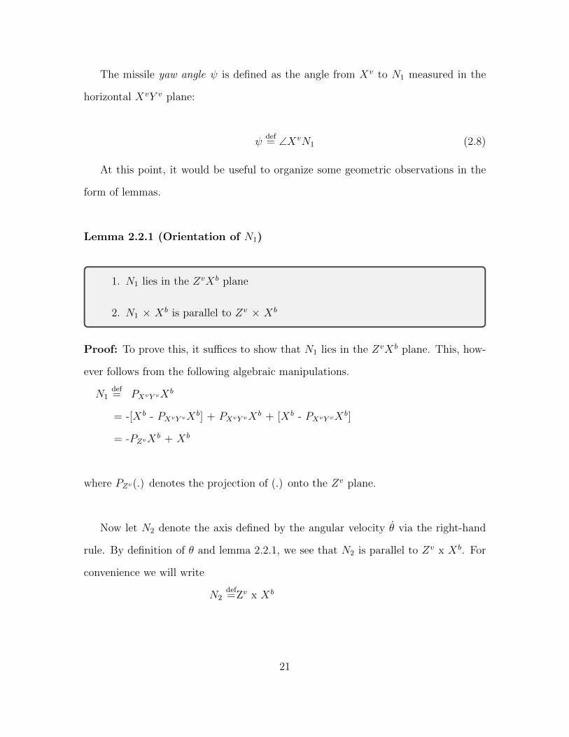
The missile yaw angle ψ is defined as the angle from Xv to N1 measured in the
horizontal XvY v plane:
ψdef= ∠XvN1 (2.8)
At this point, it would be useful to organize some geometric observations in the
form of lemmas.
Lemma 2.2.1 (Orientation of N1)
1. N1 lies in the ZvXb plane
2. N1 × Xb is parallel to Zv × Xb
Proof: To prove this, it suffices to show that N1 lies in the ZvXb plane. This, how-
ever follows from the following algebraic manipulations.
N1def= PXvY vX
b
= -[Xb - PXvY vXb] + PXvY vX
b + [Xb - PXvY vXb]
= -PZvXb + Xb
where PZv(.) denotes the projection of (.) onto the Zv plane.
Now let N2 denote the axis defined by the angular velocity θ via the right-hand
rule. By definition of θ and lemma 2.2.1, we see that N2 is parallel to Zv x Xb. For
convenience we will write
N2def=Zv x Xb
21

Given this, we make the following observation:
Lemma 2.2.2 (Orientation of N2)
1. N2 lies in the Y bZb plane
Proof: If one lets Zv = α1Xb + α2Y
b + α3Zb, then the result follows from the
following equality:
N2 = Zv x Xb = [α1Xb + α2Y
b + α3Zb] x Xb
= α2Yb x Xb + α3Z
b x Xb
= β1Zb + β2Y
b
for some scalars β1, β2.
It should be noted that the Y bZb plane, in general, need not be vertical. Given
lemma 2.2.2, one should justifiably define the missile roll angle or roll attitude to be
the angle from N2 to Y b measured in the Y bZb plane:
φdef= ∠N2Y
b (2.9)
To relate the Euler rates (φ, θ, ψ) to the body rates (P, Q, R), it is convenient to
define N3 to be the projection of Zv onto the Y bZb plane:
N3def= PY bZbZ
v (2.10)
Now we make the following important geometric observations.
22

Lemma 2.2.3 (Orientation of N1, N2 and N3)
1. N1 ⊥N2, N2 ⊥ N3, N1 not ⊥ N3
2. ∠ N2Yb = ∠ N3Z
b = φ
3. N3 lies in the ZvXb plane
4. ∠ ZvN3 = ∠ N1Xb = θ
Proof:
(1) Since
N2 = Zv x Xb = Zv x [PXvY vXb + Xb - PXvY vX
b]
= Zv x [N1 + PZvXb]
= Zv x N1
it follows that N1 and N2 are orthogonal. Similarly, since
N2 = Zv x Xb = [PY bZbZv + Zv - PY bZbZ
v] x Xb
= [N3 + PXbZv] x Xb
= N3 x Xb
It follows that N2 and N3 are orthogonal. Also, since N1 = PXvY vXb and N3 =
PY bZbZv, it follows that N1 and N3 need not to be orthogonal.
(2) From lemma 2.2.2 N2 lies in the Y bZb plane. N3 lies in this plane by the
23

definition. Since N2 and N3 are orthogonal and both lie in the Y bZb plane, it follows
from Figure 2.5 that
∠ N2Yb = ∠ N3Z
b = φ
Figure 2.5: Visualization of N2 and N3 in Y bZb plane.
(3) Since N3 = PY bZbZv = Zv - [Zv - PY bZbZ
v] = Zv - PXbZv
it follows that N3 lies in the ZvXb plane.
(4) Now recall from lemma 2.2.1 that N1 lies in the Zv x Xb plane. Since N3 does
also, it follows from Figure 2.6 that
∠ ZvN3 = ∠ N1Xb = θ
24
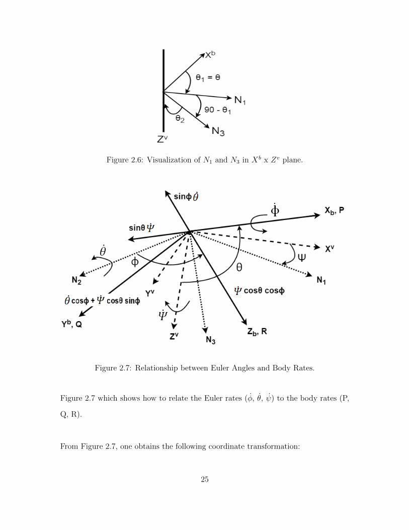
Figure 2.6: Visualization of N1 and N3 in Xb x Zv plane.
Figure 2.7: Relationship between Euler Angles and Body Rates.
Figure 2.7 which shows how to relate the Euler rates (φ, θ, ψ) to the body rates (P,
Q, R).
From Figure 2.7, one obtains the following coordinate transformation:
25

P
Q
R
=
1 0 − sin(θ)
0 cos(φ) cos(θ) sin(φ)
0 − sin(φ) cos(θ) cos(φ)
φ
θ
ψ
(2.11)
from which one obtains:
φ
θ
ψ
=
1 sin(φ) tan(θ) cos(φ) tan(θ)
0 cos(φ) − sin(φ)
0 sin(φ) sec(θ) cos(φ) sec(θ)
P
Q
R
(2.12)
2.3 Thrust Profile and Variable-Mass Dynamics
Loss of mass through fuel comsumption influence missile dynamics and must be
accounted for in a realistic manner. Mass loss during flight causes the CG to move
forward with respect to the CG0, because the seeker is located in the forward part of
the missile. The rate of mass loss will also vary with time due to the missile being
modeled with variable thrust. A two-stage thrust profile is used in this simulation. A
large initial thrust is needed to free the missile from the launching aircraft. A second
level of thrust allows the missile to approach the target while remaining within its
designed capabilities. The two thrust levels are as follows:
Th1 = 9250 lbs (2.13)
Th2 = 2140 lbs (2.14)
as shown in the Figure 2.8.
26

Figure 2.8: Missile Two-Stage Thrust Profile
The thrust profile is a piecewise linear function of time. All variable-mass effects
are modeled as piece-wise linear time functions. Small time-constant exponential
fucntions are used to smooth the piecewise connected thrust profile at the transition
points. A more precise description of the thrust profile is given in Table 2.1. Tchange
= 0.025 sec, is equal to half the time required to make a thrust transition. It is chosen
to be much smaller than the Th1 time interval, which is equal to 0.6 sec. The time
constant τp (equal to 0.01 sec) is chosen to be at least 5 times smaller than 2Tchange.
27

t0 = = 0.000 sec
t1 = Tchange = 0.025 sec
t2 = t1 + Tchange = 0.050 sec
t3 = = 0.600 sec
t4 = t3 + Tchange = 0.625 sec
t5 = t4 + Tchange = 0.650 sec
t6 = = 6.090 sec
t7 = t6 + Tchange = 6.115 sec
t8 = t7 + Tchange = 6.140 sec
Modified Thrust. The caveit of using the above thrust profile is it may lead to
missile being travelling at say Mach 7 at an altitude of 40 kft which is bad. The missile
can’t travel at such higher mach values given its fuel, aerodynamics and design. So
to avoid the above confusion, it is suggested to have the following modified thrust
profile, which is obtained through multiplying scaled air density component (ρ) in old
thrust profile. Air gets thinner as we go up and if that is modelled along with this
thrust profile as below, then missile will always stay within its specified mach value.
This change is discussed in [6] but not present in simulation environments done by
[2] & [5]. ρsl is a constant (air density at sea level) and defined as 0.0024 slugft3
.
Thrustnew = Thiρ
ρsl(2.15)
where i = 1,2 respectively. By assumption, the time-derivative of the missile’s
mass and moments of inertia are directly proportional to the missile impulse time-
derivative, where impulse is given as the time integral of thrust:
28
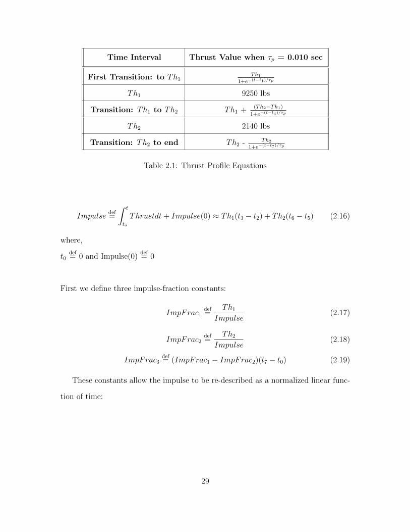
Time Interval Thrust Value when τp = 0.010 sec
First Transition: to Th1Th1
1+e−(t−t1)/τp
Th1 9250 lbs
Transition: Th1 to Th2 Th1 + (Th2−Th1)
1+e−(t−t4)/τp
Th2 2140 lbs
Transition: Th2 to end Th2 - Th21+e−(t−t7)/τp
Table 2.1: Thrust Profile Equations
Impulsedef=
∫ t
to
Thrustdt+ Impulse(0) ≈ Th1(t3 − t2) + Th2(t6 − t5) (2.16)
where,
t0def= 0 and Impulse(0)
def= 0
First we define three impulse-fraction constants:
ImpFrac1def=
Th1
Impulse(2.17)
ImpFrac2def=
Th2
Impulse(2.18)
ImpFrac3def= (ImpFrac1 − ImpFrac2)(t7 − t0) (2.19)
These constants allow the impulse to be re-described as a normalized linear func-
tion of time:
29

ImpNorm =
0 : t < t2
ImpFrac1 t : t2 < t < t3
ImpFrac2 t+ ImpFrac3 : t5 < t < t6
1 : t6 < t
(2.20)
Missile mass can now be represented by a time function:
m(t) = m0 − ImpNorm(t) dm (2.21)
where m0 = 5.75 slug is the missile’s time-zero mass and dm = 2.2689 slug is
defined so where, [ImpNorm(t8 - t0) dm] is the total mass lost from t0 to t8. The
missile’s principal moments of inertia are similarly defined:
Ixx(t) = Ixxo − ImpNorm(t) dIxx (2.22)
Iyy(t) = Iyyo − ImpNorm(t) dIyy (2.23)
Izz(t) = Izzo − ImpNorm(t) dIzz (2.24)
where time-zero moments and impulse change in moments of inertia are defined
in Table 2.2.
The CG is located along the body frame positive X-axis using:
XCG(t) = ImpNorm(t) dCG (2.25)
Figure 2.9 shows the orientation of the CG to the missile body frame.
30

Time-Zero Missile Inertial
Moment (slug-ft2)
Impulse Change in Moment
of Inertia (slug-ft2)
Ixxo = 0.34 dIxx = 0.11
Iyyo = 34.1 dIyy = 6.94
Izzo = 34.1 dIzz = 6.90
Table 2.2: Missile’s Time-Zero Mass and Moment of Inertia
Figure 2.9: Visualization of CG0 and Vb
Ixx, Iyy, Izz, XCG, their derivatives and mass denoted by m(t), are then included
in the derivation of the missile dynamic equations. The time-derivative of Mass is
accounted for in the missile thrust term.
Maximum Missile Acceleration Calculation. By Newton’s law, F = ma, we
understand that the acceleration varies inversely with respect to the mass. Thus
missile will reach its maximum acceleration when maximum fuel mass is lost during
its flight. Missile acceleration is measured in terms of G-force here. When the missile
fligh time t > t6, the ImpNorm would be 1 and missile will have the least mass. Going
by the Equation 2.21, we calculate the maximum mass lost as follows.
31

MaximumMassLost = ImpNorm(t) dm
= 1 ∗ 2.2689
= 2.2689 slugs
Thus the remaining missile mass is given by,
RemainingMass = m0 −MaximumMassLost
= 5.7500− 2.2689
= 3.4811 slugs = 50.8028 kg = 498.205N
Maximum Thrust is given as = 9250 lbs = 4195.729 kg = 41146.04591 N. The “g”
force is calculated as follows,
Gforce =Thrust
Weight
=Thrust inN
mass in kg ∗ 9.8ms−2
=Thrust inN
Weight inN
Thus the maximum G force will occur when the thrust is max and weight is
minimum.
MaximumGforce =Maximum Thrust
Minimum Weight
=41146.04591N
495.205N
= 82.58
Thus the BTT missile in our considered can maximum pull up to 82.58 g’s with
its capabilities while trying to intercept a target. 82.58 g is really a considerable
acceleration advantage over the target which is limited to maximum ± 9g, which a
human pilot can endure.
32

2.4 Missile Aerodynamics
During the missile’s flight through the atmosphere, it will experience aerodynamic
forces, Fw and moments Gw [49]. The amount of lift generated and drag that must
be overcome are greatly influenced by the missile’s orientation with respect to its
velocity vector, speed and the local dynamic air pressure.
If one defines the missile’s body frame inertial speed, Vb as:
Vbdef=√
(U2 + V 2 +W 2) (2.26)
then the dynamic pressure Qdp is a function of the local air density ρ and is given by:
Qdp = 0.5ρV 2b (2.27)
A critical parameter in this work is Mach Number. Mach number is defined as follows:
Machdef=
VbSOS
(2.28)
where SOS is the local speed-of-sound.
For missile velocity Vb less than the local SOS, the missile motion produces com-
pression waves which radiate away from the missile in all directions. The wave motion
in advance of the missile starts the local air molecules in motion, in a manner such
that they flow smoothly out of the path of the missile. This is known as the sub-sonic
flight and the missile lift, drag and sideforce characteristics depend on the smooth flow
of the atmosphere over the surface area of the missile. For missile velocity Vb greater
than the local SOS, the air molecules recieve no advance warning of the approaching
missile and are forced rapidly out of the way at speeds greater than the local SOS,
33

creating a shock wave [57]. This is known as supersonic flight. The lift, drag and
sideforce properties of the missile are significantly changed from those properties at
sub-sonic flight.
SOS and ρ are in turn functions of the missile’s inertial altitude Smzi and are
modeled using equations fitted to a set of tabulated data [57], [58]. The tabulated data
contains results of extensive wind-tunnel tests. SOS and ρ decrease with increasing
altitude. More precisely, SOS varies as temperature and ρ varies as temperature
(below 36088 ft) or altitude (above 36088 ft, geopotential height).
2.4.1 Stability and Control Derivatives
In order to express the external body frame forces (Fx, Fy, Fz) and body frame
moments (L, M, N) in terms of the aerodynamic variables (α, β), aerodynamic pa-
rameter (Mach) and the controls (δp, δq, δr), it is convention to introduce the stability
derivatives in Table 2.3 and the control derivatives in Table 2.4. These coefficients
represent the partial derivatives of body frame forces (Fx, Fy, Fz) with respect to
body linear velocities (U, V, W) and body frame moments (L, M, N) with respect to
body frame angular velocities (P, Q, R). Stability derivatives are interpolated from
aerodynamic coefficient arrays created using empirical values measured during the ac-
tual missile wind-tunnel tests. Tables are used becuase of the complex dependence on
Mach number, angle of attack and sideslip angles. This simulation still uses 15 aero-
dynamic coefficients which are interpolated using Mach, α, β&δq. Their parameter
dependence is indicated in Table 2.3 and Table 2.4.
34

Aero Coefficients Quantifies Depends on
CD Drag from Pitch Fin Deflection δq, Mach-1, α-1
CDT Base Drag due to Mach Mach-2
CLβ Roll Moment from Sideslip Mach-1, α-1
CLP Roll Damping Moment - Pitch rate Mach-1, α-3
CMα Pitch Moment from Angle of Attack Mach-1, α-4
CMq Pitch Moment from Pitch Fin Deflection Mach-2, α-3
CNα Lift due to Mach Mach-1
CNβ Yaw Moment from Sideslip Mach-1, α-1
CNR Yaw Damping Moment - Yaw Rate Mach-2, β-2
CYβ Side Force from Sideslip Mach-1, α-1
Table 2.3: Stability Derivatives and Parameter Dependence
Aero Coefficients Quantifies Depends on
CLδp Roll Moment from Roll Fin Deflection Mach-1, α-1
CMδqPitch Moment from Pitch Fin Deflection Mach-1, α-2
CNδq Lift from Pitch Fin Deflection Mach-1, α-2
CNδr Yaw Moment from Yaw Fin Deflection Mach-1, β-1
CYδr Side Force from Yaw Fin Deflection Mach-1, β-1
Table 2.4: Control Derivatives and Parameter Dependence
Polynomial Fit Data Models and Dynamic Implications
Stability & Control derivatives were studied for their complex dependencies on flight
parameters. Polynomial fitting of these Stability & Control derivatives will cut down
35

the computation time of simulation by several times as this will avoid matrix parsing
of aerodynamic look up tables using interpolation.
1020
3040
50
1
2
3
4
5
−2
−1.5
−1
−0.5
delQ
CD − Linear Interpolation
alpha 1
CD
Figure 2.10: CD - Drag from Pitch Fin Deflection - depends on δq, Mach-1, α-1
1 2 3 4 5 6 7 8 90.04
0.06
0.08
0.1
0.12
0.14
0.16CDT
Mach 2
CD
T
Figure 2.11: CDT - Base Drag due to Mach-2
36

02
46
810
0
2
4
6−0.4
−0.3
−0.2
−0.1
0
0.1
Mach 1
CLBeta − Linear Interpolation
alpha 1
CLB
eta
Figure 2.12: CLβ - Roll Moment from Sideslip - depends on Mach-1, α-1
02
46
810
0
2
4
60.04
0.06
0.08
0.1
0.12
0.14
0.16
Mach 1
CLdelP − Linear Interpolation
alpha 1
CLd
elP
Figure 2.13: CLδp - Roll Moment from Roll Fin Deflection - depends on Mach-1, α-1
37
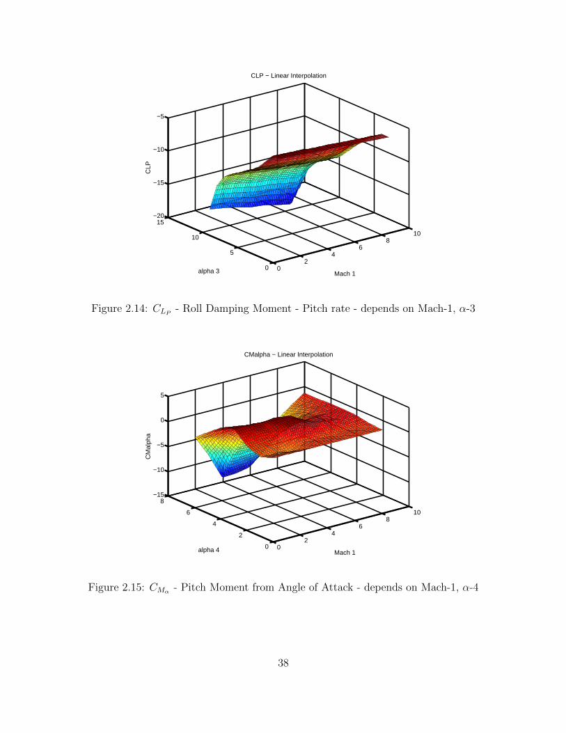
02
46
810
0
5
10
15−20
−15
−10
−5
Mach 1
CLP − Linear Interpolation
alpha 3
CLP
Figure 2.14: CLP - Roll Damping Moment - Pitch rate - depends on Mach-1, α-3
02
46
810
0
2
4
6
8−15
−10
−5
0
5
Mach 1
CMalpha − Linear Interpolation
alpha 4
CM
alph
a
Figure 2.15: CMα - Pitch Moment from Angle of Attack - depends on Mach-1, α-4
38

02
46
810
0
5
10
15−1.2
−1
−0.8
−0.6
−0.4
−0.2
Mach 1
CMdelQ − Linear Interpolation
alpha 2
CM
delQ
Figure 2.16: CMδq- Pitch Moment from Pitch Fin Deflection - depends on Mach-1,
α-2
02
46
810
0
5
10
15−14
−12
−10
−8
−6
−4
−2
Mach 2
CMQ − Linear Interpolation
alpha 3
CM
Q
Figure 2.17: CMq - Pitch Moment from Pitch Fin Deflection - depends on Mach-2,
α-3
39

1 2 3 4 5 6 7 8 9−0.7
−0.65
−0.6
−0.55
−0.5
−0.45
−0.4
−0.35CNalpha Plot
Mach 1
CN
alph
a
Figure 2.18: CNα - Lift due to Mach-1
02
46
810
0
2
4
6−0.5
0
0.5
1
1.5
Mach 1
CNbeta − Linear Interpolation
alpha 1
CN
beta
Figure 2.19: CNβ - Yaw Moment from Sideslip - depends on Mach-1, α-1
40
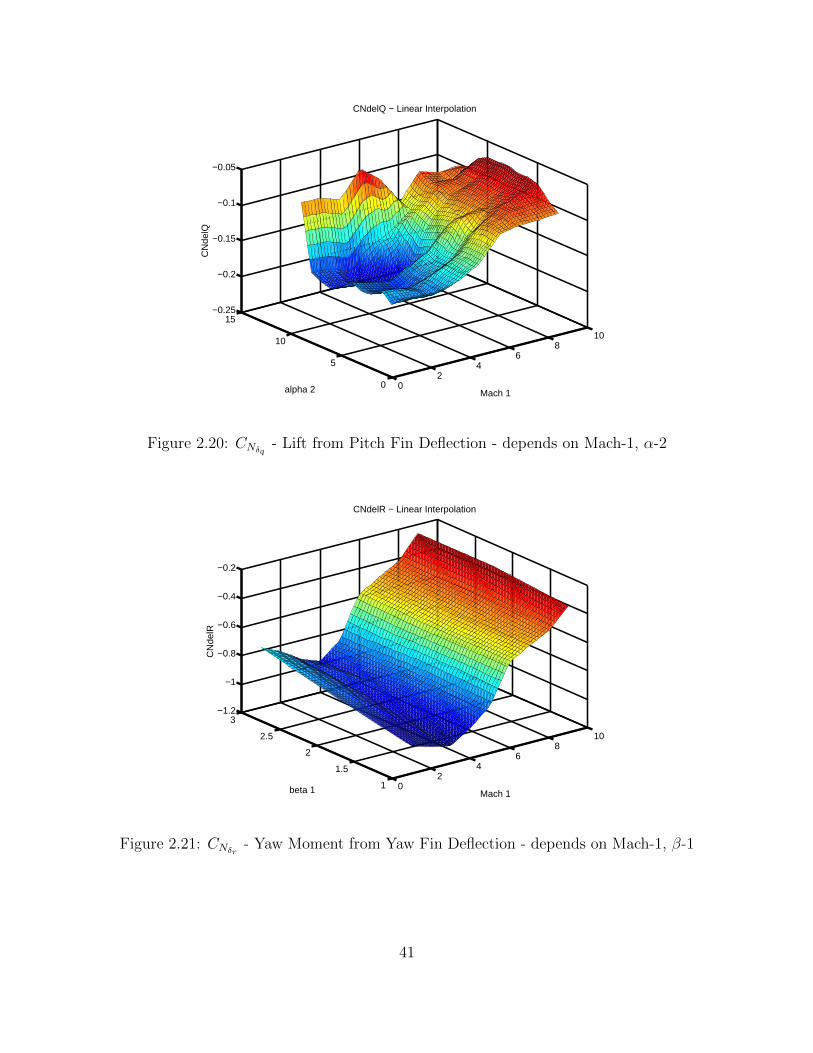
02
46
810
0
5
10
15−0.25
−0.2
−0.15
−0.1
−0.05
Mach 1
CNdelQ − Linear Interpolation
alpha 2
CN
delQ
Figure 2.20: CNδq - Lift from Pitch Fin Deflection - depends on Mach-1, α-2
02
46
810
1
1.5
2
2.5
3−1.2
−1
−0.8
−0.6
−0.4
−0.2
Mach 1
CNdelR − Linear Interpolation
beta 1
CN
delR
Figure 2.21: CNδr - Yaw Moment from Yaw Fin Deflection - depends on Mach-1, β-1
41

02
46
810
1
2
3
4−14
−12
−10
−8
−6
−4
−2
Mach 2
CNR − Linear Interpolation
beta 2
CN
R
Figure 2.22: CNR - Yaw Damping Moment - Yaw Rate - depends on Mach-2, β-2
02
46
810
0
2
4
6−0.35
−0.3
−0.25
−0.2
−0.15
−0.1
−0.05
0
Mach 1
CYbeta − Linear Interpolation
alpha 1
CY
beta
Figure 2.23: CYβ - Side Force from Sideslip - depends on Mach-1, α-1
42

02
46
810
1
1.5
2
2.5
30
0.05
0.1
0.15
0.2
Mach 1
CYdelR − Linear Interpolation
beta 1
CY
delR
Figure 2.24: CYδr - Side Force from Yaw Fin Deflection - depends on Mach-1, β-1
02
46
810
0
2
4
6−6
−5
−4
−3
−2
−1
0
1
Mach 1
CLBeta / CLdelP − Linear Interpolation
alpha 1
CLB
eta
/ CLd
elP
Figure 2.25: Scheduled Gain
43

2.4.2 Aerodynamic (Wind) Frame
The aerodynamic frame is defined so as to relate the missile body frame veloc-
ity and orientation to the external aerodynamic forces and moments. The stability
and control derivatives are dependent on missile body rate information. The body
frame linear velocities are transformed into the aerodynamic frame by the following
equations.
Figure 2.26: Aerodynamic Force, Body Velocity and Aerodynamic Angles
Figure 2.26 shows the aerodynamic force Fw = (X, Y, Z)w, body velocity Vm and
44

aerodynamic angles - α, β defined below. Velocity of the missile in wind frame is
given by:
Vmw = (Vb, 0, 0)w (2.29)
Figure 2.27: Visualization of Sideslip Angle, β
Figure 2.28: Visualization of Angle of Attack, α
The orientation of the wind frame will now be discussed. The wind frame has its
origin at the missile center of gravity CG0, with Xw in the plane defined by Xw and
Y b as shown in the Figure 2.28. Zw is defined to be orthogonal to ~U + ~W in the
XbZb plane as shown in Figure 2.27. We now define two key aerodynamic variables:
(1) Angle of Attack α and (2) Sideslip Angle β. These quantities are defined in terms
of the body axis velocities (U, V, W) as follows. The Angle of Attack, denoted by α
is defined as shown in Figure 2.12 as the angle from Zb to Zw, i.e.
45

αdef= ∠ZbZw (2.30)
From figure 2.28, it also follows that
αdef= tan−1W
U(2.31)
The Sideslip Angle, denoted by β is defined as the angle from ~U + ~W to ~U + ~V
+ ~W , measured in the plane formed by ~U + ~W and Y b: The Sideslip Angle, denoted
by β is defined as shown in Figure 2.27 as the angle from Y b to Y w, i.e.
βdef= ∠Y bY w (2.32)
From Figure 2.27, it also follows that
βdef= tan−1 V√
(U2 +W 2)(2.33)
2.4.3 Force and Moment Coefficients
Stability derivatives are multiplied with dynamic parameter values to form body
frame force coefficients and body frame coefficients. Figure 2.29 [59] shows the aero-
dynamic forces (Fx, Fy, Fz), moments (L, M, N), body linear velocities (U, V, W)
and body angular velocities (P, Q, R). Their notation is defined in the Table 2.5.
46

Direction/Rotation Velocity Forces & Moments Distances
Forward U X = Fx x
Side V Y = Fy y
Vertical W Z = Fz z
Roll P L
Pitch Q M
Yaw R N
Table 2.5: Body Frame Force and Moment Notation
Figure 2.29: Body Frame Axis System and Notation
47

The symbols δp, δq, δr are equivalent to aileron, elevator and rudder deflections
for an aircraft. They are related to the actual fin deflections via an Integrated Logic
for Air-to-Air Technology (ILAAT) demixer [48].
The drag, side force and lift coefficients are:
CX = CD + CDT (2.34)
CY = CYββ + CYδr δr (2.35)
CZ = CNαα + CNδq δq (2.36)
and the roll, pitch and yaw moment coefficients are
CL = CLδpδp + CLPPL2V + CLββ (2.37)
CM = CMδqδq + CMQ
QL2V + CMαα (2.38)
CN = CNδr δr + CNRRL2V + CNββ (2.39)
where
L2Vdef=Lref
2Vb (2.40)
Lref = 0.625 (ft) is an effective reference missile length used to describe moments
about CG. CMα determines whether the airframe is statically stable [62]. A missile
is statically stable if it returns to its equilibrium point after encountering a small
disturbance [58].
48
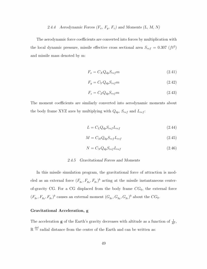
2.4.4 Aerodynamic Forces (Fx, Fy, Fz) and Moments (L, M, N)
The aerodynamic force coefficients are converted into forces by multiplication with
the local dynamic pressure, missile effective cross sectional area Sref = 0.307 (ft2)
and missile mass denoted by m:
Fx = CXQdpSrefm (2.41)
Fy = CYQdpSrefm (2.42)
Fz = CZQdpSrefm (2.43)
The moment coefficients are similarly converted into aerodynamic moments about
the body frame XYZ axes by multiplying with Qdp, Sref and Lref :
L = CLQdpSrefLref (2.44)
M = CMQdpSrefLref (2.45)
N = CNQdpSrefLref (2.46)
2.4.5 Gravitational Forces and Moments
In this missile simulation program, the gravitational force of attraction is mod-
eled as an external force (Fgx , Fgy , Fgz)b acting at the missile instantaneous center-
of-gravity CG. For a CG displaced from the body frame CG0, the external force
(Fgx , Fgy , Fgz)b causes an external moment (Ggx , Ggy , Ggz)
b about the CG0.
Gravitational Acceleration, g
The acceleration g of the Earth’s gravity decreases with altitude as a function of 1R2 ,
Rdef= radial distance from the center of the Earth and can be written as:
49

g = g0
√R0
R0 + hi(2.47)
where
hidef= the inertial altitude of missile = (Sz)
i
R0def= sea-level radius of Earth = 20,903,264 ft
g0def= sea-level value for gravity = 32.174 ft
sec2
Gravitational Acceleration
For the missile-target engagement, g is modeled as an inertial acceleration (Agx , Agy , Agz)i
= [0, 0, g]i and when transformed into the body frame is denoted as (Agx , Agy , Agz)b.
Gravitational Force and Moment
The external gravitational force (Fgx , Fgy , Fgz)b acting on the missile CG is given by:
(Fgx , Fgy , Fgz)b = m(Agx , Agy , Agz)
b (2.48)
and therefore the components are
Fgx = mAgx (2.49)
Fgy = mAgy (2.50)
Fgz = mAgz (2.51)
An external gravitational moment, (Ggx , Ggy , Ggz)b results because the force (Fgx , Fgy , Fgz)
b
is applied at the missile CG, which is displaced from body frame origin by a distance
(Scx , Scy , Scz)b. The moment equation is given by:
50

(Ggx , Ggy , Ggz)b = (Scx , Scy , Scz)
b × (Fgx , Fgy , Fgz)b (2.52)
The CG motion is confined along the body frame X-axis for this model, the last
equation expands as:
Ggx = 0 (2.53)
Ggy = −ScxFgz (2.54)
Ggz = ScxFgy (2.55)
2.5 Equations of Motion for the Missile
A complete set of 6DOF nonlinear equations can be described by summing all
external forces and moments, (external forces being defined as the aerodynamic and
gravitational forces and moments), acting on the missile and setting them equal to
the forces and moments due to the missile inertial acceleration. Inertial and external
components are indicated by i and e subscripts respectively.
Translational Dynamics
Inertial accelerations expresses in body frame (X, Y, Z)b are:
Aix = U +QW −RV + XCG −XCG(Q2 +R2) (2.56)
Aiy = V +RU −RW + 2RXCG −XCG(PQ+ R) (2.57)
Aiz = W + PV −QU + 2QXCG −XCG(PR− Q) (2.58)
where XCG(t) is given by the Equation (2.25).
The second derivative of XCG is retained to model effects during rocket thrust
transients. XCG is defined as the distance the instantaneous missile CG is displaced
51

from the body frame origin CG0, XCG = Scx .
These inertial accelerations (Aix, Aiy, Aiz) are set equal to the accelerations caused
by external forces (Aex, Aey, Aez), which include: (1) the aerodynamic forces, (2)
rocket thrust and (3) gravity transformed into the body frame:
Aex =Fx
Mass+ Fgx
b +Thrust
Mass(2.59)
Aey =Fy
Mass+ Fgy
b (2.60)
Aez =Fz
Mass+ Fgz
b (2.61)
where (Fx, Fy, Fz) are specified by equations (2.41) - (2.43), thrust is specified by
equations (2.13) - (2.14), m is specified by the equation (2.21) and (Fgx , Fgy , Fgz)b are
given in equations (2.49) - (2.51).
Rotational Dynamics
Inertial moments about the body frame XYZ axes are described by:
Li = P Ixx + P Ixx +QR(Izz − Iyy) (2.62)
Mi = QIyy +QIyy +RP (Ixx − Izz) (2.63)
Ni = RIzz +RIzz + PQ(Iyy − Ixx) (2.64)
where (Ixx, Iyy, Izz) are specified by equations (2.22) - (2.24).
These inertial moments (Li,Mi, Ni) are set equal to the sum of external moments
(Le,Me, Ne) acting on the missile, which include: (1) aerodynamic moments and (2)
the two moments due to gravity:
52

Le = L (2.65)
Me = M −Ggzb (2.66)
Ne = N +Ggyb (2.67)
where (L, M, N) are specified by equations (2.44) - (2.46).
2.6 Actuator Dynamics
The missile under study is a tail controlled missile. Missile control is achieved
by appropriately coordinating four fins. Fin commands (F1c, F2c, F3c, F4c) are gener-
ated by the autopilot, to be discussed in Chapter 6. The fin commands drive four
nonlinear actuator servo mechanisms, whose outputs are the actual fin deflections
(F1, F2, F3, F4). each actuator is modelled as shown in Figure 2.30.
Figure 2.30: Model for Nonlinear Fin Actuators / Servomechanisms
Neglecting nonlinearities, each servo has a transfer function from Fic to Fi given
by:
Hi(s) =
[ωf
2
s2 + 2ζfωfs+ ωf 2
](2.68)
where, i = 1, 2, 3, 4 and
ζfdef= the damping ratio of the fin actuator and is equal to 0.3,
53

ωfdef= the servo undamped natural frequency and is equal to 195.0077 rad
sec
Fin deflections are limited in position to
Fmax = ±20deg (2.69)
and in rate to
˙Fmax = ±600deg
sec(2.70)
Also in the Logic block, the difference between the commanded fin deflection angle
and the actual fin deflection angle is set to zero if it is less than 0.05 degrees.
2.7 Summary and Conclusions
In this chapter,the six degree-of-freedom nonlinear missile dynamics were de-
scribed. The three reference frames, (1) Inertial frame, (2) Vehicle frame and (3)
Body frame used to develop the equations of motion were introduced. The loss of
mass through fuel consumption was mathematically described, because this mass loss
will influence missile dynamics and must be accounted for in a realistic manner. The
aerodynamic relationships were discussed. The gravitational model used in this sim-
ulation was described. The equations of motion for the missile were presented. The
missile’s fin actuator dynamics were described in the last section.
54

Chapter 3
LINEARIZED MISSILE MODEL ANALYSIS
3.1 Introduction and Overview
The governing nonlinear missile equations of motion were presented in Chapter
2. To use modern multivariable control theory or classical control theory to design
autopilots requires that the missile equations of motion be in a linear time-invariant
state-space form. Thus, it is necessary to linearize the nonlinear equations about
trimmed flight conditions, or equilibrium points, to yield linear equations that accu-
rately describe the missile’s dynamic behavior. This appendix presents the derivation
of the governing linear equations of motion, often called perturbation equations, for
several trimmed flight conditions. In addition, the eigenvalues of the linear equa-
tions motion about selected equilibrium points are presented and the most significant
factors that influence these modes are discussed.
The chapter is organized as follows. Section 3.2 presents the perturbation tech-
nique used to linearize the missile 6DOF equations and generate linear time-invariant
state space systems which can be controlled using modern multivariable control theory
or classical control theory. Section 3.3 throws light on selection of equilibrium points
while linearizing the missile dynamics. Section 3.4 discusses the time scaling used
to scale the linear system. Following the linear model generation, section 3.5 talks
about decoupled longitudinal and lateral model and particular emphasis has been
given on explaining the nonminimum phase and unstable pole dynamic behaviour in
the decoupled models. After that section 3.6 discusses the static analysis of missile
performed on trim elevator deflection. The causes for missile fin deflection saturation
55

is explained in detail. Finally section 3.7 concludes the chapter.
3.2 Linear Equations of Motion
As discussed in the previous chapter, the nonlinear governing equations can be
put into state space form described by the following compact notation:
x = f(t, x, u) (3.1)
By definition, (x∗, u∗) 1 is an equilibrium point of Equation 3.1 for all t ≥ 0.
f(t, x∗, u∗) = 0 (3.2)
where x∗ and u∗ are the state and input (control) vectors respectively.
In the linearization of the nonlinear EOM we will make use of the Taylor series
expansion of Equation 3.1. Taking the Taylor series expansion of Equation 3.1 and
neglecting all 2nd order and higher terms yields:
x = f(t, x∗, u∗) +∂f
∂x
∣∣∣∣(x∗,u∗)
(x− x∗) +∂f
∂u
∣∣∣∣(x∗,u∗)
(u− u∗) (3.3)
We can express the states and the inputs as a linear combination of their respective
equilibrium values and a perturbation value that represents their change due to a
disturbance from their equilibrium values. Thus, we can write
x = x∗ + ∆x = f(t, x∗, u∗) + ∆x = ∆x
x = x∗ + ∆x
u = u∗ + ∆u
(3.4)
1Throughout this chapter, all variables with supercript * correspond to their respective equilib-
rium values
56

Using Equation 3.4, we can rewrite Equation 3.3 as follows:
∆x =∂f
∂x
∣∣∣∣(x∗,u∗)
∆x+∂f
∂u
∣∣∣∣(x∗,u∗)
∆u (3.5)
Equation 3.5 describes the linear dynamic behavior of a nonlinear system about an
equilibrium point under the assumption that the perturbations are “small”. Similarly,
the nonlinear output equations (as of yet, unspecified) can be linearized using a Taylor
series expansion and retaining only the first order terms as follows:
∆y =∂g
∂x
∣∣∣∣(x∗,u∗)
∆x+∂g
∂u
∣∣∣∣(x∗,u∗)
∆u (3.6)
Employing the above linearization procedure we can write the linear state-space
perturbation equations of the nonlinear equations of motion presented in Equations
2.56 - 2.58 and 2.62 - 2.62. The linear time-invariant state-space equations are given
as follows:
∆x = A∆x+B∆u
∆y = C∆x+D∆u
(3.7)
where
A =∂f
∂x
∣∣∣∣(x∗,u∗)
, B =∂f
∂u
∣∣∣∣(x∗,u∗)
C =∂g
∂x
∣∣∣∣(x∗,u∗)
, D =∂g
∂u
∣∣∣∣(x∗,u∗)
(3.8)
Before proceeding with the linearization of the nonlinear state and output equa-
tions using small perturbation theory, we will make the following simplifying assump-
tions.
57

Assumptions/Idealizations/Approximations used in Linearization of the
EOM:
1. Changes in the local air density, ρ, are “small” relative to perturbations of the
other variables about equilibrium points of interest. This assumption simplifies
the expansion of the perturbed dynamic pressure, ∆Qdp, into being only depen-
dent on the missile’s velocity perturbation, ∆Vb. Thus, ∆ Qdp = ( ρ∗Vb∗) ∆Vb.
This assumption is valid along as long as changes in the missiles altitude are
“small” about equilibrium points.
2. The missile’s mass properties m, XCG, Ixx, Iyy and Izz are dependent only upon
time t, because the propulsive thrust is modeled as time scheduled thrust profile
(e.g., versus a throttle-controlled thrust, δthrottle). The perturbations in these
parameters can be effectively modeled as time dependent disturbances acting on
each of the six EOM. Thus, in the linearization procedure that follows, we will
ignore their time variation and the set their respective time derivatives to zero,
and effectively treat them as constants. However, since the constant part of the
time varying parameters does affect the characteristic modes of the missile, we
will evaluate the linear EOM at different “snap-shots” in flight time with the
corresponding values of the mass properties at this instant in flight time. We
will assume, for simplicity only, that XCG = 0, at all steady-flight conditions
(equilibrium points).
3. Fin actuator dynamics will be ignored in the linearized state-space EOM. This
is usually a valid assumption because the bandwidths of servo actuators are
usually specified (designed) to be higher than that of the expected controller
bandwidth such that the dominant dynamics are that of the plant and not that
of the actuators.
58

The nonlinear BTT missile state equations from Chapter 2 are given below for
convenience (where the fin actuator dynamics have been neglected under idealization
(3) given above):
U =X
m−QW +RV +XCG(Q2 +R2) (3.9)
V =Y
m−RU + PW − 2RXCG +XCG(PQ+ R) (3.10)
W =Z
m− PV +QU − 2QXCG +XCG(PR− Q) (3.11)
P =L
Ixx− P Ixx
Ixx− QR(Izz − Iyy)
Ixx(3.12)
Q =M
Iyy− QIyy
Iyy− RP (Ixx − Izz)
Iyy(3.13)
R =N
Izz− RIzz
Izz− PQ(Iyy − Ixx)
Izz(3.14)
where
X = FXaero + FXg + TX
Y = FYaero + FYg
Z = FZaero + FZg
L = Laero
M = Maero +Mg
N = Naero +Ng
(3.15)
59

and
FXaero = QdpSrefCX = QdpSref (CD + CDT )
FYaero = QdpSrefCY = QdpSref (CYββ + CYδr δr)
FZaero = QdpSrefCZ = QdpSref (CNαα + CNδq δq)
Laero = QdpSrefLrefCL = QdpSrefLref (CLδpδp + CLp(Lref/2Vb)P + CLββ)
Maero = QdpSrefLrefCM = QdpSrefLref (CMδqδq + CMq(Lref/2Vb)Q+ CMαα)
Naero = QdpSrefLrefCN = QdpSrefLref (CNδr δr + CNr(Lref/2Vb)R + CNββ)
(3.16)
and
FXg = −mg sin(θ)
FYg = mg cos(θ) sin(φ)
FZg = mg cos(θ) cos(φ)
Lg = 0
Mg = −XCGmg cos(θ) cos(φ)
Ng = XCGmg cos(θ) sin(φ)
(3.17)
The above equations can be put into the following compact notation, where the
output equations are dependent on the available measurements and the variables to
be controlled.
State equations:
x = f(t, x, u) (3.18)
Output equations:
y = g(t, x, u) (3.19)
Under assumption (2), Equations 3.9 - 3.14 reduce to:
U =X
m−QW +RV (3.20)
60
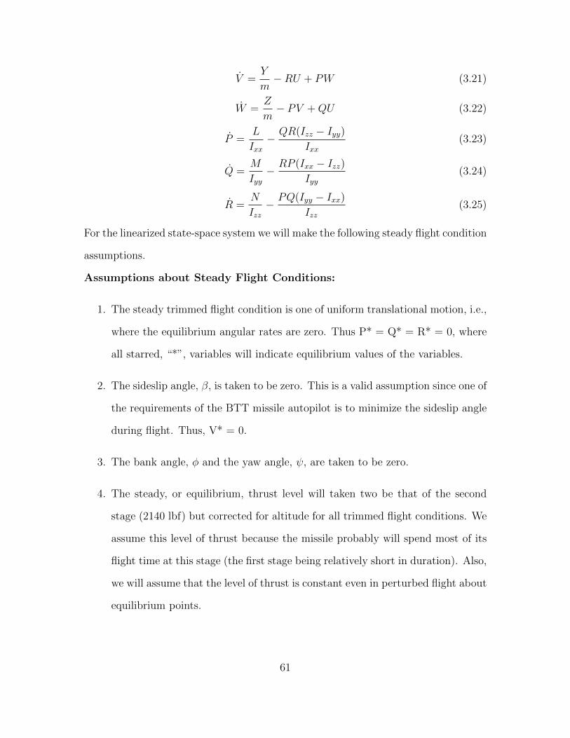
V =Y
m−RU + PW (3.21)
W =Z
m− PV +QU (3.22)
P =L
Ixx− QR(Izz − Iyy)
Ixx(3.23)
Q =M
Iyy− RP (Ixx − Izz)
Iyy(3.24)
R =N
Izz− PQ(Iyy − Ixx)
Izz(3.25)
For the linearized state-space system we will make the following steady flight condition
assumptions.
Assumptions about Steady Flight Conditions:
1. The steady trimmed flight condition is one of uniform translational motion, i.e.,
where the equilibrium angular rates are zero. Thus P* = Q* = R* = 0, where
all starred, “*”, variables will indicate equilibrium values of the variables.
2. The sideslip angle, β, is taken to be zero. This is a valid assumption since one of
the requirements of the BTT missile autopilot is to minimize the sideslip angle
during flight. Thus, V* = 0.
3. The bank angle, φ and the yaw angle, ψ, are taken to be zero.
4. The steady, or equilibrium, thrust level will taken two be that of the second
stage (2140 lbf) but corrected for altitude for all trimmed flight conditions. We
assume this level of thrust because the missile probably will spend most of its
flight time at this stage (the first stage being relatively short in duration). Also,
we will assume that the level of thrust is constant even in perturbed flight about
equilibrium points.
61

5. The missile’s mass properties change with flight time, as discussed in Chapter
2; However, for simplicity we assume that they are constant about trimmed
flight conditions. The eigenvalues of the linear EOM will be evaluated about
the same trim conditions but at different flight times to gage the affects of the
flight-time dependent mass properties.
∆U =∆X
m∗−W ∗∆Q (3.26)
∆V =∆Y
m∗− U∗∆R +W ∗∆P (3.27)
∆W =∆Z
m∗− U∗∆Q (3.28)
∆P =∆L
I∗xx(3.29)
∆Q =∆M
I∗yy(3.30)
∆R =∆N
I∗zz(3.31)
Under the above steady flight condition assumptions, we can write the perturbation
equations for the nonlinear Equations 3.20 - 3.25: where all starred, “*”, variables
indicate equilibrium values and where force and moment perturbations are
∆X = ∆Xaero + ∆FXg + ∆TX
∆Y = ∆Yaero + ∆FYg
∆Z = ∆Zaero + ∆FZg
∆L = ∆Laero
∆M = ∆Maero + ∆Mg
∆N = ∆Naero + ∆Ng
(3.32)
However, under assumptions (2) and (iv), we have
62

∆TX = ∆Mg = ∆Ng = 0
The gravitational force perturbations are as follows:
∆FXg = −mg cos(θ∗)∆θ
∆FYg = mg cos(θ∗) cos(φ∗)∆φ−mg sin(θ∗) sin(φ∗)∆θ
∆FZg = −mg cos(θ∗) sin(φ∗)∆φ−mg sin(θ∗) cos(φ∗)∆θ
(3.33)
However, under flight condition assumption 3, i.e., φ∗ = 0, Equations 3.33 reduce to
∆FXg = −mg cos(θ∗)∆θ
∆FYg = mg cos(θ∗)∆φ
∆FZg = −mg sin(θ∗)∆θ
(3.34)
The form of the aerodynamic forces and moments in Equations 3.16 (i.e., the stability
derivative representation) gives us valuable information on their dependencies on the
state and control variables. For example, lets consider the Taylor series expansion of
the aerodynamic pitch moment, M:
∆M = Qdp∗SrefLref∆CM + ρ∗Vb
∗SrefLrefCM∗∆Vb
NOTE: CM∗ and the other trimmed aerodynamic moment coefficients are not nec-
essarily zero because the missile’s c.g. is not located at body fixed-frame (except at t
= 0 because the body axis is fixed to the time-zero location of the c.g. and where we
assume that all of the aerodynamic data is referenced from). However, under ideal-
ization (2), we will assume XCG is zero, and thus, all trimmed moment aerodynamic
coefficients are zero. This will be more apparent in Section 3.3, where we discuss the
trim, or equilibrium, conditions of the missile.
From Equations 3.16, we can immediately see that
63
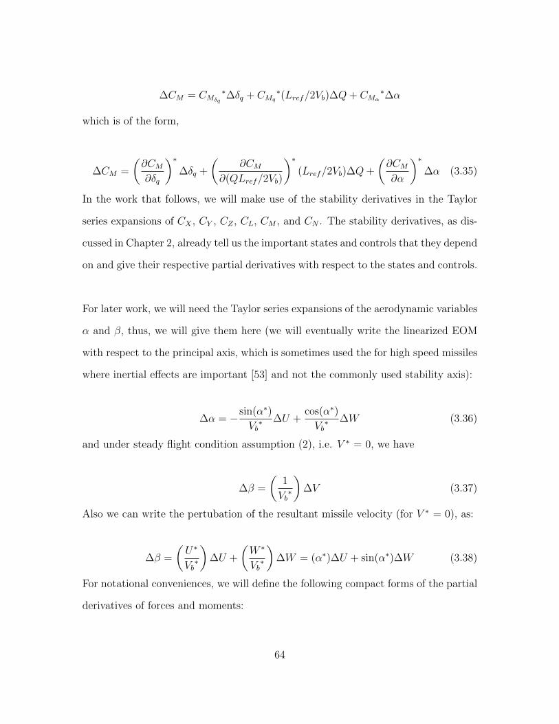
∆CM = CMδq
∗∆δq + CMq
∗(Lref/2Vb)∆Q+ CMα
∗∆α
which is of the form,
∆CM =
(∂CM∂δq
)∗∆δq +
(∂CM
∂(QLref/2Vb)
)∗(Lref/2Vb)∆Q+
(∂CM∂α
)∗∆α (3.35)
In the work that follows, we will make use of the stability derivatives in the Taylor
series expansions of CX , CY , CZ , CL, CM , and CN . The stability derivatives, as dis-
cussed in Chapter 2, already tell us the important states and controls that they depend
on and give their respective partial derivatives with respect to the states and controls.
For later work, we will need the Taylor series expansions of the aerodynamic variables
α and β, thus, we will give them here (we will eventually write the linearized EOM
with respect to the principal axis, which is sometimes used the for high speed missiles
where inertial effects are important [53] and not the commonly used stability axis):
∆α = −sin(α∗)
Vb∗ ∆U +
cos(α∗)
Vb∗ ∆W (3.36)
and under steady flight condition assumption (2), i.e. V ∗ = 0, we have
∆β =
(1
Vb∗
)∆V (3.37)
Also we can write the pertubation of the resultant missile velocity (for V ∗ = 0), as:
∆β =
(U∗
Vb∗
)∆U +
(W ∗
Vb∗
)∆W = (α∗)∆U + sin(α∗)∆W (3.38)
For notational conveniences, we will define the following compact forms of the partial
derivatives of forces and moments:
64

Partial Derivatives of Forces:
Xu∗ =
1
m∗
(∂X
∂U
)∗Zw∗ =
1
m∗
(∂Z
∂W
)∗and etc...
Partial Derivatives of Moments:
Mw∗ =
1
Iyy∗
(∂M
∂W
)∗Nv∗ =
1
Izz∗
(∂N
∂V
)∗and etc...
By inspection of the right hand sides of Equations 3.16, i.e., the stability derivative
representation of the aerodynamic forces and moments, and making use of Equations
3.36-3.38, we can write the following perturbation equations:
X-component of Translational Acceleration:
∆U = Xu∗∆U +Xw
∗∆W +Xq∗∆Q− (g∗ cos θ∗)∆θ (3.39)
where
Xu∗ =
(Qdp
∗Srefm∗Vb
∗
)2CX
∗ cosα∗
Xw∗ =
(Qdp
∗Srefm∗Vb
∗
)2CX
∗ sinα∗
65

Xq∗ = −W ∗
Y-component of Translational Acceleration:
∆V = Yu∗∆U+Yv
∗∆V +Yw∗∆W +Yp
∗∆P +Yr∗∆R+Yδr
∗∆δr+(g∗cosθ∗)∆φ (3.40)
where
Yu∗ =
(Qdp
∗Srefm∗Vb
∗
)2CY
∗ cosα∗
Yv∗ =
(Qdp
∗Srefm∗Vb
∗
)CNβ
∗
Yw∗ =
(Qdp
∗Srefm∗Vb
∗
)2CY
∗ sinα∗
Yp∗ = W ∗
Yr∗ = −U∗
Yδr∗ =
(Qdp
∗Srefm∗Vb
∗
)CYδr
∗
Z-component of Translational Acceleration:
∆W = Zu∗∆U + Zw
∗∆W + Zq∗∆Q+ Zδq
∗∆δq − (g∗ sin θ∗)∆θ (3.41)
where
Zu∗ = Qdp
∗Sref
(2CZ
∗ cosα∗ − CNα∗ sinα∗
m∗Vb∗
)Zw∗ = Qdp
∗Sref
(2CZ
∗ sinα∗ + CNα∗ cosα∗
m∗Vb∗
)Zq∗ = U∗
Zδq∗ =
(Qdp
∗Srefm∗
)CNδq
∗
66
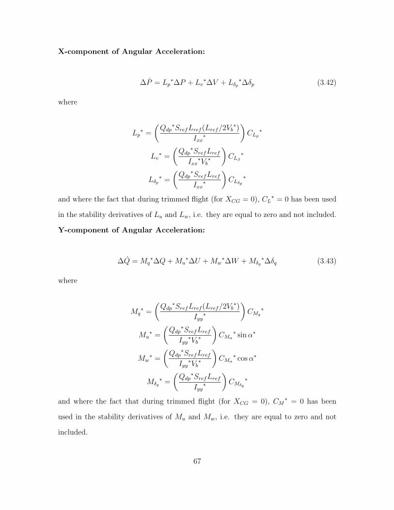
X-component of Angular Acceleration:
∆P = Lp∗∆P + Lv
∗∆V + Lδp∗∆δp (3.42)
where
Lp∗ =
(Qdp
∗SrefLref (Lref/2Vb∗)
Ixx∗
)CLp
∗
Lv∗ =
(Qdp
∗SrefLrefIxx∗Vb∗
)CLβ
∗
Lδp∗ =
(Qdp
∗SrefLrefIxx∗
)CLδp
∗
and where the fact that during trimmed flight (for XCG = 0), CL∗ = 0 has been used
in the stability derivatives of Lu and Lw, i.e. they are equal to zero and not included.
Y-component of Angular Acceleration:
∆Q = Mq∗∆Q+Mu
∗∆U +Mw∗∆W +Mδq
∗∆δq (3.43)
where
Mq∗ =
(Qdp
∗SrefLref (Lref/2Vb∗)
Iyy∗
)CMq
∗
Mu∗ =
(Qdp
∗SrefLrefIyy∗Vb∗
)CMα
∗ sinα∗
Mw∗ =
(Qdp
∗SrefLrefIyy∗Vb∗
)CMα
∗ cosα∗
Mδq∗ =
(Qdp
∗SrefLrefIyy∗
)CMδq
∗
and where the fact that during trimmed flight (for XCG = 0), CM∗ = 0 has been
used in the stability derivatives of Mu and Mw, i.e. they are equal to zero and not
included.
67

Z-component of Angular Acceleration:
∆R = Nr∗∆R +Nv
∗∆V +Nδr∗∆δr (3.44)
where
Nr∗ =
(Qdp
∗SrefLref (Lref/2Vb∗)
Izz∗
)CNr
∗
Nv∗ =
(Qdp
∗SrefLrefIzz∗Vb∗
)CNβ
∗
Nδr∗ =
(Qdp
∗SrefLrefIzz∗
)CNδr
∗
and where the fact that during trimmed flight (for XCG = 0), CN∗ = 0 has been used
in the stability derivatives of Nu and Nw, i.e. they are equal to zero and not included.
Equations 3.39 - 3.44 can be put into the following compact state equation form:
∆U
∆V
∆W
∆P
∆Q
∆R
∆φ
∆θ
=
Xu∗ 0 Xw∗ 0 Xq∗ 0 0 −g cos θ∗
Yu∗ Yv∗ Yw∗ Yp∗ 0 Yr∗ g cos θ∗ 0
Zu∗ 0 Zw∗ 0 Zq∗ 0 0 −g sin θ∗
0 Lv∗ 0 Lp∗ 0 0 0 0
Mu∗ 0 Mw
∗ 0 Mq∗ 0 0 0
0 Nv∗ 0 0 0 Nr∗ 0 0
0 0 0 1 0 0 0 0
0 0 0 0 1 0 0 0
∆U
∆V
∆W
∆P
∆Q
∆R
∆φ
∆θ
+
0 0 0
0 0 Yδr∗
0 Zδq∗ 0
Lδp∗ 0 0
0 Mδq∗ 0
0 0 Nδr∗
0 0 0
0 0 0
δp
δq
δr
(3.45)
where in the Equations 3.45, we have used for small perturbations that the Euler
angles (bank angle and attitude), only retaining 1st order terms, can be approximated
as:
∆φ = ∆P (3.46)
68

∆θ = ∆Q (3.47)
Finally Equations 3.45 yield the linear state-space equations of the BTT missile (under
the assumptions in the section).
3.3 Calculation of Equilibrium Points
From Section 3.2, (x∗, u∗) is an equilibrium point of Equation 3.1 for all t ≥ 0.
f(t, x∗, u∗) = 0 (3.48)
Thus, equations 3.9-3.14, for the assumptions of zero angular and translational
accelerations and the assumptions about ignoring the time rates of change of the
mass, mass moments of inertia, and c.g. location yield
X∗ = FXaero∗ + FXg
∗ + TX∗ = 0
Y ∗ = FYaero∗ + FYg
∗ = 0
Z∗ = FZaero∗ + FZg
∗ = 0
L∗ = Laero∗ = 0
M∗ = Maero∗ +Mg
∗ = 0
N∗ = Naero∗ +Ng
∗ = 0
(3.49)
For now, we will assume XCG is not zero only to see what effect our earlier
idealization that XCG = 0 has on our linear EOM. Substituting for the aerodynamic
and gravitational forces and moments into Equation 3.49 using Equations 3.16 and
3.17 and rearranging yields
69

and
X : QdpSrefCX = mg sin θ − Tx
Y : QdpSrefCY = −mg cos θ sinφ
Z : QdpSrefCZ = −mg cos θ cosφ
L : QdpSrefLrefCL = 0
M : QdpSrefLrefCM = XCGmg cos θ cosφ
N : QdpSrefLrefCN = −XCGmg cos θ sinφ
(3.50)
If we assume some level of thrust Tx, we can solve for the trimmed aerodynamic
coefficients CX , CY , CZ , CL, CM , and CN . The values of the aerodynamic coefficients
in trimmed flight are given as follows:
CX∗ =
mg sin θ∗ − Tx∗
Qdp∗Sref
CY∗ =−mg cos θ∗ sinφ∗
Qdp∗Sref
CZ∗ =−mg cos θ∗ cosφ∗
Qdp∗Sref
CL∗ = 0
CM∗ =
XCGmg cos θ∗ cosφ∗
Qdp∗SrefLref
CN∗ =−XCGmg cos θ∗ sinφ∗
Qdp∗SrefLref
(3.51)
From idealization (2), i.e., XCG = 0, CM∗ = CN
∗ = 0. In addition, CY∗ = 0
under the previous idealization that the missiles bank angle is zero (φ = 0). These
idealizations were accounted for in all linear equations presented in the previous
section. From the above Equations 3.51, we can see that when we assume that the
equilibrium value of the c.g. location is zero that the trimmed values of CM and
CN are zero. Also from equations 3.51, we can see even if XCG is non-zero but
relatively “small” that at “high” missile velocities and low missile altitudes (this
70

gives large Qdp) that the trimmed values of CM and CN are “small” and that the
idealization that XCG = 0 is valid. However, this might not be a valid idealization
for a “slow” moving aircraft, such as one approaching for landing, or for very “large”
c.g. displacements.
In Section 2.4, the BTT missile stability derivatives were presented and Table 2.3
summarized their dependence on other variables. Using Table 2.3 as reference, Equa-
tions 3.51 are rewritten to emphasize their dependence on the stability derivatives
(also XCG is assumed to be zero, as discussed previously):
The m-file “btt linr.m” uses the above equations, given a user specified trim angle
of attack, α∗, and altitude, to iterate for the corresponding Mach number and actuator
deflection δq.
CD(δq∗,M∗, α∗) + CDT (M∗) =
mg sin θ∗ − Tx∗
Qdp∗Sref
CYβ(M∗, α∗)β∗ + CYδr (M∗, β∗)δr
∗ =−mg cos θ∗ sinφ∗
Qdp∗Sref
CNα(M∗)α∗ + CNδq (M∗, α∗)δq
∗ =−mg cos θ∗ cosφ∗
Qdp∗Sref
CLδp (M∗, α∗)δp∗ + CLp(M
∗, α∗)(Lref/2Vb)P∗ + CLβ(M∗, α∗)β∗ = 0
CMδq(M∗, α∗)δq
∗ + CMq(M∗, α∗)(Lref/2Vb)Q
∗ + CMα(M∗, α∗)α∗ = 0
CNδr (M∗, β∗)δr
∗ + CNr(M∗, β∗)(Lref/2Vb)R
∗ + CNβ(M∗, α∗)β∗ = 0
(3.52)
Under Steady state flight assumptions (i) and (ii), equations 3.52 can be rewritten
as follows:
71

CD(δq∗,M∗, α∗) + CDT (M∗) =
mg sin θ∗ − Tx∗
Qdp∗Sref
CYδr (M∗, β∗)δr
∗ =−mg cos θ∗sinφ∗
Qdp∗Sref
= 0, (∵ φ = 0)
CNα(M∗)α∗ + CNδq (M∗, α∗)δq
∗ =−mg cos θ∗
Qdp∗Sref
δp∗ = 0
δq∗ =−CMα(M∗, α∗)
CMδq(M∗, α∗)
α∗, (Solved for δq)
δr∗ = 0
(3.53)
The m-file “btt linr.m” uses the above equations, given a user specified trim angle
of attack, α∗, and altitude, to iterate for the corresponding Mach number and actuator
deflection δq.
3.4 Scaled Linear BTT Missile State-Space System
In this section, the linear EOM derived in the previous section are dimension-
ally scaled. A dimensionally scaled state-space system is desirable for the following
reasons:
1. Modal analysis of the state-space system to determine the systems natural ten-
dencies is easier to interpret when all of the system equations have the same
units. This makes comparisons between translational and rotational modes of
the same (scaled) size.
2. Multivariable control theory such as the H∞ design method essentially “shape”
the systems transfer function matrix (TFM) singular value bode magnitude
plots based upon some user supplied weightings on performance and/or robust-
ness. It is well known that singular values are unit sensitive and thus it is
72

desirable that we have singular value loop shapes that have the same units such
that we are comparing “apples to apples” and not “apples to oranges”.
3. From a properly done dimensional analysis (i.e., a properly scaled system), a
simple observation of the systems terms is all that is necessary to determine the
relative importance of the dependent variables in the EOM. This is an invaluable
tool during model reduction.
Non-dimensional State Equations:
In our dimensional analysis we will define the following non-dimensional quantities:
u ≡ ∆U
Vb∗
v ≡ ∆V
Vb∗
w ≡ ∆W
Vb∗
p ≡ t∆P
q ≡ t∆Q
r ≡ t∆R
(3.54)
where
t ≡ mVb∗
Qdp∗Sref
, (sec) (3.55)
and where we define the non-dimensional aerodynamic time, τ , as
τ ≡ t
t(3.56)
From Equation 3.56, we can see that the differentiation operator now becomes
d()
dt=
1
t
d()
dτ=Qdp
∗SrefmVb
∗d()
dτ(3.57)
dt = t dτ .
73

Substituting for ∆U,∆V,∆W,∆P,∆Q, and ∆R in equations 3.39 - 3.44 using
equations 3.54 and also substituting for the differentiation operator using equation
3.57 and then dividing through the resulting equations by Vb∗ yields the following
non-dimensional equations of motion:
˙u = xu∗u+ xw
∗w + xq∗q − g cos θ∗∆θ (3.58)
˙v = yu∗u+ yv
∗v + yw∗w + yp
∗p+ yr∗r + g cos θ∗∆φ (3.59)
˙w = zu∗u+ zw
∗w + zq∗q + zδq
∗∆δq − g sin θ∗∆θ (3.60)
˙p = lp∗p+ lv
∗v + lδp∗∆δp (3.61)
˙q = mu∗u+mw
∗w +mq∗q +mδq
∗∆δq (3.62)
˙r = nv∗v + nr
∗r + nδr∗∆δr (3.63)
where
g ≡ m∗g
Qdp∗Sref
(3.64)
The lower case stability derivatives are dimensionless are related to the previously
defined stability derivatives as follows:
xu∗ =
(m∗Vb
∗
Qdp∗Sref
)Xu∗ = 2CX
∗ cosα∗
xw∗ =
(m∗Vb
∗
Qdp∗Sref
)Xw∗ = 2CX
∗ sinα∗
xq∗ =
(1
Vb∗
)Xq∗ = −
(W ∗
Vb∗
)= sinα∗
yu∗ =
(m∗Vb
∗
Qdp∗Sref
)Yu∗ = 2CY
∗ cosα∗
yv∗ =
(m∗Vb
∗
Qdp∗Sref
)Yv∗ = CNβ
∗
74

yw∗ =
(m∗Vb
∗
Qdp∗Sref
)Yw∗ = 2CY
∗ sinα∗
yp∗ =
(1
Vb∗
)Yp∗ =
(W ∗
Vb∗
)= sinα∗
yr∗ =
(1
Vb∗
)Yr∗ = −
(U∗
Vb∗
)= − cosα∗
yδr∗ =
(m∗
Qdp∗Sref
)Yδr∗ = CYδr
∗
zu∗ =
(m∗Vb
∗
Qdp∗Sref
)Zu∗ = 2CZ
∗ cosα∗ − CNα∗ sinα∗
zw∗ =
(m∗Vb
∗
Qdp∗Sref
)Zw∗ = 2CZ
∗ sinα∗ + CNα∗ cosα∗
zq∗ =
(1
Vb∗
)Zq∗ =
(U∗
Vb∗
)= cosα∗
zδq∗ =
(m∗
Qdp∗Sref
)Zδq∗ = CNδq
∗
lp∗ =
(m∗Vb
∗
Qdp∗Sref
)Lp∗ =
(12m∗Lref
2
Ixx∗
)CLp
∗
lv∗ =
(m∗Vb
∗
Qdp∗Sref
)2
Vb∗Lv
∗ =
(2m∗2Lrefρ∗SrefIxx
∗
)CLβ
∗
lδp∗ =
(m∗Vb
∗
Qdp∗Sref
)2
Lδp∗ =
(2m∗2Lrefρ∗SrefIxx
∗
)CLδp
∗
mu∗ =
(m∗Vb
∗
Qdp∗Sref
)2
Vb∗Mu
∗ = −(
2m∗2Lrefρ∗SrefIyy
∗
)CMα
∗ sinα∗
mw∗ =
(m∗Vb
∗
Qdp∗Sref
)2
Vb∗Mw
∗ =
(2m∗2Lrefρ∗SrefIyy
∗
)CMα
∗ cosα∗
mq∗ =
(m∗Vb
∗
Qdp∗Sref
)Mq∗ =
(12m∗Lref
2
Iyy∗
)CMq
∗
mδq∗ =
(m∗Vb
∗
Qdp∗Sref
)2
Mδq∗ =
(2m∗2Lrefρ∗SrefIyy
∗
)CMδq
∗
nv∗ =
(m∗Vb
∗
Qdp∗Sref
)2
Vb∗Nv
∗ =
(2m∗2Lrefρ∗SrefIzz
∗
)CNβ
∗
75

nr∗ =
(m∗Vb
∗
Qdp∗Sref
)Nr∗ =
(12m∗Lref
2
Izz∗
)CNr
∗
nδr∗ =
(m∗Vb
∗
Qdp∗Sref
)2
Nδr∗ =
(2m∗2Lrefρ∗SrefIzz
∗
)CNδr
∗
Using Equations 3.55 - 3.64 and the above defined non-dimensional stability
derivatives, we can write the state equations in the following compact form:
˙u
˙v
˙w
˙p
˙q
˙r
∆φ
∆θ
=
xu∗ 0 xw∗ 0 xq∗ 0 0 −g cos θ∗
yu∗ yv∗ yw∗ yp∗ 0 yr∗ g cos θ∗ 0
zu∗ 0 zw∗ 0 zq∗ 0 0 −g sin θ∗
0 lv∗ 0 lp
∗ 0 0 0 0
mu∗ 0 mw∗ 0 mq∗ 0 0 0
0 nv∗ 0 0 0 nr∗ 0 0
0 0 0 1 0 0 0 0
0 0 0 0 1 0 0 0
u
v
w
p
q
r
∆φ
∆θ
+
0 0 0
0 0 yδr∗
0 zδq∗ 0
lδp∗ 0 0
0 mδq∗ 0
0 0 nδr∗
0 0 0
0 0 0
δp
δq
δr
(3.65)
where in Equation 3.65, we have made use of the fact that
1
t
d(∆φ)
dτ=
1
tp
or simply
d(∆φ)
dτ= p
and similarly,
d(∆θ)
dτ= q
Note that v is the sideslip angle, ∆β, under the assumption the equilibrium value
of V is zero. However, w is only approximately equal to ∆α for “small” equilibrium
or reference values of α since we are using the principal body axis and not the sta-
bility axis for our linearized state-space system. Now that we have missile dynamics
76
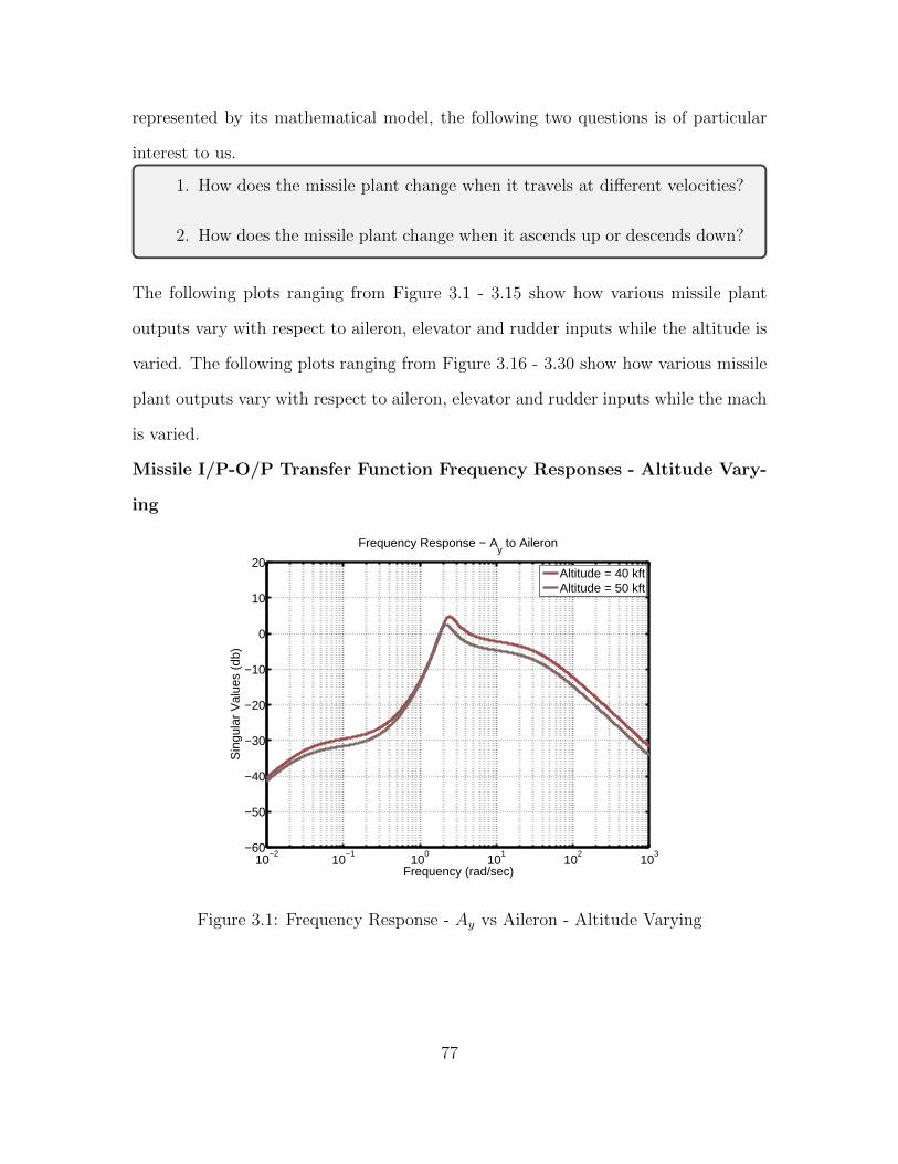
represented by its mathematical model, the following two questions is of particular
interest to us.
1. How does the missile plant change when it travels at different velocities?
2. How does the missile plant change when it ascends up or descends down?
The following plots ranging from Figure 3.1 - 3.15 show how various missile plant
outputs vary with respect to aileron, elevator and rudder inputs while the altitude is
varied. The following plots ranging from Figure 3.16 - 3.30 show how various missile
plant outputs vary with respect to aileron, elevator and rudder inputs while the mach
is varied.
Missile I/P-O/P Transfer Function Frequency Responses - Altitude Vary-
ing
10−2
10−1
100
101
102
103−60
−50
−40
−30
−20
−10
0
10
20
Frequency Response − Ay to Aileron
Frequency (rad/sec)
Sin
gula
r V
alue
s (d
b)
Altitude = 40 kftAltitude = 50 kft
Figure 3.1: Frequency Response - Ay vs Aileron - Altitude Varying
77

10−2
10−1
100
101
102
103−30
−20
−10
0
10
20
30
Frequency Response − Ay to Rudder
Frequency (rad/sec)
Sin
gula
r V
alue
s (d
b)
Altitude = 40 kftAltitude = 50 kft
Figure 3.2: Frequency Response - Ay vs Rudder - Altitude Varying
10−1
100
101
102
−40
−35
−30
−25
−20
−15
−10
−5
0
5
Frequency Response − Az to Elevator
Frequency (rad/sec)
Sin
gula
r V
alue
s (d
b)
Altitude = 40 kftAltitude = 50 kft
Figure 3.3: Frequency Response - Az vs Elevator - Altitude Varying
78

10−1
100
101
102
−60
−50
−40
−30
−20
−10
0
10
20
30
40
Frequency Response − φ to Aileron
Frequency (rad/sec)
Sin
gula
r V
alue
s (d
b)
Altitude = 40 kftAltitude = 50 kft
Figure 3.4: Frequency Response - φ vs Aileron - Altitude Varying
10−1
100
101
102
103
−140
−120
−100
−80
−60
−40
−20
0
20
40
Frequency Response − φ to Rudder
Frequency (rad/sec)
Sin
gula
r V
alue
s (d
b)
Altitude = 40 kftAltitude = 50 kft
Figure 3.5: Frequency Response - φ vs Rudder - Altitude Varying
79

10−2
10−1
100
101
−45
−40
−35
−30
−25
−20
−15
−10
−5
0
Frequency Response − θ to Elevator
Frequency (rad/sec)
Sin
gula
r V
alue
s (d
b)
Altitude = 40 kftAltitude = 50 kft
Figure 3.6: Frequency Response - θ vs Elevator - Altitude Varying
10−2
10−1
100
101
102
103−80
−70
−60
−50
−40
−30
−20
−10
0
10Frequency Response − β to Aileron
Frequency (rad/sec)
Sin
gula
r V
alue
s (d
b)
Altitude = 40 kftAltitude = 50 kft
Figure 3.7: Frequency Response - β vs Aileron - Altitude Varying
80

100
101
102
103
−100
−80
−60
−40
−20
0
Frequency Response − β to Rudder
Frequency (rad/sec)
Sin
gula
r V
alue
s (d
b)
Altitude = 40 kftAltitude = 50 kft
Figure 3.8: Frequency Response - β vs Rudder - Altitude Varying
10−1
100
101
−50
−40
−30
−20
−10
0
Frequency Response − α to Elevator
Frequency (rad/sec)
Sin
gula
r V
alue
s (d
b)
Altitude = 40 kftAltitude = 50 kft
Figure 3.9: Frequency Response - α vs Elevator - Altitude Varying
81
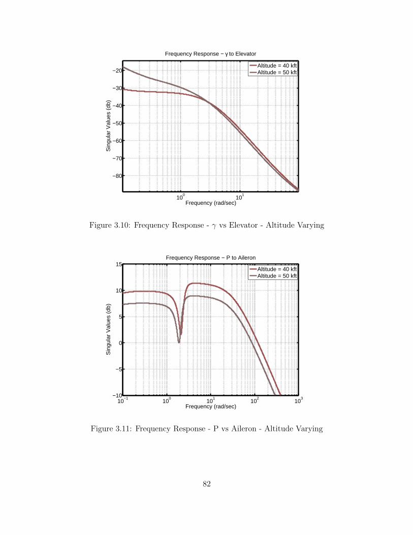
100
101
−80
−70
−60
−50
−40
−30
−20
Frequency Response − γ to Elevator
Frequency (rad/sec)
Sin
gula
r V
alue
s (d
b)
Altitude = 40 kftAltitude = 50 kft
Figure 3.10: Frequency Response - γ vs Elevator - Altitude Varying
10−1
100
101
102
103−10
−5
0
5
10
15Frequency Response − P to Aileron
Frequency (rad/sec)
Sin
gula
r V
alue
s (d
b)
Altitude = 40 kftAltitude = 50 kft
Figure 3.11: Frequency Response - P vs Aileron - Altitude Varying
82

10−2
10−1
100
101
102
103−100
−50
0
50Frequency Response − P to Rudder
Frequency (rad/sec)
Sin
gula
r V
alue
s (d
b)
Altitude = 40 kftAltitude = 50 kft
Figure 3.12: Frequency Response - P vs Rudder - Altitude Varying
10−2
10−1
100
101
102
103−40
−30
−20
−10
0
10
20Frequency Response − Q to Elevator
Frequency (rad/sec)
Sin
gula
r V
alue
s (d
b)
Altitude = 40 kftAltitude = 50 kft
Figure 3.13: Frequency Response - Q vs Elevator - Altitude Varying
83

10−2
10−1
100
101
102
103−120
−100
−80
−60
−40
−20
0
20
Frequency Response − R to Aileron
Frequency (rad/sec)
Sin
gula
r V
alue
s (d
b)
Altitude = 40 kftAltitude = 50 kft
Figure 3.14: Frequency Response - R vs Aileron - Altitude Varying
10−2
10−1
100
101
102
103−30
−20
−10
0
10
20
30Frequency Response − R to Rudder
Frequency (rad/sec)
Sin
gula
r V
alue
s (d
b)
Altitude = 40 kftAltitude = 50 kft
Figure 3.15: Frequency Response - R vs Rudder - Altitude Varying
Missile I/P-O/P Transfer Function Frequency Responses - Mach Varying
84

10−2
10−1
100
101
102
103−60
−50
−40
−30
−20
−10
0
10
20
Frequency Response − Ay to Aileron
Frequency (rad/sec)
Sin
gula
r V
alue
s (d
b)
Mach = 1.068Mach = 1.5114
Figure 3.16: Frequency Response - Ay vs Aileron - Mach Varying
10−2
10−1
100
101
102
103−30
−20
−10
0
10
20
30
Frequency Response − Ay to Rudder
Frequency (rad/sec)
Sin
gula
r V
alue
s (d
b)
Mach = 1.068Mach = 1.5114
Figure 3.17: Frequency Response - Ay vs Rudder - Mach Varying
85

10−2
10−1
100
101
102
103−50
−40
−30
−20
−10
0
10
Frequency Response − Az to Elevator
Frequency (rad/sec)
Sin
gula
r V
alue
s (d
b)
Mach = 1.068Mach = 1.5114
Figure 3.18: Frequency Response - Az vs Elevator - Mach Varying
10−2
10−1
100
101
102
103
−60
−40
−20
0
20
40
60
Frequency Response − φ to Aileron
Frequency (rad/sec)
Sin
gula
r V
alue
s (d
b)
Mach = 1.068Mach = 1.5114
Figure 3.19: Frequency Response - φ vs Aileron - Mach Varying
86

10−2
10−1
100
101
102
103−150
−100
−50
0
50
Frequency Response − φ to Rudder
Frequency (rad/sec)
Sin
gula
r V
alue
s (d
b)
Mach = 1.068Mach = 1.5114
Figure 3.20: Frequency Response - φ vs Rudder - Mach Varying
10−3
10−2
10−1
100
101
102−50
−40
−30
−20
−10
0
10
20
Frequency Response − θ to Elevator
Frequency (rad/sec)
Sin
gula
r V
alue
s (d
b)
Mach = 1.068Mach = 1.5114
Figure 3.21: Frequency Response - θ vs Elevator - Mach Varying
87

10−2
10−1
100
101
102
103−80
−70
−60
−50
−40
−30
−20
−10
0
10Frequency Response − β to Aileron
Frequency (rad/sec)
Sin
gula
r V
alue
s (d
b)
Mach = 1.068Mach = 1.5114
Figure 3.22: Frequency Response - β vs Aileron - Mach Varying
10−2
10−1
100
101
102
103−100
−80
−60
−40
−20
0
20
Frequency Response − β to Rudder
Frequency (rad/sec)
Sin
gula
r V
alue
s (d
b)
Mach = 1.068Mach = 1.5114
Figure 3.23: Frequency Response - β vs Rudder - Mach Varying
88
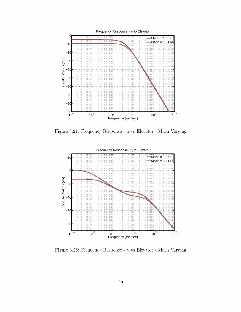
10−2
10−1
100
101
102
103−90
−80
−70
−60
−50
−40
−30
−20
−10
0Frequency Response − α to Elevator
Frequency (rad/sec)
Sin
gula
r V
alue
s (d
b)
Mach = 1.068Mach = 1.5114
Figure 3.24: Frequency Response - α vs Elevator - Mach Varying
10−3
10−2
10−1
100
101
102
−80
−60
−40
−20
0
20
Frequency Response − γ to Elevator
Frequency (rad/sec)
Sin
gula
r V
alue
s (d
b)
Mach = 1.068Mach = 1.5114
Figure 3.25: Frequency Response - γ vs Elevator - Mach Varying
89

10−2
10−1
100
101
102
103−10
−5
0
5
10
15
20
25
30Frequency Response − P to Aileron
Frequency (rad/sec)
Sin
gula
r V
alue
s (d
b)
Mach = 1.068Mach = 1.5114
Figure 3.26: Frequency Response - P vs Aileron - Mach Varying
10−2
10−1
100
101
102
103−100
−50
0
50Frequency Response − P to Rudder
Frequency (rad/sec)
Sin
gula
r V
alue
s (d
b)
Mach = 1.068Mach = 1.5114
Figure 3.27: Frequency Response - P vs Rudder - Mach Varying
90

10−2
10−1
100
101
102
103−40
−30
−20
−10
0
10
20Frequency Response − Q to Elevator
Frequency (rad/sec)
Sin
gula
r V
alue
s (d
b)
Mach = 1.068Mach = 1.5114
Figure 3.28: Frequency Response - Q vs Elevator - Mach Varying
10−2
10−1
100
101
102
103−120
−100
−80
−60
−40
−20
0
20Frequency Response − R to Aileron
Frequency (rad/sec)
Sin
gula
r V
alue
s (d
b)
Mach = 1.068Mach = 1.5114
Figure 3.29: Frequency Response - R vs Aileron - Mach Varying
91

10−2
10−1
100
101
102
103−30
−20
−10
0
10
20
30Frequency Response − R to Rudder
Frequency (rad/sec)
Sin
gula
r V
alue
s (d
b)
Mach = 1.068Mach = 1.5114
Figure 3.30: Frequency Response - R vs Rudder - Mach Varying
3.5 Discussion of BTT Missile Natural Modes (Eigenvalues)
Using the non-dimensional linear system of equations, equation 3.65, and the iter-
ative trim procedure in MATLAB m-file “missile plant analysis.m”, the characteristic
modes of the BTT missile were investigated for the steady flight condition discussed
in Section 3.2. The plant dynamics, or “A” matrix, of equation 3.65 was used in its
presented form to find the characteristic modes of the missile. The condition number
of the A-matrix in equation 3.65 was very large (>1 × 10⁶) due to the integration
of p and q for φ and θ, respectively. After observing the relative sizes of the non-
dimensional terms and the very weak longitudinal and lateral dynamic coupling, the
following reduced systems are used for determining the characteristic modes:
92
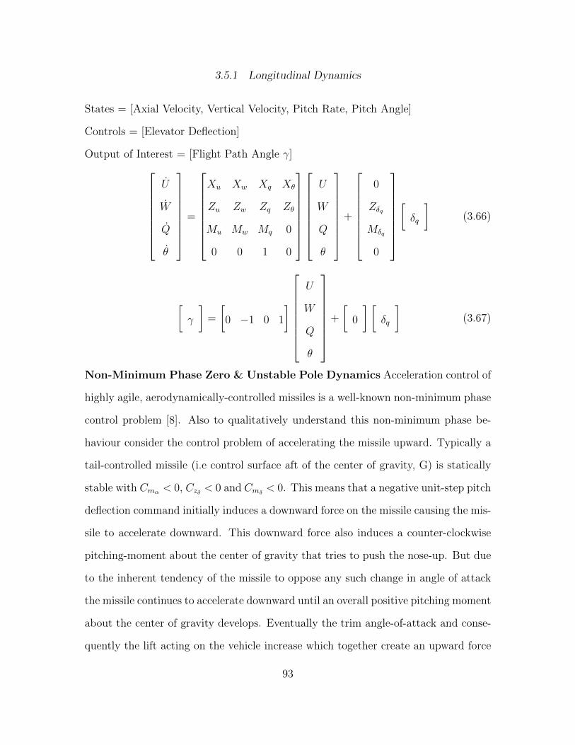
3.5.1 Longitudinal Dynamics
States = [Axial Velocity, Vertical Velocity, Pitch Rate, Pitch Angle]
Controls = [Elevator Deflection]
Output of Interest = [Flight Path Angle γ]
U
W
Q
θ
=
Xu Xw Xq Xθ
Zu Zw Zq Zθ
Mu Mw Mq 0
0 0 1 0
U
W
Q
θ
+
0
Zδq
Mδq
0
[δq
](3.66)
[γ
]=
[0 −1 0 1
]
U
W
Q
θ
+
[0
] [δq
](3.67)
Non-Minimum Phase Zero & Unstable Pole Dynamics Acceleration control of
highly agile, aerodynamically-controlled missiles is a well-known non-minimum phase
control problem [8]. Also to qualitatively understand this non-minimum phase be-
haviour consider the control problem of accelerating the missile upward. Typically a
tail-controlled missile (i.e control surface aft of the center of gravity, G) is statically
stable with Cmα < 0, Czδ < 0 and Cmδ < 0. This means that a negative unit-step pitch
deflection command initially induces a downward force on the missile causing the mis-
sile to accelerate downward. This downward force also induces a counter-clockwise
pitching-moment about the center of gravity that tries to push the nose-up. But due
to the inherent tendency of the missile to oppose any such change in angle of attack
the missile continues to accelerate downward until an overall positive pitching moment
about the center of gravity develops. Eventually the trim angle-of-attack and conse-
quently the lift acting on the vehicle increase which together create an upward force
93

about the fuselage; and thus the missile accelerates upward as desired. The above
described non-minimum phase behaviour is a characteristic of several important tail
controlled aerospace flight control problems such as control of Vertical Take-off and
Landing (VTOL) aircraft, and Conventional Take-offand Landing (CTOL) aircraft.
Pitch-up instability phenomenon occurs when center of pressure moves forward due
to tip stall due to high angle of attack. Both the RHP Pole-Zero dynamics was cap-
tured here in linearization routine and their behaviour with different flight conditions
are explained below. The decoupled longitunal system exhibits nonminimum phase
behaviour with flight path angle dynamics. So naturally the below question arises in
our mind.
When does a Nonminimum phase system arise? What is the cause?
Subtracting two systems where one has slow & weak dynamics and other has
fast & strong dynamics will result in a nonminimum phase system.
Illustrative Example. Consider the following systems
Slow/Weak Dynamics - Fast/Strong Dynamics =3
s+ 1− 4
s+ 2
=3(s+ 2)− 4(s+ 1)
(s+ 1)(s+ 2)
=2− s
(s+ 1)(s+ 2)
The nonminimum phase flight path angle with respect to the elevator deflection dy-
namics can be explained below
λ(s)
δq(s)= Slow/Weak Dynamics - Fast/Strong Dynamics
=α(s)
δq(s)− θ(s)
δq(s)
94

This holds true even if we try with a perfectly decoupled longitudinal system as
both pitch and angle of attack parameters are longitudinal components. Similarly,
the control problem of acceleration in upward direction with respect to the elevator
deflection can be explained as follows
az = w − qu+ pv − cross coupling components
= Slow/Weak Dynamics - Fast/Strong Dynamics
So, if we neglect the inertial cross coulping terms during linearization, we won’t be
able to capture the nonminimum phase behaviour. That is why, here in this research
we get only minimum phase system here and this assumption is made to make the
control design easy, when the nonlinear dynamic inversion technique is applied to
get a nonlinear controller. This holds true even if we try with a perfectly decoupled
system as cross coupling terms won’t be present even there.
Thus, in general if two systems are combined such as g1s+p1− g2
s+p2, the process will
result in non-minimum phase behaviour if and only if
g1
p1
− g2
p2
> 0 and g1 − g2 < 0.
Effect of Coupling on Zero-dynamics. When you have a tightly coupled system,
the transmission zeros of the system are not the same as zeros in the plant input-
output transfer functions. But when systems are decoupled (like in our case), then
the transmission zeros of the system are the same as zeros in the plant input-output
transfer functions.
Missile experiences higher dynamic pressure, “Qdp” at lower altitudes, as a result of
which the pitch up instability and nonminimum phase behaviour is very strong at
those altitudes. And the magnitude of RHP pole and RHP zero decrease as altitude
95

increases. The above said behaviour is captured well in Figures 3.31 & 3.35. While
the effect of angle of attack on RHP pole-zero is opposite to that of altitude effects. As
angle of attack increases, both the magnitude of RHP pole and RHP zero increased.
This behaviour is captured well in Figures 3.33 & 3.37 respectively.
0 10 20 30 40 50 6010
20
30
40
50
60
70
80
90
100
110Longitudinal Plant RHP Zero Dynamics − Altitude Variation
Altitude (kft)
RH
P Z
ero
Loca
tion
α = 6 degα = 7 degα = 8 degα = 9 deg
Figure 3.31: Longitunal Plant RHP Zero Dynamics - Altitude Varying
96
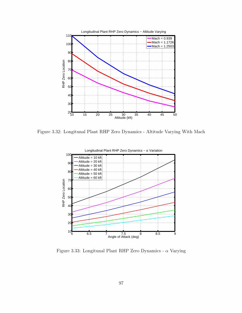
10 15 20 25 30 35 40 45 5020
30
40
50
60
70
80
90
100
110Longitudinal Plant RHP Zero Dynamics − Altitude Varying
Altitude (kft)
RH
P Z
ero
Loca
tion
Mach = 0.939Mach = 1.1726Mach = 1.2503
Figure 3.32: Longitunal Plant RHP Zero Dynamics - Altitude Varying With Mach
6 6.5 7 7.5 8 8.5 910
20
30
40
50
60
70
80
90
100Longitudinal Plant RHP Zero Dynamics − α Variation
Angle of Attack (deg)
RH
P Z
ero
Loca
tion
Altitude = 10 kftAltitude = 20 kftAltitude = 30 kftAltitude = 40 kftAltitude = 50 kftAltitude = 60 kft
Figure 3.33: Longitunal Plant RHP Zero Dynamics - α Varying
97

0.9 1 1.1 1.2 1.3 1.4 1.5 1.6 1.7 1.855
60
65
70
75
80
85
90
95
100Longitudinal Plant RHP Zero Dynamics − Mach Varying
Mach
RH
P Z
ero
Loca
tion
Altitude = 30 kftAltitude = 40 kftAltitude = 50 kft
Figure 3.34: Longitunal Plant RHP Zero Dynamics - Mach Varying
0 10 20 30 40 50 600
0.5
1
1.5
2
2.5
3
3.5
4
4.5Longitudinal Plant RHP Pole Dynamics − Altitude Variation
Altitude (kft)
RH
P P
ole
Loca
tion
α = 6 degα = 7 degα = 8 degα = 9 deg
Figure 3.35: Longitunal Plant RHP Pole Dynamics - Altitude Varying
98

10 15 20 25 30 35 40 45 503.5
4
4.5
5
5.5
6
6.5
7Longitudinal Plant RHP Pole Dynamics − Altitude Varying
Altitude (kft)
RH
P P
ole
Loca
tion
Mach = 1.5114Mach = 1.7731Mach = 2.0420
Figure 3.36: Longitunal Plant RHP Pole Dynamics - Altitude Varying With Mach
6 6.5 7 7.5 8 8.5 90
0.5
1
1.5
2
2.5
3
3.5
4
4.5Longitudinal Plant RHP Pole Dynamics − α Variation
Angle of Attack (deg)
RH
P P
ole
Loca
tion
Altitude = 10 kftAltitude = 20 kftAltitude = 30 kftAltitude = 40 kftAltitude = 50 kftAltitude = 60 kft
Figure 3.37: Longitunal Plant RHP Pole Dynamics - α Varying
99

0.9 1 1.1 1.2 1.3 1.42.5
3
3.5
4
4.5
5
5.5
6
6.5
7Longitudinal Plant RHP Pole Dynamics − Mach Varying
Mach
RH
P P
ole
Loca
tion
Altitude = 10 kftAltitude = 20 kftAltitude = 30 kftAltitude = 40 kft
Figure 3.38: Longitunal Plant RHP Pole Dynamics - Mach Varying
3.5.2 Lateral Dynamics
States = [Lateral Velocity, Roll rate, Yaw Rate , Roll Angle]
Controls = [Aileron Deflection, Rudder Deflection]
Output of Interest = [Roll φ, Roll Rate P, Sideslip β, Yaw Rate R]
V
P
R
φ
=
Yv Yp Yr Yφ
Lv Lp Lr 0
Nv Np Nr 0
0 1 0 0
V
P
R
φ
+
Yδp Yδr
Lδp Lδr
Nδp Nδr
0 0
δp
δr
(3.68)
β
P
R
φ
=
1 0 0 0
0 1 0 0
0 0 1 0
0 0 0 1
V
P
R
φ
+
0 0
0 0
δp
δr
(3.69)
100

20 25 30 35 40 45 50 55 600
0.2
0.4
0.6
0.8
1
1.2
1.4Lateral Plant RHP Pole Dynamics − Altitude Variation
Altitude (kft)
RH
P P
ole
Loca
tion
α = 12 degα = 13 degα = 14 degα = 15 deg
Figure 3.39: Lateral Plant RHP Pole Dynamics - Altitude Varying
12 12.5 13 13.5 14 14.5 150
0.2
0.4
0.6
0.8
1
1.2
1.4Lateral Plant RHP Pole Dynamics − α Variation
Angle of Attack (deg)
RH
P P
ole
Loca
tion
Altitude = 20 kftAltitude = 30 kftAltitude = 40 kftAltitude = 50 kftAltitude = 60 kft
Figure 3.40: Lateral Plant RHP Pole Dynamics - α Varying
101
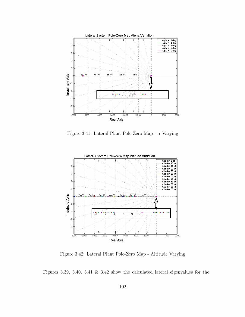
Figure 3.41: Lateral Plant Pole-Zero Map - α Varying
Figure 3.42: Lateral Plant Pole-Zero Map - Altitude Varying
Figures 3.39, 3.40, 3.41 & 3.42 show the calculated lateral eigenvalues for the
102

above non-dimensional A-matrices. The unstable pole denotes the “spiral divergence
mode”. This indicates a more sluggish response of the missile in the lateral direction
at higher altitudes. Similar to the longitudinal dynamics, the unstable poles of the
lateral dynamics move closer to the imaginary axis as altitude increases, while they
move deeper into the RHP plane when angle of attack is increased.
Tables 3.1 & 3.3 show the longitudinal and lateral eigenvalues for the above non-
dimensional A matrices when they are calculated for the missile flying at 10 kft and 40
kft respectively, for several different angles of attack, and initial time mass properties
(fully fuelled missile). Similarly Tables 3.2 & 3.4 show the longitudinal and lateral
eigenvalues for same angles of attack and altitude at 10 kft and 40 kft respectively
but for the “fuel-spent” mass properties of the missile (fuel depleted missile).
The system modes for the non-dimensional system are given by the following equation
(i.e., only if all the system eigenvalues are distinct):
~x(τ) =n∑i=1
(~pi ~x0)eλiτ ~qi =n∑i=1
(~pi ~x0)eλitt ~qi (3.70)
where
~pidef= Left eigenvector of A associated with λi
~qidef= Right eigenvector of A associated with λi
From equation (3.70) we can see that the aerodynamic time scaling factor given by
equation 3.71
tdef=
mVb∗
Qdp∗Sref
=2m
ρ∗Vb∗Sref
(3.71)
scales the response time of each mode. Since this is the case, we can see that the
missiles mass, altitude (ρ is dependent on altitude), velocity magnitude, and aerody-
namic reference area are very important in determining missile responsiveness. This
103

is evident from lateral eigenvalues from tables 3.1 & 3.3. The lateral eigenvalues are
about the same magnitude for a majority of the angles of attack but the time-scaling
factors at higher altitude from table 3.3 are on the order of three times as large as
those at lower altitudes given by the table 3.1. This indicates a more “sluggish”
response of the missile in the lateral direction at higher altitudes (even though the
crresponding Mach numbers are relatively close).
(t) α
(deg)
Mach Qdp(lbf/ft2) Longitudinal
Poles
Lateral Poles
6.11 2 3.24 1.7 ×10⁴ -0.080±0.796i -20.24, -0.12±2.35i
6.26 5 3.16 1.019 ×10⁴ -0.085±1.541i -23.63, -0.34±2.13i
9.29 10 2.13 4.628 ×10³ 6.357, -6.650 -3.24, 2.06, -34.32
8.91 15 2.22 5.034 ×10³ 4.549, -4.843 -3.34, 1.71, -40.37
8.63 20 2.30 5.372 ×10³ -0.142±6.205i -2.87, -48.53, 0.87
Table 3.1: Time-Zero Mass Properties for Altitude = 10 kft
(t) α
(deg)
Mach Qdp(lbf/ft2) Longitudinal
Poles
Lateral Poles
3.70 2 3.24 1.7 ×10⁴ -0.062±0.540i -18.24, -0.08±1.59i
3.79 5 3.16 1.019 ×10⁴ -0.065±1.045i -21.30, -0.22±1.44i
5.63 10 2.13 4.628 ×10³ 4.303, -4.521 -2.16, 1.41, -31.00
5.39 15 2.22 5.034 ×10³ 3.077, -3.294 -2.20, 1.18, -36.55
5.22 20 2.30 5.372 ×10³ -0.103±4.209i -1.85, -43.96, 0.62
Table 3.2: Fuel Spent Mass Properties for Altitude = 10 kft
104

(t) α
(deg)
Mach Qdp(lbf/ft2) Longitudinal
Poles
Lateral Poles
17.86 2 3.69 3.744 ×10³ 1.896, -2.042 -20.29, -0.17±3.41i
18.34 5 3.59 3.55 ×10³ 2.495, -2.664 -23.12, -0.68±3.40i
25.16 10 2.62 1.887 ×10³ 9.505, -9.810 -5.31, 2.57, -32.43
26.39 15 2.50 1.716 ×10³ 7.628, -8.801 -6.44, 2.22, -38.22
25.75 20 2.56 1.802 ×10³ -0.205±7.841i -6.30, -44.82, 0.92
Table 3.3: Time-Zero Mass Properties for Altitude = 40 kft
(t) α
(deg)
Mach Qdp(lbf/ft2) Longitudinal
Poles
Lateral Poles
10.81 2 3.69 3.744 ×10³ 1.280, -1.391 -18.22, -0.11±2.31i
11.10 5 3.59 3.55 ×10³ 1.687, -1.812 -21.05, -0.42±2.30i
15.23 10 2.62 1.887 ×10³ 6.443, -6.660 -3.42, 1.78, -29.81
15.98 15 2.50 1.716 ×10³ 5.172, -5.434 -4.05, 1.56, -35.46
15.59 20 2.56 1.802 ×10³ -0.139±5.319i -3.83, 0.67, -41.74
Table 3.4: Fuel Spent Mass Properties for Altitude = 40 kft
105

(t) α
(deg)
Mach Qdp(lbf/ft2) Longitudinal
Poles
Lateral Poles
26.36 2 2.0 1.72 ×10³ -0.1142±2.94i -19.57, -0.25±5.07i
26.36 5 2.0 1.72 ×10³ -0.1324±4.64i -19.57, -0.25±5.07i
26.36 10 2.0 1.72 ×10³ 9.9, -10.23 2.84, -5.52, -33.32
26.36 15 2.0 1.72 ×10³ -7.63, -8.00 2.22, -6.43, -38.22
26.36 20 2.0 1.72 ×10³ -0.2124±8.49i 0.98, -6.51, -45.36
Table 3.5: α Variation for Alt. = 40 kft, Mach = 2.0
(t) α
(deg)
Mach Qdp(lbf/ft2) Longitudinal
Poles
Lateral Poles
73.21 15 0.9 222.89 -17.01, 15.28 -2.43, -0.08±1.59i
43.93 15 1.5 619.16 -16.14, 15.32 1.33, -0.22±1.44i
32.94 15 2.0 1.101 ×10³ -8.62, 8.08 2.71, -8.09, -36.31
21.96 15 3.0 2.477 ×10³ -7.90, 7.61 1.43, -4.80, -38.20
16.47 15 4.0 4.403 ×10³ -9.19, 9.00 -40.66, -0.80±2.78i
Table 3.6: Mach Variation for Alt. = 40 kft, α = 15 deg
From the above tables, we can see that the longitudinal and lateral modes are
very dependent on the angle of attack and Mach number for a given altitude. The
affects of Mach number and angles of attack on two of the pertinent longitudinal
aerodynamic stability derivatives are illustrated in Figures 2.15 and 2.17. Figure
2.15 shows a plot of CMα versus angle of attack and Mach number. The Figure 2.17
shows a plot of CMQversus angle of attack and Mach number. Although the angle
of attack and Mach number are very important factors that influence the modes of
106
the missile, a quick comparison of Tables 3.1 & 3.3 show that they are not the only
influential factors. Note the longitudinal eigenvalues for an angle of attack of 2 deg
in Tables 3.1 & 3.3. Although the corresponding Mach numbers only differ by 12%,
the eigenvalues of Table 3.1 for this case are a pair of stable complex poles while
the corresponding eigenvalues of Table 3.3 consist of one stable and one unstable
pole. The major difference between these two cases is that the dynamic pressure is
much smaller for this case in Table 3.3. However, this should not be surprising if we
inspect the non-dimensional stability derivatives of Section 3.4. In Section 3.4, we
see that the non-dimensional stability derivative, mw, is inversely proportional to the
dynamic pressure. The dynamic pressure in Table 3.1 is about 4.5 times as large as the
corresponding angle of attack in Table 3.3. This indicates that the non-dimensional
stability derivative, mw, of Table 3.3 is 4.5 times as large as that in Table 3.1 for this
condition (i.e., angle of attack and approximately the same Mach number).
The trim conditions in Tables 3.1 through 3.4 let the missile Mach number vary
(and thus dynamic pressure), that is calculated by solving the longitudinal part of
trim equations (3.52). Since the missile is assumed not to have any throttle control,
the missile can not be trimmed to a specified Mach number for a given angle of attack.
However, it is of interest to see how the longitudinal and lateral eigenvalues vary as
a function of only Mach number while holding angle of attack constant and vice
versa. Simply substituting a Mach number, angle of attack, side-slip angle, etc., into
trim equations (3.52) has inherent errors associated with it since, more likely than
not, there does not exist a set of fin deflections which can be found to satisfy these
equations. For example, considering only the longitudinal plane, we only have one
independent control variable (pitch fin deflection angle). Thus, we can only specify
one dependent variable to trim (if we had a propulsive throttle control we could trim
Mach number and angle of attack simultaneously). In Tables 3.1 through 3.4 we chose
107
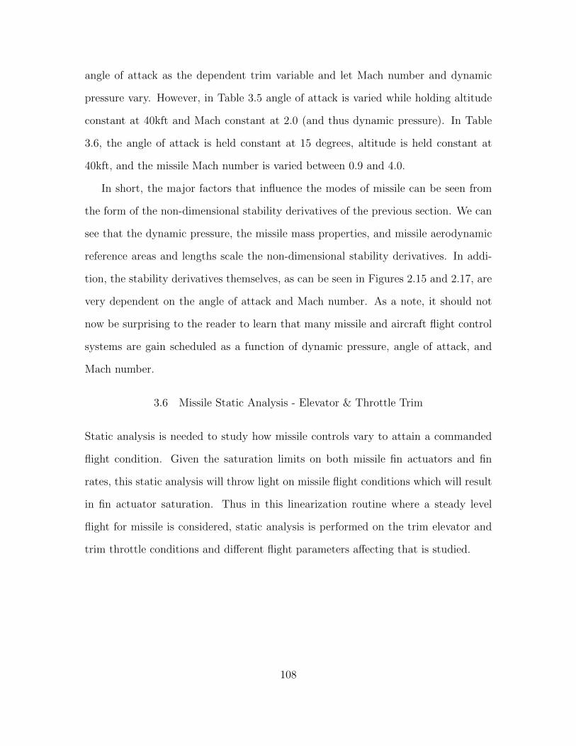
angle of attack as the dependent trim variable and let Mach number and dynamic
pressure vary. However, in Table 3.5 angle of attack is varied while holding altitude
constant at 40kft and Mach constant at 2.0 (and thus dynamic pressure). In Table
3.6, the angle of attack is held constant at 15 degrees, altitude is held constant at
40kft, and the missile Mach number is varied between 0.9 and 4.0.
In short, the major factors that influence the modes of missile can be seen from
the form of the non-dimensional stability derivatives of the previous section. We can
see that the dynamic pressure, the missile mass properties, and missile aerodynamic
reference areas and lengths scale the non-dimensional stability derivatives. In addi-
tion, the stability derivatives themselves, as can be seen in Figures 2.15 and 2.17, are
very dependent on the angle of attack and Mach number. As a note, it should not
now be surprising to the reader to learn that many missile and aircraft flight control
systems are gain scheduled as a function of dynamic pressure, angle of attack, and
Mach number.
3.6 Missile Static Analysis - Elevator & Throttle Trim
Static analysis is needed to study how missile controls vary to attain a commanded
flight condition. Given the saturation limits on both missile fin actuators and fin
rates, this static analysis will throw light on missile flight conditions which will result
in fin actuator saturation. Thus in this linearization routine where a steady level
flight for missile is considered, static analysis is performed on the trim elevator and
trim throttle conditions and different flight parameters affecting that is studied.
108

10 20 30 40 50 606
8
10
12
14
16
18
20Level Flight − Elevator Trim at Mach = 2
Altitude (kft)
δ e (de
g)
α = 8 degα = 9 degα = 10 degα = 11 deg
Figure 3.43: Level Flight - Elevator Trim for Altitude
6 6.5 7 7.5 8 8.5 9 9.5 100
2
4
6
8
10
12
14
16
18Level Flight − Elevator Trim at Mach = 2
α (deg)
δ e (de
g)
Altitude = 5 kftAltitude = 10 kftAltitude = 20 kftAltitude = 30 kftAltitude = 40 kft
Figure 3.44: Level Flight - Elevator Trim for α
109

0 500 1000 1500 2000 25000.5
1
1.5
2
2.5
3
3.5
4Level Flight − Throttle Trim at α = 5 deg
Thrust (lbf)
Mac
h
Altitude = 5 kftAltitude = 10 kftAltitude = 20 kftAltitude = 30 kft
Figure 3.45: Level Flight - Throttle Trim
0.5 1 1.5 2 2.5 3 3.5 40
500
1000
1500
2000
2500Level Flight − Throttle Trim at α = 5 deg
Mach
Thr
ust (
lbf)
Altitude = 5 kftAltitude = 10 kftAltitude = 20 kftAltitude = 30 kft
Figure 3.46: Level Flight - Throttle Trim for Mach
110
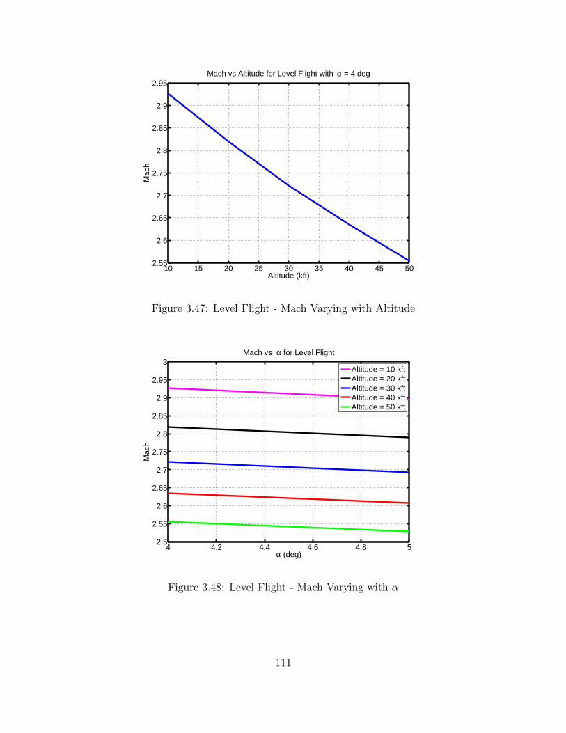
10 15 20 25 30 35 40 45 502.55
2.6
2.65
2.7
2.75
2.8
2.85
2.9
2.95Mach vs Altitude for Level Flight with α = 4 deg
Altitude (kft)
Mac
h
Figure 3.47: Level Flight - Mach Varying with Altitude
4 4.2 4.4 4.6 4.8 52.5
2.55
2.6
2.65
2.7
2.75
2.8
2.85
2.9
2.95
3Mach vs α for Level Flight
α (deg)
Mac
h
Altitude = 10 kftAltitude = 20 kftAltitude = 30 kftAltitude = 40 kftAltitude = 50 kft
Figure 3.48: Level Flight - Mach Varying with α
111

10 10.5 11 11.5 12 12.5 134
4.1
4.2
4.3
4.4
4.5
4.6
4.7
4.8α vs Altitude for Level Flight with Mach = 2.9
α (d
eg)
Altitude (kft)
Figure 3.49: Level Flight - α Varying with Altitude
From figure 3.43, it is clear that when a rise in altitude is demanded, the elevator
deflection increases. Also when positive angle of attack is commanded, the elevator
fin deflection increases. This is expected because, elevator deflection is responsible
for the missile to pitch up or down. While positive elevator deflection pitches up
the missile to match the commanded angle of attack or altitude, negative deflection
does the opposite. Interesting point to note here is the fin saturation level. If higher
angle of attack or altitude is commanded, elevator deflection saturates. While a lin-
ear behaviour is exhibited by the fin deflection with respect to change in altitude
and angle of attack, the same behaviour is lost and saturation occurs beyond cer-
tain commanded values. This is very much evident from the figure 3.43. Thus given
this detailed analysis, one should not command more than some threshold angle of
attack or altitude values as fin deflections will saturate beyong those threshold values.
From Figures 3.47, 3.48 & 3.49 respectively, the following concepts are very evident.
112

1. Mach ∝ 1h
2. Mach ∝ 1α
3. h ∝ α
3.7 Summary and Conclusions
In this chapter, mathematical modeling of a BTT missile was discussed. Modeling
included linearization routine using perturbation technique and time scaling. Both
lateral and longitudinal models were presented in detail. The nonminimum phase ze-
ros and unstable poles in both longitunal and lateral dynamics were analyzed in detail.
Finally the missile static analysis was performed for elevator trim and throttle trim
conditions and effect of various flight parameters on fin saturations was presented.
113

Chapter 4
MISSILE SEEKER / NAVIGATION & GUIDANCE
4.1 Introduction and Overview
This chapter describes the seeker/navigation system dynamics and the three guid-
ance options available to the missile. Navigation is traditionally defined as knowing
the location of a missile [62]. This is essential in long distance applications such as
inter-Continental Ballistic Missiles (ICBMs). For EMRAAT missile being considered,
navigation involves using range and range-rate information to determine where it is
with respect to its target. Hence, in this document, the term navigation is used to
refer to the missile determining its location with respect to the target.
A seeker is a range and angle sensing instrument which resides in the forward
portion of the missile. It provides the guidance system with information about the
evading target. The gimbals isolate the gyros from the missile’s rotational environ-
ment, as explained in [60]. The seeker/navigation system can be visualized as shown
in the Figure 4.1. It consists of a (1) Relative Range/Rate Generator, (2) LOS Angle
Generator, (3) A/D Quantizing block, (4) Gimbal Angle/Rate Error Generator and
a (5) Gimbal Rate Generator. Each subsystem is described in this chapter. The next
section describes the seeker/navigation system in greater detail.
The missile guidance systen processes range and range-rate information from the
seeker / navigation system and generates commanded horizontal and vertical accel-
erations to the autopilot. Three guidance laws are available to the missile.
114
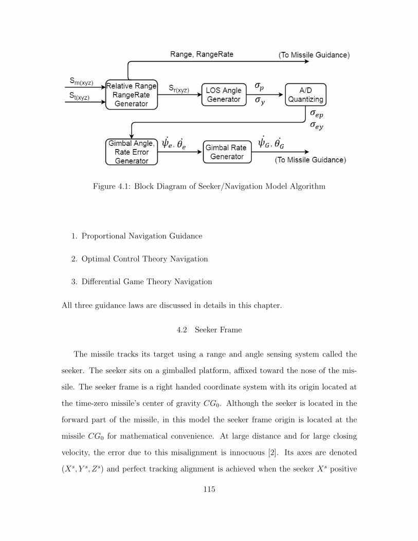
Figure 4.1: Block Diagram of Seeker/Navigation Model Algorithm
1. Proportional Navigation Guidance
2. Optimal Control Theory Navigation
3. Differential Game Theory Navigation
All three guidance laws are discussed in details in this chapter.
4.2 Seeker Frame
The missile tracks its target using a range and angle sensing system called the
seeker. The seeker sits on a gimballed platform, affixed toward the nose of the mis-
sile. The seeker frame is a right handed coordinate system with its origin located at
the time-zero missile’s center of gravity CG0. Although the seeker is located in the
forward part of the missile, in this model the seeker frame origin is located at the
missile CG0 for mathematical convenience. At large distance and for large closing
velocity, the error due to this misalignment is innocuous [2]. Its axes are denoted
(Xs, Y s, Zs) and perfect tracking alignment is achieved when the seeker Xs positive
115

axis passes through the target’s position. Seeker gimbal angles (ψs, θs, 0) represent
the measured azimuth and elevation of the seeker frame relative to XbZb and XbY b
planes of the body frame. This orientation of the seeker platform relative to the body
frame is shown in Figure 4.2. The seeker frame is used to describe error between
the actual flight path and the desired flight path. Vectors are transformed between
the seeker and body frames by transformation matrices which use the seeker gimbal
angles (ψs, θs, 0)s.
Figure 4.2: Seeker Frame orientation with respect to Seeker Gimbal Angles
A polar form of the target position in the seeker frame is given by components of
radial distance Range and seeker line-of-sight angles (σy, σp) as shown in the Figure
4.3, where line-of-sight is defined as the distance from the missile center-of-gravity to
the target center-of-gravity. σy corresponds t the azimuth angle and σp corresponds
to the elevation angle. These angles are calculated as a function of the seeker frame
116

Figure 4.3: Seeker Frame Line-of-Sight Angles (σy, σp) and Range
representation of the vehicle relative displacement Srv. The vehicle realtive vector
Srv identified as Ss
s in the seeker frame, is found by the following equation:
Sss = [Tbs][Tvb]Sr
v (4.1)
The 3×3 vehicle-to-body transformation matrix, denoted by Tvb is given by the
following equations. To transform a vector from body frame to the vehicle frame, the
transposed matrix Tvb′
is used.
Ax
Ay
Az
body
= Tvb
Ax
Ay
Az
vehicle
(4.2)
Tvb =
cos(θ) cos(ψ) cos(θ) sin(ψ) − sin(θ)
sin(θ) cos(ψ) sin(φ)− sin(ψ) cos(φ) sin(θ) sin(ψ) sin(φ)− cos(ψ) cos(φ) cos(θ) sin(φ)
sin(θ) cos(ψ) cos(φ) + sin(ψ) sin(φ) sin(θ) sin(ψ) sin(φ)− cos(ψ) sin(φ) cos(θ) cos(φ)
(4.3)
117

The 3×3 body-to-seeker transformation matrix, denoted by Tbs is given by the
following equations. To transform a vector from the seeker frame to the body frame,
the transposed matrix Tbs′
is used.
Ax
Ay
Az
seeker
= Tbs
Ax
Ay
Az
body
(4.4)
Tbs =
cos(θs) cos(ψs) cos(θs) sin(ψs) sin(θs)
sin(ψs) cos(ψs) 0
sin(θs) cos(ψs) sin(θs) sin(ψs) cos(θs)
(4.5)
The seeker LOS angles are then found by:
σy = tan−1
(SsySsx
)(4.6)
and:
σp = tan−1
−Ssz√Ssx
2 + Ssy2
(4.7)
4.3 Seeker Dynamics
The following section describes how the missile tracks its target. the seeker refer-
ence frame is used to describe error between desired and actual missile flight path.
4.3.1 Seeker Model Software Algorithm
This section describes how the seeker dynamics are modelled in the software. Each
of the blocks in the Figure 4.1 are now described.
118

Relative Range Rate Generator
A definition is definitely needed to conveniently describe the distance between the
missile and target. The vehicle separation is found as the difference between the
inertial frame target position and the inertial frame missile position. The calculations
in block one, see Figure 4.1 are described by the following equations. The relative
separation is defned as follows:
Srv def
= Sti − Smi (4.8)
with components
Srv = (Srx , Sry , Srz) (4.9)
The relative velocity is defined as follows:
Vrv def
= Vti − Vmi (4.10)
with components
Vrv = (Vrx , Vry , Vrz) (4.11)
The vehicle relative separation can be visualized as shown in the Figure 4.4.
LOS Angle Generator
To find the perfect Line-of-sight (LOS) angles, σy and σp, the relative target infor-
mation is transformed first from the relative frame into the body frame and then into
the seeker frame. The seeker LOS angles are then found by:
σy = tan−1
(SsySsx
)(4.12)
119
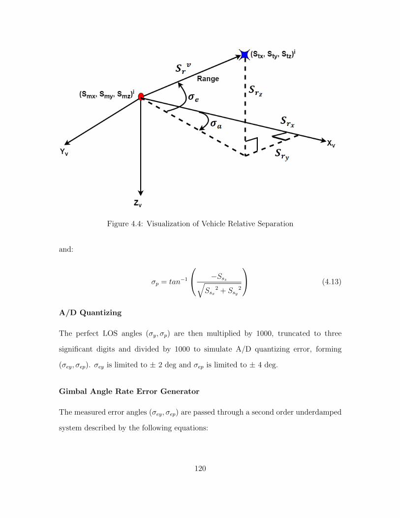
Figure 4.4: Visualization of Vehicle Relative Separation
and:
σp = tan−1
−Ssz√Ssx
2 + Ssy2
(4.13)
A/D Quantizing
The perfect LOS angles (σy, σp) are then multiplied by 1000, truncated to three
significant digits and divided by 1000 to simulate A/D quantizing error, forming
(σey, σep). σey is limited to ± 2 deg and σep is limited to ± 4 deg.
Gimbal Angle Rate Error Generator
The measured error angles (σey, σep) are passed through a second order underdamped
system described by the following equations:
120

ψe + 2ζsωsψe + ω2sψe = ω2
sσey (4.14)
θe + 2ζsωsθe + ω2sθe = ω2
sσep (4.15)
where ζsdef= is the damping ratio of the seeker servos and is equal to 0.35
ωsdef= is the servo natural frequency of oscillation and is equal to 49.5 ( rad
sec)
The seeker gimbal yaw and pitch error angles (ψe, θe) and their rates (ψe, θe) are taken
as the output of the underdamped system. this is given in state space form by the
following matrix equations. The state equations equivalent to the yaw axis equation
is given by:
ψeψe
=
0 1
−ωs2 −2ζsωs
ψeψe
+
0
ωs2
[σey] (4.16)
The state equations equivalent to the yaw axis equation is given by:
θeθe
=
0 1
−ωs2 −2ζsωs
θeθe
+
0
ωs2
[σep] (4.17)
Gimbal Rate Generator
Figure 4.5: Commanded Gimbal Rate Generator
121

The gimbal error angles and rates are scaled using:
ψG = ψe + 30ψe (4.18)
θG = θe + 30θe (4.19)
and limited by:
|ψGsat| < 75deg
sec= ψGmax (4.20)
|θGsat| < 75deg
sec= θGmax (4.21)
to form commanded gimbal rates (ψGsat , θGsat). Figure 4.5 shows a block diagram of
the scale and limit process.
Gimbal angles (ψG, θG) are found by the following equations:
ψG =
∫ψG − (P,Q,R)s (4.22)
θG =
∫θG − (P,Q,R)s (4.23)
where (P,Q,R)s represents the missile angular velocities transformed into the seeker
frame.
The servo deflections are limited in position to:
ψGmax = ±65deg (4.24)
θGmax = ±70deg (4.25)
The navigation seeker model simulates A/D quantization error as described above. It
would also be desirable to introduce noise in the relative displacement calculations.
122
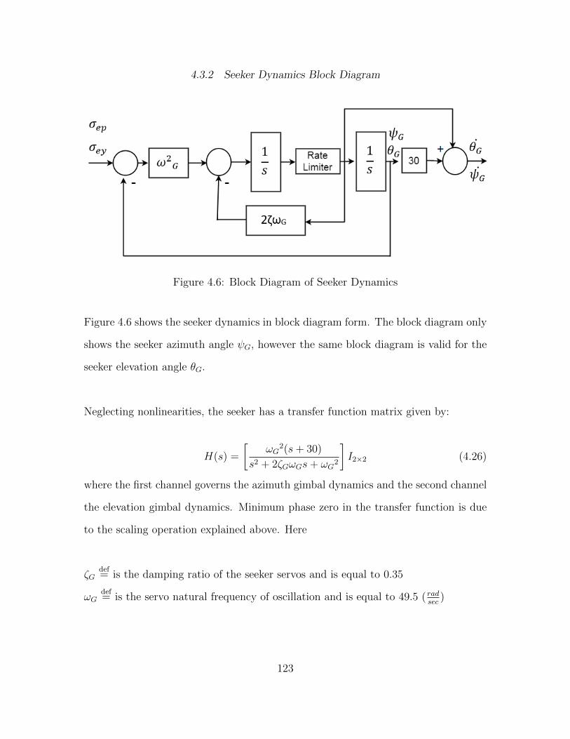
4.3.2 Seeker Dynamics Block Diagram
Figure 4.6: Block Diagram of Seeker Dynamics
Figure 4.6 shows the seeker dynamics in block diagram form. The block diagram only
shows the seeker azimuth angle ψG, however the same block diagram is valid for the
seeker elevation angle θG.
Neglecting nonlinearities, the seeker has a transfer function matrix given by:
H(s) =
[ωG
2(s+ 30)
s2 + 2ζGωGs+ ωG2
]I2×2 (4.26)
where the first channel governs the azimuth gimbal dynamics and the second channel
the elevation gimbal dynamics. Minimum phase zero in the transfer function is due
to the scaling operation explained above. Here
ζGdef= is the damping ratio of the seeker servos and is equal to 0.35
ωGdef= is the servo natural frequency of oscillation and is equal to 49.5 ( rad
sec)
123

Servo deflections are limited in position 1.
4.4 Guidance Algorithms
The missile guidance makes corrections to keep the missile on course by send-
ing appropriate acceleration commands to the autopilot [62], see Figure 1.1. Missile
Commanded horizontal and vertical body-frame accelerations Ayc and Azc are gen-
erated from measured relative target range and range-rate. Three guidance laws are
available to the missile autopilot. They are,
1. Proportional Navigation Guidance
2. Optimal Control Theory Navigation
3. Differential Game Theory Navigation [3]
4.4.1 Proportional Navigation Guidance
Figure 4.7: Proportional Navigation Guidance
The proportional guidance as shown in Figure 4.7 can be mathematically described
by the following equations.
Ayc = −pg1 RangeRate ψG (4.27)
Azc = pg2 RangeRate˙θG (4.28)
1Not Shown in block diagram. See code in Appendix A.
124

where Ayc and Azc are in the directions of the body frame axis Y b and Zb respectively.
The proportional navigation gains are summarized in Table 4.1:
pg1 = 3.0
pg2 = 3.0
Table 4.1: Proportional Guidance Gains
For proportional guidance, the missile is commanded to turn at a rate proportional
to the angular velocity of the line-of-sight. If the proportional guidance gains, pg1 and
pg2 are small, the missile will respond slowly and it will not be able to catch the target.
If the gains are too large the (outer) guidance loop will become unstable due to the
high frequency seeker dynamics, see [62].
4.4.2 Optimal Control Theory Guidance
The optimal guidance shown in Figure 4.8 can be described using the following
equations.
Figure 4.8: Optimal Control Theory Guidance
125

Body Frame Displacement Generator
The relative position and relative velocity along he missile Xv axis are transformed
into the body frame using the vehicle reference to body transformation matrix, shown
in Chapter 2.
Sxb = TvbSx
v (4.29)
Vxb = TvbVx
v (4.30)
Time-to-go Estimator
This outputs a guidance law time-to-go estimate that forces missile’s axial acceleration
command to be current acceleration.
Acurr = Vxb2 + Ax
bSxb (4.31)
If the current acceleration is not zero, time-to-go, denoted as Tgo is established as
Tgo =2Sx
b
√Acurr − Vxb
(4.32)
Otherwise, the time-to-go is
Tgo = −Sxb
Vxb
(4.33)
Relative Frame Acceleration Generator
The inertial acceleration commands are computed from missile relative positions and
velocities as follows
126

Axi = K1
(SrxTgo
+ Vrx
)Tgo
(4.34)
Ayi = K1
(SryTgo
+ Vry
)Tgo
(4.35)
Azi = K1
(SrzTgo
+ Vrz
)Tgo
− g (4.36)
where, g is defined in Equation (2.47).
Body Frame Acceleration Generator
The vehicle reference to body transformation matrix is used to transform commanded
inertial frame acceleration (Ayi, Az
i) into missile body commands (Ayc, Azc).
4.4.3 Differential Game Theory Guidance
In such formulations, a disturbance (e.g. Target Maneuver) “competes” with a
control (e.g. missile acceleration command). The disturbance attempts to maximize
a performace index (e.g. Miss Distance), while the control attempts to minimize the
index [61]. Maneuver Index is a unit-less quantity which is used to quantify the degree
of maneuverability of the target [19]. The differential game theory guidance is a vari-
ation of the optimal guidance. The commanded accelerations are first found from the
optimal guidance algorithm, denote them (Ayco, Azco). The differential game theory
guidance commanded accelerations are then found using the following equations:
Ayc =Ayco
1−MI(4.37)
Azc =Azco
1−MI(4.38)
MI is defined as a Maneuver Index constant.
127

The missile autopilot receives the acceleration commands (Amy, Amz) from the
guidance system and converts them into fin deflection commands in order to steer the
missile.
4.5 Summary and Conclusions
In this chapter, the seeker/navigation system dynamics were described. A block
diagram of the seeker dynamics was given to show how the commanded seeker servo
angles are generated. Also, the seeker model software algorithm was described. The
missile guidance system, which processes range and range-rate infromation from the
seeker/navigation system, was described. the guidance system generated commanded
horizontal and vertical body accelerations to the autopilot. The three guidance algo-
rithms available in this simulation were also discussed. Guidance algorithms included:
proportional, optimal and differential game theory.
128

Chapter 5
TARGET MODELING
5.1 Introduction and Overview
This chapter gives a description of the three-degree-of-freedom target model and
the three evasive maneuvers available to the target. For more on the target models
used in this simulations, the reader is referred to [3] and [4]. For more on target
modeling, in general, the reader is referred to [18], [52], [60].
A simple evasive three-degree-of-freedom target model is included in the program
to test the missile’s tracking and steering capabilities. The model used to describe
the target dynamics is discussed in Section 5.2. The target can be made to maneuver
with one of three methods. The target can fly straight with no evasive accelerations,
use the Sheldon turn and climb methods [4] or use the Rigges Vergaz turn and dive
method [3].
5.2 3DOF Target Dynamics
The target used in this study is modeled as a point mass with three degrees of
freedom. The following vector differential equation is used to describe the target’s
response to acceleration commands:
At =(Atc − At)
τ(5.1)
where
Atdef= actual target body acceleration, (Atx , Aty , Atz)
i
129

Atcdef= commanded acceleration, (Ayc, Azc)
τdef= response time-constant and is = 0.5
The commanded acceleration, Atc is a function of: estimated time to go, and (sin,
cos) of missile Euler (yaw, pitch, roll) angles. Commanded accelerations are restricted
to a range representing the limits of a pilot’s mental alertness, ±9G’s.
5.3 Straight Flight with No Maneuver.
The simplest option available to the target is to make it to fly in a straight path
with constant velocity. No evasive maneuvers are generated to avoid the oncoming
missile. The commanded target acceleration, Atc = (Atxc , Atyc , Atzc)i is determined
using the following algorithm:
Algorithm:
Compute the target inertial acceleration, Atc as:
Atxc = 0
Atyc = 0
Atzc = 0
5.4 Sheldon Turn & Climb Maneuver
The Sheldon Turn & Climb algorithm can be visualized as in Figure 5.1; viewed
from the target toward the missile. For missile position in the right half of the target
plane-of-view, the target will turn and climb right. If the missile lies in the left half
of the target plane-of-view, the target will turn and climb left.
130

Figure 5.1: Sheldon Evasive Maneuver, Viewed from target-to-missile.
The commanded target inertial acceleration, Atc is calculated using time-to-go
information from the missile autopilot, target Euler angles and the initial missile-
target Aspect angle. The aspect angle measures angle from the inertial LOS vector
to target velocity vector. The target euler angles are defined identically to the missile
Euler angles in Chapter 2. For more on the Sheldon Turn & Climb algorithm, reader
is referred to [4]. The commanded target acceleration Atc is determined using the
following algorithm.
Algorithm:
1. Calculate sine and cosine of commanded target Euler roll angle φ based on
estimated time-to-go and initial Aspect angle. Also, assign a value to Ant the
desired target normal acceleration. g0 is defined in Chapter 2.
If time-to-go > 1, then sin(φ) = 0.707 sign of (sin(Aspect)), cos(φ) = 0.707 and
Ant = 5 g0
Else sin(φ) = 0, cos(φ) = 0.707 and Ant = 9 g0
2. Calculate target total body velocity as Vt =√
[Vtx2 + Vty
2 + Vtz2]
3. Calculate target body velocity in X iY i plane as Vtxy =√
[Vtx2 + Vty
2]
131

4. Limit desired normal acceleration as a function of local air density (ρ) and Vt,
so target angle of attack, α remains < 30 deg, i.e. 0.0 < At < 0.33 ρ Vt
5. Calculate sine and cosine target Euler pitch angle. sin(θ) = −VtzVt
and cos(θ) =
VtxyVt
6. Calculate sine and cosine target Euler yaw angle. sin(ψ) =−VtyVtxy
and cos(ψ) =
VtxVtxy
7. Compute target inertial acceleration, Atc , where g is as defined in Chapter 2.
(a) Atxc = -Ant (cos(φ) sin(θ) cos(ψ) + sin(φ) sin(ψ))
(b) Atyc = -Ant (cos(φ) sin(θ) sin(ψ)− sin(φ) cos(ψ))
(c) Atzc = -Ant (cos(φ) cos(θ)) - g
5.5 Riggs Vergaz Turn & Dive Maneuver
The Riggs Vergaz Turn & Dive algorithm can be visualized as in Figure 5.2; viewed
from target-to-missile. Missile may be spotted in one of the four quadrants. Missile
positions in the bottom(top) two halves of the target plane-of-view result in the target
turning and climbing(diving) right or left as indicated.
132

Figure 5.2: Riggs Vergaz Evasive Maneuver, Viewed from target-to-missile.
For more on the Riggs Vergaz Turn & Dive algorithm, reader is referred to [3].
The commanded target acceleration Atc is determined using the following algorithm.
Algorithm:
1. Calculate sine and cosine of commanded target Euler roll angle φ based on
estimated time-to-go and initial Aspect angle. Also, assign a value to Ant the
desired target normal acceleration. g0 is defined in Chapter 2.
If time-to-go > 1, then sin(φ) = 0.707 sign of (sin(Aspect)), cos(φ) = -0.707 sign
of (sin(Aspect)) and Ant = 9 g0
Else sin(φ) = 0, cos(φ) = -1 and Ant = 9 g0
2. Calculate target total body velocity as Vt =√
[Vtx2 + Vty
2 + Vtz2]
3. Calculate target body velocity in X iY i plane as Vtxy =√
[Vtx2 + Vty
2]
4. Limit desired normal acceleration as a function of local air density (ρ) and Vt,
so target angle of attack, α remains < 30 deg, i.e. 0.0 < At < 0.33 ρ Vt
133

5. Calculate sine and cosine target Euler pitch angle, sin(θ) = −VtzVt
and cos(θ) =
VtxyVt
6. Calculate sine and cosine target Euler yaw angle, sin(ψ) =−VtyVtxy
and cos(ψ) =
VtxVtxy
7. Compute target inertial acceleration, Atc , where g is as defined in Chapter 2.
(a) Atxc = -Ant (cos(φ) sin(θ) cos(ψ) + sin(φ) sin(ψ))
(b) Atyc = -Ant (cos(φ) sin(θ) sin(ψ)− sin(φ) cos(ψ))
(c) Atzc = -Ant (cos(φ) cos(θ)) - g
5.6 Summary and Conclusions
In this chapter, a 3 degree-of-freedom target model was described. The target
model is included in the program to test the missile’s tracking and steering capabil-
ities. Three target maneuver algorithms were discussed. Each algorithm has been
implemented in the simulation software. The target evasive maneuvers include: (1)
Straight Flight with No Maneuver, (2) the Sheldon Turn and Climb maneuver and
(3) the Riggs Vergaz Turn and Dive maneuver.
134

Chapter 6
BTT MISSILE AUTOPILOT
6.1 Introduction and Overview
In order to acheive adequate performance over the entire envelope of operating
conditions, the autopilot of modern air-to-air tactical missile must be nonlinear [10].
Because of the inherent instabilities associated with missiles, stability augmentation
systems are essential. The autopilot provides the added stability and ensures that
accelerations from the guidance systems are properly followed. More precisely, the
autopilot uses feedback to process the guidance commands and deliver appropriately
coordinated fin commands to the actuators.
Throughout this research, a BTT missile has been considered. BTT missile con-
trol is made more difficult by the high roll rates required to achieve the short response
time necessary for a high-performance missile. The high roll rates increase the aero-
dynamic coupling, which will be discussed here and can lead to inertial cross-coupling
problems. The motivation for using BTT missile control is that the ramjet missile
propulsion requires positive angles of attack and minimal sideslip angles, whch can
be achieved by BTT missiles.
The bank-to-turn steering policy used in this simulation is sometimes referred
to as Preferred Orientation Control (POC) [20]. In other words, it turns like an
airplane. The EMRAAT missile is asymmetrical, see Figures 6.1 and 6.2, making
the bank-to-turn steering policy particularly desirable. The propulsive performance
135

of asymmetric missiles or missiles with off-axis air-breathing propulsion systems [20]
may be adversely affected with certain angles of attack or sideslip. A bank-to-turn
steering policy provides minimum sideslip angle.
Figure 6.1: An Asymmetrical EMRAAT Missile
The guidance system sends horizontal and vertical acceleration commands to the
autopilot. The commands are processed and converted into appropriately coordinated
fin commands which are delivered to the actuators.
Body acceleration commands (Ayc, Azc) generated by the guidance system are
converted by the autopilot into commanded fin deflection angles F1c, F2c, F3c and
F4c. The autopilot consists of following components:
1. Acceleration-Roll-Side-Slip Command Generator (BTT LOGIC)
2. Angular Rate Command Generator
3. Mixed Fin Command Generator: p-q-r-thrust/drag
136

Figure 6.2: An Asymmetrical EMRAAT Missile Dimesions
4. ILAAT De-Mixer: Four Fin Force Commands to Actuators
5. ILAAT Mixer: Three Effective Aileron, Flapperon, Rudder Controls
Fundamentally, the autopilot is a nonlinear gain scheduled controller designed
using classical control ideas. Two-loop autopilot structure is used here. Innermost
loop is used to control the rate dynamics which are faster and outer loop controls
the sideslip dynamics. BTT missiles ideally should have no Side-Slip. To achieve
a desired orientation, the missile is rolled(banked) so that the plane of maximum
aerodynamic normal force is oriented to the desired direction. Magnitude of the force
is then controlled by adjusting the angle of attack in that plane. Figure 6.3 shows
137

the information flow through the autopilot. Body acceleration commands (Ayc, Azc)
generated by the guidance system are converted by the autopilot into commanded
fin deflection angles F1c, F2c, F3c and F4c. Four tail-mounted fins steer the missile.
Effective roll, pitch and yaw deflection angles (δp, δq, δr) are algebraically related to
the fin deflection angles. Each component of the autopilot is described in this chapter.
If we are primarily interested in controlling the missile
then when does a need for nonlinear controller arises?
So when we want our missile to operate over an entire envelope of flight conditions,
the need for a nonlinear autopilot design arises. The gain of the controller should be
scheduled as function of flight conditions for operating across the entire envelope of
flight conditions. Thus the missile needs a nonlinear gain scheduled autopilot. There
are several ways of obtaining a nonlinear controller and one best technique is to use
Incremental Nonlinear Dynamic Inversion. The entire process is explained in detail
in this chapter.
Remainder of this chapter is organized as follows: Section 6.2 discusses the non-
linear dynamic inversion using feedback linearization technique to obtain a nonlinear
controller for the nonlinear missile plant. Also the design of controller gains as a func-
tion of flight condition(Gain Scheduling) is discussed in detail there. Then in Section
6.3, the BTT logic of designing for commanded bank angle for missile is discussed.
Fair amount of information is also provided about the singularity problem that arises
in the design and the ways to correct it. Section 6.4 explains how commanded angu-
lar rates are formed which serve as the reference for Innermost Angular Rate Control
Loop. In the Section 6.5, the design for the commanded control deflections from the
138

Figure 6.3: Block diagram of BTT Missile Autopilot
Figure 6.4: Determination of Commanded Roll Angle from Ayc & Azc
angular rate information is discussed. Section 6.6 throws light on how the commanded
control deflections combine together to form the commanded fin deflections. Section
6.7 explains how to realize the effective control deflections from fin deflections from
the actuators. The simulation results using the nonlinear gain scheduled autopilot is
presented in section 6.8. A comprehensive analysis of nonlinear autopilot is done in
139

Section 6.9 where the nonlinear autopilot is linearized and analyzed with the missile
linear plant design obtained from Chapter 3. Autopilot is analyzed for its robustness
and performance. Finally Section 6.10 concludes the work done in this chapter.
6.2 Control Law Formulation
The control law used in this research is obtained through Incremental Nonlinear
Dynamic Inversion (INDI) using feedback linearization technique [69]. To apply NDI
technique, it is required to know the full state of the system. If the state is not
known, they can be approximated using nonlinear observer or stochastic state esti-
mator as required. Also the system model has to be known completely to cancel the
nonlinearities. If the system model is partially known, system identification process
has to be done to get a full model knowledge. However system possessing RHP zeros
(nonminimum phase systems) are not a good candidate for the application of NDI
technique to obtain a nonlinear controller. The RHP zero-dynamics will result in a
unstable controller while being inverted to cancel the nonlinearities. Missile accel-
eration control is a nonminimum phase problem. But when we assume symmetrical
airframe by neglecting the inertial cross-coupling elements, it results in a minimum
phase system and ready for NDI technique to be applied. The design of innermost
autopilot rate control is done as following.
Let us recall the rotational dynamics of missile involving inertial and rate components
as below L
M
N
com
= Jω + ω × Jω (6.1)
140
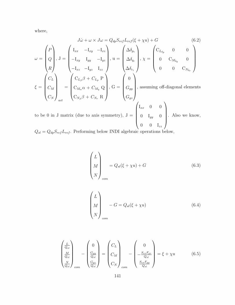
where,
Jω + ω × Jω = QdpSrefLref (ξ + χu) +G (6.2)
ω =
P
Q
R
, J =
Ixx −Ixy −Ixz
−Ixy Iyy −Iyz
−Ixz −Iyz Izz
, u =
∆δpc
∆δqc
∆δrc
, χ =
CLδp
0 0
0 CMδq0
0 0 CNδr
ξ =
CL
CM
CN
act
=
CLββ + CLp P
CMαα + CMq Q
CNββ + CNr R
, G =
0
Ggy
Ggz
, assuming off-diagonal elements
to be 0 in J matrix (due to axis symmetry), J =
Ixx 0 0
0 Iyy 0
0 0 Izz
. Also we know,
Qsl = QdpSrefLref . Performing below INDI algebraic operations below,
L
M
N
com
= Qsl(ξ + χu) +G (6.3)
L
M
N
com
−G = Qsl(ξ + χu) (6.4)
LQsl
MQsl
NQsl
com
−
0
GgyQsl
GgzQsl
=
CL
CM
CN
com
−
0
−ScxFgzQsl
ScxFgyQsl
= ξ + χu (6.5)
141
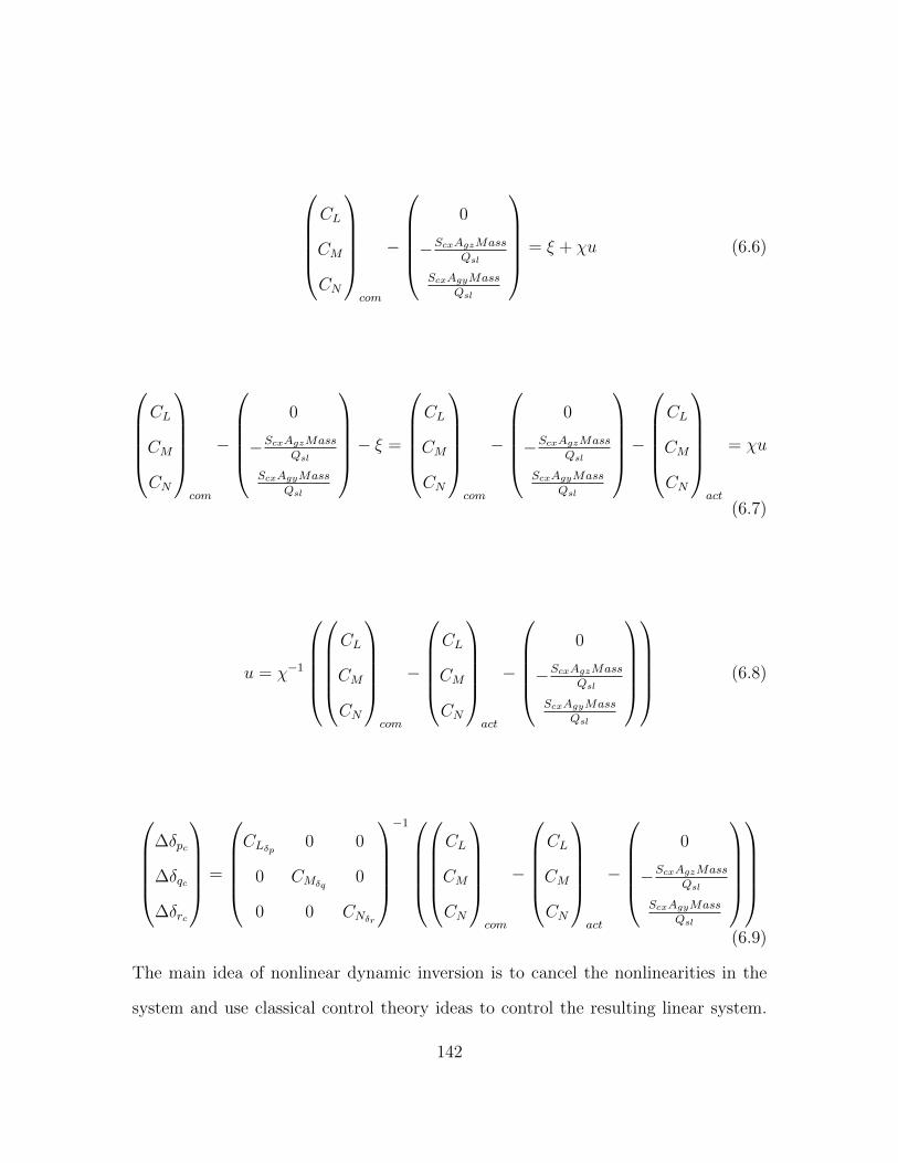
CL
CM
CN
com
−
0
−ScxAgzMass
Qsl
ScxAgyMass
Qsl
= ξ + χu (6.6)
CL
CM
CN
com
−
0
−ScxAgzMass
Qsl
ScxAgyMass
Qsl
− ξ =
CL
CM
CN
com
−
0
−ScxAgzMass
Qsl
ScxAgyMass
Qsl
−CL
CM
CN
act
= χu
(6.7)
u = χ−1
CL
CM
CN
com
−
CL
CM
CN
act
−
0
−ScxAgzMass
Qsl
ScxAgyMass
Qsl
(6.8)
∆δpc
∆δqc
∆δrc
=
CLδp 0 0
0 CMδq0
0 0 CNδr
−1
CL
CM
CN
com
−
CL
CM
CN
act
−
0
−ScxAgzMass
Qsl
ScxAgyMass
Qsl
(6.9)
The main idea of nonlinear dynamic inversion is to cancel the nonlinearities in the
system and use classical control theory ideas to control the resulting linear system.
142

So, the below 2 questions are very intuitive to ask.
1. How does the resulting linear system look like?
2. Is it still dependent upon flight conditions?
The following calculation will answer the above questions. Considering the 1st chan-
nel and referring to the equation 3.29, the following analysis can be made. Similar
procedures can be utilized for understanding the other 2 channels.
P =L
I∗xx=CLQdpSrefLref
I∗xx=QdpSrefLref
I∗xx(CLδpδp + CLPL2V P + CLββ) (6.10)
Rearranging above terms and writing as below,
P =QdpSrefLref
I∗xx
(CLPL2V P + CLββ
)+QdpSrefLref
I∗xx
(CLδpδp
)(6.11)
This now resembles standard nonlinear state equation as shown below,
P = f(P, β) + g(x)δp, which looks like, x = f(x) + g(x)u (6.12)
Substituting the control law obtained above from nonlinear dynamic inversion, we
get
P =QdpSrefLref
I∗xx
(CLδp
(K4(Pc − P )
Qdp
+CLβCLδp
(βc − β)
)+ CLPL2V P + CLββ
)(6.13)
Rearranging above terms writing in terms of varying coefficients & remembering that
βc is always set to zero, we get,
P = −g1 P + g2 Pc (6.14)
143
This looks like the following equation, with states, x = [P] and reference, r = [Pc]
x = −A(σ)x+B(σ) r (6.15)
6.2.1 Gain Scheduling of Linear Parameter Varying System
The equation 6.14 looks like a linear parameter varying system, where the “A” &
“B” matrices depend upon the flight conditions such as α, β, Mach & Qdp which are
collectively represented by σ scheduling variable. In designing feedback controllers
for dynamical systems, the controllers are often designed at various operating points
using linearized models of the system dynamics and are scheduled as a function of
a parameter or parameters for operation at intermediate conditions [74]. It is an
approach for the control of nonlinear systems that uses a family of linear controllers,
each of which provides satisfactory control for a different operating point of the sys-
tem. One or more observable variables, called the scheduling variables, are used to
determine the current operating region of the system and to enable the appropriate
linear controller. Here in case of BTT missile control, a set of controllers are designed
at different gridded locations of corresponding parameters such as α, β, Mach & δq.
In brief, gain scheduling is a control design approach that constructs a nonlinear con-
troller for a nonlinear plant by patching together a collection of linear controllers.
These linear controllers are blended in real-time via interpolation in our case through
the use of look up tables. Though the stability is not guaranteed at operating condi-
tions other than the design points, it is a very efficient technique where the parameter
dependency of controllers are large due to increased operating envelopes with more
demanding performance requirements.
Thus referring to 6.14, the system matrix depends upon α, Mach & Qdp. Essentially
144
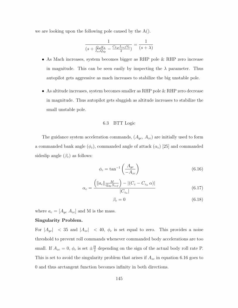
we are looking upon the following pole caused by the A().
1
(s+ QslK4
IxxQdp− CLP LrefVb
2)
=1
(s+ λ)
• As Mach increases, system becomes bigger as RHP pole & RHP zero increase
in magnitude. This can be seen easily by inspecting the λ parameter. Thus
autopilot gets aggressive as mach increases to stabilize the big unstable pole.
• As altitude increases, system becomes smaller as RHP pole & RHP zero decrease
in magnitude. Thus autopilot gets sluggish as altitude increases to stabilize the
small unstable pole.
6.3 BTT Logic
The guidance system acceleration commands, (Ayc, Azc) are initially used to form
a commanded bank angle (φc), commanded angle of attack (αc) [25] and commanded
sideslip angle (βc) as follows:
φc = tan−1
(Ayc−Azc
)(6.16)
αc =
(‖ac‖ M
Qdp Sref
)− |(Cz − Czα α)|
|Czα |(6.17)
βc = 0 (6.18)
where ac = [Ayc Azc] and M is the mass.
Singularity Problem.
For |Ayc| < 35 and |Azc| < 40, φc is set equal to zero. This provides a noise
threshold to prevent roll commands whenever commanded body accelerations are too
small. If Azc = 0, φc is set ±Π2
depending on the sign of the actual body roll rate P.
This is set to avoid the singularity problem that arises if Azc in equation 6.16 goes to
0 and thus arctangent function becomes infinity in both directions.
145

6.4 Angular Rate Command Generator
Rotation rate commands (Pc, Qc, Rc) are formed from Ayc, Azc, φc, β, dynamic
pressure, missile velocity and missile mass using below equations. Pc and Rc are
selected to be proportional to φ and β respectively. Azc is limited, denoted as AzcL,
so that the magnitude of pitch acceleration command (Qc) has a maximum value
near α = 28 degrees. The maximum acceleration command, denoted by Amzmax is
calculated form the current dynamic pressure Qdp and missile mass, m(t) as follows:
Amzmax = 5.25Qdp
m(t)(6.19)
If |Azc| > Amzmax , then AzcL is set to Amzmax , else it is left equal to Azc. Below
equations compute the rotation rate commands. The autopilot gains are summarized
in Table 6.1.
Pc = K1(φc − φ) (6.20)
Qc = K2(AzcL − Amzb)
Qdp
− AzcLVb
(6.21)
Rc = K3(βc − β) (6.22)
It is to be noted here that, Amzb = QsmCz = Qsm (CNα(αc − α) + CNδq δq)
146

K1 7
K2 -10
K3 0.5
K4 500
K5 -1.75
K6 -1500
K7 -5000
Table 6.1: Autopilot Gains
6.5 Mixed Fin Command Generator: p-q-r-thrust/drag
The commanded effective fin deflections (δpc , δqc , δrc) model an ideal set of phys-
ical fin deflections which cause the missile to roll, pitch and yaw about its body axes
[20]. The effective squeeze mode δs represents a squeeze or speed-brake mode, which
is used to minimize the axial drag, i.e. no preferred roll, pitch or yaw is induced [20].
After generation of the rate commands (Pc, Qc, Rc), these are used along with
the true body rotation rates (P, Q, R), α, β, Qdp, missile mass as well as a few of
the aerodynamic coefficients to generate effective aileron, elevator and roll commands
(δpc , δqc , δrc)1 via the following nonlinear control law.
δpc =K4(Pc − P )
Qdp
+CLβCLδp
(βc − β) (6.23)
δqc = (K5 +K6
Qdp
)(Qc −Q) +CMα
CMδq
(αc − α) +AgzScxMass
QslCMδq
(6.24)
δrc =K7(Rc −R)
Qdp
+CNβCNδr
(βc − β) +30PQ− AgyScxMass
QslCNδr(6.25)
1As we would do for an aircraft
147

where,
Qsl = QdpSrefLref (6.26)
Fgy and Fgz are gravitational accelerations in the body frame and Qdp, Sref and
Lref are as defined in the Chapter 2. The gains K4, K5, K6 and K7 are given in Table
6.1. Also produced is a squeeze mode command δsc formed by taking above linear
combination of previous values of (F1C , F2C , F3C and F4C) using 2:
δsc = 0.25(F1C − F2C − F3C + F4C) (6.27)
6.6 ILAAT De-Mixer: Four Fin Force Commands to Actuators
Finally, effective fin deflection commands (δpc , δqc , δrc) and the effective squeeze mode
δs are transformed algebraically into true fin deflection commands (F1, F2, F3, F4)
using below ILAAT (Integrated Logic for Air-to-Air Technology) combination logic
[48] below. The BTT missile used here uses the “×” delta configuration ILAAT
mixing logic as below,
F1C
F2C
F3C
F4C
=
−1 +1 −1 +1
−1 +1 +1 −1
+1 +1 −1 −1
+1 +1 +1 +1
δpc
δqc
δrc
δsc
(6.28)
6.7 ILAAT Mixer: 3 Effective Aileron, Flapperon, Rudder Controls
Finally, the effective control deflections (δp, δq, δr) i.e. aileron, flapperon and
rudder can be realized using ILAAT mixing combination logic as follows,
2Here, the current value of δsc is found by the previous values of (F1C - F2C - F3C + F4C)
148

∆δp
∆δq
∆δr
∆δs
= 0.25
−1 −1 1 1
1 1 1 1
−1 1 −1 1
1 −1 −1 1
∆F1
∆F2
∆F3
∆F4
(6.29)
The above matrix is the inverse of the matrix in the equation ()6.28.
6.8 Nonlinear Autopilot Simulation Results
Table 6.2 shows the flight conditions considered for evaluating the performance of
the new improved nonlinear autopilot design.
Flight Parameter Value Flight Parameter Value
Missile Max. Accel. 80 g Initial Height -1000 ft
Initial Missile Mach 0.8999 Target Range 2000 ft
Initial Target Mach 0.8999 Missile Guidance Optimal Control
Target Maneuver Sheldon Aspect Angle 0 deg
Table 6.2: Flight Conditions for Nonlinear Autopilot Simulations
149
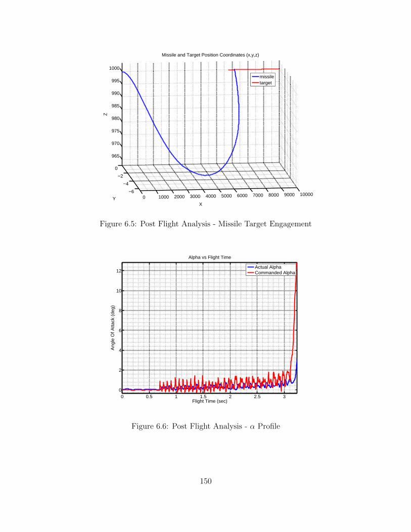
0 1000 2000 3000 4000 5000 6000 7000 8000 9000 10000−6
−4
−2
0
965
970
975
980
985
990
995
1000
Missile and Target Position Coordinates (x,y,z)
X
Y
Z
missiletarget
Figure 6.5: Post Flight Analysis - Missile Target Engagement
0 0.5 1 1.5 2 2.5 30
2
4
6
8
10
12
Alpha vs Flight Time
Flight Time (sec)
Ang
le O
f Atta
ck (
deg)
Actual AlphaCommanded Alpha
Figure 6.6: Post Flight Analysis - α Profile
150

0 0.5 1 1.5 2 2.5 3−0.1
−0.05
0
0.05
0.1
Beta vs Flight Time
Flight Time (sec)
Sid
eslip
Ang
le (
deg)
Actual SideslipCommanded Sideslip
Figure 6.7: Post Flight Analysis - β Profile
0 0.5 1 1.5 2 2.5 3
1000
2000
3000
4000
5000
6000
7000
8000
9000
10000Range vs Flight Time
Flight Time (sec)
Ran
ge (
ft)
Figure 6.8: Post Flight Analysis - Range Profile
151
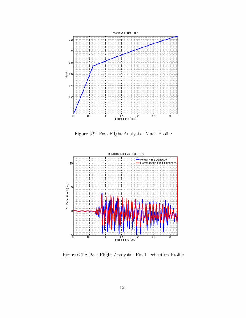
0 0.5 1 1.5 2 2.5 3
1
1.2
1.4
1.6
1.8
2
2.2
Mach vs Flight Time
Flight Time (sec)
Mac
h
Figure 6.9: Post Flight Analysis - Mach Profile
0 0.5 1 1.5 2 2.5 3−5
0
5
10
Fin Deflection 1 vs Flight Time
Flight Time (sec)
Fin
Def
lect
ion
1 (d
eg)
Actual Fin 1 DeflectionCommanded Fin 1 Deflection
Figure 6.10: Post Flight Analysis - Fin 1 Deflection Profile
152

0 0.5 1 1.5 2 2.5 3
−4
−2
0
2
4
6
8
10
12
Fin Deflection 2 vs Flight Time
Flight Time (sec)
Fin
Def
lect
ion
2 (d
eg)
Actual Fin 2 DeflectionCommanded Fin 2 Deflection
Figure 6.11: Post Flight Analysis - Fin 2 Deflection Profile
0 0.5 1 1.5 2 2.5 3
−4
−2
0
2
4
6
8
Fin Deflection 3 vs Flight Time
Flight Time (sec)
Fin
Def
lect
ion
3 (d
eg)
Actual Fin 3 DeflectionCommanded Fin 3 Deflection
Figure 6.12: Post Flight Analysis - Fin 3 Deflection Profile
153

0 0.5 1 1.5 2 2.5 3
−4
−2
0
2
4
6
Fin Deflection 4 vs Flight Time
Flight Time (sec)
Fin
Def
lect
ion
4 (d
eg)
Actual Fin 4 DeflectionCommanded Fin 4 Deflection
Figure 6.13: Post Flight Analysis - Fin 4 Deflection Profile
0 0.5 1 1.5 2 2.5 3−600
−400
−200
0
200
400
600Fin 1 Rate vs Flight Time
Flight Time (sec)
Fin
1 R
ate
(deg
/sec
)
Figure 6.14: Post Flight Analysis - Fin 1 Rate Profile
154

0 0.5 1 1.5 2 2.5 3−600
−400
−200
0
200
400
600Fin 2 Rate vs Flight Time
Flight Time (sec)
Fin
2 R
ate
(deg
/sec
)
Figure 6.15: Post Flight Analysis - Fin 2 Rate Profile
0 0.5 1 1.5 2 2.5 3−600
−400
−200
0
200
400
600Fin 3 Rate vs Flight Time
Flight Time (sec)
Fin
3 R
ate
(deg
/sec
)
Figure 6.16: Post Flight Analysis - Fin 3 Rate Profile
155

0 0.5 1 1.5 2 2.5 3−600
−400
−200
0
200
400
600Fin 4 Rate vs Flight Time
Flight Time (sec)
Fin
4 R
ate
(deg
/sec
)
Figure 6.17: Post Flight Analysis - Fin 4 Rate Profile
965 970 975 980 985 990 995 10002.308
2.3085
2.309
2.3095
2.31
2.3105
x 10−3 Air Density vs Missile Altitude
Missile Altitude (ft)
Air
Den
sity
(sl
ug/ft
3 )
Figure 6.18: Post Flight Analysis - Air Density Profile
156
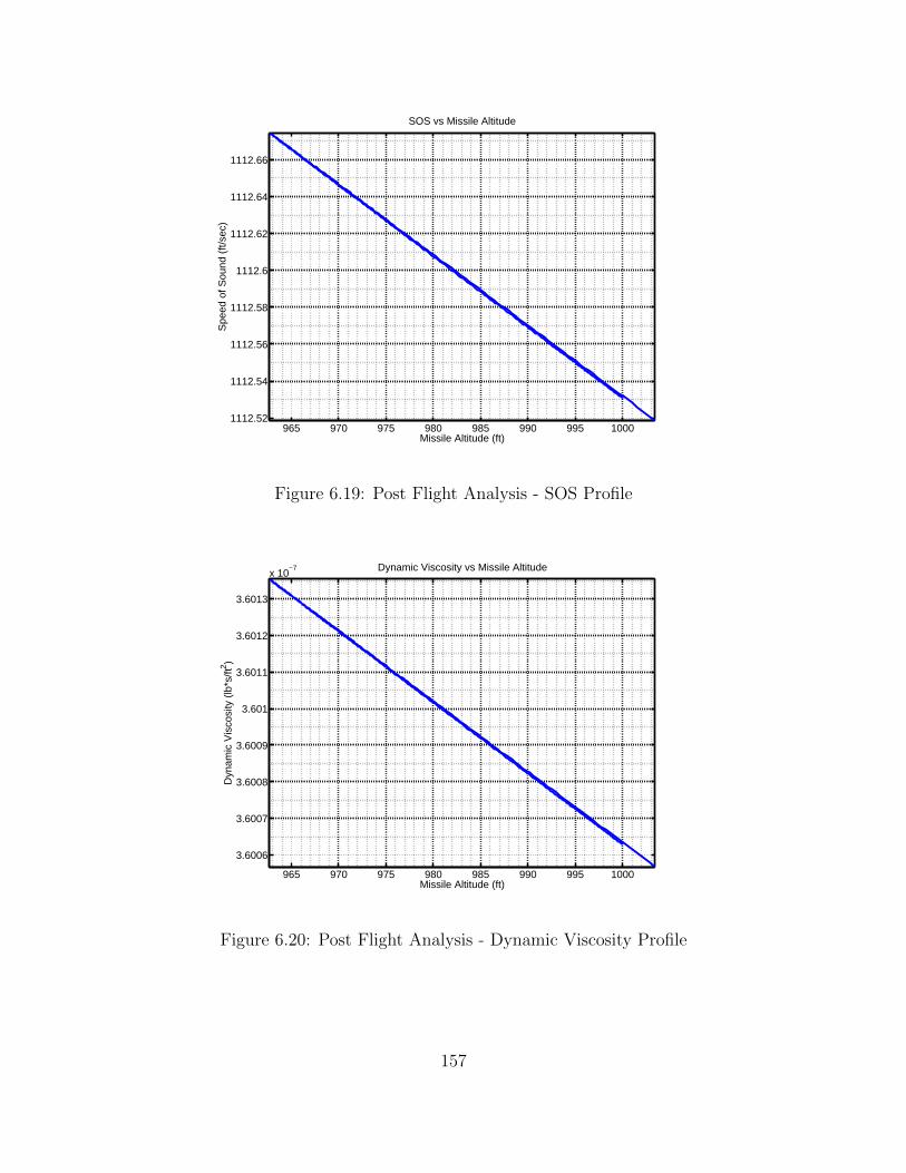
965 970 975 980 985 990 995 10001112.52
1112.54
1112.56
1112.58
1112.6
1112.62
1112.64
1112.66
SOS vs Missile Altitude
Missile Altitude (ft)
Spe
ed o
f Sou
nd (
ft/se
c)
Figure 6.19: Post Flight Analysis - SOS Profile
965 970 975 980 985 990 995 1000
3.6006
3.6007
3.6008
3.6009
3.601
3.6011
3.6012
3.6013
x 10−7 Dynamic Viscosity vs Missile Altitude
Missile Altitude (ft)
Dyn
amic
Vis
cosi
ty (
lb*s
/ft2 )
Figure 6.20: Post Flight Analysis - Dynamic Viscosity Profile
157

965 970 975 980 985 990 995 1000
1.5586
1.5588
1.559
1.5592
1.5594
1.5596
1.5598
1.56
x 10−4 Kinematic Viscosity vs Missile Altitude
Missile Altitude (ft)
Kin
emat
ic V
isco
sity
(lb
*s*f
t / s
lug)
Figure 6.21: Post Flight Analysis - Kinematic Viscosity Profile
0 0.5 1 1.5 2 2.5 3−80
−60
−40
−20
0
20
40
60
80
Ay and A
yc vs Flight Time
Flight Time (sec)
Ay (
g)
Actual Ay Acceleration
Commanded Ay Acceleration
Figure 6.22: Post Flight Analysis - Acceleration in Y Direction Profile
158

0 0.5 1 1.5 2 2.5 3−80
−60
−40
−20
0
20
40
60
80
Az and A
zc vs Flight Time
Flight Time (sec)
Az (
g)
Actual Az Acceleration
Commanded Az Acceleration
Figure 6.23: Post Flight Analysis - Acceleration in Z Direction Profile
0 0.5 1 1.5 2 2.5 3
−3
−2
−1
0
1
2
3
delP vs Flight Time
Flight Time (sec)
delP
(de
g)
delpdelp commanded
Figure 6.24: Post Flight Analysis - Aileron Profile
159

0 0.5 1 1.5 2 2.5 3
−2
0
2
4
6
8
delQ vs Flight Time
Flight Time (sec)
delQ
(de
g)
delqdelq commanded
Figure 6.25: Post Flight Analysis - Elevator Profile
0 0.5 1 1.5 2 2.5 3
−0.3
−0.25
−0.2
−0.15
−0.1
−0.05
0
0.05
0.1
0.15
0.2
delR vs Flight Time
Flight Time (sec)
delR
(de
g)
delrdelr commanded
Figure 6.26: Post Flight Analysis - Rudder Profile
160

0 0.5 1 1.5 2 2.5 3 3.5−4
−3
−2
−1
0
1
2
3
4Roll vs Flight Time
Flight Time (sec)
Rol
l ang
le (
deg)
Actual RollCommanded Roll
Figure 6.27: Post Flight Analysis - Roll Angle Profile
0 0.5 1 1.5 2 2.5 3 3.5−40
−30
−20
−10
0
10
20
30
40Roll Rate vs Flight Time
Flight Time (sec)
Rol
l Rat
e (d
eg/s
ec)
Actual Roll RateCommanded Roll Rate
Figure 6.28: Post Flight Analysis - Role Rate Profile
161

6.9 Autopilot Linearization
Linearizing the autopilot around a flight condition will definitely give an idea
about the range where the linear autopilot can approximate the nonlinear autopilot.
6.9.1 Assumptions about Steady Flight Conditions
The following assumptions are made for linearizing the autopilot routines.
1. The steady trimmed flight condition is one of uniform translational motion, i.e.,
where the equilibrium angular rates are zero. Thus P ∗ = Q∗ = R∗ = 0.
2. One of the requirements of the BTT missile autopilot is to minimize the sideslip
angle during flight. Thus, V ∗ = 0.
3. The bank angle, φ and the yaw angle, ψ are taken to be zero.
6.9.2 Innermost Loop
Figure 6.29: Block Diagram of Autopilot Innermost Loop
Recalling the rate control loop equations,
δpc =K4(Pc − P )
Qdp
+CLβCLδp
(βc − β) (6.30)
162

δqc = (K5 +K6
Qdp
)(Qc −Q) +CMα
CMδq
(αc − α) +AgzScxMass
QslCMδq
(6.31)
δrc =K7(Rc −R)
Qdp
+CNβCNδr
(βc − β) +30PQ− AgyScxMass
QslCNδr(6.32)
δsc = 0.25(F1C − F2C − F3C + F4C) (6.33)
The above equations (6.30 - 6.32) can be written in terms of perturbed small scall
error signals as follows
∆δpc = a1∆ep + a2∆eβ (6.34)
∆δqc = a3∆eq + a4∆eα (6.35)
∆δrc = a5∆er + a6∆eβ (6.36)
∆δsc = 0 (6.37)
where δsc is a constant and so its perturned value ∆δsc vanishes. Also ∆epdef= Pc−P ,
∆eqdef= Qc −Q and ∆er
def= Rc −R and a1 = K4
Qdp, a2 =
CLβCLδp
, a3 =(K5 + K6
Qdp
), a4 =
CMαCMδq
, a5 = K7
Qdp, a6 =
CNβCNδr
Writing above equations in matrix form.
∆δpc
∆δqc
∆δrc
∆δsc
=
a1 0 0 0 a2
0 a3 0 a4 0
0 0 a5 0 a6
0 0 0 0 0
∆ep
∆eq
∆er
∆eα
∆eβ
(6.38)
combining this with the ILAAT de-mixer, we get fin commands as follows
163

∆F1C
∆F2C
∆F3C
∆F4C
=
−1 +1 −1 +1
−1 +1 +1 −1
+1 +1 −1 −1
+1 +1 +1 +1
∆δpc
∆δqc
∆δrc
∆δsc
(6.39)
Using equation (6.38) in equation (6.39), we get
∆F1C
∆F2C
∆F3C
∆F4C
=
−1 +1 −1 +1
−1 +1 +1 −1
+1 +1 −1 −1
+1 +1 +1 +1
a1 0 0 0 a2
0 a3 0 a4 0
0 0 a5 0 a6
0 0 0 0 0
∆ep
∆eq
∆er
∆eα
∆eβ
(6.40)
Taking c1 = ωf2 and c2 = −2ζfωf , the actuator dynamics explained in section 2.6
can be re-written in matrix format with perturbed states as below,∆Fi
∆Fi
=
0 1
−c1 c2
∆Fi
∆Fi
+
0
c1
[∆Fic] (6.41)
where i = 1...4. Now expanding above equation for all 4 fins, we get
∆F1
∆F1
∆F2
∆F2
∆F3
∆F3
∆F4
∆F4
=
0 1 0 0 0 0 0 0
−c1 c2 0 0 0 0 0 0
0 0 0 1 0 0 0 0
0 0 −c1 c2 0 0 0 0
0 0 0 0 0 1 0 0
0 0 0 0 −c1 c2 0 0
0 0 0 0 0 0 0 1
0 0 0 0 0 0 −c1 c2
∆F1
∆F1
∆F2
∆F2
∆F3
∆F3
∆F4
∆F4
+
0 0 0 0
c1 0 0 0
0 0 0 0
0 c1 0 0
0 0 0 0
0 0 c1 0
0 0 0 0
0 0 0 c1
∆F1c
∆F2c
∆F3c
∆F4c
(6.42)
Representing above matrices with symbols below such as
164

B1 =
0 0 0 0
c1 0 0 0
0 0 0 0
0 c1 0 0
0 0 0 0
0 0 c1 0
0 0 0 0
0 0 0 c1
, B2 =
−1 +1 −1 +1
−1 +1 +1 −1
+1 +1 −1 −1
+1 +1 +1 +1
, B3 =
a1 0 0 0 a2
0 a3 0 a4 0
0 0 a5 0 a6
0 0 0 0 0
Acon =
0 1 0 0 0 0 0 0
−c1 c2 0 0 0 0 0 0
0 0 0 1 0 0 0 0
0 0 −c1 c2 0 0 0 0
0 0 0 0 0 1 0 0
0 0 0 0 −c1 c2 0 0
0 0 0 0 0 0 0 1
0 0 0 0 0 0 −c1 c2
, ∆xcon =
∆F1
∆F1
∆F2
∆F2
∆F3
∆F3
∆F4
∆F4
, ∆ucon =
∆ep
∆eq
∆er
∆eα
∆eβ
Using Bcon = B1 B2 B3, ignoring ∆ for notational convenience and substituting
equation (6.40) in equation (6.42) we get,
xcon = Aconxcon +Bconucon (6.43)
We need the four fin deflections as output and they are available as states. Thus
output equation can be formed as follows
yfin = Cfinalxcon +Dfinalucon (6.44)
165
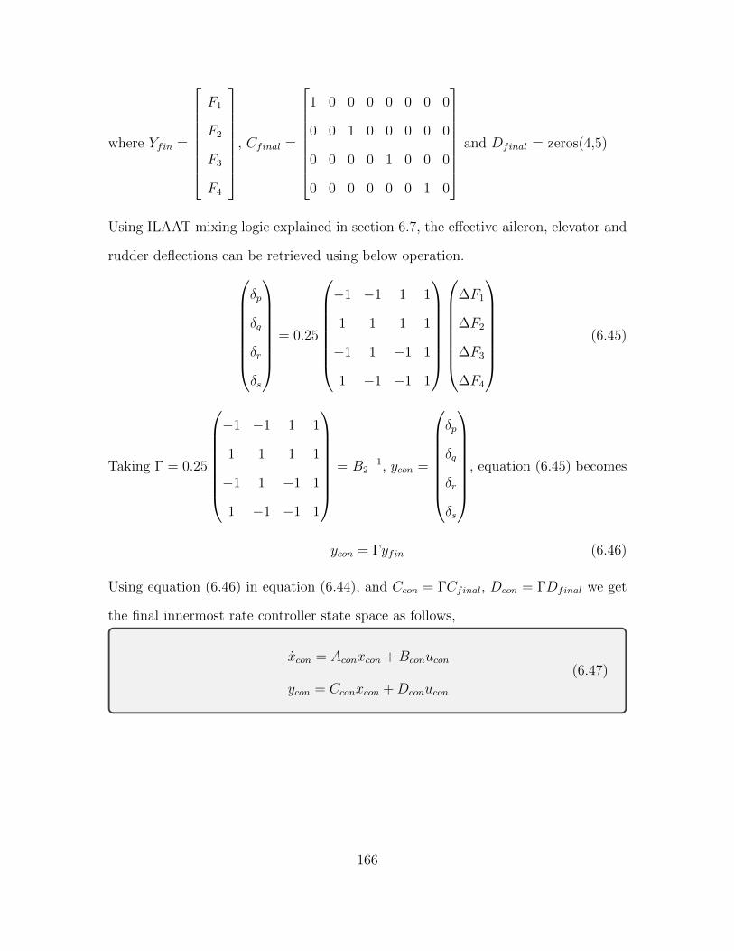
where Yfin =
F1
F2
F3
F4
, Cfinal =
1 0 0 0 0 0 0 0
0 0 1 0 0 0 0 0
0 0 0 0 1 0 0 0
0 0 0 0 0 0 1 0
and Dfinal = zeros(4,5)
Using ILAAT mixing logic explained in section 6.7, the effective aileron, elevator and
rudder deflections can be retrieved using below operation.
δp
δq
δr
δs
= 0.25
−1 −1 1 1
1 1 1 1
−1 1 −1 1
1 −1 −1 1
∆F1
∆F2
∆F3
∆F4
(6.45)
Taking Γ = 0.25
−1 −1 1 1
1 1 1 1
−1 1 −1 1
1 −1 −1 1
= B2
−1, ycon =
δp
δq
δr
δs
, equation (6.45) becomes
ycon = Γyfin (6.46)
Using equation (6.46) in equation (6.44), and Ccon = ΓCfinal, Dcon = ΓDfinal we get
the final innermost rate controller state space as follows,
xcon = Aconxcon +Bconucon
ycon = Cconxcon +Dconucon
(6.47)
166

6.9.3 Intermediate Loop
Figure 6.30: Block Diagram of Autopilot Intermediate Loop
Recalling the rate command generator equations which is the intermediate loop con-
troller in this case. The error in α & β signals have to be passed on to the innermost
loop.
Pc = K1(φc − φ)
Qc = K2(AzcL − Amz)
Qdp
− AzcLVb
Rc = K3(βc − β)
(6.48)
Rewriting above equation interms of error signals and taking K11 =(−K2 Sref CNα
Mass
),
defining error signals eφ = φc - φ, eα = αc - α and eβ = βc - β.
Pc = K1eφ
Qc = K11eα
Rc = K3eβ
(6.49)
Writing above equations in matrix form we get,
167
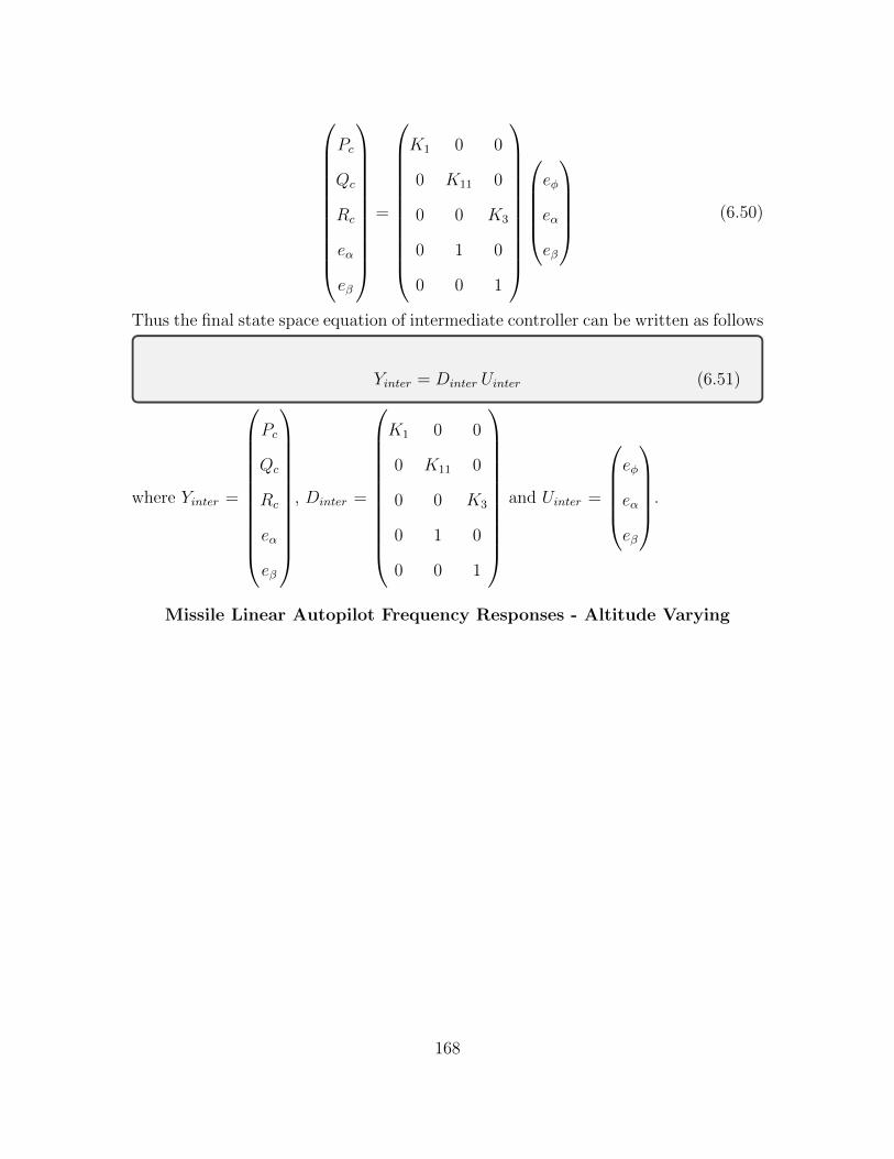
Pc
Qc
Rc
eα
eβ
=
K1 0 0
0 K11 0
0 0 K3
0 1 0
0 0 1
eφ
eα
eβ
(6.50)
Thus the final state space equation of intermediate controller can be written as follows
Yinter = Dinter Uinter (6.51)
where Yinter =
Pc
Qc
Rc
eα
eβ
, Dinter =
K1 0 0
0 K11 0
0 0 K3
0 1 0
0 0 1
and Uinter =
eφ
eα
eβ
.
Missile Linear Autopilot Frequency Responses - Altitude Varying
168

100
101
102
103
104−100
−90
−80
−70
−60
−50
−40
−30
−20
−10
0
Ki Frequency Response − Error
p to Aileron
Frequency (rad/sec)
Sin
gula
r V
alue
s (d
b)
Altitude = 40 kftAltitude = 50 kft
Figure 6.31: Ki − 1st Channel Frequency Response - Altitude Varying
101
102
103
−35
−30
−25
−20
−15
−10
−5
0
5
10
Ki Frequency Response − Error
q to Elevator
Frequency (rad/sec)
Sin
gula
r V
alue
s (d
b)
Altitude = 40 kftAltitude = 50 kft
Figure 6.32: Ki − 2nd Channel Frequency Response - Altitude Varying
169

100
101
102
103
104−70
−60
−50
−40
−30
−20
−10
0
10
Ki Frequency Response − Error
r to Rudder
Frequency (rad/sec)
Sin
gula
r V
alue
s (d
b)
Altitude = 40 kftAltitude = 50 kft
Figure 6.33: Ki − 3rd Channel Frequency Response - Altitude Varying
10−1
100
101
102
103−60
−50
−40
−30
−20
−10
0
Open Loop (PiK
i) Frequency Response − 1st Channel
Frequency (rad/sec)
Sin
gula
r V
alue
s (d
b)
Altitude = 40 kftAltitude = 50 kft
Figure 6.34: Open Loop Channel 1 Frequency Response - Altitude Varying
170

101
102
103−60
−50
−40
−30
−20
−10
0
10
20
Open Loop (PiK
i) Frequency Response − 2nd Channel
Frequency (rad/sec)
Sin
gula
r V
alue
s (d
b)
Altitude = 40 kftAltitude = 50 kft
Figure 6.35: Open Loop Channel 2 Frequency Response - Altitude Varying
10−2
10−1
100
101
102
103−80
−60
−40
−20
0
20
Open Loop (PiK
i) Frequency Response − 3rd Channel
Frequency (rad/sec)
Sin
gula
r V
alue
s (d
b)
Altitude = 40 kftAltitude = 50 kft
Figure 6.36: Open Loop Channel 3 Frequency Response - Altitude Varying
171

100
101
102
103−70
−60
−50
−40
−30
−20
−10
0
Inner Loop Pc to P − Sensitivities
Frequency (rad/sec)
Sin
gula
r V
alue
s (d
b)
T Alt = 40 kftS Alt = 40 kftT Alt = 50 kftS Alt = 50 kft
Figure 6.37: Inner Loop Complementary Sensitivity Pc vs P - Altitude Varying
101
102
103−60
−50
−40
−30
−20
−10
0
Inner Loop Qc to Q − Sensitivities
Frequency (rad/sec)
Sin
gula
r V
alue
s (d
b)
T Alt = 40 kftS Alt = 40 kftT Alt = 50 kftS Alt = 50 kft
Figure 6.38: Inner Loop Complementary Sensitivity Qc vs Q - Altitude Varying
172

101
102
103−80
−70
−60
−50
−40
−30
−20
−10
0
Inner Loop Rc to R − Sensitivities
Frequency (rad/sec)
Sin
gula
r V
alue
s (d
b)
T Alt = 40 kftS Alt = 40 kftT Alt = 50 kftS Alt = 50 kft
Figure 6.39: Inner Loop Complementary Sensitivity Rc vs R - Altitude Varying
10−1
100
101
102
103−40
−35
−30
−25
−20
−15
−10
−5
0
5Intermediate Loop φ Channel Sensitivities
Frequency (rad/sec)
Sin
gula
r V
alue
s (d
b)
T Alt = 40 kftS Alt = 40 kftT Alt = 50 kftS Alt = 50 kft
Figure 6.40: Intermediate Loop φ Channel Sensitivities - Altitude Varying
173

10−3
10−2
10−1
100
101
102−40
−35
−30
−25
−20
−15
−10
−5
0
5Intermediate Loop α Channel Sensitivities
Frequency (rad/sec)
Sin
gula
r V
alue
s (d
b)
T Alt = 40 kftS Alt = 40 kftT Alt = 50 kftS Alt = 50 kft
Figure 6.41: Intermediate Loop α Channel Sensitivities - Altitude Varying
10−2
10−1
100
101
102
103−40
−35
−30
−25
−20
−15
−10
−5
0
5Intermediate Loop β Channel Sensitivities
Frequency (rad/sec)
Sin
gula
r V
alue
s (d
b)
T Alt = 40 kftS Alt = 40 kftT Alt = 50 kftS Alt = 50 kft
Figure 6.42: Intermediate Loop β Channel Sensitivities - Altitude Varying
All the above figures, 6.31 - 6.42, exhibit the following behaviour and the reason
174

is explained below.
• As we go up, the air gets thinner.
• Missile fins can‘t operate efficiently at higher altitude because of the aerody-
namic properties there.
• Thus to pitch up or down, more than the elevator fin deflection, it is the angle
of attack that is more responsible for creating the required lift at such higher
altitudes.
• The missile system as a whole becomes smaller as RHP pole & RHP zero de-
crease in magnitude as altitude increases because of lower dynamic pressure.
Thus less bandwidth is required to to stabilize the missile. This the reason,
why BTT missiles (equivalent to passenger aircrafts) operate at cruise control
mode at higher altitude.
• Thus, it makes sense to have the autopilot to operate less aggressive as the
altitude increases.
• Figures 6.37-6.39 corresponding to innermost loop sensitivities and Figures 6.40-
6.42 corresponding to intermediate loop sensitivities show that their bandwidths
decrease (becomes less aggressive, i.e. sluggish) as altitude increases.
• Similar behaviour is exhibited by the controller and open loop (both pertaining
to innermost loop) frequency responses. The reader is referred to the figures
6.31 - 6.36 for observing the above said behaviour.
• It is very important to note here that, while the innermost rate control loop
operates at a bandwidth of about 10 radsec
(on all 3 channels), the intermediate
control loop operates at an bandwidth of about 1, 0.1 & 0.3 radsec
on φ, α &
175

β channels respectively which is about one decades slower than the innermost
loop. Innermost loop faster than the intermediate loop ensures that the overall
system is stable.
• α channel shows very less bandwidth, probably that is the reason why αc design
was omitted in the earlier designs as it does not bring in significant contribution
to the overall performance. Research was conducted which shows that missile
performance with the new αc design and without it (old) design, showed no
significant improvements. The new αc was included because it is very important
from a BTT missile point of view as BTT missile maneuvers by banking to
desired orientation first and then angle of attack is varied in that normal plane
to achieve the desired orientation while stabilizing the roll missile. The author
feels this should need more investigation as to why this behaviour is exhibited.
Missile Linear Autopilot Frequency Responses - Mach Varying
101
102
103−40
−35
−30
−25
−20
−15
−10
−5
0
Ki Frequency Response − Error
p to Aileron
Frequency (rad/sec)
Sin
gula
r V
alue
s (d
b)
Mach = 1.068Mach = 1.5114
Figure 6.43: Ki − 1st Channel Frequency Response - Mach Varying
176

101
102
103−20
−15
−10
−5
0
5
10
15
20
Ki Frequency Response − Error
q to Elevator
Frequency (rad/sec)
Sin
gula
r V
alue
s (d
b)
Mach = 1.068Mach = 1.5114
Figure 6.44: Ki − 2nd Channel Frequency Response - Mach Varying
101
102
103−25
−20
−15
−10
−5
0
5
10
15
20
Ki Frequency Response − Error
r to Rudder
Frequency (rad/sec)
Sin
gula
r V
alue
s (d
b)
Mach = 1.068Mach = 1.5114
Figure 6.45: Ki − 3rd Channel Frequency Response - Mach Varying
177

101
102
103−50
−40
−30
−20
−10
0
10
20
Open Loop (PiK
i) Frequency Response − 1st Channel
Frequency (rad/sec)
Sin
gula
r V
alue
s (d
b)
Mach = 1.068Mach = 1.5114
Figure 6.46: Open Loop Channel 1 Frequency Response - Mach Varying
101
102
103−50
−40
−30
−20
−10
0
10
20
Open Loop (PiK
i) Frequency Response − 2nd Channel
Frequency (rad/sec)
Sin
gula
r V
alue
s (d
b)
Mach = 1.068Mach = 1.5114
Figure 6.47: Open Loop Channel 2 Frequency Response - Mach Varying
178

10−1
100
101
102
103−50
−40
−30
−20
−10
0
10
20
30
40
Open Loop (PiK
i) Frequency Response − 3rd Channel
Frequency (rad/sec)
Sin
gula
r V
alue
s (d
b)
Mach = 1.068Mach = 1.5114
Figure 6.48: Open Loop Channel 3 Frequency Response - Mach Varying
100
101
102
103−50
−40
−30
−20
−10
0
10
20
Inner Loop P channel Sensitivities
Frequency (rad/sec)
Sin
gula
r V
alue
s (d
b)
T Mach = 1.068S Mach = 1.068T Mach = 1.5114S Mach = 1.5114
Figure 6.49: Inner Loop Complementary Sensitivity Pc vs P - Mach Varying
179

101
102
103−50
−40
−30
−20
−10
0
10
20
Inner Loop Q channel Sensitivities
Frequency (rad/sec)
Sin
gula
r V
alue
s (d
b)
T Mach = 1.068S Mach = 1.068T Mach = 1.5114S Mach = 1.5114
Figure 6.50: Inner Loop Complementary Sensitivity Qc vs Q - Mach Varying
100
101
102
103−50
−40
−30
−20
−10
0
10
20Inner Loop R channel Sensitivities
Frequency (rad/sec)
Sin
gula
r V
alue
s (d
b)
T Mach = 1.068S Mach = 1.068T Mach = 1.5114S Mach = 1.5114
Figure 6.51: Inner Loop Complementary Sensitivity Rc vs R - Mach Varying
180
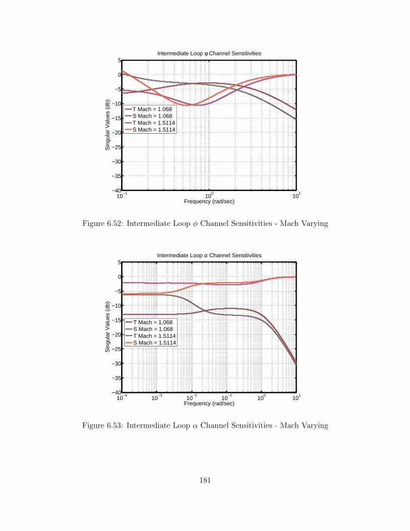
10−1
100
101−40
−35
−30
−25
−20
−15
−10
−5
0
5Intermediate Loop φ Channel Sensitivities
Frequency (rad/sec)
Sin
gula
r V
alue
s (d
b)
T Mach = 1.068S Mach = 1.068T Mach = 1.5114S Mach = 1.5114
Figure 6.52: Intermediate Loop φ Channel Sensitivities - Mach Varying
10−4
10−3
10−2
10−1
100
101−40
−35
−30
−25
−20
−15
−10
−5
0
5Intermediate Loop α Channel Sensitivities
Frequency (rad/sec)
Sin
gula
r V
alue
s (d
b)
T Mach = 1.068S Mach = 1.068T Mach = 1.5114S Mach = 1.5114
Figure 6.53: Intermediate Loop α Channel Sensitivities - Mach Varying
181

10−1
100
101−30
−25
−20
−15
−10
−5
0
5Intermediate Loop β Channel Sensitivities
Frequency (rad/sec)
Sin
gula
r V
alue
s (d
b)
T Mach = 1.068S Mach = 1.068T Mach = 1.5114S Mach = 1.5114
Figure 6.54: Intermediate Loop β Channel Sensitivities - Mach Varying
All the above figures, 6.43 - 6.54, exhibit the following behaviour and the reason
is explained below.
• We know from figure 3.47, that Mach ∝ 1h.
• The missile system as a whole becomes bigger as RHP pole & RHP zero increase
in magnitude as Mach increases because of higher dynamic pressure. Thus more
bandwidth is required to to stabilize the missile.
• Thus, it makes sense to have the autopilot to operate more aggressive as the
Mach increases, mainly because the unstable pole grows in magnitude.
• Figures 6.49-6.51 corresponding to innermost loop sensitivities and Figures 6.52-
6.54 corresponding to intermediate loop sensitivities corresponding to the longi-
tudinal variables show that their bandwidths increase (becomes more aggressive,
i.e. faster) as Mach increases.
182

• Similar behaviour is exhibited by the controller and open loop (both pertaining
to innermost loop) frequency responses corresponding to the longitudinal vari-
ables. The reader is referred to the figures 6.43 - 6.48 for observing the above
said behaviour.
• It is very important to note here that, while the innermost rate control loop
operates at a bandwidth of about 10 radsec
(on all 3 channels), the intermediate
control loop operates at an bandwidth of about 0.5, 0.01 & 0.5 radsec
on φ, α
& β channels respectively which is about roughly one decades slower than the
innermost loop. Innermost loop faster than the intermediate loop ensures that
the overall system is stable.
6.10 Summary and Conclusions
This chapter has provided a comprehensive case study for our BTT Missile Au-
topilot. After the brief explanation of control law formulation using Incremental
Nonlinear Dynamic Inversion technique, the nonlinear autopilot was explained, fol-
lowed by its linearization and its analysis. The analysis show that the autopilot is
very robust and properly follows the signal commands issued.
183

Chapter 7
NUMERICAL INTEGRATION
7.1 Introduction and Overview
Within this chapter, we address obtaining approximate solutions for the differ-
ential equations governing missile dynamics using numerical integration methods.
Differential equations of first order can be solved using variety of mathematical tools.
But for solving the equations using different initial conditions and real time inputs, we
need a computer generated approximate solution. This is where numerical integration
techniques, in particular Runge-Kutta methods come handy. Motivational examples
from [68] are examined. Expecting a miss distance within the blast radius of the
missile [70], nominal step size selection for a desired level of accuracy is demonstrated
using missile target engagement geometry simulations.
Choosing an ideal step size for simulation is really important. Smaller the step
size, more frequent the decisions are made about the next move. Given a small step
size, missile moves a very small distance between each step towards the target. Sim-
ilarly the larger step size involves less frequent decision making and missile moves
to a big distance between each step towards the target. Going by the intuition, we
normally prefer a smaller step size as we need a higher level of accuracy. Accuracy
in this context refers to the final miss distance between missile and target. Conven-
tional medium range missiles carrying high explosive warhead have blast radius of
about 20ft [70]. This gives us an excellent information about what final miss distance
we are looking for from our simulation. Smaller step size enjoys another benefit of
184

not loading the actuators to perform till their saturation level continuously. This is
evident from both the fin actuator and fin rate responses provided in this chapter.
To avoid making baby steps towards the target, we try to increase the step size
and see where it starts to behave bad. The highest value of step size that gives us
minimum miss distance without loading the actuators much is the ideal one. Trying
an higher step size might even make a missile to miss the target initially and try hard
enough to intercept it later. Given this, during such an awkward situation caused by
larger step size, the autopilot is forced to make the actuators to work in the saturated
level contantly. Thus engagement geometry of the missile target engagement is not
smooth, making the life of the missile hard. The key goal of this chapter is to explain
about the trade off involved in selection of ideal step size for integration.
Remainder of this chapter is organized as follows: In Section 7.2 all four Runge-
Kutta methods are explained with an example and results are tabulated. Then step
size selection through engagement geometry is explained in Section 7.3. Finally Sec-
tion 7.4 summarizes and concludes the work explained in this chapter.
7.2 Runge-Kutta(RK) Integration Methods
Lets consider an initial value problem,
f(t, y) =dy
dt= y − t2 + 1 (7.1)
where t0 = 0 and y(t0) =y0 = 0.5 are the initial conditions considered. We need to
solve for y between 0 ≤ t ≤ 2. Let “h” be the step size. Analytically solving this
problem we get,
y(t) = t2 + 2t+ 1− et
2(7.2)
185

y(t=2) = 5.305471950534675 as the exact solution. In normal integration with end-
points, we just use the end points of interval, and we dont know how the system
behaves in between. Here, integration is carried out in small step size, which cap-
tures the behavior of system exactly over the entire time interval. This inherently
tells us to keep the step size as minimum as possible to get a better solution. But
decreasing the step size will increase the computational effort. Thus, a trade-off has
to be observed between the two in order to get a desired level of accurate solution.
Depending upon the importance given to the slope of function at different points in
the interval, there are different types of methods available. Methods discussed below
are Runge Kutta - 1st, 2nd, 4th&Fehlberg.
7.2.1 Runge-Kutta 1st Method
Also called as the Eulers method of integration, solution is given by equation 7.3
given below,
y(t+ h) = y(t) + hdy(t, y)
dt(7.3)
The next value is found out using value of function at that instant of time and deriva-
tive at that instant of time. The error between actual solution and approximated
solution at all instances is relatively high in this method. Solving above example
problem with this method we get 5.3001 as the final solution. Also, the error value is
5.3055 - 5.3001 = 0.0054. This is a high value of error given the accuracy of computers
today. So this approximation is acceptable to certain extent.
7.2.2 Runge-Kutta 2nd Method
Demanding need for more accuracy, we go for 2nd method, where slope at mid-
point of the interval is considered for better approximation. The solution is given by
186

equation 7.4 given below,
y(t+ h) = y(t) + k2
k1 = hdy(t, y)
dt
k2 = hdy(t+ 0.5h, y + k1)
dt
(7.4)
Solving above example problem with this method, we get w = 5.3196 as the final
solution. The error value between approximate solution and true sollution is still
high. So this approximation is also acceptable only to a certain extent.
7.2.3 Runge-Kutta 4th Method
This is also called classical Runge-Kutta method. This takes into account the slope
of function at beginning, at the midpoint and at the end of interval to approximate
the solution. Taking “h” to be the step size such that ti = t0 + ih, the solution is
given by equation 7.5 given below,
wi ≈ y(ti), where
wi+1 = wi +1
6(k1 + 2k2 + 2k3 + k4)
k1 = hf(ti, wi)
k2 = hf
(ti +
h
2, wi +
k1
2
)k3 = hf
(ti +
h
2, wi +
k2
2
)k4 = hf(ti + h,wi + k3)
(7.5)
Solving above example problem with this method, we get 5.3055 as the final
solution, error value between approximated solution and exact solution is negligible.
We now know that this method is very good, only drawback being going through
same step size for each and every iteration before settling down.
187

7.2.4 Adaptive Step Size - Runge-Kutta-Fehlberg Method
The error is compared with a threshold value at every step. If it is less than(more
than) the threshold, we increase(decrease) the step size and re-do the current step
again. This way, instead of going through same step size throughout the interval, we
move forward intelligently adapting the step size. The solution is given by equation
7.6 given below,
R =1
h|wi+1 − wi+1|
wi+1 = wi +25
216k1 +
1408
2565k3 +
2197
4104k4 −
1
5k5
wi+1 = wi +16
135k1 +
6656
12825k3 +
28561
56430k4 −
9
50k5 +
2
55k6
k1 = hf(ti, wi)
k2 = hf
(ti +
h
4, wi +
k1
4
)k3 = hf
(ti +
3h
8, wi +
3
32k1 +
9
32k2
)k4 = hf
(ti +
12h
13, wi +
1932
2197k1 +
7200
2197k2 +
7296
2197k3
)k5 = hf
(ti + h,wi +
439
216k1 − 8k2 +
3680
513k3 +
845
4104k4
)k6 = hf
(ti +
h
2, wi −
8
27k1 + k1 + 2k2 −
3544
2565k3 +
1859
4104k4 −
11
40k5
)δ = 0.84
( εR
) 14
(7.6)
if R ≤ ε Keep w as the current step
solution and move to the
next step with the step size
δh
if R > ε recalculate the current step
with the step size δh
188

Solving above example problem with this method, we get 5.3055 as the final
solution, which was obtained in very less amount of steps. The error is as usual very
negligible like RK-4 method since internally this method used RK4 for approximation.
Integration
Method
Error between True
and Approximate
Solutions
Computational
Effort
No. of Itera-
tions
RK-1 High Very Less More
RK-2 Considerably Low Less More
RK-4 Very Negligible High More
RK-Fehlberg Very negligible Very high Very Less
Table 7.1: Comparison of Runge-Kutta Integration Methods
7.3 Nominal Step Size Selection using Engagement Geometry Analysis
Optimal step size will enable a smooth flight for missile without loading the ac-
tuators heavily and it will enable the missile to intercept the target with excellent
accuracy. Here in this research, the target maneuvered using the sheldon mode while
the missile tried intercepting it using optimal guidance and for the same initial flight
conditions given by Table 7.2, the step size was varied to see where the simulation
started to fail. This will give us an upper bound on the step size. See Figure 7.1.
Similarly even smaller step sizes were tried and they gave us satisfactory results. See
Figure 7.2. But they were having longer flight time because the missile was making
baby steps towards the target. So to fasten the decision process and that too with
expected accuracy, the optimal step size was selected which resulted in both fast and
accurate simulations.
189

Flight Parameter Value Flight Parameter Value
Missile Max. Accel. 80 g Initial Height -1000 ft
Initial Missile Mach 0.8999 Target Range 2000 ft
Initial Target Mach 0.8999 Time Constant 0.5 sec
Azimuth Angle 0 deg Aspect Angle 0 deg
Table 7.2: Flight Conditions for Miss Distance vs Integration Step Size
0.002 0.004 0.006 0.008 0.01 0.012 0.014 0.016 0.018 0.02
20
40
60
80
100
120
Miss Distance vs Step Size
X: 0.001Y: 4.968
step time (sec)
mis
s di
stan
ce (
ft)
X: 0.0005Y: 4.926
X: 0.005Y: 5.863
Figure 7.1: Miss Distance vs Integration Step Size
190

0.5 1 1.5 2 2.5 3 3.5
x 10−3
6
8
10
12
14
16
18
X: 0.001Y: 4.968
step time (sec)
mis
s di
stan
ce (
ft)
X: 0.0005Y: 4.926
Figure 7.2: Zoomed in Figure 7.1
Engagement Geometry. Referring to Figures 7.3 and 7.5, it is evident that smaller
step sizes gave a smooth engagement geometry, while larger step sizes made the life
of missile difficult. By careful observation of Figures 7.3 and 7.4, it can be easily seen
that as the step size grows larger, the missile starts to miss the target resulting in
a bad simulation. It is important to emphasize here that a bad step size will result
only in a bad simulation resulting in the missile missing the target, while it does not
imply that the missile does not have the capability to hit the target. While operated
with a big step size, the missile tries to the best of its abilities to make sharp turns
to intercept the target even if it misses the target at initial ranges. While doing
sharp turns, the missile fin actuators hit their saturation levels frequently, which is
obviously not a good condition for fin actuators. The reader is referred to the Figures
7.7 and 7.8 to visualize the phenomenon explained above.
191

0
500
1000
1500
2000
0 100 200 300 400 500 600 700
950
1000
1050
X (ft)
Missile/Target Trajectory vs Step Time
Y (ft)
Z (
ft)missile
0.005
missile0.008
missile0.010
missile0.015
missile0.018
missile0.019
missile0.020
target
Figure 7.3: Engagement Geometry 3D Plot for different step sizes
0200400600800100012001400160018002000
0
100
200
300
400
500
600
700
X (ft)
Missile/Target Trajectory vs Step Time
Y (
ft)
missile0.005
missile0.008
missile0.010
missile0.015
missile0.018
missile0.019
missile0.020
target
Figure 7.4: Engagement Geometry 2D Plot for different step sizes
192
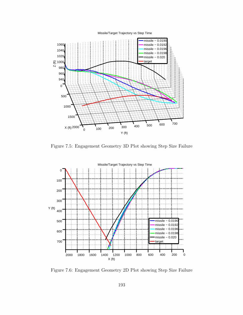
0
500
1000
1500
20000 100 200 300 400 500 600 700
940
960
980
1000
1020
1040
1060
Missile/Target Trajectory vs Step Time
Y (ft)
X (ft)
Z (
ft)
missile − 0.0190missile − 0.0192missile − 0.0196missile − 0.0198missile − 0.020target
Figure 7.5: Engagement Geometry 3D Plot showing Step Size Failure
0200400600800100012001400160018002000
0
100
200
300
400
500
600
700
Missile/Target Trajectory vs Step Time
X (ft)
Y (ft)
missile − 0.0190missile − 0.0192missile − 0.0196missile − 0.0198missile − 0.020target
Figure 7.6: Engagement Geometry 2D Plot showing Step Size Failure
193

0 0.1 0.2 0.3 0.4 0.5 0.6 0.7 0.8 0.9 1−600
−400
−200
0
200
400
Fin 1 Rate vs Flight Time for Step time = 0.0005 sec
Flight Time (sec)
Fin
1 R
ate
(deg
/sec
)
Figure 7.7: Fin Deflection Rate for Smaller Step Size
0 0.1 0.2 0.3 0.4 0.5 0.6 0.7 0.8 0.9 1−600
−400
−200
0
200
400
600Fin 1 Rate vs Flight Time for Step time = 0.0195 sec
Flight Time (sec)
Fin
1 R
ate
(deg
/sec
)
Figure 7.8: Fin Deflection Rate for Bigger Step Size
194

For the above initial flight conditions, step size of 0.005 would be very optimal which
can be seen through the Figure 7.1. This optimal step size is expected to vary for
different range and other flight conditions.
7.4 Summary and Conclusions
This chapter gives a brief idea about the proper usage of numerical integration in
complex simulation like missile guidance control systems. The four different Runge-
Kutta methods were explained using a mathematical example and their merits and
demerits were tabulated. Then the procedure to select the optimal step size for numer-
ical integration was explained using the engagement geometry analysis. Effect of bad
step size selection on actuators hitting their saturation levels were clearly explained.
Thus the purpose of the chapter was to provide a solid foundation on the numerical
integration methods used to numerically approximate the complex, nonlinear missile
and target differential equations during the missile target engagement.
195

Chapter 8
MISS DISTANCE ANALYSIS
8.1 Introduction and Overview
The purpose of this chapter is to illustrate the hunting capabilities of the BTT
missile considered in this research. Given a thrust profile and fixed initial conditions,
the analysis made in this chapter will answer how good a missile will be in intercepting
a target within its killing range. The high fidelity environment used throughout the
simulation used in this research is employed to study the miss distance profile with
respect to different missile/target engagement parameters as described in the relevant
GNC textbooks [51] and [52]. Also the work done in this chapter will lay a basic
foundation and serve as a perfect motivation factor for kill zone estimation, which
is explained in brief in the Chapter 9. Conventional warheads carried by the missile
have a circular blast radius of about 20 ft [70]. Thus any simulation resulting in a
final miss distance less than 20 feet is taken granted as a hit and miss distance profile
is obtained as per this logic. Each section in this chapter will have information about
the flight conditions considered, the result and its inference. The chapter is organized
as follows: Section 8.2 will briefly discuss the miss distance profile change when
the proportional gain is varied. Here the missile is assumed to possess Proportional
Navigation guidance law to intercept the target. Section 8.3 analyses the effect of
altitude variation on the miss distance profile. Section 8.4 throws light on effect
of varying the maximum acceleration capability of the missile over the final miss
distance achieved. Section 8.5 discusses the effect of initial missile speed on the final
miss distance profile. Section 8.6 establishes a brief idea about how the miss distance
196

profile varies as the target is made to maneuver more and more. Missile is assumed
to possess Differential Game Theory guidance to intercept the target here. Section
8.7 shows how the miss distance varies when the target’s orientation with respect
to the missile measured in terms of Aspect. Section 8.8 elaborates how the miss
distance varies when the initial range is varied. This motivates the work done in the
entire Chapter 9. Finally Section 8.9 summarizes and concludes the work done in
this chapter and gives a rough idea about estimating the missile’s capabilities using
above analyses.
8.2 Miss Distance Dependence on Proportional Gain
Throughout the simulation conducted here in this section, the missile is made
to possess proportional navigation guidance and all the three target maneuvers are
tested by varying the proportional gain. The initial flight conditions considered are
shown in the Table 8.1.
Flight Conditions Considered:
Flight Parameter Value Flight Parameter Value
Missile Max. Accel. 80 g Initial Height -1000 ft
Initial Missile Mach 0.8999 Target Range 2000 ft
Initial Target Mach 0.8999 Integration Method RK-4
Guidance Law Proportional Aspect Angle 135 deg
Table 8.1: Flight Conditions for Miss Distance vs Proportional Gain
197

−1 0 1 2 3 4 5 6 7 8 90
50
100
150
200
250
300
350
400
450
500
Proportional Navigation Gain
Mis
s D
ista
nce
(ft)
Miss Distance vs Proportional Navigation Gain
No AccelerationSheldon Turn & ClimbRiggs Vergaz Turn & Dive
Figure 8.1: Miss Distance vs Proportional Gain
2 3 4 5 6 7 80
5
10
15
20
25
30
35
40
45
Proportional Navigation Gain
Mis
s D
ista
nce
(ft)
Miss Distance vs Proportional Navigation Gain
No AccelerationSheldon Turn & ClimbRiggs Vergaz Turn & Dive
Figure 8.2: Zoomed in Figure 8.1
Inferences.
• From Figures 8.1 and 8.2, it is clearly evident that the miss distance is higher
198

when the proportional gain is too small and the miss distance reaches the min-
imum value which is unique for different flight conditions.
• Beyond the minimum, the miss distance increases slowly as we increase the gain
and this behaviour persists irrespective of the target maneuver.
• It is intuitive that if the proportional gain is very small, the missile will respond
slowly and will not be able to catch the target and similarly if the gain is big,
the outer guidance loop will become unstable due to the high frequency seeker
dynamics.
• It is also observed that these changes are observed only when the initial altitude
is small. At higher altitudes, the miss distance essentially becomes independent
of the gain.
• The reader is referred to the [17] for further insight and information about this
section.
8.3 Miss Distance Dependence on Initial Engagement Altitude
Throughout the simulation conducted here in this section, the missile is made
to possess different guidance laws and all the three target maneuvers are tested by
varying the initial engagement altitude. The initial flight conditions considered are
shown in the Table 8.2.
Flight Conditions Considered:
199

Flight Parameter Value Flight Parameter Value
Missile Max. Accel. 80 g Maneuver Index 0.25
Initial Missile Mach 0.8999 Target Range 2000 ft
Initial Target Mach 0.8999 Intgration Method RK-4
Proportional Gain 2.1 Aspect Angle 135 deg
Table 8.2: Flight Conditions for Miss Distance vs Engagement Altitude
0 10 20 30 40 50 60 70 800
50
100
150
200
250
300
350
400
450
500
Altitude (kft)
Mis
s D
ista
nce
(ft)
Miss Distance vs Altitude (No Maneuver)
Proportional NavigationOptimal TheoryDifferential Game Theory
Figure 8.3: Miss Distance vs Engagement Altitude - No Maneuver
200

0 10 20 30 40 50 60 70 800
50
100
150
200
250
300
350
400
450
500
Altitude (kft)
Mis
s D
ista
nce
(ft)
Miss Distance vs Altitude (Sheldon Maneuver)
Proportional NavigationOptimal TheoryDifferential Game Theory
Figure 8.4: Miss Distance vs Engagement Altitude - Sheldon Maneuver
0 10 20 30 40 50 60 70 800
50
100
150
200
250
300
350
400
450
500
Altitude (kft)
Mis
s D
ista
nce
(ft)
Miss Distance vs Altitude (Riggs Vergaz Maneuver)
Proportional NavigationOptimal TheoryDifferential Game Theory
Figure 8.5: Miss Distance vs Engagement Altitude - Riggs Vergaz Maneuver
201
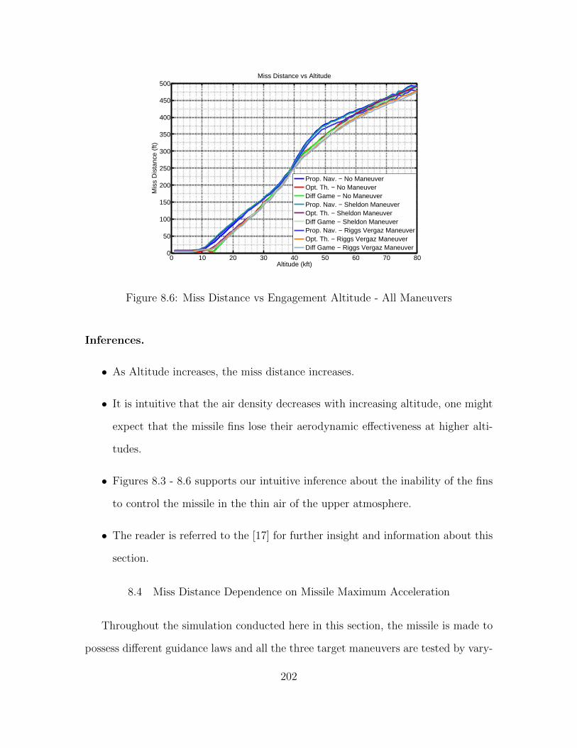
0 10 20 30 40 50 60 70 800
50
100
150
200
250
300
350
400
450
500
Altitude (kft)
Mis
s D
ista
nce
(ft)
Miss Distance vs Altitude
Prop. Nav. − No ManeuverOpt. Th. − No ManeuverDiff Game − No ManeuverProp. Nav. − Sheldon ManeuverOpt. Th. − Sheldon ManeuverDiff Game − Sheldon ManeuverProp. Nav. − Riggs Vergaz ManeuverOpt. Th. − Riggs Vergaz ManeuverDiff Game − Riggs Vergaz Maneuver
Figure 8.6: Miss Distance vs Engagement Altitude - All Maneuvers
Inferences.
• As Altitude increases, the miss distance increases.
• It is intuitive that the air density decreases with increasing altitude, one might
expect that the missile fins lose their aerodynamic effectiveness at higher alti-
tudes.
• Figures 8.3 - 8.6 supports our intuitive inference about the inability of the fins
to control the missile in the thin air of the upper atmosphere.
• The reader is referred to the [17] for further insight and information about this
section.
8.4 Miss Distance Dependence on Missile Maximum Acceleration
Throughout the simulation conducted here in this section, the missile is made to
possess different guidance laws and all the three target maneuvers are tested by vary-
202

ing the initial maximum missile acceleration. The initial flight conditions considered
are shown in the Table 8.3.
Flight Conditions Considered:
Flight Parameter Value Flight Parameter Value
Proportional Gain 2.1 Maneuver Index 0.25
Initial Missile Mach 0.8999 Target Range 2000 ft
Initial Target Mach 0.8999 Time Constant 0.5 sec
Altitude -1000 ft Aspect Angle 135 deg
Table 8.3: Flight Conditions for Miss Distance vs Missile Maximum Acceleration
10 20 30 40 50 60 70 800
100
200
300
400
500
600
Missile Maximum Acceleration (g)
Mis
s D
ista
nce
(ft)
Miss Distance vs Missile Maximum Acceleration (No Maneuver)
Proportional NavigationOptimal Control TheoryDifferential Game Theory
Figure 8.7: Miss Distance vs Missile Max. Acceleration - No Maneuver
203
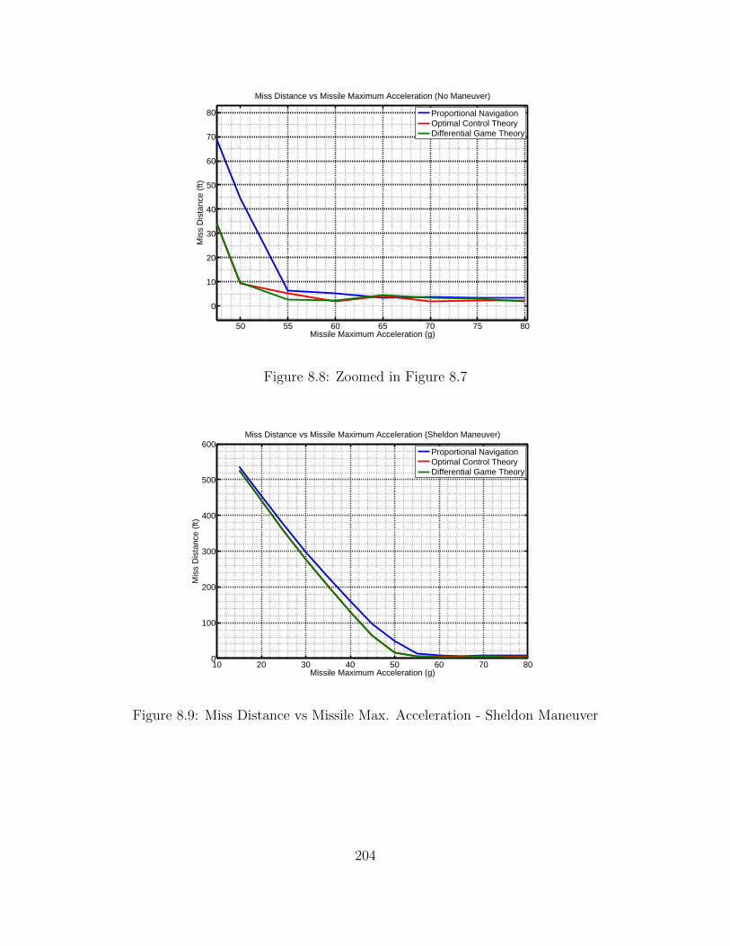
50 55 60 65 70 75 80
0
10
20
30
40
50
60
70
80
Missile Maximum Acceleration (g)
Mis
s D
ista
nce
(ft)
Miss Distance vs Missile Maximum Acceleration (No Maneuver)
Proportional NavigationOptimal Control TheoryDifferential Game Theory
Figure 8.8: Zoomed in Figure 8.7
10 20 30 40 50 60 70 800
100
200
300
400
500
600
Missile Maximum Acceleration (g)
Mis
s D
ista
nce
(ft)
Miss Distance vs Missile Maximum Acceleration (Sheldon Maneuver)
Proportional NavigationOptimal Control TheoryDifferential Game Theory
Figure 8.9: Miss Distance vs Missile Max. Acceleration - Sheldon Maneuver
204

50 55 60 65 70 75 800
10
20
30
40
50
60
70
80
Missile Maximum Acceleration (g)
Mis
s D
ista
nce
(ft)
Miss Distance vs Missile Maximum Acceleration (Sheldon Maneuver)
Proportional NavigationOptimal Control TheoryDifferential Game Theory
Figure 8.10: Zoomed in Figure 8.9
10 20 30 40 50 60 70 800
100
200
300
400
500
600
Missile Maximum Acceleration (g)
Mis
s D
ista
nce
(ft)
Miss Distance vs Missile Maximum Acceleration (Riggs Vergaz Maneuver)
Proportional NavigationOptimal Control TheoryDifferential Game Theory
Figure 8.11: Miss Distance vs Missile Max. Acceleration - Riggs Vergaz Maneuver
205

50 55 60 65 70 75 800
10
20
30
40
50
60
70
80
Missile Maximum Acceleration (g)
Mis
s D
ista
nce
(ft)
Miss Distance vs Missile Maximum Acceleration (Riggs Vergaz Maneuver)
Proportional NavigationOptimal Control TheoryDifferential Game Theory
Figure 8.12: Zoomed in Figure 8.11
10 20 30 40 50 60 70 800
50
100
150
200
250
300
350
Missile Maximum Acceleration (g)
Mis
s D
ista
nce
(ft)
Miss Distance vs Missile Maximum Acceleration
Prop. Nav. − No ManeuverOpt. Th. − No ManeuverDiff Game − No ManeuverProp. Nav. − Sheldon ManeuverOpt. Th. − Sheldon ManeuverDiff Game − Sheldon ManeuverProp. Nav. − Riggs Vergaz ManeuverOpt. Th. − Riggs Vergaz ManeuverDiff Game − Riggs Vergaz Maneuver
Figure 8.13: Miss Distance vs Missile Max. Acceleration - All Maneuvers
206

50 55 60 65 70 75 800
10
20
30
40
50
60
Missile Maximum Acceleration (g)
Mis
s D
ista
nce
(ft)
Miss Distance vs Missile Maximum Acceleration
Prop. Nav. − No ManeuverOpt. Th. − No ManeuverDiff Game − No ManeuverProp. Nav. − Sheldon ManeuverOpt. Th. − Sheldon ManeuverDiff Game − Sheldon ManeuverProp. Nav. − Riggs Vergaz ManeuverOpt. Th. − Riggs Vergaz ManeuverDiff Game − Riggs Vergaz Maneuver
Figure 8.14: Zoomed in Figure 8.13
Inferences.
• As missile maximum acceleration increases, the miss distance decreases.
• This goes well with our intuition that given an higher acceleration advantage for
the missile over the target, it is easier for the missile to track down the target.
• Figures 8.7 - 8.14 support our inferences.
• It is also seen that irrespective of the different target maneuver and different
missile guidance laws, the above said conjecture seems to hold true.
8.5 Miss Distance Dependence on Initial Missile Mach
Throughout the simulation conducted here in this section, the missile is made to
possess proportional guidance law and the target has no maneuver and this scenario
is tested by varying the initial missile Mach. The initial flight conditions considered
are shown in the Table 8.4.
207

Flight Conditions Considered:
Flight Parameter Value Flight Parameter Value
Missile Max. Accel. 80 g Initial Height -1000 ft
Integration Method RK-4 Target Range 10000 ft
Initial Target Mach 0.8999 Time Constant 0.5 sec
Target Mode Const. Ve-
locity
Aspect Angle 135 deg
Table 8.4: Flight Conditions for Miss Distance vs Missile Mach
0.8 1 1.2 1.4 1.6 1.8 2 2.20
50
100
150
200
250
300
350
400
Mach
Mis
s D
ista
nce
(ft)
Miss Distance vs Missile Mach
Figure 8.15: Miss Distance vs Initial Missile Mach
Inferences.
• It is intuitive that the missile will track its target if it is given an higher initial
velocity.
208

• But it is also a point of interest to note here that, if the missile initial velocity
is very big, e.g. here in our case if it is bigger than 2.15 for the above flight
condition considered, the missile permanenetly misses the target because it had
travelled probably in the wrong direction initially with higher velocity.
• Missile realizes that the it cannot track down its target as the range keeps on
increasing.
• That is not captured here in Figure 8.15 as miss distance is a very big number
in those cases.
• This scenario can be thought analogous to a condition where our integration
step size is big.
• Reader is referred to the Section 7.3 in Chapter 7.
8.6 Miss Distance Dependence on Target Maneuver
Throughout the simulation conducted here in this section, the missile is made
to possess differential game theory guidance and all the three target maneuvers are
tested by varying the proportional gain. The initial flight conditions considered are
shown in the Table 8.5.
Flight Conditions Considered:
209

Flight Parameter Value Flight Parameter Value
Missile Max. Accel. 80 g Initial Height -1000 ft
Initial Missile Mach 0.8999 Target Range 2000 ft
Initial Target Mach 0.8999 Time Constant 0.5 sec
Integration Method RK-4 Aspect Angle 135 deg
Table 8.5: Flight Conditions for Miss Distance vs Target Maneuver
0 0.5 1 1.5 2 2.5 3 3.50
50
100
150
200
250
300
350
Target Maneuver Index
Mis
s D
ista
nce
(ft)
Miss Distance vs Target Maneuver Index
No AccelerationSheldon Turn & ClimbRiggs Vergaz Turn & Dive
Figure 8.16: Miss Distance vs Target Maneuver
210

0.1 0.2 0.3 0.4 0.5 0.6 0.7 0.8 0.9
0
5
10
15
20
Target Maneuver Index
Mis
s D
ista
nce
(ft)
Miss Distance vs Target Maneuver Index
No AccelerationSheldon Turn & ClimbRiggs Vergaz Turn & Dive
Figure 8.17: Zoomed in Figure 8.16
Inferences.
• From Figure 8.16 & 8.17, it is clear that as the target maneuvers more, it is
difficult for the missile to intercept it.
• The degree of target maneuverability is measured using an unitless quantity
called “Target Maneuver Index” or simply “Maneuver Index(MI)”. We know
that from equation 4.37.
• It is clear that as long as Maneuver Index is small, the differential game thoery
guidance is going to behave well as smaller MI indicates target maneuvering
very less.
• But as MI approaches 1, its singular point, the miss distance starts to increase.
• Thus, for all values of MI > 1, which indicates the target maneuvering more,
the miss distance is bad (i.e. the missile misses the target) irrespective of the
target’s intelligence.
211

• This behaviour is excellently captured in the Figure 8.16.
• For more information on this concept, the reader is referred to the relevant GNC
texts [51] and [52].
8.7 Miss Distance Dependence on Target Aspect
Throughout the simulation conducted here in this section, the missile is made to
possess proportional guidance and the target doesn’t maneuver. This flight condition
is tested by varying the initial target aspect with respect to the missile. The initial
flight conditions considered are shown in the Table 8.6.
Flight Conditions Considered:
Flight Parameter Value Flight Parameter Value
Missile Max. Accel. 80 g Initial Height -1000 ft
Initial Missile Mach 0.8999 Target Range 1-10 kft
Initial Target Mach 0.8999 Time Constant 0.5 sec
Target Mode Const. Ve-
locity
Integration Method RK-4
Table 8.6: Flight Conditions for Miss Distance vs Target Aspect
212

0 20 40 60 80 100 120 140 160 1800
500
1000
1500
2000
2500
3000
3500
4000
4500
Aspect Angle (deg)
Mis
s D
ista
nce
(ft)
Miss Distance vs Aspect Angle
Range = 1000 ftRange = 2000 ft
Figure 8.18: Miss Distance vs Target Aspect - Range = 1 kft, 2 kft
20 40 60 80 100 120
−5
0
5
10
Aspect Angle (deg)
Mis
s D
ista
nce
(ft)
Miss Distance vs Aspect Angle
Range = 1000 ftRange = 2000 ft
Figure 8.19: Zoomed in Figure 8.18
213

0 20 40 60 80 100 120 140 160 1800
2
4
6
8
10
12
14
Aspect Angle (deg)
Mis
s D
ista
nce
(ft)
Miss Distance vs Aspect Angle
Range = 3000 ftRange = 4000 ftRange = 6000 ftRange = 8000 ftRange = 10000 ft
Figure 8.20: Miss Distance vs Target Aspect - Range = 3 kft - 10 kft
Inferences.
• For a given initial target range, a certain range of aspect angles would be fa-
vorable for a missile.
• Consider a missile having a target coming towards it at an Aspect of 180 deg
which is the most favorable target orientation for the missile to hit it exactly.
• This favorable aspect varies with the range.
• A target which is at a closer range will not result in a hit if it is oriented at as
aspect of 180, as missile might miss it at the very initial stage of its flight.
• Instead, 0 degree aspect in this case would result in an hit.
• Similarly a farther target if it is oriented at 180 Aspect (read it as “Head-on
collision” case or coming towards the missile to get killed !) will result in a hit
214

condition, while 0 deg aspect would clearly result in an miss since missile is not
guaranteed to succeed in a tail end chase with target being very far.
• This phenomenon is clearly captured in Figures 8.18 - 8.20.
• As we increase the range, all aspect angles from 0 to 180 degree is expected to
give an hit.
• But going by the basic Physics, if we go on increase the range, there will be a
point where missile will start to miss the target.
• This is explained in below Section 8.8 and this also motivates the work done in
the Chapter 9.
• Thus Aspect is a very important parameter in missile-target engagement and it
depends upon initial target range.
8.8 Miss Distance Dependence on Initial Target Range
Throughout the simulation conducted here in this section, the missile is made
to possess proportional guidance with proportional navigation gain of about 2.3 for
both the channels and the target doesn’t maneuver. This flight condition is tested by
varying the initial target range with respect to the missile. The initial flight conditions
considered are shown in the Table 8.7. Aspect of 135 degrees is considered here.
Flight Conditions Considered:
215

Flight Parameter Value Flight Parameter Value
Missile Max. Accel. 80 g Initial Height -1000 ft
Initial Missile Mach 0.8999 Guidance Law Proportional
Initial Target Mach 0.8999 Time Constant 0.5 sec
Target Mode Const. Ve-
locity
Aspect Angle 135 deg
Table 8.7: Flight Conditions for Miss Distance vs Target Range
0 5 10 15 20 25 30 35 400
200
400
600
800
1000
1200
Range (kft)
Mis
s D
ista
nce
(ft)
Miss Distance vs Range
Figure 8.21: Miss Distance vs Initial Target Range
216

5 10 15 20 25 30 350
10
20
30
40
50
60
70
80
Range (kft)
Mis
s D
ista
nce
(ft)
Miss Distance vs Range
Figure 8.22: Zoomed in Figure 8.21
Inferences.
• For the given aspect, from Figures 8.21 & 8.22 reveal that smaller ranges end
up with high miss distance as missile might initially move in wrong direction
and miss the target completely.
• As range increases, missile can catch up with target’s range and its orientation
and thus our miss distance in those range is very small.
• Finally as the target is far away, missile will start to run out of fuel while
catching up with the target and misses it.
• This clearly motivates the kill estimation work done in Chapter 9.
• Referring to the previous Section 8.7, for different target aspect, the hitting
ranges including from closest hit till the farthest hit will vary.
217
8.9 Summary and Conclusions
In this chapter, the miss distance profiles with respect to different missile/target
engagement parameters were discussed. This will give us a fair idea about how the
miss distance varies as we vary different missile-target engagement parameters. This
shall definitely help us in estimating the capability of a BTT missile.
218
Chapter 9
KILL ZONE COMPUTATION & ANALYSIS
9.1 Introduction and Overview
Launching missiles effectively with high success rate is a complex resource alloca-
tion problem. The cost of manufacturing and operating each missile is realtively very
high and so they have to be launched only when their success is guaranteed. If the
hunting area of the missile with its full capability is known, then any target spotted
within the hunting area can be successfully intercepted by launching the missile. The
purpose of this chapter is to illustrate the hunting zone of the BTT missile considered
in this research. Given a thrust profile and fixed initial conditions for both missile and
target, the analysis made in this chapter will explain about the zone of kill where the
missile will successfully intercept the target. Kill Zone is a closed area on the space
which includes all possible target’s starting position, which will result in the missile
intercepting the target. Estimating such a big area in 2D space will need a powerful
estimation algorithm for faster computation and binary search algorithm [71] & [72]
is used here. The research here has been restricted to 2D space by assuming both the
missile and target initially start at the same altitude with respect to each other. The
high fidelity environment used throughout the simulation in this research is employed
to study the Kill Zone profile with respect to different missile/target engagement pa-
rameters using ideas described in the relevant GNC textbooks [51] and [52]. Also the
work done in this chapter takes its motivation from the Section 8.8 in the Chapter 8.
Conventional warheads carried by the missile have a circular blast radius of about
219

20 ft [70]. Thus any simulation resulting in a final miss distance less than 20 feet is
taken granted as a hit and kill zone estimation is developed as per this logic. Each
section in this chapter will have information about the flight conditions considered, the
result and its inference. The chapter is organized as follows: Section 9.2 will give an
brief overview about the binary search algorithm and its usage here in our simulation.
Section 9.3 analyses the effect of altitude variation on the estimated kill zone. Section
9.4 throws light on effect of varying the maximum acceleration capability of the missile
over on the estimated kill zone. Section 9.5 discusses the effect of initial missile speed
on the estimated kill zone. Section 9.6 discusses the effect of initial target speed on
the estimated kill zone. Section 9.7 shows how the estimated kill zone varies when the
target’s orientation with respect to the missile measured in terms of Aspect. Section
9.8 will briefly discuss the estimated kill zone change when the proportional gain is
varied. Here the missile is assumed to possess Proportional Navigation guidance law
to intercept the target. Finally Section 9.9 summarizes and concludes the work done
in this chapter and gives a rough idea about estimating the missile’s area of kill using
above analyses.
9.2 Binary Search Algorithm
When we have an infinite 2D space, it is very important to chose a proper algo-
rithm for finding out the kill zone area in a shorter span of time. Naturally binary
search will eliminate half of the unwanted space in each and every iteration and help
us to converge faster towards the solution. As per the current simulation used here,
the time required to obtain a kill zone for one flight condition is approximately 1
minute. For knowing more about the binary search algorithm, the reader is referred
to [22], [71] and [72]. Since we are assuming both the missile and target to start
at the same altitude, the search space reduces to 2D. Now the 2D space is divided
220

radially into 360 rays. The challenge here was to find the first hit point and last hit
point along each ray. The following algorithm was used.
Algorithm Steps.
1. Initially the algorithm is started by placing the target to be 100 ft away from
missile along the 180 degree ray.
2. It is assumed that below range of 100 ft, it is pointless to launch a missile
against a target.
3. Now if it is a hit, we double the range and search for a miss or if it is a miss,
we take the average between current hit range and miss range.
4. Thus along a ray, we would find the first hit position.
5. Then the algorithm is restarted with twice the current hit range looking for
final hit range.
6. After averaging and converging to an hit range which differs from miss range
by just 100 ft, we stop the algorithm.
7. This idea is repeated for all the rays. Each ray can be incremented in steps of
2 or 5 degrees to suit the degree of accuracy needed.
8. To speed up the operation, the previous ray final hit range is used in the current
ray final hit range estimation using the motivation from the continuity idea.
9. Finally only the hit positions data are stored. While post processing the data,
we prepare an array of initial hit positions and final hit positions along each ray
and finally plot them using the “boundary” command in MATLAB.
10. The above process is repeated by varying one of the flight condition parameter
and the estimated kill zone is plotted for that parameter variation.
221

9.3 Kill Zone Dependence on Initial Engagement Altitude Variation
Flight Conditions Considered:
Flight Parameter Value Flight Parameter Value
Missile Max. Accel. 80 g Initial Height -10000 ft
Initial Missile Mach 0.8999 Target Range 2000 ft
Initial Target Mach 0.8999 Time Constant 0.5 sec
Azimuth Angle 0 deg Aspect Angle 0 deg
Table 9.1: Flight Conditions for Kill Zone vs Engagement Altitude
X (kft)0 2 4 6 8 10 12 14 16 18 20
Y (
kft)
-20
-15
-10
-5
0
5
10
15
20 Kill Zone as a Function of Engagement Altitude
Altitude = 7000 ftAltitude = 4000 ftAltitude = 1000 ftMissile Location
Figure 9.1: Kill Zone vs Engagement Altitude (Lower Altitudes)
222

X (kft)0 2 4 6 8 10 12 14 16 18
Y (
kft)
-20
-15
-10
-5
0
5
10
15
20 Kill Zone as a Function of Engagement Altitude
Altitude = 8000 ftAltitude = 9000 ftAltitude = 10000 ftMissile Location
Figure 9.2: Kill Zone vs Engagement Altitude (Higher Altitudes)
Inferences
• From the idea obtained through referring Figure 8.6, it is generally observed
that as the altitude increases, the miss distance increases and hence the kill
zone should become narrower and eventually smaller.
• Results shown in 9.2 correlates well with the results published in [17]. Because
air-density decreases with increasing altitude, it is expected that the missile lose
their aerodynamic effectiveness at higher altitudes because of the inability of
the fins to control the missile in the thin air of upper atmosphere.
• The same idea motivates that missile should perform well in lower altitudes and
that facct is supported by Figure 9.1.
• Above Figures 9.1 & 9.2 exhibit similar pattern as shown in Figure 8.6, where
below 10kft the missile has good chance and as we start increasing altitude from
10kft, the missile chances of hitting target becomes bad.
223

• Thus as the engagement altitude increases, the final miss distance increases [17]
and hence the kill zone area decreases.
9.4 Kill Zone Dependence on Missile Maximum Acceleration Variation
Flight Conditions Considered:
Flight Parameter Value Flight Parameter Value
Missile Max. Accel. 80 g Initial Height -10000 ft
Initial Missile Mach 0.8999 Target Range 2000 ft
Initial Target Mach 0.8999 Time Constant 0.5 sec
Azimuth Angle 0 deg Aspect Angle 0 deg
Table 9.2: Flight Conditions for Kill Zone vs Missile Maximum Acceleration
X (kft)0 5 10 15 20 25 0 5 10 15
Y (
kft)
-25
-20
-15
-10
-5
0
5
10
15 Kill Zone as a Function of Missile Maximum Acceleration
Amcmax
= 80g
Amcmax
= 60g
Amcmax
= 40g
Amcmax
= 20g
Missile Location
Figure 9.3: Kill Zone vs Missile Maximum Acceleration
Inferences
224

• Ideally giving a higher acceleration advantage of missile over the target will help
missile intercept the target easily.
• The above intuition is well supported by results shown in Figure 9.3.
• The kill zone seems to grow as maximum missile acceleration is increased.
9.5 Kill Zone Dependence on Initial Missile Mach Variation
Flight Conditions Considered:
Flight Parameter Value Flight Parameter Value
Missile Max. Accel. 80 g Initial Height -10000 ft
Initial Missile Mach 0.8999 Target Range 2000 ft
Initial Target Mach 0.8999 Time Constant 0.5 sec
Azimuth Angle 0 deg Aspect Angle 0 deg
Table 9.3: Flight Conditions for Kill Zone vs Missile Mach
225

X (kft)0 5 10 15 20 25
Y (
kft)
-25
-20
-15
-10
-5
0
5
10
15
20
25 Kill Zone as a Function of Initial Missile Mach
Mach = 1.7Mach = 1.6Mach = 1.5Mach = 1.4Mach = 1.3Mach = 1.2Mach = 1.1Mach = 1.0Mach = 0.8999Missile Location
Figure 9.4: Kill Zone vs Initial Missile Mach
Inferences
• It is observed from Figure 9.4 that as the initial mach of the missile increases,
the kill zone grows.
• This is because the missile is able to travel faster and so it can intercept the
target quickly.
• As the speed of missile increases, the missile flight time decreases and hence
with a greater mach, kill zone area increases.
9.6 Kill Zone Dependence on Initial Target Mach Variation
Flight Conditions Considered:
226

Flight Parameter Value Flight Parameter Value
Missile Max. Accel. 80 g Initial Height -10000 ft
Initial Missile Mach 0.8999 Target Range 2000 ft
Initial Target Mach 0.8999 Time Constant 0.5 sec
Azimuth Angle 0 deg Aspect Angle 0 deg
Table 9.4: Flight Conditions for Kill Zone vs Target Mach
X (kft)0 2 4 6 8 10 12 14 16 18 20
Y (
kft)
-20
-15
-10
-5
0
5
10
15
20 Kill Zone as a Function of Initial Target Mach
Mach = 0.7Mach = 0.8Mach = 0.9Mach = 1.0Mach = 1.2Mach = 1.4Mach = 1.6Missile Location
Figure 9.5: Kill Zone vs Target Mach
Inferences
• It is observed from Figure 9.5 that as the initial mach of the target increases,
the kill zone decays.
• This is because the target is able to travel faster and so it can evade the missile
quickly.
• As the initial speed of target increases and even with the missile initial as-
227

pect being correct, there are higher chances that the target evading the missile
because of its higher velocity and thus kill zone area decreases.
9.7 Kill Zone Dependence on Initial Aspect Variation
Flight Conditions Considered:
Flight Parameter Value Flight Parameter Value
Missile Max. Accel. 80 g Initial Height -10000 ft
Initial Missile Mach 0.8999 Target Range 2000 ft
Initial Target Mach 0.8999 Time Constant 0.5 sec
Azimuth Angle 0 deg Aspect Angle 0 deg
Table 9.5: Flight Conditions for Kill Zone vs Target Aspect
Figure 9.6: Target Aspect Orientation With Respect To Missile
228

X (kft)0 2 4 6 8 10 12 14 16 18
Y (
kft)
-20
-10
0
10
20 Kill Zone for 0 degree Aspect
Kill Zone 0 deg AspectMissile Location
Figure 9.7: Kill Zone For 0 Aspect (Tail-End Chase)
X (kft)0 2 4 6 8 10 12 14 16 18
Y (
kft)
-30
-20
-10
0
10
20
30 Kill Zone for Smaller Aspect Variation
Kill Zone 0 deg AspectKill Zone 2 deg AspectKill Zone 5 deg AspectMissile Location
Figure 9.8: Kill Zone For Small Target Aspect Variation
229

X (kft)0 5 10 15 20 25 30 35 40 45
Y (
kft)
-40
-30
-20
-10
0
10
20
30 Kill Zone for Larger Aspect Variation
Kill Zone 180 deg AspectKill Zone 135 deg AspectKill Zone 90 deg AspectKill Zone 45 deg AspectKill Zone 0 deg AspectMissile Location
Figure 9.9: Kill Zone - Tail-End Chase to Head-on Collision
X (kft)0 5 10 15 20 25
Y (
kft)
-40
-20
0
20
40 Missile Kill Zone - Symmetry around 0 degree Aspect
Kill Zone 45 deg AspectKill Zone -45 deg AspectKill Zone 0 deg AspectMissile Location
Figure 9.10: Kill Zone 45 Degree Symmetry Aspects
230

X (kft)0 5 10 15 20 25 30
Y (
kft)
-40
-20
0
20
40 Missile Kill Zone - Symmetry around 0 degree Aspect
Kill Zone 90 deg AspectKill Zone -90 deg AspectKill Zone 0 deg AspectMissile Location
Figure 9.11: Kill Zone 90 Degree Symmetry Aspects
X (kft)0 5 10 15 20 25 30 35 40 45
Y (
kft)
-30
-20
-10
0
10
20
30
40 Missile Kill Zone - Symmetry around 180 degree Aspect
Kill Zone 135 deg AspectKill Zone -135 deg AspectKill Zone 180 deg AspectMissile Location
Figure 9.12: Kill Zone 135 Degree Symmetry Aspects
Inferences
• Target orientation with respect to the missile, referred here as the “Aspect
Angle” is the most influential factor that governs the shape and size of the kill
zone.
• The reader is referred to Figure 9.6 to see how target orientation varies from 0
degree to 180 degrees with respect to the missile.
231

• Consider the following scenarios which explains the declaration made just above.
– 0 degree Aspect - Called as the “Tail-End Chase” orientation, has 2 types
namely missile tailgating the target and vice-versa. Refer Figure 9.7.
– 180 degree Aspect - Called as the “Head-On Collision” orientation, has 2
types namely missile coming opposite towards the target and vice-versa
– In above cases, even though the missile is equipped with best possible
Mach and Maximum Acceleration around 80g, it can miss the target by
huge range if the target aspect is not favorable.
• It is possible for the shorter ranges to be missed (with unfavorable aspect) and
longer ranges to be hit successfully (with favorable) and this behaviour can be
easily seen through the Figure 9.9 which shows how the kill zone grows as we
move from tail-end aspect to head-on collision aspect.
• Figure 9.8 shows how aspect angle changes the kill zone in smaller steps.
• Another important phenomenon to observe is the existence of “Symmetry”around
the 0 degree aspect and 180 degree aspect.
• Presence of Symmetry as shown in Figures 9.10, 9.11 & 9.12 shows that missile
will treat the target as same with the target being oriented with respect to it
at 45 degrees or -45 degrees.
• With unfavored aspect, best missile capabilities can go in vain and with correct
(proper) aspect, even tougher ranges could be covered and hence the “aspect”
is an important factor in determining the missile’s success (kill zone).
9.8 Kill Zone Dependence on Proportional Gain Variation
Flight Conditions Considered:
232
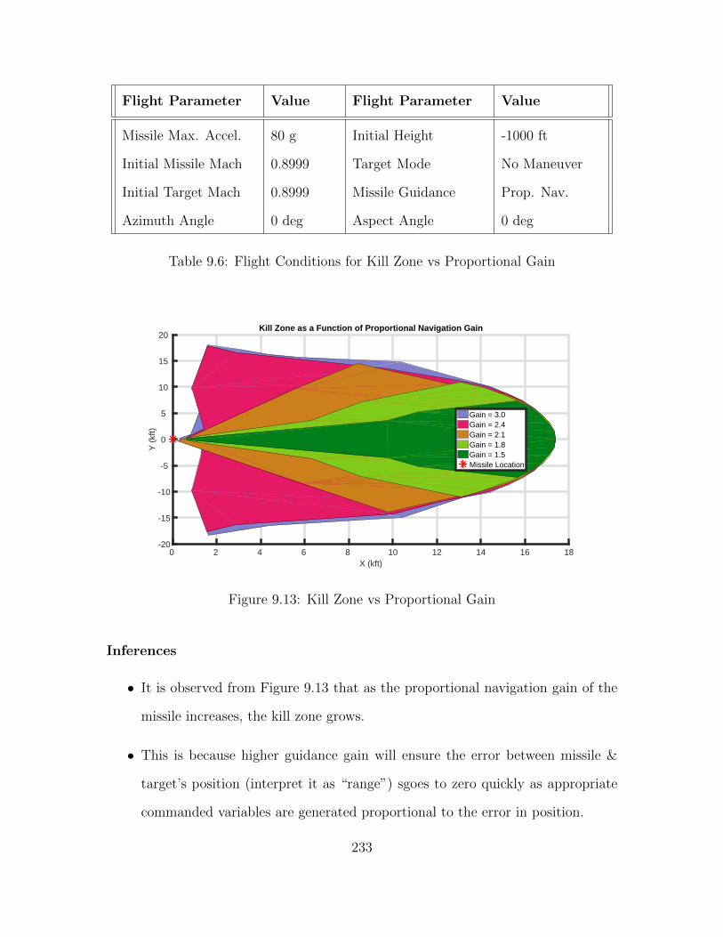
Flight Parameter Value Flight Parameter Value
Missile Max. Accel. 80 g Initial Height -1000 ft
Initial Missile Mach 0.8999 Target Mode No Maneuver
Initial Target Mach 0.8999 Missile Guidance Prop. Nav.
Azimuth Angle 0 deg Aspect Angle 0 deg
Table 9.6: Flight Conditions for Kill Zone vs Proportional Gain
X (kft)0 2 4 6 8 10 12 14 16 18
Y (
kft)
-20
-15
-10
-5
0
5
10
15
20 Kill Zone as a Function of Proportional Navigation Gain
Gain = 3.0Gain = 2.4Gain = 2.1Gain = 1.8Gain = 1.5Missile Location
Figure 9.13: Kill Zone vs Proportional Gain
Inferences
• It is observed from Figure 9.13 that as the proportional navigation gain of the
missile increases, the kill zone grows.
• This is because higher guidance gain will ensure the error between missile &
target’s position (interpret it as “range”) sgoes to zero quickly as appropriate
commanded variables are generated proportional to the error in position.
233
• The result presented above actually agrees well with the ideas explained in
section 8.2 contained in the chapter 8.
• However, there is a caveit here that the proportional gain cannot be increased
arbitrarily as a higher guidance gain will destabilize the guidance loop. This
phenomenon is captured in Figure 8.1 and the same behaviour is expected here
in kill zone estimation too.
9.9 Summary and Conclusions
In this chapter, the estimation of Kill Zone with respect to different missile/target
engagement parameters were discussed. This will give us a fair idea about when to &
when not to launch the missile when its initial conditions are known. Future research
will involve searching in 3D space with same or different algorithms. Also, a complex
target like 6DOF can be used instead of 3DOF to study the variation. This also
opens a new area of research where missile tracking multiple targets based on their
lethality and need of the hour. Thus the work done in this chapter has an excellent
scope for future research.
234

Chapter 10
MISSILE-TARGET 3D ANIMATION USING MATLAB
10.1 Introduction and Overview
The purpose of this chapter is to illustrate the design of 3D animation using
VRML toolbox in MATLAB. Earlier work done by [5] had just 2D simulation re-
sults. In order to see how a real missile would intercept its target, the need for 3D
animation arises there. MATLAB offers 3D simulation using VRML toolbox. The
objective was to connect the simulation part in MATLAB with the animation module
as described in [9]. The simulation part was coded in MATLAB with object oriented
programming design methodology and simulation updated the animation at each and
every iteration. Different viewpoints showed how the objects would move in real
time. This animation enables the visualization of missile-target engagement in real
time scenario. A key goal of the chapter is justifying the fact if the missile simulation
is going to work fine in this 3D animation, it is expected to work in real time scenario
just like it behaved in the computer simulation. As such, the chapter illustrates how
to input the inital conditions of missile and target in an interactive Graphical User
Interface(GUI) and view the real time 3D animation with all the simulation running
in the background in MATLAB.
Remainder of this chapter is organized as follows. Section 10.2 will show how
to prepare GUI, simulate the initial flight conditions. Section 10.3 will discuss the
process of updating the animation using the simulation details. Switiching between
different viewpoints is also explained here. Section 10.4 will discuss the results and
235
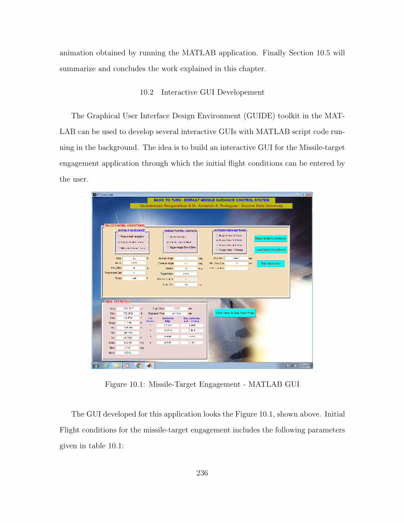
animation obtained by running the MATLAB application. Finally Section 10.5 will
summarize and concludes the work explained in this chapter.
10.2 Interactive GUI Developement
The Graphical User Interface Design Environment (GUIDE) toolkit in the MAT-
LAB can be used to develop several interactive GUIs with MATLAB script code run-
ning in the background. The idea is to build an interactive GUI for the Missile-target
engagement application through which the initial flight conditions can be entered by
the user.
Figure 10.1: Missile-Target Engagement - MATLAB GUI
The GUI developed for this application looks the Figure 10.1, shown above. Initial
Flight conditions for the missile-target engagement includes the following parameters
given in table 10.1:
236
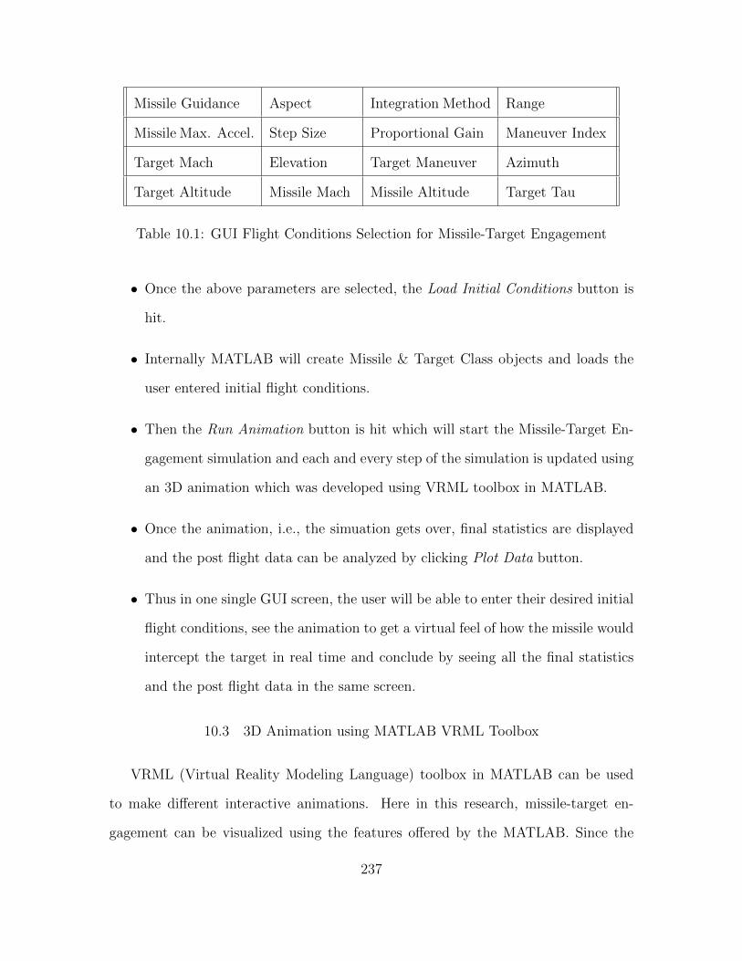
Missile Guidance Aspect Integration Method Range
Missile Max. Accel. Step Size Proportional Gain Maneuver Index
Target Mach Elevation Target Maneuver Azimuth
Target Altitude Missile Mach Missile Altitude Target Tau
Table 10.1: GUI Flight Conditions Selection for Missile-Target Engagement
• Once the above parameters are selected, the Load Initial Conditions button is
hit.
• Internally MATLAB will create Missile & Target Class objects and loads the
user entered initial flight conditions.
• Then the Run Animation button is hit which will start the Missile-Target En-
gagement simulation and each and every step of the simulation is updated using
an 3D animation which was developed using VRML toolbox in MATLAB.
• Once the animation, i.e., the simuation gets over, final statistics are displayed
and the post flight data can be analyzed by clicking Plot Data button.
• Thus in one single GUI screen, the user will be able to enter their desired initial
flight conditions, see the animation to get a virtual feel of how the missile would
intercept the target in real time and conclude by seeing all the final statistics
and the post flight data in the same screen.
10.3 3D Animation using MATLAB VRML Toolbox
VRML (Virtual Reality Modeling Language) toolbox in MATLAB can be used
to make different interactive animations. Here in this research, missile-target en-
gagement can be visualized using the features offered by the MATLAB. Since the
237

entire MATLAB application has been coded in an object oriented architecture, the
same program can be easily extended to multiple missile-target engagement just by
using new object for Missile and Target class. Thus the entire simulation data has
to be communicated to animating world in a way that it understands. Once that is
achieved, then whatever happens in simulation can be seen in real time 3D animation
as animation is just updating the simulation flow. The motivation for going for a 3D
animation is to visualize how the missile-target engagement would happen in a real
world scenario (which would be difficult for us to see in real time). And given a better
modeling and design environment, it can be believed that real missile would exactly
behave and intercept the target like it does in 3D animation. Several aerospace com-
panies spend billions of dollar in modeling the environment so that things if they
work in simulation well are expected to work almost the same way in real world.
Thus to prepare an interative 3D animation we require the following,
1. Nice and fancy 3D Background
2. Missile Object
3. Aircraft Object
4. Different Viewpoints
5. Proper interface between VRML editor and MATLAB - Could be either
through MATLAB or SIMULINK. MATLAB interface is used in this
research.
238

Figure 10.2: Missile-Target Engagement - 3D Animation
Figure 10.3: Missile-Target Engagement - 3D Animation Top View
3D World Editor - VRML Editor which comes as a part of MATLAB VRML tool-
box was used to develop the 3D animation environment. There are other commercial
VRML editors available in the market for cheaper costs like V-Realm Builder, 3DStu-
dio, Blender etc... 3D World Editor was good enough to prepare the animation in this
research. VRML files have “.wrl” format which is a short form for “world”. Initially
239

the 3D background was developed, then the missile and target objects were properly
placed in the 3D background in such a way as to mimick the initial conditions given
through the interactive MATLAB GUI. The VRML toolbox in MATLAB already
has different aerospace objects like aircraft, missile, helicopters, rockets etc. One
such missile and target aircraft from that repository is being used in this research.
Then the different viewpoints can be made according to the user requirements. A
missile cockpit viewpoint along with other 4 viewpoints were developed for this re-
search. For example, refer figure 10.3 for a top viewpoint. Cockpit viewpoint as
shown in Figure 10.2 will give a real-time feel as if we were sitting inside the missile
and riding it(Although never done in real life!). Different flight parameters of both
missile and target can be tracked as the animation progresses. This gives a real-time
feel like traveling in a fighter aircraft being a pilot. Given the power of GPUs nowa-
days, this missile-target engagement simulation can be made much faster, while the
current research is done without the usage of GPUs. Also, if the MATLAB is made
aware of intelligently using the GPUs, then this research can get really interesting.
There are other better softwares like Blender, Maya, 3DS Max which is capable of
creating content rich 3D object files in different format. As of now, good resource
files in “.wrl” format are really less available. MATLAB recently extended the 3D
animation capability to “.x3d” format too. Similarly there are ways to import 3D
object files from the 3D authoring worlds like AutoCAD, CATIA, Solidworks and so
into the MATLAB and create animations with them.
10.4 Simulation Results & Analysis
Post flight analysis from simulating the conditions from table 10.2 are plotted
and comparison of MATLAB results with C program [5] is presented. The plots
ranging from Figure 10.4 - 10.14 show that both C and MATLAB simulations are
240

really close to each other, depicting that MATLAB program is as accurate as C
program, eventhough it is written with different programming style and interpolating
techniques for calculating aerodynamic coefficients.
Flight Conditions Considered:
Flight Parameter Value Flight Parameter Value
Missile Max. Accel. 80 g Initial Height -1000 ft
Initial Missile Mach 0.8999 Target Range 2000 ft
Initial Target Mach 0.8999 Missile Guidance Optimal Control
Target Maneuver Sheldon Aspect Angle 0 deg
Table 10.2: Flight Conditions for MATLAB & C Simulations
0 0.2 0.4 0.6 0.8 1 1.2 1.40
5
10
15
20
25
30Alpha vs Flight Time
Flight Time in sec
Ang
le O
f Atta
ck in
deg
MatlabC
Figure 10.4: Alpha Profile - MATLAB & C Simulations
241

0 0.2 0.4 0.6 0.8 1 1.2 1.40
0.5
1
1.5
2
2.5
3
3.5Beta vs Flight Time
Flight Time in sec
Sid
eslip
Ang
le in
deg
MatlabC
Figure 10.5: Profile - MATLAB & C Simulations
0 0.2 0.4 0.6 0.8 1 1.2 1.40
200
400
600
800
1000
1200
1400
1600
1800
2000Range vs Flight Time
Flight Time in sec
Ran
ge in
feet
MatlabC
Figure 10.6: Profile - MATLAB & C Simulations
242
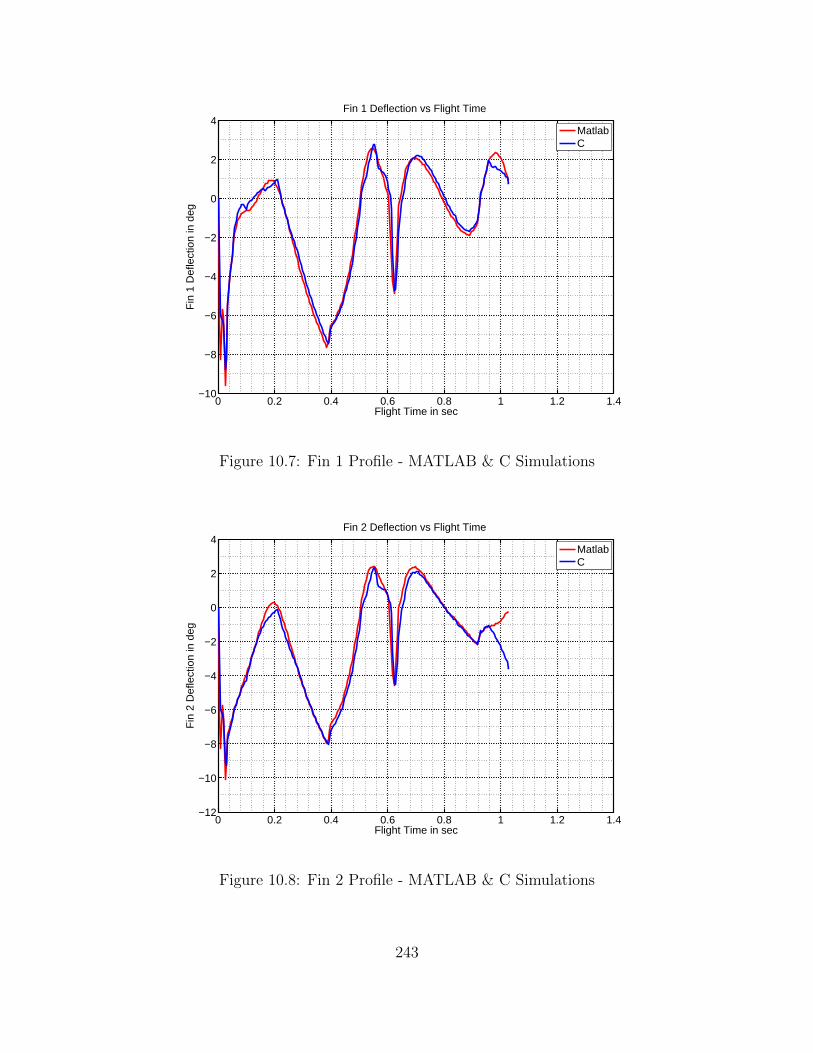
0 0.2 0.4 0.6 0.8 1 1.2 1.4−10
−8
−6
−4
−2
0
2
4Fin 1 Deflection vs Flight Time
Flight Time in sec
Fin
1 D
efle
ctio
n in
deg
MatlabC
Figure 10.7: Fin 1 Profile - MATLAB & C Simulations
0 0.2 0.4 0.6 0.8 1 1.2 1.4−12
−10
−8
−6
−4
−2
0
2
4Fin 2 Deflection vs Flight Time
Flight Time in sec
Fin
2 D
efle
ctio
n in
deg
MatlabC
Figure 10.8: Fin 2 Profile - MATLAB & C Simulations
243

0 0.2 0.4 0.6 0.8 1 1.2 1.4−6
−4
−2
0
2
4
6
8
10Fin 3 Deflection vs Flight Time
Flight Time in sec
Fin
3 D
efle
ctio
n in
deg
MatlabC
Figure 10.9: Fin 3 Profile - MATLAB & C Simulations
0 0.2 0.4 0.6 0.8 1 1.2 1.4−8
−6
−4
−2
0
2
4
6Fin 4 Deflection vs Flight Time
Flight Time in sec
Fin
4 D
efle
ctio
n in
deg
MatlabC
Figure 10.10: Fin 4 Profile - MATLAB & C Simulations
244

0 0.2 0.4 0.6 0.8 1 1.2 1.4−1400
−1200
−1000
−800
−600
−400
−200
0
200
400
600Fin 1 Rate vs Flight Time
Flight Time in sec
Fin
1 R
ate
in d
eg/s
ec
MatlabC
Figure 10.11: Fin 1 Rate Profile - MATLAB & C Simulations
0 0.2 0.4 0.6 0.8 1 1.2 1.4−1400
−1200
−1000
−800
−600
−400
−200
0
200
400
600Fin 2 Rate vs Flight Time
Flight Time in sec
Fin
2 R
ate
in d
eg/s
ec
MatlabC
Figure 10.12: Fin 2 Rate Profile - MATLAB & C Simulations
245

0 0.2 0.4 0.6 0.8 1 1.2 1.4−1000
−800
−600
−400
−200
0
200
400
600Fin 3 Rate vs Flight Time
Flight Time in sec
Fin
3 R
ate
in d
eg/s
ec
MatlabC
Figure 10.13: Fin 3 Rate Profile - MATLAB & C Simulations
0 0.2 0.4 0.6 0.8 1 1.2 1.4−1000
−800
−600
−400
−200
0
200
400
600Fin 4 Rate vs Flight Time
Flight Time in sec
Fin
4 R
ate
in d
eg/s
ec
MatlabC
Figure 10.14: Fin 4 Rate Profile - MATLAB & C Simulations
246

10.5 Summary and Conclusions
In this chapter, developement of 3D animation using MATLAB VRML toolbox is
explained in detail. Also development of interactive GUI for entering the initial flight
conditions is explained. Visualization of missile-target engagement using MATLAB
will enable us to explore future research, behaviour of both missile and target can be
studied thoroughly. Finally the MATLAB simulation results are compared with C
program [5] results and accuracy of MATLAB simulation is ascertained.
247

Chapter 11
SUMMARY & DIRECTIONS FOR FUTURE RESEARCH
11.1 Summary of Work
This thesis addressed about the analysis, and control issues that are critical about
the BTT missiles. The following summarizes key themes within the thesis.
1. Literature Survey. A fairly comprehensive literature survey of relevant work
was presented.
2. Modeling. A nonlinear dynamical model for the BTT missile was presented
and linearization analysis was performed to understand the full utility of each
model.
3. Control. Both inner-loop and outer-loop control designs were discussed in
the context of an overall hierarchical control inner-outer loop framework. This
framework lends itself to accommodate multiple phase of missile flight; The
need for an nonlinear gain scheduled autopilot was explored and a sample non-
linear autopilot was obtained using incremental nonlinear dynamic inversion
technique for the innermost rate control loop design. Comprehensive inner-loop
trade studies were conducted for the BTT missile. A great deal of effort was
spent on discussion fundamental performance limitations. Attention was spent
on numerical integration step size limitations as well as dynamic (bandwidth)
limitations.
248

4. Miss Distance Analysis. Set of missile-target engagement simulations were
carried out by varying various missile flight conditions and their effects on final
miss distance was analyzed and tabulated.
5. Kill Zone Analysis. Using Binary Search algorithm, a closed area in 2D
space where the probability of missile hitting the target being high was esti-
mated. The estimated result is analyzed for various flight parameter variations
and tabulated.
6. Animation Demonstrations. Many animation demonstrations were con-
ducted - with animation corroborating the simulation data results.
11.2 Directions for Future Research
Complicated research topic like missile control always presents great deal of fu-
ture topics to explore. Remember uncertainity modeling in plant dynamics is not
addressed here. Things get interesting when we try to include uncertainity model in
our control design and we would like to see how they affect our robustness properties
at different loop breaking points. Thus looking forward from the research conducted
here, following points will throw some light on future topics to explore.
1. Integrated Guidance Navigation & Control (GNC) design where guidance loop
is designed as a part of autopilot and the new design can be studied for its
robustness.
2. Studying missile-target engagement with a 6DOF target and learn when would
we need such a complicated target over a simple 3DOF target which is used in
this research. Remember when target is 6DOF, it will have its own autopilot.
249
3. Trying out different target intelligence algorithms and learn how an increase in
target intelligence would affect the missile’s tracking ability.
4. Extending current 2D kill zone search to 3D search space, where both missile
and target can start at any altitude. Also analyzing the same 3D kill zone
with respect to different missile-target engagement parameters and comparitive
studies can be done with 2D kill zone results presented in this thesis.
5. Optimal Control missile guidance law suffers from poor Time-To-Go estimate
problem. This can be addressed using an Extended Kalman Filter (EKF) algo-
rithm.
6. Extending one-on-one missile target engagement to multiple missile-target en-
gagement. Multiple missiles can be made to chose their target dynamically on
the run-time based on some state of emergency (need of the hour) or lethal
nature of target. This is a very interesting resource allocation problem and
interessting solutions can be achieved using game theory techniques developed
for pursuit evasion problems.
250

REFERENCES
[1] Sonne M., Rodriguez A. A., “A Viable PC Tool for the Design and Evaluationof Missile Guidance and Control Systems,” Proceedings of the American ControlConference, Baltimore, MD, June 29-July 1, 1994, pp. 2726-2730.
[2] Wallis M., Feeley J., “BTT Missile-Target Simulations on a Desktop Computer,”The Soc. for Comp. Sim. Int., 1989, pp. 79-84.
[3] Riggs T., Vergaz B., “Adv. Air-to-Air Missile Gui. Using Opt. Control and Est,”AFATL-TR-81-56 AFAL, Eglin AFB, FL.
[4] Sheldon L. C., “6DOF BTT Missile Simulations of the ILAAT Missile with Lookuptables for the Aerodynamic Coefficients,” Air force Armament Laboratory, EglinAFB, FL, 1986.
[5] Sonne M. L., Use of PC’s in Evaluation and Design of Missile Guidance andControl Systems, Arizona State University, MS Thesis, 1994.
[6] Jenniges A., Simulink Based Evaluation and Design of Missile Guidance and Con-trol Systems, Arizona State University, Independent Study Report, 1998.
[7] Cimen T., “A Generic Approach to Missile Autopilot Design using State-Dependent Nonlinear Control,” Preprints of the 18th IFAC World Congress, Mi-lano, Italy, August 28 - September 2, 2011, pp. 9587 - 9600.
[8] Siddarth A. N., Peter F., Holzapfel F., Valasek J., “Autopilot for a NonlinearNon-Minimum Phase Tail-Controlled Missile,” AIAA Guidance, Navigation, andControl Conference, 13-17 January 2014, National Harbor, Maryland.
[9] Wang G., Mei W., Liu H., Xiao Y., “The Design of Virtual Reality Flight Simula-tion Platform Based on Rigid Body Kinematics,” International Journal of DigitalContent Technology and its Applications(JDCTA), Vol. 7, No. 7, April 2013.
[10] Cloutier J. R., Stansbery D. T., “Nonlinear, Hybrid Bank-to-Turn/Skid-to-TurnMissile Autopilot Design,” Proceedings of AIAA Guidance, Navigation & ControlConference, Montreal, Canada, August 2001.
[11] Cloutier J. R., “State-Dependent Riccati Equation Techniques: An Overview,”Proceeding of American Control Conference, Albuquerque, New Mexico, June1997.
[12] Hawley P. A., Blauwkamp R. A., “Six-Degree-of-Freedom Digital Simulations forMissile Guidance, Navigation and Control,” John Hopkins APL Technical Digest,Vol. 29, No. 1, 2010.
[13] Jackson P. B., “Overview of Missile Flight Control Systems,” John Hopkins APLTechnical Digest, Vol. 29, No. 1, 2010.
251
[14] Kaplan J. A., Chappell A. R., Mcmanus J. W., “The Analysis of a Generic Air-to-Air Missile Simulation Model,” NASA Technical Memorandum 109057, June1994.
[15] Rodriguez A. A., Sonne M., “The PC as a Viable Tool in the Design and Evalu-ation Process of Guidance and Control Systems for Missiles,” Proceedings of the1994 International Conference on Simulation in Engineering Education, Tempe,AZ, January 24-26 1994, pp. 329-334.
[16] Rodriguez A. A., Aguilar R., “Graphical Visualization of Missile-Target Air-to-Air Engagements: An Educational Tool for Designing and Evaluating MissileGuidance and Control Systems,” Journal of Computer Applications in Engineer-ing Education, Vol. 3, No. 1, 1995, pp. 5-20.
[17] Rodriguez A. A., Sonne M. L., “Evaluation of Missile Guidance and ControlSystems Simulation,” The Journal of the Society for Computer Simulation, Vol.68, No. 6, June, 1997, pp. 363-376.
[18] Cloutier J. R., Evers J. H., Feeley J. J., “Assesment of Air-to-Air Missile Guid-ance and Control Technology,” IEEE Control Systems Magazine, October 1989,pp. 27-34.
[19] Silbert M., Sarkani S., Mazzuchi T., “Comparing the State Estimates of aKalman filter to a Perfect IMM Against a Maneuvering Target,” 14th Interna-tional Conference on Information Fusion, Chicago, Illinois, July 5-8, 2011, pp.1144-1148.
[20] Cronvich L. L., “Aerodynamic Considerations for Autopilot Design,” Progressin Astronautics and Aeronautics Tactical Missile Aerodynamics, Vol. 141, 1992,p. 37.
[21] Williams D. E., Friedland B., “Modern Control Theory for Design of Autopilotsfor Bank-to-Turn Missiles,” Journal Guidance Control, Vol. 10, No. 4, July-August1987, pp. 378-386.
[22] Das P., Khilar P. M., “A Randomized Searching Algorithm and its Performanceanalysis with Binary Search and Linear Search Algorithms,” The InternationalJournal of Computer Science and Applications (TIJCSA), Volume 1, No. 11, Jan2013, ISSN - 2278-1080.
[23] Hui Y., Nan Y., Chen S., Ding Q., Wu S., “Dynamic Attack Zone of Air-to-Airmissile after being launched in random wind field,” Chinese Journal of Aeronau-tics, 2015, pp. 1519 - 1528.
[24] Shinar J., Gazit R., “Optimal ‘No Escape’ Firing Envelopes of Guided Mis-siles,” AIAA Guidance Navigation & Control Conference, AIAA-paper No. 85-1960, Snowmass, Colorado, August 1985.
[25] Smith R. L., “An Autopilot Design Methodology for Bank-to-Turn Missiles,”Interim Report AFATL-TR-89-49 March 1988 - April 1989 Eglin AFB, FL.
252

[26] Kramer F. S., “Multivariable Autopilot Design and Implementation for TacticalMissiles,” American Institute of Aeronautics and Astronautics, 1998.
[27] Venkatesan R. H., Sinha N. K., “A New Guidance Law for the Defense Missile ofNonmaneuverable Aircraft,” IEEE Transactions on Control Systems Technology,Vol. 23, No. 6, November 2015.
[28] Cloutier J. R., Shamma J. S., “Gain-Scheduled Missile Autopilot Design UsingLinear Parameter Varying Transformations,” Journal of Guidance Control andDynamics, Vol. 16, No. 2, March-April 1993.
[29] Bossi J. A., Langehough M. A., “Multivariable Autopilot Designs for a Bank-to-Turn Missile,” Boeing Aerospace, Seattle.
[30] Birkmire B., “Weapon Engagement Zone Maximum Launch Range Approxima-tion Using a Multilayer Perceptron,” MS Thesis at B.S. Wright State University,2008.
[31] Chen D. Z., “Efficient Parallel Binary Search on Sorted Arrays,” (1990) Com-puter Science Technical Reports, Paper 11.
[32] Corzo C., DeHerrera M. F., Rodriguez A. A., “Missile Target Engagements: ATool for Evaluating Missile Autopilots,” Presented at the 1996 MAES NationalSymposium and Career Fair, Lake Buena Vista, FL, January 10-13, 1996.
[33] Aguilar R., Rodriguez A. A., “Graphical Visualization of Missile-Target Air-to-Air Engagements: A Tool for Designing and Evaluating Missile Guidance andControl Systems,” Presented at the 3rd NSF National Conference on Diversity inthe Scientific and Technological Workforce, October 1994.
[34] Rodriguez A. A., Wang Y., “Saturation Prevention Strategies for an UnstableBank-to-Turn (BTT) Missile: Full Information,” 13th IFAC Symposium: Au-tomatic Control in Aerospace Engineeering - Aerospace Control 1994, Editors:Schaechter D. B., Lorell K. R., Palo Alto, CA, September 12-16, 1994, pp. 149-154.
[35] Wu F., Packard A., Balas G., “LPV Control Design for Pitch- Axis MissileAutopilots,” Proceedings of the 34th Conference on Decision and Control, NewOrleans, LA, December, 1995.
[36] Balas G. J., Packard A., “Design of Robust, Time-Varying Controllers for MissileAutopilots,” Proc. 1st IEEE Conf. Control Applications, 1992.
[37] Abell D. C., Caraway W. D., “A Method for Determination of Target AspectAngle with Respect to an Unleveled Radar,” Army aviation and missile com-mand redstone arsenal al missile research development and engineering center,July 1998.
[38] Rodriguez A. A., Cloutier J. R., “Performance Enhancement for a Missile inthe Presence of Saturating Actuators,” AIAA Journal of Guidance, Control andDynamics, January-February, 1996, Vol 19, pp. 38-46.
253
[39] Rodriguez A. A., Wang Y., “Performance Enhancement for Unstable Bank-to-Turn (BTT) Missiles with Saturating Actuators,” International Journal of Con-trol, Vol. 63, No. 4, 1996, pp. 641-678.
[40] Barker J. M., Balas G. J., “Comparing Linear Parameter-Varying Gain-Scheduled Control Techniques for Active Flutter Suppression,” Journal of Guid-ance, Control and Dynamics, 23(5):948-955, September-October 2000.
[41] Rodriguez A. A., Wang Y., “Saturation Prevention Strategies for Unstable Bank-to-Turn (BTT) Missiles: Partial Information,” Proceedings of the American Con-trol Conference, Seattle, WA, June 21-23, 1995, pp. 2143-2147.
[42] Rodriguez A. A., Spillman M., Ridgely D. B., “Control of a Missile in the Pres-ence of Saturating Actuators,” Presented and Distributed at the American ControlConference, Seattle, WA, June 21-23, 1995.
[43] Puttannaiah K, Echols J, and Rodriguez A, “A Generalized H∞ Control De-sign Framework for Stable Multivariable Plants subject to Simultaneous Outputand Input Loop Breaking Specifications,” American Control Conf. (ACC), IEEE,2015.
[44] Puttannaiah K, Echols J, Mondal K and Rodriguez A, “Analysis and Use of Sev-eral Generalized H-Infinity Mixed Sensitivity Framework for Stable MultivariablePlants Subject to Simultaneous Output and Input Loop Breaking Specifications,”Accepted for publication in Conf. on Decision and Control (CDC), IEEE, 2015.
[45] Rodriguez A. A., “A Methodology for Missile Autopilot Performance Enhance-ment in the Presence of Multiple Hard Nonlinearities,” AFOSR SFRP Report,WL/MNAG, Eglin Air Force Base, FL, Sept, 1993.
[46] Rodriguez A. A., “Development of Control Design Methodologies for Flexible(High Order) Missile Systems with Multiple Hard Nonlinearities,” AFOSR SFRPReport, WL/MNAG, Eglin Air Force Base, FL, September, 1992, pp. 47-1-47-20.
[47] Johnson and Reiss, “Numerical Analysis,” Chapters 7.2.4 - 7.2.5.
[48] Arrow A., “An Analysis of Aerodynamic Requirements of Coordinated Bank-to-Turn Missiles,” NASA CR 3544, 1982.
[49] Chin S., “Missile Configuration Design,” McGraw Hill, 1961, p17.
[50] Cloutier J. et.al, “Assessment of Air-to-Air Missile Guidance and Control Tech-nology,” IEEE C. Sys., Oct 1989, pp. 27-34.
[51] Siouris G. M., “Missile Guidance and Control Systems,” 2004 Springer-VerlagNew York, Inc.
[52] Zarchan P., “Tactical and Strategic Missile Guidance,” AIAA Inc., 1990.
[53] Babister A. W., “Aircraft Stability and Control,” Oxford: Pergamon Press, 1961.
254

[54] Shastry S., Bodson M., “Adaptive Control: Stability, Convergence, and Robust-ness,” Prentice Hall, 1989.
[55] Etkin B., “Dynamics of Flight Stability and Control,” John Wiley and Sons,Inc., 1982, pp. 3.
[56] Reidel F. W., “Bank-To-Turn Control Technology Survey for Homing Missiles,”NASA CR 3325, 1980.
[57] McCormick B., “Aerodynamics, Aeronautics and Flight Mechanics,” John Wileyand Sons, Inc., 1979.
[58] Robert N., “Flight Stability and Automatic Control,” McGraw Hill, 1989, p. 6.
[59] McRuer, Duane et al., “Aircraft Dynamics and Automatic Control,” PrincetonUniversity Press, Princeton, New Jersey, 1973, p. 208.
[60] Lin, Ching-Fang, “Modern Navigation Guidance and Control Processing,” Pren-tice Hall, 1991, pp. 14, 184.
[61] Rodriguez A. A., “Missile Guidance,” Wiley Encyclopedia of Electrical and Elec-tronics Engineering, 15 June 2015.
[62] Blakelock J. H., “Automatic Control of Aircraft and Missiles,” John Wiley andSons, Inc., Second Edition.
[63] Lofberg J., “Yalmip: A toolbox for modeling and optimization in matlab inComputer Aided Control Systems Design,” 2004 IEEE International Symposium,pp. 284-289.
[64] Rodriguez A. A., Analysis and Design of Feedback Control Systems, Con-trol3D,L.L.C., Tempe, AZ, 2002.
[65] Rodriguez A. A., Analysis and Design of Multivariable Feedback Control Systems,Control3D, L.L.C., Tempe, AZ, 2002.
[66] Rodriguez A. A., Linear Systems: Analysis and Design, Control3D,L.L.C.,Tempe, AZ, 2002.
[67] Rodriguez A. A., EEE481: Computer Control Systems, course notes, 2014.
[68] Olver P., “Notes on Nonlinear Ordinary Differential Equations,”https://www.math.umn.edu/∼olver/am /odz.pdf
[69] Hespanha J. P., “Topics in Undergraduate Control Systems Design”.
[70] “Conventional Missiles Warheads and their Blast Radii,”http://kitsune.addr.com/Rifts/Rifts-Missiles/convent.htm
[71] “Wikipedia Link for Studying Binary Search Algorithm,”https://en.wikipedia.org/wiki/Binary search algorithm
255

[72] “C Program Code for Binary Search Algorithm,”http://www.programmingsimplified.com/c/source-code/c-program-binary-search
[73] “Simulink 3D Animation - User’s Guide,”http://www.mathworks.com/help/sl3d/index.html?s cid=doc ftr
[74] “Control of Linear Parameter Varying Systems - Wikipedia,”https://en.wikipedia.org/wiki/Linear parameter-varying control
[75] Gerard Leng, “MDTS Guidance, Aerodynamics & Control Course Website,”http://dynlab.mpe.nus.edu.sg/mpelsb/mdts/index.html
[76] Warnick S. C., Rodriguez A. A., “A Systematic Anti-windup Strategy and theLongitudinal Control of a Platoon of Vehicles with Control Saturations,” IEEETransactions on Vehicular Technology, Vol. 49, No. 3, May 2000, pp. 1006-101
[77] Hedrick J. K., Girard A., Control of Nonlinear Dynamic Systems: Theory andApplications, 2005.
[78] Stein G., “Respect the Unstable,” IEEE Control Systems Magazine, 2003.
[79] Skogestad S., Postlethwaite I., Multivariable Feedback Control: Analysis andDesign, Wiley, 1996.
[80] Morari M., Zafiriou E., Robust Process Control, Prentice Hall.
256

257

APPENDIX A
C CODE - BINARY SEARCH ALGORITHM
258

1 //2 // VENKATRAMAN RENGANATHAN3 // ASU ID : 12063959924 // MS EE Fa l l 2013 − Summer 20165 // Ph . No − 48062891246 // Thes is on M i s s i l e Guidance Control System7 //8 //BELOW C CODE CAN BE MODIFIED FOR MISS DISTANCE ANALYSIS TOO.9 //BINARY SEARCH KILL ZONE
1011 void main ( )12 13 in t i = 0 , up r ay f i n i s h , h i t r each , miss reach , h i t c oun t e r = 0 ;14 i n t p r ev i ou s r ay h i t c oun t = 0 , ha l f s e a r ch comp l e t e = 0 ;15 i n t r e s t a r t o n = 0 , m i s s th r e sho ld = 0 , NAN check = 0 ;16 f l o a t i n i t i a l r a n g e = 0 , miss range = 0 , f i n a l 1 8 0 h i t r a n g e = 0 ;17 f l o a t p r e v i o u s f i n a l h i t r a n g e = 0 , h i t r ange = 0 , h i t a r r a y [ 1 0 0 ] ;18 f l o a t t a r g e t h i t y p o s i t i o n s [ 1 0 0 ] , t a r g e t h i t x p o s i t i o n s [ 1 0 0 ] ;1920 a l t i t u d e a r r a y [ 0 ] = −1000;21 a l t i t u d e a r r a y [ 1 ] = −2000;22 a l t i t u d e a r r a y [ 2 ] = −5000;23 a l t i t u d e a r r a y [ 3 ] = −8000;24 a l t i t u d e a r r a y [ 4 ] = −10000;2526 max acce l ar ray [ 0 ] = 15 ;27 max acce l ar ray [ 1 ] = 30 ;28 max acce l ar ray [ 2 ] = 45 ;29 max acce l ar ray [ 3 ] = 60 ;30 max acce l ar ray [ 4 ] = 80 ;3132 /∗mach array [ 0 ] = 0 . 8999 ;33 mach array [ 1 ] = 1 . 0 ;34 mach array [ 2 ] = 1 . 1 ;35 mach array [ 3 ] = 1 . 2 ;36 mach array [ 4 ] = 1 . 3 ; ∗/3738 mach array [ 0 ] = 1 . 4 ;39 mach array [ 1 ] = 1 . 5 ;40 mach array [ 2 ] = 1 . 6 ;41 mach array [ 3 ] = 1 . 7 ;42 mach array [ 4 ] = 1 . 8 ;4344 f l i g h t c o nd i t i o n c o un t = 5 ;45 f o r ( i = 0 ; i <100; i++)46 47 // Completely c l e a r the ar rays and make them ready f o r new ray48 h i t a r r a y [ i ] = 0 ;49 t a r g e t h i t x p o s i t i o n s [ i ] = 0 ;50 t a r g e t h i t y p o s i t i o n s [ i ] = 0 ;51 5253 f o r ( mach id = 0 ; mach id <5; mach id++)54 55 a l t i i d = 0 ; //56 max acc id = 4 ; // Max ac c e l = 80g57 f l i g h t c o nd i t i o n c o un t = f l i g h t c o nd i t i o n c o un t + 1 ;58 In t i a l Cond i t i on s Count e r = 0 ; // Reset f o r every f l i g h t cond i t i on59 ray ang l e = 180 ;60 ha l f s e a r ch comp l e t e = 0 ; // r e s e t the f l a g f o r next i t e r a t i o n .61 // K i l l ZONE fo r 1 F l i gh t Condit ion62 whi le ( ray ang l e < 360 && ray ang l e > 0)63 64 i f ( h i t c oun t e r != 0)65 66 OpenOut ( ) ;67 SaveData ( h i t a r ray , t a r g e t h i t x p o s i t i o n s , t a r g e t h i t y p o s i t i o n s ) ;68 f o r ( i = 0 ; i <100; i++)69 70 // Completely c l e a r the ar rays and make them ready f o r new ray71 h i t a r r a y [ i ] = 0 ;72 t a r g e t h i t x p o s i t i o n s [ i ] = 0 ;73 t a r g e t h i t y p o s i t i o n s [ i ] = 0 ;74 75 F i l e c l o s e ( ) ;76 77 // ray search to the f a r end78 // s t o r e l a s t ray h i t counts f o r stopping the search .79 p r ev i ou s r ay h i t c oun t = h i t c oun t e r ;80 i n i t i a l r a n g e = 100 ;81 Range = i n i t i a l r a n g e ;82 h i t r ange = 0 ;83 miss range = 0 ;84 up r a y f i n i s h = 0 ;85 mi s s th r e sho ld = 0 ;86 mis s reach = 0 ;
259
87 h i t c oun t e r = 0 ;88 h i t r e a ch = 0 ;89 r e s t a r t o n = 0 ;9091 // search along 1 ray92 whi le ( u p r a y f i n i s h == 0)93 94 s l ope = tan ((180− ray ang l e )∗Deg2Rad ) ;95 f o r ( i =0; i <36; i++)96 97 X[ i ] = 0 ;98 Xdot [ i ] = 0 ;99
100 Launch ( ) ;101 F l i gh t (X, Xdot ) ; // f l y m i s s i l e , with i n i t i a l i z e d s t a t e s102 NAN check = ( ( Range != Range ) | | (Smx != Smx ) ) ;103 i f ( r e s t a r t o n == 0) // normal search i s happening104 105 i f ( ( Range <= 20 && Range >= 0) && miss reach != 1)106 107 // h i t cond i t i on be f o r e 1 s t miss along ray108 h i t r e a ch = 1 ;109 mi s s th r e sho ld = 0 ;110 h i t r ange = i n i t i a l r a n g e ;111 h i t a r r a y [ h i t c oun t e r ] = h i t r ange ;112 t a r g e t h i t x p o s i t i o n s [ h i t c oun t e r ] = t a r g e t i n i t i a l x ;113 t a r g e t h i t y p o s i t i o n s [ h i t c oun t e r ] = t a r g e t i n i t i a l y ;114 h i t c oun t e r = h i t c oun t e r + 1 ;115 i n i t i a l r a n g e = 2 ∗ h i t r ange ;116 Range = i n i t i a l r a n g e ;117 118 e l s e i f ( ( Range <= 20 && Range >= 0) && miss reach == 1)119 120 // h i t cond i t i on a f t e r 1 s t miss along ray121 h i t r e a ch = 1 ;122 mi s s th r e sho ld = 0 ;123 h i t r ange = i n i t i a l r a n g e ;124 h i t a r r a y [ h i t c oun t e r ] = h i t r ange ;125 t a r g e t h i t x p o s i t i o n s [ h i t c oun t e r ] = t a r g e t i n i t i a l x ;126 t a r g e t h i t y p o s i t i o n s [ h i t c oun t e r ] = t a r g e t i n i t i a l y ;127 h i t c oun t e r = h i t c oun t e r + 1 ;128 i n i t i a l r a n g e = ( h i t r ange + miss range ) /2 ;129 Range = i n i t i a l r a n g e ;130 131 e l s e i f ( ( ( fabs (Range ) > 20) | | (NAN check == 1)) && ( h i t r e a ch != 1))132 133 // miss cond i t i on be f o r e 1 s t h i t134 mis s reach = 1 ;135 mi s s th r e sho ld = mi s s th r e sho ld + 1 ;136 miss range = i n i t i a l r a n g e ;137 i n i t i a l r a n g e = 2∗ miss range ;138 Range = i n i t i a l r a n g e ;139 140 e l s e i f ( ( ( fabs (Range ) > 20) | | (NAN check == 1)) && ( h i t r e a ch == 1))141 142 // miss cond i t i on a f t e r 1 s t h i t143 mis s reach = 1 ;144 mi s s th r e sho ld = mi s s th r e sho ld + 1 ;145 miss range = i n i t i a l r a n g e ;146 i n i t i a l r a n g e = ( h i t r ange + miss range ) / 2 ;147 Range = i n i t i a l r a n g e ;148 149 150 e l s e // r e s t a r t i s happening151 152 i f ( ( Range <= 20 && Range >= 0) && miss reach != 1)153 154 // h i t cond i t i on whi le querying range us ing155 // p r e v i o u s r a y f i n a l h i t r a n g e156 h i t r e a ch = 1 ;157 mi s s th r e sho ld = 0 ;158 h i t r ange = i n i t i a l r a n g e ;159 h i t a r r a y [ h i t c oun t e r ] = h i t r ange ;160 t a r g e t h i t x p o s i t i o n s [ h i t c oun t e r ] = t a r g e t i n i t i a l x ;161 t a r g e t h i t y p o s i t i o n s [ h i t c oun t e r ] = t a r g e t i n i t i a l y ;162 h i t c oun t e r = h i t c oun t e r + 1 ;163 i n i t i a l r a n g e = 2 ∗ h i t r ange ;164 Range = i n i t i a l r a n g e ;165 166 e l s e i f ( ( Range <= 20 && Range >= 0) && miss reach == 1)167 168 // h i t cond i t i on a f t e r 1 s t miss along ray169 h i t r e a ch = 1 ;170 mi s s th r e sho ld = 0 ;171 h i t r ange = i n i t i a l r a n g e ;172 h i t a r r a y [ h i t c oun t e r ] = h i t r ange ;173 t a r g e t h i t x p o s i t i o n s [ h i t c oun t e r ] = t a r g e t i n i t i a l x ;174 t a r g e t h i t y p o s i t i o n s [ h i t c oun t e r ] = t a r g e t i n i t i a l y ;
260

175 h i t c oun t e r = h i t c oun t e r + 1 ;176 i n i t i a l r a n g e = ( h i t r ange + miss range ) /2 ;177 Range = i n i t i a l r a n g e ;178 179 e l s e i f ( ( fabs (Range ) > 20) | | (NAN check == 1))180 181 // miss cond i t i on whi le querying range us ing182 // p r e v i o u s r a y f i n a l h i t r a n g e183 mis s reach = 1 ;184 mi s s th r e sho ld = mi s s th r e sho ld + 1 ;185 miss range = i n i t i a l r a n g e ;186 i n i t i a l r a n g e = ( h i t r ange + miss range ) / 2 ;187 Range = i n i t i a l r a n g e ;188 189 // r e s t a r t module completed190 i f ( ( m i s s th r e sho ld >= 10) && ( h i t r e a ch == 0))191 192 // FINAL TERMINATION CRITERION193 up r a y f i n i s h = 1 ; // ray search over194 195 i f ( ( fabs ( h i t r ange − miss range ) < 100) && ( up r a y f i n i s h == 0))196 // | hit−miss |<100 | | range>20197 i f ( miss range > h i t r ange )198 199 // FINAL TERMINATION CRITERION200 up r a y f i n i s h = 1 ; // ray search over201 202 e l s e203 204 // I n i t i a l Hit Range found .205 // Restart the a lgor i thm to f i nd the f i n a l h i t r ange206 // FORCE RESTART207 i f ( r ay ang l e == 180)208 209 i n i t i a l r a n g e = 2 ∗ h i t a r r a y [ 0 ] ;210 211 e l s e212 213 // search cur rent ray ' s f i n a l h i t p o s i t i o n with214 // idea from prev ious ray ' s f i n a l h i t p o s i t i o n215 i n i t i a l r a n g e = p r e v i o u s f i n a l h i t r a n g e ;216 217 h i t r ange = h i t a r r a y [ 0 ] ;218 h i t r e a ch = 0 ; // r e s e t h i t r e a ch f l a g219 mis s reach = 0 ; // r e s e t mis s reach f l a g220 up r a y f i n i s h = 0 ; // ray search not over221 Range = i n i t i a l r a n g e ;222 r e s t a r t o n = 1 ;223 224 225 // CHECK FOR TERMINATION CRITERION FOR BOTTOM AND TOP SEARCH226 i f ( u p r a y f i n i s h == 1)227 228 i f ( h i t c oun t e r == 0 && pr ev i ou s r ay h i t c oun t != 0229 && ha l f s e a r ch comp l e t e == 0)230 231 // FINAL TERMINATION CRITERION fo r BOTTOM SEARCH232 // h i t c oun t e r == 0 −−−> cur rent ray i s a complete miss ing ray233 // p r ev i ou s r ay h i t c oun t != 0 −−−> prev ious ray had a t l e a s t 1 h i t234 // ha l f s e a r ch comp l e t e == 0 −−> bottom search i s happenning235 // Previous ray had a t l e a s t 1 h i t and current ray has no h i t s .236 // Stop sea rch ing along ray which cont inuous ly g i v e s a miss237 // f o r c e i t to s t a r t s ea r ch ing from 178 deg in the top d i r e c t i o n238 // s e t the bottom search complete f l a g to 1239 up r a y f i n i s h = 1 ;240 ray ang l e = 180 ;241 p r e v i o u s f i n a l h i t r a n g e = f i n a l 1 8 0 h i t r a n g e ;242 ha l f s e a r ch comp l e t e = 1 ;243 244 e l s e i f ( h i t c oun t e r == 0 && pr ev i ou s r ay h i t c oun t != 0245 && ha l f s e a r ch comp l e t e == 1)246 247 // FINAL TERMINATION CRITERION fo r TOP SEARCH248 // h i t c oun t e r == 0 −−−> cur rent ray i s a complete miss ing ray249 // p r ev i ou s r ay h i t c oun t != 0 −−−> prev ious ray had a t l e a s t 1 h i t250 // ha l f s e a r ch comp l e t e == 1 −−> top search i s happenning251 // Previous ray had a t l e a s t 1 h i t and current ray has no h i t s .252 up r a y f i n i s h = 1 ;253 // Stop sea rch ing along ray which cont inuous ly g i v e s a miss254 ray ang l e = 500 ;255 // Stop K i l l Zone Search − big number to get out o f both the loops256 257 258 // ray search ge t s over here259
261

260 // DECIDING HOW TO PROCEED TO NEXT RAY261 i f ( ha l f s e a r ch comp l e t e == 0)262 263 // increment bottom search ray angle by 10 degree264 i f ( r ay ang l e == 180)265 266 f i n a l 1 8 0 h i t r a n g e = h i t a r r a y [ h i t c oun t e r − 1 ] ;267 p r e v i o u s f i n a l h i t r a n g e = f i n a l 1 8 0 h i t r a n g e ;268 269 e l s e270 271 p r e v i o u s f i n a l h i t r a n g e = h i t a r r a y [ h i t c oun t e r − 1 ] ;272 273 ray ang l e = ray ang l e + 5 ;274 275 e l s e // ha l f s e a r ch comp l e t e == 1276 277 // decrement top search ray angle by 10 degree278 i f ( r ay ang l e != 180)279 280 p r e v i o u s f i n a l h i t r a n g e = h i t a r r a y [ h i t c oun t e r − 1 ] ;281 282 ray ang l e = ray ang l e − 5 ;283 284 285 // end o f FOR LOOP286 return ; /∗ . . . and return ∗/287
1 %% DATA PREPARE SIMPLE.M2 %% PREPARE KILL ZONE DAT FILES FOR PLOTTING3 range f i l ename = ' out range .da t ' ;4 s t x f i l e n ame = ' ou t s t x . da t ' ;5 s t y f i l e n ame = ' ou t s t y . da t ' ;6 f i l e name 1 = ' S imu la t i on Resu l t s / Fl ight Cdtn ' ;7 f o r i = 6 :108 % i = 1 ;9 f l i ght number path = s t r c a t ( f i l e name 1 , num2str ( i ) ) ;
10 cd ( f l i ght number path ) ;11 f i l e s t r u c t = d i r ;12 numdi rec tor i e s ( i ) = sum ( [ f i l e s t r u c t . i s d i r ] ) − 2 ;13 cd . .14 cd . .15 end1617 f o r k = 6:1018 % f o r each and every ray − each ray i s an i n i t i a l cond i t i on19 f o r i = 1 : numdi rec to r i e s ( k )20 sim number = num2str ( i ) ;21 f l t cdtn number = num2str (k ) ;22 f l i ght number path = s t r c a t ( f i l e name 1 , f l t cdtn number ) ;23 f i l e name 2 = ' / Simulated IC ' ;24 f i l e name 3 = ' Resu l t s ' ;25 fo lder name = s t r c a t ( f l i ght number path , f i l e name 2 , . . .26 sim number , f i l e name 3 ) ;27 cd ( fo lder name ) ;2829 f i l e ID = fopen ( range f i l ename , ' r+b ' ) ;30 temp h i t range ar ray = f read ( f i l e ID , 50000 , ' ∗ f l o a t ' ) ;31 f c l o s e ( f i l e ID ) ;3233 f i l e ID = fopen ( s tx f i l e name , ' r+b ' ) ;34 t emp h i t s tx a r r ay = f read ( f i l e ID , 50000 , ' ∗ f l o a t ' ) ;35 f c l o s e ( f i l e ID ) ;3637 f i l e ID = fopen ( s ty f i l e name , ' r+b ' ) ;38 t emp h i t s ty a r r ay = f read ( f i l e ID , 50000 , ' ∗ f l o a t ' ) ;39 f c l o s e ( f i l e ID ) ;40 cd . .41 cd . .42 cd . .4344 % Prepare exact array from big array which has l o t o f z e ro s45 f o r j = 1 : l ength ( t emp h i t s t x a r r ay )46 i f ( t emp h i t range ar ray ( j ) > 0)47 h i t r ang e a r r ay ( j ) = temp h i t range ar ray ( j ) ;48 h i t s t x a r r a y ( j ) = temp h i t s tx a r r ay ( j ) ;49 h i t s t y a r r a y ( j ) = temp h i t s ty a r r ay ( j ) ;50 end51 end5253 [ min range , min index ] = min ( h i t r ang e a r r ay ) ;54 [ max range , max index ] = max( h i t r ang e a r r ay ) ;55 i n i t i a l h i t x ( i ) = h i t s t x a r r a y ( min index ) ;
262

56 i n i t i a l h i t y ( i ) = h i t s t y a r r a y ( min index ) ;57 f i n a l h i t x ( i ) = h i t s t x a r r a y (max index ) ;58 f i n a l h i t y ( i ) = h i t s t y a r r a y (max index ) ;5960 c l e a r t emp h i t range ar ray ;61 c l e a r t emp h i t s tx a r r ay ;62 c l e a r t emp h i t s ty a r r ay ;63 c l e a r h i t r ang e a r r ay ;64 c l e a r h i t s t x a r r a y ;65 c l e a r h i t s t y a r r a y ;6667 end6869 h i t x = [ i n i t i a l h i t x ' ; f i n a l h i t x ' ] ;70 h i t y = [ i n i t i a l h i t y ' ; f i n a l h i t y ' ] ;71 da t f i l e name = s t r c a t ( ' k i l l z o n e ' , f l t cdtn number , ' data.mat ' ) ;72 cd ( ' Ki l l Zone Dat F i l e s ' ) ;73 save ( da t f i l e name ) ;74 cd . .75 end
1 %% PLOT KILL ZONE.M2 c l e a r a l l ; c l c ;3 f o r l = 9:−1:14 name 1 = ' k i l l z o n e ' ;5 name 2 = ' data.mat ' ;6 data num = num2str ( l ) ;7 f i l e name = s t r c a t ( name 1 , data num , name 2 ) ;8 load ( f i l e name ) ;9 A = double ( h i t x ) ;
10 B = double ( h i t y ) ;11 k = boundary (A,B) ;12 switch ( l )13 case 114 c o l o r v e c t o r = [0 . 5 . 1 ] ;15 case 216 c o l o r v e c t o r = [ . 5 . 8 . 1 ] ;17 case 318 c o l o r v e c t o r = [ . 8 . 5 . 1 ] ;19 case 420 c o l o r v e c t o r = [ . 9 . 1 . 4 ] ;21 case 522 c o l o r v e c t o r = [ . 5 . 5 . 8 ] ;23 case 624 c o l o r v e c t o r = [ . 5 0 . 1 ] ;25 case 726 c o l o r v e c t o r = [0 . 1 0 . 9 0 . 2 ] ;27 case 828 c o l o r v e c t o r = [0 . 8 0 . 8 0 . 1 ] ;29 case 930 c o l o r v e c t o r = [0 . 1 0 . 2 0 . 3 ] ;31 case 1032 c o l o r v e c t o r = [0 . 9 0 . 8 0 . 7 ] ;33 end34 patch (A(k ) ,B(k ) , c o l o r v e c t o r )35 hold on ;36 end3738 p lo t (0 ,0 , ' r ∗ ' , ' MarkerSize ' , 20)39 hold on ;404142 gr id on ;43 t i t l e ( ' Ki l l Zone as a Function o f I n i t i a l M i s s i l e Mach ' , ' f o n t s i z e ' , 24)44 legend ( 'Mach = 1 .7 ' , 'Mach = 1 .6 ' , 'Mach = 1 .5 ' , 'Mach = 1 .4 ' , . . .45 'Mach = 1 .3 ' , 'Mach = 1 .2 ' , 'Mach = 1 .1 ' , 'Mach = 1 .0 ' , . . .46 'Mach = 0 .8999 ' , ' Mi s s i l e Locat ion ' , ' Locat ion ' , ' Best ' ) ;47 s e t ( gcf , ' PaperPositionMode ' , ' auto ' ) ;48 s e t ( f i ndob j ( gca , ' type ' , ' l i n e ' ) , 'LineWidth ' , 2 ) ;49 h = f i ndob j ( gcf , ' type ' , ' l i n e ' ) ;50 s e t (h , 'LineWidth ' , 3 ) ;51 a = f i ndob j ( gcf , ' type ' , ' axes ' ) ;52 s e t ( a , ' l i n ew idth ' , 6 ) ;53 ax = gca ;54 x vec to r = 0 : 5 : 2 5 ;55 y vec to r = −25:5 :25 ;56 s e t ( ax , 'XTickLabel ' , x vec to r )57 s e t ( ax , 'YTickLabel ' , y vec to r )58 s e t (a , ' FontSize ' , 2 4 ) ;59 hold o f f60 x l ab e l ( 'X ( k f t ) ' , ' f o n t s i z e ' , 2 4 ) ;61 y l ab e l ( 'Y ( k f t ) ' , ' f o n t s i z e ' , 2 4 ) ;
263

APPENDIX B
MATLAB CODE - MISSILE PLANT & AUTOPILOT ANALYSIS
264

1 %========================================================================+2 % M− f i l e ” b t t l i n r .m ” SOLVES FOR THE NON−DIMENSIONAL STABILITY3 % DERIVATIVES OF THE NON−DIMENSIONAL ( i . e . , SCALED) STATE−SPACE SYSTEM.4 % THIS M−FILE ALSO FORMS THE A, B, C & D STATE−SPACE MATRICES OF5 % LINEAR MODEL.6 %7 % Written by : Venkatraman Renganathan8 % −−−−−−−−−−− (480)628−9124 (Mobile Number) %9 %========================================================================+
1011 %∗∗∗∗∗∗∗∗∗∗∗∗∗∗∗∗∗∗∗∗∗∗∗∗∗∗∗∗∗∗∗∗∗∗∗∗∗∗∗∗∗∗∗∗∗∗∗∗∗∗∗∗∗∗∗∗∗∗∗∗∗∗∗∗∗∗∗∗∗∗∗12 % Reference ( trim va lues ) Inputs to the L i n e r i z a t i o n Procedure :13 %∗∗∗∗∗∗∗∗∗∗∗∗∗∗∗∗∗∗∗∗∗∗∗∗∗∗∗∗∗∗∗∗∗∗∗∗∗∗∗∗∗∗∗∗∗∗∗∗∗∗∗∗∗∗∗∗∗∗∗∗∗∗∗∗∗∗∗∗∗∗∗14 mach array = [1 .068 1 .5114 2 .0420 ] ;15 th ru s t a r r ay = [600 1400 2000 ] ;16 mach length = length ( mach array ) ;1718 f o r j j =1:21920 a l t i t r e f = 30000 .00 ; % Mi s s i l e Geometric Al t i tude Reference Value [ f t ]21 a l pha r e f = 14 ; % Mi s s i l e Angle o f Attack Reference Value [ deg ]22 b e t a r e f = 0 . 0 ; % Mi s s i l e Side−s l i p Reference Value [ deg ]23 d e lP r e f = 0 . 0 ; % ”Rol l ” Fin De f l e c t i on Reference Value [ deg ]24 de lR r e f = 0 . 0 ; % ”Yaw” Fin De f l e c t i on Reference Value [ deg ]25 P re f = 0 . 0 ; % Rol l Rate Reference Value [ rad/ s ]26 Q re f = 0 . 0 ; % Pitch Rate Reference Value [ rad/ s ]27 R re f = 0 . 0 ; % Yaw Rate Reference Value [ rad/ s ]28 Ph i r e f = 0 . 0 ; % Bank Angle Reference Value [ deg ]29 Theta re f = 0 . 0 ; % Att i tude Angle [ deg ]30 P s i r e f = 0 . 0 ; % Heading Angle [ deg ]31 ThrustX = th ru s t a r r ay ( j j ) ; % Sea Level 2nd Stage Thrust Force in32 % the Body X−d i r e c t i o n [ l b f ]3334 %∗∗∗∗∗∗∗∗∗∗∗∗∗∗∗∗∗∗∗∗∗∗∗∗∗∗∗∗∗∗∗∗∗∗∗∗∗∗∗∗∗∗∗∗∗∗∗∗∗∗∗∗∗∗∗∗∗∗∗∗∗∗∗∗∗∗∗∗∗∗∗35 % Actuator Dynamics ( parameters ) :36 %∗∗∗∗∗∗∗∗∗∗∗∗∗∗∗∗∗∗∗∗∗∗∗∗∗∗∗∗∗∗∗∗∗∗∗∗∗∗∗∗∗∗∗∗∗∗∗∗∗∗∗∗∗∗∗∗∗∗∗∗∗∗∗∗∗∗∗∗∗∗∗37 KdelP = 1 .0 ; % E f f e c t i v e ”Rol l ” actuator c losed−loop gain38 KdelR = 1 .0 ; % E f f e c t i v e ”Yaw” actuator c losed−loop gain39 KdelQ = 1 .0 ;40 tau delP = .005 ; % E f f e c t i v e ”Rol l ” Actuator time constant [ s ec ]41 tau delR = .005 ; % E f f e c t i v e ”Yaw” Actuator time constant [ s ec ]42 tau delQ = .005 ; % E f f e c t i v e ”Pitch ” Actuator time constant [ s ec ]4344 %∗∗∗∗∗∗∗∗∗∗∗∗∗∗∗∗∗∗∗∗∗∗∗∗∗∗∗∗∗∗∗∗∗∗∗∗∗∗∗∗∗∗∗∗∗∗∗∗∗∗∗∗∗∗∗∗∗∗∗∗∗∗∗∗∗∗∗∗∗∗∗45 % Set Aerodynamic Co e f f i c i e n t I t e r a t i o n Loop Absolute Error C r i t e r i a46 %∗∗∗∗∗∗∗∗∗∗∗∗∗∗∗∗∗∗∗∗∗∗∗∗∗∗∗∗∗∗∗∗∗∗∗∗∗∗∗∗∗∗∗∗∗∗∗∗∗∗∗∗∗∗∗∗∗∗∗∗∗∗∗∗∗∗∗∗∗∗∗47 e r r c r i t = 0 .005 ;4849 %∗∗∗∗∗∗∗∗∗∗∗∗∗∗∗∗∗∗∗∗∗∗∗∗∗∗∗∗∗∗∗∗∗∗∗∗∗∗∗∗∗∗∗∗∗∗∗∗∗∗∗∗∗∗∗∗∗∗∗∗∗∗∗∗∗∗∗∗∗∗∗50 % Other Aerodynamic , Mass , and I n e r t i a Parameters :51 %∗∗∗∗∗∗∗∗∗∗∗∗∗∗∗∗∗∗∗∗∗∗∗∗∗∗∗∗∗∗∗∗∗∗∗∗∗∗∗∗∗∗∗∗∗∗∗∗∗∗∗∗∗∗∗∗∗∗∗∗∗∗∗∗∗∗∗∗∗∗∗52 Lre f = 0 .625 ; % Aerodynamic Reference Length [ f t ]53 S r e f = 0 .307 ; % Aerodynamic Reference Area [ f t ˆ2 ]54 mass = 5 .75 ; % Mi s s i l e Mass [ s lug ]55 Ixx = 0 .34 ; % Mi s s i l e Body Frame X−Comp. o f I n e r t i a ( Fuel Spent ) :56 Iyy = 34 .10 ; % Mi s s i l e Body Frame X−Comp. o f Mass Moment [ s lug / f t ˆ2 ]57 I z z = 34 .10 ; % Mi s s i l e Body Frame X−Comp. o f Mass Moment [ s lug / f t ˆ2 ]58 xcg = 0 .0 ; %.525 Fina l Locat ion o f Center o f Mass [ f t ]5960 %∗∗∗∗∗∗∗∗∗∗∗∗∗∗∗∗∗∗∗∗∗∗∗∗∗∗∗∗∗∗∗∗∗∗∗∗∗∗∗∗∗∗∗∗∗∗∗∗∗∗∗∗∗∗∗∗∗∗∗∗∗∗∗∗∗∗∗∗∗∗∗61 % Calcu la te Atmospheric Prope r t i e s :62 %∗∗∗∗∗∗∗∗∗∗∗∗∗∗∗∗∗∗∗∗∗∗∗∗∗∗∗∗∗∗∗∗∗∗∗∗∗∗∗∗∗∗∗∗∗∗∗∗∗∗∗∗∗∗∗∗∗∗∗∗∗∗∗∗∗∗∗∗∗∗∗63 % [ rho , SOS,Patm ,Tatm , grav i ty , drho dz , dSOS dz ] = atmos ( abs ( a l t i t r e f ) ) ;64 [ rho , SOS, g rav i ty ] = Compute Altitude Parameters ( a l t i t r e f ) ;6566 %∗∗∗∗∗∗∗∗∗∗∗∗∗∗∗∗∗∗∗∗∗∗∗∗∗∗∗∗∗∗∗∗∗∗∗∗∗∗∗∗∗∗∗∗∗∗∗∗∗∗∗∗∗∗∗∗∗∗∗∗∗∗∗∗∗∗∗∗∗∗∗67 % In t e r a t e f o r Mach Number , de lQ re f , and Aerodynamic Co e f f i c i e n t s :68 %∗∗∗∗∗∗∗∗∗∗∗∗∗∗∗∗∗∗∗∗∗∗∗∗∗∗∗∗∗∗∗∗∗∗∗∗∗∗∗∗∗∗∗∗∗∗∗∗∗∗∗∗∗∗∗∗∗∗∗∗∗∗∗∗∗∗∗∗∗∗∗6970 %======================================================71 % Correct Sea Level Thrust f o r Al t i tude ( a i r dens i ty ) :72 %======================================================73 rho sea = 0 .0024 ; % Sea Level Air Density [ s lug / f t 3 ]74 ThrustX = ThrustX ∗( rho/ rho sea ) ; % Corrected Propu l s ive Thrust [ l b f ]7576 %=======================================================77 % Load Aerodynamic Tables ( execute m− f i l e ” aerodat.m ” ) :78 %=======================================================79 aerodat8081 %================================82 % Guess Mach Number and de lQ re f83 %================================84 Mach ref = mach array ( j j ) ;85 de lQ re f = 1 . 0 ; % [ deg ]
265

86 e r r o r = 1 .0 ;87 icount = 0 ;8889 %======================90 % Begin I t e r a t i o n Loop91 %======================92 whi le e r r o r > e r r c r i t9394 Vb = SOS∗Mach ref ;95 Vb old = Vb;9697 % Use Absolute Values o f Alpha re f and Beta r e f f o r most I n t e r p o l a t i o n s :98 absAlp = abs ( a l pha r e f ) ;99 absBet = abs ( b e t a r e f ) ;
100101 % Use ”Pitch ” Fin De f l e c t i on to Determine Sign o f delQAlp :102 i f d e lQ re f >= 0 .0103 delQAlp = abs ( a l pha r e f ) ;104 e l s e105 delQAlp = −1. 0 ∗abs ( a l pha r e f ) ;106 end107108 % Use ”Yaw” Fin De f l e c t i on to Determince Sign o f delRBet :109 i f d e lR r e f >= 0 .0110 delRBet = abs ( b e t a r e f ) ;111 e l s e112 delRBet = −1. 0 ∗abs ( b e t a r e f ) ;113 end114115 %========================================================================116 % In t e r po l a t e f o r Drag Co e f f i c i e n t CD=CD( alpha , delQ ,M) :117 % CD i s a three dimens ional array in a c t u a l i t y ; however , MATLAB only118 % supports i n t e r p o l a t i o n o f 2−D Table s . Thus , we w i l l car ry out 2−D119 % in t e r p o l a t i o n between a fami ly o f 2−D tab l e s in the x and y d i r e c t i o n s120 % ( alpha and delQ , r e s p e c t i v e l y ) and then l i n e a r l y i n t e r p o l a t e between121 % these two va lues f o r the f i n a l z−d i r e c t i o n (Mach number ) :122 %========================================================================123 i f Mach ref <= 1 .0124 Mach lo = 0 .9 ;125 Mach hi = 1 .0 ;126 CDlo = inte rp2 (TdelQ ' , Talpha1 ,TCD1, de lQ re f , absAlp , ' b i l i n e a r ' ) ;127 CDhi = in t e rp2 (TdelQ ' , Talpha1 ,TCD2, de lQ re f , absAlp , ' b i l i n e a r ' ) ;128129 e l s e i f Mach ref <= 1 .1130 Mach lo = 1 .0 ;131 Mach hi = 1 .1 ;132 CDlo = inte rp2 (TdelQ ' , Talpha1 ,TCD2, de lQ re f , absAlp , ' b i l i n e a r ' ) ;133 CDhi = in t e rp2 (TdelQ ' , Talpha1 ,TCD3, de lQ re f , absAlp , ' b i l i n e a r ' ) ;134135 e l s e i f Mach ref <= 1 .3136 Mach lo = 1 .1 ;137 Mach hi = 1 .3 ;138 CDlo = inte rp2 (TdelQ ' , Talpha1 ,TCD3, de lQ re f , absAlp , ' b i l i n e a r ' ) ;139 CDhi = in t e rp2 (TdelQ ' , Talpha1 ,TCD4, de lQ re f , absAlp , ' b i l i n e a r ' ) ;140141 e l s e i f Mach ref <= 1 .5142 Mach lo = 1 .3 ;143 Mach hi = 1 .5 ;144 CDlo = inte rp2 (TdelQ ' , Talpha1 ,TCD4, de lQ re f , absAlp , ' b i l i n e a r ' ) ;145 CDhi = in t e rp2 (TdelQ ' , Talpha1 ,TCD5, de lQ re f , absAlp , ' b i l i n e a r ' ) ;146147 e l s e i f Mach ref <= 2 .0148 Mach lo = 1 .5 ;149 Mach hi = 2 .0 ;150 CDlo = inte rp2 (TdelQ ' , Talpha1 ,TCD5, de lQ re f , absAlp , ' b i l i n e a r ' ) ;151 CDhi = in t e rp2 (TdelQ ' , Talpha1 ,TCD6, de lQ re f , absAlp , ' b i l i n e a r ' ) ;152153 e l s e i f Mach ref <= 2 .5154 Mach lo = 2 .0 ;155 Mach hi = 2 .5 ;156 CDlo = inte rp2 (TdelQ ' , Talpha1 ,TCD6, de lQ re f , absAlp , ' b i l i n e a r ' ) ;157 CDhi = in t e rp2 (TdelQ ' , Talpha1 ,TCD7, de lQ re f , absAlp , ' b i l i n e a r ' ) ;158159 e l s e i f Mach ref <= 3 .0160 Mach lo = 2 .5 ;161 Mach hi = 3 .0 ;162 CDlo = inte rp2 (TdelQ ' , Talpha1 ,TCD7, de lQ re f , absAlp , ' b i l i n e a r ' ) ;163 CDhi = in t e rp2 (TdelQ ' , Talpha1 ,TCD8, de lQ re f , absAlp , ' b i l i n e a r ' ) ;164165 e l s e i f Mach ref <= 4 .0166 Mach lo = 3 .0 ;167 Mach hi = 4 .0 ;168 CDlo = inte rp2 (TdelQ ' , Talpha1 ,TCD8, de lQ re f , absAlp , ' b i l i n e a r ' ) ;169 CDhi = in t e rp2 (TdelQ ' , Talpha1 ,TCD9, de lQ re f , absAlp , ' b i l i n e a r ' ) ;170 end171172 % In t e r p l o a t e in the z−d i r e c t i o n (Mach ) : L inea r ly i n t e r p o l a t e between173 % the two i n t e rpo l a t ed t ab l u l a r va lues CDlo and CDhi.174 vv = (Mach ref − Mach lo )/( Mach hi − Mach lo ) ;175 CD = (1 . 0 − vv )∗CDlo + vv∗CDhi ;
266

176177178 %===================================================================179 % In t e r po l a t e f o r the Other Aerodynamic Co e f f i c i e n t s :180 % (NOTE: I n t e r p o l a t i o n func t i on s r e qu i r e that r e f e r e n c e v a r i a b l e s181 % [ e . g . , Mach ref , a lpha r e f , e t c . ] l i e with in the tabu la r va lues −182 % an e r r o r w i l l occur i f t h i s i s not the case )183 %===================================================================184185 %===========================186 % CDT = CDT(M) :187 %===========================188 CDT = inte rp1 (Tmach2 ,TCDT, Mach ref ) ;189190 %===========================191 % CLbeta = CLbeta ( alpha ,M) :192 %===========================193 CLbeta = inte rp2 (Tmach1 ' , Talpha1 , TCLbeta , Mach ref , absAlp , ' b i l i n e a r ' ) ;194195 %===========================196 % CLdelP = CLdelP ( alpha ,M) :197 %===========================198 CLdelP = inte rp2 (Tmach1 ' , Talpha1 , TCLdelP , Mach ref , absAlp , ' b i l i n e a r ' ) ;199200 %===========================201 % CLP = CLP( alpha ,M) :202 %===========================203 CLP = inte rp2 (Tmach1 ' , Talpha3 ,TCLP, Mach ref , absAlp , ' b i l i n e a r ' ) ;204205 %=============================206 % CMalpha = CMalpha( alpha ,M) :207 %=============================208 CMalpha = inte rp2 (Tmach1 ' , Talpha4 ,TCMalpha , Mach ref , absAlp , ' b i l i n e a r ' ) ;209210 %==============================211 % CMQ = CMQ( alpha ,M) :212 %==============================213 CMQ = inte rp2 (Tmach2 ' , Talpha3 ,TCMQ, Mach ref , absAlp , ' b i l i n e a r ' ) ;214215 %==============================216 % CMdelQ = CMdelQ( alpha ,M) :217 %==============================218 CMdelQ = inte rp2 (Tmach1 ' , Talpha2 ,TCMdelQ, Mach ref , delQAlp , ' b i l i n e a r ' ) ;219220 %==============================221 % CNalpha = CNalpha (M) :222 %==============================223 CNalpha = inte rp1 (Tmach1 , TCNalpha , Mach ref ) ;224225 %==============================226 % CNbeta = CNbeta ( alpha ,M) :227 %==============================228 CNbeta = inte rp2 (Tmach1 ' , Talpha1 , TCNbeta , Mach ref , absAlp , ' b i l i n e a r ' ) ;229230 %==============================231 % CNdelR = CNdelR( beta ,M) :232 %==============================233 CNdelR = inte rp2 (Tmach1 ' , Tbeta1 ,TCNdelR , Mach ref , delRBet , ' b i l i n e a r ' ) ;234235 %==============================236 % CNdelQ = CNdelQ( alpha ,M) :237 %==============================238 CNdelQ = inte rp2 (Tmach1 ' , Talpha2 ,TCNdelQ , Mach ref , delQAlp , ' b i l i n e a r ' ) ;239240 %==============================241 % CNR = CNR( beta ,M) :242 %==============================243 CNR = inte rp2 (Tmach2 ' , Tbeta2 ,TCNR, Mach ref , absBet , ' b i l i n e a r ' ) ;244245 %==============================246 % CYbeta = CYbeta ( alpha ,M) :247 %==============================248 CYbeta = inte rp2 (Tmach1 ' , Talpha1 , TCYbeta , Mach ref , absAlp , ' b i l i n e a r ' ) ;249250 %==============================251 % CYdelR = CYdelR( beta ,M) :252 %==============================253 CYdelR = inte rp2 (Tmach1 ' , Tbeta1 ,TCYdelR , Mach ref , delRBet , ' b i l i n e a r ' ) ;254255 %======================================================================256 % Correct s i gn s o f CLbeta and CMalpha to agree with s i gn o f a l pha r e f :257 %======================================================================258 i f a l pha r e f < 0 . 0259 CLbeta = −1. 0 ∗CLbeta ;260 CMalpha = −1. 0 ∗CMalpha ;261 end
267
262263 Theta rad = Theta re f ∗ pi /180 . ;264 Phi rad = Ph i r e f ∗ pi /180 . ;265266 Vbtemp = −2 . ∗(mass∗ g rav i ty ∗ s i n ( Theta rad ) + ThrustX )/ . . .267 ( rho∗ Sr e f ∗(CD+CDT) ) ;268 Vb = sqr t (Vbtemp ) ;269 Mach ref = Vb/SOS ;270 i f Mach ref > 4 . 0271 Mach ref = 4 . 0 ;272 e l s e i f Mach ref < 0 . 9273 Mach ref = 0 . 9 ;274 end275276 %=====================================================================277 % Calcu la te E f f e c t i v e Elevator De f l e c t i on Trim Values :278 %=====================================================================279 de lQ re f = −(CMalpha/CMdelQ)∗ a l pha r e f ;280281 i f d e lQ re f > 20282 de lQ re f = 20 ;283 e l s e i f d e lQ re f < −20284 de lQ re f = −20;285 end286287 Vb new = Vb;288 e r r o r = abs ( ( ( Vb new − Vb old )/Vb new) ) ;289290 i f i count >= 20 % Exit ”whi le ” statement a f t e r 20 i t e r a t i o n s291 e r r o r = 0 ;292 end293 icount = icount + 1 ;294295 end296297 % Fina l l y s e t the m i s s i l e v e l o c i t y with Mach value s a t i s f y i n g the t r im .298 Vb = SOS∗Mach ref ;299 %∗∗∗∗∗∗∗∗∗∗∗∗∗∗∗∗∗∗∗∗∗∗∗∗∗∗∗∗∗∗∗∗∗∗∗∗∗∗∗∗∗∗∗∗∗∗∗∗∗∗∗∗∗∗∗∗∗∗∗∗∗∗∗∗∗∗∗∗∗∗∗300 % End o f I t e r a t i o n Loop301 %∗∗∗∗∗∗∗∗∗∗∗∗∗∗∗∗∗∗∗∗∗∗∗∗∗∗∗∗∗∗∗∗∗∗∗∗∗∗∗∗∗∗∗∗∗∗∗∗∗∗∗∗∗∗∗∗∗∗∗∗∗∗∗∗∗∗∗∗∗∗∗302303 % Clear in te rmed ia te v a r i a b l e s :304 c l e a r Mach lo ;305 c l e a r Mach hi ;306 c l e a r CDlo ;307 c l e a r CDhi ;308 c l e a r vv ;309 c l e a r Theta rad ;310 c l e a r Phi rad ;311 c l e a r Vb old ;312 c l e a r Vb new ;313 c l e a r i count ;314 c l e a r e r r o r ;315 c l e a r e r r c r i t ;316317 % Clear Aerodynamic Tables to Free Memory :318 c l e a r Talpha1 ;319 c l e a r Talpha2 ;320 c l e a r Talpha3 ;321 c l e a r Talpha4 ;322 c l e a r Tbeta1 ;323 c l e a r Tbeta2 ;324 c l e a r TdelQ ;325 c l e a r Tmach1 ;326 c l e a r Tmach2 ;327 c l e a r TCD1;328 c l e a r TCD2;329 c l e a r TCD3;330 c l e a r TCD4;331 c l e a r TCD5;332 c l e a r TCD6;333 c l e a r TCD7;334 c l e a r TCD8;335 c l e a r TCD9;336 c l e a r TCDT;337 c l e a r TCLbeta ;338 c l e a r TCLdelP ;339 c l e a r TCLP;340 c l e a r TCMalpha ;341 c l e a r TCMdelQ ;342 c l e a r TCMQ;343 c l e a r TCNalpha ;344 c l e a r TCNbeta ;345 c l e a r TCNdelR ;346 c l e a r TCNdelQ ;347 c l e a r TCNR;348 c l e a r TCYbeta ;349 c l e a r TCYdelR ;350351 %∗∗∗∗∗∗∗∗∗∗∗∗∗∗∗∗∗∗∗∗∗∗∗∗∗∗∗∗∗∗∗∗∗∗∗∗∗∗∗∗∗∗∗∗∗∗∗∗∗∗∗∗∗∗∗∗∗∗∗∗∗∗∗∗∗∗∗∗∗∗∗352 % Calcu la te Mi s s i l e ' s Ve loc i ty Magnitude and Dynamic Pressure :353 %∗∗∗∗∗∗∗∗∗∗∗∗∗∗∗∗∗∗∗∗∗∗∗∗∗∗∗∗∗∗∗∗∗∗∗∗∗∗∗∗∗∗∗∗∗∗∗∗∗∗∗∗∗∗∗∗∗∗∗∗∗∗∗∗∗∗∗∗∗∗∗354 Vb = SOS∗Mach ref ;
268

355 Qdp = 0 .5 ∗ rho∗Vb∗Vb;356 Qsl = Qdp∗ Sr e f ∗Lre f ;357358 %∗∗∗∗∗∗∗∗∗∗∗∗∗∗∗∗∗∗∗∗∗∗∗∗∗∗∗∗∗∗∗∗∗∗∗∗∗∗∗∗∗∗∗∗∗∗∗∗∗∗∗∗∗∗∗∗∗∗∗∗∗∗∗∗∗∗∗∗∗∗∗359 % Calcu la te Trim Values o f Aerodynamic Forces and Moment Co e f f i c i e n t s :360 % CX = −(Fgx + ThrustX )/(Qdp∗ Sr e f )361 % CY = −( xcg∗mass∗N/ Izz + Fgy/(Qdp∗ Sr e f ) )362 % CZ = −( −xcg∗mass∗M/Iyy + Fgz /(Qdp∗ Sr e f ) )363 % CL = 0364 % CM = −Mg/(Qdp∗ Sr e f ∗Lre f )365 % CN = −Ng/(Qdp∗ Sr e f ∗Lre f )366 %∗∗∗∗∗∗∗∗∗∗∗∗∗∗∗∗∗∗∗∗∗∗∗∗∗∗∗∗∗∗∗∗∗∗∗∗∗∗∗∗∗∗∗∗∗∗∗∗∗∗∗∗∗∗∗∗∗∗∗∗∗∗∗∗∗∗∗∗∗∗∗367 theta = Theta re f /57 .2958 ;368 phi = Ph i r e f /57 .2958 ;369 CL = 0 ;370 CM = xcg∗mass∗ g rav i ty ∗ cos ( theta )∗ cos ( phi )/ Qsl ;371 CN = −xcg∗mass∗ g rav i ty ∗ cos ( theta )∗ s i n ( phi )/ Qsl ;372 CX = (mass∗ g rav i ty ∗ s i n ( theta ) − ThrustX )/(Qdp∗ Sr e f ) ;373 CY = −(mass∗ g rav i ty ∗ cos ( theta )∗ s i n ( phi )/ (Qdp∗ Sr e f ) + . . .374 mass∗xcg∗Lre f ∗CN/ Izz + . . .375 xcg∗xcg∗mass∗mass∗ g rav i ty ∗ cos ( theta )∗ cos ( phi )/ (Qdp∗ Sr e f ∗ I z z ) ) ;376 CZ = −(mass∗ g rav i ty ∗ cos ( theta )∗ cos ( phi )/ (Qdp∗ Sr e f ) − . . .377 mass∗xcg∗Lre f ∗CM/Iyy + . . .378 xcg∗xcg∗mass∗mass∗ g rav i ty ∗ cos ( theta )∗ s i n ( phi )/ (Qdp∗ Sr e f ∗ Iyy ) ) ;379380381 %∗∗∗∗∗∗∗∗∗∗∗∗∗∗∗∗∗∗∗∗∗∗∗∗∗∗∗∗∗∗∗∗∗∗∗∗∗∗∗∗∗∗∗∗∗∗∗∗∗∗∗∗∗∗∗∗∗∗∗∗∗∗∗∗∗∗∗∗∗∗∗382 % Calcu la te S t a b i l i t y Der i va t i v e s :383 % −−−−−−−−−−−−−−−−−−−−−−−−−−−−−−−−384 % The aerodynamic c o e f f i c i e n t s i n t e rpo l a t ed above are not a l l385 % d imen s i on l e s s . Some have dimensions o f [ degˆ−1] . They w i l l be386 % made d ime s i on l e s s below by the proper conver s ion o f degrees387 % to rad ians ( i . e . , 57 .2958 [ deg/ rad ] ) .388 %∗∗∗∗∗∗∗∗∗∗∗∗∗∗∗∗∗∗∗∗∗∗∗∗∗∗∗∗∗∗∗∗∗∗∗∗∗∗∗∗∗∗∗∗∗∗∗∗∗∗∗∗∗∗∗∗∗∗∗∗∗∗∗∗∗∗∗∗∗∗∗389 tau t ime = (mass∗Vb/(Qdp∗ Sr e f ) ) ; % Time s c a l e f a c t o r [ s ec ]390 g hat = (mass∗ g rav i ty )/(Qdp∗ Sr e f ) ; % Non−dimens ional g rav i ty391 alpha = a l pha r e f ∗ pi /180 . ; % put a l pha r e f in rad ians392 deg2rad = pi /180 . ;393394 %==============================================395 % X−Component o f Acce l e r a t i on ( Pr i n c i pa l Axis ) :396 %==============================================397 x u = 2∗CX∗ cos ( alpha ) ;398 x v = 0 .0 ;399 x w = 2∗CX∗ s i n ( alpha ) ;400 x p = 0 .0 ;401 x q = −s i n ( alpha ) ;402 x r = 0 .0 ;403 x phi = 0 . 0 ;404 x the t =−g hat ∗ cos ( Theta re f ∗deg2rad ) ;405 x delP = 0 .0 ;406 x delQ = 0 .0 ;407 x delR = 0 .0 ;408409 %==============================================410 % Y−Component o f Acce l e r a t i on ( P r i c i p a l Axis ) :411 %==============================================412 y u = 2∗CY∗ cos ( alpha ) ;413 y v = CNbeta∗deg2rad ; % Most S t a b i l i t y d e r i v a t i v e s are in414 y w = 2∗CY∗ s i n ( alpha ) ; % un i t s o f [ 1/ deg ] and we need to415 y p = s in ( alpha ) ; % convert them into r ad i an s .416 y q = 0 .0 ;417 y r =−cos ( alpha ) ;418 y phi = g hat ∗ cos ( Theta re f ∗deg2rad ) ;419 y the t = 0 .0 ;420 y delP = 0 .0 ;421 y delQ = 0 .0 ;422 y delR = CYdelR∗deg2rad ;423424 %==============================================425 % Z−Component o f Acce l e r a t i on ( Pr i n c i pa l Axis ) :426 %==============================================427 z u = 2∗CZ∗ cos ( alpha ) − CNalpha∗ s i n ( alpha )∗ deg2rad ;428 z v = 0 .0 ;429 z w = 2∗CZ∗ s i n ( alpha ) + CNalpha∗ cos ( alpha )∗ deg2rad ;430 z p = 0 .0 ;431 z q = cos ( alpha ) ;432 z r = 0 .0 ;433 z ph i = 0 . 0 ;434 z th e t =−g hat ∗ s i n ( Theta re f /57 .2985 ) ;435 z de lP = 0 .0 ;436 z delQ = CNdelQ∗deg2rad ;437 z delR = 0 .0 ;438439 %======================================================440 % X−Component o f Angular Acce l e r a t i on ( Pr i n c i pa l Axis ) :441 %======================================================
269

442 l u = 0 .0 ;443 l v = (2∗mass∗mass∗Lre f /( rho∗ Sr e f ∗ Ixx ) )∗CLbeta∗deg2rad ;444 l w = 0 .0 ;445 l p = (0 . 5 ∗mass∗Lre f ∗Lre f / Ixx )∗CLP;446 l q = 0 .0 ;447 l r = 0 . 0 ;448 l p h i = 0 . 0 ;449 l t h e t = 0 .0 ;450 l d e lP = (2∗mass∗mass∗Lre f /( rho∗ Sr e f ∗ Ixx ) )∗CLdelP∗deg2rad ;451 l de lQ = 0 .0 ;452 l de lR = 0 .0 ;453454 %======================================================455 % Y−Component o f Angular Acce l e r a t i on ( Pr i n c i pa l Axis ) :456 %======================================================457 m u =−(2∗mass∗mass∗Lre f /( rho∗ Sr e f ∗ Iyy ) )∗CMalpha∗ s i n ( alpha )∗ deg2rad ;458 m v = 0 .0 ;459 m w = (2∗mass∗mass∗Lre f /( rho∗ Sr e f ∗ Iyy ) )∗CMalpha∗ cos ( alpha )∗ deg2rad ;460 m p = 0 .0 ;461 m q = (0 . 5 ∗mass∗Lre f ∗Lre f / Iyy )∗CMQ;462 m r = 0 .0 ;463 m phi = 0 .0 ;464 m thet = 0 .0 ;465 m delP = 0 .0 ;466 m delQ = (2∗mass∗mass∗Lre f /( rho∗ Sr e f ∗ Iyy ) )∗CMdelQ∗deg2rad ;467 m delR = 0 .0 ;468469 %======================================================470 % Z−Component o f Angular Acce l e r a t i on ( Pr i n c i pa l Axis ) :471 %======================================================472 n u = 0 .0 ;473 n v = (2∗mass∗mass∗Lre f /( rho∗ Sr e f ∗ I z z ) )∗CNbeta∗deg2rad ;474 n w = 0 .0 ;475 n p = 0 .0 ;476 n q = 0 .0 ;477 n r = (0 . 5 ∗mass∗Lre f ∗Lre f / I z z )∗CNR;478 n phi = 0 .0 ;479 n thet = 0 .0 ;480 n delP = 0 .0 ;481 n delQ = 0 .0 ;482 n delR = (2∗mass∗mass∗Lre f /( rho∗ Sr e f ∗ I z z ) )∗CNdelR∗deg2rad ;483484 %======================================================485 % Constants needed f o r c o n t r o l l e r s t a t e space486 %======================================================487 K 1 = 7 ;488 K 2 = −10;489 K 3 = 0 .5 ;490 K 4 = 500 ;491 K 5 = −1.75 ;492 K 6 = −1500;493 K 7 = −5000;494 K 10 = K 2 ∗ ( (1/Qdp)−(1/Vb ) ) ;495 K 11 = −K 2∗ Sr e f ∗CNalpha/mass ;496 a zeq = 2573 .12 ;497 a yeq = 0 .5 ;498 a 1 = K 4/Qdp ;499 a 2 = CLbeta/CLdelP ;500 a 3 = K 5 + K 6/Qdp ;501 a 4 = CMalpha/CMdelQ ;502 a 5 = K 7/Qdp ;503 a 6 = CNbeta/CNdelR ;504 a 7 = −38028 .00305929 ; % −omegaˆ2505 a 8 = −117 .00462 ; % −2∗zeta ∗omega506 a 9 = 38028 .00305929 ; % omegaˆ2507508 b 1 = −s i n ( a l pha r e f ) ;509 b 2 = cos ( a l pha r e f ) ;510511512 %% ===============================================================513 % Def ine Linear State−Space System ( i . e . , A, B, and C matr i ces ) :514 % ( The s t a t e vector , f o r r e f e r enc e , i s x=[u v w p q r phi theta ] '515 % and the con t r o l vec tor i s u=[delP delQ delR ] ' )516 %===============================================================517518 A = [ x u x v x w x p x q x r x phi x the t ;519 y u y v y w y p y q y r y phi y the t ;520 z u z v z w z p z q z r z ph i z th e t ;521 l u l v l w l p l q l r l p h i l t h e t ;522 m u m v m w m p m q m r m phi m thet ;523 n u n v n w n p n q n r n phi n thet ;524 0 . 0 0 . 0 0 . 0 1 . 0 0 . 0 0 . 0 0 . 0 0 . 0 ;525 0 . 0 0 . 0 0 . 0 0 . 0 1 . 0 0 . 0 0 . 0 0 . 0 ] ;526527 B = [0 . 0 0 . 0 0 . 0 ;528 0 . 0 0 . 0 y delR ;529 0 . 0 z delQ 0 . 0 ;530 l d e lP 0 . 0 0 . 0 ;531 0 . 0 m delQ 0 . 0 ;
270

532 0 . 0 0 . 0 n delR ;533 0 . 0 0 . 0 0 . 0 ;534 0 . 0 0 . 0 0 . 0 ] ;535536 C = [ y u y v y w y p y q y r y phi 0 ; % a y537 z u z v z w z p z q z r z ph i z th e t ; % a z538 0 . 0 0 . 0 0 . 0 0 . 0 0 . 0 0 . 0 1 . 0 0 . 0 ; % phi539 0 . 0 0 . 0 0 . 0 0 . 0 0 . 0 0 . 0 0 . 0 1 . 0 ; % theta540 0 . 0 1 . 0 0 . 0 0 . 0 0 . 0 0 . 0 0 . 0 0 . 0 ; % beta541 b 1 0 . 0 b 2 0 . 0 0 . 0 0 . 0 0 . 0 0 . 0 ; % alpha542 0 . 0 0 . 0 −1. 0 0 . 0 0 . 0 0 . 0 0 . 0 1 . 0 ; % Gamma543 0 . 0 0 . 0 0 . 0 1 . 0 0 . 0 0 . 0 0 . 0 0 . 0 ; % p544 0 . 0 0 . 0 0 . 0 0 . 0 1 . 0 0 . 0 0 . 0 0 . 0 ; % q545 0 . 0 0 . 0 0 . 0 0 . 0 0 . 0 1 . 0 0 . 0 0 . 0 ] ; % r546547 D = [0 . 0 0 . 0 y delR ;548 0 . 0 z delQ 0 . 0 ;549 0 . 0 0 . 0 0 . 0 ;550 0 . 0 0 . 0 0 . 0 ;551 0 . 0 0 . 0 0 . 0 ;552 0 . 0 0 . 0 0 . 0 ;553 0 . 0 0 . 0 0 . 0 ;554 0 . 0 0 . 0 0 . 0 ;555 0 . 0 0 . 0 0 . 0 ;556 0 . 0 0 . 0 0 . 0 ] ;557558559 %% Fol lowing Linear system i s used f o r ana l y s i s OF LONGITUDINAL DYNAMICS560 %561 % State s − Axial Veloc i ty , Ve r t i c a l Veloc i ty , Pitch Rate , Pitch562 % Contro l s − Flapperon De f l e c t i on 563 % Outputs − Fl i ght Path Angle , Pitch564 %565 % d/dt [dU = [ X u X w X q −gcos ( theta ) ∗ [ dU + [0 ∗ de l q566 % dW Z u Z w Z q −gs in ( theta ) dW Z delq567 % dQ M u M w M q 0 dQ M delq568 % dTheta ] 0 0 1 0 ] ; dTheta ] 0 ]569 %570 % y1 = [1 0 0 0 ] ∗ [dU dW dQ dTheta ] ' +[0] ∗ de l q −> f o r U( s )/ de l q ( s )571 % y2 = [0 0 0 1 ] ∗ [dU dW dQ dTheta ] ' +[0] ∗ de l q −> f o r theta ( s )/ de l q ( s )572 % Outputs are a x i a l v e l o c i t y and p i tch573 %574575 A long i tud ina l = [ x u x w x q x the t576 z u z w z q z th e t577 m u m w m q m thet578 0 0 1 0 ] ;579580 B long i tud ina l = [0581 z delQ582 m delQ583 0 ] ;584585 C long i tud ina l = [0 −1 0 1 ] ; % theta − alpha = gamma586587 D long i tud ina l = 0 ;588589 %% Fol lowing Linear System Analys i s i s made to study LATERAL DYNAMICS590 %591 % State s − Late ra l Veloc i ty , Rol l rate , Yaw Rate , Rol l Angle592 % Contro l s − Ai le ron De f l e c t i on , Rudder De f l e c t i on 593 % Outputs − Roll , Ro l l Rate , S i d e s l i p , Yaw Rate594 %595 % d/dt [dV = [ Y v Y p Y r Y phi ∗ [ dV + [0 y delR ∗ [ delP596 % dP L v L p L r 0 dP l d e lP 0 delR ]597 % dR N v 0 N r 0 dR 0 n delR598 % dphi ] 0 1 0 0 ] dphi ] 0 0 ]599 %600 %601 %602 %603 % When we want S i d e s l i p angle and Rol l r a t e as output604 % Remember dV i s s i d e s l i p ange under assuming e qu i l b . va lue o f V∗ = 0605 %606 % s i d e s l i p angle , [ y3 = [1 0 0 0 ∗ [ dV + [0 0 ∗ [ delP607 % Rol l Rate , y4 ] 0 1 0 0 ] dP 0 0 ] delR ]608 % dR609 % dphi ]610611 A l a t e r a l = [ y v y p y r y phi612 l v l p l r 0613 n v n p n r 0614 0 1 0 0 ] ;615616 B l a t e r a l = [ y delP y delR617 l d e lP 0618 0 n delR
271

619 0 0 ] ;620621 %C l a t e r a l = [1 0 0 0 ] ; % S i d e s l i p angle622 %C l a t e r a l = [0 1 0 0 ] ; % Rol l r a t e623 %C l a t e r a l = [0 0 1 0 ] ; % Yaw rate624 C l a t e r a l = [0 0 0 1 % Rol l Angle625 1 0 0 0 ] ; % S i d e s l i p angle626627 D l a t e r a l = ze ro s ( 2 ) ;628 %====================================================================629 % The f o l l ow ing reduced l a t e r a l and l ong i t ud i n a l dynamics were630 % used to i n v e s t i g a t e the BTT m i s s i l e modes (Appendix E) :631 %====================================================================632 Ar la t2 = [ y v y p y r ;633 l v l p l r ;634 n v n p n r ] ;635636 Ar long2 = [ z w z q ;637 m w m q ] ;638639 nondim time = mass∗Vb/(Qdp∗ Sr e f ) ;640 fname = ' p l o t s ' ;641642 %======================================================================643 % The f o l l ow ing reduced l a t e r a l and l ong i t ud i n a l dynamics were644 % used to i n v e s t i g a t e the BTT m i s s i l e modes645 %======================================================================646 r edu c ed l ong i t ud i n a l p o l e s = e i g ( Ar long2 ) ;647 r e d u c e d l a t e r a l p o l e s = e i g ( Ar la t2 ) ;648 a l l p o l e s = e i g (A) ;649 a l l z e r o s = tze ro ( s s (A, B, C, D) ) ;650 l a t e r a l s y s t em po l e s = e i g ( A l a t e r a l ) ;651 l ong i t ud i n a l s y s t em po l e s = e i g ( A long i tud ina l ) ;652653 %% AUTOPILOT CONTROLLER STATE SPACE654 matr ix 1 = [ a 1 0 0 0 a 2655 0 a 3 0 a 4 0656 0 0 a 5 0 a 6657 0 0 0 0 0 ] ;658 matr ix 2 = [−1 1 −1 1659 −1 1 1 −1660 1 1 −1 −1661 1 1 1 1 ] ;662 matr ix 3 = matr ix 2 ∗ matr ix 1 ;663664 A con t r o l l e r = [0 1 0 0 0 0 0 0665 a 7 a 8 0 0 0 0 0 0666 0 0 0 1 0 0 0 0667 0 0 a 7 a 8 0 0 0 0668 0 0 0 0 0 1 0 0669 0 0 0 0 a 7 a 8 0 0670 0 0 0 0 0 0 0 1671 0 0 0 0 0 0 a 7 a 8 ] ;672 B 1 = [0 0 0 0673 a 9 0 0 0674 0 0 0 0675 0 a 9 0 0676 0 0 0 0677 0 0 a 9 0678 0 0 0 0679 0 0 0 a 9 ] ;680681 B con t r o l l e r = B 1 ∗ matr ix 3 ;682683 Gamma matrix = 0 .25 ∗ [−1 −1 1 1684 1 1 1 1685 −1 1 −1 1686 1 −1 −1 1 ] ;687688 C hat = [1 0 0 0 0 0 0 0689 0 0 1 0 0 0 0 0690 0 0 0 0 1 0 0 0691 0 0 0 0 0 0 1 0 ] ;692693 C con t r o l l e r = Gamma matrix ∗ C hat ;694 D con t r o l l e r = ze ro s ( 4 , 5 ) ;695696 i n n e r l o o p c o n t r o l l e r s t a t e s p a c e = ss ( A cont ro l l e r , B con t ro l l e r , . . .697 C cont ro l l e r , D con t r o l l e r ) ;698699700 %% Plant Analys i s701 P = ss (A, B, C, D) ;702 p l an t z e r o s = tze ro ( s s (A, B, C( 7 , : ) , D( 7 , : ) ) ) ; % with Gamma as output703 l o n g p l an t z e r o s = tze ro ( s s ( A long i tud ina l , B long i tud ina l , . . .704 C long i tud ina l , D long i tud ina l ) ) ;705 l a t e r a l z e r o = tze ro ( s s ( A la t e ra l , B l a t e r a l , C l a t e r a l , D l a t e r a l ) ) ;706 K = ss ( A cont ro l l e r , B con t r o l l e r , C cont ro l l e r , D con t r o l l e r ) ;707 s = t f ( ' s ' ) ;
272

708 s I = s ∗ eye ( 8 ) ;709 sI minus A = s I − A;710 s I minus A inve r s e = sI minus A\eye ( 8 ) ;711 P l an t t r a n s f e r f u n c t i o n ma t r i c e s = minreal ( zpk (C ∗ . . .712 s I m inus A inve r s e ∗ B + D) ) ;713 P l a n t t r a n s f e r f u n c t i o n ma t r i c e s . u = ' a i l e r o n ' , ' e l e va t o r ' , ' rudder ' ;714 P l a n t t r a n s f e r f u n c t i o n ma t r i c e s . y = 'A y ' , 'A z ' , '\phi ' , . . .715 '\ theta ' , '\beta ' , '\alpha ' , '\gamma ' , 'P ' , 'Q ' , 'R ' ;716 [ plant rows , p l a n t c o l s ] = s i z e ( P l a n t t r a n s f e r f u n c t i o n ma t r i c e s ) ;717718 %% INNERMOST RATE CONTROL LOOP719720 s I m inu s A con t r o l l e r = s I − A con t r o l l e r ;721 s I m i nu s A con t r o l l e r i n v e r s e = s I m inu s A con t r o l l e r \eye ( 8 ) ;722 Cont ro l l e r t fm = zpk ( minreal ( C con t r o l l e r ( 1 : 3 , : ) ∗ . . .723 s I m i nu s A con t r o l l e r i n v e r s e ∗ B con t r o l l e r ( : , 1 : 3 ) + . . .724 D con t r o l l e r ( 1 : 3 , 1 : 3 ) ) ) ;725 [ c on t r o l l e r r ows , c o n t r o l l e r c o l s ] = s i z e ( Cont ro l l e r t fm ) ;726 Cont r o l l e r t fm .u = ' e r r o r p ' , ' e r r o r q ' , ' e r r o r r ' ;727 Con t r o l l e r t fm .y = ' a i l e r o n ' , ' e l e va t o r ' , ' rudder ' ;728729 I n t e r e s t e d p l a n t t f ma t r i c e s = P l an t t r a n s f e r f u n c t i o n ma t r i c e s ( 8 : 1 0 , : ) ;730 open loop = I n t e r e s t e d p l a n t t f ma t r i c e s ∗ Cont ro l l e r t fm ;731 [ L rows , L co l s ] = s i z e ( open loop ) ;732 open loop .u = ' e r r o r p ' , ' e r r o r q ' , ' e r r o r r ' ;733 open loop .y = 'P ' , 'Q ' , 'R ' ;734 s e n s i t i v i t y = minreal ( feedback ( eye ( L rows , L co l s ) , open loop ) ) ;735 complementa ry sens i t i v i ty = minreal ( feedback ( open loop , . . .736 eye ( L rows , L co l s ) ) ) ;737 comp l ementa ry s en s i t i v i t y .u = 'P c ' , 'Q c ' , 'R c ' ;738 comp l ementa ry s en s i t i v i t y . y = 'P ' , 'Q ' , 'R ' ;739 pc to p = complementa ry sens i t i v i ty ( 1 , 1 ) ;740 qc to q = complementa ry sens i t i v i ty ( 2 , 2 ) ;741 r c t o r = complementa ry sens i t i v i ty ( 3 , 3 ) ;742 sens p = s e n s i t i v i t y ( 1 , 1 ) ;743 sens q = s e n s i t i v i t y ( 2 , 2 ) ;744 s e n s r = s e n s i t i v i t y ( 3 , 3 ) ;745746 %% Intermediate Loop ( alpha , beta , phi c on t r o l loop )747 % p = d( phi )/ dt ,748 % q = d( theta )/ dt , where i f f l i g h t path angle i s smal l then , theta = alpha749 % r = d( p s i )/ dt , where p s i = −be ta . Reference − Babi s te r Book.750 i n t e g r a t o r = t f ( 1 , [ 1 0 ] ) ;751 In t eg ra to r Mat r ix (1 , 1 ) = i n t e g r a t o r ;752 In t eg ra to r Mat r ix (2 , 2 ) = i n t e g r a t o r ;753 In t eg ra to r Mat r ix (3 , 3 ) = −i n t e g r a t o r ; % because p s i = −beta754755 de s i gn p l an t mat r i x = s e r i e s ( complementary sens i t iv i ty , In t eg ra to r Mat r ix ) ;756757758 %% %%%%%%%%%%%%%%%%%%%%%%%%%%%%%%%%%%%%%%%%%%%%%%%%%%%%%%%%%%%%%%%%%%%759 % NEW IMPLEMENTATION WITH JESUS HELP760 % P C = k 1 ∗ e r r o r ph i761 % Q C = k 11 ∗ e r ro r a lpha , where k 11 = −k 2 ∗C N alpha∗ S r e f / Mass762 % R C = k 3 ∗ e r ro r be ta ,763 % e r r o r b e t a = e r r o r b e t a764 % e r r o r a l pha = e r r o r a l pha765 % Y = DU, where U = [ e r r o r ph i e r r o r a l pha e r r o r b e t a ]766 % Y = [ Pc Qc Rc E alpha E beta ]767 i n t e rm e d i a t e c o n t r o l l e r t f = [ K 1 0 0768 0 K 11 0769 0 0 K 3770 0 1 0771 0 0 1 ] ;772 % Pc ,Qc & Rc773 i n t e r e s t e d i n t e rm e d i a t e c o n t r o l l e r t f = i n t e rm e d i a t e c o n t r o l l e r t f ( 1 : 3 , : ) ;774 % L = PK, where P = 3∗3 , K = 3∗3775 i n t e rmed i a t e c on t r o l op en l oop = des i gn p l an t mat r i x ∗ . . .776 i n t e r e s t e d i n t e rm e d i a t e c o n t r o l l e r t f ;777778 ph i c om vs ph i t f = zpk ( minrea l ( . . .779 feedback ( i n t e rmed i a t e c on t r o l op en l oop (1 , 1 ) , 1 ) ) ) ;780 s en s ph i channe l = zpk ( minrea l (1 − ph i c om vs ph i t f ) ) ;781 ph i ps = zpk ( minrea l ( feedback ( de s i gn p l an t mat r i x (1 , 1 ) , . . .782 i n t e r e s t e d i n t e rm e d i a t e c o n t r o l l e r t f ( 1 , 1 ) ) ) ) ;783 ph i k s = zpk ( minrea l ( feedback ( . . .784 i n t e r e s t e d i n t e rm e d i a t e c o n t r o l l e r t f ( 1 , 1 ) , d e s i gn p l an t mat r i x ( 1 , 1 ) ) ) ) ;785 ph i c om vs ph i t f . u = '\ ph i commanded ' ;786 ph i c om v s ph i t f . y = '\ ph i ac tua l ' ;787788 a lpha com vs a lpha t f = zpk ( minrea l ( feedback ( . . .789 i n t e rmed i a t e c on t r o l op en l oop (2 , 2 ) , 1 ) ) ) ;790 s ens a lpha channe l = zpk ( minreal (1 − a lpha com vs a lpha t f ) ) ;791 a lpha ps = zpk ( minrea l ( feedback ( de s i gn p l an t mat r i x (2 , 2 ) , . . .792 i n t e r e s t e d i n t e rm e d i a t e c o n t r o l l e r t f ( 2 , 2 ) ) ) ) ;
273

793 a lpha ks = zpk ( minrea l ( feedback ( . . .794 i n t e r e s t e d i n t e rm e d i a t e c o n t r o l l e r t f ( 2 , 2 ) , d e s i gn p l an t mat r i x ( 2 , 2 ) ) ) ) ;795 a lpha com vs a lpha t f . u = '\ a lpha commanded ' ;796 a lpha com vs a lpha t f . y = '\ a lpha ac tua l ' ;797798 be ta com vs be ta t f = zpk ( minreal ( feedback ( . . .799 i n t e rmed i a t e c on t r o l op en l oop (3 , 3 ) , 1 ) ) ) ;800 s en s be ta channe l = zpk ( minreal (1 − be ta com vs be ta t f ) ) ;801 beta ps = zpk ( minreal ( feedback ( de s i gn p l an t mat r i x (3 , 3 ) , . . .802 i n t e r e s t e d i n t e rm e d i a t e c o n t r o l l e r t f ( 3 , 3 ) ) ) ) ;803 beta ks = zpk ( minreal ( feedback ( . . .804 i n t e r e s t e d i n t e rm e d i a t e c o n t r o l l e r t f ( 3 , 3 ) , d e s i gn p l an t mat r i x ( 3 , 3 ) ) ) ) ;805 be t a com vs be t a t f . u = '\beta commanded ' ;806 be t a c om vs be t a t f . y = '\beta ac tua l ' ;807808 w = logspace (−2 ,3 , 2000) ;809 [ tf mag , t f pha s e ] = bode ( P l a n t t r a n s f e r f u n c t i o n ma t r i c e s ( 1 , 1 ) ,w) ;810 f i g u r e (100)811 semi logx (w,20∗ l og10 ( tf mag ( 1 , : ) ) , ' Color ' , . . .812 [ 0 .7−0. 1 ∗ j j 0 . 2+0.1 ∗ j j 0 . 2+0.1 ∗ j j ] )813 hold on ;814 t i t l e ( ' Frequency Response − A y to Ai l e ron ' , ' FontSize ' , 2 4 ) ;815 g r id on ;816 ax i s ( [ 0 .01 , 1000 , −60, 2 0 ] )817 s e t ( f i ndob j ( gca , ' type ' , ' l i n e ' ) , 'LineWidth ' , 2 ) ;818 h = f i ndob j ( gcf , ' type ' , ' l i n e ' ) ;819 s e t (h , 'LineWidth ' , 5 ) ;820 a = f i ndob j ( gcf , ' type ' , ' axes ' ) ;821 s e t (a , ' l i n ew idth ' , 4 ) ;822 s e t (a , ' FontSize ' , 2 4 ) ;823 x l ab e l ( ' Frequency ( rad/ sec ) ' , ' FontSize ' , 2 4 ) ;824 y l ab e l ( ' S ingu la r Values (db) ' , ' FontSize ' , 2 4 ) ;825 legend ( 'Mach = 1 .068 ' , 'Mach = 1 .5114 ' , 'Mach = 2 .0420 ' ) ;826827 w = logspace (−2 ,3 , 2000) ;828 [ tf mag , t f pha s e ] = bode ( P l a n t t r a n s f e r f u n c t i o n ma t r i c e s ( 1 , 3 ) ,w) ;829 f i g u r e (200)830 semi logx (w, 20∗ l og10 ( tf mag ( 1 , : ) ) , ' Color ' , . . .831 [ 0 .7−0. 1 ∗ j j 0 . 2+0.1 ∗ j j 0 . 2+0.1 ∗ j j ] )832 hold on ;833 t i t l e ( ' Frequency Response − A y to Rudder ' , ' FontSize ' , 2 4 ) ;834 g r id on ;835 ax i s ( [ 0 .01 , 1000 , −30, 3 0 ] )836 s e t ( f i ndob j ( gca , ' type ' , ' l i n e ' ) , 'LineWidth ' , 2 ) ;837 h = f i ndob j ( gcf , ' type ' , ' l i n e ' ) ;838 s e t (h , 'LineWidth ' , 5 ) ;839 a = f i ndob j ( gcf , ' type ' , ' axes ' ) ;840 s e t (a , ' l i n ew idth ' , 4 ) ;841 s e t (a , ' FontSize ' , 2 4 ) ;842 x l ab e l ( ' Frequency ( rad/ sec ) ' , ' FontSize ' , 2 4 ) ;843 y l ab e l ( ' S ingu la r Values (db) ' , ' FontSize ' , 2 4 ) ;844 legend ( 'Mach = 1 .068 ' , 'Mach = 1 .5114 ' , 'Mach = 2 .0420 ' ) ;845846 w = logspace (−2 ,3 , 2000) ;847 [ tf mag , t f pha s e ] = bode ( P l a n t t r a n s f e r f u n c t i o n ma t r i c e s ( 2 , 2 ) ,w) ;848 f i g u r e (300)849 semi logx (w, 20∗ l og10 ( tf mag ( 1 , : ) ) , ' Color ' , . . .850 [ 0 .7−0. 1 ∗ j j 0 . 2+0.1 ∗ j j 0 . 2+0.1 ∗ j j ] )851 hold on ;852 t i t l e ( ' Frequency Response − A z to Elevator ' , ' FontSize ' , 2 4 ) ;853 g r id on ;854 ax i s ( [ 0 .01 , 1000 , −50, 1 5 ] )855 s e t ( f i ndob j ( gca , ' type ' , ' l i n e ' ) , 'LineWidth ' , 2 ) ;856 h = f i ndob j ( gcf , ' type ' , ' l i n e ' ) ;857 s e t (h , 'LineWidth ' , 5 ) ;858 a = f i ndob j ( gcf , ' type ' , ' axes ' ) ;859 s e t (a , ' l i n ew idth ' , 4 ) ;860 s e t (a , ' FontSize ' , 2 4 ) ;861 x l ab e l ( ' Frequency ( rad/ sec ) ' , ' FontSize ' , 2 4 ) ;862 y l ab e l ( ' S ingu la r Values (db) ' , ' FontSize ' , 2 4 ) ;863 legend ( 'Mach = 1 .068 ' , 'Mach = 1 .5114 ' , 'Mach = 2 .0420 ' ) ;864865 w = logspace (−2 ,3 , 2000) ;866 [ tf mag , t f pha s e ] = bode ( P l a n t t r a n s f e r f u n c t i o n ma t r i c e s ( 3 , 1 ) ,w) ;867 f i g u r e (400)868 semi logx (w, 20∗ l og10 ( tf mag ( 1 , : ) ) , ' Color ' , . . .869 [ 0 .7−0. 1 ∗ j j 0 . 2+0.1 ∗ j j 0 . 2+0.1 ∗ j j ] )870 hold on ;871 t i t l e ( ' Frequency Response − \phi to Ai l e ron ' , ' FontSize ' , 2 4 ) ;872 g r id on ;873 ax i s ( [ 0 .01 , 1000 , −70, 7 0 ] )874 s e t ( f i ndob j ( gca , ' type ' , ' l i n e ' ) , 'LineWidth ' , 2 ) ;875 h = f i ndob j ( gcf , ' type ' , ' l i n e ' ) ;876 s e t (h , 'LineWidth ' , 5 ) ;877 a = f i ndob j ( gcf , ' type ' , ' axes ' ) ;
274

878 s e t (a , ' l i n ew idth ' , 4 ) ;879 s e t (a , ' FontSize ' , 2 4 ) ;880 x l ab e l ( ' Frequency ( rad/ sec ) ' , ' FontSize ' , 2 4 ) ;881 y l ab e l ( ' S ingu la r Values (db) ' , ' FontSize ' , 2 4 ) ;882 legend ( 'Mach = 1 .068 ' , 'Mach = 1 .5114 ' , 'Mach = 2 .0420 ' ) ;883884 w = logspace (−2 ,3 , 2000) ;885 [ tf mag , t f pha s e ] = bode ( P l a n t t r a n s f e r f u n c t i o n ma t r i c e s ( 3 , 3 ) ,w) ;886 f i g u r e (500)887 semi logx (w, 20∗ l og10 ( tf mag ( 1 , : ) ) , ' Color ' , . . .888 [ 0 .7−0. 1 ∗ j j 0 . 2+0.1 ∗ j j 0 . 2+0.1 ∗ j j ] )889 hold on ;890 t i t l e ( ' Frequency Response − \phi to Rudder ' , ' FontSize ' , 2 4 ) ;891 g r id on ;892 ax i s ( [ 0 .01 , 1000 , −150, 8 5 ] )893 s e t ( f i ndob j ( gca , ' type ' , ' l i n e ' ) , 'LineWidth ' , 2 ) ;894 h = f i ndob j ( gcf , ' type ' , ' l i n e ' ) ;895 s e t (h , 'LineWidth ' , 5 ) ;896 a = f i ndob j ( gcf , ' type ' , ' axes ' ) ;897 s e t (a , ' l i n ew idth ' , 4 ) ;898 s e t (a , ' FontSize ' , 2 4 ) ;899 x l ab e l ( ' Frequency ( rad/ sec ) ' , ' FontSize ' , 2 4 ) ;900 y l ab e l ( ' S ingu la r Values (db) ' , ' FontSize ' , 2 4 ) ;901 legend ( 'Mach = 1 .068 ' , 'Mach = 1 .5114 ' , 'Mach = 2 .0420 ' ) ;902903 w = logspace (−3 ,2 , 2000) ;904 [ tf mag , t f pha s e ] = bode ( P l a n t t r a n s f e r f u n c t i o n ma t r i c e s ( 4 , 2 ) ,w) ;905 f i g u r e (600)906 semi logx (w, 20∗ l og10 ( tf mag ( 1 , : ) ) , ' Color ' , . . .907 [ 0 .7−0. 1 ∗ j j 0 . 2+0.1 ∗ j j 0 . 2+0.1 ∗ j j ] )908 hold on ;909 t i t l e ( ' Frequency Response − \ theta to Elevator ' , ' FontSize ' , 2 4 ) ;910 g r id on ;911 ax i s ( [ 0 .001 , 100 , −50, 2 5 ] )912 s e t ( f i ndob j ( gca , ' type ' , ' l i n e ' ) , 'LineWidth ' , 2 ) ;913 h = f i ndob j ( gcf , ' type ' , ' l i n e ' ) ;914 s e t (h , 'LineWidth ' , 5 ) ;915 a = f i ndob j ( gcf , ' type ' , ' axes ' ) ;916 s e t (a , ' l i n ew idth ' , 4 ) ;917 s e t (a , ' FontSize ' , 2 4 ) ;918 x l ab e l ( ' Frequency ( rad/ sec ) ' , ' FontSize ' , 2 4 ) ;919 y l ab e l ( ' S ingu la r Values (db) ' , ' FontSize ' , 2 4 ) ;920 legend ( 'Mach = 1 .068 ' , 'Mach = 1 .5114 ' , 'Mach = 2 .0420 ' ) ;921922 w = logspace (−2 ,3 , 2000) ;923 [ tf mag , t f pha s e ] = bode ( P l a n t t r a n s f e r f u n c t i o n ma t r i c e s ( 5 , 1 ) ,w) ;924 f i g u r e (700)925 semi logx (w, 20∗ l og10 ( tf mag ( 1 , : ) ) , ' Color ' , . . .926 [ 0 .7−0. 1 ∗ j j 0 . 2+0.1 ∗ j j 0 . 2+0.1 ∗ j j ] )927 hold on ;928 t i t l e ( ' Frequency Response − \beta to Ai l e ron ' , ' FontSize ' , 2 4 ) ;929 g r id on ;930 ax i s ( [ 0 .01 , 1000 , −80, 1 0 ] )931 s e t ( f i ndob j ( gca , ' type ' , ' l i n e ' ) , 'LineWidth ' , 2 ) ;932 h = f i ndob j ( gcf , ' type ' , ' l i n e ' ) ;933 s e t (h , 'LineWidth ' , 5 ) ;934 a = f i ndob j ( gcf , ' type ' , ' axes ' ) ;935 s e t (a , ' l i n ew idth ' , 4 ) ;936 s e t (a , ' FontSize ' , 2 4 ) ;937 x l ab e l ( ' Frequency ( rad/ sec ) ' , ' FontSize ' , 2 4 ) ;938 y l ab e l ( ' S ingu la r Values (db) ' , ' FontSize ' , 2 4 ) ;939 legend ( 'Mach = 1 .068 ' , 'Mach = 1 .5114 ' , 'Mach = 2 .0420 ' ) ;940941 w = logspace (−2 ,3 , 2000) ;942 [ tf mag , t f pha s e ] = bode ( P l a n t t r a n s f e r f u n c t i o n ma t r i c e s ( 5 , 3 ) ,w) ;943 f i g u r e (800)944 semi logx (w, 20∗ l og10 ( tf mag ( 1 , : ) ) , ' Color ' , . . .945 [ 0 .7−0. 1 ∗ j j 0 . 2+0.1 ∗ j j 0 . 2+0.1 ∗ j j ] )946 hold on ;947 t i t l e ( ' Frequency Response − \beta to Rudder ' , ' FontSize ' , 2 4 ) ;948 g r id on ;949 ax i s ( [ 0 .01 , 1000 , −100, 2 5 ] )950 s e t ( f i ndob j ( gca , ' type ' , ' l i n e ' ) , 'LineWidth ' , 2 ) ;951 h = f i ndob j ( gcf , ' type ' , ' l i n e ' ) ;952 s e t (h , 'LineWidth ' , 5 ) ;953 a = f i ndob j ( gcf , ' type ' , ' axes ' ) ;954 s e t (a , ' l i n ew idth ' , 4 ) ;955 s e t (a , ' FontSize ' , 2 4 ) ;956 x l ab e l ( ' Frequency ( rad/ sec ) ' , ' FontSize ' , 2 4 ) ;957 y l ab e l ( ' S ingu la r Values (db) ' , ' FontSize ' , 2 4 ) ;958 legend ( 'Mach = 1 .068 ' , 'Mach = 1 .5114 ' , 'Mach = 2 .0420 ' ) ;959960 w = logspace (−2 ,3 , 2000) ;961 [ tf mag , t f pha s e ] = bode ( P l a n t t r a n s f e r f u n c t i o n ma t r i c e s ( 6 , 2 ) ,w) ;962 f i g u r e (900)
275
963 semi logx (w, 20∗ l og10 ( tf mag ( 1 , : ) ) , ' Color ' , . . .964 [ 0 .7−0. 1 ∗ j j 0 . 2+0.1 ∗ j j 0 . 2+0.1 ∗ j j ] )965 hold on ;966 t i t l e ( ' Frequency Response − \alpha to Elevator ' , ' FontSize ' , 2 4 ) ;967 g r id on ;968 ax i s ( [ 0 .01 , 1000 , −90, 0 ] )969 s e t ( f i ndob j ( gca , ' type ' , ' l i n e ' ) , 'LineWidth ' , 2 ) ;970 h = f i ndob j ( gcf , ' type ' , ' l i n e ' ) ;971 s e t (h , 'LineWidth ' , 5 ) ;972 a = f i ndob j ( gcf , ' type ' , ' axes ' ) ;973 s e t (a , ' l i n ew idth ' , 4 ) ;974 s e t (a , ' FontSize ' , 2 4 ) ;975 x l ab e l ( ' Frequency ( rad/ sec ) ' , ' FontSize ' , 2 4 ) ;976 y l ab e l ( ' S ingu la r Values (db) ' , ' FontSize ' , 2 4 ) ;977 legend ( 'Mach = 1 .068 ' , 'Mach = 1 .5114 ' , 'Mach = 2 .0420 ' ) ;978979980 w = logspace (−3 ,2 , 2000) ;981 [ tf mag , t f pha s e ] = bode ( P l a n t t r a n s f e r f u n c t i o n ma t r i c e s ( 7 , 2 ) ,w) ;982 f i g u r e (1000)983 semi logx (w, 20∗ l og10 ( tf mag ( 1 , : ) ) , ' Color ' , . . .984 [ 0 .7−0. 1 ∗ j j 0 . 2+0.1 ∗ j j 0 . 2+0.1 ∗ j j ] )985 hold on ;986 t i t l e ( ' Frequency Response − \gamma to Elevator ' , ' FontSize ' , 2 4 ) ;987 g r id on ;988 ax i s ( [ 0 .001 , 100 , −90, 2 5 ] )989 s e t ( f i ndob j ( gca , ' type ' , ' l i n e ' ) , 'LineWidth ' , 2 ) ;990 h = f i ndob j ( gcf , ' type ' , ' l i n e ' ) ;991 s e t (h , 'LineWidth ' , 5 ) ;992 a = f i ndob j ( gcf , ' type ' , ' axes ' ) ;993 s e t (a , ' l i n ew idth ' , 4 ) ;994 s e t (a , ' FontSize ' , 2 4 ) ;995 x l ab e l ( ' Frequency ( rad/ sec ) ' , ' FontSize ' , 2 4 ) ;996 y l ab e l ( ' S ingu la r Values (db) ' , ' FontSize ' , 2 4 ) ;997 legend ( 'Mach = 1 .068 ' , 'Mach = 1 .5114 ' , 'Mach = 2 .0420 ' ) ;998999 w = logspace (−2 ,3 , 2000) ;
1000 [ tf mag , t f pha s e ] = bode ( P l a n t t r a n s f e r f u n c t i o n ma t r i c e s ( 8 , 1 ) ,w) ;1001 f i g u r e (1100)1002 semi logx (w, 20∗ l og10 ( tf mag ( 1 , : ) ) , ' Color ' , . . .1003 [ 0 .7−0. 1 ∗ j j 0 . 2+0.1 ∗ j j 0 . 2+0.1 ∗ j j ] )1004 hold on ;1005 t i t l e ( ' Frequency Response − P to Ai l e ron ' , ' FontSize ' , 2 4 ) ;1006 gr id on ;1007 ax i s ( [ 0 .01 , 1000 , −10, 3 0 ] )1008 s e t ( f i ndob j ( gca , ' type ' , ' l i n e ' ) , 'LineWidth ' , 2 ) ;1009 h = f i ndob j ( gcf , ' type ' , ' l i n e ' ) ;1010 s e t (h , 'LineWidth ' , 5 ) ;1011 a = f i ndob j ( gcf , ' type ' , ' axes ' ) ;1012 s e t (a , ' l i n ew idth ' , 4 ) ;1013 s e t (a , ' FontSize ' , 2 4 ) ;1014 x l ab e l ( ' Frequency ( rad/ sec ) ' , ' FontSize ' , 2 4 ) ;1015 y l ab e l ( ' S ingu la r Values (db) ' , ' FontSize ' , 2 4 ) ;1016 legend ( 'Mach = 1 .068 ' , 'Mach = 1 .5114 ' , 'Mach = 2 .0420 ' ) ;10171018 w = logspace (−2 ,3 , 2000) ;1019 [ tf mag , t f pha s e ] = bode ( P l a n t t r a n s f e r f u n c t i o n ma t r i c e s ( 8 , 3 ) ,w) ;1020 f i g u r e (1200)1021 semi logx (w, 20∗ l og10 ( tf mag ( 1 , : ) ) , ' Color ' , . . .1022 [ 0 .7−0. 1 ∗ j j 0 . 2+0.1 ∗ j j 0 . 2+0.1 ∗ j j ] )1023 hold on ;1024 t i t l e ( ' Frequency Response − P to Rudder ' , ' FontSize ' , 2 4 ) ;1025 gr id on ;1026 ax i s ( [ 0 .01 , 1000 , −100, 5 0 ] )1027 s e t ( f i ndob j ( gca , ' type ' , ' l i n e ' ) , 'LineWidth ' , 2 ) ;1028 h = f i ndob j ( gcf , ' type ' , ' l i n e ' ) ;1029 s e t (h , 'LineWidth ' , 5 ) ;1030 a = f i ndob j ( gcf , ' type ' , ' axes ' ) ;1031 s e t (a , ' l i n ew idth ' , 4 ) ;1032 s e t (a , ' FontSize ' , 2 4 ) ;1033 x l ab e l ( ' Frequency ( rad/ sec ) ' , ' FontSize ' , 2 4 ) ;1034 y l ab e l ( ' S ingu la r Values (db) ' , ' FontSize ' , 2 4 ) ;1035 legend ( 'Mach = 1 .068 ' , 'Mach = 1 .5114 ' , 'Mach = 2 .0420 ' ) ;10361037 w = logspace (−2 ,3 , 2000) ;1038 [ tf mag , t f pha s e ] = bode ( P l a n t t r a n s f e r f u n c t i o n ma t r i c e s ( 9 , 2 ) ,w) ;1039 f i g u r e (1300)1040 semi logx (w, 20∗ l og10 ( tf mag ( 1 , : ) ) , ' Color ' , . . .1041 [ 0 .7−0. 1 ∗ j j 0 . 2+0.1 ∗ j j 0 . 2+0.1 ∗ j j ] )1042 hold on ;1043 t i t l e ( ' Frequency Response − Q to Elevator ' , ' FontSize ' , 2 4 ) ;1044 gr id on ;1045 ax i s ( [ 0 .01 , 1000 , −40, 2 0 ] )1046 s e t ( f i ndob j ( gca , ' type ' , ' l i n e ' ) , 'LineWidth ' , 2 ) ;1047 h = f i ndob j ( gcf , ' type ' , ' l i n e ' ) ;
276
1048 s e t (h , 'LineWidth ' , 5 ) ;1049 a = f i ndob j ( gcf , ' type ' , ' axes ' ) ;1050 s e t (a , ' l i n ew idth ' , 4 ) ;1051 s e t (a , ' FontSize ' , 2 4 ) ;1052 x l ab e l ( ' Frequency ( rad/ sec ) ' , ' FontSize ' , 2 4 ) ;1053 y l ab e l ( ' S ingu la r Values (db) ' , ' FontSize ' , 2 4 ) ;1054 legend ( 'Mach = 1 .068 ' , 'Mach = 1 .5114 ' , 'Mach = 2 .0420 ' ) ;10551056 w = logspace (−2 ,3 , 2000) ;1057 [ tf mag , t f pha s e ] = bode ( P l a n t t r a n s f e r f u n c t i o n ma t r i c e s (10 , 1 ) ,w) ;1058 f i g u r e (1400)1059 semi logx (w, 20∗ l og10 ( tf mag ( 1 , : ) ) , ' Color ' , . . .1060 [ 0 .7−0. 1 ∗ j j 0 . 2+0.1 ∗ j j 0 . 2+0.1 ∗ j j ] )1061 hold on ;1062 t i t l e ( ' Frequency Response − R to Ai l e ron ' , ' FontSize ' , 2 4 ) ;1063 gr id on ;1064 ax i s ( [ 0 .01 , 1000 , −120, 2 0 ] )1065 s e t ( f i ndob j ( gca , ' type ' , ' l i n e ' ) , 'LineWidth ' , 2 ) ;1066 h = f i ndob j ( gcf , ' type ' , ' l i n e ' ) ;1067 s e t (h , 'LineWidth ' , 5 ) ;1068 a = f i ndob j ( gcf , ' type ' , ' axes ' ) ;1069 s e t (a , ' l i n ew idth ' , 4 ) ;1070 s e t (a , ' FontSize ' , 2 4 ) ;1071 x l ab e l ( ' Frequency ( rad/ sec ) ' , ' FontSize ' , 2 4 ) ;1072 y l ab e l ( ' S ingu la r Values (db) ' , ' FontSize ' , 2 4 ) ;1073 legend ( 'Mach = 1 .068 ' , 'Mach = 1 .5114 ' , 'Mach = 2 .0420 ' ) ;10741075 w = logspace (−2 ,3 , 2000) ;1076 [ tf mag , t f pha s e ] = bode ( P l a n t t r a n s f e r f u n c t i o n ma t r i c e s (10 , 3 ) ,w) ;1077 f i g u r e (1500)1078 semi logx (w, 20∗ l og10 ( tf mag ( 1 , : ) ) , ' Color ' , . . .1079 [ 0 .7−0. 1 ∗ j j 0 . 2+0.1 ∗ j j 0 . 2+0.1 ∗ j j ] )1080 hold on ;1081 t i t l e ( ' Frequency Response − R to Rudder ' , ' FontSize ' , 2 4 ) ;1082 gr id on ;1083 ax i s ( [ 0 .01 , 1000 , −30, 3 0 ] )1084 s e t ( f i ndob j ( gca , ' type ' , ' l i n e ' ) , 'LineWidth ' , 2 ) ;1085 h = f i ndob j ( gcf , ' type ' , ' l i n e ' ) ;1086 s e t (h , 'LineWidth ' , 5 ) ;1087 a = f i ndob j ( gcf , ' type ' , ' axes ' ) ;1088 s e t (a , ' l i n ew idth ' , 4 ) ;1089 s e t (a , ' FontSize ' , 2 4 ) ;1090 x l ab e l ( ' Frequency ( rad/ sec ) ' , ' FontSize ' , 2 4 ) ;1091 y l ab e l ( ' S ingu la r Values (db) ' , ' FontSize ' , 2 4 ) ;1092 legend ( 'Mach = 1 .068 ' , 'Mach = 1 .5114 ' , 'Mach = 2 .0420 ' ) ;10931094 %% AUTOPILOT PLOTS1095 w = logspace (0 ,4 , 2000) ;1096 [ Control ler t fm mag , Cont ro l l e r t fm phase ] = bode ( Cont ro l l e r t fm (1 , 1 ) ,w) ;1097 f i g u r e (1600)1098 semi logx (w, 20∗ l og10 ( Contro l l e r t fm mag ( 1 , : ) ) , ' Color ' , . . .1099 [ 0 .7−0. 1 ∗ j j 0 . 2+0.1 ∗ j j 0 . 2+0.1 ∗ j j ] )1100 hold on ;1101 t i t l e ( 'K i Frequency Response − Error p to Ai l e ron ' , ' FontSize ' , 2 4 ) ;1102 gr id on ;1103 ax i s ( [ 1 0 , 1000 , −40, 0 ] )1104 s e t ( f i ndob j ( gca , ' type ' , ' l i n e ' ) , 'LineWidth ' , 2 ) ;1105 h = f i ndob j ( gcf , ' type ' , ' l i n e ' ) ;1106 s e t (h , 'LineWidth ' , 5 ) ;1107 a = f i ndob j ( gcf , ' type ' , ' axes ' ) ;1108 s e t (a , ' l i n ew idth ' , 4 ) ;1109 s e t (a , ' FontSize ' , 2 4 ) ;1110 x l ab e l ( ' Frequency ( rad/ sec ) ' , ' FontSize ' , 2 4 ) ;1111 y l ab e l ( ' S ingu la r Values (db) ' , ' FontSize ' , 2 4 ) ;1112 legend ( 'Mach = 1 .068 ' , 'Mach = 1 .5114 ' , 'Mach = 2 .0420 ' ) ;111311141115 [ Control ler t fm mag , Cont ro l l e r t fm phase ] = bode ( Cont ro l l e r t fm (2 , 2 ) ,w) ;1116 f i g u r e (16000)1117 semi logx (w, 20∗ l og10 ( Contro l l e r t fm mag ( 1 , : ) ) , ' Color ' , . . .1118 [ 0 .7−0. 1 ∗ j j 0 . 2+0.1 ∗ j j 0 . 2+0.1 ∗ j j ] )1119 hold on ;1120 t i t l e ( 'K i Frequency Response − Error q to Elevator ' , ' FontSize ' , 2 4 ) ;1121 gr id on ;1122 ax i s ( [ 1 0 , 1000 , −20, 2 0 ] )1123 s e t ( f i ndob j ( gca , ' type ' , ' l i n e ' ) , 'LineWidth ' , 2 ) ;1124 h = f i ndob j ( gcf , ' type ' , ' l i n e ' ) ;1125 s e t (h , 'LineWidth ' , 5 ) ;1126 a = f i ndob j ( gcf , ' type ' , ' axes ' ) ;1127 s e t (a , ' l i n ew idth ' , 4 ) ;1128 s e t (a , ' FontSize ' , 2 4 ) ;1129 x l ab e l ( ' Frequency ( rad/ sec ) ' , ' FontSize ' , 2 4 ) ;1130 y l ab e l ( ' S ingu la r Values (db) ' , ' FontSize ' , 2 4 ) ;1131 legend ( 'Mach = 1 .068 ' , 'Mach = 1 .5114 ' , 'Mach = 2 .0420 ' ) ;1132
277

11331134 [ Control ler t fm mag , Cont ro l l e r t fm phase ] = bode ( Cont ro l l e r t fm (3 , 3 ) ,w) ;1135 f i g u r e (160000)1136 semi logx (w, 20∗ l og10 ( Contro l l e r t fm mag ( 1 , : ) ) , ' Color ' , . . .1137 [ 0 .7−0. 1 ∗ j j 0 . 2+0.1 ∗ j j 0 . 2+0.1 ∗ j j ] )1138 hold on ;1139 t i t l e ( 'K i Frequency Response − Error r to Rudder ' , ' FontSize ' , 2 4 ) ;1140 gr id on ;1141 ax i s ( [ 1 0 , 1000 , −25, 2 0 ] )1142 s e t ( f i ndob j ( gca , ' type ' , ' l i n e ' ) , 'LineWidth ' , 2 ) ;1143 h = f i ndob j ( gcf , ' type ' , ' l i n e ' ) ;1144 s e t (h , 'LineWidth ' , 5 ) ;1145 a = f i ndob j ( gcf , ' type ' , ' axes ' ) ;1146 s e t (a , ' l i n ew idth ' , 4 ) ;1147 s e t (a , ' FontSize ' , 2 4 ) ;1148 x l ab e l ( ' Frequency ( rad/ sec ) ' , ' FontSize ' , 2 4 ) ;1149 y l ab e l ( ' S ingu la r Values (db) ' , ' FontSize ' , 2 4 ) ;1150 legend ( 'Mach = 1 .068 ' , 'Mach = 1 .5114 ' , 'Mach = 2 .0420 ' ) ;115111521153 w = logspace (0 ,3 , 2000) ;1154 [ open loop mag , open loop phase ] = bode ( open loop (1 , 1 ) ,w) ;1155 f i g u r e (1700)1156 semi logx (w, 20∗ l og10 ( open loop mag ( 1 , : ) ) , ' Color ' , . . .1157 [ 0 .7−0. 1 ∗ j j 0 . 2+0.1 ∗ j j 0 . 2+0.1 ∗ j j ] )1158 t i t l e ( 'Open Loop (P i K i ) Frequency Response − 1ˆ s t Channel ' , . . .1159 ' FontSize ' , 2 4 ) ;1160 gr id on ;1161 ax i s ( [ 1 0 , 1000 , −50, 2 0 ] )1162 s e t ( f i ndob j ( gca , ' type ' , ' l i n e ' ) , 'LineWidth ' , 2 ) ;1163 h = f i ndob j ( gcf , ' type ' , ' l i n e ' ) ;1164 s e t (h , 'LineWidth ' , 5 ) ;1165 a = f i ndob j ( gcf , ' type ' , ' axes ' ) ;1166 s e t (a , ' l i n ew idth ' , 4 ) ;1167 s e t (a , ' FontSize ' , 2 4 ) ;1168 x l ab e l ( ' Frequency ( rad/ sec ) ' , ' FontSize ' , 2 4 ) ;1169 y l ab e l ( ' S ingu la r Values (db) ' , ' FontSize ' , 2 4 ) ;1170 legend ( 'Mach = 1 .068 ' , 'Mach = 1 .5114 ' , 'Mach = 2 .0420 ' ) ;1171 hold on ;11721173 [ open loop mag , open loop phase ] = bode ( open loop (2 , 2 ) ,w) ;1174 f i g u r e (17000)1175 semi logx (w, 20∗ l og10 ( open loop mag ( 1 , : ) ) , ' Color ' , . . .1176 [ 0 .7−0. 1 ∗ j j 0 . 2+0.1 ∗ j j 0 . 2+0.1 ∗ j j ] )1177 t i t l e ( 'Open Loop (P i K i ) Frequency Response − 2ˆnd Channel ' , . . .1178 ' FontSize ' , 2 4 ) ;1179 gr id on ;1180 ax i s ( [ 1 0 , 1000 , −50, 2 0 ] )1181 s e t ( f i ndob j ( gca , ' type ' , ' l i n e ' ) , 'LineWidth ' , 2 ) ;1182 h = f i ndob j ( gcf , ' type ' , ' l i n e ' ) ;1183 s e t (h , 'LineWidth ' , 5 ) ;1184 a = f i ndob j ( gcf , ' type ' , ' axes ' ) ;1185 s e t (a , ' l i n ew idth ' , 4 ) ;1186 s e t (a , ' FontSize ' , 2 4 ) ;1187 x l ab e l ( ' Frequency ( rad/ sec ) ' , ' FontSize ' , 2 4 ) ;1188 y l ab e l ( ' S ingu la r Values (db) ' , ' FontSize ' , 2 4 ) ;1189 legend ( 'Mach = 1 .068 ' , 'Mach = 1 .5114 ' , 'Mach = 2 .0420 ' ) ;1190 hold on ;11911192 w = logspace (−1 ,3 , 2000) ;1193 [ open loop mag , open loop phase ] = bode ( open loop (3 , 3 ) ,w) ;1194 f i g u r e (170000)1195 semi logx (w, 20∗ l og10 ( open loop mag ( 1 , : ) ) , ' Color ' , . . .1196 [ 0 .7−0. 1 ∗ j j 0 . 2+0.1 ∗ j j 0 . 2+0.1 ∗ j j ] )1197 t i t l e ( 'Open Loop (P i K i ) Frequency Response − 3ˆ rd Channel ' , . . .1198 ' FontSize ' , 2 4 ) ;1199 gr id on ;1200 ax i s ( [ 0 .1 , 1000 , −50, 4 0 ] )1201 s e t ( f i ndob j ( gca , ' type ' , ' l i n e ' ) , 'LineWidth ' , 2 ) ;1202 h = f i ndob j ( gcf , ' type ' , ' l i n e ' ) ;1203 s e t (h , 'LineWidth ' , 5 ) ;1204 a = f i ndob j ( gcf , ' type ' , ' axes ' ) ;1205 s e t (a , ' l i n ew idth ' , 4 ) ;1206 s e t (a , ' FontSize ' , 2 4 ) ;1207 x l ab e l ( ' Frequency ( rad/ sec ) ' , ' FontSize ' , 2 4 ) ;1208 y l ab e l ( ' S ingu la r Values (db) ' , ' FontSize ' , 2 4 ) ;1209 legend ( 'Mach = 1 .068 ' , 'Mach = 1 .5114 ' , 'Mach = 2 .0420 ' ) ;1210 hold on ;121112121213 w = logspace (0 ,3 , 2000) ;1214 [ pc to p mag , pc to p phase ] = bode ( pc to p ,w) ;1215 [ sens p mag , s ens p phase ] = bode ( sens p ,w) ;1216 f i g u r e (1800)1217 semi logx (w, 20∗ l og10 ( pc to p mag ( 1 , : ) ) , ' Color ' , . . .
278
1218 [ 0 .7−0. 1 ∗ j j 0 . 2+0.1 ∗ j j 0 . 2+0.1 ∗ j j ] )1219 hold on ;1220 semi logx (w, 20∗ l og10 ( sens p mag ( 1 , : ) ) , ' Color ' , . . .1221 [ 0 .7−0. 1 ∗ j j 0 . 3+0.1 ∗ j j 0 .9−0. 1 ∗ j j ] )1222 hold on ;1223 t i t l e ( ' Inner Loop P channel S e n s i t i v i t i e s ' , ' FontSize ' , 2 4 ) ;1224 gr id on ;1225 ax i s ( [ 1 , 1000 , −50, 2 5 ] )1226 s e t ( f i ndob j ( gca , ' type ' , ' l i n e ' ) , 'LineWidth ' , 2 ) ;1227 h = f i ndob j ( gcf , ' type ' , ' l i n e ' ) ;1228 s e t (h , 'LineWidth ' , 4 ) ;1229 a = f i ndob j ( gcf , ' type ' , ' axes ' ) ;1230 s e t (a , ' l i n ew idth ' , 4 ) ;1231 s e t (a , ' FontSize ' , 2 4 ) ;1232 x l ab e l ( ' Frequency ( rad/ sec ) ' , ' FontSize ' , 2 4 ) ;1233 y l ab e l ( ' S ingu la r Values (db) ' , ' FontSize ' , 2 4 ) ;1234 legend ( 'T Mach = 1 .068 ' , 'S Mach = 1 .068 ' , 'T Mach = 1 .5114 ' , . . .1235 'S Mach = 1 .5114 ' , 'T Mach = 2 .0420 ' , 'S Mach = 2 .0420 ' ) ;1236 hold on ;123712381239 w = logspace (0 ,3 , 2000) ;1240 [ qc to q mag , qc to q phase ] = bode ( qc to q ,w) ;1241 [ sens q mag , s ens q phase ] = bode ( sens q ,w) ;1242 f i g u r e (1900)1243 semi logx (w, 20∗ l og10 ( qc to q mag ( 1 , : ) ) , ' Color ' , . . .1244 [ 0 .7−0. 1 ∗ j j 0 . 2+0.1 ∗ j j 0 . 2+0.1 ∗ j j ] )1245 hold on ;1246 semi logx (w, 20∗ l og10 ( sens q mag ( 1 , : ) ) , ' Color ' , . . .1247 [ 0 .7−0. 1 ∗ j j 0 . 3+0.1 ∗ j j 0 .9−0. 1 ∗ j j ] )1248 hold on ;1249 t i t l e ( ' Inner Loop Q channel S e n s i t i v i t i e s ' , ' FontSize ' , 2 4 ) ;1250 gr id on ;1251 ax i s ( [ 5 , 1000 , −50, 2 5 ] )1252 s e t ( f i ndob j ( gca , ' type ' , ' l i n e ' ) , 'LineWidth ' , 2 ) ;1253 h = f i ndob j ( gcf , ' type ' , ' l i n e ' ) ;1254 s e t (h , 'LineWidth ' , 5 ) ;1255 a = f i ndob j ( gcf , ' type ' , ' axes ' ) ;1256 s e t (a , ' l i n ew idth ' , 4 ) ;1257 s e t (a , ' FontSize ' , 2 4 ) ;1258 x l ab e l ( ' Frequency ( rad/ sec ) ' , ' FontSize ' , 2 4 ) ;1259 y l ab e l ( ' S ingu la r Values (db) ' , ' FontSize ' , 2 4 ) ;1260 legend ( 'T Mach = 1 .068 ' , 'S Mach = 1 .068 ' , 'T Mach = 1 .5114 ' , . . .1261 'S Mach = 1 .5114 ' , 'T Mach = 2 .0420 ' , 'S Mach = 2 .0420 ' ) ;1262 hold on ;126312641265 w = logspace (0 ,3 , 2000) ;1266 [ rc to r mag , r c t o r pha s e ] = bode ( r c t o r ,w) ;1267 [ sens r mag , s en s r pha s e ] = bode ( s ens r ,w) ;1268 f i g u r e (2000)1269 semi logx (w, 20∗ l og10 ( r c to r mag ( 1 , : ) ) , ' Color ' , . . .1270 [ 0 .7−0. 1 ∗ j j 0 . 2+0.1 ∗ j j 0 . 2+0.1 ∗ j j ] )1271 hold on ;1272 semi logx (w, 20∗ l og10 ( sens r mag ( 1 , : ) ) , ' Color ' , . . .1273 [ 0 .7−0. 1 ∗ j j 0 . 3+0.1 ∗ j j 0 .9−0. 1 ∗ j j ] )1274 hold on ;1275 t i t l e ( ' Inner Loop R channel S e n s i t i v i t i e s ' , ' FontSize ' , 2 4 ) ;1276 gr id on ;1277 ax i s ( [ 1 , 1000 , −50, 2 0 ] )1278 s e t ( f i ndob j ( gca , ' type ' , ' l i n e ' ) , 'LineWidth ' , 2 ) ;1279 h = f i ndob j ( gcf , ' type ' , ' l i n e ' ) ;1280 s e t (h , 'LineWidth ' , 5 ) ;1281 a = f i ndob j ( gcf , ' type ' , ' axes ' ) ;1282 s e t (a , ' l i n ew idth ' , 4 ) ;1283 s e t (a , ' FontSize ' , 2 4 ) ;1284 x l ab e l ( ' Frequency ( rad/ sec ) ' , ' FontSize ' , 2 4 ) ;1285 y l ab e l ( ' S ingu la r Values (db) ' , ' FontSize ' , 2 4 ) ;1286 legend ( 'T Mach = 1 .068 ' , 'S Mach = 1 .068 ' , 'T Mach = 1 .5114 ' , . . .1287 'S Mach = 1 .5114 ' , 'T Mach = 2 .0420 ' , 'S Mach = 2 .0420 ' ) ;1288 hold on ;128912901291 w = logspace (−1 ,1 , 2000) ;1292 [ phi com vs phi mag , ph i com vs ph i phase ] = bode ( ph i com vs ph i t f ,w) ;1293 [ sens phi mag , s en s ph i phase ] = bode ( sens ph i channe l ,w) ;1294 f i g u r e (2100)1295 semi logx (w, 20∗ l og10 ( phi com vs phi mag ( 1 , : ) ) , ' Color ' , . . .1296 [ 0 .7−0. 1 ∗ j j 0 . 2+0.1 ∗ j j 0 . 2+0.1 ∗ j j ] )1297 hold on ;1298 semi logx (w, 20∗ l og10 ( sens phi mag ( 1 , : ) ) , ' Color ' , . . .1299 [ 0 . 5+0.2 ∗ j j 0 . 2+0.1 ∗ j j 0 .7−0. 2 ∗ j j ] )1300 hold on ;1301 t i t l e ( ' Intermediate Loop \phi Channel S e n s i t i v i t i e s ' , ' FontSize ' , 2 4 ) ;1302 gr id on ;1303 ax i s ( [ 0 .1 , 10 , −40, 5 ] )
279

1304 s e t ( f i ndob j ( gca , ' type ' , ' l i n e ' ) , 'LineWidth ' , 2 ) ;1305 h = f i ndob j ( gcf , ' type ' , ' l i n e ' ) ;1306 s e t (h , 'LineWidth ' , 5 ) ;1307 a = f i ndob j ( gcf , ' type ' , ' axes ' ) ;1308 s e t (a , ' l i n ew idth ' , 4 ) ;1309 s e t (a , ' FontSize ' , 2 4 ) ;1310 x l ab e l ( ' Frequency ( rad/ sec ) ' , ' FontSize ' , 2 4 ) ;1311 y l ab e l ( ' S ingu la r Values (db) ' , ' FontSize ' , 2 4 ) ;1312 legend ( 'T Mach = 1 .068 ' , 'S Mach = 1 .068 ' , 'T Mach = 1 .5114 ' , . . .1313 'S Mach = 1 .5114 ' , 'T Mach = 2 .0420 ' , 'S Mach = 2 .0420 ' ) ;1314 hold on ;131513161317 w = logspace (−4 ,1 , 2000) ;1318 [ alpha com vs alpha mag , a lpha com vs a lpha phase ] = bode ( . . .1319 a lpha com vs a lpha t f ,w) ;1320 [ sens alpha mag , s ens a lpha phase ] = bode ( sens a lpha channe l ,w) ;1321 f i g u r e (2200)1322 semi logx (w, 20∗ l og10 ( alpha com vs alpha mag ( 1 , : ) ) , ' Color ' , . . .1323 [ 0 .7−0. 1 ∗ j j 0 . 2+0.1 ∗ j j 0 . 2+0.1 ∗ j j ] )1324 hold on ;1325 semi logx (w, 20∗ l og10 ( sens alpha mag ( 1 , : ) ) , ' Color ' , . . .1326 [ 0 . 5+0.2 ∗ j j 0 . 2+0.1 ∗ j j 0 .7−0. 2 ∗ j j ] )1327 hold on ;1328 t i t l e ( ' Intermediate Loop \alpha Channel S e n s i t i v i t i e s ' , ' FontSize ' , 2 4 ) ;1329 gr id on ;1330 ax i s ( [ 0 .0001 , 10 , −40, 5 ] )1331 s e t ( f i ndob j ( gca , ' type ' , ' l i n e ' ) , 'LineWidth ' , 2 ) ;1332 h = f i ndob j ( gcf , ' type ' , ' l i n e ' ) ;1333 s e t (h , 'LineWidth ' , 5 ) ;1334 a = f i ndob j ( gcf , ' type ' , ' axes ' ) ;1335 s e t (a , ' l i n ew idth ' , 4 ) ;1336 s e t (a , ' FontSize ' , 2 4 ) ;1337 x l ab e l ( ' Frequency ( rad/ sec ) ' , ' FontSize ' , 2 4 ) ;1338 y l ab e l ( ' S ingu la r Values (db) ' , ' FontSize ' , 2 4 ) ;1339 legend ( 'T Mach = 1 .068 ' , 'S Mach = 1 .068 ' , 'T Mach = 1 .5114 ' , . . .1340 'S Mach = 1 .5114 ' , 'T Mach = 2 .0420 ' , 'S Mach = 2 .0420 ' ) ;1341 hold on ;134213431344 w = logspace (−1 ,1 , 2000) ;1345 [ beta com vs beta mag , beta com vs beta phase ] = . . .1346 bode ( be ta com vs be ta t f ,w) ;1347 [ sens beta mag , s en s be ta phase ] = bode ( sens beta channe l ,w) ;1348 f i g u r e (2300)1349 semi logx (w, 20∗ l og10 ( beta com vs beta mag ( 1 , : ) ) , ' Color ' , . . .1350 [ 0 .7−0. 1 ∗ j j 0 . 2+0.1 ∗ j j 0 . 2+0.1 ∗ j j ] )1351 hold on ;1352 semi logx (w, 20∗ l og10 ( sens beta mag ( 1 , : ) ) , ' Color ' , . . .1353 [ 0 . 5+0.2 ∗ j j 0 . 2+0.1 ∗ j j 0 .7−0. 2 ∗ j j ] )1354 hold on ;1355 t i t l e ( ' Intermediate Loop \beta Channel S e n s i t i v i t i e s ' , ' FontSize ' , 2 4 ) ;1356 gr id on ;1357 ax i s ( [ 0 .1 , 10 , −30, 5 ] )1358 s e t ( f i ndob j ( gca , ' type ' , ' l i n e ' ) , 'LineWidth ' , 2 ) ;1359 h = f i ndob j ( gcf , ' type ' , ' l i n e ' ) ;1360 s e t (h , 'LineWidth ' , 5 ) ;1361 a = f i ndob j ( gcf , ' type ' , ' axes ' ) ;1362 s e t (a , ' l i n ew idth ' , 4 ) ;1363 s e t (a , ' FontSize ' , 2 4 ) ;1364 x l ab e l ( ' Frequency ( rad/ sec ) ' , ' FontSize ' , 2 4 ) ;1365 y l ab e l ( ' S ingu la r Values (db) ' , ' FontSize ' , 2 4 ) ;1366 legend ( 'T Mach = 1 .068 ' , 'S Mach = 1 .068 ' , 'T Mach = 1 .5114 ' , . . .1367 'S Mach = 1 .5114 ' , 'T Mach = 2 .0420 ' , 'S Mach = 2 .0420 ' ) ;1368 hold on ;13691370 end % END OF FOR LOOP
280