MANAGING SMILE RISK

PATRICK S. HAGAN¤, DEEP KUMARy , ANDREW S. LESNIEWSKIz , AND DIANA E. WOODWARDx

Abstract. Market smiles and skews are usually managed by using local volatility models a la Dupire. We discover thatthe dynamics of the market smile predicted by local vol models is opposite of observed market behavior: when the price ofthe underlying decreases, local vol models predict that the smile shifts to higher prices; when the price increases, these modelspredict that the smile shifts to lower prices. Due to this contradiction between model and market, delta and vega hedges derivedfrom the model can be unstable and may perform worse than naive Black-Scholes’ hedges.

To eliminate this problem, we derive the SABR model, a stochastic volatility model in which the forward value satis…es

dF = aF¯dW1

da = ºadW2

and the forward F and volatility a are correlated: dW1dW2 = ½dt. We use singular perturbation techniques to obtain theprices of European options under the SABR model, and from these prices we obtain explicit, closed-form algebraic formulas forthe implied volatility as functions of today’s forward price f = F (0) and the strike K . These formulas immediately yield themarket price, the market risks, including vanna and volga risks, and show that the SABR model captures the correct dynamicsof the smile. We apply the SABR model to USD interest rate options, and …nd good agreement between the theoretical andobserved smiles.

Key words. smiles, skew, dynamic hedging, stochastic vols, volga, vanna

1. Introduction. European options are often priced and hedged using Black’s model, or, equivalently,the Black-Scholes model. In Black’s model there is a one-to-one relation between the price of a Europeanoption and the volatility parameter ¾B . Consequently, option prices are often quoted by stating the impliedvolatility ¾B , the unique value of the volatility which yields the option’s dollar price when used in Black’smodel. In theory, the volatility ¾B in Black’s model is a constant. In practice, options with di¤erent strikesK require di¤erent volatilities ¾B to match their market prices. See …gure 1. Handling these market skewsand smiles correctly is critical to …xed income and foreign exchange desks, since these desks usually havelarge exposures across a wide range of strikes. Yet the inherent contradiction of using di¤erent volatilitiesfor di¤erent options makes it di¢cult to successfully manage these risks using Black’s model.

The development of local volatility models by Dupire [2], [3] and Derman-Kani [4], [5] was a majoradvance in handling smiles and skews. Local volatility models are self-consistent, arbitrage-free, and canbe calibrated to precisely match observed market smiles and skews. Currently these models are the mostpoThis model was featured at a Risk conference in 2000, and istherefore in the public domain. So post away.Of course any mentioning of my name in public or publications would be welcome since I am still trying toestablish my reputation.pular way of managing smile and skew risk. However, as we shall discover in section2, the dynamic behavior of smiles and skews predicted by local vol models is exactly opposite the behaviorobserved in the marketplace: when the price of the underlying asset decreases, local vol models predict thatthe smile shifts to higher prices; when the price increases, these models predict that the smile shifts to lowerprices. In reality, asset prices and market smiles move in the same direction. This contradiction betweenthe model and the marketplace tends to de-stabilize the delta and vega hedges derived from local volatilitymodels, and often these hedges perform worse than the naive Black-Scholes’ hedges.

To resolve this problem, we derive the SABR model, a stochastic volatility model in which the asset priceand volatility are correlated. Singular perturbation techniques are used to obtain the prices of Europeanoptions under the SABR model, and from these prices we obtain a closed-form algebraic formula for the

¤phagan@nomurany.com; Nomura Securities International; 2 World Financial Center, Bldg B; New York NY 10281yBNP Paribas; 787 Seventh Avenue; New York NY 10019zBNP Paribas; 787 Seventh Avenue; New York NY 10019xSociete Generale; 1221 Avenue of the Americas; New York NY 10020

1

implied volatility as a function of today’s forward price f and the strike K. This closed-form formula forthe implied volatility allows the market price and the market risks, including vanna and volga risks, to beobtained immediately from Black’s formula. It also provides good, and sometimes spectacular, …ts to theimplied volatility curves observed in the marketplace. See …gure 1.1. More importantly, the formula showsthat the SABR model captures the correct dynamics of the smile, and thus yields stable hedges.

M99 Eurodollar option

5

10

15

20

25

30

92.0 93.0 94.0 95.0 96.0 97.0Strike

Vo

l (%

)

Fig. 1.1. Implied volatility for the June 99 Eurodol lar options. Shown are close-of-day values along with the volatilitiespredicted by the SABR model. Data taken from Bloomberg information services on March 23, 1999.

2. Reprise. Consider a European call option on an asset A with exercise date tex, settlement date tset,and strike K . If the holder exercises the option on tex , then on the settlement date tset he receives theunderlying asset A and pays the strike K . To derive the value of the option, de…ne F (t) to be the forwardprice of the asset for a forward contract that matures on the settlement date tset , and de…ne f = F (0) to betoday’s forward price. Also let D(t) be the discount factor for date t; that is, let D(t) be the value todayof $1 to be delivered on date t. In Appendix A the fundamental theorem of arbitrage free pricing [6], [7] isused to develop the theoretical framework for European options. There it is shown that the value of the calloption is

(2.1a) Vcall = D(tset)nE [F (tex)¡K]+ jF0

o;

and the value of the corresponding European put is

Vput = D(tset)En[K ¡ F (tex)]+ jF0

o(2.1b)

´ Vcall +D(tset)[K ¡ f]:

Here the expectation E is over the forward measure, and “jF0” can be interpretted as “given all informationavailable at t = 0.” See Appendix A. In Appendix A it is also shown that the forward price F (t) is a

2

Martingale under the forward measure. Therefore, the Martingale representation theorem implies that F (t)evolves according to

(2.1c) dF = C(t; ¤)dW; F (0) = f ;

for some coe¢cient C(t; ¤), where dW is Brownian motion in this measure. The coe¢cient C (t; ¤) may bedeterministic or random, and may depend on any information that can be resolved by time t. This is as faras the fundamental theory of arbitrage free pricing goes. In particular, one cannot determine the coe¢cientC(t; ¤) on purely theoretical grounds. Instead one must postulate a mathematical model for C (t;¤):

European swaptions …t within an indentical framework. Consider a European swaption with exercisedate tex and …xed rate (strike) Rfix . Let Rs(t) be the swaption’s forward swap rate as seen at date t, andlet R0 = Rs(0) be the forward swap rate as seen today. In Appendix A we show that the value of a payerswaption is

(2.2a) Vpay = L0En[Rs(tex)¡Rf ix ]+ jF0

o;

and the value of a receiver swaption is

Vrec = L0En[Rf ix ¡ Rs(tex)]+jF0

o(2.2b)

´ Vpay + L0[Rf ix ¡R0]:

Here L0 is today’s value of the level (annuity ), which is a known quantity, and E is the expectation overthe level measure of Jamshidean [9]. In Appendix A it is also shown that the forward swap rate Rs(t) is aMartingale in this measure, so once again

(2.2c) dRs = C (t; ¤)dW; Rs(0) = R0;

where dW is Brownian motion. As before, the coe¢cient C(t; ¤)may be deterministic or random, and cannotbe determined from fundamental theory. Apart from notation, this is identical to the framework provided byequations 2.1a - 2.1c for European calls and puts. Caplets and ‡oorlets can also be included in this picture,since they are just one period payer and receiver swaptions. For the remainder of the paper, we adopt thenotation of 2.1a - 2.1c for general European options.

2.1. Black’s model and implied volatilities. To go any further requires postulating a model for thecoe¢cient C (t;¤). In [10], Black postulated that the coe¢cient C(t; ¤) is ¾BF (t), where the volatilty ¾B isa constant. The forward price F (t) is then geometric Brownian motion:

(2.3) dF = ¾B F (t)dW; F (0) = f:

Evaluating the expected values in 2.1a, 2.1b under this model then yields Black’s formula,

Vcall = D(tset)ffN (d1)¡KN(d2)g;(2.4a)

Vput = Vcall +D(tset)[K ¡ f ];(2.4b)

where

(2.4c) d1;2 =log f=K § 1

2¾2Btex

¾Bptex

;

for the price of European calls and puts, as is well-known [10], [11], [12].

3

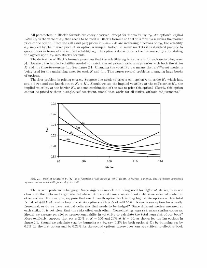
All parameters in Black’s formula are easily observed, except for the volatility ¾B ..An option’s impliedvolatility is the value of ¾B that needs to be used in Black’s formula so that this formula matches the marketprice of the option. Since the call (and put) prices in 2.4a - 2.4c are increasing functions of ¾B , the volatility¾B implied by the market price of an option is unique. Indeed, in many markets it is standard practice toquote prices in terms of the implied volatility ¾B ; the option’s dollar price is then recovered by substitutingthe agreed upon ¾B into Black’s formula.

The derivation of Black’s formula presumes that the volatility ¾B is a constant for each underlying assetA. However, the implied volatility needed to match market prices nearly always varies with both the strikeK and the time-to-exercise tex . See …gure 2.1. Changing the volatility ¾B means that a di¤erent model isbeing used for the underlying asset for each K and tex . This causes several problems managing large booksof options.

The …rst problem is pricing exotics. Suppose one needs to price a call option with strike K1 which has,say, a down-and-out knock-out at K2 < K1. Should we use the implied volatility at the call’s strike K1, theimplied volatility at the barrier K2, or some combination of the two to price this option? Clearly, this optioncannot be priced without a single, self-consistent, model that works for all strikes without “adjustments.”

0.18

0.20

0.22

0.24

0.26

0.28

80 90 100 110 120

Strike

Vol

1m

3m

6m

12m

Fig. 2.1. Implied volatility ¾B(K) as a function of the strike K for 1 month, 3 month, 6 month, and 12 month Europeanoptions on an asset with forward price 100.

The second problem is hedging. Since di¤erent models are being used for di¤erent strikes, it is notclear that the delta and vega risks calculated at one strike are consistent with the same risks calculated atother strikes. For example, suppose that our 1 month option book is long high strike options with a total¢ risk of +$1MM , and is long low strike options with a ¢ of ¡$1MM . Is our is our option book really¢-neutral, or do we have residual delta risk that needs to be hedged? Since di¤erent models are used ateach strike, it is not clear that the risks o¤set each other. Consolidating vega risk raises similar concerns.Should we assume parallel or proportional shifts in volatility to calculate the total vega risk of our book?More explicitly, suppose that ¾B is 20% at K = 100 and 24% at K = 90, as shown for the 1m options in…gure 2.1. Should we calculate vega by bumping ¾B by, say, 0:2% for both options? Or by bumping ¾B by0:2% for the …rst option and by 0:24% for the second option? These questions are critical to e¤ective book

4

management, since this requires consolidating the delta and vega risks of all options on a given asset beforehedging, so that only the net exposure of the book is hedged. Clearly one cannot answer these questionswithout a model that works for all strikes K.

The third problem concerns evolution of the implied volatility curve ¾B(K). Since the implied volatility¾B depends on the strike K, it is likely to also depend on the current value f of the forward price: ¾B =¾B(f ;K ). In this case there would be systematic changes in ¾B as the forward price f of the underlyingchanges See …gure 2.1. Some of the vega risks of Black’s model would actually be due to changes in the priceof the underlying asset, and should be hedged more properly (and cheaply) as delta risks.

2.2. Local volatility models. An apparent solution to these problems is provided by the local volatil-ity model of Dupire [2], which is also attributed to Derman [4], [5]. In an insightful work, Dupire essentiallyargued that Black was to bold in setting the coe¢cient C (t; ¤) to ¾BF . Instead one should only assume thatC is Markovian: C = C(t; F ). Re-writing C(t; F ) as ¾loc(t; F )F then yields the “local volatility model,”where the forward price of the asset is

(2.5a) dF = ¾loc(t; F )F dW; F (0) = f ;

in the forward measure. Dupire argued that instead of theorizing about the unknown local volatility function¾loc(t; F ), one should obtain ¾loc(t; F ) directly from the marketplace by “calibrating” the local volatilitymodel to market prices of liquid European options.

In calibration, one starts with a given local volatility function ¾loc(t; F ), and evaluates

Vcall = D(tset)En[F (tex)¡K]+ jF (0) = f ;

o(2.5b)

´ Vput +D(tset)(f ¡K)(2.5c)

to obtain the theoretical prices of the options; one then varies the local volatility function ¾loc(t; F ) untilthese theoretical prices match the actual market prices of the option for each strike K and exercise datetex . In practice liquid markets usually exist only for options with speci…c exercise dates t1ex; t

2ex ; t

3ex; : : :; for

example, for 1m, 2m, 3m, 6m, and 12m from today. Commonly the local vols ¾loc(t; F ) are taken to bepiecewise constant in time:

¾loc(t; F ) = ¾(1)loc(F ) for t < t1ez ;

¾loc(t; F ) = ¾(j)loc(F ) for tj¡1ex < t < tjez j = 2; 3; :::J(2.6)

¾loc(t; F ) = ¾(J )loc (F ) for t > tJez

One …rst calibrates ¾(1)loc(F ) to reproduce the option prices at t1ex for all strikes K , then calibrates ¾

(2)loc(F ) to

reproduce the option prices at t2ex , for all K, and so forth . This calibration process can be greatly simpli…edby using the results in [13] and [14]. There we solve to obtain the prices of European options under thelocal volatility model 2.5a - 2.5c, and from these prices we obtain explicit algebraic formulas for the impliedvolatility of the local vol models.

Once ¾loc(t; F ) has been obtained by calibration, the local volatility model is a single, self-consistentmodel which correctly reproduces the market prices of calls (and puts) for all strikes K and exercise dates texwithout “adjustment.” Prices of exotic options can now be calculated from this model without ambiguity.This model yields consistent delta and vega risks for all options, so these risks can be consolidated acrossstrikes. Finally, perturbing f and re-calculating the option prices enables one to determine how the impliedvolatilites change with changes in the underlying asset price. Thus, the local volatility model thus providesa method of pricing and hedging options in the presence of market smiles and skews. It is perhaps themost popular method of managing exotic equity and foreign exchange options. Unfortunately, the local

5

volatility model predicts the wrong dynamics of the implied volatility curve, which leads to inaccruate andoften unstable hedges.

To illustrate the problem, consider the special case in which the local vol is a function of F only:

(2.7) dF = ¾loc(F )FdW; F (0) = f:

In [13] and [14] singular perturbation methods were used to analyze this model. There it was found thatEuropean call and put prices are given by Black’s formula 2.4a - 2.4c with the implied volatility

(2.8) ¾B(K; f ) = ¾ loc(12 [f +K])

½1 + 1

24

¾00loc(12[f +K ])

¾loc(12[f +K ])

(f ¡K )2 + ¢ ¢ ¢ :

On the right hand side, the …rst term dominates the solution and the second term provides a much smallercorrection The omitted terms are very small, usually less than 1% of the …rst term.

The behavior of local volatility models can be largely understood by examining the …rst term in 2.8.The implied volatility depends on both the strikeK and the current forward price f: So supppose that todaythe forward price is f0 and the implied volatility curve seen in the marketplace is ¾0B(K). Calibrating themodel to the market clearly requires choosing the local volatility to be

(2.9) ¾loc(F ) = ¾0B(2F ¡ f0)f1 + ¢ ¢ ¢ g:

Now that the model is calibrated, let us examine its predictions. Suppose that the forward value changesfrom f0 to some new value f . From 2.8, 2.9 we see that the model predicts that the new implied volatilitycurve is

(2.10) ¾B(K; f ) = ¾0B(K + f ¡ f0)f1 + ¢ ¢ ¢ g

for an option with strike K, given that the current value of the forward price is f. In particular, if theforward price f0 increases to f , the implied volatility curve moves to the left ; if f0 decreases to f , theimplied volatility curve moves to the right. Local volatility models predict that the market smile/skew movesin the opposite direction as the price of the underlying asset. This is opposite to typical market behavior,in which smiles and skews move in the same direction as the underlying.

To demonstrate the problem concretely, suppose that today’s implied volatility is a perfect smile

(2.11a) ¾0B(K) = ® + ¯[K ¡ f0]2

around today’s forward price f0. Then equation 2.8 implies that the local volatility is

(2.11b) ¾loc(F ) = ®+ 3¯(F ¡ f0)2 + ¢ ¢ ¢ :As the forward price f evolves away from f0 due to normal market ‡uctuations, equation 2.8 predicts thatthe implied volatility is

(2.11c) ¾B(K; f ) = ® + ¯[K ¡ ( 32f0 ¡ 1

2f )]2 + 3

4¯(f ¡ f0)2 + ¢ ¢ ¢ :

. The implied volatility curve not only moves in the opposite direction as the underlying, but the curve alsoshifts upward regardless of whether f increases or decreases. Exact results are illustrated in …gures 2.2 - 2.4.There we assumed that the local volatility ¾loc(F ) was given by 2.11b, and used …nite di¤erence methods toobtain essentially exact values for the option prices, and thus implied volatilites.

Hedges calculated from the local volatility model are wrong. To see this, let BS(f ;K; ¾B ; tex) be Black’sformula 2.4a - 2.4c for, say, a call option. Under the local volatility model, the value of a call option is givenby Black’s formula

(2.12a) Vcall = BS(f;K; ¾B(K; f ); tex)

6

0.18

0.20

0.22

0.24

0.26

0.28

80 90 100 110 120

Impl

ied

Vol

Kf0

Fig. 2.2. Exact implied volatility ¾B(K;f0) (solid line) obtained from the local volatility ¾loc(F ) (dashed line):

0.18

0.20

0.22

0.24

0.26

0.28

80 90 100 110 120

Imp

lied

Vol

Kf0f

Fig. 2.3. Implied volatility ¾B(K;f ) if the forward price decreases from f0 to f (solid line).

with the volatility ¾B(K; f ) given by 2.8. Di¤erentiating with respect to f yields the ¢ risk

(2.12b) ¢ ´ @Vcall@f

=@BS

@f+@BS

@¾B

@¾B(K; f )

@f:

predicted by the local volatility model. The …rst term is clearly the ¢ risk one would calculate from Black’smodel using the implied volatility from the market. The second term is the local volatility model’s correctionto the ¢ risk, which consists of the Black vega risk multiplied by the predicted change in ¾B due to changesin the underlying forward price f . In real markets the implied volatily moves in the opposite direction asthe direction predicted by the model. Therefore, the correction term needed for real markets should havethe opposite sign as the correction predicted by the local volatility model. The original Black model yieldsmore accurate hedges than the local volatility model, even though the local vol model is self-consistent acrossstrikes and Black’s model is inconsistent.

Local volatility models are also peculiar theoretically. Using any function for the local volatility ¾ loc(t; F )except for a power law,

C (t; ¤) = ®(t)F¯ ;(2.13)

¾loc(t; F ) = ®(t)F¯=F = ®(t)=F 1¡¯ ;(2.14)

7

0.18

0.20

0.22

0.24

0.26

0.28

80 90 100 110 120

Impl

ied

Vol

Kf0 f

Fig. 2.4. Implied volatility ¾B(K;f ) if the forward prices increases from f0 to f (solid line).

introduces an intrinsic “length scale” for the forward price F into the model. That is, the model becomesinhomogeneous in the forward price F . Although intrinsic length scales are theoretically possible, it is di¢cultto understand the …nancial origin and meaning of these scales [15], and one naturally wonders whether suchscales should be introduced into a model without speci…c theoretical justi…cation.

2.3. The SABR model. The failure of the local volatility model means that we cannot use a Markov-ian model based on a single Brownian motion to manage our smile risk. Instead of making the modelnon-Markovian, or basing it on non-Brownian motion, we choose to develop a two factor model. To selectthe second factor, we note that most markets experience both relatively quiescent and relatively chaoticperiods. This suggests that volatility is not constant, but is itself a random function of time. Respecting thepreceding discusion, we choose the unknown coe¢cient C (t; ¤) to be ®F ¯ , where the “volatility” ® is itself astochastic process. Choosing the simplest reasonable process for ® now yields the “stochastic-®¯½ model,”which has become known as the SABR model. In this model, the forward price and volatility are

(2.15a) dF = ®F ¯ dW1; F (0) = f

(2.15b) d® = º® dW2; ®(0) = ®

under the forward measure, where the two processes are correlated by:

(2.15c) dW1 dW2 = ½dt:

Many other stochastic volatility models have been proposed, for example [16], [17], [18], [19]; these modelswill be treated in section 5. However, the SABR model has the virtue of being the simplest stochasticvolatility model which is homogenous in F and ®. We shall …nd that the SABR model can be used toaccurately …t the implied volatility curves observed in the marketplace for any single exercise date tex . Moreimportantly, it predicts the correct dynamics of the implied volatility curves. This makes the SABR modelan e¤ective means to manage the smile risk in markets where each asset only has a single exercise date; thesemarkets include the swaption and caplet/‡oorlet markets.

As written, the SABR model may or may not …t the observed volatility surface of an asset which hasEuropean options at several di¤erent exercise dates; such markets include foreign exchange options andmost equity options. Fitting volatility surfaces requires the dynamic SABR model which is introduced andanalyzed in section 4.

8

It has been claimed by many authors that stochastic volatility models are models of incomplete markets,because the stochastic volatility risk cannot be hedged. This is not true. It is true that the risk to changesin ® (the vega risk) cannot be hedged by buying or selling the underlying asset. However, vega risk can behedged by buying or selling options on the asset in exactly the same way that ¢-hedging is used to neutralizethe risks to changes in the price F . In practice, vega risks are hedged by buying and selling options as amatter of routine, so whether the market would be complete if these risks were not hedged is a moot question.

The SABR model 2.15a - 2.15c is analyzed in Appendix B. There singular perturbation techniques areused to obtain the prices of European options. From these prices, the options’ implied volatility ¾B(K; f ) isthen obtained. The upshot of this analysis is that under the SABR model, the price of European options isgiven by Black’s formula,

Vcall = D(tset)ffN (d1)¡KN(d2)g;(2.16a)

Vput = Vcall +D(tset)[K ¡ :f ];(2.16b)

with

(2.16c) d1;2 =log f=K § 1

2¾2Btex

¾Bptex

;

where the implied volatility ¾B(f;K) is given by

¾B(K; f ) =®

(fK )(1¡¯)=2n1 +

(1¡¯)224 log2 f=K +

(1¡¯)41920 log4 f=K + ¢ ¢ ¢

o ¢ µ z

x(z)

¶¢

½1 +

·(1¡¯)224

®2

(fK)1¡¯+ 1

4

½¯º®

(fK )(1¡¯)=2+ 2¡3½2

24º 2¸tex + ¢ ¢ ¢ :(2.17a)

Here

(2.17b) z =º

®(fK )(1¡¯)=2 log f=K;

and x(z) is de…ned by

(2.17c) x(z) = log

(p1 ¡ 2½z + z2 + z ¡ ½

1 ¡ ½

):

For the special case of at-the-money options, options struck at K = f , this formula reduces to

(2.18) ¾ATM = ¾B(f; f ) =®

f (1¡¯)

½1 +

·(1¡¯)224

®2

f 2¡2¯+ 1

4

½¯®º

f (1¡¯)+ 2¡3½2

24º2¸tex + ¢ ¢ ¢ :

These formulas are the main result of this paper. Although it appears formidable, the formula is explicitand only involves elementary trignometric functions. Implementing the SABR model for vanilla options isvery easy, since once this formula is programmed, we just need to send the options to a Black pricer.In thenext section we examine the qualitative behavior of this formula, and how it can be used to managing smilerisk.

The complexity of the formula is needed for accurate pricing. Omitting the last line of 2.17a, for example,can result in a relative error that exceeds three per cent in extreme cases. Although this error term seemssmall, it is large enough to be required for accurate pricing. The omitted terms “+ ¢ ¢ ¢” are much, muchsmaller. Indeed, even though we have derived more accurate expressions by continuing the perturbation

9

expansion to higher order, 2.17a - 2.17c is the formula we use to value and hedge our vanilla swaptions, caps,and ‡oors. We have not implemented the higher order results, believing that the increased precision of thehigher order results is super‡uous.

There are two special cases of note: ¯ = 1, representing a stochastic log normal model), and ¯ = 0,representing a stochastic normal model. The implied volatility for these special cases is obtained in the lastsection of Appendix B.

3. Managing smile risk. The complexity of the above formula for ¾B(K; f ) obscures the qualitativebehavior of the SABR model. To make the model’s phenomenology and dynamics more transparent, notethat formula 2.17a - 2.17c can be approximated as

¾B(K;f ) =®

f 1¡¯©1 ¡ 1

2 (1¡ ¯ ¡ ½¸) logK=f(3.1a)

+ 112

£(1 ¡ ¯ )2 + (2 ¡ 3½2)¸2¤ log2K=f + ¢ ¢ ¢ ;

provided that the strike K is not too far from the current forward f . Here the ratio

(3.1b) ¸ =º

®f 1¡¯

measures the strength º of the volatility of volatility (the “volvol”) compared to the local volatility ®=f 1¡¯

at the current forward. Although equations 3.1a - 3.1b should not be used to price real deals, they areaccurate enough to depict the qualitative behavior of the SABR model faithfully.

As f varies during normal trading, the curve that the ATM volatility ¾B (f; f ) traces is known as thebackbone, while the smile and skew refer to the implied volatility ¾B (K; f ) as a function of strike K fora …xed f. That is, the market smile/skew gives a snapshot of the market prices for di¤erent strikes K ata given instance, when the forward f has a speci…c price. Figures 3.1 and 3.2. show the dynamics of thesmile/skew predicted by the SABR model.

8%

10%

12%

14%

16%

18%

20%

22%

4% 6% 8% 10% 12%

Imp

β = 0

Fig. 3.1. Backbone and smiles for ¯ = 0. As the forward f varies, the implied volatiliity ¾B (f; f ) of ATM optionstraverses the backbone (dashed curve). Shown are the smiles ¾B(K;f ) for three di¤erent values of the forward. Volatility datafrom 1 into 1 swaption on 4/28/00, courtesy of Cantor-Fitzgerald.

Let us now consider the implied volatility ¾B(K;f ) in detail. The …rst factor ®=f 1¡¯ in 3.1a is theimplied volatility for at-the-money (ATM) options, options whose strike K equals the current forward f .So the backbone traversed by ATM options is essentially ¾B(f; f ) = ®=f 1¡¯ for the SABR model. The

10

8%

10%

12%

14%

16%

18%

20%

22%

4% 6% 8% 10% 12%

Impl

ieβ = 1

Fig. 3.2. Backbone and smiles as above, but for ¯ = 1.

backbone is almost entirely determined by the exponent ¯ , with the exponent ¯ = 0 (a stochastic Gaussianmodel) giving a steeply downward sloping backbone, and the exponent ¯ = 1 giving a nearly ‡at backbone.

The second term ¡ 12 (1 ¡ ¯ ¡ ½¸) logK=f represents the skew, the slope of the implied volatility with

respect to the strike K . The ¡ 12 (1 ¡ ¯) logK=f part is the beta skew, which is downward sloping since

0· ¯ · 1. It arises because the “local volatility” ®F ¯=F 1 = ®=F 1¡¯ is a decreasing function of theforward price. The second part 1

2½¸ logK=f is the vanna skew, the skew caused by the correlation between

the volatility and the asset price. Typically the volatility and asset price are negatively correlated, so onaverage, the volatility ® would decrease (increase) when the forward f increases (decreases). It thus seemsunsurprising that a negative correlation ½ causes a downward sloping vanna skew.

It is interesting to compare the skew to the slope of the backbone. As f changes to f 0 the ATM volchanges to

(3.2a) ¾B(f0; f 0) =

®

f 1¡¯f1¡ (1¡ ¯) f

0 ¡ ff

+ ¢ ¢ ¢ g:

Near K = f , the ¯ component of skew expands as

(3.2b) ¾B(K; f ) =®

f 1¡¯f1 ¡ 1

2 (1¡ ¯)K ¡ ff

+ ¢ ¢ ¢ g;

so the slope of the backbone ¾B (f; f ) is twice as steep as the slope of rthe smile ¾B(K; f ) due to the¯-component of the skew.

The last term in 3.1a also contains two parts. The …rst part 112(1 ¡ ¯)2 log2K=f appears to be a smile

(quadratic) term, but it is dominated by the downward sloping beta skew, and, at reasonable strikes K , itjust modi…es this skew somewhat. The second part 1

12(2¡ 3½2)¸2 log2K=f is the smile induced by the volga

(vol-gamma) e¤ect. Physically this smile arises because of “adverse selection”: unusually large movementsof the forward F happen more often when the volatility ® increases, and less often when ® decreases, sostrikes K far from the money represent, on average, high volatility environments.

3.1. Fitting market data. The exponent ¯ and correlation ½ a¤ect the volatility smile in similarways. They both cause a downward sloping skew in ¾B(K; f) as the strike K varies. From a single marketsnapshot of ¾B(K;f ) as a function of K at a given f , it is di¢cult to distinguish between the two parameters.

11

This is demonstrated by …gure 3.3. There we …t the SABR parameters ®; ½; º with ¯ = 0 and then re-…t theparameters ®; ½; º with ¯ = 1. Note that there is no substantial di¤erence in the quality of the …ts, despitethe presence of market noise. This matches our general experience: market smiles can be …t equally wellwith any speci…c value of ¯. In particular, ¯ cannot be determined by …tting a market smile since this wouldclearly amount to “…tting the noise.”

1y into 1y

12%

14%

16%

18%

20%

22%

4% 6% 8% 10% 12%

Impl

ie

Fig. 3.3. Implied volatilities as a function of strike. Shown are the curves obtained by …tting the SABR model withexponent ¯ = 0 and with ¯ =1 to the 1y into 1y swaption vol observed on 4/28/00. As usual, both …ts are equally good. Datacourtesy of Cantor-Fitzgerald.

Figure 3.3 also exhibits a common data quality issue. Options with strikes K away from the currentforward f trade less frequently than at-the-money and near-the-money options. Consequently, as K movesaway from f , the volatility quotes become more suspect because they are more likely to be out-of-date andnot represent bona …de o¤ers to buy or sell options.

Suppose for the moment that the exponent ¯ is known or has been selected. Taking a snapshot of themarket yields the implied volatility ¾B(K; f ) as a function of the strike K at the current forward price f .With ¯ given, …tting the SABR model is a straightforward procedure. The three parameters ®; ½; and ºhave di¤erent e¤ects on the curve: the parameter ® mainly controls the overall height of the curve, changingthe correlation ½ controls the curve’s skew, and changing the vol of vol º controls how much smile the curveexhibits. Because of the widely seperated roles these parameters play, the …tted parameter values tend tobe very stable, even in the presence of large amounts of market noise.

The exponent ¯ can be determined from historical observations of the “backbone” or selected from“aesthetic considerations.” Equation 2.18 shows that the implied volatility of ATM options is

(3.3) log ¾B(f ;f ) = log ®¡ (1¡ ¯ ) log f + log½1 + [ (1¡¯)

2

24

®2

f 2¡2¯+ 1

4

½¯®º

f (1¡¯)+ 2¡3½2

24º 2]tex + ¢ ¢ ¢ :

¾The exponent ¯ can be extracted from a log log plot of historical observations of f; ¾ATM pairs. Since both fand ® are stochastic variables, this …tting procedure can be quite noisy, and as the [¢ ¢ ¢ ]tex term is typicallyless than one or two per cent, it is usually ignored in …tting ¯.

12

Selecting ¯ from “aesthetic” or other a priori considerations usually results in ¯ = 1 (stochastic lognor-mal), ¯ = 0 (stochastic normal), or ¯ = 1

2 (stochastic CIR) models. Proponents of ¯ = 1 cite log normalmodels as being “more natural.” or believe that the horizontal backbone best represents their market. Theseproponents often include desks trading foreign exchange options. Proponents of ¯ = 0 usually believe that anormal model, with its symmetric break-even points, is a more e¤ective tool for managing risks, and wouldclaim that ¯ = 0 is essential for trading markets like Yen interest rates, where the forwards f can be nega-tive or near zero. Proponents of ¯ = 1

2are usually US interest rate desks that have developed trust in CIR

models.It is usually more convenient to use the at-the-money volatility ¾ATM ; ¯; ½; and º as the SABR parame-

ters instead of the original parameters ®,¯; ½; º:The parameter ® is then found whenever needed by inverting2.18 on the ‡y; this inversion is numerically easy since the [¢ ¢ ¢ ]tex term is small. With this parameterization,…tting the SABR model requires …tting ½ and º to the implied volatility curve, with ¾ATM and ¯ given. Inmany markets, the ATM volatilities need to be updated frequently, say once or twice a day, while the smilesand skews need to be updated infrequently, say once or twice a month. With the new parameterization,¾ATM can be updated as often as needed, with ½, º (and ¯) updated only as needed.

Let us apply SABR to options on US dollar interest rates. There are three key groups of Europeanoptions on US rates: Eurodollar future options, caps/‡oors, and European swaptions. Eurodollar futureoptions are exchange-traded options on the 3 month Libor rate; like interest rate futures, EDF options arequoted on 100(1¡ rLibor). Figure 1.1 …ts the SABR model (with ¯ = 1) to the implied volatility for the June99 contracts, and …gures 3.4 - 3.7 …t the model (also with ¯ = 1) to the implied volatility for the September99, December 99, and March 00 contracts. All prices were obtained from Bloomberg Information Serviceson March 23, 1999. Two points are shown for the same strike where there are quotes for both puts and calls.Note that market liquidity dries up for the later contracts, and for strikes that are too far from the money.Consequently, more market noise is seen for these options.

U 9 9 E u r o d o l l a r o p t i o n

1 0

1 5

2 0

2 5

3 0

93.0 94.0 95.0 96.0 97.0S t r i k e

Vol

(%

)

Fig. 3.4. Volatility of the Sep 99 EDF options

Caps and ‡oors are sums of caplets and ‡oorlets; each caplet and ‡oorlet is a European option on the 3month Libor rate. We do not consider the cap/‡oor market here because the broker-quoted cap prices mustbe “stripped” to obtain the caplet volatilities before SABR can be applied.

A m year into n year swaption is a European option with m years to the exercise date (the maturity);if it is exercised, then one receives an n year swap (the tenor, or underlying) on the 3 month Libor rate.See Appendix A. For almost all maturities and tenors, the US swaption market is liquid for at-the-money

13

Z 9 9 E u r o d o l l a r o p t i o n

1 4

1 6

1 8

2 0

92 .0 93 .0 94 .0 95.0 96.0S t r i k e

Vol

(%

)

Fig. 3.5. Volatility of the Dec 99 EDF options

H 0 0 E u r o d o l l a r o p t i o n

1 4

1 6

1 8

2 0

2 2

2 4

92.0 93.0 94 .0 95.0 96 .0 97.0S t r i k e

Vol

(%

)

Fig. 3.6. Volatility of the Mar 00 EDF options

swaptions, but is ill-liquid for swaptions struck away from the money. Hence, market data is somewhatsuspect for swaptions that are not struck near the money. Figures 3.8 - 3.11 …ts the SABR model (with¯ = 1) to the prices of m into5Y swaptions observed on April 28, 2000. Data supplied courtesy of Cantor-Fitzgerald.

We observe that the smile and skew depend heavily on the time-to-exercise for Eurodollar future optionsand swaptions. The smile is pronounced for short-dated options and ‡attens for longer dated options; theskew is overwhelmed by the smile for short-dated options, but is important for long-dated options. Thispicture is con…rmed tables 3.1 and 3.2. These tables show the values of the vol of vol º and correlation ½obtained by …tting the smile and skew of each “m into n” swaption, again using the data from April 28,2000. Note that the vol of vol º is very high for short dated options, and decreases as the time-to-exerciseincreases, while the correlations starts near zero and becomes substantially negative. Also note that thereis little dependence of the market skew/smile on the length of the underlying swap; both º and ½ are fairlyconstant across each row. This matches our general experience: in most markets there is a strong smile for

14

M 0 0 E u r o d o l l a r o p t i o n

1 4

1 6

1 8

2 0

2 2

2 4

92 .0 93.0 94 .0 95.0 96.0 97.0S t r i k e

Vol

(%

)

Fig. 3.7. Volatility of the Jun 00 EDF options

3M into 5Y

12%

14%

16%

18%

20%

4% 6% 8% 10% 12%

Fig. 3.8. Volatilities of 3 month into 5 year swaption

short-dated options which relaxes as the time-to-expiry increases; consequently the volatility of volatility ºis large for short dated options and smaller for long-dated options, regardless of the particular underlying.Our experience with correlations is less clear: in some markets a nearly ‡at skew for short maturity optionsdevelops into a strongly downward sloping skew for longer maturities. In other markets there is a strongdownward skew for all option maturities, and in still other markets the skew is close to zero for all maturities.

3.2. Managing smile risk. After choosing ¯ and …tting ½, º , and either ® or ¾ATM , the SABR model

(3.4a) dF = ®F ¯ dW1; F (0) = f

(3.4b) d® = º® dW2; ®(0) = ®

with

(3.4c) dW1 dW2 = ½dt

15

1Y into 5Y

13%

14%

15%

16%

17%

18%

4% 6% 8% 10% 12%

Fig. 3.9. Volatilities of 1 year into 1 year swaptions

5Y into 5Y

12%

13%

14%

15%

16%

17%

4% 6% 8% 10% 12%

Fig. 3.10. Volatilities of 5 year into 5 year swaptions

…ts the smiles and skews observed in the market quite well, especially considering the quality of price quotesaway from the money . Let us take for granted that it …ts well enough. Then we have a single, self-consistentmodel that …ts the option prices for all strikes K without “adjustment,” so we can use this model to priceexotic options without ambiguity. The SABR model also predicts that whenever the forward price f changes,the the implied volatility curve shifts in the same direction and by the same amount as the price f . Thispredicted dynamics of the smile matches market experience. If ¯ < 1, the “backbone” is downward sloping,so the shift in the implied volatility curve is not purely horizontal. Instead, this curve shifts up and downas the at-the-money point traverses the backbone. Our experience suggests that the parameters ½ and ºare very stable (¯ is assumed to be a given constant), and need to be re-…t only every few weeks. Thisstability may be because the SABR model reproduces the usual dynamics of smiles and skews. In contrast,the at-the-money volatility ¾ATM , or, equivalently, ® may need to be updated every few hours in fast-pacedmarkets.

Since the SABR model is a single self-consistent model for all strikes K, the risks calculated at one strike

16

10Y into 5Y

9%

10%

11%

12%

13%

4% 6% 8% 10% 12%

Fig. 3.11. Volatilities of 10 year into 5 year options

º 1Y 2Y 3Y 4Y 5Y 7Y 10Y1M 76.2% 75.4% 74.6% 74.1% 75.2% 73.7% 74.1%3M 65.1% 62.0% 60.7% 60.1% 62.9% 59.7% 59.5%6M 57.1% 52.6% 51.4% 50.8% 49.4% 50.4% 50.0%1Y 59.8% 49.3% 47.1% 46.7% 46.0% 45.6% 44.7%3Y 42.1% 39.1% 38.4% 38.4% 36.9% 38.0% 37.6%5Y 33.4% 33.2% 33.1% 32.6% 31.3% 32.3% 32.2%7Y 30.2% 29.2% 29.0% 28.2% 26.2% 27.2% 27.0%10Y 26.7% 26.3% 26.0% 25.6% 24.8% 24.7% 24.5%

Table 3.1Volatility of volatility º for European swaptions. Rows are time-to-exercise; columns are tenor of the underlying swap.

are consistent with the risks calculated at other strikes. Therefore the risks of all the options on the sameasset can be added together, and only the residual risk needs to be hedged.

Let us set aside the ¢ risk for the moment, and calculate the other risks. Let BS(f;K; ¾B ; tex) beBlack’s formula 2.4a - 2.4c for, say, a call option. According to the SABR model, the value of a call is

(3.5) Vcall = BS(f;K; ¾B(K; f ); tex)

where the volatility ¾B(K; f ) ´ ¾B(K;f ;®; ¯; ½; º) is given by equations 2.17a - 2.17c. Di¤erentiating1 withrespect to ® yields the vega risk, the risk to overall changes in volatility:

(3.6)@Vcall@®

=@BS

@¾B¢ @¾B(K; f ;®; ¯; ½; º)

@®:

This risk is the change in value when ® changes by a unit amount. It is traditional to scale vega so thatit represents the change in value when the ATM volatility changes by a unit amount. Since ±¾ATM =

1 In practice risks are calculated by …nite di¤erences: valuing the option at ®, re-valuing the option after bumping theforward to ®+ ±, and then subtracting to determine the risk This saves di¤erentiating complex formulas such as 2.17a - 2.17c.

17

½ 1Y 2Y 3Y 4Y 5Y 7Y 10Y1M 4.2% -0.2% -0.7% -1.0% -2.5% -1.8% -2.3%3M 2.5% -4.9% -5.9% -6.5% -6.9% -7.6% -8.5%6M 5.0% -3.6% -4.9% -5.6% -7.1% -7.0% -8.0%1Y -4.4% -8.1% -8.8% -9.3% -9.8% -10.2% -10.9%3Y -7.3% -14.3% -17.1% -17.1% -16.6% -17.9% -18.9%5Y -11.1% -17.3% -18.5% -18.8% -19.0% -20.0% -21.6%7Y -13.7% -22.0% -23.6% -24.0% -25.0% -26.1% -28.7%10Y -14.8% -25.5% -27.7% -29.2% -31.7% -32.3% -33.7%

Table 3.2Matrix of correlations ½ between the underlying and the volatility for European swaptons.

(@¾ATM =@®)±®, the vega risk is

(3.7a) vega ´ @Vcall@®

=@BS

@¾B¢@¾B(K; f ;®; ¯ ;½; º )

@®@¾ATM(f ;®; ¯; ½; º)

@®

where ¾ATM (f ) = ¾B(f; f ) is given by 2.18. Note that to leading order, @¾B=@® ¼ ¾B =® and @¾ATM =@® ¼¾ATM =®, so the vega risk is roughly given by

(3.7b) vega ¼ @BS

@¾B¢ ¾B(K; f )¾ATM (f )

=@BS

@¾B¢ ¾B(K; f )¾B(f; f )

:

Qualitatively, then, vega risks at di¤erent strikes are calculated by bumping the implied volatility at eachstrike K by an amount that is proportional to the implied volatiity ¾B (K; f ) at that strike. That is, inusing equation 3.7a, we are essentially using proportional, and not parallel, shifts of the volatility curve tocalculate the total vega risk of a book of options.

Since ½ and º are determined by …tting the implied volatility curve observed in the marketplace, theSABR model has risks to ½ and º changing. Borrowing terminology from foreign exchange desks, vanna isthe risk to ½ changing and volga (vol gamma) is the risk to º changing:

(3.8a) vanna =@Vcall@½

=@BS

@¾B¢ @¾B(K;f ;®; ¯; ½; º)

@½;

(3.8b) volga =@Vcall

@º=@BS

@¾B¢ @¾B(K; f ;®; ¯; ½; º)

@º:

Vanna basically expresses the risk to the skew increasing, and volga expresses the risk to the smile becomingmore pronounced. These risks are easily calculated by using …nite di¤erences on the formula for ¾B inequations 2.17a - 2.17c. If desired, these risks can be hedged by buying or selling away-from-the-moneyoptions.

The delta risk expressed by the SABR model depends on whether one uses the parameterization ®,¯, ½, º or ¾ATM , ¯, ½, º . Suppose …rst we use the parameterization ®, ¯, ½, º, so that ¾B(K; f ) ´¾B(K; f ;®; ¯; ½; º). Di¤erentiating respect to f yields the ¢ risk

(3.9) ¢ ´ @Vcall

@f=@BS

@f+@BS

@¾B

@¾B(K;f ;®; ¯; ½; º)

@f:

18

The …rst term is the ordinary ¢ risk one would calculate from Black’s model. The second term is the SABRmodel’s correction to the ¢ risk. It consists of the Black vega times the predicted change in the impliedvolatility ¾B caused by the change in the forward f . As discussed above, the predicted change consists ofa sideways movement of the volatility curve in the same direction (and by the same amount) as the changein the forward price f . In addition, if ¯ < 1 the volatility curve rises and falls as the at-the-money pointtraverses up and down the backbone. There may also be minor changes to the shape of the skew/smile dueto changes in f .

Now suppose we use the parameterization ¾AMT , ¯, ½, º. Then ® is a function of ¾ATM and f de…nedimplicitly by 2.18. Di¤erentiating 3.5 now yields the ¢ risk

(3.10) ¢ ´ @BS

@f+@BS

@¾B

½@¾B(K; f ;®;¯ ; ½; º )

@f+@¾B(K; f ;®; ¯; ½; º )

@®

@®(¾ATM ; f )

@f

¾:

The delta risk is now the risk to changes in f with ¾ATM held …xed. The last term is just the change in® needed to keep ¾ATM constant while f changes. Clearly this last term must just cancel out the verticalcomponent of the backbone, leaving only the sideways movement of the implied volatilty curve. Note thatthis term is zero for ¯ = 1.

Theoretically one should use the ¢ from equation 3.9 to risk manage option books. In many markets,however, it may take several days for volatilities ¾B to change following signi…cant changes in the forwardprice f. In these markets, using ¢ from 3.10 is a much more e¤ective hedge. For suppose one used ¢ fromequation 3.9. Then, when the volatility ¾ATM did not immediately change following a change in f , onewould be forced to re-mark ® to compensate, and this re-marking would change the ¢ hedges. As ¾ATMequilibrated over the next few days, one would mark ® back to its original value, which would change the ¢hedges back to their original value. This “hedging chatter” caused by market delays can prove to be costly.

4. The dynamic SABR model. Quote results for smile and skew.For each exercise date, same smile as in the static SABR model! Same smile dynamics!Calibrating volatility surface is no harder than calibrating smile.Show some results. FX options?

5. Conclusions. Other models. Give results for other modelsSABR and dynamic SABR have the advantage of being the simplest models which can be used to

risk-manage smiles/skews.

Appendix A. Martingale pricing.Quote martingale theory. Derive the martingale pricing formulas for general options and for swaptions.

Appendix B. Analysis of the SABR model.Here we use singular perturbation techniques to price European options under the SABR model. Our

analysis is based on a small volatility expansion, where we take both the volatility ® and the “volvol” º to besmall. To carry out this analysis in a systematic fashion, we re-write ® ¡! "®; and º ¡! "º, and analyze

dF = "®C(F )dW1;(B.1a)

d® = "º®dW2;(B.1b)

with

(B.1c) dW1dW2 = ½dt;

in the limit " ¿ 1. This is the distinguished limit [21], [22] in the language of singular perturbation theory.After obtaining the results we replace "® ¡! ®; and "º ¡! º to get the answer in terms of the original

19

variables. We …rst analyze the model with a general C (F ), and then specialize the results to the power lawF¯ . This is notationally simpler than working with the power law throughout, and the more general resultmay prove valuable in some future application.

We …rst use the forward Kolmogorov equation to simplify the option pricing problem. Suppose theeconomy is in state F (t) = f; ®(t) = ® at date t. De…ne the probability density p(t; f; ®; T; F; A) by

(B.2) p(t;f ; ®; T; F; A)dFdA = probnF < F (T ) < F + dF; A < ®(T ) < A + dA

¯F (t) = f; ®(t) = ®

o:

As a function of the forward variables T; F; A; the density p satis…es the forward Kolmogorov equation (theF½okker-Planck equation)

(B.3a) pT =12"2A2[C 2(F )p]FF + "

2½º[A2C(F )p]F A +12"2º 2[A2p]AA for T > t;

with

(B.3b) p = ±(F ¡ f )±(A ¡ ®) at T = t;

as is well-known [24], [25], [26]. Here, and throughout, we use subscripts to denote partial derivatives.Let V (t; f; ®) be the value of a European call option at date t, when the economy is in state F (t) =

f; ®(t) = ®. Let tex be the option’s exercise date, and let K be its strike. Omitting the discount factorD(tset), which factors out exactly, the value of the option is

V (t;f ; ®) = En[F (tex)¡ K]+ j F (t) = f; ®(t) = ®

o(B.4)

=

Z 1

¡1

Z 1

K

(F ¡K )p(t; f ;®; tex; F; A)dF dA:

See 2.1a. Since

(B.5) p(t; f ;®; tex; F; A) = ±(F ¡ f )±(A ¡ ®) +Z tex

t

pT (t;f ; ®; T; F; A)dT;

we can re-write V (t; f; ®) as

(B.6) V (t;f ; ®) = [f ¡K]+ +Z tex

t

Z 1

K

Z 1

¡1(F ¡K)pT (t; f; ®; T; F; A)dAdF dT:

We substitute B.3a for pT into B.6. Integrating the A derivatives "2½º [A2C (F )p]FA and 12"2º2[A2p]AA over

all A yields zero. Therefore our option price reduces to

(B.7) V (t; f; ®) = [f ¡ K]+ + 12"2Z tex

t

Z 1

¡1

Z 1

K

A2 (F ¡ K) [C 2(F )p]FF dFdAdT;

where we have switched the order of integration. Integrating by parts twice with respect to F now yields

(B.8) V (t; f; ®) = [f ¡K]+ + 12 "2C2(K )

Z tex

t

Z 1

¡1A2p(t; f; ®; T;K; A)dAdT:

The problem can be simpli…ed further by de…ning

(B.9) P (t; f; ®; T;K) =

Z 1

¡1A2p(t; f; ®; T;K; A)dA:

20

Then P satis…es the backward’s Kolmogorov equation [24], [25], [26]

Pt +12"2®2C 2(f )Pf f + "

2½º®2C(f )Pf® +12"2º2®2P®® = 0; for t < T(B.10a)

P = ®2±(f ¡K ); for t = T:(B.10b)

Since t does not appear explicitly in this equation, P depends only on the combination T ¡ t, and not on tand T separately. So de…ne

(B.11) ¿ = T ¡ t; ¿ex = tex ¡ t:

Then our pricing formula becomes

(B.12) V (t; f ;®) = [f ¡ K]+ + 12"2C 2(K)

Z ¿ex

0

P (¿; f; ®;K )d¿

where P (¿; f; ®;K) is the solution of the problem

P¿ =12"2®2C2(f )Pff + "

2½º®2C (f )Pf ® +12"2º2®2P®® ; for ¿ > 0;(B.13a)

P = ®2±(f ¡K); for ¿ = 0:(B.13b)

In this appendix we solve B.13a, B.13b to obtain P (¿; f ;®;K), and then substitute this solution into B.12to obtain the option value V (t; f; ®). This yields the option price under the SABR model, but the resultingformulas are awkward and not very useful. To cast the results in a more usable form, we re-compute theoption price under the normal model

(B.14a) dF = ¾NdW;

and then equate the two prices to determine which normal volatility ¾N needs to be used to reproduce theoption’s price under the SABR model. That is, we …nd the “implied normal volatility” of the option underthe SABR model. By doing a second comparison between option prices under the log normal model

(B.14b) dF = ¾BF dW

and the normal model, we then convert the implied normal volatility to the usual implied log-normal (Black-Scholes) volatility. That is, we quote the option price predicted by the SABR model in terms of the option’simplied volatility.

B.1. Singular perturbation expansion. Using a straightforward perturbation expansion would yielda Gaussian density to leading order,

(B.15a) P =®p

2¼"2C2(K)¿e¡ (f¡K)22"2®2C2 (K)¿ f1 + ¢ ¢ ¢ g:

Since the “+ ¢ ¢ ¢ ” involves powers of (f ¡K )="®C (K), this expansion would become inaccurate as soon as(f ¡K )C0(K)=C (K) becomes a signi…cant fraction of 1; i.e., as soon as C(f ) and C (K) are signi…cantlydi¤erent. Stated di¤erently, small changes in the exponent cause much greater changes in the probabilitydensity. A better approach is to re-cast the series as

(B.15b) P =®p

2¼"2C2(K)¿e¡ (f¡K)22"2®2C2 (K)¿ f1+¢¢¢ g

21

and expand the exponent, since one expects that only small changes to the exponent will be needed toe¤ect the much larger changes in the density. This expansion also describes the basic physics better — P isessentially a Gaussian probability density which tails o¤ faster or slower depending on whether the “di¤usioncoe¢cient” C(f ) decreases or increases.

We can re…ne this approach by noting that the exponent is the integral

(B.16)(f ¡K)2

2"2®2C2(K)¿f1 + ¢ ¢ ¢ g = 1

2¿

Ã1

"®

Z f

K

df 0

C(f 0)

!2

f1 + ¢ ¢ ¢ g:

Suppose we de…ne the new variable

(B.17) z =1

"®

Z f

K

df 0

C (f 0):

so that the solution P is essentially e¡z2=2. To leading order, the density is Gaussian in the variable z, which

is determined by how “easy” or “hard” it is to di¤use from K to f , which closely matches the underlyingphysics. The fact that the Gaussian changes by orders of magnitude as z2 increases should be largelyirrelevent to the quality of the expansion. This approach is directly related to the geometric optics techniquethat is so successful in wave propagation and quantum electronics [27], [22]. To be more speci…c, we shalluse the near identity transform method to carry out the geometric optics expansion. This method, pioneeredin [28], transforms the problem order-by-order into a simple canonical problem, which can then be solvedtrivially. Here we obtain the solution only through O("2), truncating all higher order terms.

Let us change variables from f to

(B.18a) z =1

"®

Z f

K

df 0

C (f 0);

and to avoid confusion, we de…ne

(B.18b) B("®z) = C(f):

Then

(B.19a)@

@f¡! 1

"®C (f )

@

@z=

1

"®B("®z)

@

@z;

@

@®¡! @

@®¡ z

®

@

@z;

and

@2

@f 2¡! 1

"2®2B2("®z)

½@2

@z2¡ "® B

0("®z)B("®z)

@

@z

¾;(B.19b)

@2

@f@®¡! 1

"®B("®z)

½@2

@z@®¡ z

®

@2

@z2¡ 1

®

@

@z

¾;(B.19c)

@2

@®2¡! @2

@®2¡ 2z

®

@2

@z@®+z2

®2@2

@z2+2z

®2@

@z:(B.19d)

Also,

(B.19e) ±(f ¡ K) = ±("®zC(K)) = 1

"®C (K)±(z):

22

Therefore, B.12 through B.13b become

(B.20) V (t; f; a) = [f ¡K ]+ + 12"2C2(K)

Z ¿ex

0

P (¿ ; z; ®)d¿;

where P (¿; z; ®) is the solution of

P¿ =12

¡1 ¡ 2"½ºz + "2º2z2¢Pzz ¡ 1

2"aB0

BPz + ("½º ¡ "2º2z)(®Pz® ¡ Pz)(B.21a)

+ 12"2º2®2P®a for ¿ > 0

(B.21b) P =®

"C(K )±(z) at ¿ = 0:

Accordingly, let us de…ne P (¿; z;®) by

(B.22) P ="

®C (K)P:

In terms of P , we obtain

(B.23) V (t; f; a) = [f ¡K]+ + 12 "®C (K)

Z ¿ex

0

P (¿; z;®)d¿ ;

where P (¿; z; ®) is the solution of

P¿ =12

¡1¡ 2"½ºz+ "2º2z2¢ Pzz ¡ 1

2"aB0

BPz + ("½º ¡ "2º2z)®Pz®(B.24a)

+ 12"2º 2(®2P®® + 2®P®) for ¿ > 0;

(B.24b) P = ±(z) at ¿ = 0:

To leading order P is the solution of the standard di¤usion problem P¿ =12 Pzz with P = ±(z) at ¿ = 0.

So it is a Gaussian to leading order. The next stage is to transform the problem to the standard di¤usionproblem through O("), and then through O("2), . . . . This is the near identify transform method which hasproven so powerful in near-Hamiltonian systems [28].

Note that the variable ® does not enter the problem for P until O("), so

(B.25) P (¿; z; ®) = P0(¿; z) + P1(¿; z; ®) + ¢ ¢ ¢Consequently, the derivatives Pz® , P®® , and P® are all O("). Recall that we are only solving for P throughO("2). So, through this order, we can re-write our problem as

P¿ =12

¡1 ¡ 2"½ºz + "2º 2z2¢ Pzz ¡ 1

2"aB 0

BPz + "½º®Pz® for ¿ > 0(B.26a)

P = ±(z) at ¿ = 0:(B.26b)

Let us now eliminate the 12"a(B 0=B)Pz term. De…ne H(¿ ;z; ®) by

(B.27) P =pC(f)=C (K)H ´

pB("®z)=B(0)H:

23

Then

Pz =pB("®z)=B(0)

½Hz +

12 "®

B 0

BH

¾;(B.28a)

Pzz =pB("®z)=B(0)

½Hzz + "®

B 0

BHz + "

2®2·B 00

2B¡ B02

4B2

¸H

¾;(B.28b)

Pz® =pB("®z)=B(0)

½Hz® +

12 "z

B 0

BHz +

12 "®

B 0

BH® +

12 "B0

BH +O("2)

¾:(B.28c)

The option price now becomes

(B.29) V (t; f; a) = [f ¡K]+ + 12"®pB(0)B("®z)

Z ¿ex

0

H (¿; z; ®) d¿ ;

where

H¿ =12

¡1 ¡ 2"½ºz + "2º 2z2¢Hzz¡ 1

2"2½º®

B0

B(zHz ¡H)(B.30a)

+"2®2µ14

B 00

B¡ 3

8

B02

B2

¶H+"½º®(Hz® +

12"®

B 0

BH®) for ¿ > 0

(B.30b) H = ±(z) at ¿ = 0:

Equations B.30a, B.30b are independent of ® to leading order, and at O(") they depend on ® only throughthe last term "½º®(Hz® +

12 "®

B 0B H®). As above, since B.30a is independent of ® to leading order, we can

conclude that the ® derivatives H® and Hz® are no larger than O("), and so the last term is actually nolarger than O("2). Therefore H is independent of ® until O("2) and the ® derivatives are actually no largerthan O("2). Thus, the last term is actually only O("3), and can be neglected since we are only workingthrough O("2). So,

(B.31a) H¿ =12

¡1 ¡ 2"½ºz + "2º 2z2¢Hzz ¡ 1

2"2½º®

B 0

B(zHz ¡H) + "2®2

µ14

B 00

B¡ 3

8

B 02

B2

¶H for ¿ > 0

(B.31b) H = ±(z) at ¿ = 0:

There are no longer any ® derivatives, so we can now treat ® as a parameter instead of as an independentvariable. That is, we have succeeded in e¤ectively reducing the problem to one dimension.

Let us now remove the Hz term through O("2). To leading order, B 0("®z)=B("®z) and B 00("®z)=B("®z)are constant. We can replace these ratios by

(B.32) b1 = B0("®z0)=B("®z0); b2 = B

00("®z0)=B("®z0);

commiting only an O(") error, where the constant z0 will be chosen later. We now de…ne H by

(B.33) H = e"2½º®b1z

2=4H:

Then our option price becomes

(B.34) V (t; f; a) = [f ¡K]+ + 12"®pB(0)B("®z)e"

2½º®b1z2=4

Z ¿ex

0

H(¿ ; z) d¿;

24

where H is the solution of

(B.35a) H¿ =12

¡1¡ 2"½ºz+ "2º2z2¢ Hzz + "

2®2¡14b2 ¡ 3

8b21¢H + 3

4"2½º®b1H for ¿ > 0

(B.35b) H = ±(z) at ¿ = 0:

We’ve almost beaten the equation into shape. We now de…ne

(B.36a) x =1

"º

Z "ºz

0

d³p1 ¡ 2½³ + ³2

=1

"ºlog (

p1 ¡ 2"½ºz + "2º 2z2 ¡ ½+ "ºz

1 ¡ ½ );

which can be written implicitly as

(B.36b) "ºz = sinh"ºx¡ ½(cosh "ºx¡ 1):In terms of x, our problem is

(B.37) V (t; f; a) = [f ¡K ]+ + 12"®pB(0)B("®z)e"

2½º®b1z2=4

Z ¿ex

0

H(¿; x)d¿;

with

(B.38a) H¿ =12 Hxx ¡ 1

2"ºI0("ºz)Hx + "

2®2¡14 b2 ¡ 3

8 b21

¢H + 3

4 "2½º®b1H for ¿ > 0

(B.38b) H = ±(x) at ¿ = 0:

Here

(B.39) I(³) =

q1¡ 2½³ + ³2:

The …nal step is to de…ne Q by

(B.40) H = I1=2("ºz(x))Q =¡1 ¡ 2"½ºz + "2º 2z2¢1=4Q:

Then

Hx = I1=2("ºz)

£Qx +

12"ºI 0("ºz)Q

¤;(B.41a)

Hxx = I1=2("ºz)

£Qxx + "ºI

0Qx + "2º2

¡12 I

00I + 14 I

0I 0¢Q¤;(B.41b)

and so

(B.42) V (t; f; a) = [f ¡ K]+ + 12"®pB(0)B("®z)I1=2("ºz)e

14 "

2½º®b1z2

Z ¿ex

0

Q(¿; x)d¿;

where Q is the solution of

(B.43a) Q¿ =12Qxx + "

2º2¡14 I

00I ¡ 18 I

0I0¢Q + "2®2

¡14 b2 ¡ 3

8 b21

¢Q+ 3

4 "2½º®b1Q

for ¿ > 0, with

(B.43b) Q = ±(x) at ¿ = 0:

25

As above, we can replace I("ºz); I 0("ºz); I 00("ºz) by the constants I("ºz0); I 0("ºz0); I 00("ºz0), and com-mit only O(") errors. De…ne the constant · by

(B.44) · = º2³14I 00("ºz0)I("ºz0)¡ 1

8[I 0("ºz0]

2)´+ ®2

¡14b2 ¡ 3

8b21¢+ 3

4½º®b1;

where z0 will be chosen later. Then through O("2), we can simplify our equation to

Q¿ =12Qxx + "

2·Q for ¿ > 0;(B.45a)

Q = ±(x) at ¿ = 0:(B.45b)

The solution of B.45a, B.45b is clearly

(B.46) Q =1p2¼¿

e¡x2=2¿e"

2·¿ =1p2¼¿

e¡x2=2¿ 1¡

1 ¡ 23·"

2¿ + ¢ ¢ ¢ ¢3=2through O("2).

This solution yields the option price

(B.47) V (t; f; a) = [f ¡K ]+ + 12"®pB(0)B("®z)I1=2("ºz)e

14"

2½º®b1z2

Z ¿ex

0

1p2¼¿

e¡x2=2¿e"

2·¿ d¿:

Observe that this can be written as

(B.48a) V (t; f; a) = [f ¡K]+ + 12

f ¡Kx

Z ¿ex

0

1p2¼¿

e¡x2=2¿ e"

2µe"2·¿ d¿ ;

where

(B.48b) "2µ = log

µ"®z

f ¡KpB(0)B("®z)

¶+ log

µxI1=2("ºz)

z

¶+ 1

4"2½º®b1z

2

Moreover, quite amazingly,

(B.48c) e"2·¿ =

1¡1 ¡ 2

3·"2¿

¢3=2 = 1µ1 ¡ 2"2¿ µ

x2

¶3=2 +O("4);through O("2). This can be shown by expanding "2µ through O("2), and noting that "2µ=x2matches ·=3.Therefore our option price is

(B.49) V (t; f; a) = [f ¡K]+ + 12

f ¡Kx

Z ¿ex

0

1p2¼¿

e¡x2=2¿e"

2µ d¿µ1 ¡ 2¿

x2"2µ

¶3=2 ;and changing integration variables to

(B.50) q =x2

2¿;

reduces this to

(B.51) V (t; f; a) = [f ¡ K]+ + jf ¡Kj4p¼

Z 1

x2

2¿ex

e¡q+"2µ

(q ¡ "2µ)3=2dq:

26

That is, the value of a European call option is given by

(B.52a) V (t; f; a) = [f ¡ K]+ + jf ¡Kj4p¼

Z 1

x2

2¿ex¡ "2µ

e¡q

q3=2dq;

with

(B.52b) "2µ = log

µ"®z

f ¡KpB(0)B("®z)

¶+ log

µxI1=2("ºz)

z

¶+ 1

4 "2½º®b1z

2;

through O("2).

B.2. Equivalent normal volatility. Equations B.52a and B.52a are a formula for the dollar priceof the call option under the SABR model. The utility and beauty of this formula is not overwhelminglyapparent. To obtain a useful formula, we convert this dollar price into the equivalent implied volatilities.We …rst obtain the implied normal volatility, and then the standard log normal (Black) volatility.

Suppose we repeated the above analysis for the ordinary normal model

(B.53a) dF = ¾NdW; F (0) = f :

where the normal volatily ¾N is constant, not stochastic. (This model is also called the absolute or Gaussianmodel). We would …nd that the option value for the normal model is exactly

(B.53b) V (t;f ) = [f ¡K]+ + jf ¡ Kj4p¼

Z 1

(f¡K)22¾2N ¿ex

e¡q

q3=2dq

This can be seen by setting C(f) to 1, setting "® to ¾N and setting º to 0 in B.52a, B.52b. Working outthis integral then yields the exact European option price

(B.54a) V (t; f ) = (f ¡K)N ( f ¡K¾Np¿ ex

) + ¾Np¿ exG( f ¡K

¾Np¿ ex

);

for the normal model, where N is the normal distribution and G is the Gaussian density

(B.54b) G(q) = 1p2¼e¡q

2=2:

From B.53b it is clear that the option price under the normal model matches the option price under theSABR model B.52a, B.52a if and only if we choose the normal volatility ¾N to be

(B.55)1

¾2N=

x2

(f ¡ K)2½1¡ 2"2 µ

x2¿ ex

¾:

Taking the square root now shows the option’s implied normal (absolute) volatility is given by

(B.56) ¾N =f ¡Kx

½1 + "2

µ

x2¿ ex + ¢ ¢ ¢

¾through O("2).

Before continuing to the implied log normal volatility, let us seek the simplest possible way to re-writethis answer which is correct through O("2). Since x = z[1 + O(")], we can re-write the answer as

(B.57a) ¾N =

µf ¡Kz

¶µz

x(z)

¶©1 + "2 (Á1 + Á2 + Á3) ¿ex + ¢ ¢ ¢

ª;

27

where

f ¡Kz

="®(f ¡K)R fK

df 0

C (f 0)

=

Ã1

f ¡KZ f

K

df 0

"®C(f 0)

!¡1

:

This factor represents the average di¢culty in di¤using from today’s forward f to the strike K, and wouldbe present even if the volatility were not stochastic.

The next factor is

(B.57b)z

x(z)=

³

log

Ãp1 ¡ 2½³ + ³2 ¡ ½+ ³

1¡ ½

! ;where

(B.57c) ³ = "ºz =º

®

Z f

K

df 0

C(f 0)=º

®

f ¡KC(fav )

©1 +O("2)

ª:

Here fav =pfK is the geometric average of f and K . (The arithmetic average could have been used equally

well at this order of accuracy). This factor represents the main e¤ect of the stochastic volatility.The coe¢cients Á1, Á2, and Á3 provide relatively minor corrections. Through O("

2) these correctionsare

"2Á1 =1

z2log

µ"®z

f ¡ KpC(f )C (K)

¶=2°2 ¡ °2124

"2®2C2 (fav) + ¢ ¢ ¢(B.57d)

"2Á2 =1

z2log³ xz

£1 ¡ 2"½ºz + "2º2z2¤1=4´ = 2 ¡ 3½2

24"2º 2 + ¢ ¢ ¢(B.57e)

"2Á3 =14"2½®º

B0("ºz0)B("ºz0)

= 14"2½º®°1C (fav ) + ¢ ¢ ¢(B.57f)

where

(B.57g) °1 =C0(fav )C(fav )

; °2 =C00(fav )C (fav)

:

Let us brie‡y summarize before continuing. Under the normal model, the value of a European call optionwith strike K and exercise date ¿ex is given by B.54a, B.54b. For the SABR model,

dF = "®C(F )dW1; F (0) = f(B.58a)

d® = "º ®dW2; ®(0) = ®(B.58b)

(B.58c) dW1dW2 = ½dt;

the value of the call option is given by the same formula, at least through O("2), provided we use the impliednormal volatility

¾N (K) ="®(f ¡K)R fK

df 0

C(f 0)

¢µ

³

x(³)

¶¢(B.59a)

½1 +

·2°2 ¡ °2124

®2C 2 (fav) +14½º®°1C (fav ) +

2¡ 3½224

º 2¸"2¿ ex + ¢ ¢ ¢

¾:

28

Here

(B.59b) fav =pfK; °1 =

C0(fav )C(fav)

; °2 =C00(fav)C (fav)

;

(B.59c) ³ =º

®

f ¡KC (fav )

; x(³) = log

Ãp1 ¡ 2½³ + ³2 ¡ ½ + ³

1¡ ½

!:

The …rst two factors provide the dominant behavior, with the remaining factor 1+[¢ ¢ ¢ ]"2¿ex usually provide-ing corrections of around 1% or so.

One can repeat the analysis for a European put option, or simply use call/put parity. This shows thatthe value of the put option under the SABR model is

(B.60) Vput(f; ®;K) = (K ¡ f )N( K ¡ f¾Np¿ ex

) + ¾Np¿exG( K ¡ f

¾Np¿ ex

)

where the implied normal volatility ¾N is given by the same formulas B.59a - B.59c as the call.We can revert to the original units by replacing "® ¡! ®, "º ¡! º everywhere in the above formulas;

this is equivalent to setting " to 1 everywhere.

B.3. Equivalent Black vol. With the exception of JPY traders, most traders prefer to quote prices interms of Black (log normal) volatilities, rather than normal volatilities. To derive the implied Black volatility,consider Black’s model

(B.61) dF = "¾BF dW; F (0) = f;

where we have written the volatility as "¾B to stay consistent with the preceding analysis. For Black’smodel, the value of a European call with strike K and exercise date ¿ex is

Vcall = fN (d1)¡ KN (d2);(B.62a)

Vput = Vcall +D(tset)[K ¡ f ];(B.62b)

with

(B.62c) d1;2 =log f=K § 1

2"2¾2B¿ ex

"¾Bp¿ ex

;

where we are omitting the overall factor D(tset) as before.We can obtain the implied normal volatility for Black’s model by repeating the preceding analysis for

the SABR model with C(f) = f and º = 0. Setting C (f ) = f and º = 0 in B.59a -B.59c shows that thenormal volatility is

(B.63) ¾N (K) ="¾B(f ¡ K)log f=K

©1¡ 1

24"2¾2B ¿ex + ¢ ¢ ¢

ª:

through O("2). Indeed, in [14] it is shown that the implied normal volatility for Black’s model is

(B.64) ¾N (K) = "¾BpfK

1 + 124log2 f=K + 1

1920log4 f=K + ¢ ¢ ¢

1 + 124

¡1 ¡ 1

120log2 f=K

¢"2¾2B¿ ex +

15760

"4¾4B¿2ex + ¢ ¢ ¢

29

through O("4). We can …nd the implied Black vol for the SABR model by setting ¾N obtained from Black’smodel in equation B.63 equal to ¾N obtained from the SABR model in B.59a - B.59c. Through O("2) thisyields

¾B(K ) =® log f=KR fK

df 0

C(f 0)

¢µ

³

x(³)

¶¢(B.65)

½1 +

·2°2 ¡ °21 + 1=f 2av

24®2C 2 (fav ) +

14½º®°1C (fav) +

2 ¡ 3½224

º 2¸"2¿ex + ¢ ¢ ¢

¾This is the main result of this article. As before, the implied log normal volatility for puts is the same as forcalls, and this formula can be re-cast in terms of the original variables by simpley setting " to 1:

B.4. Stochastic ¯ model. As originally stated, the SABR model consists of the special case C (f ) =f¯ :

dF = "®F¯dW1; F (0) = f(B.66a)

d® = "º ®dW2; ®(0) = ®(B.66b)

(B.66c) dW1dW2 = ½dt:

Making this substitution in ?? - ?? shows that the implied normal volatility for this model is

¾N (K) ="®(1¡ ¯ )(f ¡K)f 1¡¯ ¡K1¡¯ ¢

µ³

x(³)

¶¢(B.67a) ½

1 +

·¡¯ (2¡ ¯)®224f

2¡2¯av

+½®º¯

4f1¡¯av

+2¡ 3½224

º2¸"2¿ ex + ¢ ¢ ¢

¾through O("2), where fav =

pfK as before and

(B.67b) ³ =º

®

f ¡Kf¯av

; x(³) = log

Ãp1¡ 2½³ + ³2 ¡ ½ + ³

1 ¡ ½

!:

We can simplify this formula by expanding

f ¡K =pfK log f=K

©1 + 1

24log2 f=K + 1

1920log4 f=K + ¢ ¢ ¢ ;(B.68a)

f 1¡¯ ¡K1¡¯ = (1 ¡ ¯)(fK )(1¡¯)=2 log f=Kn1 +

(1¡¯)224 log2 f=K +

(1¡¯)41920 log4 f=K + ¢ ¢ ¢(B.68b)

and neglecting terms higher than fourth order. This expansion reduces the implied normal volatility to

¾N (K) = "®(fK)¯=2 1 + 1

24 log2 f=K + 1

1920 log4 f=K + ¢ ¢ ¢

1 + (1¡¯)224

log2 f=K + (1¡¯)41920

log4 f=K + ¢ ¢ ¢¢µ

³

x(³)

¶¢(B.69a) ½

1 +

·¡¯(2 ¡ ¯)®224(fK)1¡¯

+½®º¯

4(fK)(1¡¯)=2+2¡ 3½224

º2¸"2¿ex + ¢ ¢ ¢

¾;

where

(B.69b) ³ =º

®(fK)(1¡¯)=2 log f=K; x(³) = log

Ãp1¡ 2½³ + ³2 ¡ ½ + ³

1 ¡ ½

!:

30

This is the formula we use in pricing European calls and puts.To obtain the implied Black volatility, we equate the implied normal volatility ¾N (K ) for the SABR

model obtained in B.69a - B.69b to the implied normal volatility for Black’s model obtained in B.63. Thisshows that the implied Black volatility for the SABR model is

¾B(K ) ="®

(fK)(1¡¯)=21

1 +(1¡¯)224 log2 f=K +

(1¡¯)41920 log4 f=K + ¢ ¢ ¢

¢µ

³

x(³)

¶¢(B.69c) ½

1 +

·(1 ¡ ¯)2®224(fK)1¡¯

+½®º¯

4(fK)(1¡¯)=2+2¡ 3½224

º2¸"2¿ex + ¢ ¢ ¢

¾;

through O("2), where ³ and x(³) are given by B.69b as before. Apart from setting " to 1 to recover theoriginal units, this is the formula quoted in section 2, and …tted to the market in section 3.

B.5. Special cases. Two special cases are worthy of special treatment: the stochastic normal model(¯ = 0) and the stochastic log normal model (¯ = 1). Both these models are simple enough that theexpansion can be continued through O("4). For the stochastic normal model (¯ = 0) the implied volatilitiesof European calls and puts are

(B.70a) ¾N (K) = "®

½1 +

2¡ 3½224

"2º2¿ex + ¢ ¢ ¢¾

(B.70b) ¾B(K ) = "®log f=K

f ¡K ¢µ

³

x(³)

¶¢½1 +

·®2

24fK+2 ¡ 3½224

º 2¸"2¿ex + ¢ ¢ ¢

¾through O("4), where

(B.70c) ³ =º

®

pfK log f=K; x(³) = log

Ãp1 ¡ 2½³ + ³2¡ ½ + ³

1 ¡ ½

!:

For the stochastic log normal model (¯ = 1) the implied volatilities are

(B.71a) ¾N (K) = "®f ¡Klog f=K

¢µ

³

x(³)

¶¢ ©1 + £¡ 1

24®2+ 1

4½®º +124 (2 ¡ 3½2)º2

¤"2¿ex + ¢ ¢ ¢

ª

(B.71b) ¾B(K) = "® ¢µ

³

x(³)

¶¢ ©1 + £ 1

4½®º + 1

24(2 ¡ 3½2)º2¤ "2¿ex + ¢ ¢ ¢ ª

through O("4), where

(B.71c) ³ =º

®log f=K; x(³) = log

Ãp1¡ 2½³ + ³2 ¡ ½ + ³

1 ¡ ½

!:

Appendix C. Analysis of the dynamic SABR model.We use e¤ective medium theory [23] to extend the preceding analysis to the dynamic SABR model. As

before, we take the volatility °(t)® and “volvol” º(t) to be small, writng °(t) ¡! "°(t); and º (t)¡! "º(t),and analyze

dF = "°(t)®C(F )dW1;(C.1a)

d® = "º(t)®dW2;(C.1b)

31

with

(C.1c) dW1dW2 = ½(t)dt;

in the limit " ¿ 1. We obtain the prices of European options, and from these prices we obtain the impliedvolatity of these options. After obtaining the results, we replace "°(t) ¡! °(t) and "º(t) ¡! º (t) to get theanswer in terms of the original variables.

Suppose the economy is in state F (t) = f; ®(t) = ® at date t. Let V (t; f ;®) be the value of, say, a Euro-pean call option with strike K and exercise date tex . As before, de…ne the transition density p(t; f; ®; T; F; A)by

(C.2a) p(t; f; ®; T; F; A)dFdA ´ probnF < F (T) < F + dF; A < ®(T ) < A + dA

¯F (t) = f ; ®(t) = ®

oand de…ne

(C.2b) P (t; f; ®; T;K) =

Z 1

¡1A2p(t; f; ®; T;K; A)dA:

Repeating the analysis in Appendix B through equation B.10a, B.10b now shows that the option price isgiven by

(C.3) V (t; f; a) = [f ¡K ]+ + 12"2C2(K)

Z tex

t

°2(T)P (t; f; ®; T;K) dT;

where P (t; f; ®; T;K) is the solution of the backwards problem

Pt +12"2©°2®2C 2(f )Pff + 2½°º®

2C(f)Pf® + º2®2P®®

ª= 0; for t < T(C.4a)

P = ®2±(f ¡ K); for t = T:(C.4b)

We eliminate °(t) by de…ning the new time variable

(C.5) s =

Z t

0

°2(t0)dt0; s 0 =Z T

0

°2(t0)dt0; sex =

Z tex

0

°2(t0)dt0:

Then the option price becomes

(C.6) V (t; f; a) = [f ¡K]+ + 12"2C2(K)

Z sex

s

P (s; f; ®; s0; K )ds0;

where P (s; f; ®; s0;K ) solves the forward problem

Ps +12"2©®2C 2(f )Pff + 2´(s)®

2C(f )Pf® + À2(s)®2P®®

ª= 0 for s < s0(C.7a)

P = ®2±(f ¡ K); for s = s0:(C.7b)

Here

(C.8) ´(s) = ½(t)º(t)=°(t); À(s) = º(t)=°(t):

We solve this problem by using an e¤ective media strategy [23]. In this strategy our objective is todetermine which constant values ¹ and ¹À yield the same option price as the the time dependent coe¢cients´(s) and À(s). If we could …nd these constant values, this would reduce the problem to the non-dynamicSABR model solved in Appendix B.

32

We carry out this strategy by applying the same series of time-independent transformations that wasused to solve the non-dynamic SABR model in Appendix B, de…ning the transformations in terms of the(as yet unknown) constants ¹ and ¹À. The resulting problem is relatively complex, more complex than thecanonical problem obtained in Appedix B. We use a regular perturbation expansion to solve this problem,and once we have solved this problem, we choose ¹ and ¹À so that all terms arising from the time dependenceof ´(t) and À(t) cancel out. As we shall see, this simultaneously determines the “e¤ective” parameters andallows us to use the analysis in Appendix B to obtain the implied volatility of the option.

C.1. Transformation. As in Appendix B, we change independent variables to

(C.9a) z =1

"®

Z f

K

df 0

C (f 0);

and de…ne

(C.9b) B("®z) = C(f):

We then change dependent variables from P to P , and then to H :

(C.9c) P ="

®C (K)P;

(C.9d) H =pC (K)=C(f )P ´

pB(0)=B("®z)P :

Following the reasoning in Appendix B, we obtain

(C.10) V (t; f; a) = [f ¡ K]+ + 12 "®

pB(0)B("®z)

Z sex

s

H(s; z; ®; s0)ds0;

where H (s; z;®; s0) is the solution of

(C.11a) Hs +12

¡1¡ 2"´z + "2À2z2¢Hzz ¡ 1

2"2´®

B 0

B(zHz ¡H) + "2®2

µ14

B 00

B¡ 3

8

B 02

B2

¶H = 0

for s < s0, and

(C.11b) H = ±(z) at s = s0

through O("2). See B.29, B.31a, and B.31b. There are no ® derivatives in equations C.11a, C.11b, so we cantreat ® as a parameter instead of a variable. Through O("2) we can also treat B 0=B and B 00=B as constants:

(C.12) b1 ´ B 0("®z0)B("®z0)

; b2 ´ B 00("®z0)B("®z0)

;

where z0 will be chosen later. Thus we must solve

(C.13a) Hs +12

¡1 ¡ 2"´z + "2À2z2¢Hzz ¡ 1

2 "2´®b1(zHz ¡H) + "2®2

¡14 b2¡ 3

8 b21

¢H = 0 for s < s 0;

(C.13b) H = ±(z) at s = s0:

33

At this point we would like to use a time-independent transformation to remove the zHz term fromequation C.13a. It is not possible to cancel this term exactly, since the coe¢cient ´(s) is time dependent.Instead we use the transformation

(C.14) H = e14"

2®b1±z2

H ,

where the constant ± will be chosen later. This transformation yields

Hs +12

¡1¡ 2"´z+ "2À2z2¢ Hzz ¡ 1

2"2®b1(´ ¡ ±)zHz

+ 14 "2®b1(2´ + ±)H + "2®2

¡14b2 ¡ 3

8 b21

¢H = 0 for s < s0;

(C.15b) H = ±(z) at s = s0;

through O("2). Later the constant ± will be selected so that the change in the option price caused by theterm 1

2 "2®b1´zHz is exactly o¤set by the change in price due to 1

2 "2®b1±zHz term. In this way to the

transformation cancels out the zHz term “on average.”In a similar vein we de…ne

(C.16a) I("¹Àz) =p1 ¡ 2"¹z + "2¹À2z2;

and

(C.16b) x =1

"¹À

Z "¹Àz

0

d³

I(³)=1

"¹Àlog (

p1¡ 2"¹z+ "2¹À2z2 ¡ ¹=¹À + "¹Àz

1 ¡ ¹=¹À );

where the constants ¹ and ¹À will be chosen later. This yields

(C.17a) Hs +12

1¡ 2"´z + "2À2z21¡ 2"¹z + "2¹À2z2 (Hxx ¡ "¹ÀI0("¹Àz)Hx)¡ 1

2"2®b1(´ ¡ ±)xHx

+ 14"2®b1(2´ + ±)H + "2®2

¡14b2 ¡ 3

8b21¢H = 0 for s < s0;

(C.17b) H = ±(x) at s = s0;

through O("2). Here we used z = x + ¢ ¢ ¢ and zHz = xHx + ¢ ¢ ¢ to leading order to simplify the results.Finally, we de…ne

(C.18) H = I1=2("¹Àz)Q:

Then the price of our call option is

(C.19) V (t; f; a) = [f ¡K ]+ + 12"®pB(0)B("®z)I1=2("¹Àz)e

14 "

2®b1±z2

Z sex

s

Q(s; x; s0)ds 0;

where Q(s; x; s0) is the solution of

(C.20a) Qs +12

1¡ 2"´z + "2À2z21¡ 2"¹z + "2¹À2z2Qxx ¡ 1

2"2®b1(´ ¡ ±)xQx +

14"2®b1(2´ + ±)Q

34

+"2¹À2¡14 I

00I ¡ 18 I0I 0¢Q+ "2®2

¡14 b2 ¡ 3

8 b21

¢Q = 0 for s < s0;

(C.20b) Q = ±(x) at s = s0;

Using

(C.21) z = x¡ 12"¹x2 + ¢ ¢ ¢ ;

we can simplify this to

(C.22a) Qs +12Qxx = "(´ ¡ ¹)xQxx ¡ 1

2"2£À2 ¡ ¹À2¡ 3¹(´ ¡ ¹)¤ x2Qxx +

12"2®b1(´ ¡ ±)(xQx ¡Q)

¡ 34"2®b1±Q ¡ "2¹À2

¡14I0 0I ¡ 1

8I 0I 0

¢Q ¡ "2®2 ¡ 1

4b2 ¡ 3

8b21¢Q for s < s0;

(C.22b) Q = ±(x) at s = s0;

through O("2). Note that I; I 0; and I 00 can be replaced by the constants I("¹Àz0); I0("¹Àz0), and I 00("¹Àz0)through O("2).

C.2. Perturbation expansion. Suppose we were to expand Q(s; x; s0) as a power series in " :

(C.23) Q(s; x; s0) = Q(0)(s; x; s0) + "Q(1)(s; x; s 0) + "2Q(2)(s; x;s 0) + ¢ ¢ ¢ :

Substituting this expansion into C.22a, C.22b yields the following hierarchy of equations. To leading orderwe have

Q(0)s + 12Q

(0)xx = 0 for s < s0;(C.24a)

Q(0) = ±(x) at s = s0:(C.24b)

At O(") we have

(C.25a) Q(1)s + 1

2Q(1)xx = (´ ¡ ¹)xQ(0)xx for s < s0;

(C.25b) Q(1) = 0 at s = s0:

At O("2) we can break the solution into

(C.26) Q(2) = Q(2s) +Q(2a) +Q(2b);

where

(C.27a) Q(2s)s + 12Q(2s)xx = ¡ 3

4ab1±Q

(0)¡ ¹À2 ¡14I 00I ¡ 1

8I 0I 0

¢Q(0) ¡ ®2 ¡1

4b2 ¡ 3

8b21¢Q(0) for s < s0;

(C.27b) Q(2s) = 0 at s = s0;

where

(C.28a) Q(2a)s + 12Q(2a)xx = 1

2®b1(´ ¡ ±)(xQ(0)x ¡Q(0)) for s < s0;

35

(C.28b) Q(2a) = 0 at s = s0;

and where

(C.29a) Q(2b)s + 1

2Q(2b)xx = (´ ¡ ¹)xQ(1)xx ¡ 1

2

£À2¡ ¹À2 ¡ 3¹(´ ¡ ¹)¤ x2Q(0)

xx for s < s0;

(C.29b) Q(2b) = 0 at s = s 0:

Once we have solved these equations, then the option price is then given by

(C.30a) V (t; f; a) = [f ¡ K]+ + 12"®pB(0)B("®z)I1=2("z)e

14"

2ab1±z2

J;

where

J =

Z sex

s

Q(0)(s; x; s 0) ds0 + "Z sex

s

Q(1)(s; x; s 0) ds0 + "2Z sex

s

Q(2s)(s; x; s 0) ds0(C.30b)

+"2Z sex

s

Q(2a)(s; x;s 0) ds0 + "2Z sex

s

Q(2b)(s; x; s0)ds 0 + ¢ ¢ ¢ :

The termsQ(1); Q(2a); and Q(2b) arise from the time-dependence of the coe¢cients ´(s) and À(s). Indeed,if ´(s) and À(s) were constant in time, we would have Q(1) ´ Q(2a) ´ Q(2b) ´ 0, and the solution would bejust Q(s) ´ Q(0) + "2Q(2s). Therefore, we will …rst solve for Q(1); Q(2a); and Q(2b), and then try to choosethe constants ± , ¹; and ¹À so that the last three integrals are zero for all x. In this case, the option pricewoud be given by

(C.31a) V (t; f; a) = [f ¡K ]+ + 12 "®

pB(0)B("®z)I1=2("z)e

14"

2ab1±z2Z sex

s

Q(s)(s; x; s0)ds0;

and, through O("2), Q(s) would be the solution of the static problem

(C.31b) Q(s)s + 12Q(s)xx = ¡ 3

4"2ab1±Q

(s) ¡ "2¹À2 ¡14I 00I ¡ 1

8I 0I 0

¢Q(s) ¡ "2®2 ¡1

4b2 ¡ 3

8b21¢Q(s) for s < s0;

(C.31c) Q(s) = ±(x) at s = s0:

This is exactly the time-independent problem solved in Appendix B. See equations B.42, B.43a, and B.43b.So if we can carry out this strategy, we can obtain option prices for the dynamic SABR model by reducingthem to the previously-obtained prices for the static model.

C.2.1. Leading order analysis. The solution of C.24a, C.24b is Gaussian:

(C.32a) Q(0) = G(x=p¢)

where

(C.32b) G(x=p¢) =

1p2¼¢

e¡x2=2¢ ; ¢ = s0 ¡ s:

For future reference, note that

Gx = ¡ x¢G; Gxx =

x2 ¡¢¢2

G; Gxxx = ¡x3¡ 3¢x¢3

G;(C.33a)

Gxxxx =x4 ¡ 6¢x2 + 3¢2

¢4G; Gxxxxx = ¡x

5 ¡ 10¢x3 + 15¢2x

¢5G;(C.33b)

Gxxxxxx =x6 ¡ 15¢x4 + 45¢2x2 ¡ 15¢3

¢6G:(C.33c)

36

C.2.2. Order ". Substituting Q(0) into the equation for Q(1) and using C.33a yields

Q(1)s + 12Q

(1)xx = (´ ¡ ¹)

x3 ¡¢x¢2

G(C.34)

= ¡(s 0 ¡ s)(´ ¡ ¹)Gxxx ¡ 2(´ ¡ ¹)Gx for s < s 0;

with the “initial” condition Q(1) = 0 at s = s0. The solution is

Q(1) = A(s; s0)Gxxx + 2As0(s; s 0)Gx(C.35a)

=@

@s0

n2A(s; s0)Gx(x=

ps0 ¡ s

o;(C.35b)

where

(C.35c) A(s; s0) =Z s0

s

(s0 ¡ ~s)[´(~s)¡ ¹]d~s; As0(s; s0) =

Z s0

s

[´(~s)¡ ¹]d~s:

This term contributes

(C.36)Z sex

s

Q(1)(s; x; s0)ds0 = 2A(s; sex)Gx(x=psex ¡ s)

to the option price. See equations C.30a, C.30b. To eliminate this contribution, we chose ¹ so that A(s; sex) =0:

(C.37) ¹ =

R sexs (sex ¡ ~s)´(~s)d~s

12(sex ¡ s)2

:

C.2.3. The "2Q(2a) term. From equation C.28a we obtain

Q(2a)s + 1

2Q(2a)xx = ¡ 1

2®b1(´ ¡ ±)x

2 +¢

¢G(C.38)

= ¡ 12®b1(´ ¡ ±)¢Gxx ¡ ®b1(´ ¡ ±)G

for s < s0, with Q(2a) = 0 at s = s0. Solving then yields

(C.39) Q(2a) =@

@s0

(®b1

Z s0

s

(s0 ¡ ~s)[´(~s)¡ ± ]d~s G(x=ps0 ¡ s)):

This term makes a contribution of

(C.40)

Z sex

s

Q(2a)(s; x; s0)ds0 = ®b1

µZ sex

s

(sex ¡ ~s)[´(~s)¡ ± ]d~s¶G(x=

psex ¡ s)

to the option price, so we choose

(C.41) ± = ¹ =

R sexs(sex ¡ ~s)[´(~s)¡ ±]d~s

12(sex ¡ ~s)2

:

to eliminate this contribution.

37

C.2.4. The "2Q(2b) term. Substituting Q(1) and Q(0) into equation C.29a, we obtain

(C.42a) Q(2b)s + 1

2Q(2b)xx = (´ ¡ ¹)AxGxxxxx + 2(´ ¡ ¹)As0xGxxx ¡ 1

2·x2Gxx ;

for s < s0, where

(C.42b) · = À2(s)¡ ¹À2 ¡ 3¹[ (s)¡ ¹]:This can be re-written as

Q(2b)s + 12Q

(2b)xx = ¡(´ ¡ ¹)A[¢Gxxxxxx + 5Gxxxx ] ¡ 2(´ ¡ ¹)As0 [¢Gxxxx + 3Gxx ](C.43)

¡ 12·[¢2Gxxxx + 5¢Gxx + 2G]

Solving this with the initial condition Q(2b) = 0 at s = s0 yields

Q(2b) = 12A

2(s; s0)Gxxxxxx + 2A(s; s0)As0(s; s

0)Gxxxx(C.44)

¡3Z s0

s

[´(~s)¡ ¹]A(~s;s 0)d~sGxxxx + 3A2s0(s; s0)Gxx

+ 12

Z s0

s

[s 0 ¡ ~s]2·(~s)d~sGxxxx +52

Z s 0

s

[s 0 ¡ ~s]·(~s)d~sGxx +

Z s0

s

·(~s)d~s G:

This can be written as

Q(2b) =@

@s0

(4A2(s; s0)Gss + 12

Z s 0

s

[ (~s)¡ ¹]A(~s; s 0)d~s Gs(C.45)

¡2Z s0

s

(s 0 ¡ ~s)2·(~s)d~sGs +

Z s0

s

(s0 ¡ ~s)·(~s)d~s G)

Recall that ¹ was chosen above so that A(s; sex) = 0. Therefore the contribution of Q(2b) to the option priceis Z sex

s

Q(2b)(s; x; s 0)ds 0 =µ12

Z sex

s

[ (~s)¡ ¹]A(~s; sex)d~s ¡ 2Z sex

s

(sex ¡ ~s)2·(~s)d~s¶Gs(x=

psex ¡ s)(C.46)

+

µZ sex

s

(sex ¡ ~s)·(~s)d~s¶G(x=

psex ¡ s);

where · = À2(s)¡ ¹À2 ¡ 3¹[ (s)¡ ¹].We can choose the remaining “e¤ective media” parameter ¹À to set either the coe¢cient ofGs(x=

psex ¡ s)

or the coe¢cient of G(x=psex ¡ s) to zero, but cannot set both to zero to completely eliminate the contri-

bution of the term Q(2b). We choose ¹À to set the coe¢cient of Gs(x=psex ¡ s) to zero, for reasons that will

become apparent in a moment:

¹À2 =1

13 (sex ¡ ~s)3

½Z sex

s

(sex ¡ ~s)2À2(~s)d~s ¡ 3¹Z sex

s

(sex ¡ ~s)2[´(~s)¡ ¹]d~s(C.47)

+6

Z sex

s

Z s1

s

s2[´(s1) ¡ ¹][ (s2)¡ ¹]ds2ds1:

Then the remaining contribution to the option price is

(C.48a)Z sex

s

Q(2b)(s; x;s 0)ds 0 = 12¹·(sex ¡ s)2G(x=

psex ¡ s);

38

where

(C.48b) ¹· =1

12 (sex ¡ s)2

Z sex

s

(sex ¡ ~s)[À2(~s)¡ ¹À2]d~s:

Here we have used SinceR sexs (sex ¡ ~s)(´ (~s)¡ ¹)d~s = 0 to simplify C.48b.

C.3. Equivalent volatilities. Let us gather the results together. The static problem C.31b - C.31cis homogeneous in time, so its solution Q(s) depends only on the time di¤erence ¿ ¡ ¿ 0. The option price isthus

(C.49) V (t; f; a) = [f ¡K]+ + 12"®pB(0)B("®z)I1=2("z)e

14"

2ab1¹z2

½Z ¿

0

Qs(~¿; x)d~¿ + 12"2¿2¹µ G(x=

p¿)

¾;

where Qs(¿; x) is the solution of

(C.50a) Qs¿ ¡ 12Q

sxx =

34 "2ab1¹Q

s + "2¹À2¡14 I

00I ¡ 18I0I 0¢Qs + "2®2

¡14 b2 ¡ 3

8 b21

¢Qs for ¿ > 0;

(C.50b) Qs = ±(x) at ¿ = 0:

Here we have replaced ± with ¹. See C.41.Since the static solution is Gaussian to leading order, Qs =G (x=

p¿), we can re-write the option price as

(C.51a) V (t; f; a) = [f ¡ K]+ + 12"®pB(0)B("®z)I1=2("¹Àz)e

14"

2ab1 ¹z2

Z ¿ex

0

Qs(~¿; x)d~¿

through O("2), where

(C.51b) ¿ex = ¿ + 12"2¿2¹µ:

The partial di¤erential equation C.50a, C.50b, and option price C.51a are identical to the equations obtainedin Appendix B for the original non-dynamic SABR model, provided we make the identi…cations

¿ex = ¿ + "2Z ¿

0

~¿ [À2(~¿)¡ ¹À2]d~¿;(C.52a)

º ! ¹=¹À; º ! ¹À:(C.52b)

See equations B.42 - B.43b. Following the reasoning in the preceding Appendix now shows that the Europeancall price is given by the formula

(C.53) V (t; f; K ) = (f ¡ K)N ( f ¡K¾Np¿ex

) + ¾Np¿ exG( f ¡ K

¾Np¿ex

);

with the implied normal volatility

¾N (K ) ="®(f ¡K)R fK

df 0

C(f 0)

¢µ

³

x(³)

¶¢(C.54a)

½1 +

·2°2 ¡ °2124

®2C 2 (fav) +14 ¹®°1C (fav) +

2¹À2 ¡ 3¹224

+ 12¹µ

¸"2¿ ex + ¢ ¢ ¢ :

39

where

(C.54b) ³ =¹À

®

f ¡KC(fav)

; x(³) = log

0@q1¡ 2¹³=¹À+ ³2 ¡ ¹=¹À + ³

1 ¡ ¹=¹À

1A ;

(C.54c) fav =pfK; °1 =

C0(fav )C(fav)

; °2 =C00(fav)C (fav)

;

(C.54d) ¹µ =

R ¿0~¿ [À2(~¿)¡ ¹À2]d~¿

12¿2

:

Equivalently, the option prices are given by Black’s formula with the e¤ective Black volatility of

¾B(K) =® log f=KR fK

df 0

C (f 0)

¢µ

³

x(³)

¶¢(C.55)

½1 +

·2°2 ¡ °21 + 1=f 2av

24®2C2 (fav) +

14 ¹®°1C (fav) +

2¹À2 ¡ 3¹224

+ 12¹µ

¸"2¿ex + ¢ ¢ ¢

Appendix D. Analysis of other stochastic vol models.Adapt analysis to other SV models. Just quote results?

Appendix E. Analysis of other stochastic vol models.Adapt analysis to other SV models. Just quote results?

REFERENCES

[1] D. T. Breeden and R. H. Litzenberger, Prices of state-contingent claims implicit in option prices, J. Business, 51(1994), pp. 621-651.

[2] Bruno Dupire, Pricing with a smile, Risk, Jan. 1994, pp. 18–20.[3] Bruno Dupire, Pricing and hedging with smiles, in Mathematics of Derivative Securities, M.A. H. Dempster and S. R.

Pliska, eds., Cambridge University Press, Cambridge, 1997, pp. 103–111[4] E. DermaN and I. Kani, Riding on a smile, Risk, Feb. 1994, pp. 32–39.[5] E. Derman and I. Kani, Stochastic implied trees: Arbitrage pricing with stochastic term and strike structure of volatility,

Int J. Theor Appl Finance, 1 (1998), pp. 61–110.[6] Harrison and Pliska, Martingale pricing, SIAM J. Abbrev. Correctly, 2 (1992), pp. 000–000.[7] El Karoui & friends, Martingale pricing in incomplete markets, SIAM J. Abbrev. Correctly, 2 (1992), pp. 000–000.[8] Oxendall, Martingale pricing in incomplete markets, SIAM J. Abbrev. Correctly, 2 (1992), pp. 000–000.[9] Jamshidean, Jamshidean uses level numeraire, SIAM J. Abbrev. Correctly, 2 (1992), pp. 000–000.[10] Fischer Black, Black’s model 1, SIAM J. Abbrev. Correctly, 2 (1992), pp. 000–000.[11] John C. Hull, A Beginner’s Book of Option Pricing, Springer-Verlag, Berlin, New York, 1991.[12] Paul X Wilmott, Another Beginner’s Book of Option Pricing, Springer-Verlag, Berlin, New York, 1991[13] Patrick S. Hagan and Diana E. Woodward, Equivalent Black volatilities, App. Math. Finance, 6 (1999), pp. 147–157[14] P. S. Hagan, A. Lesniewski and D. E. Woodward, Geometric optics, App. Math. Finance, 6 (1999), pp. 147–157[15] Fred Wan, A Beginner’s Book of Modeling, Springer-Verlag, Berlin, New York, 1991.[16] Hull and White, Stochastic vol models, App. Math. Finance, 6 (1987), pp. 147–157[17] Heston, Stochactic vol models, App. Math. Finance, 6 (1999), pp. 147–157[18] Someone else, Stochactic vol models, App. Math. Finance, 6 (1999), pp. 147–157[19] Someone else, Stochactic vol models, App. Math. Finance, 6 (1999), pp. 147–157[20] Paribas option guy, Vanna & volga, App. Math. Finance, 6 (1999), pp. 147–157[21] J. D. Cole, Perturbation Theory, Springer-Verlag, Berlin, New York, 1991.

40

[22] J. Kevorkian and J. D. Cole, Perturbation Theory, Springer-Verlag, Berlin, New York, 1991.[23] Andrew Norris, E¤ective medium theory, SIAM J Appl Math, 6 (1999), pp. 147–157[24] Math Guy A, Stochastic Processes A, Springer-Verlag, Berlin, New York, 1991[25] Math Guy B, Stochastic Processes B, Springer-Verlag, Berlin, New York, 1991[26] Math Guy C, Stochastic Processes C, Springer-Verlag, Berlin, New York, 1991[27] G. B. Whitham, Linear and Nonlinear Waves, Springer-Verlag, Berlin, New York, 1991[28] John C. Neu, Thesis, Springer-Verlag, Berlin, New York, 1991

41