Kevin Savage

Toilet Stats

Measuring usage

• This talk is about measuing usage• What we measure• How we use R to predict future usage• Specific code examples• Things that didn't work for us

Background

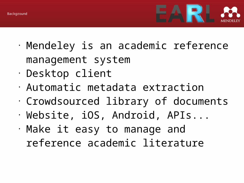
• Mendeley is an academic reference management system

• Desktop client• Automatic metadata extraction• Crowdsourced library of documents• Website, iOS, Android, APIs...• Make it easy to manage and reference

academic literature

Background

• Mendeley bought in 2013 by the publisher Elsevier

• Up until then we used burn rate• Our targets were changed to growth• Measured in quite a complicated way

Burn rate

• As a start-up you have funding from investers and income from customers

• You have to make a profit before you "burn" all your investment money

• If you don't, the business fails• You measure your "burn rate"

Core Users

Core Users = Measured Core Users + Estimated Core Users

Core Users

Core Users = Measured Core Users + Estimated Core Users

MCU if > X sessions in the past 24 weeks

Core Users

Core Users = Measured Core Users + Estimated Core Users

MCU if > X sessions in the past 24 weeks

ECU if > Y sessions in the second week and they are <24 weeks old

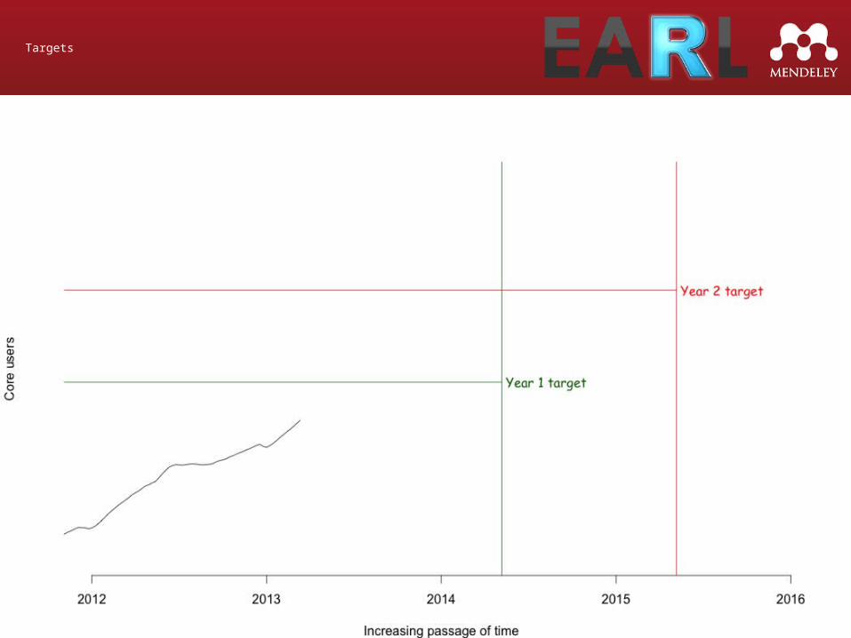
Targets

Graph showing model

Targets

This seems like a reasonable idea

This seems like a reasonable way of measuring it

Ideally we would like to know we are increasing core users when we make software changes

Can we do some analysis?

Properties of Core Users

Long term, hard to see cause and effect

We have an issue with delayed event capture

Estimated Core Users is not a very good estimate

Our usage is very seasonal

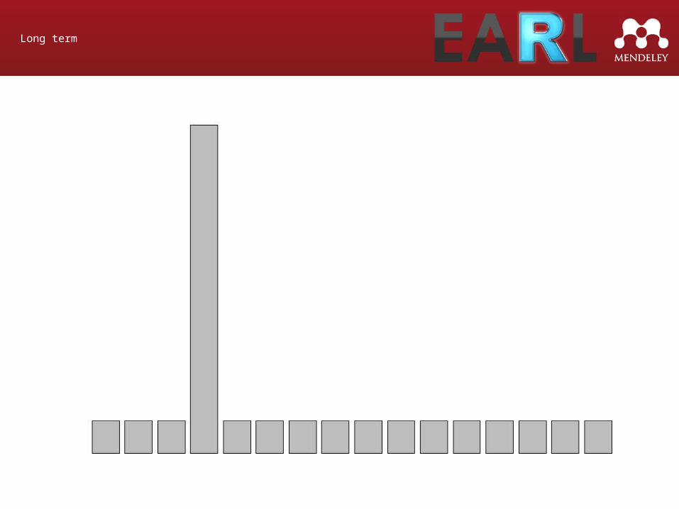
Long term

Messages arriving after the event

Classifiers

Estimated core users is a prediction of becoming a measured core user

How good a prediction is it?

Measuring classifiers

Precision: if we predict someone will be a Measured Core User, how likely is it they will be?

Recall: if someone becomes a measured core user, how likely is it that we predicted this?

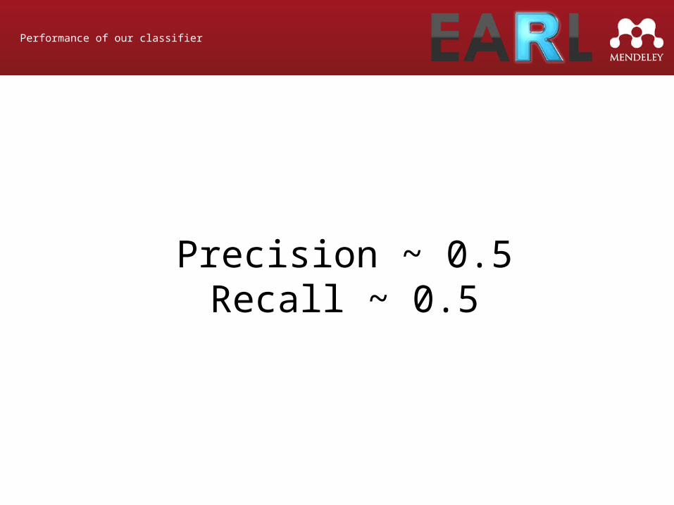
Performance of our classifier

Precision ~ 0.5Recall ~ 0.5

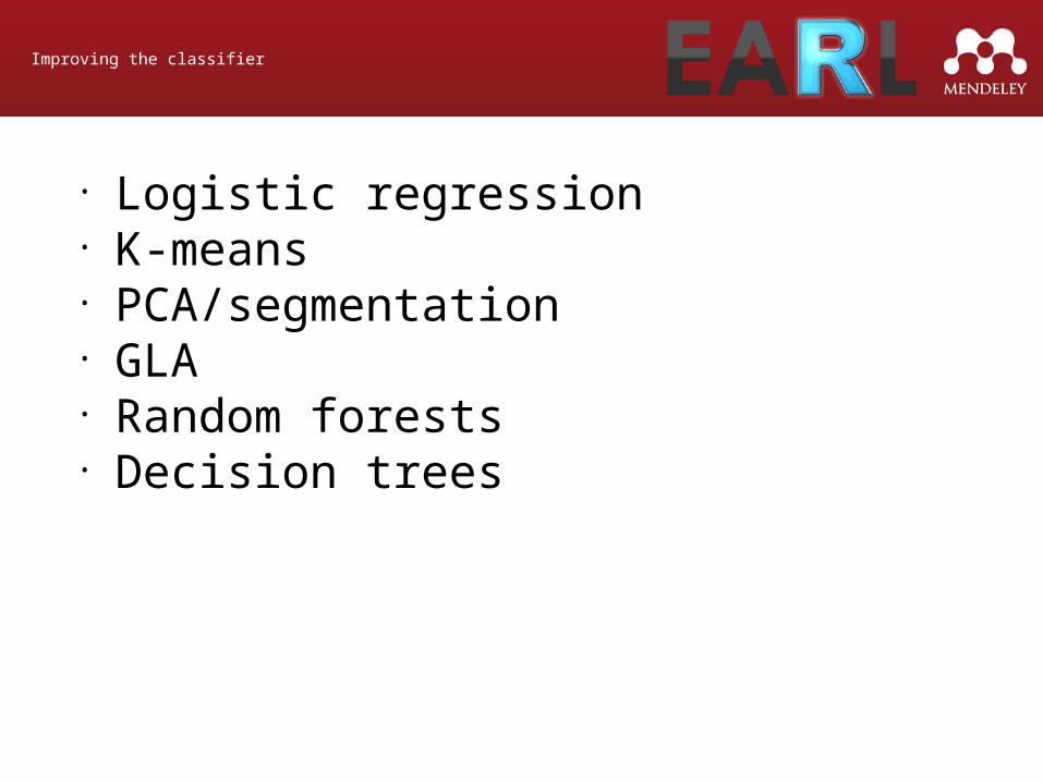
Improving the classifier

• Logistic regression• K-means• PCA/segmentation• GLA• Random forests• Decision trees

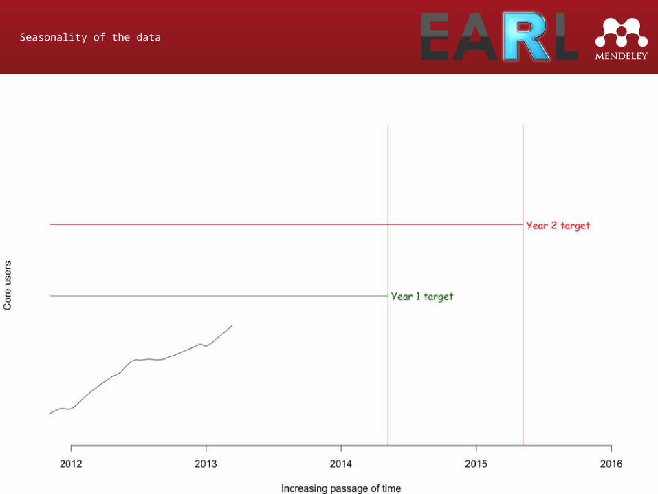
Seasonality of the data

Graph showing model

STL

Seasonal Decomposition of Time Series by Loess (Cleveland et al 1990)

Decomposes into seasonal, trend and remainer

Cleveland shows that it is performant even for long data series

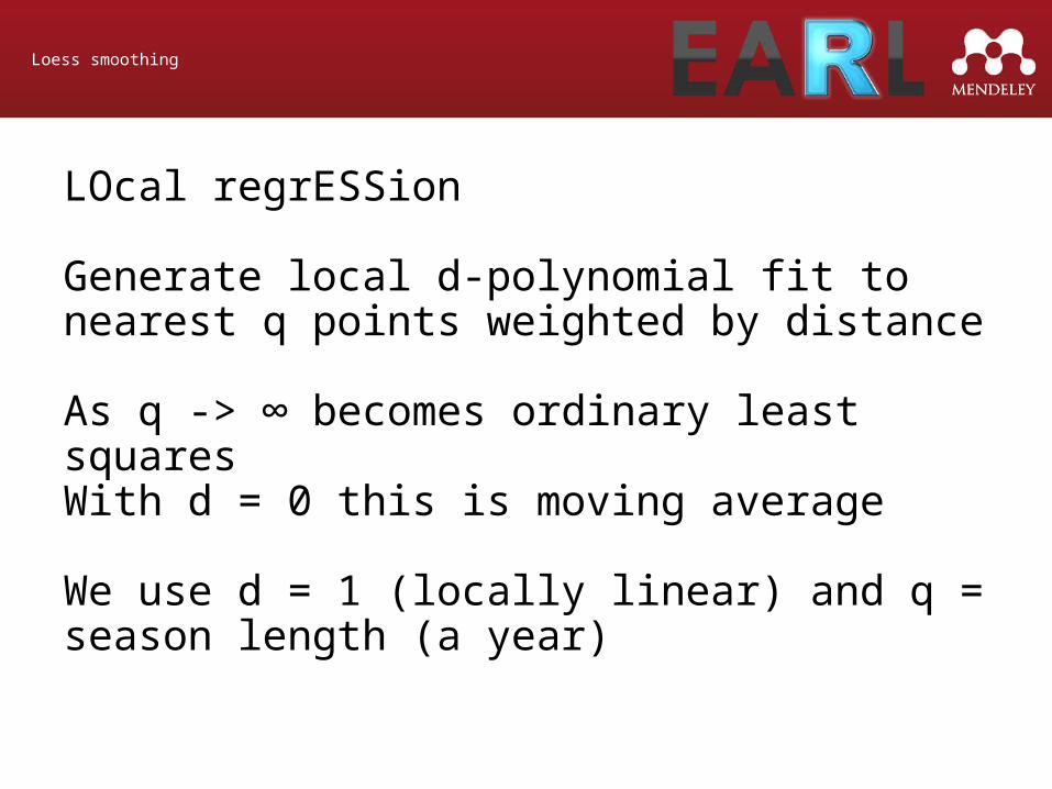
Loess smoothing

LOcal regrESSion

Generate local d-polynomial fit to nearest q points weighted by distance

As q -> ∞ becomes ordinary least squaresWith d = 0 this is moving average

We use d = 1 (locally linear) and q = season length (a year)

STL

• We want to calculate Y=S+T+R• STL works iteratively • We use an initial value for T = 0 • We only use the ‘inner loop’ and only

iterate twice but you can also use an ‘outer loop’

• STL then post smooths the seasonal component

For the parameters we use this is...

• Calculate Y - T• Break into cycle-subseries• Smooth the above with loess to give C• Low pass filter of C to give L • Detrend C by calculating C - L to give new

S• Smooth Y - S to give new T• Repeat• Smooth S and calculate R as Y – S - T

Code

series <- read.table(file="data.csv", header=F, sep=";")$V2

myts <- ts(data=series, start=c(2011, 43), frequency=52)

mystl <- stl(myts, s.window="periodic")

plot(mystl)

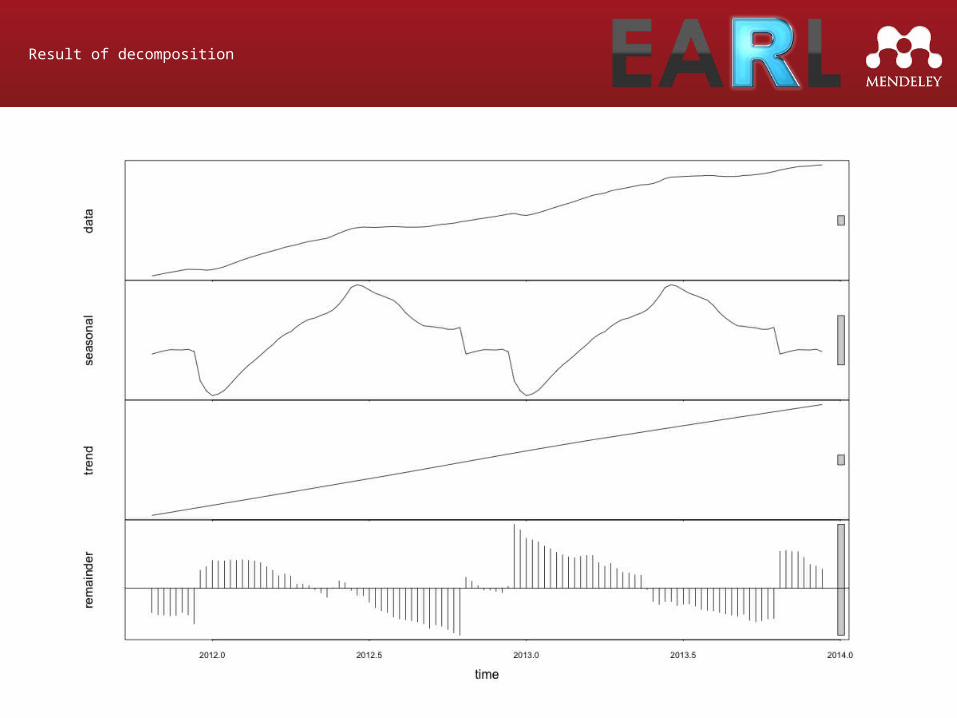
Result of decomposition

[Graph of decomp]

Prediction

Take the trend

Use a linear model to predict future trend

Add back in the seasonal

Add in some error estimates based on fit

There is an R package for this on CRAN

Code

library(forecast)

mystlf <- stlf(ts, s.window="periodic")

plot(mystlf)

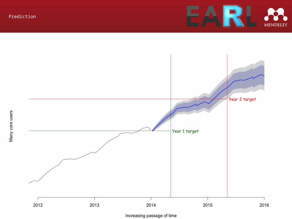
Prediction

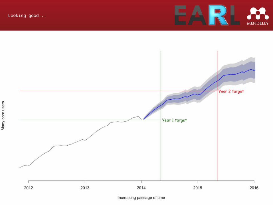
Looking good...

Looking ok...

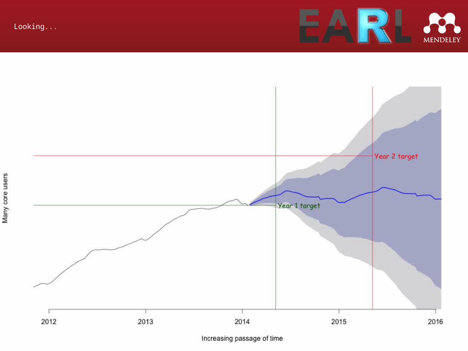
Looking...

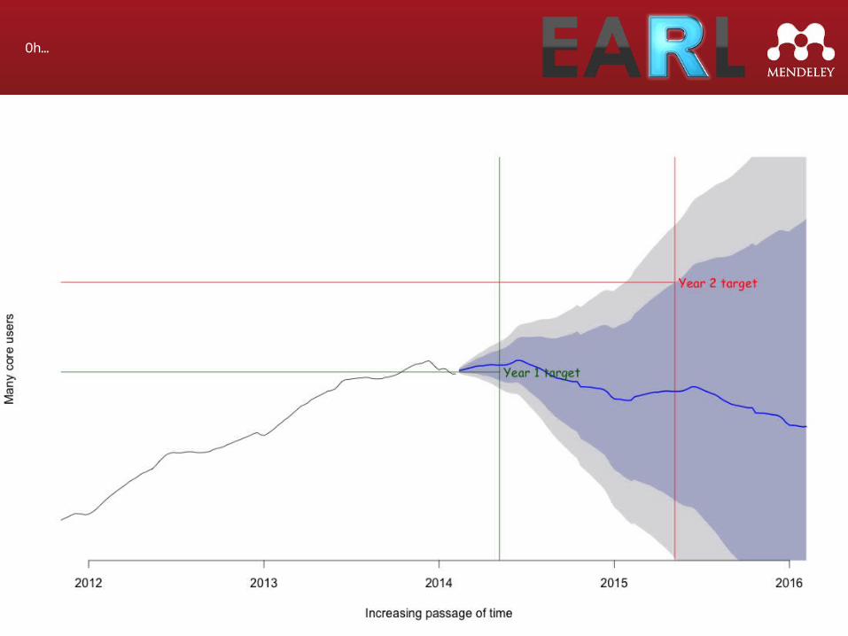
Oh…

What happened?

?

Prediction vs Reality

[Graph of prediction]

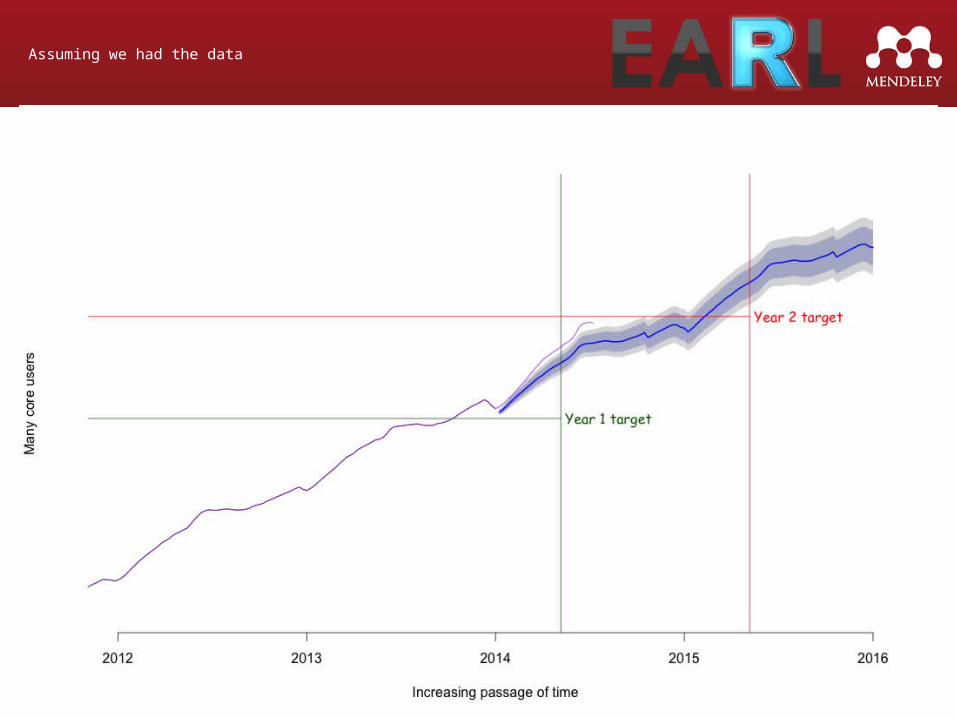
Assuming we had the data

Why are we underestimating?

Possibilities:• The underlying trend is not linear• We’re doing better than expected:

– iOS app– integration with other products– improvements to existing products

Where are we now?

We might already have hit the target

Once new messages come in we should exceed the target

Very high chance of success (according to our model)

It could still go wrong...

Next steps

Can we improve our results by assuming a non linear trend?

Can we use seasonality to make better predictions?

Can we feed core user estimates back into our design process?

Does the metric need changing?

Communication

Toilet stats[picture of toilet]

Questions

?