The Compromise Effect in Post-Purchase Consumption of Complementary Products: A Meta-Analysis of Experimental

Studies

Masters Thesis

Kerstin Beatrice Lehmeier

Spring Term 2018

Chair of Quantitative Marketing and Consumer Analytics L5, 2 - 2. OG 68161 Mannheim www.quantitativemarketing.org

Advisor: Veronica Valli

II

Table of Content

List of Abbreviations ................................................................................................................ IV

List of Figures ........................................................................................................................... V

List of Tables ............................................................................................................................ VI

Abstract ................................................................................................................................... VII

1. Introduction ........................................................................................................................ 1

2. Methodological Foundation of the Meta-Analysis ............................................................. 2

2.1 Introduction to Meta-Analysis ..................................................................................... 2

2.2 Effect Size of Individual Studies ................................................................................. 4

2.2.1 Definition and overview. ........................................................................................ 4

2.2.2 Unstandardized mean difference. ........................................................................... 5

2.2.3 Standardized mean difference ................................................................................ 6

2.3 Fixed-Effect and Random-Effects Model .................................................................... 7

2.4 Measurement and Interpretation of Heterogeneity .................................................... 10

3. Definitions and Research Questions ................................................................................ 13

4. Conceptual Foundation for the Empirical Analysis ......................................................... 15

4.1 Overview and Coding of the Experimental Studies .................................................. 15

4.2 Conceptual Procedure of the Meta-Analyses ............................................................ 17

5. Empirical Analysis and Results........................................................................................ 19

5.1 Meta-Analyses of Aspects of Post-Purchase Consumption ...................................... 19

5.1.1 Sum of complementary products .......................................................................... 19

III

5.1.2 Amount of money spent on complementary products. ........................................ 23

5.1.3 Amount of time spent on choosing complementary products. ............................. 25

5.2 Meta-Analyses of the Evaluation of the Compromise Choice .................................. 28

5.3 Meta-Analyses of the Evaluation of the Choice of Complementary Products .......... 31

6. Discussion ........................................................................................................................ 34

6.1 Summary of the Main Findings ................................................................................. 34

6.2 Managerial Implications ............................................................................................ 35

6.3 Limitations and Future Research ............................................................................... 35

Tables ....................................................................................................................................... 37

Figures ...................................................................................................................................... 40

Appendix .................................................................................................................................. 47

References ................................................................................................................................ 81

Affidavit ................................................................................................................................... 86

IV

List of Abbreviations

C Control group

CI95 95% confidence interval

ES Effect size

FM Fixed-effect model

H0 Null hypothesis

MA Meta-analysis

MAD Mean absolute deviation

mTurk Amazon Mechanical Turk

PI95 95% prediction interval

RM Random-effects model

RQ Research question

S Estimated standard deviation

σ Standard deviation of the population

SE Standard error

SG Subgroup

SMD Standardized mean difference

T Treatment group

T1 Treatment 1 group

T2 Treatment 2 group

θ True effect size

UMD Unstandardized mean difference

Y Observed effect

V

List of Figures

Figure 1: Meta-Analyses 1 and 2 on Sum of Complementary Products .................................. 40

Figure 2: Meta-Analyses 3 and 4 on Amount of Money Spent on Complementary Products . 41

Figure 3: Meta-Analyses 5 and 6 on Amount of Time Spent on Choosing

Complementary Products ......................................................................................... 42

Figure 4: Meta-Analyses 7 and 8 on the Satisfaction with the Compromise Choice ............... 43

Figure 5: Meta-Analyses 9 and 10 on the Confidence in the Compromise Choice ................. 44

Figure 6: Meta-Analyses 11 and 12 on the Difficulty of the Compromise Choice ................. 45

Figure 7: Meta-Analyses 13 to 18 on Evaluation of the Choice of Complementary Products 46

VI

List of Tables

Table 1: Overview of Research Questions, Meta-Analyses and Underlying Studies .............. 37

Table 2: Overview of the Experimental Studies ...................................................................... 38

Table 3: Overview of the Results of All Meta-Analyses ......................................................... 39

VII

Abstract

Marketing research increasingly uses the method meta-analysis to integrate the results of the

growing number of studies. This thesis applies this approach to the field of consumer behavior,

which has most frequently published meta-analyses in marketing. The methodological

foundation regarding the meta-analyses conducted on the compromise effect and post-purchase

consumption are presented. The compromise effect is an important and variously demonstrated

context effect. The thesis investigates how a compromise decision influences the choice of

complementary products and how these two choices made are evaluated. 18 meta-analyses

summarize the results of 15 studies conducted by this chair. They apply distinct effect sizes and

both fixed-effect and random-effects models. Participants, who compromise, tend to select

more complementary products, spend more money and take less time for this decision.

Respondents are less satisfied and confident with their compromise choice and find it more

difficult to make it. Participants, who compromise, are less satisfied and confident with their

decision on additional products and perceive this choice as more difficult in the studies. The

findings indicate implications for practitioners and future research.

Keywords: meta-analysis, fixed-effect and random-effects model, compromise effect,

consumer behavior

1

Introduction

The influence of contextual factors on consumer behavior has been frequently investigated in

marketing literature (Lichters et al. 2016, p. 184). The compromise effect is one of the most

important context effects (Kivetz, Netzer, and Srinivasan 2004, p. 238). It states that the

“market share” (Simonson 1989, p. 159) of an option increases if it is displayed as middle or

compromise option in a set of alternatives. The relevance of this effect is undeniable for

marketing strategies like branding or the positioning of products and its impact on sales

(Neumann, Böckenholt, and Sinha 2016, p. 195). This thesis aims at addressing how a purchase

decision of a product made under a compromise effect further influences the post-purchase

consumption of its complementary products. The research questions include whether people,

who compromise, behave differently in terms of how many additional products they select, how

much money they spend and how much time they need for this decision. Moreover, the thesis

examines how people evaluate the compromise choice and the decision of complementary

products in terms of satisfaction, confidence and difficulty.

To answer these questions, 18 meta-analyses based on up to 15 experimental studies are

conducted. In the marketing field, the method meta-analysis is increasingly applied for

“integrating the findings” (Glass 1976, p. 3) across various individual studies (Grewal,

Puccinelli, and Monroe 2018, p. 9). The methodological foundations required for these meta-

analyses are presented in detail.

Consequently, the thesis starts presenting the method meta-analysis before specifying

the research questions. Furthermore, the underlying experimental studies are described and the

empirical results of the numerous meta-analyses are reported and interpreted. A discussion

finally sums up the key findings, shows managerial implications and identifies limitations and

interesting further research directions.

2

Methodological Foundation of the Meta-Analysis

1.1 Introduction to Meta-Analysis

The method meta-analysis (MA) was introduced by Gene V. Glass in the mid of the seventies

and is a “statistical analysis of a large collection of analysis results from individual studies for

the purpose of integrating the findings” (Glass 1976, p. 3). Its aim is to “accumulate knowledge”

(Grewal, Puccinelli, and Monroe 2018, p. 9) regarding a specific research question or field. It

summarizes the outcome of various studies by computing a “numerical measure” (Eisend 2015,

p. 27) regarding the link of two research variables and presents the magnitude and the

significance of this effect. The MA further examines both consistency and differences across

studies and analyzes potential sources of heterogeneity (Churchill Jr. and Peter 1984, p. 360;

Grewal, Puccinelli, and Monroe 2018, p. 9; McShane and Böckenholt 2017, p. 1048). It helps

to synthesize the outcome of a growing number of publications and summarizes the current

state of research (Grewal, Puccinelli, and Monroe 2018, p. 23; Palmatier, Houston, and Hulland

2017, p. 2). It allows “empirical generalization” (Hanssens 2018, p. 6) based on the amount of

underlying studies and derives further theoretical and practical implications. It has a broad field

of application like medicine, health, social and business sciences (Hartung 2008, p. 2; Johnson,

Mullen, and Salas 1995, p. 94). According to the review paper of Grewal, Puccinelli, and

Monroe (2018) on seventy-four MAs in highly-ranked marketing journals, MAs are constantly

used in marketing since 1985, with an increase in application from 2000 on. The consumer

behavior, product management, communication and sales most frequently use MAs.

The method “vote-counting” marks the beginning of synthesizing studies. A common

effect is derived by comparing the sum of positive and negative significant study results

(Hedges and Olkin 1980, p. 359). Low sample sizes and low underlying effects, however,

reduce power substantially (Hedges and Olkin 1980, p. 359).

3

Based on the work by Glass (1976), Schmidt and Hunter (1977) and Rosenthal (1978),

various MAs approaches have evolved (Grewal, Puccinelli, and Monroe 2018, p. 11; Hall and

Brannick 2002, p. 377). The procedure by Hedges and his colleagues (Hedges 1981, 1982;

Hedges and Olkin 1985; Hedges and Vevea 1998) and the so-called Hunter-Schmidt method

(Schmidt and Hunter 2015) are applied most (Ellis 2010, p. 109; Hall and Brannick 2002, p.

377). Aguinis et al. (2011) show, that the choice of a specific approach does not substantially

impact the magnitude of the effect size. In line with the majority of MAs in marketing, the

thesis uses “standard recommended meta-analytic techniques” (Grewal, Puccinelli, and Monroe

2018, p. 12), which are presented by the book of Borenstein et al. (2010) referring to the

approach by Hedges and his colleagues.

Several steps structure the procedure of a MA. After specifying the research questions

and variables, the appropriate effect size and the model to integrate, i.e. fixed-effect or random-

effects model, are chosen (Grewal, Puccinelli, and Monroe 2018, p. 20). In case of too high

diversity and unavailability of data for the calculation of the effect sizes, p-values of the primary

studies are used (Borenstein et al. 2010, p. 326). Effect sizes are preferred since p-values only

investigate whether “the effect is probably not zero” (Borenstein et al. 2010, p. 325). Next, the

collection of all relevant publications on the research objective, ranging from journal articles to

dissertations and manuscripts, follows (Lipsey and Wilson 2001, p. 25). The coding of the data

based on a coding scheme involves capturing all study characteristics, which may cause

variation between studies like the year, authors and the research design, and summarizing the

necessary data to calculate the effect sizes (Grewal, Puccinelli, and Monroe 2018, p. 15;

Schulze, Holling, and Böhning 2003, p. 12). The quality of the studies are evaluated regarding

how the studies fit the research objective and how adequate the techniques applied are (Cooper

2010, p. 85). Finally, the integration of the studies leads to a common effect (Hartung 2008, p.

8). The heterogeneity of the data is assessed by subgroup analysis or meta-regression. A

4

sensitivity analysis checks the robustness of the findings regarding methodological assumptions

(Cooper 2010, p. 106). Guidelines like the meta-analysis reporting standards (MARS) capture

how to present results in an understandable way (Cooper 2010, p. 219).

In the following, all methodological consideration relevant for this thesis are presented.

Effect Size of Individual Studies

Definition and overview. The effect size (ES) determines “the strength of a relationship

or the magnitude of a difference between variables” (Peterson, Albaum, and Beltramini 1985,

p. 97) or groups in the underlying population (Borenstein et al. 2010, p. 17; Fern and Monroe

1996, p. 90). It measures "the degree to which the null hypothesis is false" (Cohen 1977, pp. 9–

10). ESs are calculated on study level and then integrated across trials (see 2.3) (Fern and

Monroe 1996, p. 90; Grewal, Puccinelli, and Monroe 2018, p. 11). The ES is chosen according

to the research objective, the availability of data, the comparability and interpretability across

all trials (Borenstein et al. 2010, p. 18). Various ESs exist: means, odds or risk ratios in case of

binary data and correlations for correlational data (Borenstein et al. 2010, p. 19; Ellis 2010, p.

13). As this thesis compares the means of a treatment group (T) and a control group (C) based

on separate samples, ESs based on means of independent groups are selected. Various forms,

i.e. the unstandardized mean difference (UMD) and different types of the standardized mean

difference (SMD), are required to account for distinct scale characteristics of the research

variables across studies and to compare results based on different ESs as part of a sensitivity

analysis. The individual ESs are directly computed from primary data. Methods to estimate ESs

from test statistics like t- or F-values are described in Borenstein et al. (2010).

The variances of the ESs are an essential component for the integration of the ESs. Their

calculation depends on whether the standard deviations of the underlying populations (σ) of T

and C are equal, i.e. σT = σC = σ (Grissom and Kim 2005, p. 53). The Levene-test investigates

5

the frequently violated assumption of homogeneity of variance and indicates whether this

equation is met by the data, as equal variances imply same standard deviations of the two

populations (Grissom and Kim 2005, p. 53). If the test is statistically significant, the null

hypothesis (H0) of equal population variances, i.e. σ²T = σ²C = σ², is rejected and the two

populations have unequal variances and so different standard deviations (Bühl 2016, p. 284).

The following sections use the notation and the formulas which are derived from basis

literature, especially Borenstein et al. (2010), Hartung and Knapp (2003) and Schulze (2004).

Unstandardized mean difference. The UMD is used if all studies share the same scale

(Borenstein et al. 2010, p. 21). The population mean difference (Δ) is based on the population

means of T (µT) and C (µC) and is estimated by D, using sample mean T (M̅T) and C (M̅C)

∆ = μT

- μC

D = M̅T - M̅C

(Borenstein et al. 2010, pp. 21–22). As M̅C is subtracted from M̅T, the sign of D indicates

whether the treatment has a positive effect, if M̅T > M̅C, or negative effect, if M̅T < M̅C

(Grissom and Kim 2005, p. 53). The variance of the ES (VD) is calculated based on the Levene-

test result. If H0 of homogenous variances is rejected and thus the standard deviations differ,

VD with the standard deviations of T (ST) and C (SC) and sample size of T (nT) and C (nC) is

VD = ST

2

nT +

SC2

nC

(Borenstein et al. 2010, p. 22). Otherwise, VD uses the pooled standard deviation (Spooled)

(Grissom and Kim 2005, p. 60; Hedges 1981, p. 110). The standard error (SED) equals the

square root of VD (Borenstein et al. 2010, p. 22).

VD = nT + nC

nT nC * Spooled

2 with

Spooled = √(nT - 1) ST

2 + (nC - 1) SC2

nT + nC - 2

6

Standardized mean difference. The SMD is applied if studies contain different scales to

measure a research variable (Grissom and Kim 2005, p. 49). It standardizes the mean difference

of T and C by dividing it by a standard deviation so that the SMD can be compared across trials

(Glass 1977, p. 371). It is a “measure of overlap between distributions” (Borenstein et al. 2010,

p. 26). Depending on variance heterogeneity, either the SMD Glass’ d or Hedges’ g is required.

Glass’ d (ΔGlass), developed by Gene V. Glass, is needed if studies reveal

heteroscedasticity (Glass 1977, p. 370). It only uses the standard deviation of C to standardize

and is estimated by d based on the respective sample values

∆Glass = μT - μC

σC

d = M̅T - M̅C

SC

(Glass 1977, p. 370). The ES Glass’ d indicates the difference between T and C in terms of

standard deviation of C (Glass 1977, p. 371). The variance (Vd) is

Vd = √(nT + nC)

nT nC+

d²

2(nT - 1)

(Hartung 2008, p. 15). If heterogeneity is not the case, the usage of Spooled for standardization is

appropriate. Spooled, presented above, is preferred over Sc in Glass’ d as it considers both samples

(Hedges 1981, p. 109). Spooled is a “less biased and a less variable estimator of σ” (Grissom and

Kim 2005, p. 53). This ES is called Hedges’ g (gpop) and is estimated by g

gpop

= μT - μC

σ

g = M̅T - M̅C

Spooled

(Grissom and Kim 2005, p. 54; Hedges 1981, p. 110). However, the ES tends to be

overestimated – the smaller the sample size and the higher the value of the ES of the population

are (Grissom and Kim 2005, p. 54; Hedges 1981, p. 112). So, g is adjusted (gadj) by multiplying

it with the approximation of a correction term with degrees of freedom (df) of nT + nC - 2

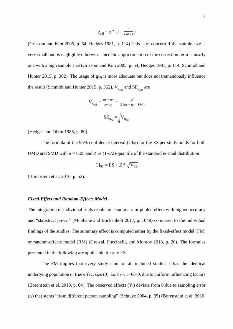
7

gadj

= g * (1 - 3

4 df - 1)

(Grissom and Kim 2005, p. 54; Hedges 1981, p. 114) This is of concern if the sample size is

very small and is negligible otherwise since the approximation of the correction term is nearly

one with a high sample size (Grissom and Kim 2005, p. 54; Hedges 1981, p. 114; Schmidt and

Hunter 2015, p. 362). The usage of gadj is more adequate but does not tremendously influence

the result (Schmidt and Hunter 2015, p. 362). Vgadj and SEgadj

are

Vgadj =

nT + nC

nT nC +

g2

2 (nT + nC - 3.94)

SEgadj=√Vgadj

(Hedges and Olkin 1985, p. 80).

The formula of the 95% confidence interval (CI95) for the ES per study holds for both

UMD and SMD with α = 0.05 and Z as (1-α/2)-quantile of the standard normal distribution

CI95 = ES ± Z * √VES

(Borenstein et al. 2010, p. 52).

Fixed-Effect and Random-Effects Model

The integration of individual trials results in a summary or pooled effect with higher accuracy

and “statistical power” (McShane and Böckenholt 2017, p. 1048) compared to the individual

findings of the studies. The summary effect is computed either by the fixed-effect model (FM)

or random-effects model (RM) (Grewal, Puccinelli, and Monroe 2018, p. 20). The formulas

presented in the following are applicable for any ES.

The FM implies that every study i out of all included studies k has the identical

underlying population or true effect size (θ), i.e. θ1=…=θk=θ, due to uniform influencing factors

(Borenstein et al. 2010, p. 64). The observed effects (Yi) deviate from θ due to sampling error

(εi) that stems “from different person sampling” (Schulze 2004, p. 35) (Borenstein et al. 2010,

8

p. 64). The summary effect (M) is a weighted mean of Yi over all studies and weighting factor

(Wi) per study i is the inverse of its within-study variance (VYi) (Borenstein et al. 2010, p. 65)

M = ∑ Wi Yi

ki=1

∑ Wiki=1

Wi = 1

VYi

.

This “minimize(s) the variance of the pooled estimate” (Schulze 2004, p. 36) by giving more

weight to more accurate Yi as the quotient rises with smaller VYi. The variance of M (VM) is

computed “as the reciprocal of the sum of the weights” (Borenstein et al. 2010, p. 66) and the

standard error (SEM) as the square root of VM

VM = 1

∑ Wiki=1

.

In contrast, the RM assumes that the true effect size per study i (θi) varies across studies

(Hedges 1983, p. 389). The parameter θi result from “a super-population of effects with mean”

(Hartung and Knapp 2003, p. 56) µ and with a between-study variance (τ²) (Hedges 1983, p.

391). The true effect sizes θi of the trials incorporated reflect “a random sample“ (Borenstein et

al. 2010, p. 61) and follow a normal distribution. The variation of Yi is based on εi per study i

and the between-study variance τ² (Borenstein et al. 2010, p. 71). The weighting factor Wi* of

the estimated summary effect (M*) includes the within-study variance VYi per study, like in the

FM, and the estimated between-study variance of τ² (T²)

M* = ∑ Wi

* Yi

ki=1

∑ Wi*k

i=1

Wi* =

1

VYi + T²

(Borenstein et al. 2010, p. 73). The computation of T² is explained in section 2.4 in detail. The

measures of the RM are all marked with *. The weights of the RM are “more balanced”

(Borenstein et al. 2010, p. 85) since the consideration of T² increases the proportional

9

importance of Wi* of small trials and decreases Wi

* for larger studies. VM* , with SEM

* as its square

root, is calculated as

VM* =

1

∑ Wi*k

i=1

.

The 95% prediction interval (PI95) presents the “distribution of true effect sizes” (Borenstein et

al. 2010, p. 133) with α = 0.05, df = k - 2 and value t as

PI95 = M* ± tdfα * √T2 + V

M* .

The formula of the CI95 and of the test of significance of the pooled effect hold for both

FM and RM. The CI95 uses α = 0.05 and Z as the (1-α/2)-quantile of the standard normal

distribution. It reveals how precise M and M* are (Borenstein et al. 2010, p. 5). The CI95 of the

RM is wider as it includes within- and between-study variance (Borenstein et al. 2010, p. 85).

CI95 = M ± Z * √VM or CI95 = M* ± Z * √VM* .

A significance test for the H0 of zero true effect is essential. The FM sets H0: θ = 0 and the test

of the RM considers H0: µ = 0, i.e. that the mean of all true effect sizes θi (µ) is zero (Borenstein

et al. 2010, p. 330; Schulze 2004, p. 40). The test is based on a Z-value, which is checked

against “a crucial value from the standard normal distribution” (Schulze 2004, p. 37). The two-

sided p-value is computed with the cumulative standard normal distribution Ф(Z) (Borenstein

et al. 2010, p. 298)

Z = M

SEM or Z* =

M*

SEM*

p = 2(1 - (Φ(|Z|)) or p* = 2(1 - (Φ(|Z*|)).

FM and RM differ in terms of the conclusions they allow and in their applicability

(Grewal, Puccinelli, and Monroe 2018, p. 20). The findings of a RM can be transferred to the

population, which the included studies form a sample of (Hedges 1983, p. 389). Thus, the results

10

are generalizable while the outcome of the FM is restricted to the studies included in the MA

(Hedges and Vevea 1998, p. 488). A FM is feasible if the included trials are “functionally

identical” (Borenstein et al. 2010, p. 83) and if the same parameters have an impact on the

individual effect sizes. McShane and Böckenholt (2017) suggest, however, that heterogeneity

even plays a role in MAs with very similar studies. Thus, the usability of this model is restricted

due to the specific and rarely fulfilled assumptions (Schulze 2004, p. 35). In contrast, the RM

considers other factors than sampling error alone and assumes that the true effect sizes differ

between studies (Hedges 1983, p. 389; Schmidt and Hunter 2015, p. 366). A test of significance

is useful to examine whether heterogeneity across studies exists (see section 2.4 for details).

The test, however, should not be conducted in advance to indicate a specific model (Hedges

and Vevea 1998, p. 500). Accordingly, the choice should be based on the understanding of the

characteristics of the underlying data and the test result should encourage this decision (Hedges

and Vevea 1998, p. 500). However, in case that the test is significant, i.e. the H0 of equal true

effect sizes across studies is rejected, a FM is inappropriate (Grewal, Puccinelli, and Monroe

2018, p. 20). The choice of a RM is preferred due to the limited applicability of the FM and due

to the fact that the FM is a subtype of the RM as an RM with a between-study variance of zero

mathematically becomes a FM (Schmidt and Hunter 2015, p. 222).

Measurement and Interpretation of Heterogeneity

In line with the RM, numerous influencing factors next to the sampling error exist, which cause

variation of the effects, e.g. “methodological characteristics” (Grewal, Puccinelli, and Monroe

2018, p. 10) like sample source, data collection method or variable measurement.

The test for homogeneity, firstly described by Hedges (1982), examines the presence of

heterogeneity. It addresses the H0 whether the same true effect size underlies all incorporated

trials, i.e. H0: θ1=…=θk=θ, or accordingly the between-study variance (τ²) equals zero (Hedges

11

1982, p. 493; Pigott 2012, p. 56). If Ho holds, the parameter Q closely follows a χ²-distribution

with df=k-1 (Borenstein et al. 2010, p. 112; Cochran 1954, p. 114; Hedges 1982, p. 493)

Q = ∑ Wi(Yi - M)²ki=1 .

Q captures the total variation, which is observed from study to study, and df represents the

anticipated magnitude of Q if the total variation only stems from sampling error (Borenstein et

al. 2010, p. 109). Wi and M are calculated as presented in section 2.3. A significant outcome

results in the rejection of H0 and indicates that distinct true effect sizes underlie the trials

(Hedges 1982, p. 493). An insignificant test does not imply homogeneity since the power of the

test may be decreased due to a low amount of trials and high inaccuracy of the studies included

(Borenstein et al. 2010, p. 113; Hedges 1982, p. 493).

Following measures examine how large heterogeneity is. As important component of

the RM, τ² describes the variance between the individual studies and captures how the true

underlying ES varies across studies. It is measured as T² based on the DerSimonian and Laird

method or “method of moments” with df = k -1 as

T2 = Q - df

C with

C = ∑ Wi ki=1 -

∑ Wi2k

i=1

∑ Wiki=1

(Borenstein et al. 2010, p. 114; DerSimonian and Laird 1986, p. 182). A negative value of T²,

which is possible if Q-df is negative, is changed to zero (Borenstein et al. 2010, p. 114).

The parameter I² based on the work by Higgins and Thompson (2002) and Higgins et

al. (2003) captures the share of the variation which results from heterogeneity and not from

sampling error (Grewal, Puccinelli, and Monroe 2018, p. 21). It is a relative value between 0%

and 100% and is changed to zero if the parameter is negative (Higgins et al. 2003, p. 558). Its

advantage is its independence of the number of studies included (Higgins et al. 2003, p. 557)

I2 = 100% * Q - df

Q .

12

The degree of I² is divided into “low” with 25%, “moderate” with 50% and “high” beginning

with 75% (Higgins et al. 2003, p. 557). I² is an indicator of how consistent the studies are

(Higgins et al. 2003, p. 558). A large value of I² requests a more detailed analysis of the

underlying reasons for the heterogeneity in terms of a subgroup analysis or meta-regression

(Borenstein et al. 2010, p. 122; Higgins et al. 2003, p. 559). In contrast to the subgroup analysis,

the meta-regression analysis accounts for various factors at once (Grewal, Puccinelli, and

Monroe 2018, p. 21). Various subgroup analyses are conducted in the course of this thesis.

Based on a moderator, the studies are assigned to distinct subgroups (SG) and a mean effect

size is computed per individual SG (Borenstein et al. 2010, p. 149). The subgroup analysis

applies the RM as well and uses the same parameters and procedures for M* and Wi* per SG

like previously for all studies together. As according to Borenstein et al. (2010) a number of

less than five studies per SG can decrease the precision of T², a pooled parameter (Twithin²) is

calculated based on the sum of the individual measures Q, df and C per SG j with m as the total

number of SGs

Twithin2 =

∑ Qj - ∑ dfjmj=1

mj=1

∑ Cjmj=1

.

Otherwise, T² is computed individually per SG j (Borenstein et al. 2010, p. 164). If the

moderator has an influence, the distinct SGs reveal smaller heterogeneity, i.e. a lower value of

I² compared to the overall heterogeneity, and the differences between the mean effect sizes of

the SGs are statistically significant (Borenstein et al. 2010, p. 119; Grewal, Puccinelli, and

Monroe 2018, p. 22). The “Q-test for heterogeneity” (Borenstein et al. 2010, p. 178) already

presented above examines whether the estimated mean effect size per SGs are statistically

significant. The SGs are treated as if they were individual studies and – instead of the individual

ES and its variance – the mean effect size and the according variance per SG are used as input

(Borenstein et al. 2010, p. 170).

13

Finally, a sensitivity analysis examines the robustness of the findings regarding

underlying methodological assumptions and investigates whether the results are consistent

(Cooper 2010, p. 106). The analysis contrasts the results based on distinct ES measures. It

further investigates the influence of single studies on the overall effect by excluding every study

and recalculating the summary effect.

Definitions and Research Questions

The compromise effect was firstly shown by Simonson (1989) and describes that the choice of

an alternative is more likely when it becomes the middle or compromise option “with

intermediate attribute values relative to the choice set” (Dhar and Simonson 2003, p. 147)

(Simonson 1989, p. 161). Extremeness aversion of the customers induces this behavior – in

case a customer is uncertain regarding the preferences of “different combinations of attribute

values” (Simonson 1989, p. 158) (Simonson and Tversky 1992, p. 282; Tversky and Simonson

1993, p. 1183). The choice of the middle option is “easier to justify and less likely to be

criticized” (Simonson 1989, p. 168). Neumann, Böckenholt, and Sinha (2016) show the

robustness of this consumer behavior in their meta-analysis based on 72 distinct studies. Many

more publications demonstrate this effect in various contexts and conditions (Kivetz, Netzer,

and Srinivasan 2004, p. 238; Lichters et al. 2016, p. 184).

The focus of this thesis goes beyond the objective of the studies on the compromise

effect as it especially investigates the influence of a product choice made under the compromise

effect on the post-purchase consumption of complementary products. The thesis covers various

research questions (RQ) and aims at gaining a first insight regarding these effects. In terms of

the choice of complementary products, the sum of items chosen, the amount of money and the

14

time spent on selecting additional products are examined. The complementarity of a product

includes that the decrease of the price of one product results in the sales growth of a second

product (Shocker, Bayus, and Kim 2004, p. 28). This implies that the products are utilized

together in order to fulfill a certain customer’s need (Walters 1991, p. 18).

Further RQs refer to the evaluation of the product decisions: choice satisfaction,

confidence and difficulty are examined for both the compromise decision and the choice of

complementary products.

The specific RQs of this thesis are presented in Table 1 (insert Table 1 about here). For

each research variable, the RQs distinguish between two options, A and B, which are presented

as compromise option in the treatment conditions in the primary studies. The experimental

design of the primary studies is presented in more detail in section 4.1. The RQs are:

Does a product choice made under the compromise effect influence

(1) the sum of complementary products in case of option B (RQ1.1) and option A (RQ1.2)

as compromise option?

(2) the amount of money spent on choosing complementary products in case of option B

(RQ2.1) and option A (RQ2.2) as compromise option?

(3) the amount of time spent on choosing complementary products in case of option B

(RQ3.1) and option A (RQ3.2) as compromise option?

Does a product choice made under the compromise effect influence

(4) the satisfaction with this choice in case of option B (RQ4.1) and option A (RQ4.2) as

compromise option?

(5) the confidence in this choice in case of option B (RQ5.1) and option A (RQ5.2) as

compromise option?

(6) the difficulty to make this decision in case of option B (RQ6.1) and option A (RQ6.2)

as compromise option?

15

Does a product choice made under the compromise effect influence

(7) the satisfaction with the choice of complementary products in case of option B (RQ7.1)

and option A (RQ7.2) as compromise option?

(8) the confidence in the choice of complementary products in case of option B (RQ8.1)

and option A (RQ8.2) as compromise option?

(9) the difficulty to make the decision on complementary products in case of option B

(RQ9.1) and option A (RQ9.2) as compromise option?

Conceptual Foundation for the Empirical Analysis

Overview and Coding of the Experimental Studies

The bases for the MAs form 15 studies conducted by this chair. The studies involve a between-

study design with participants, who are randomly assigned to either a control condition or to

one of the two treatment groups. They form independent groups (Koschate 2008, p. 116).

In these studies, participants are firstly asked to make a purchase decision on a specific

product, named choice 1. Respondents can select from different alternatives of a product. These

options differ on two attributes, which involve a trade-off. For example, distinct camera types

ranging from a cheap and low-quality to an expensive, top-quality camera are presented. The

two treatment conditions show three distinct alternatives to choose from and thus create a

situation in which the participant might compromise, i.e. select the middle option. Treatment 1

group (T1) sees options A, B and C with B as middle option and Treatment 2 group (T2) is

exposed to alternatives A’, A and B with A as compromise. The control group (C) only includes

A and B. The respondents, who select the compromise option B in T1 or alternative A in T2

are compared to the respective participants selecting A and B in C. The difference between T1

16

and T2 is that alternative A is compromise option in T2 and the lower extreme in T1, while

option B is the middle option in T2 and the upper extreme in T1.

Secondly, participants make a choice on complementary products, called choice 2. In

anticipation of a prospective situation, in which they would utilize the product of choice 1, they

are asked whether they would consider buying one or more of 10 additional products.

Accordingly, 10 distinct complementary items are displayed, which are derived from the

recommendations on Amazon for the product in choice 1.

Thirdly, respondents are asked to evaluate both choice 1 and 2 regarding satisfaction,

confidence and difficulty.

The chair conducted a total of ten study runs. In each run, respondents see two or three

different products and thus make two or three choices 1 and 2, i.e. they make choice 1 and 2

regarding a first product like a laptop with additional items and a second product like a camera

with complementary camera products. As an unrelated filler task separates these different

products in the study, the answers are considered to be independent. After excluding the

preliminary study runs 1.a and 2.a and test run 7 on a differing research focus, a sum of 15

different trials are used for the MA.

To use the studies in a MA, the coding of all studies regarding their characteristics and

the relevant data is necessary (Lipsey and Wilson 2001, p. 85). Every test gets a unique study

ID. The trials share almost the same survey and procedure but differ in terms of the type of

products displayed and the sample source as presented in Table 2 (insert Table 2 about here).

Studies involve choices on durables like a camera, consumables like a toothbrush and services

as a gym membership. Test 1 to 7 use students of the University of Mannheim and study 8 to

15 apply the qualified workforce called Amazon Mechanical Turk (US only) (mTurk).

Furthermore, the basic data, from which all MA parameters are derived, is calculated.

This includes the mean, the standard deviation and the sample size per each research variable,

17

group and study. Pivot tables in Excel compute the data for MA1 to MA6 and STATA computes

the remaining values. In MA5 and MA6 on the time spent on choice 2, the primary data requires

an adjustment. The group means of a few tests stand out with very high values ranging from

25.062 in test 2 to 40.445 seconds in test 9 in MA6. These figures result from only a few

participants with values ranging from 142.217 seconds to about 11 minutes. As the time

tracking finally ends with the submission of the page of the survey, a participant might report

these long durations in case of distraction or interruption. Four high values are identified in

study 7 in MA5 and test 2, 8 and 9 in MA6 and are excluded. These so called “outliers” also

comply with the criteria of the detection method described by Wilcox (2010, p. 33), which uses

the median absolute deviation (MAD). It indicates an observation X as outlier if following

equation holds, with X̅ as mean

|X - X̅| > 2 * MAD

0.6745.

Conceptual Procedure of the Meta-Analyses

The objective of this thesis is to combine the findings of the 15 experimental studies outlined

above and address the RQs by 18 MAs. Table 1 also gives an overview of all MAs regarding

the specific RQs. The number of incorporated studies varies since not all variables are covered

by every test. This section outlines the general procedure and assumptions underlying the MAs.

It is based on the methodological foundation of MAs presented above. All MAs are programed

in Excel. The Excel Add-in “MetaXL” is used to compute key measures and figures (Barendregt

and Doi n.d., p. 10). MetaXL, however, only considers the formula of the variance of the UMD

according to variance heterogeneity. The Excel file further includes the output of the Levene-

tests from STATA.

For every MA, a forest plot and a table condense the findings. A forest plot is a graph

that displays the individual ESs per study, the CIs and the summary effect (Borenstein et al.

18

2010, p. 366). To enable a general overview per research variable, the figures contain the MAs

for both options of comparison A and B.

Every MA starts with the choice of a suitable ES and its calculation depending on two

criteria. Firstly, either a UMD or SMD depending on whether the scale of the research variable

is identical across trials is selected. Secondly, the presence of heteroscedasticity influences the

choice of the formula for the variance of UMD and the type of SMD. The values of the Levene-

tests are based on the sample means (Bühl 2016, p. 284). If the Levene-tests report

heteroscedasticity, the variance of the UMD requires the formula based on variance

heterogeneity (see 2.2.2) and the SMD Glass’ d is appropriate. Otherwise, the other variance

formula and the adjusted Hedges’ g are applied. When one test out of the MAs on the same

research variable shows heteroscedasticity, both MAs align their ES choice. A RM is generally

assumed since it is the preferred model as discussed in section 2.3. Alpha is 0.05 for all MAs.

Afterwards, the MAs compute and interpret heterogeneity measures. In case of high

heterogeneity, which is reflected by a high I², a subgroup analysis evaluates both content-related

and methodological influencing factors on the ESs. So, the impact of the type of product and

the sample source is assessed. According to the product displayed in the study, tests 1, 3 and 6

form the subgroup “consumable”, studies 2, 4, 8 to 16 the group “durable” and finally tests 5

and 7 “service” (see Table 2). Consumables are products that are consumed during usage

whereas durables are products which are used over a longer period of time (Sander 2011, p.

364). Services are immaterial goods, which cannot be stored and which are provided in close

contact between provider and receiver (Sander 2011, p. 364). Due to the few studies per group,

the measure T²within is applied; otherwise T² is calculated per group separately (see 2.4). Despite

the low number of trials per subgroup, the analysis gives a first insight into the effects.

In the end, the sensitivity of the results is investigated regarding following issues, if

required. Firstly, MetaXL is used to compute how the outcome changes if every individual

19

study is excluded from the calculation of the summary effect. For MA13 to 16 the values are

calculated in Excel as MetaXL does not support the required formula as described above.

Secondly, different ES measures are applied. If a UMD is appropriate, its result is contrasted

with the finding based on either Glass’ d or Hedges’ g depending on the occurrence of

heteroscedasticity. If a MA initially applies Glass’ d, the MA is also performed with Hedges’ g

to compare both results as the results might deviate since the standard deviations used for

standardization in the denominator might vary (Fern and Monroe 1996, p. 90). Thirdly, the

results based on both sample sources, i.e. students and mTurk, are contrasted.

Empirical Analysis and Results

Meta-Analyses of Aspects of Post-Purchase Consumption

Sum of complementary products. MA1 and MA2 address how a compromise choice

affects the number of complementary products chosen. MA1 targets RQ1.1 with option B as

compromise comparing T1 and C and MA2 focuses on RQ 1.2 with T2 and C regarding middle

option A. The “sum of complementary products” reflects the total amount of chosen items. The

research variable sums up diverse complementary products, e.g. camera items or laptop items

depending on the product in choice 1, across studies. Thus, a SMD is needed. Glass’ d is used

since the Levene-tests detect heteroscedasticity in following studies: tests 3 (F = 9.313,

p < 0.01), 5 (F = 17.003, p < 0.001) and 11 (F = 4.838, p < 0.05) in MA1 and trials 3 (F = 8.052,

p < 0.01), 4 (F = 6.805, p < 0.05), 5 (F = 4.460, p < 0.05), 6 (F = 9.980, p < 0.01) and in MA2

test15 (F = 8.419, p < 0.01). Glass’ d is measured in standard deviation of C since the difference

between the means of T and C are divided by the standard deviation of C. Figure 1 concludes

the results of MA1 and MA2, which are presented in the following (insert Figure 1 about here).

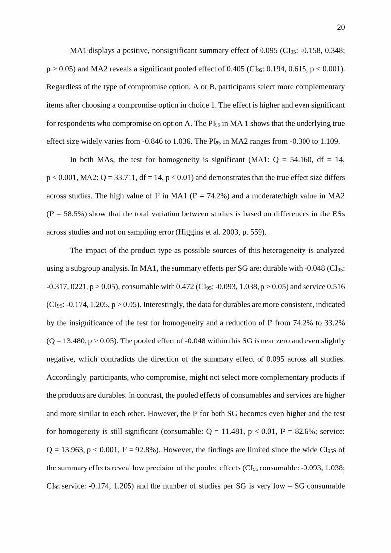
20

MA1 displays a positive, nonsignificant summary effect of 0.095 (CI95: -0.158, 0.348;

p > 0.05) and MA2 reveals a significant pooled effect of 0.405 (CI95: 0.194, 0.615, p < 0.001).

Regardless of the type of compromise option, A or B, participants select more complementary

items after choosing a compromise option in choice 1. The effect is higher and even significant

for respondents who compromise on option A. The PI95 in MA 1 shows that the underlying true

effect size widely varies from -0.846 to 1.036. The PI95 in MA2 ranges from -0.300 to 1.109.

In both MAs, the test for homogeneity is significant (MA1: Q = 54.160, df = 14,

p < 0.001, MA2: Q = 33.711, df = 14, p < 0.01) and demonstrates that the true effect size differs

across studies. The high value of I² in MA1 (I² = 74.2%) and a moderate/high value in MA2

(I² = 58.5%) show that the total variation between studies is based on differences in the ESs

across studies and not on sampling error (Higgins et al. 2003, p. 559).

The impact of the product type as possible sources of this heterogeneity is analyzed

using a subgroup analysis. In MA1, the summary effects per SG are: durable with -0.048 (CI95:

-0.317, 0221, p > 0.05), consumable with 0.472 (CI95: -0.093, 1.038, p > 0.05) and service 0.516

(CI95: -0.174, 1.205, p > 0.05). Interestingly, the data for durables are more consistent, indicated

by the insignificance of the test for homogeneity and a reduction of I² from 74.2% to 33.2%

(Q = 13.480, p > 0.05). The pooled effect of -0.048 within this SG is near zero and even slightly

negative, which contradicts the direction of the summary effect of 0.095 across all studies.

Accordingly, participants, who compromise, might not select more complementary products if

the products are durables. In contrast, the pooled effects of consumables and services are higher

and more similar to each other. However, the I² for both SG becomes even higher and the test

for homogeneity is still significant (consumable: Q = 11.481, p < 0.01, I² = 82.6%; service:

Q = 13.963, p < 0.001, I² = 92.8%). However, the findings are limited since the wide CI95s of

the summary effects reveal low precision of the pooled effects (CI95 consumable: -0.093, 1.038;

CI95 service: -0.174, 1.205) and the number of studies per SG is very low – SG consumable

21

including 3 studies and SG service with 2 trials. The comparison of the pooled effects across

all SGs further reveals that the dispersion of the outcomes does not result from differences in

the SG across the distinct product types but from sampling error. This finding is based on the

insignificant test for homogeneity across SGs (Q = 4.232, df = 2, p > 0.05). Consequently, the

product type does not explain the heterogeneity and does not lead to distinct effects across SGs.

However, this finding is to be considered with caution as the test might erroneously be

insignificant due to low power as described above (see section 2.4).

In contrast to MA1, the subgrouping by product type in MA2 leads to very similar

summary effects across SGs including durable with 0.402 (CI95: 0.135, 0.668, p < 0.01),

consumable with 0.443 (CI95: -0.147, 1.034, p > 0.05) and service with 0.370 (CI95: -0.228,

0.967, p > 0.05). The pooled effect is significant for durables (p < 0.01). I² is reduced to 49.9%

but the test for homogeneity is still significant (p < 0.05), which indicates that other factors

explain heterogeneity across studies and the ESs are not consistent as reported by MA1.

Accordingly, heterogeneity is not explained for the consumables: I² even increases to 85.3%

with a significant test for homogeneity (p < 0.01). Contrary to the MA1, the ESs within SG

service are more homogenous as the test for homogeneity is insignificant (p > 0.05) and an I²

of 0.0% shows that any variance results from sampling error. The test for heterogeneity to

compare the mean effects across all SGs is insignificant (Q = 0.030, df = 2, p > 0.05). It implies

that the product type equally influences the SGs so that the underlying true ESs do not vary.

However, the possibly low power of the test is to be considered. In conclusion, both subgroup

analyses report contradictory findings regarding the SGs. They further indicate that the product

type does not seem to influence the sum of complementary products.

Both sensitivity analyses show the robustness of the findings of the MAs. The sensitivity

analysis of MA1 with a pooled effect of 0.095 reveals that the exclusion of any of the tests

results in changes in the summary effect between 0.020 (CI95: -0.200, 0.240) and 0.132 (CI95:

22

-0.127, 0.391). The findings based on Glass’ d are compatible with Hedges’ g pooled effect of

0.061 (CI95: -0.160, 0.281, p > 0.05). The summary effect based on mTurk with -0.043 (CI95:

-0.232, 0.146, p > 0.05) is almost zero in comparison to the studies based on students with a

pooled effect of 0.302 (CI95: -0.222, 0.826, p. > 0.05). Interestingly, the studies based on

students are significantly heterogeneous (Q = 32,946, df = 6, p < 0.001) while the trials based

on mTurk are more consistent (Q = 10.318, df = 7, p > 0.05). However, the effects do not

significantly differ between the two groups (Q = 1.475, df = 1, p > 0.05). In MA2 with a

summary effect of 0.405, the single exclusion of any of the tests leads to changes in the pooled

effect between 0.347 (CI95: 0.156, 0.537) and 0.450 (CI95: 0.247, 0.653). The implications of

the effect based on Hedges’ g does not deviate from Glass’ d with 0.343 (CI95: 0.183, 0.503, p

< 0.001). Referring to sample source students, the summary effect is 0.524 (CI95: 0.092, 0.956,

p < 0.05) and regarding mTurk this value is 0.300 (CI95: 0.122, 0.479, p < 0.01). As indicated

by the insignificant test for heterogeneity, the findings might not differ (Q = 0.880, df = 1,

p > 0.05). However, the trials using students are significantly heterogeneous

(Q = 20.723, df = 6, p < 0.01), while mTurk-based studies are not (Q = 8.237, df = 7, p > 0.05).

In conclusion, regarding RQ1.1 and RQ1.2, participants, who compromise, select more

additional products. This effect is lower for respondents compromising with option B and even

significant for option A. The product type does not seem to account for differences in the effect.

However, all results need be considered with caution due to the limited number of studies. Other

sources of heterogeneity need to be considered in further analyses. All computed effects are

robust regarding methodological assumptions. The usage of the RM allows the generalizability

of the results to the study population, which the included trials form a sample of.

23

Amount of money spent on complementary products. MA3 and MA4 examine RQ2.1

and RQ2.2 on whether customers who compromise in choice 1 spend more or less money on

complementary products. MA3 focuses on option B as compromise option and MA4 analyzes

option A. The research variable sums up the prices of all items chosen per participant. Again,

the prices are linked to the respective products, i.e. expensive camera items vs. cheaper

toothbrush products. To make them comparable, a SMD is used. Glass’ d is applied as the

Levene-tests report heteroscedasticity for tests 3 (F = 8.642, p < 0.01), 5 (F = 9.831, p < 0.01)

and 7 (F = 6.737, p < 0.05) in MA3 and studies 3 (F = 7.061, p < 0.01), 6 (F = 7.520, p < 0.05)

and 9 (F = 8.534, p < 0.01) in MA4. Figure 2 presents the results (insert Figure 2 about here).

Both MAs reveal a positive effect of the compromise situation on the amount of money

spent on complementary items. The effect of MA3 with option B as compromise option shows

an insignificant summary effect of 0.081 (CI95: -0.154, 0.316, p > 0.05). The PI95 of the true

effect size ranges from -0.318 to 1.002. In contrast, MA4 shows that the participants

compromising on option A spend significantly more money with a pooled effect of 0.342 (CI95:

0.139, 0.544, p < 0.01). The PI95 of the true effect size is -0.300 to 0.975.

The test for homogeneity is significant in both MAs (MA3: Q = 46.893, df = 14,

p < 0.001; MA4: Q = 31.461, df = 14, p < 0.01). The high value of I² in MA3 (I² = 70.1 %) and

a high/moderate value in MA4 (I² = 55.5%) show that the total variation between studies is

based on differences in the ESs across studies. The impact of the product type as potential

reason for this heterogeneity is investigated by a subgroup analysis (Higgins et al. 2003, p. 559).

In MA3, the slightly negative pooled effect of -0.049 (CI95: -0.302, 0.203, p > 0.05) for

durables differs from the other two SGs including consumables with a pooled effect of 0.499

(CI95: -0.039, 1.037) and services with 0.378 (CI95: -0.264, 1.020). The ESs for durables are

more consistent since the test for homogeneity is insignificant (Q = 15.646, df = 9, p > 0.05)

and I² is reduces to 42.5%. It becomes obvious that the studies in the other two SGs are very

24

heterogenous. Both SGs show very wide CI95s of their summary effect, I² even increases

(SG consumable: I² = 79.5%, SG service: I² = 88.9%) and the test for homogeneity remains

significant for both SGs (p < 0.01). Thus, the product type does not source heterogeneity, which

is also supported by the insignificant test of heterogeneity to compare the SGs

(Q = 4.159, df = 2, p > 0.05).

In contrast, to MA3, MA4 reveals more similar pooled effects per SG: durables with a

pooled effect of 0.352 (CI95: 0.101, .604, p < 0.01), consumables with a summary effect of

0.466 (CI95 -0.103, 1.035, p > 0.05) and services with 0.167 (CI95: -0.395, 0.729, p > 0.05). The

effect is, however, only significant for durables. Heterogeneity is an issue as well. An I² of

55.5% shows that only half of the variance is based on real differences between the studies.

Subgrouping by product type does not lead to a decrease of heterogeneity for durables with an

I² of 54.8% and a significant test for homogeneity (Q = 19.891 df = 9, p < 0.05). The same holds

for consumables with an I² of 77.9% and a significant test for homogeneity (Q = 9.069, df = 2,

p < 0.05). Both SGs are highly inconsistent and other influencing factors, which are not

considered yet, play a role. In contrast, an I² of 0.0% and an insignificant test for homogeneity

(Q = 0.563, df = 2, p > 0.05) in SG service indicate that only sampling error causes variation.

The test on whether the underlying true effect sizes of the individual SGs are equal is

insignificant (Q = 0.563, df = 2, p > 0.05). In line with MA3, the findings show that the product

type probably does not lead to differences in the true effect sizes between SGs.

The sensitivity analysis for both MAs show that the methodological assumptions only

lead to slight differences in the computed effects. In MA3 with a pooled effect of 0.081, the

omission of single studies leads to a variation in the summary effect from 0.016 (CI95: -0.191,

0.224) to 0.115 (CI95: -0.125, 0.355). The result of Hedges’ g is very similar with a pooled

effect of 0.045 (CI95: -0.161, 0.252, p > 0.05). The comparison of the mean effect sizes of

25

students and mTurk is insignificant (Q = 1.893, df = 1, p > 0.05). In contrast to the mTurk trials,

the studies with students are significantly heterogeneous (Q = 24.607, df = 6, p < 0.001).

In MA4, the results are robust as well with a significant summary effect of 0.342. The

exclusion of any single study shows a pooled effect ranging from 0.288 (CI95: 0.105, 0.471) to

0.385 (CI95: 0.185, 0.585). Hedges’ g reveals very similar results with a summary effect of

0.305 (CI95: 0.125, 0.485, p < 0.01). A comparison of the estimated mean effect sizes between

studies using students and mTurk as sample source is not significant (Q = 0.544 df = 1,

p > 0.05). The pooled effect in both SGs are significant and vary only slightly: the estimated

mean effect size using students is 0.441 (CI95: 0.035, 0.846, p < 0.05) and the result based on

mTurk is 0.269 (CI95: 0.061, 0.477, p < 0.05). In line with previous findings, the studies using

students are significantly heterogeneous (Q = 18.536, df = 6, p < 0.01).

With regard to RQ2.1 and 2.2, both MAs show that participants who compromise tend

to spend more money on complementary products. This effect is only significant for MA4 with

option A as middle option. The results on the role of the product type indicate that the

underlying true effect sizes are not influenced by it. However, these findings are limited to the

low number of studies included and need to be considered with caution. The findings are not

sensitive to methodological assumptions. As the RM is applied, the results are generalizable to

the large population from which the studies incorporated here form a sample of.

Amount of time spent on choosing complementary products. MA5 and MA6 focus on

whether participants who compromise spend more or less time on the decision of the

complementary items. MA5 addresses participants compromising on option B in T1 (RQ3.1)

and MA6 examines respondents selecting option A as middle option in T2 (RQ3.2). The time

is measured in seconds and covers the period of time that participants need for their decision

on complementary products. The time tracking ends with the submission of the page. In total,

26

4 extreme values are excluded from primary data as described in section 4.1. The UMD is

applied, since the variable is comparable across studies. The Levene-tests of trial 2 (F = 4.091,

p < 0.05) and test 9 (F = 5.627, p < 0.05) in MA6 report heteroscedasticity and thus the variance

of UMD is calculated accordingly (see 2.2.2). Tests 3 to 5 do not track time and are excluded.

Although the RM is preferred, the analysis of heterogeneity parameter reveals that it is

not the suitable approach. In line with Borenstein et al. (2010), the choice between FM and RM

should not be based on heterogeneity but rather on theoretical considerations. However, a misfit

between the assumption and the results should lead to a reconsideration of the initial choice

(Hedges and Vevea 1998, p. 500). In this case, a RM is expected as the studies are not identical

and various influencing factors might have an impact. However, the heterogeneity parameters

do not support this choice. Figure 3 concludes all results (insert Figure 3 about here).

Firstly, the MAs report an insignificant test for homogeneity (MA5: Q = 3.999, df = 11,

p > 0.05; MA6: Q = 9.045, df = 11, p > 0.05). The insignificance does not mean that the ESs

are homogeneous and thus the RM is inappropriate. The test can be low in power due to a small

number of trials and a high variation of the individual ESs based on sampling error. However,

further heterogeneity measures should be considered (Borenstein et al. 2010, p. 113).

Secondly, I² and T² are analyzed, which are independent of the number of trials included.

They are equal to zero in both MAs. An I² of zero shows that all variation is based on sampling

error and a search for the reasons for heterogeneity by a subgroup analysis becomes

unnecessary. A between-study variance T² of zero mathematically reduces the RM to a FM.

Thirdly, the forest plots show that the variation of the ESs per study are in the range of

the CI95s. This means that the sampling error within the studies is the reason for the variation

and not between-study variance. This further indicates that the FM is the appropriate model.

Finally, it is examined whether SMDs report the same results. The outcome based on

Glass’ d and Hedges’ g are in line with the UMD. Regarding Glass’ d, the test for homogeneity

27

is also insignificant for both MAs (MA5: Q = 4.446, df = 11, p > 0.05, MA6: Q = 11.083,

df = 11, p > 0.05). T² and I² are zero in MA5 and near zero in MA6 with T² of 0.001 and I² of

0.7%. Hedges’ g also leads to an insignificant test for homogeneity (MA5: Q = 4.317, df = 11,

p > 0.05; MA6: Q = 7.815, df = 11, p > 0.05) and reports a zero value for T² and I².

In conclusion, the assumption of the RM is rejected as the heterogeneity measures do

not support this model. Consequently, a FM is applied to integrate the findings of the trials.

Based on the FM, both MAs present an insignificant and slightly negative summary

effect. Participants, who compromise in choice 1, need minimally less time to decide on

complementary products than participants in the control condition. The insignificant negative

summary effect of -0.156 (CI95: -1.756, 1.444, p > 0.05) in MA5 shows that participants

compromising on option B need 0.156 seconds less. This effect is higher for MA6 with an

insignificant pooled effect of -0.853 (CI95: -2.409, 0.704, p > 0.05). However, the wide CIs

imply low precision of the summary effect. According to the FM, these effects only hold for

the studies of the MAs and cannot be generalized to other studies (Cooper 2010, p. 191). The

FM also indicates that the studies are identical regarding the research variable time and share

equal parameters that influence the trials (Borenstein et al. 2010, p. 63).

The sensitivity analysis shows the robustness of the findings in case of the exclusion of

every single study. MA5 with a pooled effect of -0.156 shows a range of -0.018 (CI95: -1.638,

1.675) to 0.137 (CI95: -1.697, 1.953). The summary effects in MA6 with a pooled effect of

-0.853 vary between -1.383 (CI95: -3.025, 0.260) to -0.546 CI95: -2.154, 1.063). The comparison

of these results with findings based on SMDs shows that the SMDs lead to a smaller pooled

effect of almost zero. Using Glass’ d leads to a pooled effect of -0.002 (CI95: -0.139, 0.136,

p > 0.05) in MA5 and to a pooled effect of -0.011 (CI95: -0.159, 0.137, p > 0.05) in MA6. It

indicates that there is almost no difference regarding the time required to make a decision

between participants, who compromise, and respondents, who make a choice without a

28

compromise situation. These results are in line with Hedges’ g with a pooled effect of -0.008

(CI95: -0.145, 0.129, p > 0.05) in MA5 and a summary effect of -0.046 (CI95: -0.192, 0.100, p

> 0.05) in MA6.

To sum it up, the calculated effects are limited to the included trials due to the

application of a FM and RQ3.1 and RQ3.2 are only answered for these studies. Regardless of

the type of compromise option, participants who compromise require insignificantly and

slightly less time on choosing complementary products.

Meta-Analyses of the Evaluation of the Compromise Choice

MA7 to 12 investigate whether participants evaluate a compromise choice differently than

respondents who select this alternative without a compromise situation. RQs 4.1, 4.2, 5.1, 5.2,

6.1 and 6.2 include the satisfaction, the confidence and the difficulty regarding this decision for

either compromise option B or A. In total, 12 trials form the bases for the MAs. Before each

aspect is analyzed in detail, general considerations holding for all MAs are presented.

As the scales of the research variables are identical in all tests, an UMD is applied as

ES. Research variables are measured on a five-point Likert scale with 1 = “not satisfied at all”

and 5 = “completely satisfied” as well as 1 = “not confident at all” and 5 = “completely

confident”. Difficulty of the decision is captured by 1 = “not difficult at all” and 5 = “extremely

difficult”. Due to the heteroscedasticity contained in various tests, the according formula for

the variance of UMD is used for all MAs (see 2.2.2) and Glass’ d as SMD is applied as part of

the sensitivity analysis. A RM is assumed for all MAs. Apart from MA11, all tests for

homogeneity are insignificant, which means that the null hypothesis of homogeneous effects

across studies cannot be rejected. This insignificance should not be taken, however, as an

indicator for homogeneity as the test has limited power, if the variance within the studies is

high and the amount of trials is low (Borenstein et al. 2010, p. 113). A subgroup analysis is not

29

necessary, since all T² values are near zero and the I² figures are very small, which indicate low

heterogeneity across studies. The studies based on mTurk are weighted more due to a lower

within-study variance than the trials using students.

RQ4.1 and 4.2 aim at investigating the choice satisfaction and are targeted by MA7 and

MA8, which are presented in Figure 4 (insert Figure 4 about here). The Levene-tests report

heteroscedasticity in MA7 in test 2 (F = 6.300, p < 0.05) and in study 5 (F = 4.492, p < 0.05)

and in test 9 of MA8 (F = 4.978, p < 0.05). Both MAs report a significant negative pooled

effect. Consequently, participants, who make a compromise choice, are significantly less

satisfied with their decision than respondent who chose this option in a set of two alternatives.

The summary effect with compromise option B in MA7 is -0.250 (CI95: -0.356, -0.144,

p < 0.001) and the pooled effect in MA8 with middle option A -0.141 (CI95: -0.267, -0.015,

p < 0.05). In contrast to the initial considerations, the heterogeneity measures of MA7 reveal

equal results for both FM and RM as T² is zero. The forest plot also implies that all studies

share the exact same underlying true effect size as the individual ESs lie within the CI95s. Thus,

the FM is applied which means that the result of MA7 only holds for the studies investigated.

The sensitivity analysis shows the robustness of the results. In MA7 with a pooled effect

of -0.250, the pooled effect varies between -0.288 (CI95: -0.405, -0.172) and -0.215 (CI95:

-0.333, -0.098) if single studies are excluded. Glass’ d also infers the same with a summary

effect of -0.339 (CI95: -0.478, -0.199, p < 0.001). The omission of single trials in MA8 with a

pooled effect of -0.141 results in a range of pooled effects from -0.168 (CI95: -0.290, -0.046) to

-0.110 (CI95: -0.232, 0.013). The ES Glass’ d also leads to a significant negative summary effect

of -0.190 (CI95: -0.352, -0.029, p < 0.05).

MA9 and MA10 answer RQ5.1 and RQ5.2 on choice confidence, presented in Figure 5

(insert Figure 5 about here). The Levene-tests identify variance heterogeneity in test 9

(F = 9.196, p < 0.05), test 11 (F = 7.550, p < 0.01), test 13 (F = 3.999, p < 0.05) in MA10.

30

Irrespective of the compromise option A or B, respondents are significantly less satisfied with

their decision if they compromise. Both MAs report significant negative pooled effects. The

summary effect of MA9 is -0.366 (CI95: -0.513, -0.219, p < 0.001) and of MA10 -0.339 (CI95:

-0.481, -0.197, p < 0.001). These results are not sensitive regarding single studies and the choice

of the ES. In MA9, the exclusion of single studies leads to a range of the pooled effect from

-0.399 (CI95: -0.564, -0.235) to -0.319 (CI95: -0.443, -0.194) and an effect of -0.435 (CI95:

-0.610, -0.260), p < 0.001) based on Glass’ d. MA10 shows a range of -0.378 (CI95: -0.517,

-0.240) to -0.301 (CI95: -0.446, -0.157) in case of omission of single studies and a pooled effect

of -0.372 (CI95: -0.569, -0.174, p < 0.001) based on Glass’ d.

RQ6.1 and RQ6.2 are about the difficulty of making the compromise choice, which are

addressed by MA11 and MA12, and summarized in Figure 6 (insert Figure 6 about here).

Regardless of the option, participants, who select the alternative as compromise option, evaluate

the level of difficulty of this decision higher than people in the control condition. This effect is

significant for MA12 showing alternative A as compromise option with a pooled effect of 0.355

(CI95: 0.163, 0.546, p < 0.001). This inference does not change if single studies are excluded as

the summary effect changes from 0.304 (CI95: 0.144, 0.464) to 0.397 (CI95: 0.213, 0.580). The

result based on ES Glass’ d, with a pooled effect of 0.275 (CI95: 0.127 0.424, p < 0.001), is also

in line with the outcome of UMD. In contrast, MA11 with compromise option B reports an

insignificant pooled effect of 0.214 (CI95: -0.014, 0.442, p > 0.05). Test 7 on “gym membership”

stands out with a very negative ES of -1.243 as opposed to the remaining studies. A sensitivity

analysis reveals that due to this study the test for homogeneity is significant (Q = 22.281,

df = 11, p < 0.05). Moreover, the exclusion of this test would result in a higher pooled effect of

0.310 and also lead to a significant result (CI95: 0.160, 0.461, p < 0.001). This result is in line

with the summary effect based on Glass’ d of 0.229 (CI95: 0.034, 0.425, p < 0.05). Further

31

research regarding services is required to either exclude this test as outlier or to further

emphasize that influencing factors exist that cause this heterogeneity.

In conclusion, participants, who compromise, are significantly less satisfied with their

decision. This finding is generalizable based on MA8 on option A as compromise. The FM

used in MA7 restricts the outcome to the studies under investigation. Regardless of the type of

compromise option A and B, respondents are further significantly less confident with their

choice, if they select it as a compromise, in comparison to participants who choose these options

in the control condition. Finally, participants who compromise find the decision more difficult

than respondents in the dual option set. The outcome is only significant for option A. The

findings are very consistent as indicated by heterogeneity measures.

Meta-Analyses of the Evaluation of the Choice of Complementary Products

The MAs 13 to 18 examine how participants evaluate their decisions of complementary

products. RQ 7.1, 7.2, 8.1, 8.2, 9.1 and 9.2 address whether participants, who make a

compromise decision in choice 1, evaluate choice 2 on complementary products differently

regarding decision satisfaction, confidence and difficulty than respondents, who do not

compromise in choice 1. Only 6 studies include these research variables. Due to the exclusion

of various studies, the similarity among the tests is relatively high. Their product choices only

cover the durables BBQ grill, camera and laptop and are completely based on mTurk data. A

further issue is the small number of studies. The calculations of a RM based on a small number

of studies result in an imprecise estimate of T² which leads to an inaccurate standard error of

the summary effect and finally affects the CI of the pooled effect (Borenstein et al. 2010, p.

163). Borenstein et al. (2010) suggest the usage of the FM in this case as the FM is already

applicable for two studies and reflects uncertainty of the summary effect by the CI95. Therefore,

all MAs apply an FM and the results are not generalizable and only hold for the included studies.

32

A UMD is required, as the research variables are measured by a 5-point Likert scale like

in the previous MAs on the evaluation of choice 1. The heterogeneity measures do not

contradict the assumption of a FM. All tests for homogeneity report an insignificant result and

both T² and I² are equal or near zero which emphasizes the lack of between-study variance and

the inappropriateness of a subgroup analysis. The forest plots clarify that the variation of the

observed ESs depends on sampling error alone as the individual ES are within the range of the

CI95s, which further supports the usage of the FM. All findings are summarized in Figure 7

(insert Figure 7 about here).

MA13 and MA14 on RQ 7.1 and 7.2 on satisfaction with choice 2 show that participants,

who compromise in choice 1, are significantly less satisfied with their decision on

complementary products. MA13 reports a summary effect of -0.131 (CI95: -0.247, 0.016,

p < 0.05) and MA14 an effect of -0.150 (CI95: -0.285, -0.015, p < 0.05). The variance of UMD

is calculated according to the formula based on variance homogeneity as heterogeneity is not

concluded in the Levene-tests. The findings of both MAs are very robust. The pooled effect of

MA13 varies from -0.172 (CI95: -0.305, -0.039) to -0.114 (CI95: -0.249, 0.021) in case of the

exclusion of every singly trial from the calculation of the results. The pooled effect of -0.179

(CI95: -0.340, -0.019, p < 0.05) based on the standardized measure Hedges’ g is in line with the

findings. Regarding MA 14, the omission of individual studies results in a range of the summary

effect from -0.184 (CI95: -0.335, -0.033) to -0.089 (CI95: -0.241, 0.063). Results with Hedges’

g indicate the same outcome with a pooled effect of -0.184 (CI95: -0.360, -0.008, p < 0.05).

The confidence of choice 2 included in RQ 8.1 and RQ8.2 is examined by MA15 and

MA16. Participants, who make a compromise choice, are significantly less confident regarding

their choice of complementary products. This inference is reflected by the negative summary

effect of -0.157 (CI95: -0.273, -0.040, p < 0.01) in MA15 and a pooled effect of -0.265 (CI95:

-0.406, -0.123, p < 0.001) in MA16. As the Levene-tests do not conclude variance heterogeneity

33

among the studies, the variance of UMD is based on the formula, which does not account for

variance heterogeneity. The sensitivity analyses show the consistency of the results. In MA15,

the exclusion of single trials leads to a range of the pooled effect from -0.191 (CI95: -0.324,

-0.059) to -0.137 (CI95: -0.277, 0.003). Hedges’ g also leads to a significant negative summary

effect of -0.209 (CI95: -0.370, -0.048, p < 0.05). MA16 shows a range from -0.299 (CI95: -0.463,

-0.136) to -0.196 (CI95: -0.356, -0.037) based on the omission of single studies. A pooled effect

based on Hedges’ g of -0.318 (CI95: -0.495, -0.142, p < 0.001) supports the findings.

MA17 and MA18 regarding RQ9.1 and RQ9.2 conclude that participants, who

compromise in choice 1, find it more difficult to make the decision on complementary products.

While MA17 with compromise option B computes a nonsignificant summary effect of 0.093

(CI95: -0.081, 0.267, p > 0.05), MA18 with option A as middle option shows a significant result

with 0.321 (CI95: 0.138, 0.504, p < 0.01). As the Levene-tests report variance heterogeneity in

test 11 (F = 7.689, p < 0.01) and test 12 (F = 6.921, p < 0.05) in MA18, both MAs apply the

variance UMD formula which considers this heterogeneity (see 2.2.2). The findings are not

sensitive to methodological assumptions. The findings of MA17 vary from 0.057 (CI95: -0.143,

0.258) to 0.139 (CI95: -0.046, 0.324) if single studies are excluded. The application of Glass’ d

leads to a similar result of 0.088 (CI95: -0.073, 0.249, p > 0.05). MA18 reports results varying

from 0.281 (CI95: 0.070, 0.492) to 0.371 (CI95: 0.163, 0.579). A summary effect of 0.307 (CI95:

0.128, 0.487, p < 0.01) based on Glass’ d permits the same conclusion like the UMD.

In conclusion, participants, who make a compromise choice first, are significantly less

satisfied and confident regarding their choice of related complementary products and find this

decision more difficult than respondents in the control condition, who make the choices without

compromising. All findings are significant apart from the choice difficulty in case of option B

as compromise alternative. These findings only hold for the studies under investigation as the

FM is applied, which does not allow their generalization.

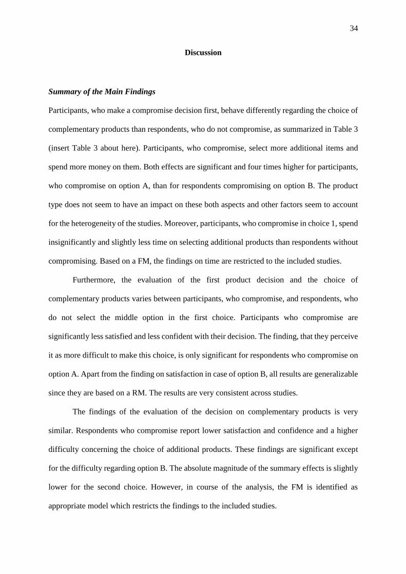
34

Discussion

Summary of the Main Findings

Participants, who make a compromise decision first, behave differently regarding the choice of

complementary products than respondents, who do not compromise, as summarized in Table 3

(insert Table 3 about here). Participants, who compromise, select more additional items and

spend more money on them. Both effects are significant and four times higher for participants,

who compromise on option A, than for respondents compromising on option B. The product

type does not seem to have an impact on these both aspects and other factors seem to account

for the heterogeneity of the studies. Moreover, participants, who compromise in choice 1, spend

insignificantly and slightly less time on selecting additional products than respondents without

compromising. Based on a FM, the findings on time are restricted to the included studies.

Furthermore, the evaluation of the first product decision and the choice of

complementary products varies between participants, who compromise, and respondents, who

do not select the middle option in the first choice. Participants who compromise are

significantly less satisfied and less confident with their decision. The finding, that they perceive

it as more difficult to make this choice, is only significant for respondents who compromise on

option A. Apart from the finding on satisfaction in case of option B, all results are generalizable

since they are based on a RM. The results are very consistent across studies.

The findings of the evaluation of the decision on complementary products is very

similar. Respondents who compromise report lower satisfaction and confidence and a higher

difficulty concerning the choice of additional products. These findings are significant except

for the difficulty regarding option B. The absolute magnitude of the summary effects is slightly

lower for the second choice. However, in course of the analysis, the FM is identified as

appropriate model which restricts the findings to the included studies.

35

Managerial Implications

The various meta-analyses in this thesis enable a first insight into the link between a

compromise choice and the consumption of complementary products. An increase in the

number of complementary items chosen and a higher spending is observed after a compromise

choice on the initial product. The findings provide directions for practitioners in various ways.

Firstly, marketers need to consider that a compromise choice is not only related to the initial

product but also to the choice of complementary items. Consequently, pursuing a product

positioning strategy, which encourages a compromise choice of a product, is also linked to the

sales of its complementary items. Secondly, under the consideration of the compromise effect,

a specific extension of the product range regarding complementary items might be beneficial.

Thirdly, marketing measures like advertising, communication, product placement and pricing

of the products might beneficially influence this effect. Especially in the online context, the

specific presentation of a set of alternatives and complementary products in the form of

recommendations might support this effect. However, the findings of this thesis can only give

a first insight as they are limited in terms of methodological issues and investigated variables.

Limitations and Future Research

A critical evaluation of the conducted meta-analyses reveals that the inferences made are

limited to the characteristics, the variables and the representativeness of the underlying studies

(Rust, Lehmann, and Farley 1990, p. 220). A key issue is the low number of studies, which

imposes challenges on the calculation of measures. Unprecise heterogeneity estimates leading

to inaccurate confidence intervals of the summary effect imply that the findings need to be

considered with caution (Borenstein et al. 2010, p. 363). A subgroup analysis with just two or

three studies per group can only provide a first insight into the underlying effects. Especially,

the required usage of the fixed-effect model in some analyses does not allow the generalization

36

of these findings. The fact that the heterogeneity among studies cannot be fully explained in the

course of the analyses reveals that further methods like a meta-regression analysis and other

variables need to be considered. In contrast to the conducted subgroup analysis, a meta-

regression analysis could consider various moderators in one analysis and thus could give

deeper understanding of the variation across studies (Grewal, Puccinelli, and Monroe 2018, p.

22). Other variables like the composition of the choice set or the type of attributes presented

might further lead to differences in the effects and explain heterogeneity (Neumann,

Böckenholt, and Sinha 2016, p. 193). A meta-analytical structural-equation model could

examine multiple relationships simultaneously (Grewal, Puccinelli, and Monroe 2018, p. 23).

The replication of the studies by further research is very important to increase the

accuracy of the results and to create a wider base for empirical generalizations (Grewal,

Puccinelli, and Monroe 2018, p. 19). Especially, additional studies including services and

consumables are required to examine the effect of the product type in more detail. Furthermore,

the MAs are limited to studies, which ask participants to anticipate a purchase decision. Further

studies should investigate the research questions in real-life purchase situations and thus enable

the comparison of the magnitude and significance of the effects with the current studies. Field

experiments in stores or in an online context could indicate whether the effect differs across

these settings. Other factors might also play a role in the investigated relationship, which are

not addressed by the studies so far, like the influence of the degree of complementarity, which

describes how customers perceive and evaluate “the necessity of one product for the

performance or use of the second product“ (Samu, Krishnan, and Smith 1999, p. 59).

Characteristics of the participants may also have an impact. Customers, named maximizers,

who tend to maximize their value regarding the attributes on alternative, and thus are more

likely to select the middle option in a three-choice, might behave differently in the choice of

complementary products than satisfiers, who focus on only one attribute (Mao 2016, p. 66).

37

Tables

Table 1: Overview of Research Questions, Meta-Analyses and Underlying Studies

Option B Option A

Research variable RQ (T1 vs. C) (T2 vs. C) MA 1 2 3 4 5 6 7 8 9 10 11 12 13 14 15

Aspects of post-purchase consumption

1.1 x MA1

1.2 x MA2

2.1 x MA3

2.2 x MA4

3.1 x MA5

3.2 x MA6

Evaluation of the compromise choice

4.1 x MA7

4.2 x MA8

5.1 x MA9

5.2 x MA10

6.1 x MA11

6.2 x MA12

Evaluation of the choice of complementary products

7.1 x MA13

7.2 x MA14

8.1 x MA15

8.2 x MA16

9.1 x MA17

9.2 x MA18

Note: C = Control group, ID = study identification number, MA = meta-analysis, No. = number, RQ = research question,

T1 = treatment 1 group, T2 = treatment 2 group

Experimental studies: X = research variable included in study

No. of

research

variable

9 X X

1

2

3

4

5

6

7

8

X X

X X X X X X

X X X X

X X X X

X X

X X

X X X X X

X X X X X X

XX X X X

X X X

X X X

X X X X X XX X X

X X X

XX X X X X X X X X

X X X

Difficulty of choice

Option of comparison

Experimental studies included per MA (ID)

X X X X X X

Amount of time spent on

choosing complementary

Satisfaction with choice

Confidence in choice

Difficulty of choice

Satisfaction with choice

Confidence in choice

Sum of complementary

products

X X X X XAmount of money spent

on complementary

X X X X X X

X X X X

X X X X X X

38

Table 2: Overview of the Experimental Studies

ID

Study

run Study name Product Product type

Sample

size Sample source

1 1b 1_Toothbrush Toothbrush Consumable 146 Students of University of Mannheim

2 1b 2_Camera Camera Durable 146 Students of University of Mannheim

3 2b 3_Shampoo Shampoo Consumable 268 Students of University of Mannheim

4 2b 4_Printer Printer Durable 268 Students of University of Mannheim

5 2b 5_Gym membership Gym membership Service 268 Students of University of Mannheim

6 3 6_Laundry detergent Laundry detergent Consumable 152 Students of University of Mannheim

7 3 7_Gym membership Gym membership Service 152 Students of University of Mannheim

8 4 8_BBQ grill BBG grill Durable 152 mTurk participants (US only)

9 4 9_Camera Camera Durable 152 mTurk participants (US only)

10 5a 10_BBQ grill BBG grill Durable 150 mTurk participants (US only)

11 5a 11_Camera Camera Durable 150 mTurk participants (US only)

12 5b 12_BBQ grill BBG grill Durable 363 mTurk participants (US only)

13 5b 13_Camera Camera Durable 363 mTurk participants (US only)

14 6 14_Laptop Laptop Durable 360 mTurk participants (US only)

15 6 15_Camera Camera Durable 360 mTurk participants (US only)

Note: ID = study identification number, mTurk = Amazon Mechanical Turk

Product information Sample

39

Table 3: Overview of the Results of All Meta-Analyses

Option B Option A

Research variable RQ (T1 vs. C) (T2 vs. C) MA Model Effect size Summary effect CI95

Aspects of post-purchase consumption

1.1 x MA1 RM Glass' d 0.095 (-0.158, 0.348)

1.2 x MA2 RM Glass' d 0.405*** (0.194, 0.615)

2.1 x MA3 RM Glass' d 0.081 (-0.154, 0.316)

2.2 x MA4 RM Glass' d 0.342** (0.139, 0.544)

3.1 x MA5 FM UMD -0.156 (-1.756, 1.444)

3.2 x MA6 FM UMD -0.853 (-2.409, 0.704)

Evaluation of the compromise choice

4.1 x MA7 FM UMD -0.250*** (-0.356, -0.144)

4.2 x MA8 RM UMD -0.141* (-0.267, -0.015)

5.1 x MA9 RM UMD -0.366*** (-0.513, -0.219)

5.2 x MA10 RM UMD -0.339*** (-0.481, -0.197)

6.1 x MA11 RM UMD 0.214 (-0.014, 0.442)

6.2 x MA12 RM UMD 0.355*** (0.163, 0.546)

Evaluation of the choice of complementary products

7.1 x MA13 FM UMD -0.131* (-0.247, -0.016)

7.2 x MA14 FM UMD -0.150* (-0.285, -0.015)

8.1 x MA15 FM UMD -0.157** (-0.273, -0.040)

8.2 x MA16 FM UMD -0.265*** (-0.406, -0.123)

9.1 x MA17 FM UMD 0.093 (-0.081, 0.267)

9.2 x MA18 FM UMD 0.321** (0.138, 0.504)

*** p < 0.001, ** p < 0.01, * p < 0.05; alpha = 0.05

Note: C = Control group, CI95 = 95% confidence interval, FM = fixed-effect model, MA = meta-analysis, No. = number,

RM = random-effects model, RQ = research question, T1 = treatment 1 group, T2 = treatment 2 group, UMD = unstandardized mean difference

Option of comparison

1Sum of complementary

products

3Amount of time spent on

choosing complementary

2Amount of money spent

on complementary

No. of

research

variable

6 Difficulty of choice

4 Satisfaction with choice

5 Confidence in choice

9 Difficulty of choice

8 Confidence in choice

7 Satisfaction with choice

40

Figures

Figure 1: Meta-Analyses 1 and 2 on Sum of Complementary Products

RM - Glass' d

Study ID Study name Forest plot Glass' d CI95 Weight Forest plot Glass' d CI95 Weight

1 1_Toothbrush -0.259 (-1.116, 0.598) 4.6% 0.101 (-1.477, 1.679) 1.6%

2 2_Camera -0.231 (-0.833, 0.371) 6.2% 0.439 (-0.174, 1.051) 6.0%

3 3_Shampoo 1.259 (-0.548, 0.769) 6.6% 1.150 (-1.134, 0.274) 7.5%

4 4_Printer 0.311 (-1.534, 0.192) 7.9% 1.269 (-0.476, 0.829) 6.2%

5 5_Gym membership 1.248 (-0.606, 0.433) 6.8% 0.502 (-0.205, 0.959) 8.6%

6 6_Laundry detergent 0.110 (-0.548, 0.769) 5.8% -0.430 (-1.134, 0.274) 5.2%

7 7_Gym membership -0.671 (-1.534, 0.192) 4.5% 0.177 (-0.476, 0.829) 5.6%

8 8_BBQ grill -0.086 (-0.606, 0.433) 6.8% 0.377 (-0.205, 0.959) 6.3%

9 9_Camera -0.031 (-0.643, 0.580) 6.2% 0.173 (-0.330, 0.677) 7.2%

10 10_BBQ grill -0.454 (-1.045, 0.136) 6.3% 0.397 (-0.296, 1.090) 5.3%

11 11_Camera -0.197 (-0.811, 0.417) 6.1% -0.009 (-0.565, 0.547) 6.6%

12 12_BBQ grill -0.149 (-0.491, 0.194) 8.2% 0.274 (-0.124, 0.672) 8.5%

13 13_Camera -0.351 (-0.828, 0.126) 7.2% 0.088 (-0.249, 0.426) 9.3%

14 14_Laptop 0.324 (0.014, 0.634) 8.4% 0.352 (-0.091, 0.796) 7.9%

15 15_Camera 0.123 (-0.201, 0.447) 8.3% 0.785 (0.363, 1.206) 8.2%

Summary effect 0.095 (-0.158, 0.348) 100% 0.405*** (0.194, 0.615) 100%

Heterogeneity and sensitivity analysis

Summary Summary

Model - ES effect CI95 Q df T² I² effect CI95 Q df T² I²

RM - Glass' d 0.095 (-0.158, 0.348) 54.160*** 14 0.173 74.2% 0.405*** (0.194, 0.615) 33.711** 14 0.095 58.5%

Subgroup analysis by product type

Durable -0.048 (-0.317, 0.221) 13.480 9 0.130 33.2% 0.402** (0.135, 0.668) 17.978* 9 0.117 49.9%

Consumable 0.472 (-0.093, 1.038) 11.481** 2 0.130 82.6% 0.443 (-0.147, 1.034) 13.651** 2 0.117 85.3%

Service 0.516 (-0.174, 1.205) 13.963*** 1 0.130 92.8% 0.370 (-0.228, 0.967) 0.704 1 0.117 0.0%

Test for heterogeneity 4.232 2 0.030 2

Sample source

Students 0.302 (-0.222, 0.826) 32.946*** 6 0.395 81.8% 0.524* (0.092, 0.956) 20.723** 6 0.224 71.0%

mTurk -0.043 (-0.232, 0.146) 10.318 7 0.023 32.2% 0.300** (0.122, 0.479) 8.237 7 0.010 15.0%

Test for heterogeneity 1.475 1 0.880 1

RM - Hedges' g 0.061 (-0.160, 0.281) 42.570*** 14 0.119 67.1% 0.343*** (0.183, 0.503) 20.948 14 0.031 33.2%

*** p < 0.001, ** p < 0.01, * p < 0.05; alpha = 0.05

Note: CI95 = 95% confidence interval, ES = effect size, mTurk = Amazon mechancal Turk, RM = random-effects model,

Forest plot (based on MetaXL): square = ES per study (size of square is proportional to weight of study), diamond = summary effect across all studies, horizontal lines = CI 95 per study

Meta-analysis 1: Option B Meta-analysis 2: Option A

Heterogeneity measures Heterogeneity measures

MA2 Glass' d RM

delta1,20-1,2

Study

6_Laundry detergent

11_Camera

13_Camera

1_Toothbrush

9_Camera

7_Gym membership

12_BBQ-Grill

14_Laptop

8_BBQ-Grill

10_BBQ-Grill

Overall

Q=33,71, p=0,00, I2=58%

2_Camera

5_Gym membership

15_Camera

3_Shampoo

4_Printer

delta (95% CI) % Weight

-0,43 ( -1,13, 0,27) 5,2

-0,01 ( -0,57, 0,55) 6,6

0,09 ( -0,25, 0,43) 9,3

0,10 ( -1,48, 1,68) 1,6

0,17 ( -0,33, 0,68) 7,2

0,18 ( -0,48, 0,83) 5,6

0,27 ( -0,12, 0,67) 8,5

0,35 ( -0,09, 0,80) 7,9

0,38 ( -0,21, 0,96) 6,3

0,40 ( -0,30, 1,09) 5,3

0,40 ( 0,19, 0,62) 100,0

0,44 ( -0,17, 1,05) 6,0

0,50 ( 0,11, 0,89) 8,6

0,78 ( 0,36, 1,21) 8,2

1,15 ( 0,67, 1,63) 7,5

1,27 ( 0,68, 1,86) 6,2

MA1 Glass' d RM

delta1,20-1,2

Study

7_Gym membership

10_BBQ-Grill

13_Camera

1_Toothbrush

2_Camera

11_Camera

12_BBQ-Grill

8_BBQ-Grill

9_Camera

Overall

Q=54,16, p=0,00, I2=74%

6_Laundry detergent

15_Camera

4_Printer

14_Laptop

5_Gym membership

3_Shampoo

delta (95% CI) % Weight

-0,67 ( -1,53, 0,19) 4,5

-0,45 ( -1,05, 0,14) 6,3

-0,35 ( -0,83, 0,13) 7,2

-0,26 ( -1,12, 0,60) 4,6

-0,23 ( -0,83, 0,37) 6,2

-0,20 ( -0,81, 0,42) 6,1

-0,15 ( -0,49, 0,19) 8,2

-0,09 ( -0,61, 0,43) 6,8

-0,03 ( -0,64, 0,58) 6,2

0,09 ( -0,16, 0,35) 100,0

0,11 ( -0,55, 0,77) 5,8

0,12 ( -0,20, 0,45) 8,3

0,31 ( -0,06, 0,68) 7,9

0,32 ( 0,01, 0,63) 8,4

1,25 ( 0,73, 1,77) 6,8

1,26 ( 0,71, 1,81) 6,6

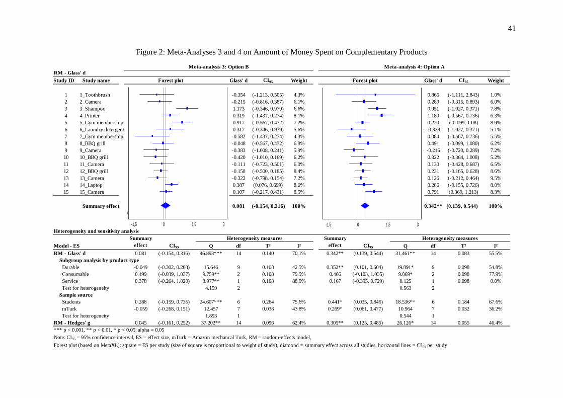
41

Figure 2: Meta-Analyses 3 and 4 on Amount of Money Spent on Complementary Products

RM - Glass' d

Study ID Study name Forest plot Glass' d CI95 Weight Forest plot Glass' d CI95 Weight

1 1_Toothbrush -0.354 (-1.213, 0.505) 4.3% 0.866 (-1.111, 2.843) 1.0%

2 2_Camera -0.215 (-0.816, 0.387) 6.1% 0.289 (-0.315, 0.893) 6.0%

3 3_Shampoo 1.173 (-0.346, 0.979) 6.6% 0.951 (-1.027, 0.371) 7.8%

4 4_Printer 0.319 (-1.437, 0.274) 8.1% 1.180 (-0.567, 0.736) 6.3%

5 5_Gym membership 0.917 (-0.567, 0.472) 7.2% 0.220 (-0.099, 1.08) 8.9%

6 6_Laundry detergent 0.317 (-0.346, 0.979) 5.6% -0.328 (-1.027, 0.371) 5.1%

7 7_Gym membership -0.582 (-1.437, 0.274) 4.3% 0.084 (-0.567, 0.736) 5.5%

8 8_BBQ grill -0.048 (-0.567, 0.472) 6.8% 0.491 (-0.099, 1.080) 6.2%

9 9_Camera -0.383 (-1.008, 0.241) 5.9% -0.216 (-0.720, 0.289) 7.2%

10 10_BBQ grill -0.420 (-1.010, 0.169) 6.2% 0.322 (-0.364, 1.008) 5.2%

11 11_Camera -0.111 (-0.723, 0.501) 6.0% 0.130 (-0.428, 0.687) 6.5%

12 12_BBQ grill -0.158 (-0.500, 0.185) 8.4% 0.231 (-0.165, 0.628) 8.6%

13 13_Camera -0.322 (-0.798, 0.154) 7.2% 0.126 (-0.212, 0.464) 9.5%

14 14_Laptop 0.387 (0.076, 0.699) 8.6% 0.286 (-0.155, 0.726) 8.0%

15 15_Camera 0.107 (-0.217, 0.431) 8.5% 0.791 (0.369, 1.213) 8.3%

Summary effect 0.081 (-0.154, 0.316) 100% 0.342** (0.139, 0.544) 100%

Heterogeneity and sensitivity analysis

Summary Summary

Model - ES effect CI95 Q df T² I² effect CI95 Q df T² I²

RM - Glass' d 0.081 (-0.154, 0.316) 46.893*** 14 0.140 70.1% 0.342** (0.139, 0.544) 31.461** 14 0.083 55.5%

Subgroup analysis by product type

Durable -0.049 (-0.302, 0.203) 15.646 9 0.108 42.5% 0.352** (0.101, 0.604) 19.891* 9 0.098 54.8%

Consumable 0.499 (-0.039, 1.037) 9.759** 2 0.108 79.5% 0.466 (-0.103, 1.035) 9.069* 2 0.098 77.9%

Service 0.378 (-0.264, 1.020) 8.977** 1 0.108 88.9% 0.167 (-0.395, 0.729) 0.125 1 0.098 0.0%

Test for heterogeneity 4.159 2 0.563 2

Sample source

Students 0.288 (-0.159, 0.735) 24.607*** 6 0.264 75.6% 0.441* (0.035, 0.846) 18.536** 6 0.184 67.6%

mTurk -0.059 (-0.268, 0.151) 12.457 7 0.038 43.8% 0.269* (0.061, 0.477) 10.964 7 0.032 36.2%

Test for heterogeneity 1.893 1 0.544 1

RM - Hedges' g 0.045 (-0.161, 0.252) 37.202** 14 0.096 62.4% 0.305** (0.125, 0.485) 26.126* 14 0.055 46.4%

*** p < 0.001, ** p < 0.01, * p < 0.05; alpha = 0.05

Note: CI95 = 95% confidence interval, ES = effect size, mTurk = Amazon mechancal Turk, RM = random-effects model,

Forest plot (based on MetaXL): square = ES per study (size of square is proportional to weight of study), diamond = summary effect across all studies, horizontal lines = CI 95 per study

Meta-analysis 3: Option B Meta-analysis 4: Option A

Heterogeneity measures Heterogeneity measures

MA3 Glass' d RM

delta31,50-1,5

Study

7_Gym membership

10_BBQ-Grill

9_Camera

1_Toothbrush

13_Camera

2_Camera

12_BBQ-Grill

11_Camera

8_BBQ-Grill

Overall

Q=46,89, p=0,00, I2=70%

15_Camera

6_Laundry detergent

4_Printer

14_Laptop

5_Gym membership

3_Shampoo

delta (95% CI) % Weight

-0,58 ( -1,44, 0,27) 4,3

-0,42 ( -1,01, 0,17) 6,2

-0,38 ( -1,01, 0,24) 5,9

-0,35 ( -1,21, 0,50) 4,3

-0,32 ( -0,80, 0,15) 7,2

-0,21 ( -0,82, 0,39) 6,1

-0,16 ( -0,50, 0,18) 8,4

-0,11 ( -0,72, 0,50) 6,0

-0,05 ( -0,57, 0,47) 6,8

0,08 ( -0,15, 0,32) 100,0

0,11 ( -0,22, 0,43) 8,5

0,32 ( -0,35, 0,98) 5,6

0,32 ( -0,05, 0,69) 8,1

0,39 ( 0,08, 0,70) 8,6

0,92 ( 0,44, 1,40) 7,2

1,17 ( 0,63, 1,71) 6,6

MA4 Glass' d RM

delta31,50-1,5

Study

6_Laundry detergent

9_Camera

7_Gym membership

13_Camera

11_Camera

5_Gym membership

12_BBQ-Grill

14_Laptop

2_Camera

10_BBQ-Grill

Overall

Q=31,46, p=0,00, I2=55%

8_BBQ-Grill

15_Camera

1_Toothbrush

3_Shampoo

4_Printer

delta (95% CI) % Weight

-0,33 ( -1,03, 0,37) 5,1

-0,22 ( -0,72, 0,29) 7,2

0,08 ( -0,57, 0,74) 5,5

0,13 ( -0,21, 0,46) 9,5

0,13 ( -0,43, 0,69) 6,5

0,22 ( -0,16, 0,60) 8,9

0,23 ( -0,17, 0,63) 8,6

0,29 ( -0,16, 0,73) 8,0

0,29 ( -0,32, 0,89) 6,0

0,32 ( -0,36, 1,01) 5,2

0,34 ( 0,14, 0,54) 100,0

0,49 ( -0,10, 1,08) 6,2

0,79 ( 0,37, 1,21) 8,3

0,87 ( -1,11, 2,84) 1,0

0,95 ( 0,49, 1,41) 7,8

1,18 ( 0,60, 1,76) 6,3

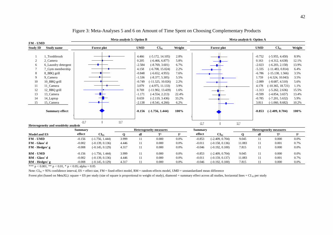
42

Figure 3: Meta-Analyses 5 and 6 on Amount of Time Spent on Choosing Complementary Products

FM - UMD

Study ID Study name Forest plot UMD CI95 Weight Forest plot UMD CI95 Weight

1 1_Toothbrush 4.466 (-5.172, 14.105) 2.8% -0.752 (-5.955, 4.450) 8.9%

2 2_Camera 0.205 (-6.466, 6.877) 5.8% 0.163 (-4.312, 4.638) 12.1%

6 6_Laundry detergent -2.584 (-8.769, 3.601) 6.7% -2.023 (-6.203, 2.158) 13.9%

7 7_Gym membership 4.158 (-6.708, 15.024) 2.2% -5.335 (-11.483, 0.814) 6.4%

8 8_BBQ grill -0.848 (-6.652, 4.955) 7.6% -6.786 (-15.138, 1.566) 3.5%

9 9_Camera -1.536 (-8.377, 5.305) 5.5% 1.759 (-6.524, 10.043) 3.5%

10 10_BBQ grill -0.749 (-11.525, 10.026) 2.2% -2.089 (-8.687, 4.510) 5.6%

11 11_Camera 3.079 (-4.975, 11.133) 3.9% 4.178 (-10.365, 18.721) 1.1%

12 12_BBQ grill 0.769 (-11.902, 13.439) 1.6% -1.313 (-5.262, 2.636) 15.5%

13 13_Camera -1.171 (-4.554, 2.213) 22.4% -0.599 (-4.854, 3.657) 13.4%

14 14_Laptop 0.659 (-2.119, 3.436) 33.2% -0.785 (-7.201, 5.632) 5.9%

15 15_Camera -2.138 (-8.541, 4.266) 6.2% 3.811 (-1.060, 8.682) 10.2%

Summary effect -0.156 (-1.756, 1.444) 100% -0.853 (-2.409, 0.704) 100%

Heterogeneity and sensitivity analysis

Summary Summary

Model and ES effect CI95 Q df T² I² effect CI95 Q df T² I²

FM - UMD -0.156 (-1.756, 1.444) 3.999 11 0.000 0.0% -0.853 (-2.409, 0.704) 9.045 11 0.000 0.0%

FM - Glass' d -0.002 (-0.139, 0.136) 4.446 11 0.000 0.0% -0.011 (-0.158, 0.136) 11.083 11 0.001 0.7%

FM - Hedges' g -0.008 (-0.145, 0.129) 4.317 11 0.000 0.0% -0.046 (-0.192, 0.100) 7.815 11 0.000 0.0%

RM - UMD -0.156 (-1.756, 1.444) 3.999 11 0.000 0.0% -0.853 (-2.409, 0.704) 9.045 11 0.000 0.0%

RM - Glass' d -0.002 (-0.139, 0.136) 4.446 11 0.000 0.0% -0.011 (-0.159, 0.137) 11.083 11 0.001 0.7%

RM - Hedges' g -0.008 (-0.145, 0.129) 4.317 11 0.000 0.0% -0.046 (-0.192, 0.100) 7.815 11 0.000 0.0%

*** p < 0.001, ** p < 0.01, * p < 0.05; alpha = 0.05

Note: CI95 = 95% confidence interval, ES = effect size, FM = fixed-effect model, RM = random-effects model, UMD = unstandardized mean difference

Forest plot (based on MetaXL): square = ES per study (size of square is proportional to weight of study), diamond = summary effect across all studies, horizontal lines = CI 95 per study

Meta-analysis 5: Option B Meta-analysis 6: Option A

Heterogeneity measures Heterogeneity measures

MA6 UMD FM

WMD11,70-11,7

Study

8_BBQ-Grill

7_Gym membership

10_BBQ-Grill

6_Laundry detergent

12_BBQ-Grill

Overall

Q=9,04, p=0,62, I2=0%

14_Laptop

1_Toothbrush

13_Camera

2_Camera

9_Camera

15_Camera

11_Camera

WMD (95% CI) % Weight

-6,79 (-15,14, 1,57) 3,5

-5,33 (-11,48, 0,81) 6,4

-2,09 ( -8,69, 4,51) 5,6

-2,02 ( -6,20, 2,16) 13,9

-1,31 ( -5,26, 2,64) 15,5

-0,85 ( -2,41, 0,70) 100,0

-0,78 ( -7,20, 5,63) 5,9

-0,75 ( -5,95, 4,45) 8,9

-0,60 ( -4,85, 3,66) 13,4

0,16 ( -4,31, 4,64) 12,1

1,76 ( -6,52, 10,04) 3,5

3,81 ( -1,06, 8,68) 10,2

4,18 (-10,36, 18,72) 1,1

MA5 UMD FM

WMD11,70-11,7

Study

6_Laundry detergent

15_Camera

9_Camera

13_Camera

8_BBQ-Grill

10_BBQ-Grill

Overall

Q=4,00, p=0,97, I2=0%

2_Camera

14_Laptop

12_BBQ-Grill

11_Camera

7_Gym membership

1_Toothbrush

WMD (95% CI) % Weight

-2,58 ( -8,77, 3,60) 6,7

-2,14 ( -8,54, 4,27) 6,2

-1,54 ( -8,38, 5,30) 5,5

-1,17 ( -4,55, 2,21) 22,4

-0,85 ( -6,65, 4,96) 7,6

-0,75 (-11,52, 10,03) 2,2

-0,16 ( -1,76, 1,44) 100,0

0,21 ( -6,47, 6,88) 5,8

0,66 ( -2,12, 3,44) 33,2

0,77 (-11,90, 13,44) 1,6

3,08 ( -4,97, 11,13) 3,9

4,16 ( -6,71, 15,02) 2,2

4,47 ( -5,17, 14,10) 2,8

43

Figure 4: Meta-Analyses 7 and 8 on the Satisfaction with the Compromise Choice

FM - UMD RM - UMD

Study ID Study name Forest plot UMD CI95 Weight Forest plot UMD CI95 Weight

1 1_Toothbrush -0.143 (-0.793, 0.508) 2.6% -0.429 (-2.561, 1.704) 0.3%

2 2_Camera -0.136 (-0.536, 0.263) 7.0% 0.141 (-0.324, 0.605) 6.8%

6 6_Laundry detergent -0.181 (-0.738, 0.375) 3.6% 0.267 (-0.206, 0.741) 6.6%

7 7_Gym membership 0.139 (-0.550, 0.828) 2.4% -0.300 (-0.873, 0.274) 4.6%

8 8_BBQ grill -0.486 (-0.987, 0.014) 4.5% -0.428 (-0.954, 0.099) 5.4%

9 9_Camera -0.597 (-1.229, 0.034) 2.8% -0.539 (-0.978, -0.099) 7.6%

10 10_BBQ grill -0.135 (-0.543, 0.274) 6.7% 0.034 (-0.664, 0.733) 3.1%

11 11_Camera -0.361 (-0.817, 0.095) 5.4% 0.006 (-0.489, 0.502) 6.1%

12 12_BBQ grill -0.396 (-0.638, -0.155) 19.2% -0.284 (-0.574, 0.006) 15.9%

13 13_Camera -0.482 (-0.870, -0.093) 7.4% -0.093 (-0.358, 0.173) 18.5%

14 14_Laptop -0.202 (-0.434, 0.030) 20.8% -0.281 (-0.658, 0.096) 10.0%

15 15_Camera -0.073 (-0.325, 0.179) 17.6% 0.001 (-0.300, 0.301) 15.0%

Summary effect -0.250*** (-0.356, -0.144) 100% -0.141* (-0.267, -0.015) 100%

Heterogeneity and sensitivity analysis

Summary Summary

Model and ES effect CI95 Q df T² I² effect CI95 Q df T² I²

FM - UMD -0.250*** (-0.356, -0.144) 9.095 11 0.000 0.0%

FM - Glass' d -0.339*** (-0.478, -0.199) 10.844 11 0.000 0.0%

RM - UMD -0.250*** (-0.356, -0.144) 9.095 11 0.000 0.0% -0.141* (-0.267, -0.015) 11.951 11 0.004 8.0%

RM - Glass' d -0.190* (-0.352, -0.029) 12.620 11 0.010 12.8%

*** p < 0.001, ** p < 0.01, * p < 0.05; alpha = 0.05

Note: CI95 = 95% confidence interval, ES = effect size, FM = fixed-effectts model, RM = random-effects model, UMD = unstandardized mean difference

Forest plot (based on MetaXL): squares = ES per study (size of square is proportional to weight per study), diamond = summary effect across all studies, horizontal lines = CI 95 per study

Meta-analysis 7: Option B Meta-analysis 8: Option A

Heterogeneity measures Heterogeneity measures

MA8 UMD RM

WMD10-1-2

Study

9_Camera

1_Toothbrush

8_BBQ-Grill

7_Gym membership

12_BBQ-Grill

14_Laptop

Overall

Q=11,95, p=0,37, I2=8%

13_Camera

15_Camera

11_Camera

10_BBQ-Grill

2_Camera

6_Laundry detergent

WMD (95% CI) % Weight

-0,54 ( -0,98, -0,10) 7,6

-0,43 ( -2,56, 1,70) 0,3

-0,43 ( -0,95, 0,10) 5,4

-0,30 ( -0,87, 0,27) 4,6

-0,28 ( -0,57, 0,01) 15,9

-0,28 ( -0,66, 0,10) 10,0

-0,14 ( -0,27, -0,02) 100,0

-0,09 ( -0,36, 0,17) 18,5

0,00 ( -0,30, 0,30) 15,0

0,01 ( -0,49, 0,50) 6,1

0,03 ( -0,66, 0,73) 3,1

0,14 ( -0,32, 0,61) 6,8

0,27 ( -0,21, 0,74) 6,6

MA7 UMD FM

WMD0-1

Study

9_Camera

8_BBQ-Grill

13_Camera

12_BBQ-Grill

11_Camera

Overall

Q=9,09, p=0,61, I2=0%

14_Laptop

6_Laundry detergent

1_Toothbrush

2_Camera

10_BBQ-Grill

15_Camera

7_Gym membership

WMD (95% CI) % Weight

-0,60 ( -1,23, 0,03) 2,8

-0,49 ( -0,99, 0,01) 4,5

-0,48 ( -0,87, -0,09) 7,4

-0,40 ( -0,64, -0,16) 19,2

-0,36 ( -0,82, 0,09) 5,4

-0,25 ( -0,36, -0,14) 100,0

-0,20 ( -0,43, 0,03) 20,8

-0,18 ( -0,74, 0,37) 3,6

-0,14 ( -0,79, 0,51) 2,6

-0,14 ( -0,54, 0,26) 7,0

-0,13 ( -0,54, 0,27) 6,7

-0,07 ( -0,32, 0,18) 17,6

0,14 ( -0,55, 0,83) 2,4

44

Figure 5: Meta-Analyses 9 and 10 on the Confidence in the Compromise Choice

RM - UMD

Study ID Study name Forest plot UMD CI95 Weight Forest plot UMD CI95 Weight

1 1_Toothbrush -0.500 (-1.732, 0.732) 1.4% -0.929 (-2.219, 0.362) 1.2%

2 2_Camera -0.463 (-0.974, 0.047) 6.8% -0.277 (-0.662, 0.108) 10.7%

6 6_Laundry detergent -0.123 (-0.826, 0.580) 3.9% -0.059 (-0.604, 0.487) 6.0%

7 7_Gym membership 0.153 (-0.549, 0.854) 3.9% -0.518 (-0.946, -0.090) 9.1%

8 8_BBQ grill -0.420 (-0.913, 0.073) 7.2% -0.181 (-0.735, 0.373) 5.8%

9 9_Camera -0.944 (-1.437, -0.452) 7.2% -0.461 (-0.987, 0.064) 6.4%

10 10_BBQ grill 0.048 (-0.431, 0.527) 7.5% -0.756 (-1.180, -0.331) 9.2%

11 11_Camera -0.417 (-0.906, 0.072) 7.2% 0.072 (-0.596, 0.741) 4.2%

12 12_BBQ grill -0.396 (-0.690, -0.101) 14.8% -0.586 (-0.920, -0.251) 13.3%

13 13_Camera -0.701 (-1.154, -0.248) 8.2% -0.289 (-0.591, 0.013) 15.3%

14 14_Laptop -0.358 (-0.672, -0.045) 13.7% -0.196 (-0.646, 0.254) 8.3%

15 15_Camera -0.218 (-0.462, 0.025) 18.2% -0.031 (-0.418, 0.356) 10.6%

Summary effect -0.366*** (-0.513, -0.219) 100% -0.339*** (-0.481, -0.197) 100%

Heterogeneity and sensitivity analysis

Summary Summary

Model - ES effect CI95 Q df T² I² effect CI95 Q df T² I²

RM - UMD -0.366*** (-0.513, -0.219) 14.532 11 0.015 24.3% -0.339*** (-0.481, -0.197) 13.284 11 0.011 17.2%

RM - Glass' d -0.435*** (-0.610, -0.260) 15.015 11 0.024 26.7% -0.372*** (-0.569, -0.174) 17.079 11 0.040 35.6%

*** p < 0.001, ** p < 0.01, * p < 0.05; alpha = 0.05

Note: CI95 = 95% confidence interval, ES = effect size, RM = random-effects model, UMD = unstandardized mean difference

Forest plot (based on MetaXL): squares = ES per study (size of square is proportional to weight per study), diamond = summary effect across all studies, horizontal lines = CI 95 per study

Meta-analysis 9: Option B Meta-analysis 10: Option A

Heterogeneity measures Heterogeneity measures

MA10 UMD RM

WMD0,70-0,7-1,4-2,1

Study

1_Toothbrush

10_BBQ-Grill

12_BBQ-Grill

7_Gym membership

9_Camera

Overall

Q=13,28, p=0,28, I2=17%

13_Camera

2_Camera

14_Laptop

8_BBQ-Grill

6_Laundry detergent

15_Camera

11_Camera

WMD (95% CI) % Weight

-0,93 ( -2,22, 0,36) 1,2

-0,76 ( -1,18, -0,33) 9,2

-0,59 ( -0,92, -0,25) 13,3

-0,52 ( -0,95, -0,09) 9,1

-0,46 ( -0,99, 0,06) 6,4

-0,34 ( -0,48, -0,20) 100,0

-0,29 ( -0,59, 0,01) 15,3

-0,28 ( -0,66, 0,11) 10,7

-0,20 ( -0,65, 0,25) 8,3

-0,18 ( -0,74, 0,37) 5,8

-0,06 ( -0,60, 0,49) 6,0

-0,03 ( -0,42, 0,36) 10,6

0,07 ( -0,60, 0,74) 4,2

MA9 UMD RM

WMD0,70-0,7-1,4-2,1

Study

9_Camera

13_Camera

1_Toothbrush

2_Camera

8_BBQ-Grill

11_Camera

12_BBQ-Grill

Overall

Q=14,53, p=0,20, I2=24%

14_Laptop

15_Camera

6_Laundry detergent

10_BBQ-Grill

7_Gym membership

WMD (95% CI) % Weight

-0,94 ( -1,44, -0,45) 7,2

-0,70 ( -1,15, -0,25) 8,2

-0,50 ( -1,73, 0,73) 1,4

-0,46 ( -0,97, 0,05) 6,8

-0,42 ( -0,91, 0,07) 7,2

-0,42 ( -0,91, 0,07) 7,2

-0,40 ( -0,69, -0,10) 14,8

-0,37 ( -0,51, -0,22) 100,0

-0,36 ( -0,67, -0,04) 13,7

-0,22 ( -0,46, 0,03) 18,2

-0,12 ( -0,83, 0,58) 3,9

0,05 ( -0,43, 0,53) 7,5

0,15 ( -0,55, 0,85) 3,9

45

Figure 6: Meta-Analyses 11 and 12 on the Difficulty of the Compromise Choice

RM - UMD

Study ID Study name Forest plot UMD CI95 Weight Forest plot UMD CI95 Weight

1 1_Toothbrush 0.667 (-0.647, 1.980) 2.6% 1.571 (0.731, 2.411) 4.4%

2 2_Camera 0.515 (-0.013, 1.044) 9.2% 0.424 (-0.169, 1.018) 7.7%

6 6_Laundry detergent -0.029 (-0.901, 0.842) 5.0% 0.139 (-0.748, 1.026) 4.0%

7 7_Gym membership -1.243 (-2.014, -0.473) 5.9% 0.745 (0.002, 1.489) 5.4%

8 8_BBQ grill 0.390 (-0.198, 0.978) 8.2% -0.167 (-0.737, 0.404) 8.2%

9 9_Camera 0.861 (0.064, 1.658) 5.6% -0.072 (-0.708, 0.564) 7.0%

10 10_BBQ grill 0.095 (-0.488, 0.677) 8.3% 0.353 (-0.184, 0.891) 8.9%

11 11_Camera 0.097 (-0.518, 0.713) 7.8% 0.219 (-0.426, 0.864) 6.8%

12 12_BBQ grill 0.195 (-0.135, 0.525) 13.2% 0.521 (0.104, 0.938) 12.4%

13 13_Camera -0.053 (-0.622, 0.516) 8.5% 0.241 (-0.142, 0.623) 13.6%

14 14_Laptop 0.459 (0.117, 0.802) 12.9% 0.378 (-0.098, 0.853) 10.5%

15 15_Camera 0.378 (0.018, 0.738) 12.6% 0.375 (-0.088, 0.837) 10.9%

Summary effect 0.214 (-0.014, 0.442) 100% 0.355*** (0.163, 0.546) 100%

Heterogeneity and sensitivity analysis

Summary Summary

Model and ES effect CI95 Q df T² I² effect CI95 Q df T² I²

RM - UMD 0.214 (-0.014, 0.442) 22.281* 11 0.074 50.6% 0.355*** (0.163, 0.546) 15.468 11 0.032 28.9%

RM - Glass' d 0.229* (0.034, 0.425) 18.952 11 0.046 42.0% 0.275*** (0.127, 0.424) 9.762 11 0.000 0.0%

*** p < 0.001, ** p < 0.01, * p < 0.05; alpha = 0.05

Note: CI95 = 95% confidence interval, ES = effect size, RM = random-effects model, UMD = unstandardized mean difference

Forest plot (based on MetaXL): squares = ES per study (size of square is proportional to weight per study), diamond = summary effect across all studies, horizontal lines = CI 95 per study

Meta-analysis 11: Option B Meta-analysis 12: Option A

Heterogeneity measures Heterogeneity measures

MA11 UMD RM

WMD1,80,90-0,9-1,8

Study

7_Gym membership

13_Camera

6_Laundry detergent

10_BBQ-Grill

11_Camera

12_BBQ-Grill

Overall

Q=22,28, p=0,02, I2=51%

15_Camera

8_BBQ-Grill

14_Laptop

2_Camera

1_Toothbrush

9_Camera

WMD (95% CI) % Weight

-1,24 ( -2,01, -0,47) 5,9

-0,05 ( -0,62, 0,52) 8,5

-0,03 ( -0,90, 0,84) 5,0

0,09 ( -0,49, 0,68) 8,3

0,10 ( -0,52, 0,71) 7,8

0,19 ( -0,14, 0,53) 13,2

0,21 ( -0,01, 0,44) 100,0

0,38 ( 0,02, 0,74) 12,6

0,39 ( -0,20, 0,98) 8,2

0,46 ( 0,12, 0,80) 12,9

0,52 ( -0,01, 1,04) 9,2

0,67 ( -0,65, 1,98) 2,6

0,86 ( 0,06, 1,66) 5,6

MA12 UMD RM

WMD1,80,90-0,9-1,8

Study

8_BBQ-Grill

9_Camera

6_Laundry detergent

11_Camera

13_Camera

10_BBQ-Grill

Overall

Q=15,47, p=0,16, I2=29%

15_Camera

14_Laptop

2_Camera

12_BBQ-Grill

7_Gym membership

1_Toothbrush

WMD (95% CI) % Weight

-0,17 ( -0,74, 0,40) 8,2

-0,07 ( -0,71, 0,56) 7,0

0,14 ( -0,75, 1,03) 4,0

0,22 ( -0,43, 0,86) 6,8

0,24 ( -0,14, 0,62) 13,6

0,35 ( -0,18, 0,89) 8,9

0,35 ( 0,16, 0,55) 100,0

0,37 ( -0,09, 0,84) 10,9

0,38 ( -0,10, 0,85) 10,5

0,42 ( -0,17, 1,02) 7,7

0,52 ( 0,10, 0,94) 12,4

0,75 ( 0,00, 1,49) 5,4

1,57 ( 0,73, 2,41) 4,4

46

Figure 7: Meta-Analyses 13 to 18 on Evaluation of the Choice of Complementary Products

Model

FM - UMD

ID Study name Forest plot UMD CI95 Weight Forest plot UMD CI95 Weight

10 10_BBQ grill -0.046 (-0.555, 0.462) 5.2% -0.480 (-1.025, 0.065) 6.1%

11 11_Camera -0.431 (-0.957, 0.096) 4.8% -0.116 (-0.492, 0.260) 12.9%

12 12_BBQ grill -0.178 (-0.401, 0.044) 27.0% -0.377 (-0.669, -0.084) 21.2%

13 13_Camera -0.215 (-0.544, 0.115) 12.3% -0.122 (-0.382, 0.138) 26.9%

14 14_Laptop -0.122 (-0.348, 0.105) 26.1% 0.092 (-0.294, 0.477) 12.2%

15 15_Camera -0.008 (-0.241, 0.225) 24.6% -0.021 (-0.317, 0.276) 20.7%

Summary effect -0.131* (-0.247, -0.016) 100% -0.150* (-0.285, -0.015) 100%

Heterogeneity Q = 2.849, T² = 0.000, I² = 0.0% Q = 6.025 , T² = 0.006, I² = 17.0%

FM - Hedges' g

Summary effect -0.179* (-0.340, -0.019) -0.184* (-0.360, -0.008)

Heterogeneity Q = 2.740, T² = 0.000, I² = 0.0% Q = 6.025, T² = 0.011, I² = 17.4%

Model

FM - UMD

ID Study name Forest plot UMD CI95 Weight Forest plot UMD CI95 Weight

10 10_BBQ grill -0.300 (-0.724, 0.125) 7.6% -0.618 (-1.226, -0.010) 5.4%

11 11_Camera -0.208 (-0.594, 0.178) 9.2% -0.055 (-0.554, 0.445) 8.0%

12 12_BBQ grill -0.136 (-0.385, 0.114) 21.9% -0.513 (-0.817, -0.209) 21.5%

13 13_Camera -0.181 (-0.571, 0.209) 9.0% -0.222 (-0.492, 0.048) 27.3%

14 14_Laptop -0.202 (-0.415, 0.010) 30.2% -0.121 (-0.518, 0.275) 12.6%

15 15_Camera -0.035 (-0.283, 0.213) 22.1% -0.161 (-0.442, 0.120) 25.2%

Summary effect -0.157** (-0.273, -0.040) 100% -0.265***(-0.406, -0.123) 100%

Heterogeneity Q = 1.645, T² = 0.000, I² = 0.0% Q = 5.667 , T² = 0.004, I² = 11.8%

FM - Hedges' g

Summary effect -0.209* (-0.370, -0.048) -0.318***(-0.495, -0.142)

Heterogeneity Q = 1.827, T² = 0.000, I² = 0.0% Q = 5.575, T² = 0.006, I² = 10.3%

Model

FM - UMD

ID Study name Forest plot UMD CI95 Weight Forest plot UMD CI95 Weight

10 10_BBQ grill 0.069 (-0.578, 0.716) 7.2% 0.678 (0.104, 1.252) 10.1%

11 11_Camera 0.319 (-0.359, 0.998) 6.5% -0.129 (-0.809, 0.551) 7.2%

12 12_BBQ grill 0.201 (-0.148, 0.551) 24.7% 0.441 (0.076, 0.807) 25.0%

13 13_Camera -0.263 (-0.776, 0.251) 11.4% 0.152 (-0.230, 0.534) 22.9%

14 14_Laptop 0.174 (-0.156, 0.503) 27.8% 0.179 (-0.315, 0.674) 13.6%15 15_Camera -0.004 (-0.372, 0.364) 22.3% 0.435 (0.038, 0.832) 21.2%

Summary effect 0.093 (-0.081, 0.267) 100% 0.321** (0.138, 0.504) 100%

Heterogeneity Q = 3.145, T² = 0.000, I² = 0.0% Q = 4.972 , T² = 0.000, I² = 0.0%

FM - Glass' d

Summary effect 0.088 (-0.073, 0.249) 0.307** (0.128, 0.487)

Heterogeneity Q = 3.262, T² = 0.000, I² = 0.0% Q = 7.251, T² = 0.023, I² = 31.0%

*** p < 0.001, ** p < 0.01, * p < 0.05; alpha = 0.05

Note: CI95 = 95% confidence interval, ES = effect size, FM = fixed-effects model, UMD = unstandardized mean difference

Forest plots (based on Excel): dots = ES per study (size of dot independent of weight of per study), horizontal lines = CI95 per study

Meta-analysis 17: Option B Meta-analysis 18: Option A

Meta-analyses on satisfaction with choice of complementary products

Meta-analyses on confidence in choice of complementary products

Meta-analyses on difficulty of choice of complementary products

Meta-analysis 13: Option B Meta-analysis 14: Option A

Meta-analysis 15: Option B Meta-analysis 16: Option A

-1.2 -0.2-1.2 -0.2

-1.3 -0.8 -0.3 0.2-1.3 -0.8 -0.3 0.2

-0.9 1.2 -0.9 1.2

47

Appendix

Author/s (Year)

[Journal]

Research Focus Theoretical

Background

Sample Method/Analysis Main Findings

Aguinis et al.

(2011)

[Journal of

Management]

Impact of the

method of the

meta-analysis and

judgement calls on

the magnitude of

the effect size of

the meta-analysis

Methodological

foundation of

meta-analysis

196 meta-analyses

from the time-

period 1982-2009

with 5581 effect

sizes

• 21 different

meta-analysis

methods

ANCOVA

• IV:

methodological

choices,

judgment calls

• DV: absolute-

value meta-

analytical

derived effect

sizes

• Choice of meta-analysis method

and judgement calls have a small

influence on the conclusion of

the analysis and the effect size

• Methodological choices and

judgement calls are linked to the

number of citations of the

respective analysis

• Increased magnitude of the effect

sizes does not result in a higher

citation rate

• If a meta-analysis tests existing

theory, the number of citation

increases

• If a meta-analysis tries to create

new theory, the number of

citations decreases

48

Author/s (Year)

[Journal]

Research Focus Theoretical

Background

Sample Method/Analysis Main Findings

Churchill Jr. and

Peter (1984)

[Journal of

Marketing

Research]

Impact of research

design effects on

the reliability of

rating scales

• Measurement

theory

• Psychometric

theory

101 studies

including

information on

reliability leading

to a total of 154

measures

Meta-analysis

IV:

• Sampling

characteristics

• Measure

characteristics

• Measure

development

processes

DV:

• Reliability

coefficient

Regression

analysis

• The influence of following

research design characteristics

are investigated: sampling and

measure characteristics and

measure development processes

• The measure characteristics have

a strong impact on the reliability

estimates

• The characteristics of measures

account for 22% of variance in

the estimate of reliability

Sampling characteristics and

measure development processes

have a very small influence

49

Author/s (Year)

[Journal]

Research Focus Theoretical

Background

Sample Method/Analysis Main Findings

Cochran (1954)

[Biometrics]

Mathematical

theory and

discussion of

methods regarding

the combination of

estimates from

different

experiments

- - Mathematical

models

• Derivation and presentation of

methods regarding the estimates

from different experiments

• The simplest estimator is the

arithmetic mean of the estimates

• Unweighted mean is the best

estimator in case of experiments

which are of the same type

• The best estimator across

experiments is the weighted

mean if the variance per

observation is the same and the

experiments differ

• The presence of interactions

impacts the choice of the

estimator

• The estimator of the unweighted

mean fits most settings in

practice

50

Author/s (Year)

[Journal]

Research Focus Theoretical

Background

Sample Method/Analysis Main Findings

DerSimonian and

Laird (1986)

[Clinical Trials]

Consistent

assessment of

homogeneity of

treatment effect

Methodological

foundation of

meta-analysis:

random-effects

model

n = 8 published

reviews

Random-effects

model

• Discussion of a random-effects

method that examines the

heterogeneity regarding the

overall effect

• Heterogeneity is an important

indicator to be assessed during

the analysis

• Derivation of an estimator of the

amount of heterogeneity

• A weighted noniterative

approach is a suggested approach

to estimate the total effect of the

treatment and its variation in the

effect over all studies Analysis of

further influencing factors that

have an impact on heterogeneity

is included in this method

51

Author/s (Year)

[Journal]

Research Focus Theoretical

Background

Sample Method/Analysis Main Findings

Dhar and

Simonson (2003)

[Journal of

Marketing

Research]

Impact of a no-

choice option on

the attraction and

compromise effect

• Forced choices

• Independence

of irrelevant

alternatives

• Compromise

effect

Study 1 :

n = 140 visitors to

a science museum

Study 2:

n = 322 visitors to

a science museum

Study 3:

n = 120

passengers to a

major airport

Study 4:

n = 110 visitors of

a science museum

Study 5:

n = 216

undergraduate

students

• Logit model

• Between-

subject design

with random

assignment

• The introduction of a no-choice

option increases the attraction

effect

• The introduction of a no-choice

option decreases the compromise

effect

• The introduction of a no-choice

option results in a decrease of the

share of the alternative, which

performances on average

regarding the dimensions in

comparison to the no-choice

option

• The proportion of the no-choice

option increases if attributes are

displayed in form of ranges

• The share of a no-choice option

is higher if a forced-choice takes

place beforehand

52

Author/s (Year)

[Journal]

Research Focus Theoretical

Background

Sample Method/Analysis Main Findings

Eisend (2015)

[Journal of

Marketing]

Measurement of

the created

progress and value

of knowledge in

the field of

marketing

research

• Marketing

research

• Marketing

knowledge

• Method meta-

analysis

• n = 176 meta-

analyses from

the time period

1918 to 2012

including more

than 7500

primary studies

• 1841 effect

sizes

Meta-meta-

analysis

• Main IV: time,

maturity,

intensity

• DV: effect size

• A substantial amount of

knowledge is created in

marketing which is represented

by a medium-sized mean

correlation in meta-analysis of

0.24

• The highest effects are provided

by the areas pricing and

consumer behavior

• The amount of created

knowledge varies across research

areas

• Knowledge has been created

during a long period of time with

a declining rate

• Maturity in marketing knowledge

is obvious

53

Author/s (Year)

[Journal]

Research Focus Theoretical

Background

Sample Method/Analysis Main Findings

Fern and Monroe

(1996)

[Journal of

Consumer

Research]

Challenges of the

estimation of the

effect size

Methodological

foundation of the

meta-analysis

- - • The interpretability of an effect

size depends on the nature of

research, i.e. relational vs.

experimental, the research

objective, i.e. testing of theory or

applicational focus, and the

history in this research field

• The factors, that influence the

size of the effect, need to be

considered before analyzing and

interpreting the value

• The analysis of heterogeneity is

essential in a meta-analysis

54

Author/s (Year)

[Journal]

Research Focus Theoretical

Background

Sample Method/Analysis Main Findings

Glass (1976)

[Educational

Researcher]

Introduction to the

method meta-

analysis illustrated

by example

• Educational

research

• Methodological

foundation of

the meta-

analysis

800 measured

effect sizes from

375 studies

Meta-analysis

from the field of

therapy to

illustrate the

method meta-

analysis

• Meta-analysis is defined as

analysis that examines analyses

• Condensing the information from

various studies is an essential

and difficult issue for educational

researchers

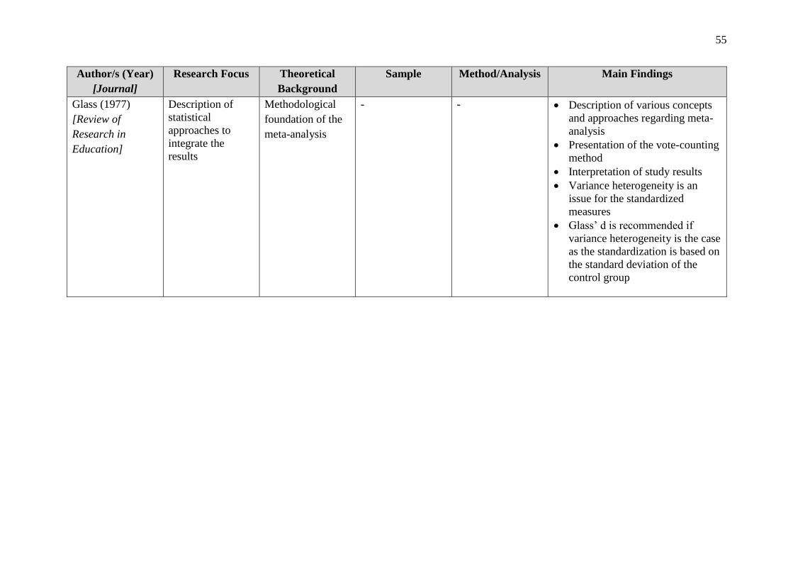
55

Author/s (Year)

[Journal]

Research Focus Theoretical

Background

Sample Method/Analysis Main Findings

Glass (1977)

[Review of

Research in

Education]

Description of

statistical

approaches to

integrate the

results

Methodological

foundation of the

meta-analysis

- - • Description of various concepts

and approaches regarding meta-

analysis

• Presentation of the vote-counting

method

• Interpretation of study results

• Variance heterogeneity is an

issue for the standardized

measures

• Glass’ d is recommended if

variance heterogeneity is the case

as the standardization is based on

the standard deviation of the

control group

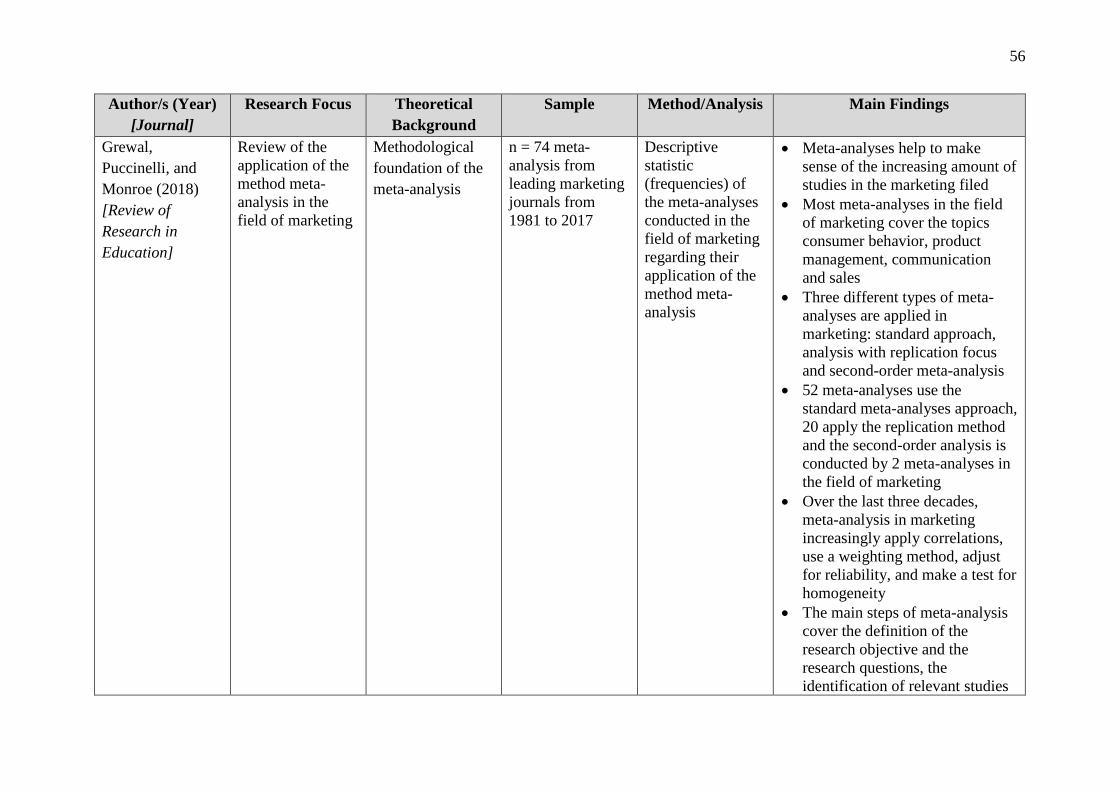
56

Author/s (Year)

[Journal]

Research Focus Theoretical

Background

Sample Method/Analysis Main Findings

Grewal,

Puccinelli, and

Monroe (2018)

[Review of

Research in

Education]

Review of the

application of the

method meta-

analysis in the

field of marketing

Methodological

foundation of the

meta-analysis

n = 74 meta-

analysis from

leading marketing

journals from

1981 to 2017

Descriptive

statistic

(frequencies) of

the meta-analyses

conducted in the

field of marketing

regarding their

application of the

method meta-

analysis

• Meta-analyses help to make

sense of the increasing amount of

studies in the marketing filed

• Most meta-analyses in the field

of marketing cover the topics

consumer behavior, product

management, communication

and sales

• Three different types of meta-

analyses are applied in

marketing: standard approach,

analysis with replication focus

and second-order meta-analysis

• 52 meta-analyses use the

standard meta-analyses approach,

20 apply the replication method

and the second-order analysis is

conducted by 2 meta-analyses in

the field of marketing

• Over the last three decades,

meta-analysis in marketing

increasingly apply correlations,

use a weighting method, adjust

for reliability, and make a test for

homogeneity

• The main steps of meta-analysis

cover the definition of the

research objective and the

research questions, the

identification of relevant studies

57

to be included, the calculation of

the effect sizes per individual

study, choice of the model to

integrate the effect sizes, a test

for homogeneity and analysis of

essential moderators

58

Author/s (Year)

[Journal]

Research Focus Theoretical

Background

Sample Method/Analysis Main Findings

Hall and Brannick

(2002)

[Journal of

Applied

Psychology]

Comparison of the

two random-

effects methods

Schmidt-Hunter

method and

Hedges-Vevea

method

Methodological

foundation of the

meta-analysis:

random-effects

model

4 meta-analyses Monte Carlo

simulation

• Manipulation

of the

population

effect, standard

deviation of

the population,

sum of studies

and the

attenuation

• Random

variable:

sample size per

study

Meta-analysis of

four published

meta-analysis

applying both

methods

• The choice of the method has a

smaller effect on the result of the

study than the procedure of the

consideration and correction of

the artefacts

• The Monte Carlo simulation

shows that the credibility interval

of the Schmidt-Hunter method is

better as the Hedges-Vevea

method tends to calculate

credibility intervals which

include zero erroneously

• The re-analysis of the four meta-

analyses using both methods only

gives indications on which

method is preferred

• If the correction regarding

reliability is not part of the

analysis, both methods calculate

very similar results

• Schmidt-Hunter-method

computes credibility intervals

which reflect reality to a better

extend

• Schmidt-Hunter-method creates

more precise estimates and

credibility intervals

59

Author/s (Year)

[Journal]

Research Focus Theoretical

Background

Sample Method/Analysis Main Findings

Hedges (1981)

[Journal of

Educational

Statistics]

Distribution

theory for Glass’s

estimator of effect

size and related

estimators

Methodological

foundation of the

meta-analysis:

effect size by

Glass

- Statistical model

• Derivation of the distribution of

the effect size of Glass

• The estimator of Glass’ effect

size is slightly biased

• Creation of a correction for the

influence of the measurement

error on the estimated effect size

• Derivation of accurate weights

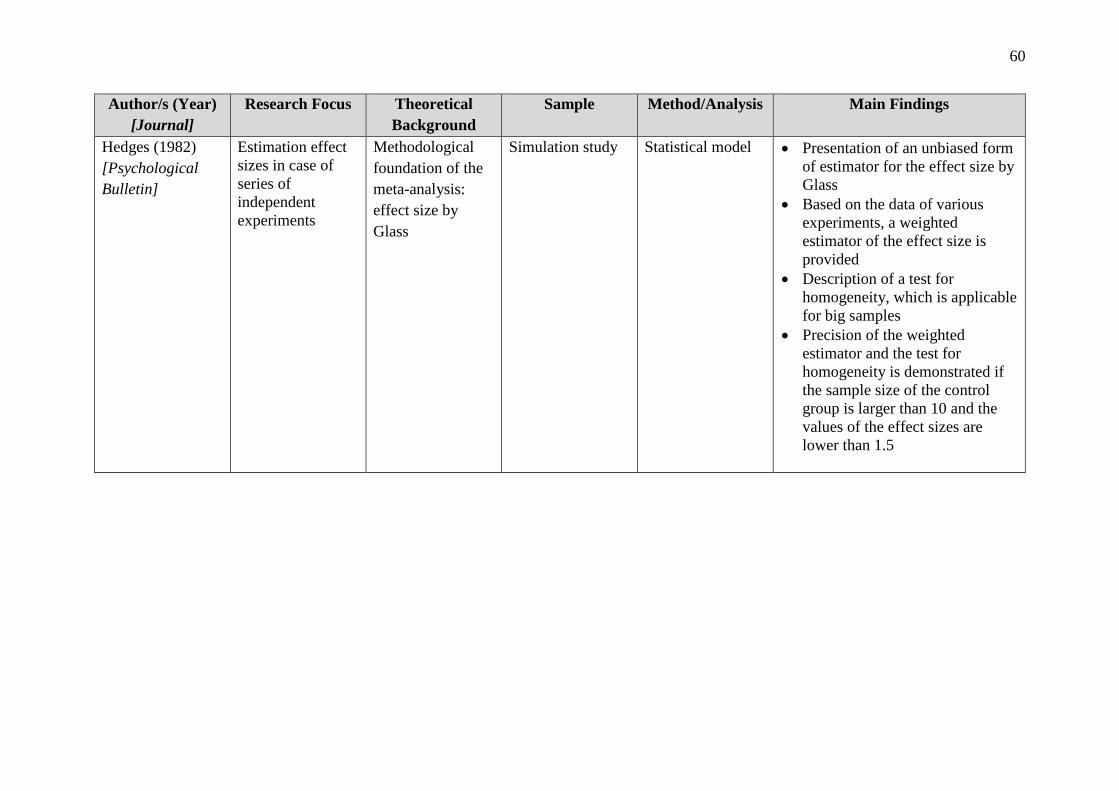
60

Author/s (Year)

[Journal]

Research Focus Theoretical

Background

Sample Method/Analysis Main Findings

Hedges (1982)

[Psychological

Bulletin]

Estimation effect

sizes in case of

series of

independent

experiments

Methodological

foundation of the

meta-analysis:

effect size by

Glass

Simulation study Statistical model

• Presentation of an unbiased form

of estimator for the effect size by

Glass

• Based on the data of various

experiments, a weighted

estimator of the effect size is

provided

• Description of a test for

homogeneity, which is applicable

for big samples

• Precision of the weighted

estimator and the test for

homogeneity is demonstrated if

the sample size of the control

group is larger than 10 and the

values of the effect sizes are

lower than 1.5

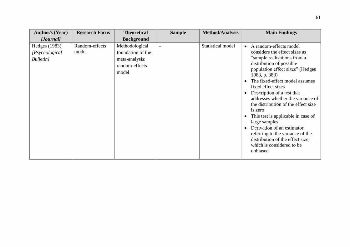
61

Author/s (Year)

[Journal]

Research Focus Theoretical

Background

Sample Method/Analysis Main Findings

Hedges (1983)

[Psychological

Bulletin]

Random-effects

model

Methodological

foundation of the

meta-analysis:

random-effects

model

- Statistical model

• A random-effects model

considers the effect sizes as

“sample realizations from a

distribution of possible

population effect sizes” (Hedges

1983, p. 388)

• The fixed-effect model assumes

fixed effect sizes

• Description of a test that

addresses whether the variance of

the distribution of the effect size

is zero

• This test is applicable in case of

large samples

• Derivation of an estimator

referring to the variance of the

distribution of the effect size,

which is considered to be

unbiased

62

Author/s (Year)

[Journal]

Research Focus Theoretical

Background

Sample Method/Analysis Main Findings

Hedges and Olkin

(1980)

[Psychological

Bulletin]

Method of vote-

counting

- - Statistical model

• The vote-counting method is

intuitive but low in power

• Vote-counting is about counting

the studies in which the mean of

the treatment group is larger than

the mean of the control group. In

case of the relative share of

studies, in which the mean of the

treatment group is greater than

the mean in the control group, is

large, the treatment is considered

to have an effect

• The power of this method further

declines if the amount of studies

included rises

• Description of further methods

like the calculation of confidence

intervals of the effect size

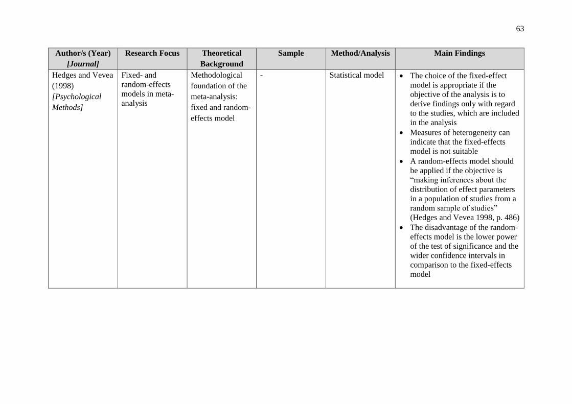
63

Author/s (Year)

[Journal]

Research Focus Theoretical

Background

Sample Method/Analysis Main Findings

Hedges and Vevea

(1998)

[Psychological

Methods]

Fixed- and

random-effects

models in meta-

analysis

Methodological

foundation of the

meta-analysis:

fixed and random-

effects model

- Statistical model

• The choice of the fixed-effect

model is appropriate if the

objective of the analysis is to

derive findings only with regard

to the studies, which are included

in the analysis

• Measures of heterogeneity can

indicate that the fixed-effects

model is not suitable

• A random-effects model should

be applied if the objective is

“making inferences about the

distribution of effect parameters

in a population of studies from a

random sample of studies”

(Hedges and Vevea 1998, p. 486)

• The disadvantage of the random-

effects model is the lower power

of the test of significance and the

wider confidence intervals in

comparison to the fixed-effects

model

64

Author/s (Year)

[Journal]

Research Focus Theoretical

Background

Sample Method/Analysis Main Findings

Higgins and

Thompson (2002)

[Statistics in

Medicine]

Measurement of

heterogeneity in

meta-analysis

Methodological

foundation of the

meta-analysis:

measurement of

heterogeneity

Exemplary studies

used for

illustration

Application of all

three

heterogeneity

measures on an

exemplary data set

• Proposition of the heterogeneity

parameter H, R and I² which are

independent of the amount of

trials included

• All three measures are

considered to be more important

than the test for homogeneity

• All three measures target the

magnitude of heterogeneity

• Description and interpretation of

these heterogeneity measures and

their intervals based on five

exemplary data sets

• H and I² are preferred over R

• H is the “ratio of confidence

interval widths for single

summary estimates” (Higgins

and Thompson 2002, p. 1553)

• I² is the share of variation due to

real differences than based on

sampling error

65

Author/s (Year)

[Journal]

Research Focus Theoretical

Background

Sample Method/Analysis Main Findings

Higgins et al.

(2003)

[British Medical

Journal]

Measurement of

inconsistency in

meta-analysis

Methodological

foundation of the

meta-analysis:

measurement of

heterogeneity

Exemplary studies

used for

illustration

Meta-analysis

with focus on

heterogeneity

measures

• Description of the heterogeneity

parameter I²

• The disadvantage of the test for

homogeneity is its dependence

on the number of studies

incorporated

• The parameter I² is independent

of the amount of trials included

in the analysis and is comparable

across various data

• I² measures the share of the “total

variation across studies due to

heterogeneity” (Higgins et al.

2003, p. 559)

• I² ranges from 0% to 100%

• It is also applicable in subgroup

analysis

• 25% is considered as low, 50%

as moderate and 75% as high

heterogeneity

66

Author/s (Year)

[Journal]

Research Focus Theoretical

Background

Sample Method/Analysis Main Findings

Johnson, Mullen,

and Salas (1995)

[Journal of

Applied

Psychology]

Comparison of

three meta-

analytic methods

Methodological

foundation of the

meta-analysis:

models of meta-

analysis

Exemplary studies

used for

illustration

Meta-analyses

based on three

distinct meta-

analysis methods

• All three models produce similar

estimates of the summary effect

and the variability of the

individual effect sizes

• In general, the model by Hedges

and Olkin leads to similar results

regarding the significance of the

summary effect or the analysis of

moderators as the approach by

Rosenthal and Rubin

• The results of the technique by

Hunter, Schmidt and Jackson

deviate from the previous

models: the significance level is

more conservative

• The model by Hunter, Schmidt

and Jackson is more complex as

it corrects for further factors like

the reliability of the dependent

variable

• The model by Hunter, Schmidt

and Jackson should be applied

carefully

67

Author/s (Year)

[Journal]

Research Focus Theoretical

Background

Sample Method/Analysis Main Findings

Kivetz, Netzer,

and Srinivasan

(2004)

[Journal of

Marketing

Research]

Integration of the

compromise

effect in

formal choice

models

• Standard value

maximization

model

• Formal choice

model

• Contextual

concavity

model

• Relative

advantage

model

• Normalized

contextual

concavity

model

• Loss-aversion

model

Empirical

application 1:

n = 1.088 travelers

waiting for their

flights at domestic

terminals in a

major airport

Empirical

application 2:

n = 205 students at

a private West

Coast University

Empirical

application 1:

• Parthworth

function

preference

model

Empirical

application 2:

• Conjoint

analysis

parthworths

• Four distinct context-dependent

choice models are tested whether

they can display the compromise

effect

• The results and the fit of the

models are better if they include

the local choice context in

contrast to the value

maximization model

• The compromise effect

systematically influences the

decision “in larger sets of

products and attributes than has

been previously shown” (Kivetz,

Netzer, and Srinivasan 2004, p.

237)

• Local concavity and loss

aversion are similar constructs

• Approaches that apply one

reference point are preferred over

models which use every

alternative as reference point

68

Author/s (Year)

[Journal]

Research Focus Theoretical

Background

Sample Method/Analysis Main Findings

Lichters et al.

(2016)

[Journal of

Marketing

Research]

Influence of

serotonin on the

compromise

effect

• Consumer

decision

making

• Compromise

effect

Study 1:

n = 47 male

students

Study 2:

n = 98 male

students

Study 3:

n = 51 male

students

Study 4:

n = 49 male

students

Study 1 and 2:

Fisher's exact test

Study 3

Mixed-effects

logit model

Study 4

McNemar test

• A decreased level of brain

serotonin results in choice

deferral and reduces the

compromise effect

• The findings hold for both

within- and between subjects

designs

• The compromise effect is not

based on intuitively making

decisions but on complex and

intentional thinking process

69

Author/s (Year)

[Journal]

Research Focus Theoretical

Background

Sample Method/Analysis Main Findings

Mao (2016)

[Journal of

Consumer

Psychology]

Influence of

maximizing

tendencies on

the compromise

effect

• Context effects

• Compromise

effect

• Maximizing

tendencies

• Cognitive

capacity

• Regulatory

focus

Study 1:

n = 226

participants

Study 2:

n = 228

participants

Study 3:

n = 206

participants

Study 4:

n = 137

undergraduate

students

Study 1:

• Logistic model

Study 2

• Correlation

matrix

• Regression

analysis

• Mediation

analysis

Study 3:

• MANOVA

• Multilevel

logistic

regression

• Mediation

analysis

Study 4:

• ANOVA

• Maximizers aim at maximizing

their benefit regarding all

attributes of a product

• Satisfiers focus on a single

attribute which is considered to

be the most important one

• Maximizers “make more

compensatory tradeoffs” (Mao

2016, p. 66) and thus select more

frequently compromise options

than satisfiers

• This result is independent of

whether the measurement of the

maximization is based on

individual difference variable or

“activated as a decision mindset”

(Mao 2016, p. 66)

• In case of deciding for a

maximizer fictionally,

participants tend to select less

compromise choices

70

Author/s (Year)

[Journal]

Research Focus Theoretical

Background

Sample Method/Analysis Main Findings

McShane and

Böckenholt (2017)

[Journal of

Consumer

Research]

Single-paper

meta-analysis

Methodological

foundation of the

meta-analysis

Illustration of the

single-paper meta-

analysis in case

studies

Single-paper

meta-analyses in

form of case-

studies for

illustration of the

method

• A single-paper meta-analysis is

an easy understandable technique

for wide usage in the field of

behavior research

• Illustration of the single-paper

analysis by application of the

method to three publications in

marketing journals

• It bears the advantage of

summarizing trials on the same

phenomenon

• The method is only based on

fundamental data which are very

frequently available in the

publications

71

Author/s (Year)

[Journal]

Research Focus Theoretical

Background

Sample Method/Analysis Main Findings

Neumann,

Böckenholt, and

Sinha (2016)

[Journal of

Consumer

Psychology]

Meta-analysis of

extremeness

aversion

• Extremeness

aversion

• Compromise

effect

72 studies

resulting in 426

effect size

measures

based on 142

experimental

comparisons based

on 22 distinct

studies

Multivariate

meta-analysis

• The robustness of extremeness

aversion is demonstrated: the

middle alternative is significantly

more frequently chosen than the

other alternatives

• Methodological factors have a

high impact on the results

• Extremeness aversion is reduced

if the two attributes of the

alternatives shown are price and

quality, if the product is a

nondurable items and if “binary-

trinary choice-set comparisons”

(Neumann, Böckenholt, and

Sinha 2016, p. 193) are applied

• Extremeness aversion increases

if a higher amount of dimensions

of the alternatives are applied, if

these attributes are non-numeric

and if utilitarian products are

presented

• The choice of the measurement

technique of the extremeness

aversion influences the

magnitude of the summary effect

and even leads to opposite results

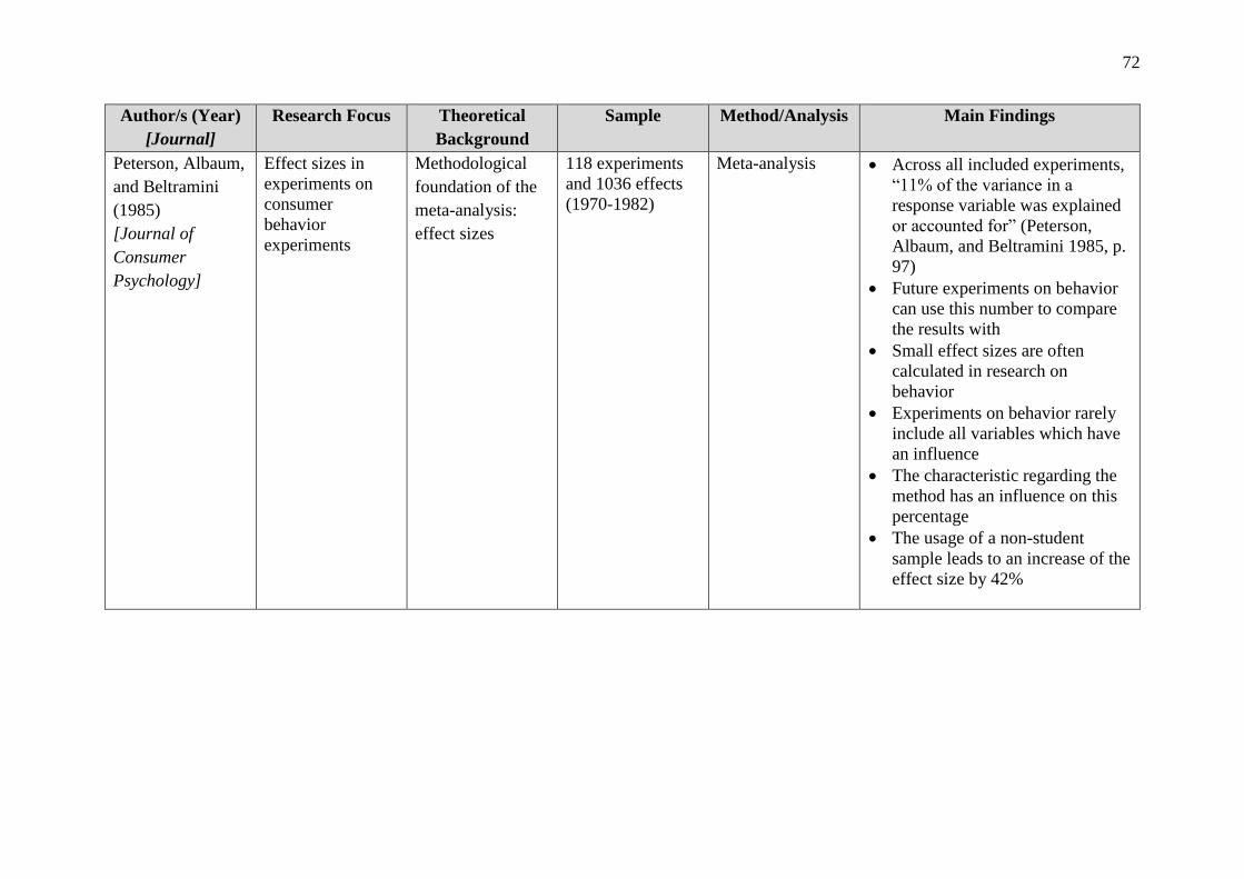
72

Author/s (Year)

[Journal]

Research Focus Theoretical

Background

Sample Method/Analysis Main Findings

Peterson, Albaum,

and Beltramini

(1985)

[Journal of

Consumer

Psychology]

Effect sizes in

experiments on

consumer

behavior

experiments

Methodological

foundation of the

meta-analysis:

effect sizes

118 experiments

and 1036 effects

(1970-1982)

Meta-analysis

• Across all included experiments,

“11% of the variance in a

response variable was explained

or accounted for” (Peterson,

Albaum, and Beltramini 1985, p.

97)

• Future experiments on behavior

can use this number to compare

the results with

• Small effect sizes are often

calculated in research on

behavior

• Experiments on behavior rarely

include all variables which have

an influence

• The characteristic regarding the

method has an influence on this

percentage

• The usage of a non-student

sample leads to an increase of the

effect size by 42%

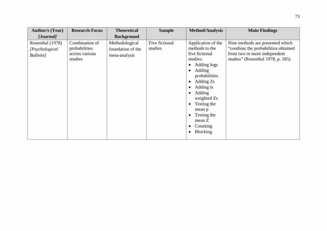
73

Author/s (Year)

[Journal]

Research Focus Theoretical

Background

Sample Method/Analysis Main Findings

Rosenthal (1978)

[Psychological

Bulletin]

Combination of

probabilities

across various

studies

Methodological

foundation of the

meta-analysis

Five fictional

studies

Application of the

methods to the

five fictional

studies:

• Adding logs

• Adding

probabilities

• Adding Zs

• Adding ts

• Adding

weighted Zs

• Testing the

mean p

• Testing the

mean Z

• Counting

• Blocking

Nine methods are presented which

“combine the probabilities obtained

from two or more independent

studies” (Rosenthal 1978, p. 185)

74

Author/s (Year)

[Journal]

Research Focus Theoretical

Background

Sample Method/Analysis Main Findings

Rust, Lehmann,

and Farley (1990)

[Journal of

Marketing

Research]

Estimation of the

publication bias in

meta-analysis

Methodological

foundation of the

meta-analysis

Application of the

method to three

meta-analyses

Derivation of a

maximum

likelihood method

• Publication bias results if studies

with poor outcomes are less

probable to be released in a

journal

• Description of a maximum

likelihood method to estimate

whether a publication bias exists

• The approach further estimates

the share of trials, which are

censored, “the threshold past

which censorship is avoided, and

the probability of censorship if a

potential observation is under the

censorship threshold” (Rust,

Lehmann, and Farley 1990, p.

220)

75

Author/s (Year)

[Journal]

Research Focus Theoretical

Background

Sample Method/Analysis Main Findings

Schmidt and

Hunter (1977)

[Journal of

Applied

Psychology]

• Bayesian

statistical

model

• Validity

generalization

Validity

generalization

- Bayesian approach • Bayesian approach is preferred

over maximum likelihood

methods in order to assess

validation

• The Bayesian model also uses

the outcome of previous studies

to evaluate validity in contrast to

the traditional techniques which

only analyze validity based on

the information of the current

study

• Presentation of a more precise

term for the variance due to the

size of the sample

76

Author/s (Year)

[Journal]

Research Focus Theoretical

Background

Sample Method/Analysis Main Findings

Shocker, Bayus,

and Kim (2004)

[Journal of

Marketing]

Product

complementarity

and substitutes

• Economic

theory

• Intercategory

effects

- Literature review • The demand regarding a product

can be influenced directly or

indirectly by the marketing

activities regarding other

products and by previous

purchase decisions

• Product complementarity means

that the decrease in the price of

the first products results in a

sales growth of a second product

• Substitutes are products if a price

increase of the first product leads

to a sales growth of the second

product

• Intercategory relationships can

be static or dynamic

• Complements can be enhanced if

the introduction of a new product

increases the sales of a current

product in the market by

“improving its functionality”

(Shocker, Bayus, and Kim 2004,

p. 32)

• Complements can augment

existing products by providing a

new advantage which was not

included by the former product

77

Author/s (Year)

[Journal]

Research Focus Theoretical

Background

Sample Method/Analysis Main Findings

Simonson (1989)

[Journal of

Consumer

Research]

• Attraction

effect

• Compromise

effect

• Consumer

behavior in

case of

uncertain

preferences

• Prospect

theory

Attraction

effect

• Compromise

effect

Pilot study:

n = 147 college

students

Study 1:

n = 372 students

Study 2:

n = 100 college

students

Study 3:

n = 23 first-year

graduate students

Pilot study:

t-test

Study 1-3:

• Multinomial

logit analyses

• Multiple

regression

analysis

• Think-aloud

protocols

• If a brand becomes a

compromise option, it is likely to

gain market share

• Both the compromise effect and

the attraction effect are stronger

in a situation in which it is

expected that the choice is to be

justified in front of others

• The choice of the compromise

and the dominating brands are

linked to choices which are more

complex

78

Author/s (Year)

[Journal]

Research Focus Theoretical

Background

Sample Method/Analysis Main Findings

Simonson and

Tversky (1992)

[Journal of

Marketing

Research]

• Context effects

• Tradeoff

contrast

• Attraction

effect

• Compromise

effect

• Extremeness

aversion

• Value

maximization

• Context effects

• Tradeoff

contrast

• Extremeness

aversion

• Sum of

participants

ranges from

100 to 220

• About two

thirds:

undergraduate

and graduate

students of

business

administration

• One third:

undergraduate

and graduate

students of

psychology

22 experiments • Context effects are a robust and

frequent phenomenon

• Asymmetric dominance effect

implies that adding an inferior

alternative to the choice set rises

the share of the superior

alternative

• The compromise effect is

explained by extremeness

aversion

• Adding an extreme alternative

leads to a growth of the share of

the compromise or middle option

in relation to the other extreme

• Polarization means that adding a

middle alternative leads to a

benefit of the alternative of high

quality and price in relation to

the alternative with low price and

quality

79

Author/s (Year)

[Journal]

Research Focus Theoretical

Background

Sample Method/Analysis Main Findings

Tversky and

Simonson (1993)

[Management

Science]

Context-

dependent

preferences

• Classical

theory of

choice

• Value

maximization

• Trade-off

contrast

• Extremeness

aversion

- Development of a

context-dependent

model

• The context-dependent model

describes the tradeoff contrast

and extremeness aversion by two

following elements

• A weighting model includes the

impact of the background context

and a binary comparison model

measures the influence of the

local context

80

Author/s (Year)

[Journal]

Research Focus Theoretical

Background

Sample Method/Analysis Main Findings

Walters (1991)

[Journal of

Marketing]

Influence of retail

price promotions

on product

substitution,

complementary

purchase and

interstore sales

displacement

Product

complementarity

and substitutes

Store level

scanner data and

company records

over 26 weeks

Regression model • Retail price promotions

significantly result in effects for

substitutes and complements

within a store

• The promotion activities in one

store significantly result in a

sales decline regarding

complements and substitutes in

the store of a competitor

81

References

Aguinis, Herman, Dan R. Dalton, Frank A. Bosco, Charles A. Pierce, and Catherine M.

Dalton (2011), “Meta-Analytic Choices and Judgment Calls. Implications for Theory

Building and Testing, Obtained Effect Sizes, and Scholarly Impact,” Journal of

Management, 37 (1), 5–38.

Barendregt, Jan J. and Suhail A. Doi (n.d.), “MetaXL User Guide,” (accessed September 10,

2017), [available at https://www.epigear.com/index_files/metaxl.html].

Borenstein, Michael, Larry V. Hedges, Julian P. T. Higgins, and Hannah R. Rothstein (2010),

Introduction to Meta-Analysis, Reprinted. Chichester: Wiley.

Bühl, Achim (2016), SPSS 23. Einführung in die Moderne Datenanalyse. Myilibrary, 15th ed.

Hallbergmoos: Pearson; Pearson Deutschland GmbH.

Churchill Jr., Gilbert A. and J. P. Peter (1984), “Research Design Effects on the Reliability of

Rating Scales. A Meta-Analysis,” Journal of Marketing Research, 360–75.

Cochran, William G. (1954), “The Combination of Estimates from Different Experiments,”

Biometrics, 10 (1), 101–29.

Cohen, Jacob (1977), Statistical Power Analysis for the Behavioral Sciences. New York:

Acad. Pr.

Cooper, Harris M. (2010), Research Synthesis and Meta-Analysis. A Step-by-Step Approach.

Applied Social Research Methods Series, Vol. 2, 4th ed. Los Angeles: SAGE.

DerSimonian, Rebecca and Nan Laird (1986), “Meta-Analysis in Clinical Trials,” Controlled

Clinical Trials, 7 (3), 177–88.

Dhar, Ravi and Itamar Simonson (2003), “The Effect of Forced Choice on Choice,” Journal

of Marketing Research, 40 (2), 146–60.

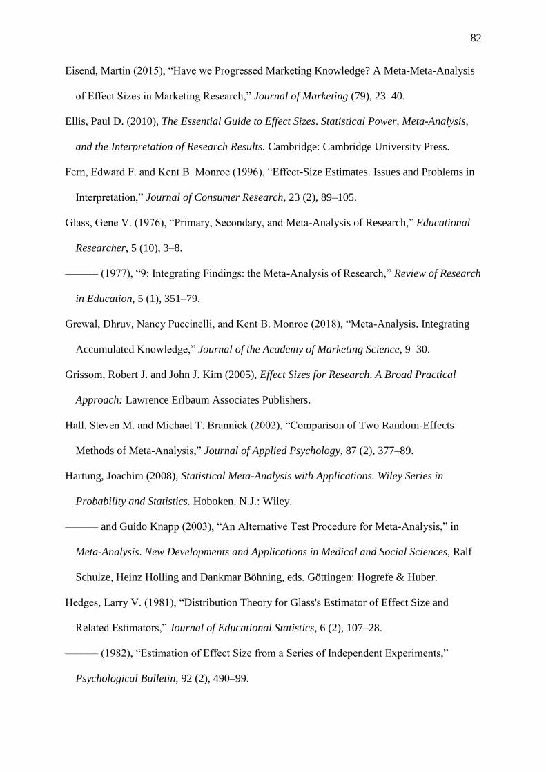
82

Eisend, Martin (2015), “Have we Progressed Marketing Knowledge? A Meta-Meta-Analysis

of Effect Sizes in Marketing Research,” Journal of Marketing (79), 23–40.

Ellis, Paul D. (2010), The Essential Guide to Effect Sizes. Statistical Power, Meta-Analysis,

and the Interpretation of Research Results. Cambridge: Cambridge University Press.

Fern, Edward F. and Kent B. Monroe (1996), “Effect-Size Estimates. Issues and Problems in

Interpretation,” Journal of Consumer Research, 23 (2), 89–105.

Glass, Gene V. (1976), “Primary, Secondary, and Meta-Analysis of Research,” Educational

Researcher, 5 (10), 3–8.

——— (1977), “9: Integrating Findings: the Meta-Analysis of Research,” Review of Research

in Education, 5 (1), 351–79.

Grewal, Dhruv, Nancy Puccinelli, and Kent B. Monroe (2018), “Meta-Analysis. Integrating

Accumulated Knowledge,” Journal of the Academy of Marketing Science, 9–30.

Grissom, Robert J. and John J. Kim (2005), Effect Sizes for Research. A Broad Practical

Approach: Lawrence Erlbaum Associates Publishers.

Hall, Steven M. and Michael T. Brannick (2002), “Comparison of Two Random-Effects

Methods of Meta-Analysis,” Journal of Applied Psychology, 87 (2), 377–89.

Hartung, Joachim (2008), Statistical Meta-Analysis with Applications. Wiley Series in

Probability and Statistics. Hoboken, N.J.: Wiley.

——— and Guido Knapp (2003), “An Alternative Test Procedure for Meta-Analysis,” in

Meta-Analysis. New Developments and Applications in Medical and Social Sciences, Ralf

Schulze, Heinz Holling and Dankmar Böhning, eds. Göttingen: Hogrefe & Huber.

Hedges, Larry V. (1981), “Distribution Theory for Glass's Estimator of Effect Size and

Related Estimators,” Journal of Educational Statistics, 6 (2), 107–28.

——— (1982), “Estimation of Effect Size from a Series of Independent Experiments,”

Psychological Bulletin, 92 (2), 490–99.

83

——— (1983), “A Random Effects Model for Effect Sizes,” Psychological Bulletin, 93 (2),

388–95.

——— and Ingram Olkin (1980), “Vote-Counting Methods in Research Synthesis,”

Psychological Bulletin, 88 (2), 359–69.

——— and ——— (1985), Statistical Methods for Meta-Analysis. Orlando: Acad. Pr.

——— and Jack L. Vevea (1998), “Fixed-and Random-Effects Models in Meta-Analysis,”

Psychological Methods, 3 (4), 486–504.

Higgins, Julian and Simon G. Thompson (2002), “Quantifying Heterogeneity in a Meta-

Analysis,” Statistics in Medicine, 21 (11), 1539–58.

Higgins, Julian P. T., Simon G. Thompson, Jonathan J. Deeks, and Douglas G. Altman

(2003), “Measuring Inconsistency in Meta-Analyses,” British Medical Journal, 327, 557–

60.

Johnson, Blair T., Brian Mullen, and Eduardo Salas (1995), “Comparison of Three Major

Meta-Analytic Approaches,” Journal of Applied Psychology, 80 (1), 94–106.

Kivetz, Ran, Oded Netzer, and V. Srinivasan (2004), “Alternative Models for Capturing the

Compromise Effect,” Journal of Marketing Research, 41 (3), 237–57.

Koschate, Nicole (2008), “Grundlagen Experimenteller Marktforschung,” in Handbuch

Marktforschung. Methoden - Anwendungen - Praxisbeispiele, Andreas Herrmann, Christian

Homburg and Martin Klarmann, eds., 3rd ed. Wiesbaden: Gabler.

Lichters, Marcel, Claudia Brunnlieb, Gideon Nave, Marko Sarstedt, and Bodo Vogt (2016),

“The Influence of Serotonin Deficiency on Choice Deferral and the Compromise Effect,”

Journal of Marketing Research, 53 (2), 183–98.

Lipsey, Mark W. and David B. Wilson (2001), Practical Meta-Analysis: Sage Publications

Thousand Oaks, CA.

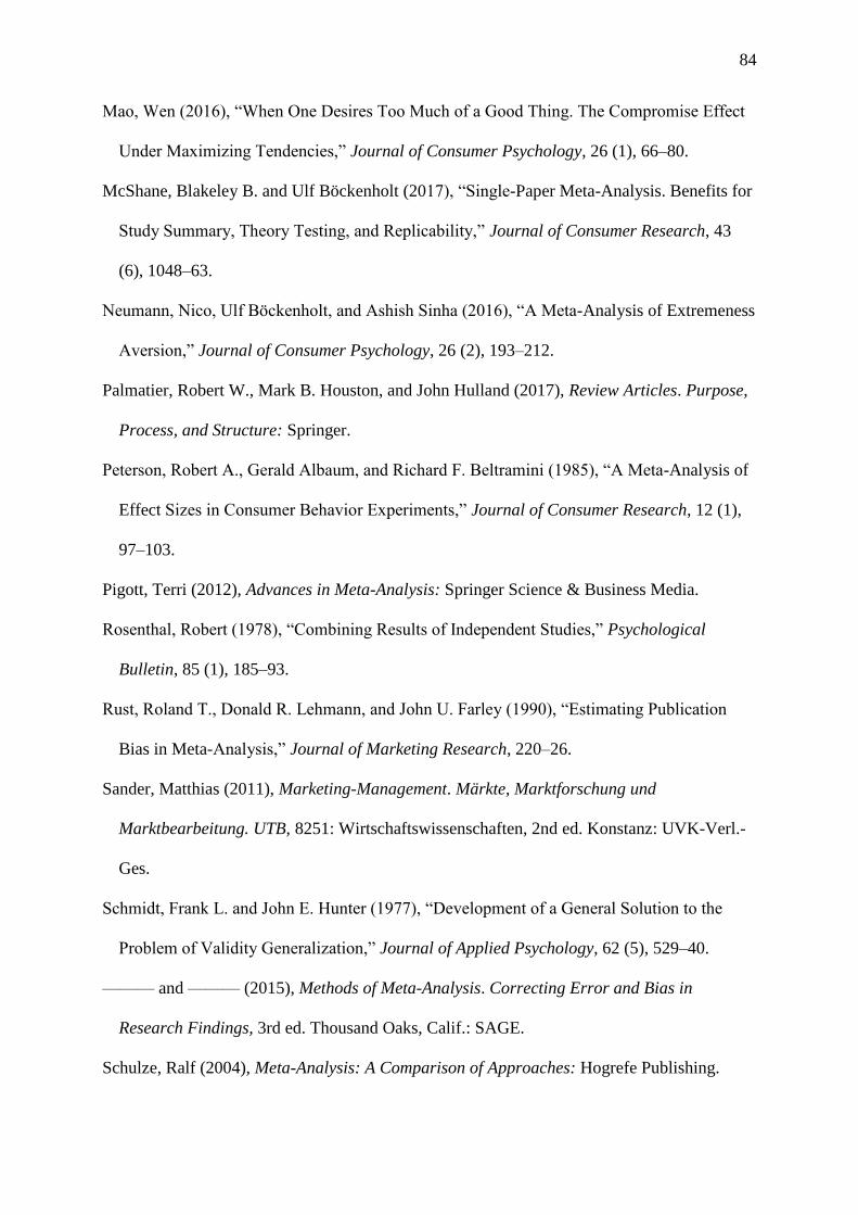
84

Mao, Wen (2016), “When One Desires Too Much of a Good Thing. The Compromise Effect

Under Maximizing Tendencies,” Journal of Consumer Psychology, 26 (1), 66–80.

McShane, Blakeley B. and Ulf Böckenholt (2017), “Single-Paper Meta-Analysis. Benefits for

Study Summary, Theory Testing, and Replicability,” Journal of Consumer Research, 43

(6), 1048–63.

Neumann, Nico, Ulf Böckenholt, and Ashish Sinha (2016), “A Meta-Analysis of Extremeness

Aversion,” Journal of Consumer Psychology, 26 (2), 193–212.

Palmatier, Robert W., Mark B. Houston, and John Hulland (2017), Review Articles. Purpose,

Process, and Structure: Springer.

Peterson, Robert A., Gerald Albaum, and Richard F. Beltramini (1985), “A Meta-Analysis of

Effect Sizes in Consumer Behavior Experiments,” Journal of Consumer Research, 12 (1),

97–103.

Pigott, Terri (2012), Advances in Meta-Analysis: Springer Science & Business Media.

Rosenthal, Robert (1978), “Combining Results of Independent Studies,” Psychological

Bulletin, 85 (1), 185–93.

Rust, Roland T., Donald R. Lehmann, and John U. Farley (1990), “Estimating Publication

Bias in Meta-Analysis,” Journal of Marketing Research, 220–26.

Sander, Matthias (2011), Marketing-Management. Märkte, Marktforschung und

Marktbearbeitung. UTB, 8251: Wirtschaftswissenschaften, 2nd ed. Konstanz: UVK-Verl.-

Ges.

Schmidt, Frank L. and John E. Hunter (1977), “Development of a General Solution to the

Problem of Validity Generalization,” Journal of Applied Psychology, 62 (5), 529–40.

——— and ——— (2015), Methods of Meta-Analysis. Correcting Error and Bias in

Research Findings, 3rd ed. Thousand Oaks, Calif.: SAGE.

Schulze, Ralf (2004), Meta-Analysis: A Comparison of Approaches: Hogrefe Publishing.

85

———, Heinz Holling, and Dankmar Böhning, eds. (2003), Meta-Analysis. New

Developments and Applications in Medical and Social Sciences. Göttingen: Hogrefe &

Huber.

Shocker, Allan D., Barry L. Bayus, and Namwoon Kim (2004), “Product Complements and

Substitutes in the Real World. The Relevance of “Other Products”” Journal of Marketing,

68 (1), 28–40.

Simonson, Itamar (1989), “Choice Based on Reasons. The Case of Attraction and

Compromise Effects,” Journal of Consumer Research, 16 (2), 158–74.

——— and Amos Tversky (1992), “Choice in Context: Tradeoff Contrast and Extremeness

Aversion,” Journal of Marketing Research, 29 (3), 281–95.

Tversky, Amos and Itamar Simonson (1993), “Context-Dependent Preferences,” Management

Science, 39 (10), 1179–89.

Walters, Rockney G. (1991), “Assessing the Impact of Retail Price Promotions on Product

Substitution, Complementary Purchase, and Interstore Sales Displacement,” Journal of

Marketing, 55 (2), 17–28.

Wilcox, Rand R. (2010), Fundamentals of Modern Statistical Methods: Substantially

Improving Power and Accuracy, Second. New York, NY: Springer New York.