kernel visual recognition

7/29/2019 Kernel Visual Recognition

http://slidepdf.com/reader/full/kernel-visual-recognition 1/9

Kernel Descriptors for Visual Recognition

Liefeng BoUniversity of WashingtonSeattle WA 98195, USA

Xiaofeng RenIntel Labs Seattle

Seattle WA 98105, USA

Dieter FoxUniversity of Washington & Intel Labs Seattle

Seattle WA 98195 & 98105, USA

Abstract

The design of low-level image features is critical for computer vision algorithms.Orientation histograms, such as those in SIFT [16] and HOG [3], are the mostsuccessful and popular features for visual object and scene recognition. We high-light the kernel view of orientation histograms, and show that they are equivalentto a certain type of match kernels over image patches. This novel view allowsus to design a family of kernel descriptors which provide a unified and princi-pled framework to turn pixel attributes (gradient, color, local binary pattern, etc.)into compact patch-level features. In particular, we introduce three types of matchkernels to measure similarities between image patches, and construct compactlow-dimensional kernel descriptors from these match kernels using kernel princi-pal component analysis (KPCA) [23]. Kernel descriptors are easy to design andcan turn any type of pixel attribute into patch-level features. They outperform

carefully tuned and sophisticated features including SIFT and deep belief net-works. We report superior performance on standard image classification bench-marks: Scene-15, Caltech-101, CIFAR10 and CIFAR10-ImageNet.

1 Introduction

Image representation (features) is arguably the most fundamental task in computer vision. Theproblem is highly challenging because images exhibit high variations, are highly structured, andlie in high dimensional spaces. In the past ten years, a large number of low-level features overimages have been proposed. In particular, orientation histograms such as SIFT [16] and HOG [3]are the most popular low-level features, essential to many computer vision tasks such as objectrecognition and 3D reconstruction. The success of SIFT and HOG naturally raises questions on how

they measure the similarity between image patches, how we should understand the design choices inthem, and whether we can find a principled way to design and learn comparable or superior low-levelimage features.

In this work, we highlight the kernel view of orientation histograms and provide a unified way tolow-level image feature design and learning. Our low-level image feature extractors, kernel descrip-tors, consist of three steps: (1) design match kernels using pixel attributes; (2) learn compact basisvectors using kernel principle component analysis; (3) construct kernel descriptors by projecting theinfinite-dimensional feature vectors to the learned basis vectors. We show how our framework isapplied to gradient, color, and shape pixel attributes, leading to three effective kernel descriptors.We validate our approach on four standard image category recognition benchmarks, and show thatour kernel descriptors surpass both manually designed and well tuned low-level features (SIFT) [16]and sophisticated feature learning approaches (convolutional networks, deep belief networks, sparsecoding, etc.) [10, 26, 14, 24].

1



The most relevant work to this paper is that of efficient match kernels (EMK) [1], which providesa kernel view to the frequently used Bag-of-Words representation and forms image-level featuresby learning compact low dimensional projections or using random Fourier transformations. Whilethe work on efficient match kernels is interesting, the hand-crafted SIFT features are still used asthe basic building block. Another related work is based on mathematics of the neural response,

which shows that the hierarchical architectures motivated by the neuroscience of the visual cortex isassociated to the derived kernel [24]. Instead, the goal of this paper is to provide a deep understand-ing of how orientation histograms (SIFT and HOG) work, and we can generalize them and designnovel low-level image features based on the kernel insight. Our kernel descriptors are general andprovide a principled way to convert pixel attributes to patch-level features. To the best of our knowl-edge, this is the first time that low-level image features are designed and learned from scratch usingkernel methods; they can serve as the foundation of many computer vision tasks including objectrecognition.

This paper is organized as follows. Section 2 introduces the kernel view of histograms. Our novelkernel descriptors are presented in Section 3, followed by an extensive experimental evaluation inSection 4. We conclude in Section 5.

2 Kernel View of Orientation Histograms

Orientation histograms, such as SIFT [16] and HOG [3], are the most commonly used low-levelfeatures for object detection and recognition. Here we describe the kernel view of such orientationhistograms features, and show how this kernel view can help overcome issues such as orientationbinning. Let θ(z) and m(z) be the orientation and magnitude of the image gradient at a pixel z. InHOG and SIFT, the gradient orientation of each pixel is discretized into a d−dimensional indicatorvector δ (z) = [δ 1(z), · · · , δ d(z)] with

δ i(z) =

1, dθ(z)

2π = i − 1

0, otherwise(1)

where x takes the largest integer less than or equal to x (we will describe soft binning furtherbelow). The feature vector of each pixel z is a weighted indicator vector F (z) = m(z)δ (z). Ag-gregating feature vectors of pixels over an image patch P , we obtain the histogram of oriented

gradients:F h(P ) =

z∈P

m(z)δ (z) (2)

where m(z) = m(z)/

z∈P m(z)2 + g is the normalized gradient magnitude, with g a smallconstant. P is typically a 4 × 4 rectangle in SIFT and an 8 × 8 rectangle in HOG. Without loss of generality, we consider L2-based normalization here. In object detection [3, 5] and matching basedobject recognition [18], linear support vector machines or the L2 distance are commonly applied tosets of image patch features. This is equivalent to measuring the similarity of image patches using alinear kernel in the feature map F h(P ) in kernel space:

K h(P, Q) = F h(P )F h(Q) =z∈P

z∈Q

m(z)m(z)δ (z)δ (z) (3)

where P and Q are patches usually from two different images. In Eq. 3, both k m(z, z) =m(z)m(z) and kδ(z, z) = δ (z)δ (z) are the inner product of two vectors and thus are positivedefinite kernels. Therefore, K h(P, Q) is a match kernel over sets (here the sets are image patches)as in [8, 1, 11, 17, 7]. Thus Eq. 3 provides a kernel view of HOG features over image patches. Forsimplicity, we only use one image patch here; it is straightforward to extend to sets of image patches.

The hard binning underlying Eq. 1 is only for ease of presentation. To get a kernel view of softbinning [13], we only need to replace the delta function in Eq. 1 by the following, soft δ (·) function:

δ i(z) = max(cos(θ(z) − ai)9, 0) (4)

where a(i) is the center of the i−th bin. In addition, one can easily include soft spatial binning bynormalizing gradient magnitudes using the corresponding spatial weights. The L2 distance betweenP and Q can be expressed as D(P, Q) = 2− 2F (P )F (Q) as we know F (P )F (P ) = 1, and thekernel view can be provided in the same manner.

2



Figure 1: Pixel attributes. Left : Gradient orientation representation. To measure similarity betweentwo pixel orientation gradients θ and θ, we use the L2 norm between the normalized gradient vectorsθ = [sin(θ) cos(θ)] and θ = [sin(θ) cos(θ)]. The red dots represent the normalized gradientvectors, and the blue line represents the distance between them. Right : Local binary patterns. Thevalues indicate brightness of pixels in a 3×3 patch. Red pixels have intensities larger than the centerpixel, blue pixels are darker. The 8-dimensional indicator vector is the resulting local binary pattern.

Note that the kernel k m(z, z

) measuring the similarity of gradient magnitudes of two pixels is linearin gradient magnitude. kδ(z, z) measures the similarity of gradient orientations of two pixels: 1 if two gradient orientations are in the same bin, and 0 otherwise (Eq.1, hard binning). As can be seen,this kernel introduces quantization errors and could lead to suboptimal performance in subsequentstages of processing. While soft binning results in a smoother kernel function, it still suffers fromdiscretization. This motivates us to search for alternative match kernels which can measure thesimilarity of image patches more accurately.

3 Kernel Descriptors

3.1 Gradient, Color, and Shape Match Kernels

We introduce the following gradient match kernel, K grad, to capture image variations:

K grad(P, Q) = z∈P

z∈Q

m(z)m(z)ko(θ(z), θ(z))k p(z, z) (5)

where k p(z, z) = exp(−γ pz−z2) is a Gaussian position kernel with z denoting the 2D position

of a pixel in an image patch (normalized to [0, 1]), and ko(θ(z), θ(z)) = exp(−γ oθ(z)− θ(z)2)is a Gaussian kernel over orientations. To estimate the difference between orientations at pixels zand z, we use the following normalized gradient vectors in the kernel function ko:θ(z) = [sin(θ(z)) cos(θ(z))] . (6)

The L2 distance between such vectors measures the difference of gradient orientations very well (seeFigure 1). Note that computing the L2 distance on the raw angle values θ instead of the normalized

gradient vectors

θ would cause wrong similarity in some cases. For example, consider the two angles

2π − 0.01and

0.01, which have very similar orientation but very large

L2distance.

To summarize, our gradient match kernel K grad consists of three kernels: the normalized linearkernel is the same as that in the orientation histograms, weighting the contribution of each pixelusing gradient magnitudes; the orientation kernel ko computes the similarity of gradient orientations;and the position Gaussian kernel k p measures how close two pixels are spatially.

The kernel view of orientation histograms provides a simple, unified way to turn pixel attributes intopatch-level features. One immediate extension is to construct color match kernels over pixel values:

K col(P, Q) =z∈P

z∈Q

kc(c(z), c(z))k p(z, z) (7)

where c(z) is the pixel color at position z (intensity for gray images and RGB values for color

images). kc(c(z), c(z)) = exp

−γ cc(z) − c(z)2

measures how similar two pixel values are.

3



While the gradient match kernel can capture image variations and the color match kernel can de-scribe image appearance, we find that a match kernel over local binary patterns can capture localshape more effectively: [19]:

K shape(P, Q) =

z∈P z∈Q s(z)

s(z)kb(b(z), b(z))k p(z, z) (8)

where s(z) = s(z)/

z∈P s(z)2 + s, s(z) is the standard deviation of pixel values in the

3 × 3 neighborhood around z, s a small constant, and b(z) is binary column vector binarizesthe pixel value differences in a local window around z (see Fig. 1(right )). The normalized lin-ear kernel s(z)s(z) weighs the contribution of each local binary pattern, and the Gaussian kernelkb(b(z), b(z)) = exp(−γ bb(z)−b(z)2) measures shape similarity through local binary patterns.

Match kernels defined over various pixel attributes provide a unified way to generate a rich, diversevisual feature set, which has been shown to be very successful to boost recognition accuracy [6]. Asvalidated by our own experiments, gradient, color and shape match kernels are strong in their ownright and complement one another. Their combination turn out to be always (much) better than thebest individual feature.

3.2 Learning Compact Features

Match kernels provide a principled way to measure the similarity of image patches, but evaluatingkernels can be computationally expensive when image patches are large [1]. Both for computationalefficiency and for representational convenience, we present an approach to extract the compact low-dimensional features from match kernels: (1) uniformly and densely sample sufficient basis vectorsfrom support region to guarantee accurate approximation to match kernels; (2) learn compact basisvectors using kernel principal component analysis. An important advantage of our approach is thatno local minima are involved, unlike constrained kernel singular value decomposition [1].

We now describe how our compact low-dimensional features are extracted from the gradient kernelK grad; features for the other kernels can be generated the same way. Rewriting the kernels in Eq. 5

as inner products ko(

θ(z),

θ(z)) = φo(

θ(z))φo(

θ(z)), k p(z, z) = φ p(z)φ p(z), we can derive

the following feature over image patches:

F grad(P ) = z∈P

m(z)φo(θ(z)) ⊗ φ p(z) (9)

where ⊗ is the tensor product. For this feature, it follows that F grad(P )F grad(Q) = K grad(P, Q).Because we use Gaussian kernels, F grad(P ) is an infinite-dimensional vector.

A straightforward way to dimension reduction is to sample sufficient image patches from trainingimages and perform KPCA for match kernels. However, such approach makes the learned featuresdepend on the task at hand. Moreover, KPCA can become computationally infeasible when thenumber of patches is very large.

Sufficient Finite-dimensional Approximation. We present an approach to approximate match ker-nels directly without requiring any image. Following classic methods, we learn finite-dimensionalfeatures by projecting F grad(P ) into a set of basis vectors. A key issue in this projection processis how to choose a set of basis vectors which makes the finite-dimensional kernel approximate well

the original kernel. Since pixel attributes are low-dimensional vectors, we can achieve a very goodapproximation by sampling sufficient basis vectors using a fine grid over the support region. For

example, consider the Gaussian kernel ko(θ(z), θ(z)) over gradient orientation. Given a set of ba-

sis vectors {φo(xi)}doi=1 where xi are sampled normalized gradient vectors, we can approximate a

infinite-dimensional vector φo(θ(z)) by its projection into the space spanned by the set of these dobasis vectors. Following the formulation in [1], such a procedure is equivalent to using a finite-dimensional kernel:ko(θ(z), θ(z)) = ko(θ(z), X )

Ko

−1ij

ko(θ(z), X ) =Gko(θ(z), X )

Gko(θ(z), X )

(10)

where ko(

θ(z), X ) = [ko(

θ(z), x1), · · · , ko(

θ(z), xdo)] is a do × 1 vector,K

ois a do × do matrix

withKoij = ko(xi, xj), andK

o

−1 = GG. The resulting feature map

φo(

θ(z)) = Gko(

θ(z), X )

4



0 2 4 6

0

0.2

0.4

0.6

0.8

1

Ground Truth

10 Grid App

14 Grid App

16 Grid App

0 100 200 300 400 500−1

0

1

2

3

4

5x 10

−4

Dimensionality

R M

S E

Kgrad

Kcol

Kshape

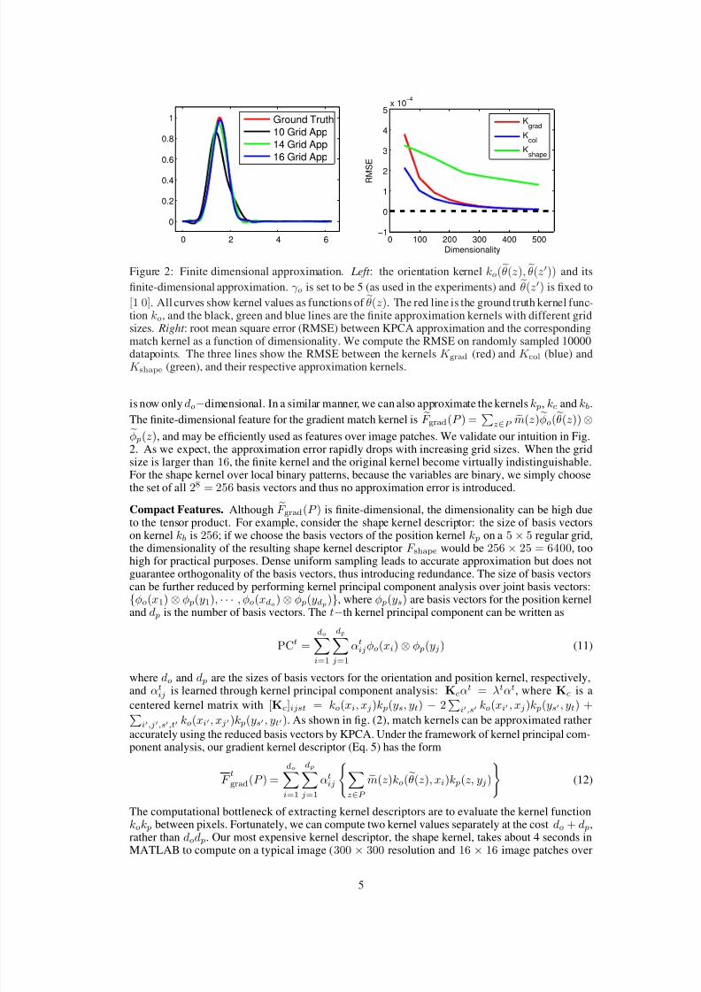
Figure 2: Finite dimensional approximation. Left : the orientation kernel ko(θ(z), θ(z)) and its

finite-dimensional approximation. γ o is set to be 5 (as used in the experiments) and θ(z) is fixed to

[1 0]. All curves show kernel values as functions of θ(z). The red line is the ground truth kernel func-tion ko, and the black, green and blue lines are the finite approximation kernels with different gridsizes. Right : root mean square error (RMSE) between KPCA approximation and the correspondingmatch kernel as a function of dimensionality. We compute the RMSE on randomly sampled 10000datapoints. The three lines show the RMSE between the kernels K grad (red) and K col (blue) andK shape (green), and their respective approximation kernels.

is now only do−dimensional. In a similar manner, we can also approximate the kernels k p, kc and kb.

The finite-dimensional feature for the gradient match kernel is F grad(P ) =

z∈P m(z)φo(θ(z))⊗φ p(z), and may be efficiently used as features over image patches. We validate our intuition in Fig.2. As we expect, the approximation error rapidly drops with increasing grid sizes. When the gridsize is larger than 16, the finite kernel and the original kernel become virtually indistinguishable.For the shape kernel over local binary patterns, because the variables are binary, we simply choosethe set of all 28 = 256 basis vectors and thus no approximation error is introduced.

Compact Features. Although F grad(P ) is finite-dimensional, the dimensionality can be high due

to the tensor product. For example, consider the shape kernel descriptor: the size of basis vectorson kernel kb is 256; if we choose the basis vectors of the position kernel k p on a 5 × 5 regular grid,the dimensionality of the resulting shape kernel descriptor F shape would be 256 × 25 = 6400, toohigh for practical purposes. Dense uniform sampling leads to accurate approximation but does notguarantee orthogonality of the basis vectors, thus introducing redundance. The size of basis vectorscan be further reduced by performing kernel principal component analysis over joint basis vectors:{φo(x1) ⊗ φ p(y1), · · · , φo(xdo) ⊗ φ p(ydp)}, where φ p(ys) are basis vectors for the position kerneland d p is the number of basis vectors. The t−th kernel principal component can be written as

PCt =

doi=1

dpj=1

αtijφo(xi) ⊗ φ p(yj) (11)

where do and d p are the sizes of basis vectors for the orientation and position kernel, respectively,

and αt

ij is learned through kernel principal component analysis:K

cαt

= λt

αt

, whereK

c is acentered kernel matrix with [Kc]ijst = ko(xi, xj)k p(ys, yt) − 2i,s ko(xi , xj)k p(ys , yt) +i,j,s,t ko(xi , xj)k p(ys , yt). As shown in fig. (2), match kernels can be approximated rather

accurately using the reduced basis vectors by KPCA. Under the framework of kernel principal com-ponent analysis, our gradient kernel descriptor (Eq. 5) has the form

F t

grad(P ) =

doi=1

dpj=1

αtij

z∈P

m(z)ko(θ(z), xi)k p(z, yj)

(12)

The computational bottleneck of extracting kernel descriptors are to evaluate the kernel functionkok p between pixels. Fortunately, we can compute two kernel values separately at the cost do + d p,rather than dod p. Our most expensive kernel descriptor, the shape kernel, takes about 4 seconds inMATLAB to compute on a typical image (300 × 300 resolution and 16 × 16 image patches over

5



8×8 grids). It is about 1.5 seconds for the gradient kernel descriptor, compared to about 0.4 secondsfor SIFT under the same setting. A more efficient GPU-based implementation will certainly reducethe computation time for kernel descriptors such that real time applications become feasible.

4 Experiments

We compare gradient (KDES-G), color (KDES-C), and shape (KDES-S) kernel descriptors to SIFTand several other state of the art object recognition algorithms on four publicly available datasets:Scene-15, Caltech101, CIFAR10, and CIFAR10-ImageNet (a subset of ImageNet). For gradient andshape kernel descriptors and SIFT, all images are transformed into grayscale ([0, 1]) and resized to beno larger than 300× 300 pixels with preserved ratio. Image intensity or RGB values are normalizedto [0 1]. We extracted all low level features with 16×16 image patches over dense regular grids withspacing of 8 pixels. We used publicly available dense SIFT code at http://www.cs.unc.edu/ lazeb-nik [13], which includes spatial binning, soft binning and truncation (nonlinear cutoff at 0.2), andhas been demonstrated to obtain high accuracy for object recognition. For our gradient kernel de-scriptors we use the same gradient computation as used for SIFT descriptors. We also evaluate theperformance of the combination of the three kernel descriptors (KDES-A) by simply concatenatingthe image-level features vectors.

Instead of spatial pyramid kernels, we compute image-level features using efficient match kernels(EMK), which has been shown to produce more accurate quantization. We consider 1×1, 2×2 and4 × 4 pyramid sub-regions (see [1]), and perform constrained kernel singular value decomposition(CKSVD) to form image-level features, using 1,000 visual words (basis vectors in CKSVD) learnedby K-means from about 100,000 image patch features. We evaluate classification performance withaccuracy averaged over 10 random training/testing splits with the exception of the CIFAR10 dataset,where we report the accuracy on the test set. We have experimented both with linear SVMs andLaplacian kernel SVMs and found that Laplacian kernel SVMs over efficient match kernel featuresare always better than linear SVMs (see (§4.2)). We use Laplacian kernel SVMs in our experiments(except for the tiny image dataset CIFAR10).

4.1 Hyperparameter Selection

We select kernel parameters using a subset of ImageNet. We retrieve 8 everyday categories fromthe ImageNet collection: apple, banana, box, coffee mug, computer keyboard, laptop, soda can andwater bottle. We choose basis vectors for ko, kc, and k p from 25, 5 × 5 × 5 and 5 × 5 uniformgrids, respectively, which give sufficient approximations to the original kernels (see also Fig. 2).We optimize the dimensionality of KPCA and match kernel parameters jointly using exhaustive gridsearch. Our experiments suggest that the optimal parameter settings are r = 200 (dimensionalityof kernel descriptors), γ o = 5, γ c = 4, γ b = 2, γ p = 3, g = 0.8 and s = 0.2 (fig. 3). In thefollowing experiments, we will keep these values fixed, even though the performance may improveif considering task-dependent hyperparameter selection.

4.2 Benchmark Comparisons

Scene-15. Scene-15 is a popular scene recognition benchmark from [13] which contains 15 scene

categories with 200 to 400 images in each. SIFT features have been extensively used on Scene-15. Following the common experimental setting, we train our models on 1,500 randomly selectedimages (100 images per category) and test on the rest. We report the averaged accuracy of SIFT,KDES-S, KDES-C, KDES-G, and KDES-A over 10 random training/test splits in Table 1. As wesee, both gradient and shape kernel descriptors outperform SIFT with a margin. Gradient kerneldescriptors and shape kernel descriptors have similar performance. It is not surprising that theintensity kernel descriptor has a lower accuracy, as all the images are grayscale. The combination of the three kernel descriptors further boosts the performance by about 2 percent. Another interestingfinding is that Laplacian kernel SVMs are significantly better than linear SVMs, 86.7%.

In our recognition system, the accuracy of SIFT is 82.2% compared to 81.4% in spatial pyramidmatch (SPM). We also tried to replace SIFT features with our gradient and shape kernel descrip-tors in SPM, and both obtained 83.5% accuracy, 2 percent higher than SIFT features. To our bestknowledge, our gradient kernel descriptor alone outperforms the best published result 84.2% [27].

6



100 200 300 4000.7

0.75

0.8

0.85

KDES−S

KDES−G

0 0.2 0.4 0.6 0.8 1

0.74

0.76

0.78

0.8

0.82

KDES−S

KDES−G

0 2 4 6

0.74

0.76

0.78

0.8

0.82

KDES−S

KDES−G

Figure 3: Hyperparameter selection. left : Accuracy as functions of feature dimensionality for orien-tation kernel (KDES-G) and shape kernel (KDES-S), respectively. center : Accuracy as functions of g and s. right : Accuracy as function of γ o and γ b.

Methods SIFT KDES-C KDES-G KDES-S KDES-ALinear SVM 76.7±0.7 38.5±0.4 81.6±0.6 79.8±0.5 81.9±0.6

Laplacian kernel SVM 82.2±0.9 47.9±0.8 85.0±0.6 84.9±0.7 86.7±0.4

Table 1: Comparisons of recognition accuracy on Scene-15: kernel descriptors and their combination vs SIFT.

Caltech-101. Caltech-101 [15] consists of 9,144 images in 101 object categories and one back-ground category. The number of images per category varies from 31 to 800. Because many re-searchers have reported their results on Caltech-101, we can directly compare our algorithm to theexisting ones. Following the standard experimental setting, we train classifiers on 30 images and teston no more than 50 images per category. We report our results in Table 2. We compare our kerneldescriptors with recently published results obtained both by low-level feature learning algorithms,convolutional deep belief networks (CDBN), and sparse coding methods: invariant predictive sparsedecomposition (IPSD) and locality-constrained linear coding. We observe that SIFT features in con-

junction with efficient match kernels work well on this dataset and obtain 70.8% accuracy using asingle patch size, which beat SPM with the same SIFT features by a large margin. Both our gradientkernel descriptor and shape kernel descriptor are superior to CDBN by a large margin.

We have performed feature extraction with three different patch sizes: 16×16, 25× 25 and 31× 31and reached the same conclusions with many other researchers: multiple patch sizes (scales) canboost the performance by a few percent compared to the single patch size. Notice that both naiveBayesian nearest neighbor (NBNN) and locality-constrained linear coding should be compared toour kernel descriptors over multiple patch sizes because both of them used multiple scales to boostthe performance. Using only our gradient kernel descriptor obtains 75.2% accuracy, higher than theresults obtained by all other single feature based methods, to our best knowledge. Another findingis that the combination of three kernel descriptors outperforms any single kernel descriptor. Wenote that better performance has been reported with the use of more image features [6]. Our goalin this paper is to evaluate the strengths of kernel descriptors. To improve accuracy further, kerneldescriptors can be combined with other types of image features.

CIFAR-10. CIFAR-10 is a labeled subset of the 80 million tiny images dataset [25, 12]. Thisdataset consists of 60,000 32x32 color images in 10 categories, with 5,000 images per category as

training set and 1,000 images per category as test set. Deep belief networks have been extensivelyinvestigated on this dataset [21, 22]. We extract kernel descriptors over 8×8 image patches per pixel.Efficient match kernels over the three spatial grids 1×1, 2×2, and 3×3 are used to generate image-level features. The resulting feature vectors have a length of (1+4+9)∗1000(visual words)= 14000per kernel descriptor. Linear SVMs are trained due to the large number of training images.

SPM [13] 64.4±0.5 kCNN [28] 67.4 KDES-C 40.8±0.9 KDES-C(M) 42.4±0.5

NBNN [2] 73.0 IPSD [10] 56.0 KDES-G 73.3±0.6 KDES-G(M) 75.2±0.4

CDBN [14] 65.5 LLC [26] 73.4 ±0.5 KDES-S 68.2±0.7 KDES-S(M) 70.3±0.6

SIFT 70.8±0.8 SIFT(M) 73.2±0.5 KDES-A 74.5±0.8 KDES-A(M) 76.4±0.7

Table 2: Comparisons on Caltech-101. Kernel descriptors are compared to recently published re-sults. (M) indicates that features are extracted with multiple image patch sizes.

7



LR 36.0 GRBM, ZCAd images 59.6 mRBM 59.7 KDES-C 53.9SVM 39.5 GRBM 63.8 cRBM 64.7 KDES-G 66.3

GIST[20] 54.7 fine-tuning GRBM 64.8 mcRBM 68.3 KDES-S 68.2SIFT 65.6 GRBM two layers 56.6 mcRBM-DBN 71.0 KDES-A 76.0

Table 3: Comparisons on CIFAR-10. Both logistic regression and SVMs are trained over imagepixels.

Methods SIFT KDES-C KDES-G KDES-S KDES-ALaplacian kernel SVMs 66.5 ±0.4 56.4±0.8 69.0 ±0.8 70.5±0.7 75.2±0.7

Table 4: Comparisons on CIFAR10-ImageNet, subset of ImageNet using the 10 CIFAR categories.

We compare our kernel descriptors to deep networks [14, 9] and several baselines in table 3. Oneimmediate observation is that sophisticated feature extractions are significantly better than raw pixelfeatures. Linear logistic regression and linear SVMs over raw pixels only have accuracies of 36%and 39.5%, respectively, over 30 percent lower than deep belief networks and our kernel descriptors.

SIFT features still work well on tiny images and have an accuracy of 65.2%. Color kernel descriptor,KDES-C, has 53.9% accuracy. This result is a bit surprising since each category has a large colorvariation. A possible explanation is that spatial information can help a lot. To validate our intu-itions, we also evaluated the color kernel descriptor without spatial information (kernel features areextracted on 1 × 1 spatial grid), and only obtained 38.5% accuracy, 18 percent lower than the colorkernel descriptor over pyramid spatial grids. KDES-G is slightly better than SIFT features. Theshape kernel feature, KDES-S, has accuracy of 68.2%, and is the best single feature on this dataset.Combing the three kernel descriptors, we obtain the best performance of 76%, 5 percent higher thanthe most sophisticated deep network mcRBM-DBN, which model pixel mean and covariance jointlyusing factorized third-order Boltzmann machines.

CIFAR-10-ImageNet. Motivated by CIFAR-10, we collect a labeled subset of ImageNet [4] byretrieving 10 categories used in ImageNet: Airplane, Automobile, Bird, Cat, Deer, Dog, Frog, Horse,Ship and Truck. The total number of images is 15,561 with more than 1,200 images per category.This dataset is very challenging due to the following facts: multiple objects can appear in one image,only a small part of objects are visible, backgrounds are cluttered, and so on. We train models on1,000 images per class and test on 200 images per category. We report the averaged results over 10random training/test splits in Table 4. We can’t finish running deep belief networks in a reasonabletime since they are slow for running images of this scale. Both gradient and shape kernel descriptorsachieve higher accuracy than SIFT features, which again confirms that our gradient kernel descriptorand shape kernel descriptor outperform SIFT features on high resolution images with the samecategory as CIFAR-10. We also ran the experiments on the downsized images, no larger than 50×50with preserved ratio. We observe that the accuracy drops 4-6 percents compared to those on highresolution images. This validates that high resolution is helpful for object recognition.

5 Conclusion

We have proposed a general framework, kernel descriptors, to extract low-level features from imagepatches. Our approach is able to turn any pixel attribute into patch-level features in a unified andprincipled way. Kernel descriptors are based on the insight that the inner product of orientation his-tograms is a particular match kernel over image patches. We have performed extensive comparisonsand confirmed that kernel descriptors outperform both SIFT features and hierarchical feature learn-ing, where the former is the default choice for object recognition and the latter is the most popularlow-level feature learning technique. To our best knowledge, we are the first to show how kernelmethods can be applied for extracting low-level image features and show superior performance. Thisopens up many possibilities for learning low-level features with other kernel methods. Consideringthe huge success of kernel methods in the last twenty years, we believe that this direction is worthbeing pursued. In the future, we plan to investigate alternative kernels for low-level feature learningand learn pixel attributes from large image data collections such as ImageNet.

8



References

[1] L. Bo and C. Sminchisescu. Efficient Match Kernel between Sets of Features for Visual Recog-nition. In NIPS , 2009.

[2] O. Boiman, E. Shechtman, and M. Irani. In defense of nearest-neighbor based image classifi-

cation. In CVPR, 2008.[3] N. Dalal and B. Triggs. Histograms of oriented gradients for human detection. In CVPR, 2005.

[4] J. Deng, W. Dong, R. Socher, L. Li, K. Li, and L. Fei-fei. ImageNet: A Large-Scale Hierar-chical Image Database. In CVPR, 2009.

[5] P. Felzenszwalb, D. McAllester, and D. Ramanan. A discriminatively trained, multiscale,deformable part model. In CVPR, 2008.

[6] P. Gehler and S. Nowozin. On feature combination for multiclass object classification. In ICCV , 2009.

[7] K. Grauman and T. Darrell. The pyramid match kernel: discriminative classification with setsof image features. In ICCV , 2005.

[8] D. Haussler. Convolution kernels on discrete structures. Technical report, 1999.

[9] K. Jarrett, K. Kavukcuoglu, M. Ranzato, and Y. LeCun. What is the best multi-stage architec-

ture for object recognition? In ICCV , 2009.[10] K. Kavukcuoglu, M. Ranzato, R. Fergus, and Y. LeCun. Learning invariant features through

topographic filter maps. In CVPR, 2009.

[11] R. Kondor and T. Jebara. A kernel between sets of vectors. In ICML, 2003.

[12] A. Krizhevsky. Learning multiple layers of features from tiny images. Technical report, 2009.

[13] S. Lazebnik, C. Schmid, and J. Ponce. Beyond bags of features: Spatial pyramid matching forrecognizing natural scene categories. In CVPR, 2006.

[14] H. Lee, R. Grosse, R. Ranganath, and A. Ng. Convolutional deep belief networks for scalableunsupervised learning of hierarchical representations. In ICML, 2009.

[15] F. Li, R. Fergus, and P. Perona. One-shot learning of object categories. IEEE PAMI , 2006.

[16] D. Lowe. Distinctive image features from scale-invariant keypoints. IJCV , 60:91–110, 2004.

[17] S. Lyu. Mercer kernels for object recognition with local features. In CVPR, 2005.[18] K. Mikolajczyk and C. Schmid. A performance evaluation of local descriptors. IEEE PAMI ,

27(10):1615–1630, 2005.

[19] T. Ojala, M. Pietik ainen, and T. Maenpaa. Multiresolution gray-scale and rotation invarianttexture classification with local binary patterns. IEEE PAMI , 24(7):971–987, 2002.

[20] A. Oliva and A. Torralba. Modeling the shape of the scene: A holistic representation of thespatial envelope. IJCV , 42(3):145–175, 2001.

[21] M. Ranzato, Krizhevsky A., and G. Hinton. Factored 3-way restricted boltzmann machines formodeling natural images. In AISTATS , 2010.

[22] M. Ranzato and G. Hinton. Modeling pixel means and covariances using factorized third-orderboltzmann machines. In CVPR, 2010.

[23] B. Scholkopf, A. Smola, and K. Muller. Nonlinear component analysis as a kernel eigenvalue

problem. Neural Computation, 10:1299–1319, 1998.

[24] S. Smale, L. Rosasco, J. Bouvrie, A. Caponnetto, and T. Poggio. Mathematics of the neuralresponse. Foundations of Computational Mathematics, 10(1):67–91, 2010.

[25] A. Torralba, R. Fergus, and W. Freeman. 80 million tiny images: A large data set for nonpara-metric object and scene recognition. IEEE PAMI , 30(11):1958–1970, 2008.

[26] J. Wang, J. Yang, K. Yu, F. Lv, T. Huang, and Y. Guo. Locality-constrained linear coding forimage classification. In CVPR, 2010.

[27] J. Wu and J. Rehg. Beyond the euclidean distance: Creating effective visual codebooks usingthe histogram intersection kernel. 2002.

[28] K. Yu, W. Xu, and Y. Gong. Deep learning with kernel regularization for visual recognition.In NIPS , 2008.

9

kernel visual recognition

Documents