(kernel) density estimation · create a phase space from the building blocks provided. optionally...

(Kernel) Density EstimationIML WG meeting: Unsupervised learning

Anton Poluektov

University of Warwick, UKBudker Institute of Nuclear Physics, Novosibirsk, Russia

25 August 2016

Anton Poluektov (Kernel) Density Estimation IML WG meeting, 25/08/2016 1/27

Introduction

No need to explain that the essential part of every HEP analysis isdensity estimation.

Modelled PDF when we need to measure some parameters from ML fitEmpirical PDF (e.g. KeysPDF, polynomial) when we need some ad hocdescription of some shape (background, efficiency, ...)

Speaking in terms of today’s meeting, density estimation is anexample of unsupervised learning

Take a (training) sampleTry to predict response (probability density) for a point that is not inthe sample.

Here I will concentrate on model-independent density estimation,mostly kernel density estimation (KDE), based on experience fromLHCb analyses.


Simplest case: histogramming

Simplest method of density estimation: histogramming. Certainly, no needto tell you about it.Frequently used extension of this technique at LHCb: cubic splinesmoothing (1D, 2D). See, e.g., [PRD 90, 072003 (2014)]

'm0 0.2 0.4 0.6 0.8 1

'θ

00.10.20.30.40.50.60.70.80.9

1

Eff

icie

ncy

0

0.0005

0.001

0.0015

0.002

0.0025

0.003

0.0035

0.004

(a)LHCb Simulation

Efficiency over 2D phase space ofBs → DKπ decay.

Interpolation by cubic splinebetween bins.

Continuous PDF (and its 1stand 2nd derivatives).

Binning effect is still present.


http://arxiv.org/abs/1407.7712

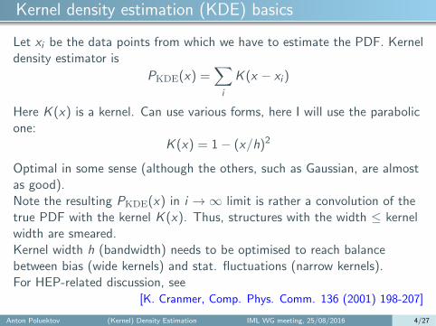
Kernel density estimation (KDE) basics

Let xi be the data points from which we have to estimate the PDF. Kerneldensity estimator is

PKDE(x) =∑i

K (x − xi )

Here K (x) is a kernel. Can use various forms, here I will use the parabolicone:

K (x) = 1− (x/h)2

Optimal in some sense (although the others, such as Gaussian, are almostas good).Note the resulting PKDE(x) in i →∞ limit is rather a convolution of thetrue PDF with the kernel K (x). Thus, structures with the width ≤ kernelwidth are smeared.Kernel width h (bandwidth) needs to be optimised to reach balancebetween bias (wide kernels) and stat. fluctuations (narrow kernels).For HEP-related discussion, see

[K. Cranmer, Comp. Phys. Comm. 136 (2001) 198-207]


http://arxiv.org/abs/hep-ex/0011057

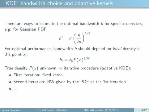
KDE: bandwidth choice and adaptive kernels

There are ways to estimate the optimal bandwidth h for specific densities,e.g. for Gaussian PDF

h∗ = σ

(4

3n

)1/5

For optimal performance, bandwidth h should depend on local density inthe point xi :

hi = h0P(xi )1/N

True density P(x) unknown ⇒ iterative procedure (adaptive KDE):

First iteration: fixed kernel

Second iteration: BW given by the PDF at the 1st iteration.

...


KDE implementations

RooFit: RooKeysPDF (1-dim), RooNDKeysPDF (N-dim).

Gaussian kernelBoth fixed and adaptive kernelsBoundary correction using data reflection

scikit-learn: sklearn.neighbors.KernelDensity.

Choice of various kernelsOnly fixed kernelDifferent metricsOptimisation using KD-tree ⇒ faster lookup

My own implementation (Meerkat): see below

Attempt to solve problems related to boundary effects and curse ofdimensionality.


KDE: boundary effects

Ptrue(x) = 1+3x2+10e−x2/0.12

The usual problem with KDE is boundaryeffects.Methods to correct for this:

Data reflection.

Kernel modification near boundary.

Normally work with simple boundaries (1D,linear). Not easy to apply to e.g. conven-tional Dalitz plots.


KDE: correcting for boundary effect

Ptrue(x) = 1+3x2+10e−x2/0.12

Simple correction: divide result of KDE bythe convolution of kernel with flat density:

Pcorr(x) =

N∑i=1

K(x−xi )

(U⊗K)(x) for x ∈ X ,

0 otherwise.

U(x) =

{1 for x ∈ X ,0 otherwise.


KDE: correcting for boundary effect

Ptrue(x) = 1+3x2+10e−x2/0.12

Pappr = 1 + 10e−x2/0.12

Suppose we approximately know how thePDF behaves at the boundaries. A moresophisticated correction:

Pcorr(x) =

N∑i=1

K (x − xi )

(Pappr ⊗ K )(x)× Pappr(x).

replaces KDE by an approximation PDFat boundaries and in regions with narrowstructures.


Relative KDE

Pcorr(x) =

N∑i=1

K (x − xi )

(Pappr ⊗ K )(x)× Pappr(x).

In other words, we represent the PDF as a product:

Pcorr(x) = f (x)Pappr(x)

where Pappr(x) is known and describes narrow structures and boundaries,and f (x) is slowly-varying and is represented by the kernel density.

An intermediate solution between the model-based and model-independentdensity estimators.

Can be generalised to any complex boundaries, weighted distributions(including negative weights, sWeights), variable (adaptive) kernels.

[A.P., JINST 10 P02011 (2015)]



Relative KDE: multidimensional case

So, we have an approach that performs KDE over some approximationPDF. How does this help in the case of multiple dimensions?Multiple dimensions typically need wide kernel (or very large samples). Acouple of examples how approximation PDF can help:

If your multidimensional PDF is approximately factorisable:

Approximation PDF is the product of PDFs in lower dimensions.Relative KDE with wide kernel describes residual correlations.

Efficiency shape in multiple dimensions:

Approximation PDF from high-statistics fast MC sample (e.g.generator-level MC with simple kinematic cuts) and narrow kernel.Relative KDE based on full Geant simulation and wider kernel.


Meerkat library

[http://meerkat.hepforge.org]

The procedure described above is implemented in the Meerkat library(Multidimensional Efficiency Estimation using Relative KernelApproximation Technique). Obviously not limited to efficiency estimation.Direct usage of relative KDE formulas is slow because convolution shouldbe done in every point x . For practical applications, use binned approachwith multilinear interpolation:

Pinterp(x) =

Bin

[N∑i=1

K (x − xi )

]Bin [(Pappr ⊗ K )(x)]

× Pappr(x).

Time to estimate the PDF is linear with the size of the sample, andmemory is constant (no need to store the whole data sample in memory).Very large data sample can practically be used (I’ve used 108 sample for5D distribution).


http://meerkat.hepforge.org

Usage of Meerkat

[http://meerkat.hepforge.org]

Create a phase space from the building blocks provided.

Optionally create an approximation density.

Fill the relative KDE PDF.

Store the binned version of it into a file (or export to ROOThistograms for 1D or 2D).

Use it in e.g. your ML fits (as a ROOT histogram, as RooFit PDF, oras interpolated binned density using the class provided).

Both C++ interface (for compiled programs or CINT, CLang) and Python

interface are provided.Currently used in several LHCb analyses for efficiency, backgrounddescription (especially for non-trivial phase spaces, such as Dalitz plots),for parametrisation of PID response. Up to 5 dimensions.Most of the analyses are ongoing, so no public plots with real data. Canonly show some toy MC results.


http://meerkat.hepforge.org

Example of Meerkat usage: Dalitz plot efficiency

md = 1.8646 # D0 mass

ma = 0.497 # KS0 mass

mb = 0.139 # Pi mass

mc = 0.139 # Pi mass

# Define Dalitz phase space for D0->KsPiPi

# Variables are x=m^2(ab), y=m^2(ac)

phsp = DalitzPhaseSpace("PhspDalitz",

md, ma, mb, mc)

# Create polynomial approximation PDF

poly = PolynomialDensity("PolyPDF",

phsp, # Phase space

2, # Power of polynomial

ntuple, # Input ntuple

"x","y", # Ntuple variables

50000) # Sample for MC normalisation

# Create kernel PDF from the generated sample

kde = BinnedKernelDensity("KernelPDF",

phsp, # Phase space


"x","y", # Variables to use

200,200, # Numbers of bins

0.4, 0.4,# Kernel widths

poly, # Approximation PDF

50000) # Sample for MC convolution


Gaussian Mixture Model

Sum of multivariate Gaussian components with differentnormalisations, widths and correlations.

Classical estimation algorithm: expectation-maximization method(EM).

Iterative procedure for a given number of Gaussians.Expectation step: assign each data point to its Gaussian component(e.g. using weights)Maximization step: calculate the new parameters of the Gaussiancomponent from the assigned points (mean, covariance).

EM works well without boundaries, or at least when the Gaussians aresignificantly away from boundaries (such that mean and covariancegives a good approximation). Difficult to describe distributions closeto uniform.


Gaussian Mixture Model

Can use bruteforce fitting at the maximisation step of EM:

Choose one Gaussian component and do ML fit of its parameters.

Repeat for each component.

Increase number of components one by one.

Generally better results than KDE for small samples and PDFs withirregularities (e.g. background samples with limited statistics).∼ 20 Gaussian components usable with modern h/w, esp. GPU.


Using Bayesian classifier (ANN, etc.)

Use supervised learning technique to perform unsupervised learning task.[B. Viaud, EPJ. Plus 131 (2016), 6, 191]

Take two samples:1 Sample to estimate density (“efficiency”)2 Uniform distribution in the phase space

Train classifier to distinguish the two samples based on distributionvariables xi .

If the classifier gives Bayesian probability P(x) for the point to belongto sample 1 (“probability to pass selection”), it can be interpreted asthe local PDF density.

Classifiers that can be used: NeuroBayes, TMVA with Bayesianregularization ([Comp. Phys. Comm. 182 (2011) 2655-2660]).

Another possible approach: train ANN with backpropagation algorithmspecifically designed to reproduce probability density. See, e.g. [Comp.

Phys. Comm. 135 (2001) 167175].


https://arxiv.org/abs/1602.03758


http://www.cs.uoi.gr/~arly/papers/CPC2001.pdf

http://www.cs.uoi.gr/~arly/papers/CPC2001.pdf

Summary

Model-independent density estimation is a crucial point in many HEPanalyses.

A few techniques are on market, with their advantages anddrawbacks. Just a few examples:

HistogrammingKernel density estimationGaussian mixture modelMultivariate Bayesian classifiers

including some which I haven’t covered here

Orthogonal polynomialsk-nearest neighbours

A few possibilities are either not tried, or not widely known, and inmany cases the convenient implementation is lacking. Any volunteers?


Backup


Classes of Meerkat library

Derived from AbsPhaseSpace:

OneDimPhaseSpace — 1D range

DalitzPhaseSpace — 2D Dalitz plot phase space

ParametricPhaseSpace — range [zmin(~x), zmax(~x)] as TFormula’s

CombinedPhaseSpace — direct product of other phase spaces

Derived from AbsDensity:

UniformDensity — Constant PDF over any phase space

FormulaDensity — PDF given by TFormula (up to 4D)

KernelDensity — Unbinned KDE (slow! use binned instead)

BinnedDensity — Binned PDF from any AbsDensity or file

BinnedKernelDensity — Binned KDE, fixed kernel

AdaptiveKernelDensity — Binned KDE, adaptive kernel

FactorisedDensity — Product of any AbsDensities


OneDimPdf: Estimate 1D PDF with fixed kernel

This is the simples example: 1D PDF in range (−1, 1) with flatapproximation PDF.

# Create phase space

phsp = OneDimPhaseSpace("Phsp1D", -1, 1)

# Create kernel PDF from the ntuple


phsp, # Phase space


"x", # Variable to use

1000, # Number of bins

0.2, # Kernel width

0, # Approx. PDF (0 for flat)

100000 # Sample for MC convolution

)

# Write the result

kde.writeToFile("OneDimPdfBins.root")

# Project result to 1D histogram

hist = TH1F("hist","Kernel PDF",200,-1.5,1.5)

kde.project(hist)


OneDimAdaptiveKernel: Varying kernel width

If your PDF contains sharp peaks, you may want adaptive PDF with kernelwidth depending on density: σ ∝ P−1/Ndim


phsp = OneDimPhaseSpace("Phsp", -1, 1)

# Create kernel PDF from the ntuple


phsp, ntuple,

"x", 1000, 0.1,

0, 0, 100000)

# Create adaptive kernel PDF with the kernel

# width depending on the binned PDF

# from the last step

ada = AdaptiveKernelDensity("AdaPDF",

phsp, ntuple,

"x", 1000,

0.1, # width corresponding to pdf=1

kde, # density for width scaling

0, 100000)


WeightedTuple: Estimate PDF from weighted distribution

Can work with weighted distributions. Example: uniform distribution inx ∈ (−1, 1), but weight w ∝ x2.


phsp = OneDimPhaseSpace("Phsp", -1, 1)

# If number of variables passed to constructor

# is larger by 1 than the phase space

# dimensionality, the last variable is

# considered as weight


phsp,


"x", # Variable to use

"w", # Weight variable

1000, # Number of bins

0.2, # Kernel width

0, # Approx. PDF (0 for flat)

100000 # Sample for MC convolution

)


CombinedPdf: 2D phase space

Rectangular phase space, factorised density used as approximation for KDE

# Define 1D phase spaces

phsp_x = OneDimPhaseSpace("PhspX", -1, 1)

phsp_y = OneDimPhaseSpace("PhspY", -1, 1)

# Define combined phase space for the two vars

phsp = CombinedPhaseSpace("PhspCombined",

phsp_x, phsp_y)

# Densities for projections

kde_x = BinnedKernelDensity("KernelPDF_X",

phsp_x, ntuple, "x", ... )

kde_y = BinnedKernelDensity("KernelPDF_Y",

phsp_y, ntuple, "y", ... )

# Factorised density

fact = FactorisedDensity("FactPDF",

phsp,kde_x,kde_y)

# Create kernel PDF with factorised approximation

kde_factappr = BinnedKernelDensity(

"KernelPDFWithFactApprox",phsp, ntuple,

"x","y", # Variables


0.4, 0.4, # Kernel widths

fact, # Approximation PDF

100000) # Sample size for MC convolution


ParamPhsp: Parametric phase space

More complex phase spaces can be defined with ParametricPhaseSpace

# First create 1D phase space for variable x

xphsp = OneDimPhaseSpace("PhspX", -1., 1.)

# Now create parametric phase space for (x,y)

# where limits on variable y are functions of x

phsp = ParametricPhaseSpace("PhspParam", xphsp,

"-sqrt(1-x^2)", # Lower limit

"sqrt(1-x^2)", # Upper limit

-1., 1. # Global limits of y

)

# Create approximation PDF

approxpdf = FormulaDensity("TruePDF", phsp,

"1.-0.8*x^2-0.8*y^2")

# Create kernel PDF from the generated sample.

# Use polynomial shape as an approximation PDF


phsp, # Phase space




0.2, 0.2, # Kernel widths

approxpdf, # Approximation PDF

100000 # Sample size for MC convolution

)


TwoDimPolyPdf: Fitted 2D polynomial

You probably don’t need Meerkat if your PDF fits well by a polynomial,but polynomial PDF can also be a good approximation PDF. Meerkat cando unbinned 1D and 2D polynomial fits.

# First create 1D phase space for variable x

xphsp = OneDimPhaseSpace("PhspX", -1., 1.)

# Now create parametric phase space for (x,y)

# where limits on variable y are functions of x

phsp = ParametricPhaseSpace("PhspParam", xphsp,

"-sqrt(1-x^2)", # Lower limit

"sqrt(1-x^2)", # Upper limit

-1., 1. # Global limits of y

)


phsp, # Phase space

4, # Power of the polynomial

ntuple, # input ntuple

"x", "y",# Variables

200000 # Sample for MC normalisation

)


DalitzPdf: Dalitz plot

md = 1.8646 # D0 mass

ma = 0.497 # KS0 mass

mb = 0.139 # Pi mass

mc = 0.139 # Pi mass

# Define Dalitz phase space for D0->KsPiPi

# Variables are x=m^2(ab), y=m^2(ac)

phsp = DalitzPhaseSpace("PhspDalitz",

md, ma, mb, mc)

# Create polynomial approximation PDF


phsp, # Phase space

2, # Power of polynomial


"x","y", # Ntuple variables

50000) # Sample for MC normalisation

# Create kernel PDF from the generated sample


phsp, # Phase space




0.4, 0.4,# Kernel widths

poly, # Approximation PDF

50000) # Sample for MC convolution


(kernel) density estimation · create a phase space from the building blocks provided. optionally...

Documents