kentucky travel demand model phase 2 - in.gov h.3 phase ii documentation.pdftransit modeling,...
TRANSCRIPT

KENTUCKYTRANSPORTATION
CABINET
Louisville Southern Indiana Ohio River Bridges
Time-of-DayTravel Demand Model Phase 2February 27, 2012
Prepared by:

i
Table of Contents List of Acronyms ................................................................................................................................................ 1
1. Executive Summary .................................................................................................................................... 2
1.1 Phase 1 TOD Model, Model Estimation and Data Collection ................................................................... 2 1.2 Phase 2 Time of Day ................................................................................................................................. 3 1.3 Conclusion ................................................................................................................................................ 5 1.4 Report History .......................................................................................................................................... 5
2. Introduction ................................................................................................................................................ 6
2.1 Model Structure ....................................................................................................................................... 6
3. Estimation ................................................................................................................................................... 8
3.1 Trip Generation ........................................................................................................................................ 8 3.1.1 Trip Generation Parameters ...................................................................................................... 8 3.1.2 Income Disaggregation of Households .................................................................................... 10 3.1.3 HBW by Income ....................................................................................................................... 17 3.1.4 HBO and NHB by Income ......................................................................................................... 18 3.1.5 Special Generators and Trip Balancing .................................................................................... 18
3.2 Network ................................................................................................................................................. 19 3.2.1 Free Flow Speeds ..................................................................................................................... 20 3.2.2 Capacity ................................................................................................................................... 23 3.2.3 Generalized Cost Impedance ................................................................................................... 30
3.3 Trip Distribution ..................................................................................................................................... 36 3.3.1 Friction Factor Calibration ....................................................................................................... 36 3.3.2 Feedback .................................................................................................................................. 39
3.4 Mode Choice .......................................................................................................................................... 42 3.4.1 Transit System ......................................................................................................................... 42 3.4.2 Transit Markets ........................................................................................................................ 46 3.4.3 Transit Skimming ..................................................................................................................... 47 3.4.4 Mode Choice Model ................................................................................................................ 47
3.5 External Model ....................................................................................................................................... 52 3.5.1 Through Demand Data Collection ............................................................................................ 55 3.5.2 Through Passenger Vehicles Demand...................................................................................... 57 3.5.3 External – Internal Trip Making (EI) ......................................................................................... 59 3.5.4 External Truck Trips ................................................................................................................. 59
3.6 Truck Model ........................................................................................................................................... 61 3.6.1 Seed Truck Trip Table ............................................................................................................... 61 3.6.2 Matrix Adjustment ................................................................................................................... 63
3.7 Time of Day Model ................................................................................................................................. 65 3.7.1 Period Definition ...................................................................................................................... 65
3.8 Traffic Assignment ................................................................................................................................. 68 3.8.1 Assignment Fields .................................................................................................................... 68 3.8.2 Value of Time and Passenger Car Equivalents ......................................................................... 68 3.8.3 Assignment Convergence ........................................................................................................ 69 3.8.4 Volume Delay Functions .......................................................................................................... 71
4. Validation ................................................................................................................................................. 72

Louisville Southern Indiana Ohio River Bridges • Time‐of‐Day Travel Demand Model Phase 2 Table of Contents
ii
4.1 Validation Adjustments ......................................................................................................................... 72 4.1.1 Trip Generation ....................................................................................................................... 72 4.1.2 Trip Distribution ...................................................................................................................... 73 4.1.3 Traffic Assignment ................................................................................................................... 73
4.2 Validation Results .................................................................................................................................. 78 4.2.1 Trip Distribution ...................................................................................................................... 83 4.2.2 Daily Assignment Validation .................................................................................................... 85 4.2.3 Validation by Period ................................................................................................................ 92 4.2.4 Mode Choice Validation .......................................................................................................... 95
5. Implementation ....................................................................................................................................... 96
5.1 GISDK Interface ...................................................................................................................................... 96
6. Traffic Forecasts ..................................................................................................................................... 101
6.1 Networks and Demographics ............................................................................................................... 101 6.1.1 Network Development .......................................................................................................... 101 6.1.2 Socio Economic Data ............................................................................................................. 103
6.2 External Forecasts ................................................................................................................................ 106
Appendix A – KYTC, CTS, and KIPDA Comments ............................................................................................... A
List of Tables Table 3.1: HBW Production Rates ............................................................................................................................. 8 Table 3.2: HBO Production Rates .............................................................................................................................. 9 Table 3.3: NHB Production Rates ............................................................................................................................... 9 Table 3.4: LSIORB Trip Attraction Parameters .......................................................................................................... 9 Table 3.5: 2007 KIPDA 10PLANA Household Distribution....................................................................................... 10 Table 3.6: Number of Households by Income and Grouping .................................................................................. 15 Table 3.7: 2007 Household Distribution by Income ............................................................................................... 16 Table 3.8: Distribution of Household Income by NAICS Employment .................................................................... 17 Table 3.9: Distribution of Employment by Model Income Variables ...................................................................... 18 Table 3.10: Default Posted Speed Limit .................................................................................................................. 22 Table 3.11. Existing KIPDA Daily Capacity per Lane (Source: 2000 KIPDA Model Plan09A) ................................... 24 Table 3.12. State of the Practice ‐ Period Capacities .............................................................................................. 27 Table 3.13. Hourly Distribution of Traffic .............................................................................................................. 29 Table 3.14. Period Peak Hour Volume Calculation ................................................................................................ 30 Table 3.15. VOT Analysis Based On 2000 Census ................................................................................................... 32 Table 3.16. VOT Analysis Based On 2010 3 Year American Community Survey Data ............................................ 32 Table 3.17. VOT and VOC Values Used in LSIORB TOD Model (2010$) .................................................................. 34 Table 3.18. Mode Share for Person Trips Sensitivity Analysis ................................................................................ 35 Table 3.19: Trip Distribution Calibration Results .................................................................................................... 39 Table 3.20: Feedback Convergence Table ............................................................................................................... 42 Table 3.21: Transit Route Attribute Data ................................................................................................................. 44 Table 3.22: Route Stop Attribute Data .................................................................................................................... 44 Table 3.23: Node Layer Transit Attributes ............................................................................................................... 44 Table 3.24: Highway layer transit attributes ........................................................................................................... 44
Louisville Southern Indiana Ohio River Bridges • Time‐of‐Day Travel Demand Model Phase 2 Table of Contents
iii
Table 3.25: Transit Time Factors ............................................................................................................................. 46 Table 3.26: Transit Disutility Variables .................................................................................................................... 49 Table 3.27: Nested Logit Model Parameter Values................................................................................................. 50 Table 3.28: Mode Choice Mode Constants ............................................................................................................ 51 Table 3.29: Mode Split Trip Distribution ................................................................................................................. 52 Table 3.30: Transit Trip Distribution by Trip Purpose ............................................................................................. 52 Table 3.31: LSIORB TOD 2007 External Volumes .................................................................................................... 53 Table 3.32: Observed Traffic Counts and Recorded License Plates ........................................................................ 55 Table 3.33: Directional External Passenger Vehicle Matched License Plates ......................................................... 57 Table 3.34: External Passenger Vehicle Matched License Plates ............................................................................. 58 Table 3.35: External to External Passenger Vehicle Matched License Plates .......................................................... 58 Table 3.36: Expanded Passenger Vehicle External to External Trip Productions and Attractions ........................... 58 Table 3.37: LSIORB Passenger Vehicle External to External Trips ............................................................................ 59 Table 3.38: Directional External Heavy Vehicle Matched License Plates ................................................................. 59 Table 3.39: External Heavy Vehicle Matched License Plates ................................................................................... 60 Table 3.40: External to External Heavy Vehicle Matched License Plates ................................................................. 60 Table 3.41: Expanded Heavy Vehicle External to External Trip Productions and Attractions ................................ 60 Table 3.42: LSIORB Heavy Vehicle External to External Trips .................................................................................. 61 Table 3.43: Directional Trip Purpose Diurnal Factors (Source: 2000 KIPDA Household Survey) ............................ 67 Table 3.44: Assignment Parameters ....................................................................................................................... 68 Table 3.45: No Toll Generalized Cost by Trip Purpose ............................................................................................ 69 Table 3.46: Toll Generalized Costs by Trip Purpose ................................................................................................ 70 Table 3.47: Volume Delay Function Parameters ..................................................................................................... 71 Table 4.1: Production Adjustment Factors ............................................................................................................. 72 Table 4.2: LSIORB TOD Distribution K‐Factors ........................................................................................................ 73 Table 4.3 Model Volumes and Counts by Bridge (2007) ......................................................................................... 76 Table 4.4: Changes in Network Attributes on US 31 .............................................................................................. 76 Table 4.5: Daily Volume by Bridge ......................................................................................................................... 77 Table 4.6: LSIORB TOD Validation (Part 1) .............................................................................................................. 80 Table 4.7: LSIORB TOD Validation (Part 2) .............................................................................................................. 82 Table 4.8: ACS JTW (2006‐2008) ............................................................................................................................. 84 Table 4.9: Number of Validation Counts by Facility Type, Area Type and County .................................................. 85 Table 4.10. Screenline Validation ............................................................................................................................ 92 Table 4.11: Period Distribution of Traffic (Count vs. Model) .................................................................................. 92 Table 4.12. VMT Error by Facility Group by Period ................................................................................................. 93 Table 4.13. System‐Wide Average Daily Ridership for Year 2007 ........................................................................... 95 Table 6.1: LSIORB 2030 Networks ......................................................................................................................... 102 Table 6.2: KIPDA 10PLANA Socio‐Economic Data .................................................................................................. 103 Table 6.3: Historical Count Data by External Station ............................................................................................. 108 Table 6.4: Average Daily Traffic Volumes by External Station ............................................................................... 109 Table 6.5: LSIORB Model Truck Percentages and Growth ..................................................................................... 110 Table 6.6: Freight Analysis Framework Truck Percentages and Growth (Source: FAF3, 2040 Forecast) ............... 110
Louisville Southern Indiana Ohio River Bridges • Time‐of‐Day Travel Demand Model Phase 2 Table of Contents
iv
List of Figures Figure 2.1: LSIORB TOD Model ................................................................................................................................. 7 Figure 3.1: Louisville Surrounding PUMS Geography ............................................................................................. 12 Figure 3.2: Louisville Urban PUMS Geography ....................................................................................................... 13 Figure 3.3: Indiana PUMS Geography ..................................................................................................................... 14 Figure 3.4: Distribution of Households by Income ................................................................................................. 15 Figure 3.5: Louisville Region Census Tracts vs Traffic Analysis Zones ..................................................................... 16 Figure 3.6: 2007 LSIORB TOD Special Generators ................................................................................................... 19 Figure 3.7: Posted Speed Limits (Kentucky Highway Information System) ............................................................ 21 Figure 3.8. Location of Hourly Traffic Counts ......................................................................................................... 28 Figure 3.9: Survey vs. LSIORB TOD Model: Average Composite Time .................................................................... 37 Figure 3.10: Survey vs. LSIORB TOD Model: HBW Composite Time Distribution ................................................... 37 Figure 3.11: Survey vs. LSIORB TOD Model: HBO Composite Time Distribution ..................................................... 38 Figure 3.12: Survey vs. LSIORB TOD Model: NHB Composite Time Distribution ..................................................... 38 Figure 3.13: LSIORB TOD Friction Factors ............................................................................................................... 39 Figure 3.14: Feedback Model Flowchart ................................................................................................................ 40 Figure 3.15: Feedback Convergence Plot ................................................................................................................ 41 Figure 3.16: Transit System .................................................................................................................................... 43 Figure 3.17: LSIORB Walk and Drive Access Zones ................................................................................................. 45 Figure 3.18: Nested Logit Model Structures ........................................................................................................... 48 Figure 3.19: Origin Destination Survey Locations .................................................................................................. 56 Figure 3.20: Quick Response Freight Manual ‐ Generation Rates (Source: QRFM, Table 4.1) ............................... 61 Figure 3.21: QRFM Friction Factor Functions by Truck Type and Average Trip Length (Source: QRFM, Table 4.2) 62 Figure 3.22: LSIORB 2007 Truck Count Locations ................................................................................................... 64 Figure 3.23: ODME vs. Modeled Trip Table Marginals ........................................................................................... 65 Figure 3.24: Distribution of Internal Trips by Hour (Source: 2000 KIPDA Household Survey) ................................ 66 Figure 3.25: External Auto and Truck Hourly Distributions .................................................................................... 67 Figure 4.1: Percent RMSE of LSIORB TOD Validation .............................................................................................. 78 Figure 4.2: LSIORB TOD Model – Daily Validation .................................................................................................. 86 Figure 4.3: Absolute Error of Counted vs. Modeled VMT by Facility Type Group .................................................. 87 Figure 4.4: Absolute Error of Counted vs. Modeled VMT by Area Type ................................................................. 88 Figure 4.5: Absolute Error of Counted vs. Modeled VMT by County ...................................................................... 89 Figure 4.6: Daily Percent RMSE by Volume Group ................................................................................................. 89 Figure 4.7: Daily River Crossings by Bridge .............................................................................................................. 90 Figure 4.8: Validation Screenlines .......................................................................................................................... 91 Figure 4.9: AM VMT by Facility Group (Count vs. Model) ....................................................................................... 94 Figure 4.10: MD VMT by Facility Group (Count vs. Model) ..................................................................................... 94 Figure 4.11: AM VMT by Facility Group (Count vs. Model) ..................................................................................... 94 Figure 4.12: AM VMT by Facility Group (Count vs. Model) ..................................................................................... 94 Figure 5.1: LSIORB Interface Welcome Screen ....................................................................................................... 97 Figure 5.2: LSIORB Scenario Manager ..................................................................................................................... 98 Figure 5.3: LSIORB Scenario Model Run ................................................................................................................. 99 Figure 5.4: LSIORB Scenario Outputs .................................................................................................................... 100 Figure 6.1: Change in Households ........................................................................................................................ 104 Figure 6.2: Change in Employment ....................................................................................................................... 105

1
List of Acronyms
HBW Home Based Work Trips
HBO Home Based Other Trips
NHB Non Home Based Trips
EI External – Internal Trips
EE External Through Trips
KIPDA Kentuckiana Regional Planning and Development Agency
LSIORB Louisville Southern Indiana Ohio River Bridges
TOD Time of Day
NEPA National Environmental Policy Act
EIS Environmental Impact Statement
CBD Central Business District
M Household Structure Type: Multi Family
S Household Structure Type: Single Family
CTS Community Transportation Services (a joint venture specifically for this project)
PUMS Public Use Microdata Set
NAICS North American Industrial Classification System
TAZ Traffic Analysis Zone
PA Production / Attraction
KYTC Kentucky Transportation Cabinet
FDOT Florida Department of Transportation
HCM Highway Capacity Manual
MSA Metropolitan Statistical Area
MSA Method of successive averages
RMSE Root Mean Square Error
TARC Transit Authority of River City
GIS Geographical Information System
ACS American Communities Survey
FTA Federal Transit Agency
NLM Nested Logit Model
ODME Origin Destination Matrix Estimation
QRFM Quick Response Freight Manual
GC/aGC Generalized Cost (aGC Generalized Cost field for assignment)
MMA Multi‐Modal Assignment
PCE Passenger Car Equivalent
BPR Bureau of Public Roads
TMIP Travel Model Improvement Program
VMT Vehicle Miles Traveled
PRMSE Percent Root Mean Square Error
GISDK GIS Developers Kit (TransCAD macro language)
SEIS Supplemental Environmental Impact Statement
MTP Metropolitan Transportation Plan
LRP Long Range Plan
ADT Average Daily Traffic
FAF Freight Analysis Framework

2
1. Executive Summary
This document describes the development of a time‐of‐day travel demand model by CDM Smith (formerly
Wilbur Smith Associates) for the Louisville‐Southern Indiana metropolitan study area. CDM Smith
developed this project‐specific travel demand model to support the NEPA analysis as well as provide the
inputs to the future toll and revenue studies.
The project contained two phases.
1.1 Phase 1 TOD Model, Model Estimation and Data Collection
The first phase consisted of these tasks:
The development of an interim TOD model: This TOD model was used for interim decisions in the fall of
2010 regarding the tolling analysis. It was replaced entirely by the new TOD model and is not in use nor are
the results of the model in use.
The model specification for an updated travel demand model: This model specification was for the final
LSIORB TOD model and is described fully in the Phase 2 part of the executive summary. The model was
significantly enhanced to include new trip generation, time‐of‐day modeling, truck modeling, traffic signals,
transit modeling, feedback analysis, a user‐friendly modeling interface.
The development and implementation of a data collection plan: Extensive data collection was performed
for the travel demand modeling including vehicle classification counts at 61 locations including critical
ramps and the Kennedy bridge along with origin‐destination surveys at the interstates (I‐65 in Indiana, I‐65
in Bullitt County, I‐71 in Oldham County, I‐64 in Indiana and I‐64 in Shelby County). The origin‐destination
surveys gave important information on through trips including truck trips.
The update of the model datasets: The new LSIORB used a base year of 2007 and a future year of 2030.
New data was collected for the following areas: the highway network, the socio‐economic data (needed to
interpolate between 2000 and 2009 data from KIPDA), traffic count data, signal data and transit data. The
traffic counts used for the new model increased from the original 200+ counts to nearly 1,400 count
locations which included truck counts and 24‐hour counts to be used for the time‐of‐day modeling. Traffic
signal information was gathered at over 1,100 locations which gave much more accurate modeling
assignments. The transit network included 48 routes and over 1,300 stops. The highway network was
updated to include new projects including the latest alternatives used for the tolling analysis.
For clarification, definitions are given to the three models referenced in this document.
Existing KIPDA Model: This is the basis for the INTERIM TOD Model and LSIORB Regional TOD
Model. This model is the current model of record and was used for the long range transportation
plan.
Interim TOD Model: This model was completed as part of Task 1 within the first phase. The model
is based on the existing KIPDA model including the same base and forecast year assumptions. The

Louisville Southern Indiana Ohio River Bridges • Time‐of‐Day Travel Demand Model Phase 2 Executive Summary
3
existing model is being enhanced with the addition of period specific capacities and period traffic
assignments.
LSIORB Regional TOD Model: Enhanced model based on the existing model structure but enhanced
to support the project analysis. The specification for this model and development of the datasets
was completed in Phase 1. The model estimation, scripting and validation was completed in Phase
2. It should be noted that the LSIORB Regional TOD Model is a new model, and is not what was used
for the Toll Evaluation study recently completed.
CDM Smith used several sources of information to develop the model structure. First a workshop was held
at the KIPDA offices on September 24, 2010 in order to get feedback from the project model stakeholders
which included the Kentucky Transportation Cabinet, the Bi‐State Authority, CTS and KIPDA. This provided
an invaluable source of information. This workshop pointed CDM Smith to other sources such as the
Purpose and Need Statement.
After doing the necessary research, CDM Smith developed a specification that was included in the Phase I
Final Report. The phase 1 report was completed on December 28, 2010.
1.2 Phase 2 Time of Day The second phase consisted of the development of the time‐of‐day model, the model estimation, model
validation and implementation tasks.
Estimation: As stated above, in the Phase 1 summary, the model specification occurred earlier. Essentially,
the model specification is a process to develop the functionality of the model and determine the key
features. This process included input from key stakeholders including the Bi‐State Bridge Authority, the
Kentucky Transportation Cabinet and KIPDA.
The key elements in the model estimation process included trip generation, the network, trip distribution,
mode choice, the external model, the truck model, the time‐of‐day model, and traffic assignment. A short
summary of each of these key elements follows:
Trip Generation The LSIORB TOD model included a daily trip generation model that used the same
trip purposes used by KIPDA: home based work, home based other, non home based and external –
internal trips. The most important change between the KIPDA model and the LSIORB project model
is to include income disaggregation of households which allowed tracking of trips based on income
categories.
Network The LSIORB TOD model is a multi‐model network that includes highway links and
drive/walk access to support transit routes. The free flow speeds were changed from the KIPDA
model using a combination of posted speed limits, default speeds, free flow adjustments and
signalization.
Trip Distribution The LSIORB is a traditional gravity model. Enhancements include a generalized cost
function for impedance and the implementation of congestion in trip distribution.
Mode Choice The LSIORB TOD model developed a mode choice model that adds several new modes
to be modeled including local bus, premium bus/express bus, walk and bike. This was a massive
modeling exercise that built on the data collection activities in Phase 1.
Louisville Southern Indiana Ohio River Bridges • Time‐of‐Day Travel Demand Model Phase 2 Executive Summary
4
External Model There are two components to this model, external‐external trips (or “through trips”)
and external – internal trips. The origin‐destination data collected in Phase 1 was used to develop
these trips.
Truck Model A truck model was developed for the LSIORB model. This model was based on over
550 vehicle classification counts, the external truck flows from the origin‐destination data
(mentioned in the external model) and local truck trips generated using the Quick Response Freight
Manual.
Time‐of‐Day Model Perhaps this is one of the most important features of the model. The model
now makes assignments for peak periods instead of just daily trips. The periods used were the AM
period, the mid‐day period, the PM period and the overnight period. Data from the KIPDA
household survey and 24‐hour counts were used to develop this TOD model feature. The TOD
feature allowed much more sensitive analysis of congestion.
Traffic Assignment The LSIORB model used a generalized cost assignment and more accurate values
of time in the assignment process. This was very important for use in the tolling analysis. In order
to get the maximum accuracy, the convergence was set to allow as many as 100 iterations (meaning
the model could run that many times to keep improving the accuracy). Also, the model used
different volume‐delay functions which allows for more sensitivity to congestion and better results
on different highway facility types such as interstate highways.
Validation: The purpose of validation is to improve model results against observed behavior (for instance
traffic counts) and to test the ability of the model to predict future behavior. The model include went
through exhaustive validation adjustments for trip generation, trip distribution and traffic assignment.
Validation results were generated by daily assignments and period assignments. Finally, the model went
through extensive sensitivity testing of multiple scenarios for individual model parameters.
Validation Adjustments An example of the type of adjustments used in the model were adjustments
to trip rates in Floyd County (Indiana) to improve trip generation. This County under produced trips
which led to additional trips being generated. The trip distribution for this large study area also
needed tweaking which resulted in K‐factors being developed between the counties for all of the
trip purpose categories. Finally, speed and capacity adjustments were changed in certain locations
to improve validation.
Validation Results One metric used to measure the validation results is the Root Mean Square Error.
This statistic basically compares the traffic assignments (all of them) from the model to the ground
counts which are considered to be the “truth.” The CDM Smith team tracked the results of the
model over 60+ runs in order to isolate what the impact of the modeling changes were. The final
RMSE was around 35% which is considered to be quite good for a large regional multi‐county model.
Other model metrics included comparing county to county flows to Journey to Work Data (a Census
Data Set); Volume Groups within each County and Daily River Crossings by Bridge. Finally, the
vehicle miles traveled by period and period distribution were used with excellent results.
Implementation: In order to manage modeling input and output files, a graphical user interface was
developed for the LSIORB model. This interface was written in the programming language of the model
software, TransCAD. The GUI had a scenario manager, a scenario model run function and scenario outputs.
These features made the model much more repeatable and user friendly.
Louisville Southern Indiana Ohio River Bridges • Time‐of‐Day Travel Demand Model Phase 2 Executive Summary
5
1.3 Conclusion This Phase 2 Time‐of‐Day Model document reports on the development of the LSIORB TOD Model
including the parameter calibration, model validation and final development of forecast model
inputs. Information regarding the development of the Phase II Model Inputs is included in the Phase I Final
Report. Information on the use of the travel demand model to produce traffic forecasts for the tolling
analysis and SEIS is included in the LSIORB Traffic Forecast document.
1.4 Report History
The first draft of the Time‐of‐Day Travel Demand Model Phase 2 Report was dated September 2, 2011 and
was submitted to Kentucky Transportation Cabinet (KYTC), Community Transportation Solutions (CTS) and
Kentuckiana Planning and Development Agency (KIPDA) for review.
The second draft of the Phase 2 Report was dated October 27, 2011 and it addressed comments from
KYTC, CTS and KIPDA, shown in Appendix A.
This document is an update to the Time‐of‐Day Travel Demand Model Phase 2 Report dated October 27,
2011. This update addresses issues identified during a Federal Highway Administration (FHWA) technical
review.

6
2. Introduction
As part of the Louisville – Southern Indiana Ohio River Bridge Time of Day Model Project, CDM Smith has
been charged with the development of a project specific travel demand model that will be used to support
the NEPA analysis as well as provide the inputs to the future toll and revenue studies.
CDM Smith used several sources of information to develop the model structure. First a workshop was held
at the KIPDA offices on September 24, 2010 in order to get feedback from the project model stakeholders
which included the Kentucky Transportation Cabinet, the Bi‐State Authority, CTS and KIPDA. This provided
an invaluable source of information. This workshop pointed CDM Smith to other sources such as the
Purpose and Need Statement.
After doing the necessary research, CDM Smith developed a specification that was included in the Phase I
Final Report.
This document reports on the development of the LSIORB TOD Model including the parameter calibration,
model validation and final development of forecast model inputs. Information regarding the development
of the Phase II Model Inputs is included in the Phase I Final Report.
Throughout the development of the model, CDM Smith worked closely with KIPDA staff to ensure
consistency in the inputs and assumptions. The Kentuckiana Regional Planning and Development Agency
(KIPDA) serves as the staff agency for the Louisville Metropolitan Planning Organization. The term ‘KIPDA’
has been used interchangeably to mean ‘Louisville MPO’ in this report.
2.1 Model Structure The LSIORB TOD Model includes five areas of enhancement as compared to the KIPDA Regional Model.
Those areas include:
Trip purpose stratification
Time of day structure including feedback
Mode choice
Truck model
Traffic assignment
Figure 2.1 provides an overall schematic of the operation of the LSIORB TOD Model including the input of
data and parameters and the integration of the time of day and feedback structures. The functionality of
each model step is discussed in greater detail in Section 3 of this report.

Louisville Southern Indiana Ohio River Bridges • Time‐of‐Day Travel Demand Model Phase 2 Executive Summary
7
Figure 2.1: LSIORB TOD Model
8
3. Estimation
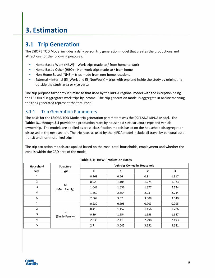
3.1 Trip Generation The LSIORB TOD Model includes a daily person trip generation model that creates the productions and
attractions for the following purposes:
Home Based Work (HBW) – Work trips made to / from home to work
Home Based Other (HBO) – Non work trips made to / from home
Non‐Home Based (NHB) – trips made from non‐home locations
External – Internal (EI_Work and EI_NonWork) – trips with one end inside the study by originating
outside the study area or vice versa
The trip purpose taxonomy is similar to that used by the KIPDA regional model with the exception being
the LSIORB disaggregates work trips by income. The trip generation model is aggregate in nature meaning
the trips generated represent the total zone.
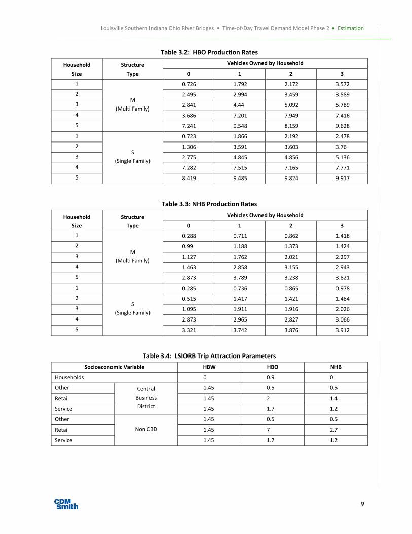
3.1.1 Trip Generation Parameters The basis for the LSIORB TOD Model trip generation parameters was the 09PLANA KIPDA Model. The
Tables 3.1 through 3.4 provide the production rates by household size, structure type and vehicle
ownership. The models are applied as cross‐classification models based on the household disaggregation
discussed in the next section. The trip rates as used by the KIPDA model include all travel by personal auto,
transit and non‐motorized trips.
The trip attraction models are applied based on the zonal total households, employment and whether the
zone is within the CBD area of the model.
Table 3.1: HBW Production Rates
Household
Size
Structure
Type
Vehicles Owned by Household
0 1 2 3
1
M
(Multi Family)
0.268 0.66 0.8 1.317
2 0.92 1.104 1.275 1.323
3 1.047 1.636 1.877 2.134
4 1.359 2.654 2.93 2.734
5 2.669 3.52 3.008 3.549
1
S
(Single Family)
0.232 0.598 0.703 0.795
2 0.419 1.152 1.156 1.206
3 0.89 1.554 1.558 1.647
4 2.336 2.41 2.298 2.493
5 2.7 3.042 3.151 3.181
Louisville Southern Indiana Ohio River Bridges • Time‐of‐Day Travel Demand Model Phase 2 Estimation
9
Table 3.2: HBO Production Rates
Household
Size
Structure
Type
Vehicles Owned by Household
0 1 2 3
1
M
(Multi Family)
0.726 1.792 2.172 3.572
2 2.495 2.994 3.459 3.589
3 2.841 4.44 5.092 5.789
4 3.686 7.201 7.949 7.416
5 7.241 9.548 8.159 9.628
1
S
(Single Family)
0.723 1.866 2.192 2.478
2 1.306 3.591 3.603 3.76
3 2.775 4.845 4.856 5.136
4 7.282 7.515 7.165 7.771
5 8.419 9.485 9.824 9.917
Table 3.3: NHB Production Rates
Household
Size
Structure
Type
Vehicles Owned by Household
0 1 2 3
1
M
(Multi Family)
0.288 0.711 0.862 1.418
2 0.99 1.188 1.373 1.424
3 1.127 1.762 2.021 2.297
4 1.463 2.858 3.155 2.943
5 2.873 3.789 3.238 3.821
1
S
(Single Family)
0.285 0.736 0.865 0.978
2 0.515 1.417 1.421 1.484
3 1.095 1.911 1.916 2.026
4 2.873 2.965 2.827 3.066
5 3.321 3.742 3.876 3.912
Table 3.4: LSIORB Trip Attraction Parameters
Socioeconomic Variable HBW HBO NHB
Households 0 0.9 0
Other Central
Business
District
1.45 0.5 0.5
Retail 1.45 2 1.4
Service 1.45 1.7 1.2
Other
Non CBD
1.45 0.5 0.5
Retail 1.45 7 2.7
Service 1.45 1.7 1.2
Louisville Southern Indiana Ohio River Bridges • Time‐of‐Day Travel Demand Model Phase 2 Estimation
10
3.1.2 Income Disaggregation of Households The LSIORB TOD Model includes a feature to estimate the number of trips generated by income group and
trip purpose. The disaggregation of trip purposes is carried through mode choice and traffic assignment.
The rationale for including an income dimension to the trip purposes is the following:
By including income in the HBW purpose, high income employment can be linked to high income
households, thus improving the trip distribution patterns in the model
Mode choice segments the market for transit by trip purpose by income. Income is used to
approximate auto availability and willingness to use transit for choice riders
The assignment model uses a generalized cost approach that includes operating cost and tolls in the
future. Segmenting trips by income allows for the testing of values of time that are based on income
groups
To apply the income based trip generation models it is necessary to add a fourth dimension to the existing
household disaggregation model applied by KIPDA. The existing KIPDA models disaggregate the zonal
households by dwelling type (multi‐family and single family), household size and vehicle ownership. This
results in the zonal total households be distributed into 40 categories.
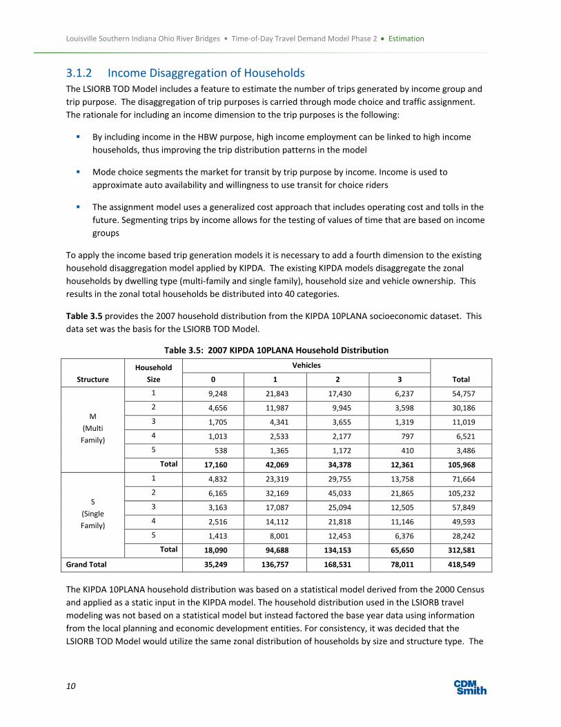
Table 3.5 provides the 2007 household distribution from the KIPDA 10PLANA socioeconomic dataset. This
data set was the basis for the LSIORB TOD Model.
Table 3.5: 2007 KIPDA 10PLANA Household Distribution
Structure
Household
Size
Vehicles
Total 0 1 2 3
M
(Multi
Family)
1 9,248 21,843 17,430 6,237 54,757
2 4,656 11,987 9,945 3,598 30,186
3 1,705 4,341 3,655 1,319 11,019
4 1,013 2,533 2,177 797 6,521
5 538 1,365 1,172 410 3,486
Total 17,160 42,069 34,378 12,361 105,968
S
(Single
Family)
1 4,832 23,319 29,755 13,758 71,664
2 6,165 32,169 45,033 21,865 105,232
3 3,163 17,087 25,094 12,505 57,849
4 2,516 14,112 21,818 11,146 49,593
5 1,413 8,001 12,453 6,376 28,242
Total 18,090 94,688 134,153 65,650 312,581
Grand Total 35,249 136,757 168,531 78,011 418,549
The KIPDA 10PLANA household distribution was based on a statistical model derived from the 2000 Census
and applied as a static input in the KIPDA model. The household distribution used in the LSIORB travel
modeling was not based on a statistical model but instead factored the base year data using information
from the local planning and economic development entities. For consistency, it was decided that the
LSIORB TOD Model would utilize the same zonal distribution of households by size and structure type. The

Louisville Southern Indiana Ohio River Bridges • Time‐of‐Day Travel Demand Model Phase 2 Estimation
11
income disaggregation would be based on applying a distribution to each of the existing household
disaggregation categories.
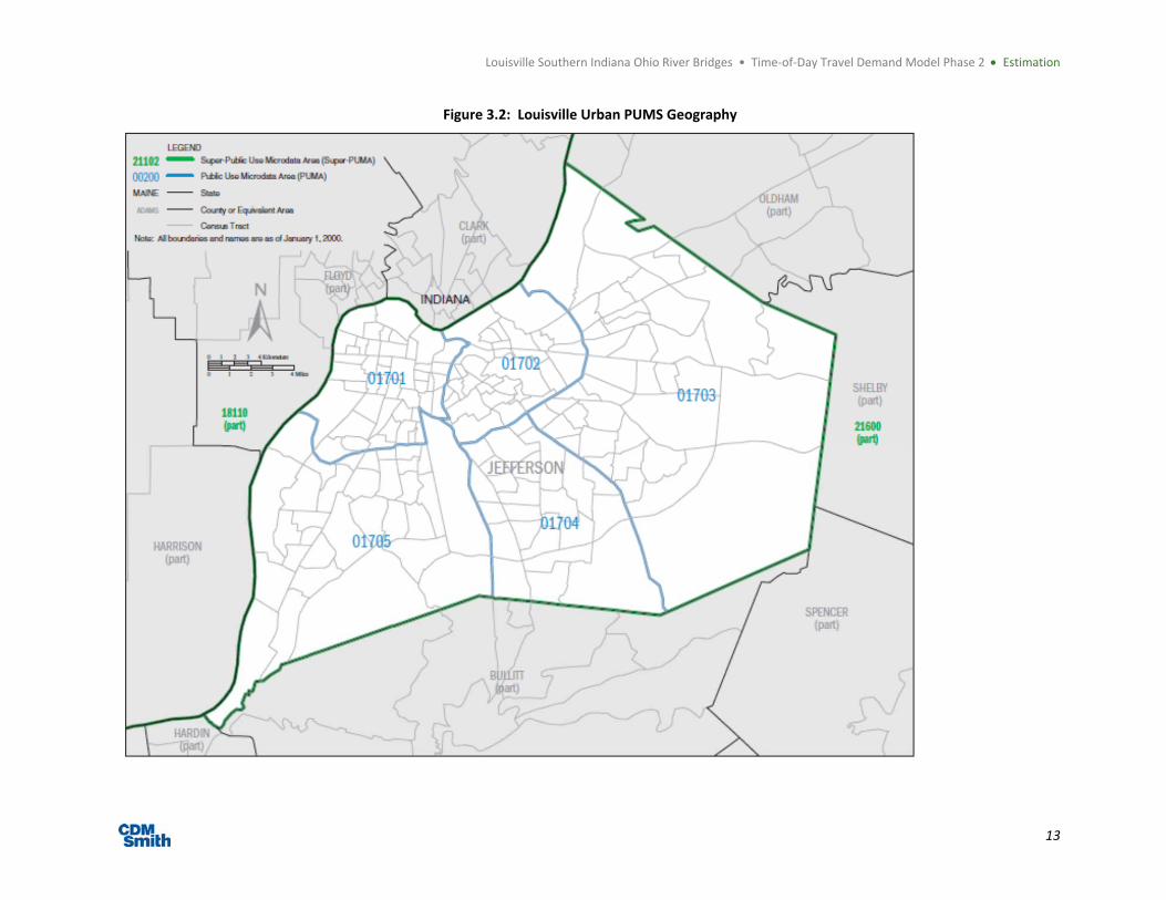
3.1.2.1 Definition of Income Categories
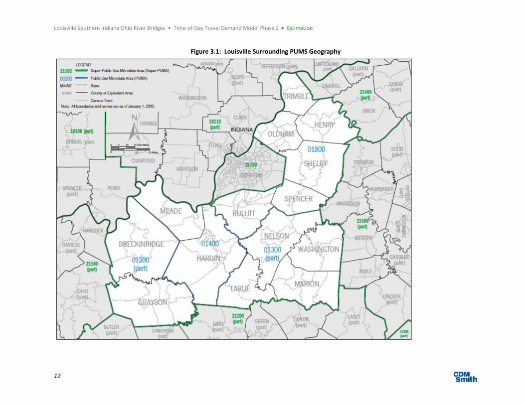
To define the income groupings, the Public Use Microdata (PUMS) was utilized from the 2000 Census. The
PUMS was utilized to because it includes not only the income of the household, but the NAICS of the
worker in each household as well. Using this information for each household it is possible to understand
the income distribution of households in the region, but also the associated employment types by income
group.
From Figure 3.1 , Figure 3.2, and Figure 3.3, the PUMS geography that covers the Louisville model area
were selected.
Louisville Southern Indiana Ohio River Bridges • Time‐of‐Day Travel Demand Model Phase 2 Estimation
12
Figure 3.1: Louisville Surrounding PUMS Geography
Louisville Southern Indiana Ohio River Bridges • Time‐of‐Day Travel Demand Model Phase 2 Estimation
13
Figure 3.2: Louisville Urban PUMS Geography

Louisville Southern Indiana Ohio River Bridges • Time‐of‐Day Travel Demand Model Phase 2 Estimation
14
Figure 3.3: Indiana PUMS Geography

Louisville Southern Indiana Ohio River Bridges • Time‐of‐Day Travel Demand Model Phase 2 Estimation
15
Based on the above geography, the distribution of households by total income was calculated and is shown
in Figure 3.4.
Figure 3.4: Distribution of Households by Income
From the above distribution several schemes were considered of how to aggregate the distribution data,
shown in Table 3.6. For consistency with the definition of income in other components of the EIS, it was
decided that three income groups would be defined: $0 to $40,000, $40,000 to $60,000 and greater than
$60,000.
Table 3.6: Number of Households by Income and Grouping
INC HH CUMTOT QUAR TRI
0 16791 16791 1 1
10000 52505 69296 1 1
20000 58535 127831 2 1
30000 60378 188209 2 1
40000 51332 239541 3 2
50000 47677 287218 3 2
60000 34417 321635 4 3
70000 28931 350566 4 3
80000 20641 371207 4 3
90000 13835 385042 4 3
100000 10721 395763 4 3
110000 8494 404257 4 3
120000 5871 410128 4 3
130000 4267 414395 4 3
140000 3335 417730 4 3
150000 19873 437603 4 3
0
20000
40000
60000
80000
100000
120000
140000
Number of Households
Household Annual Income
Distribution of Household by Income

Louisville Southern Indiana Ohio River Bridges • Time‐of‐Day Travel Demand Model Phase 2 Estimation
16
Using the three categories, the Census Tract data from 2000 was utilized to establish the distribution of
households in each Tract in the region. The region is represented by 230 census tracts as shown in Figure
3.5. The TAZs within the tract are assigned the income distribution of the tract. The income distribution is
then applied to each household category.
Figure 3.5: Louisville Region Census Tracts vs Traffic Analysis Zones
The resulting total household distribution by income group in 2007 is reported in Table 3.7.
Table 3.7: 2007 Household Distribution by Income
INC1 INC2 INC3 Total
Households 91166.2 108675.7 218707.2 418549.2
Distribution 21.8% 26.0% 52.3% 100.0%

Louisville Southern Indiana Ohio River Bridges • Time‐of‐Day Travel Demand Model Phase 2 Estimation
17
3.1.3 HBW by Income The trip generation model estimates a unique set of productions by purpose for each income group in the
model. For HBW, the model uses this information to link the household income to appropriate job types in
the region. To accomplish this, the distribution of the KIPDA employment types by household income was
required.
Using the PUMS data discussed in the previous section, the household income distribution of the NAICS
employment type was developed for the region. The resulting distribution is provided in Table 3.8.
Table 3.8: Distribution of Household Income by NAICS Employment
NAICS INCOME GROUP (PWEIGHT) INCOME GROUP (Percent)
2 DIGIT DESC. MODEL 1 2 3 1 2 3
11 AGR OTH 2901 1036 1472 53.6% 19.2% 27.2%
21 MINING OTH 411 203 398 40.6% 20.1% 39.3%
22 UTILITY OTH 1021 1366 3677 16.8% 22.5% 60.6%
23 CONST OTH 17793 11190 17236 38.5% 24.2% 37.3%
31 MANUF OTH 4745 4082 6739 30.5% 26.2% 43.3%
32 MANUF OTH 9901 7636 12836 32.6% 25.1% 42.3%
33 MANUF OTH 17229 15699 28844 27.9% 25.4% 46.7%
42 WHOLES RETAIL 7716 6782 11120 30.1% 26.5% 43.4%
44 RETAIL RETAIL 18991 11344 20262 37.5% 22.4% 40.0%
45 RETAIL RETAIL 10228 6039 8735 40.9% 24.2% 34.9%
48 TRANSP OTH 5886 4816 7099 33.1% 27.1% 39.9%
49 TRANSP OTH 6003 4987 8400 31.0% 25.7% 43.3%
51 INFO SERV 4246 3687 6981 28.5% 24.7% 46.8%
52 FININS SERV 9637 7431 17486 27.9% 21.5% 50.6%
53 REAL SERV 3240 2100 4781 32.0% 20.7% 47.2%
54 PROF SERV 7018 4157 16587 25.3% 15.0% 59.7%
55 MANG SERV 131 159 400 19.0% 23.0% 58.0%
56 ADM SERV 11558 5074 6556 49.8% 21.9% 28.3%
61 ED SERV 13299 10487 22970 28.4% 22.4% 49.1%
62 HEALTH SERV 26598 18751 34680 33.2% 23.4% 43.3%
71 ARTS SERV 5045 3352 4810 38.2% 25.4% 36.4%
72 ACCOM SERV 22045 10229 14703 46.9% 21.8% 31.3%
81 OTHER SERV 14367 8558 11975 41.2% 24.5% 34.3%
92 PUB SERV 7997 7460 11237 30.0% 27.9% 42.1%
99 1612 530 516 60.6% 19.9% 19.4%
Based on the relationship of each NAICS employment category to the categories used by KIPDA’s
socioeconomic dataset, a distribution was developed for each category (Table 3.9).
In application, the income group percentages are applied to each employment type and the attraction
coefficient for HBW trip attractions to calculate the income attractions.

Louisville Southern Indiana Ohio River Bridges • Time‐of‐Day Travel Demand Model Phase 2 Estimation
18
Table 3.9: Distribution of Employment by Model Income Variables
INCOME GROUP (PWEIGHT) INCOME GROUP (Percent)
Variable 1 2 3 1 2 3
OTH 65890 51015 86701 32.4% 25.1% 42.6%
RETAIL 36935 24165 40117 36.5% 23.9% 39.6%
SERV 125181 81445 153166 34.8% 22.6% 42.6%
3.1.4 HBO and NHB by Income The disaggregation of attractions is only applied to the HBW purposes. A different approach was taken to
accommodate the income disaggregation of the HBO and NHB trip purposes for mode choice and traffic
assignment.
For HBO trips, the disaggregation of the trips is performed post distribution to the PA format person trip
table. The income distribution of the zonal households is applied to the trip table row to create the income
1, 2 and 3 HBO trips. These trips are then used in mode choice. Because the home end of the trip is not
known for NHB trips, the regional distribution of income categories is applied to all zones to create the
three income NHB trip tables.
3.1.5 Special Generators and Trip Balancing The LSIORB TOD Model applies the same special generator methodology as used by the KIPDA model
including the location and magnitude of the special generators (Figure 3.6).

Louisville Southern Indiana Ohio River Bridges • Time‐of‐Day Travel Demand Model Phase 2 Estimation
19
Figure 3.6: 2007 LSIORB TOD Special Generators
The final step in the trip generation model is the balancing of the production and attractions. For HBW
trips, the income group attractions are balanced to the specific income productions. Because the income
disaggregation for HBO and NHB purposes are applied later in the model, the productions and attractions
are balanced in the typical method. This means for NHB trips, the attractions are adjusted to the total NHB
productions and then productions are set equal to attractions.
3.2 Network The LSIORB Phase II TransCAD network is a multi‐modal travel demand model network that includes
highway links as well as drive and walk access links to support the transit routes used in the mode choice
step.

Louisville Southern Indiana Ohio River Bridges • Time‐of‐Day Travel Demand Model Phase 2 Estimation
20
The LSIORB GISDK code populates the link attributes required for traffic assignment including the free flow
travel times, link capacities, alpha and beta parameters and the generalized cost for auto and truck
purposes.
3.2.1 Free Flow Speeds As part of the development of the LSIORB Phase II Model, CDM Smith has changed the free flow speed
logic from that used by KIPDA in the previous model. The free flow speed is a function of the following:
Posted speed limit
Default speeds in the absence of speed limits
Free flow adjustments
Signalization
3.2.1.1 Posted Speed Limit
The Kentucky Highway Information System was utilized to identify the posted speed limits on the state
maintained routes in the Kentucky portion of the study area (Figure 3.7). Similar information was not
made available from Indiana.

Louisville Southern Indiana Ohio River Bridges • Time‐of‐Day Travel Demand Model Phase 2 Estimation
21
Figure 3.7: Posted Speed Limits (Kentucky Highway Information System)
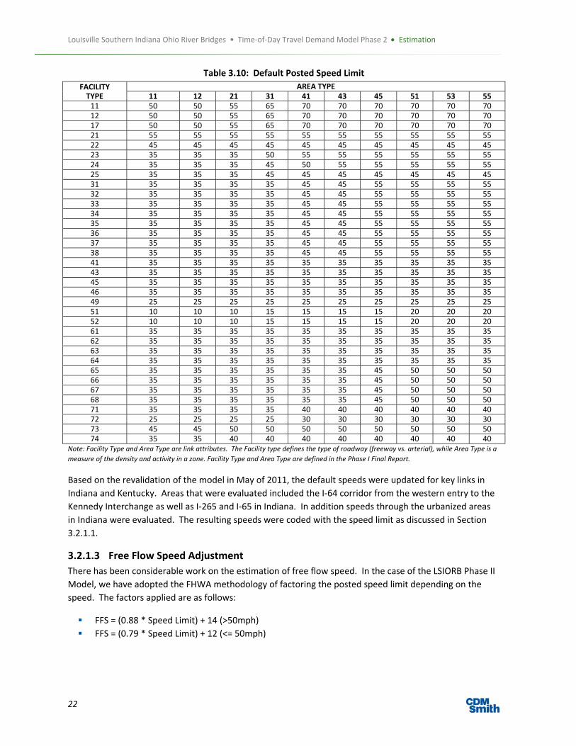
3.2.1.2 Default Speeds
The posted speed limit data was not complete, and it was necessary to develop default values for facilities
where posted speed limit data was not available. Using the links in the network with information, an
analysis was completed evaluating the typical posted speed limit by facility type and area type. Those
values were then used to populate the default speed table used in the model (Table 3.10). The LSIORB
Model scripts read the default values for links that do not have a posted speed limit attribute value.
Louisville Southern Indiana Ohio River Bridges • Time‐of‐Day Travel Demand Model Phase 2 Estimation
22
Table 3.10: Default Posted Speed Limit
FACILITY TYPE
AREA TYPE11 12 21 31 41 43 45 51 53 55
11 50 50 55 65 70 70 70 70 70 7012 50 50 55 65 70 70 70 70 70 7017 50 50 55 65 70 70 70 70 70 7021 55 55 55 55 55 55 55 55 55 5522 45 45 45 45 45 45 45 45 45 4523 35 35 35 50 55 55 55 55 55 5524 35 35 35 45 50 55 55 55 55 5525 35 35 35 45 45 45 45 45 45 4531 35 35 35 35 45 45 55 55 55 5532 35 35 35 35 45 45 55 55 55 5533 35 35 35 35 45 45 55 55 55 5534 35 35 35 35 45 45 55 55 55 5535 35 35 35 35 45 45 55 55 55 5536 35 35 35 35 45 45 55 55 55 5537 35 35 35 35 45 45 55 55 55 5538 35 35 35 35 45 45 55 55 55 5541 35 35 35 35 35 35 35 35 35 3543 35 35 35 35 35 35 35 35 35 3545 35 35 35 35 35 35 35 35 35 3546 35 35 35 35 35 35 35 35 35 3549 25 25 25 25 25 25 25 25 25 2551 10 10 10 15 15 15 15 20 20 2052 10 10 10 15 15 15 15 20 20 2061 35 35 35 35 35 35 35 35 35 3562 35 35 35 35 35 35 35 35 35 3563 35 35 35 35 35 35 35 35 35 3564 35 35 35 35 35 35 35 35 35 3565 35 35 35 35 35 35 45 50 50 5066 35 35 35 35 35 35 45 50 50 5067 35 35 35 35 35 35 45 50 50 5068 35 35 35 35 35 35 45 50 50 5071 35 35 35 35 40 40 40 40 40 4072 25 25 25 25 30 30 30 30 30 3073 45 45 50 50 50 50 50 50 50 5074 35 35 40 40 40 40 40 40 40 40
Note: Facility Type and Area Type are link attributes. The Facility type defines the type of roadway (freeway vs. arterial), while Area Type is a
measure of the density and activity in a zone. Facility Type and Area Type are defined in the Phase I Final Report.
Based on the revalidation of the model in May of 2011, the default speeds were updated for key links in
Indiana and Kentucky. Areas that were evaluated included the I‐64 corridor from the western entry to the
Kennedy Interchange as well as I‐265 and I‐65 in Indiana. In addition speeds through the urbanized areas
in Indiana were evaluated. The resulting speeds were coded with the speed limit as discussed in Section
3.2.1.1.
3.2.1.3 Free Flow Speed Adjustment
There has been considerable work on the estimation of free flow speed. In the case of the LSIORB Phase II
Model, we have adopted the FHWA methodology of factoring the posted speed limit depending on the
speed. The factors applied are as follows:
FFS = (0.88 * Speed Limit) + 14 (>50mph)
FFS = (0.79 * Speed Limit) + 12 (<= 50mph)

Louisville Southern Indiana Ohio River Bridges • Time‐of‐Day Travel Demand Model Phase 2 Estimation
23
3.2.1.4 Impact of Signalization
An additional enhancement to the LSIORB Phase II Model is the addition of capturing the uniform delay
from traffic signals as part of the free flow time. Extensive work was completed in Phase I and Phase II
identifying the locations of signals in the study area, and making assumptions regarding the cycle length. In
the end, several assumptions were made regarding the signal delay including:
Equal green time split by approach
Signal length based on known information and generalization for area type
No reduction in signal delay from progression
The delay related to signalization was calculated by direction on each link based on the location of the
signals. The formula used for estimating the uniform delay was:
The resulting delay was added to the free slow speed to develop the final adjusted free flow travel time.
3.2.2 Capacity Link level capacities are based on the look up table developed by KIPDA for the 09PlanA and 10PlanA
regional models. The capacity logic used by KIPDA is borrowed from FDOT and is based on accepted HCM
methodologies.
3.2.2.1 Daily Capacity from Existing Model
The KIPDA model is a daily model meaning it uses a daily assignment. As in most daily (24‐hour) models,
congested travel speed is used in the generalized cost computations and in capacity constraint during
traffic assignment. The congested speed is evaluated based on the peak hour of traffic within the period,
by comparing the peak hour volume to the hourly capacity. A factor is applied to convert between daily
volume and capacity and peak hour volume and capacity. In many daily models, this conversion is done in
advance by using a constant factor for the fraction of daily traffic that occurs during the peak hour. The
hourly capacity is then scaled up by that factor and compared directly to the daily volume estimated in the
model.
To maintain consistency with the existing daily model, it was decided that the capacities in the LSIORB TOD
Model would be based on the same data, which is represented as a “daily” capacity (hourly capacity
divided by the fraction of traffic occurring during the peak hour).
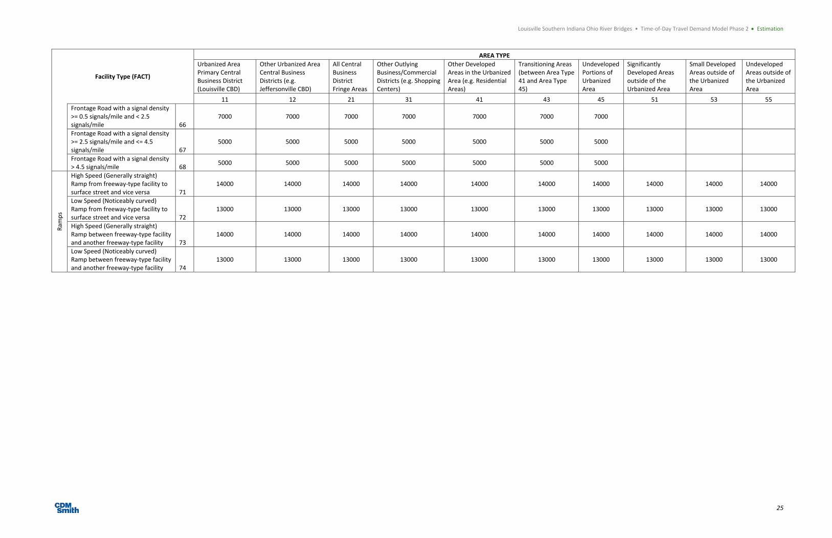
The source of the daily capacities in the KIPDA model is the 2009 Florida Quality / Level of Service
Handbook. KIPDA staff indicated they use the values for urbanized areas (Table 1, Chapter 5). The daily
per lane capacities from the existing model are shown in Table 3.11.

Louisville Southern Indiana Ohio River Bridges • Time‐of‐Day Travel Demand Model Phase 2 Estimation
24
Table 3.11. Existing KIPDA Daily Capacity per Lane (Source: 2000 KIPDA Model Plan09A)
Facility Type (FACT)
AREA TYPE
Urbanized Area Primary Central Business District (Louisville CBD)
Other Urbanized Area Central Business Districts (e.g. Jeffersonville CBD)
All Central Business District Fringe Areas
Other Outlying Business/Commercial Districts (e.g. Shopping Centers)
Other Developed Areas in the Urbanized Area (e.g. Residential Areas)
Transitioning Areas (between Area Type 41 and Area Type 45)
Undeveloped Portions of Urbanized Area
Significantly Developed Areas outside of the Urbanized Area
Small Developed Areas outside of the Urbanized Area
Undeveloped Areas outside of the Urbanized Area
11 12 21 31 41 43 45 51 53 55
Freeways 11 15000 15000 15000 15000 15000 15000 15000 15000 15000 15000
High‐Occupancy Vehicle Lanes 12 15000 15000 15000 15000 15000 15000 15000 15000 15000 15000
Collector ‐ Distributor Roads 17 15000 15000 15000 15000 15000 15000 15000 15000 15000 15000
Div Arterial
Divided Arterial with a signal density < 0.5 signals/mile and a speed limit of 55 miles per hour 21
8500 8500 8500 8500 8500 8500 8500 8500 8500 8500
Divided Arterial with a signal density < 0.5 signals/mile and a speed limit of 45 miles per hour 22
8500 8500 8500 8500 8500 8500 8500 8500 8500 8500
Divided Arterial with a signal density >= 0.5 signals/mile and < 2.5 signals/mile 23
7500 7500 7500 7500 7500 7500 7500 7500 7500 7500
Divided Arterial with a signal density >= 2.5 signals/mile and <= 4.5 signals/mile 24
7500 7500 7500 7500 7500 7500 7500 7500 7500 7500
Divided Arterial with a signal density > 4.5 signals/mile 25
6500 6500 6500 6500 6500 6500 6500 6500 6500 6500
UnDiv Arterial
Undivided Arterial with turning bays 31 6000 6000 6000 6000 7000 7000 7000 7000 7000 7000
Undivided Arterial without turning bays 35
5000 5000 5000 5000 6000 6000 6000 6000 6000 6000
Divided Collectors and Local Roads 41 5500 5500 5500 6000 6000 6000 6000 6000 6000 6000
Undivided Collectors and Local Roads 45
4500 4500 4500 4500 4500 4500 4500 4500 4500 4500
Side streets used for bus routes 49 2500 2500 2500 2500 2500 2500 2500 2500 2500 2500
CC Basic Centroid Connector 51 100000 100000 100000 100000 100000 100000 100000 100000 100000 100000
External Station Connector 52 100000
One Way
One‐Way Street with a signal density < 0.5 signals/mile 61
7000 7000 7000 7000 7000 7000 7000
One‐Way Street with a signal density >= 0.5 signals/mile and < 2.5 signals/mile 62
7000 7000 7000 7000 7000 7000 7000
One‐Way Street with a signal density >= 2.5 signals/mile and <= 4.5 signals/mile 63
5000 5000 5000 5000 5000 5000 5000
One‐Way Street with a signal density > 4.5 signals/mile 64
5000 5000 5000 5000 5000 5000 5000
on
tag Frontage Road with a signal density < 0.5 signals/mile 65
7000 7000 7000 7000 7000 7000 7000
Louisville Southern Indiana Ohio River Bridges • Time‐of‐Day Travel Demand Model Phase 2 Estimation
25
Facility Type (FACT)
AREA TYPE
Urbanized Area Primary Central Business District (Louisville CBD)
Other Urbanized Area Central Business Districts (e.g. Jeffersonville CBD)
All Central Business District Fringe Areas
Other Outlying Business/Commercial Districts (e.g. Shopping Centers)
Other Developed Areas in the Urbanized Area (e.g. Residential Areas)
Transitioning Areas (between Area Type 41 and Area Type 45)
Undeveloped Portions of Urbanized Area
Significantly Developed Areas outside of the Urbanized Area
Small Developed Areas outside of the Urbanized Area
Undeveloped Areas outside of the Urbanized Area
11 12 21 31 41 43 45 51 53 55
Frontage Road with a signal density >= 0.5 signals/mile and < 2.5 signals/mile 66
7000 7000 7000 7000 7000 7000 7000
Frontage Road with a signal density >= 2.5 signals/mile and <= 4.5 signals/mile 67
5000 5000 5000 5000 5000 5000 5000
Frontage Road with a signal density > 4.5 signals/mile 68
5000 5000 5000 5000 5000 5000 5000
Ram
ps
High Speed (Generally straight) Ramp from freeway‐type facility to surface street and vice versa 71
14000 14000 14000 14000 14000 14000 14000 14000 14000 14000
Low Speed (Noticeably curved) Ramp from freeway‐type facility to surface street and vice versa 72
13000 13000 13000 13000 13000 13000 13000 13000 13000 13000
High Speed (Generally straight) Ramp between freeway‐type facility and another freeway‐type facility 73
14000 14000 14000 14000 14000 14000 14000 14000 14000 14000
Low Speed (Noticeably curved) Ramp between freeway‐type facility and another freeway‐type facility 74
13000 13000 13000 13000 13000 13000 13000 13000 13000 13000

Louisville Southern Indiana Ohio River Bridges • Time‐of‐Day Travel Demand Model Phase 2 Estimation
26
3.2.2.2 Period Capacity
To develop period capacities for the LSIORB TOD Model, it is necessary to extract the hourly capacity from
the daily capacity tables, and to compute peak hour traffic in each of the periods evaluated in the model.
The TOD model has 8 periods:
AM Peak Period:
– 6am to 7am
– 7am to 8am
– 8am to 9am
Mid‐Day
– 9am to 3pm
PM Peak Period
– 3pm to 4pm
– 4pm to 5pm
– 5pm to 6pm
Overnight
– 6pm to 6am
For the peak periods, where the analysis period is a single hour, the daily capacity was converted to an
hourly capacity using a 10% K factor. That is, the daily capacities in the KIPDA capacity table were equated
to hourly capacities by multiplying the daily capacity by 10% (0.10). This practice is consistent with HCM
and with other daily models, and the resulting hourly capacities are reasonable.
For development of the mid‐day and overnight capacities, CDM Smith completed extensive research on the
state of the practice in performing peak hour volume and capacity conversions in several models (Table
3.12).

Louisville Southern Indiana Ohio River Bridges • Time‐of‐Day Travel Demand Model Phase 2 Estimation
27
Table 3.12. State of the Practice ‐ Period Capacities
Model Spreading PK
(am+pm) Source
Metrolina equal 6 Metrolina Model User's Manual, December 2007
Genesee County equal 6 Genese County Urban TDM Improvements: Model Development and Validation Report, May 2009
Fresno County equal 6 Fresno County Travel Demand Model 2003 Base, March 2010
H‐GAC equal 6 H‐GAC Model Validation and Documentation Report, February 2001
Bannock equal 2 Travel Demand Model 2006 Update: Travel Model Run Procedures for FY2007, February 2007
Rapid City equal 2 Rapid City TDM Documentation and User's Guide, March 2004
Triangle Region equal 4 Model Files
Asheville, NC equal 2 NCHRP Report 365, Case Study, 1998
Douglas County equal 2 Douglas County/Carson City Travel Demand Model: Final Report, May 2007
Charleston equal 6 Model Files
CAMPO equal 4 Model Files
Nashville equal 4 Model Files
FSUTMS n/a 0 FSUTMS‐Cube Framework Phase I: Default Model Parameters, Final Report, October 2006
Ohio Varied n/a Travel Demand Forecasting Manual 1: Traffic Assignment Procedures, August 2001
LCATS Varied 3 Travel Demand Forecasting Manual 1: Traffic Assignment Procedures, August 2001
Baltimore TDM equal 3 Baltimore Region Travel Demand Model, Version 3.3, Performance Check & Analysis for 2005, December 2007
Metropolitan Washington
equal 3 Summary of the State of the Practice and State of the Art of Modeling Peak Spreading, November 2007
Other n/a n/a Time of Day Modeling Procedures Report, TMIP
The result of the review indicated that standard practice is to multiply the hourly capacity times the
number of hours. This assumes a flat distribution of traffic across all hours in the period.
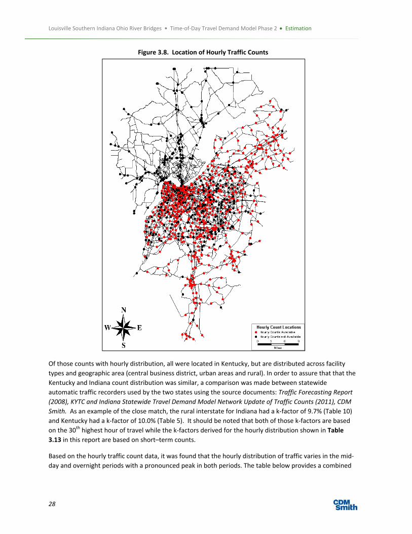
To identify whether this assumption was valid for LSIORB, an analysis of hourly traffic count data in the
region provided by INDOT and KYTC was completed. As documented in the Phase I Report, an extensive
effort was completed to identify all available count data in the region and populate that data to the LSIORB
2007 network. Counts were organized into a GIS database and included classification and hourly
distribution data when available. Figure 3.8 provides a map showing the location of the available counts
that included hourly distribution information. Of the over twelve hundred counts identified for validation,
slightly more than half (685) included data on the hourly distribution.
Louisville Southern Indiana Ohio River Bridges • Time‐of‐Day Travel Demand Model Phase 2 Estimation
28
Figure 3.8. Location of Hourly Traffic Counts
Of those counts with hourly distribution, all were located in Kentucky, but are distributed across facility
types and geographic area (central business district, urban areas and rural). In order to assure that that the
Kentucky and Indiana count distribution was similar, a comparison was made between statewide
automatic traffic recorders used by the two states using the source documents: Traffic Forecasting Report
(2008), KYTC and Indiana Statewide Travel Demand Model Network Update of Traffic Counts (2011), CDM
Smith. As an example of the close match, the rural interstate for Indiana had a k‐factor of 9.7% (Table 10)
and Kentucky had a k‐factor of 10.0% (Table 5). It should be noted that both of those k‐factors are based
on the 30th highest hour of travel while the k‐factors derived for the hourly distribution shown in Table
3.13 in this report are based on short–term counts.
Based on the hourly traffic count data, it was found that the hourly distribution of traffic varies in the mid‐
day and overnight periods with a pronounced peak in both periods. The table below provides a combined

Louisville Southern Indiana Ohio River Bridges • Time‐of‐Day Travel Demand Model Phase 2 Estimation
29
hourly distribution of counts in the study area. Within the overnight period, the distribution varies from
over 5% of the daily volume to less than 1 percent. In the mid‐day, the distribution varies as well.
Table 3.13. Hourly Distribution of Traffic
Hour Percent Period
Midnight ‐ 1am 1.02%
5.78%
1am ‐ 2am 0.67%
2am ‐ 3am 0.56%
3am ‐ 4am 0.61%
4am ‐ 5am 0.92%
5am ‐ 6am 2.00%
6am ‐ 7am 4.33%
18.01% 7am ‐ 8am 7.16%
8am ‐ 9am 6.51%
9am ‐ 10am 5.11%
32.56%
10am ‐ 11am 4.83%
11am – Noon 5.16%
Noon ‐ 1pm 5.52%
1pm ‐ 2pm 5.61%
2pm ‐ 3pm 6.34%
3pm ‐ 4pm 7.11%
22.86% 4pm ‐ 5pm 7.76%
5pm ‐ 6pm 7.99%
6pm ‐ 7pm 5.83%
20.78%
7pm ‐ 8pm 4.34%
8pm ‐ 9pm 3.62%
9pm ‐ 10pm 3.02%
10pm ‐ 11pm 2.32%
11pm – Midnight 1.65%
Because of the large variation of traffic during the mid‐day and overnight hours it was determined that a
factor should be used that better represents the analysis period. A method was developed to determine
these factors based on a similar approach to estimating a daily capacity as used by KIPDA. The approach
used was applied to the mid‐day and overnight periods by using the ratio of the period total traffic to the
peak hour traffic within that period.
The percent of traffic in mid‐day and overnight periods was identified. For the mid‐day, this was
found to be 32.56 percent and 26.56 for overnight.
The percent of traffic in the peak hour of the period was also identified. The highest mid‐day hour
was observed between 2 and 3pm and was 6.34% of the daily traffic. For overnight, the highest hour
was 6 to 7pm and was 5.83% of the day.
The percent of traffic occurring in the highest hour for the period was calculated:
– Mid‐day: 32.56/6.34 = 5.14
– Overnight: 26.56/5.83 = 4.55
The resulting factor for the mid‐day and overnight, shown in Table 3.14, were then used to compare the
peak hour of traffic in the period to the hourly capacity as determined by the link facility type.

Louisville Southern Indiana Ohio River Bridges • Time‐of‐Day Travel Demand Model Phase 2 Estimation
30
Table 3.14. Period Peak Hour Volume Calculation
Assignment Period Hours Peak Hour Volume
Mid‐Day 9am to 3pm Period Volume / 5.14
Overnight 6pm to 6am Period Volume / 4.55
AM Peak: First Hour 6am to 7am
Period Volume / 1.0
AM Peak: Second Hour 7am to 8 am
AM Peak: Third Hour 8 am to 9am
PM Peak: First Hour 3pm to 4 pm
PM Peak: Second Hour 4pm to 5 pm
PM Peak: Third Hour 5pm to 6pm
The resulting effective period volumes are higher than if a uniform hourly factor were used. The advantage
to this approach is that congestion observed in the off peak periods in the region is better represented in
the model and considered in the route choice in traffic assignment.
For computational efficiency during the assignment process, the capacity was multiplied by the peak hour
volume factor rather than the volume divided by the factor. (The volume‐to‐capacity ratio, which is what
the model uses to evaluate congestion, is numerically the same in either case). Based on the above
information, an example calculation for per lane capacity for the periods is as follows:
Daily Capacity = 15000 (daily per lane capacity for freeway in CBD)
Peak Hour Capacity = 1500 (hourly capacity, used in AM and PM hourly assignments)
Mid‐Day Capacity = 1500 * 5.14 (effective period capacity, used in Mid Day assignment)
Overnight Capacity = 1500 * 4.55 (effective period capacity, used in Overnight assignment)
The resulting peak hour volume‐to‐capacity ratios within each period are used in the assignment process
for the calculation of congested travel times. As described elsewhere in this report, the congested travel
times are then fed back to distribution and mode choice in combination with the other cost components of
travel.
3.2.3 Generalized Cost Impedance Most travel demand models utilize travel time impedance for the trip distribution step where trip
productions and attractions are used to generate the number of trips between origins and destinations.
This approach assumes travelers will prefer shorter travel times over longer ones. Since the LSIORB model
is to be used for modeling the effect of tolling which can cause trips to route on longer paths to avoid tolls,
the trip distribution impedance was augmented to include both time and distance based vehicle operating
costs. As noted in section 3.4.4., consistent values of time, vehicle operating costs, and toll costs, if
applicable, were also used in the mode choice step. In the trip assignment step where trips are assigned to
specific routes between origin and destination, a generalized cost function was used to account for all
three components of route choice: time, distance, and toll cost, if applicable. The generalized cost function
expresses the cost of the trips in terms of money (dollars) then assumes users will seek the lowest cost
route.
Time is monetized by assuming a value of time per minute and is distinct for car and truck trips. Distance is
monetized by assuming a vehicle operating cost per mile and, again, is distinct for car and truck trips.
Finally, the model allows tolls (which are already expressed as money) to be added in where a specific trip
will travel on a tolled facility in a specific scenario. Consequently, it is important to set appropriate values

Louisville Southern Indiana Ohio River Bridges • Time‐of‐Day Travel Demand Model Phase 2 Estimation
31
of time (VOT) and vehicle operating costs (VOC) to be used in the model. For traffic and revenue estimates
at the SEIS planning level, it is appropriate to use area socioeconomic data, national travel planning data,
and fundamental research on these topics to select appropriate values of time and vehicle operating costs.
3.2.3.1 Values of Time
It is important that the VOT not be assigned too high for this study. A high VOT can result in too little
diversion to alternate facilities resulting in underestimation of impacts on these facilities as well as over
estimation of tolling financial capacity. VOT for personal trips in passenger vehicles is generally considered
to be about 50% of the driver’s wage rate.1, 2 However, it has been noted that this percentage can vary
greatly from 35%‐60% of wage rate for personal local travel and 80‐120% for local business travel.3 For
intercity travel, these percentages can be higher. Due to the range of plausible VOT as a proportion of
income, the selection of a percentage of median wage for value of time is subjective. Although 50% for
personal trips is cited by many sources, higher levels are recommended for business or interstate travel by
car, but no general agreement exists on what this amount should be. A portion of car trips in the model
region and crossing the bridges are business trips and/or interstate trips. While there is no direct measure
available of business and/or interstate trips crossing the bridges, based on the SEIS model trip table, about
15% of the entire region’s trips are non‐home‐based trips (either for work or personal business) and about
12% of trips are to/from outside the region to the region or pass through the region. Without additional
detailed travel survey information, the proportion of these trips that can be considered business and/or
interstate trips that are at a high value of time cannot be precisely estimated. Consequently, to be
conservative, it was assumed approximately 10% of car trips are business and/or long distance and the
value of time for these trips is 100% of income. This assumption results in a weighted blended car trip VOT
of 55% of income.
For this study, socio‐economic data available from the US census regarding household income, number of
households, and number of hours worked covering the five‐county greater Louisville area were used to
calculate an appropriate VOT for automobiles. Table 3.15 and Table 3.16 derive the VOT for passenger cars
using information from the 2000 Census and 2010 American Community Survey (three year estimates)
covering the five counties included in the project model and the weighted average factor noted above.
1 Concas, Sisinnio and Kolpakov, Alexander, Synthesis of Research on Value of Time And Value of Reliability, Center for Urban Transportation Research, Florida Department of Transportation, January 2009. 2 Belenky, Peter and Trottenberg, Polly, Revised Departmental Guidance on Valuation of Travel Time in Economic Analysis, US Department of Transportation memo, September 28, 2011. 3 Ibid.

Louisville Southern Indiana Ohio River Bridges • Time‐of‐Day Travel Demand Model Phase 2 Estimation
32
Table 3.15. VOT Analysis Based On 2000 Census
County
House holds
Pop.16 and over
Median HH In
come
(1999$)
Total H
ours
Worked All
Workers M
illions)
Hours W
orked per
HH
HH In
come Per
Hour Worked
HH In
come Per
Minute W
orked
Weight Factor for
VOT
VOT per minute
(1999$)
CPI A
djust to
2010$
VOT per minute
(2010$)
Clark County, IN 38,774 75,843 $40,111 93.591 2414 $17 $0.28 0.55 $0.15 1.29 $0.20
Floyd County, IN 27,532 54,508 $44,022 66.541 2417 $18 $0.30 0.55 $0.17 1.29 $0.22
Bullitt County, KY 22,248 46,491 $45,106 57.749 2596 $17 $0.29 0.55 $0.16 1.29 $0.21
Jefferson County, KY 287,133 543,567 $39,457 625.974 2180 $18 $0.30 0.55 $0.17 1.29 $0.21
Oldham County, KY 14,846 35,002 $63,229 41.798 2815 $22 $0.37 0.55 $0.21 1.29 $0.27
Weighted VOT (by hours worked) $0.21
Table 3.16. VOT Analysis Based On 2010 3 Year American Community Survey Data
County
House holds
Pop.16 and over
Median HH In
come
(2009$)
Total H
ours
Worked All Workers
(Millions)
Hours W
orked per HH
HH In
come Per Hour
Worked
HH In
come Per
Minute W
orked
Weight Factor for VOT
VOT per minute (2009$)
CPI A
djust to 2010$
VOT per minute (2010$)
Clark County, IN 44,248 72,245 $48,046 96.766 2187 $22 $0.37 0.55 $0.20 1.02 $0.20
Floyd County, IN 29,479 49,266 $50,339 65.758 2231 $23 $0.38 0.55 $0.21 1.02 $0.21
Bullitt County, KY 27,673 49,504 $50,775 62.933 2274 $22 $0.37 0.55 $0.20 1.02 $0.21
Jefferson County, KY 309,175 485,306 $44,638 616.820 1995 $22 $0.37 0.55 $0.21 1.02 $0.21
Oldham County, KY 19,431 39,642 $81,755 47.015 2420 $34 $0.56 0.55 $0.31 1.02 $0.32
Weighted VOT (by hours worked) $0.21
Both sets of calculations in the tables above show very similar results of $0.21 per minute for car trips. To
further check the validity of this assumption, it was checked against other sources. For all local travel
purposes, the USDOT4 recommended value of time is $12.71 per hour (converted to 2010$) which is
equivalent to $0.21 per minute. Based on the demographically derived estimate for the study area
counties, $0.21 was used for automobile value of time for the SEIS analysis.
4 Ibid.

Louisville Southern Indiana Ohio River Bridges • Time‐of‐Day Travel Demand Model Phase 2 Estimation
33
Determining an appropriate VOT for trucks is even more complicated than for cars. Many different studies
have been conducted over time. Some generally consider time based operating costs such as driver wages
and benefits as a direct measure of truck VOT.5 6 However, other studies7 8 9 suggest the VOT exceeds
driver costs due to many factors affecting business economics including time‐value of freight. (Some
trucks carry freight that needs to be delivered by a specific time while others are not as time sensitive.)
Truck VOT is, consequently, very subjective and no agreement exists among the sources consulted. USDOT
(Belenky and Trottenberg) recommends a truck driver value of time of $25.11 with a plausible range
between $20.12 and $30.09 (adjusted to 2010$) based on wage rates. The American Transportation
Research Institute10 suggests the driver‐based costs (wages and benefits) are approximately $25.36
(adjusted to 2010$) per hour. Smalkoski and Levinson suggest a much higher value of $57.60 (adjusted to
2010$) and the American Transportation Research Institute suggests a range of $25 to $200 per hour
(unadjusted), which accounts for the driver pay and benefits as well as time value of freight. Given that the
model covers a large region with several interstate routes which use the Ohio River bridges, it was assumed
that at least some of the truck traffic has time‐value freight. Without additional area‐specific research and
surveys, an assumption must be made. A commercial vehicle VOT of $33.00 per hour, or $0.55 per minute,
was selected. This value reflects the wage and benefits based value of time of approximately $25, plus an
additional $8 (or 33%) to account for an average time‐value of freight per truck.
3.2.3.2 Vehicle Operating Costs
It is important that the vehicle operating costs (VOC) not be assumed too high for this study. A high VOC
can result in too little diversion to alternate facilities resulting in underestimation of impacts as well as over
estimation of financial capacity of tolling. Vehicle operating costs need to reflect that part of total vehicle
operating costs a driver would take into account when making a routing decision. Consequently, it is
generally assumed that fixed costs such as vehicle capital and insurance costs are not included, and vehicle
operating costs are comprised of variable costs such as fuel and wear‐and‐tear. In some of the studies
reviewed, vehicle operating costs may also include a portion of depreciation costs, which can be
considered both mileage and vehicle age based.
For automobiles, baseline information from the American Automobile Association is available11 that
indicates per mile operating costs (including fuel, maintenance, and tires) are $0.1674 for cars, $0.2231 for
SUVs, and $0.1931 for minivans. In 2003, Minnesota DOT commissioned a study12 which attempted to
calculate the per mile operating costs exclusive of the annual costs but including depreciation. Using the
results of this study, if the fuel costs are brought up to actual 2010 fuel costs (as reported by the US
Department of Energy, Midwest region), and repair, tires, and depreciation are brought to 2010$ using CPI
factors, the average passenger car VOC is $0.226 per mile. After reviewing the above data points, CDM
5 Ibid. 6 Concas and Kolpakov 7 Smalkoski and Levinson, Value of Time for Commercial Vehicle Operators in Minnesota, University of Minnesota, December, 2003. 8 Measuring Travel Time in Freight‐Significant Corridors, American Transportation Research Institute, FHWA, USDOT, 2005. 9 Kawamura, Kazuya, Commercial Vehicle Value of Time and Perceived Benefit of Congestion Pricing, University of California, Berkeley, 1999. 10 An Analysis of the Operational Costs of Trucking, American Transportation Research Institute, December, 2008, Table 4. 11 Your Driving Costs, AAA, 2010 edition. 12 Barnes, Gary and Langworthy, Peter, The Per‐mile Costs of Operating Automobiles and Trucks, University of Minnesota, June, 2003, Table 4.2, page 22.

Louisville Southern Indiana Ohio River Bridges • Time‐of‐Day Travel Demand Model Phase 2 Estimation
34
Smith selected an automobile average VOC of $0.19 per mile for this study which falls slightly below the
average of the values noted above.
Using the 2003 MnDOT modified methodology, a similar calculation showed commercial truck vehicle
operating cost of $0.608 per mile (2010$) including depreciation. The American Transportation Research
Institute13 shows a marginal VOC of $0.83 per mile (adjusted to 2010$) not including depreciation. After
adding in truck/trailer lease or purchase payments, this figure rises to $1.04. Both methods include fuel
and fuel taxes, repair and maintenance, and tires. Both studies cited above primarily covered 4‐5 axle
Tractor/Semitrailer heavy truck combinations. However, the SEIS model only includes a single combined
truck class for both light and heavy trucks. Consequently, the SEIS study assumes a breakout of 38% light
trucks and 62% heavy trucks for Ohio River crossings based on 2010 classification counts. Light trucks often
have higher gas mileage and lower maintenance costs resulting in lower VOC vs. heavy trucks.14
Considering the assumed proportion of light and heavy trucks and the information available, CDM Smith
chose a value of $0.65 per mile for overall truck vehicle operating costs, closer to the lower end of the
range of rates.
3.2.3.3 Cost Components
Based on the analysis above, Table 3.17 highlights the VOT and VOC values that are used in the LSIORB
Project TOD Model.
Table 3.17. VOT and VOC Values Used in LSIORB TOD Model (2010$)
Cars Trucks
Value of Time (VOT) $0.21 per minute $0.55 per minute
Vehicle Operating Cost (VOC) $0.19 per mile* $0.65 per mile
*Note that current federal per mile cost reimbursement is $0.51 per mile. The VOC cited in Table 3 above reflects only
those costs a driver would take into account when making a routing decision. The fixed costs of a vehicle such as insurance
are not included in the VOC values used in the model.
The LSIORB network has unique toll fields allowing the toll rates to be specified by peak period verses mid‐
day, by car occupancy, and by class (cars, light trucks, and heavy trucks). For purposes of this study,
however, tolls were assumed to be the same for single occupant and multi‐occupant cars. Tolls were
assumed to be the same for all trucks since only a single truck table was used. Tolling by time of day period
was considered, but the SEIS scenario uses a flat toll rate by class throughout the day. The tolls should be
coded at the toll collection location in dollars. The model combines the appropriate operating cost with
the toll value and inputs this into the generalized cost function at the appropriate steps in the model. The
Generalized Cost is calculated for all links based on the operating cost and adds the toll value for only the
links with a toll cost added as a link attribute.
3.2.3.4 Mode Choice VOT
As described in previously in this report, the mode choice structure and coefficients applied in the LSIORB
TOD Model were borrowed from another region as is common practice for areas without the necessary
data to estimate a new mode choice model. The borrowed model is from an area with a similar population
and transit service levels. In the review of the model coefficients prior to application in the LSIORB TOD
Model, it was found that the implied VOT was different from the VOT assumptions being used for trip
distribution and traffic assignment.
13 An Analysis of the Operational Costs of Trucking, American Transportation Research Institute, December, 2008, Table 4. 14 Barnes and Langworthy.Table 3.2, page 19.

Louisville Southern Indiana Ohio River Bridges • Time‐of‐Day Travel Demand Model Phase 2 Estimation
35
The implied value of time in mode choice is based on dividing the in vehicle travel time coefficient by the
cost coefficient. In the case of the borrowed values, the implied value of time was $12.50 for non‐work and
$6.53 for work trips. These values translate to $.208 per minute for non‐work and $.109 for work. The VOT
for the LSIORB TOD Model is $.21 per minute and is applied to work and non‐work trips in trip distribution
and traffic assignment.
Because it was not feasible to re‐estimate the mode choice model for the LSIORB TOD Model, a sensitivity
analysis was completed by adjusting the cost coefficients so that the implied value of time was consistent
with the VOT used in other model steps. Two runs were completed:
MCT: Implied VOT for work and non‐work purposes set to $.21 per minute
MCE: Implied VOT for work set to twice the non‐work VOT of $.21 per minute
Table 3.18 reports the total mode share for person trips for two sensitivity runs compared to the output of
the validated model for 2007.
Table 3.18. Mode Share for Person Trips Sensitivity Analysis
Mode 2007 Validation
Work and Non Work
Equal VOT
Work Twice
Non Work VOT
DA 39.3% 39.3% 39.3%
SR2 44.8% 44.8% 44.8%
SR3 5.7% 5.7% 5.7%
Local 1.3% 1.3% 1.3%
Prem 0.2% 0.2% 0.2%
Walk 6.6% 6.6% 6.6%
Bike 2.1% 2.1% 2.1%
Total 100.0% 100.0% 100.0%
When looking at the distribution by mode by purpose, the results show that there is no difference when
changing the cost coefficient for consistency with the implied value of time.
2007 Validation Auto Transit NM
HBW 92.3% 4.3% 3.4%
HBO 88.9% 0.8% 10.4%
NHB 90.2% 0.7% 9.1%
Total 89.8% 1.5% 8.7%
Work and Non Work
Equal VOT Auto Transit NM
HBW 92.3% 4.3% 3.4%
HBO 88.9% 0.8% 10.4%
NHB 90.2% 0.7% 9.1%
Total 89.8% 1.5% 8.7%

Louisville Southern Indiana Ohio River Bridges • Time‐of‐Day Travel Demand Model Phase 2 Estimation
36
Work Twice
Non Work VOT Auto Transit NM
HBW 92.3% 4.3% 3.4%
HBO 88.9% 0.8% 10.4%
NHB 90.2% 0.7% 9.1%
Total 89.8% 1.5% 8.7%
A sensitivity test was completed using the LSIORB TOD Model where the implied value of time in the mode
choice model was set equal to the value used for trip distribution and traffic assignment. The outcome of
that test showed very little change in the resulting mode shares in the model. This indicates that the cost
coefficients have little relative impact which is consistent with a captive ridership market.
3.3 Trip Distribution The LSIORB utilizes a traditional gravity model formulation for the trip distribution step in the model.
Enhancements to the typical gravity model include the following elements:
Use of a generalized cost function for impedance
Implementation of feedback to account for congestion in trip distribution
3.3.1 Friction Factor Calibration Because of the difference in definition of impedance in the LSIORB TOD Model and the use of a congested
feedback model, the friction factors had to be estimated. The 2000 KIPDA household travel survey was
used. Since the 2000 survey used the 1990 traffic analysis zones, the first step was to equate the trip ends
to the new zone structure. Once that step was complete, the composite congested time was assigned to
each survey trip and an average value was computed from the survey as well as the distribution of trips
over time. The congested travel time was based on preliminary runs of the model.
The friction factors were iteratively estimated by comparing the output trip length distribution to the
survey output and adjustments were made. A curve was then fit to the adjusted friction factors and the
model was rerun. This process was completed until the average values from the survey were replicated
within 10% or a difference of less than 2 minutes.
Figure 3.9 provides a comparison of the survey and estimated model average composite travel times by
purpose at the end of the calibration process. Figure 3.10, Figure 3.11, and Figure 3.12 display the
distribution from the survey (_S) and the calibrated model (_M) by purpose.

Louisville Southern Indiana Ohio River Bridges • Time‐of‐Day Travel Demand Model Phase 2 Estimation
37
Figure 3.9: Survey vs. LSIORB TOD Model: Average Composite Time
Figure 3.10: Survey vs. LSIORB TOD Model: HBW Composite Time Distribution
0
5
10
15
20
25
30
35
40
HBW HBO NHB
SURVEY
MODEL
0
0.5
1
1.5
2
2.5
3
1
11
21
31
41
51
61
71
81
91
101
111
121
131
141
151
161
Percent of Trips
Generalized Cost (Time + Cost / VOT)
HBW_S
HBW_M

Louisville Southern Indiana Ohio River Bridges • Time‐of‐Day Travel Demand Model Phase 2 Estimation
38
Figure 3.11: Survey vs. LSIORB TOD Model: HBO Composite Time Distribution
Figure 3.12: Survey vs. LSIORB TOD Model: NHB Composite Time Distribution
0
1
2
3
4
5
6
1
10
19
28
37
46
55
64
73
82
91
100
109
118
127
136
145
154
163
Percent of Trips
Generalized Cost (Time + Cost / VOT)
HBO_S
HBO_M
0
1
2
3
4
5
6
1
10
19
28
37
46
55
64
73
82
91
100
109
118
127
136
145
154
163
Percent of Trips
Generalized Cost (Time + Cost / VOT)
NHB_S
NHB_M

Louisville Southern Indiana Ohio River Bridges • Time‐of‐Day Travel Demand Model Phase 2 Estimation
39
Based on the observed and modeled distributions, the coincidence ratio was calculated for each purpose
(Table 3.19). The coincidence ratio, a measure recommended by the TMIP Model Validation and
Reasonableness Checking Manual, is a measure of the difference between two distributions. A value of 1.0
implies the distributions are the same.
Table 3.19: Trip Distribution Calibration Results
Purpose Observed Average Model Average Coincidence Ratio
HBW 33.77681 33.16751 0.836225
HBO 19.37822 19.88649 0.818359
NHB 19.65853 17.87851 0.813566
Note: Observed Average and Model Average are average trip length in minutes for the generalized cost function (time + cost / vot)
The resulting friction factors are shown Figure 3.13. The relative relationship between the trip purposes is
consistent with the expected response to travel time by trip purpose. HBW has a higher willingness to
travel as seen in the shallow slope of the curve as compared to HBO and NHB that fall off quickly.
Figure 3.13: LSIORB TOD Friction Factors
3.3.2 Feedback The LSIORB model uses feedback procedures to “feedback” congested travel times into the modeling
process. This is to ensure that inputs into earlier steps of the model are consistent with the model outputs
at later stages.
The purpose of a feedback mechanism is to make use of more accurate times from the assignment stage
into the earlier stages (trip distribution, mode choice, and time of day), and loop this way iteratively until
there is more consistency between the time values being used for each of the model stages. Figure 3.14
shows a flowchart of the feedback process.
0
500
1000
1500
2000
2500
1 7
13
19
25
31
37
43
49
55
61
67
73
79
85
91
97
Friction Factor value
Composite Time
HBW
HBO
NHB
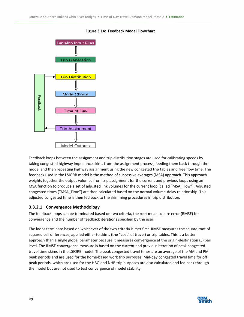
Louisville Southern Indiana Ohio River Bridges • Time‐of‐Day Travel Demand Model Phase 2 Estimation
40
Figure 3.14: Feedback Model Flowchart
Feedback loops between the assignment and trip distribution stages are used for calibrating speeds by
taking congested highway impedance skims from the assignment process, feeding them back through the
model and then repeating highway assignment using the new congested trip tables and free flow time. The
feedback used in the LSIORB model is the method of successive averages (MSA) approach. This approach
weights together the output volumes from trip assignment for the current and previous loops using an
MSA function to produce a set of adjusted link volumes for the current loop (called “MSA_Flow”). Adjusted
congested times (“MSA_Time”) are then calculated based on the normal volume‐delay relationship. This
adjusted congested time is then fed back to the skimming procedures in trip distribution.
3.3.2.1 Convergence Methodology
The feedback loops can be terminated based on two criteria, the root mean square error (RMSE) for
convergence and the number of feedback iterations specified by the user.
The loops terminate based on whichever of the two criteria is met first. RMSE measures the square root of
squared cell differences, applied either to skims (the “cost” of travel) or trip tables. This is a better
approach than a single global parameter because it measures convergence at the origin‐destination (ij) pair
level. The RMSE convergence measure is based on the current and previous iteration of peak congested
travel time skims in the LSIORB model. The peak congested travel times are an average of the AM and PM
peak periods and are used for the home‐based work trip purposes. Mid‐day congested travel time for off
peak periods, which are used for the HBO and NHB trip purposes are also calculated and fed back through
the model but are not used to test convergence of model stability.
Develop Input Files
Trip Generation
Trip Distribution
Mode Choice
Time of Day
Trip Assignment
Model Outputs
Feedb
ack

Louisville Southern Indiana Ohio River Bridges • Time‐of‐Day Travel Demand Model Phase 2 Estimation
41
3.3.2.2 Convergence Criteria
The measure of convergence can be set by the model user but a default value was chosen to be less than
to 0.1 RMSE. Caliper recommends a convergence threshold of 0.1 percent of RMSE between the current
and previous loops’ travel time skims. This measure is suggested to be detailed enough to appropriately
measure convergence. The LSIORB model convergence was tested based on this threshold and the model
converged in six feedback iterations.
By default the maximum number of feedback iterations is set to 100 in the LSIORB model but can be
adjusted by the user. Figure 3.15 and Table 3.20 show the number of feedback iterations verse the RMSE.
The model reaches the 0.1 RMSE threshold at iteration six but becomes fairly stable starting at iteration
four and little benefit is obtained after the fourth iteration in the 2007 model. Thus, iterations after the
fourth may not warrant the additional time sacrificed for the minimal convergence improvements.
Figure 3.15: Feedback Convergence Plot
0
10
20
30
40
2 3 4 5 6
RMSE
Iterations
Convergence
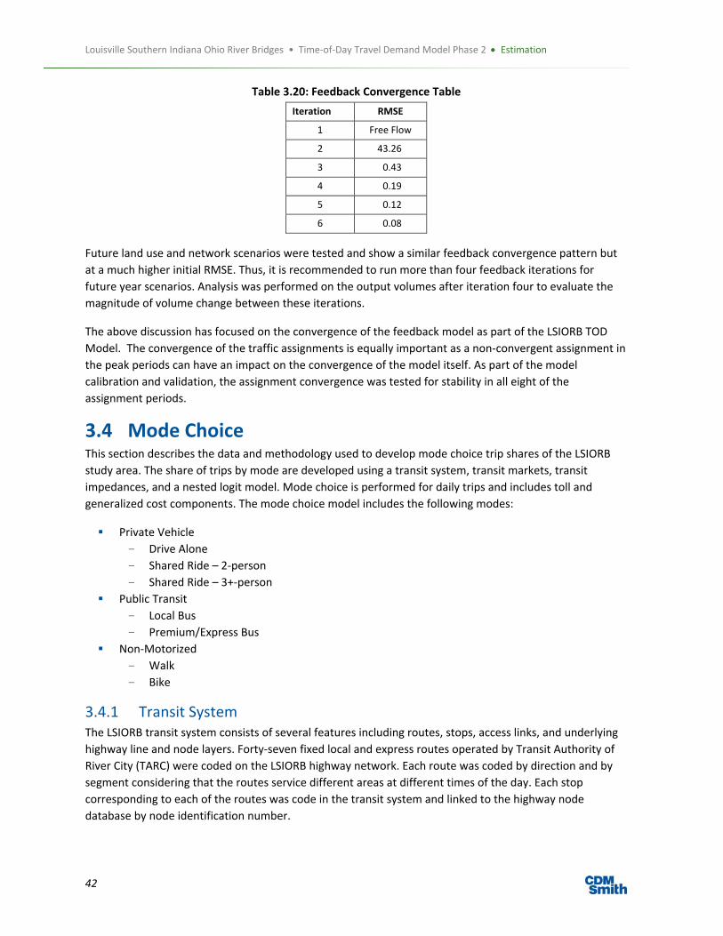
Louisville Southern Indiana Ohio River Bridges • Time‐of‐Day Travel Demand Model Phase 2 Estimation
42
Table 3.20: Feedback Convergence Table
Iteration RMSE
1 Free Flow
2 43.26
3 0.43
4 0.19
5 0.12
6 0.08
Future land use and network scenarios were tested and show a similar feedback convergence pattern but
at a much higher initial RMSE. Thus, it is recommended to run more than four feedback iterations for
future year scenarios. Analysis was performed on the output volumes after iteration four to evaluate the
magnitude of volume change between these iterations.
The above discussion has focused on the convergence of the feedback model as part of the LSIORB TOD
Model. The convergence of the traffic assignments is equally important as a non‐convergent assignment in
the peak periods can have an impact on the convergence of the model itself. As part of the model
calibration and validation, the assignment convergence was tested for stability in all eight of the
assignment periods.
3.4 Mode Choice This section describes the data and methodology used to develop mode choice trip shares of the LSIORB
study area. The share of trips by mode are developed using a transit system, transit markets, transit
impedances, and a nested logit model. Mode choice is performed for daily trips and includes toll and
generalized cost components. The mode choice model includes the following modes:
Private Vehicle
– Drive Alone
– Shared Ride – 2‐person
– Shared Ride – 3+‐person
Public Transit
– Local Bus
– Premium/Express Bus
Non‐Motorized
– Walk
– Bike
3.4.1 Transit System The LSIORB transit system consists of several features including routes, stops, access links, and underlying
highway line and node layers. Forty‐seven fixed local and express routes operated by Transit Authority of
River City (TARC) were coded on the LSIORB highway network. Each route was coded by direction and by
segment considering that the routes service different areas at different times of the day. Each stop
corresponding to each of the routes was code in the transit system and linked to the highway node
database by node identification number.

Louisville Southern Indiana Ohio River Bridges • Time‐of‐Day Travel Demand Model Phase 2 Estimation
43
All park‐and‐ride facilities were coded to the transit system based on highway node characteristics. Finally,
walk and drive access links connecting the highway network centroid nodes to the transit stops and park‐
and‐ride lots were coded in the transit system. Figure 3.16 shows an image of the transit system.
The following tables provide the transit related attributes coded to the routes (Table 3.21), stops (Table
3.22), highway nodes (Table 3.23) and highway links (Table 3.24).
Figure 3.16: Transit System

Louisville Southern Indiana Ohio River Bridges • Time‐of‐Day Travel Demand Model Phase 2 Estimation
44
Table 3.21: Transit Route Attribute Data
Field Type Description
Route_ID Integer Generated by TransCAD
Route_Name Character Route Name based from TARC schedules
MODE Integer 1 = Local Bus | 2 = Express Bus / Premium Transit
RouteNumber Character Route Number from TARC schedules
Route_Description Character Route Description from TARC schedules
Run_Number Integer Number of route variations within a day
Year_Start Integer Year route in service
PK_Headway Real Number Headway for the Peak (AM + PM) period
**_Headway Real Number Headway fields for the morning, mid‐day, evening, and night periods
Fare Real Number Route Fare
TransferCOST Real Number Transfer Cost
Service Time Integer TARC schedule time
TYPE Character Route type (Local, Express, Flex, Circulator, etc)
Table 3.22: Route Stop Attribute Data
Field Type Description
ID Integer Generated by TransCAD
Route_ID Integer Generated by TransCAD
Milepost Real Generated by TransCAD
STOP_ID Integer Generated by TransCAD
NODE_ID Integer Tagged from the node layer
Year_Start Integer Year stop in service
Table 3.23: Node Layer Transit Attributes
Field Type Description
ID Integer Generated by TransCAD
PNR Integer 1 = PNR node
Year_Start Integer Year PNR in service
PNRTime Real filled by model (actual highway travel time between the PNR and the centroid node)
ParkingGarage Integer 1=Parking Garage Cost (inactive)
CBD_Zone Integer 1=CBD zone
Table 3.24: Highway layer transit attributes
Field Type Description
MODE_ID Integer Walk Only Links = 30 | Drive Links = 40
NODE ID Integer Node ID of the Centroid Node connected to the Access links
Dtwn_WalkLinks Integer Downtown walk links = 1 | PNR drive connector = 2 | Centroid connector walk link = 3
PNR_CC Integer Park and Ride Lot ride access link = 1 | otherwise = 0
Node_ID Integer Identification of centroid node for drive access links only
GIS procedures were used to connect the centroid nodes of all zones where the zone border is within one
third mile of any bus stop. Thus, all zones with boundaries that intersect a 1/3 mile buffer of a bus stop
reflect a transit walk access zones.

Louisville Southern Indiana Ohio River Bridges • Time‐of‐Day Travel Demand Model Phase 2 Estimation
45
The link between the centroid node and the bus stop reflect the walk access links. Similarly, GIS procedures
were used to connect centroid nodes of those zones within a 3‐5 mile radius of park and ride stations.
These zones reflect the transit drive access zones. The link between the centroid node and the park‐and‐
ride lot reflect the ride access links. Figure 3.17 shows the zones accessible to transit by walk and drive
access.
Figure 3.17: LSIORB Walk and Drive Access Zones
Transit travel times by route were developed based on traditional transit time factors and calibrated to the
route schedules. Transit in‐vehicle travel time is the highway travel time divided by a transit factor to
reflect the slower speeds of transit busses and the frequency of stops. The transit factors were obtained
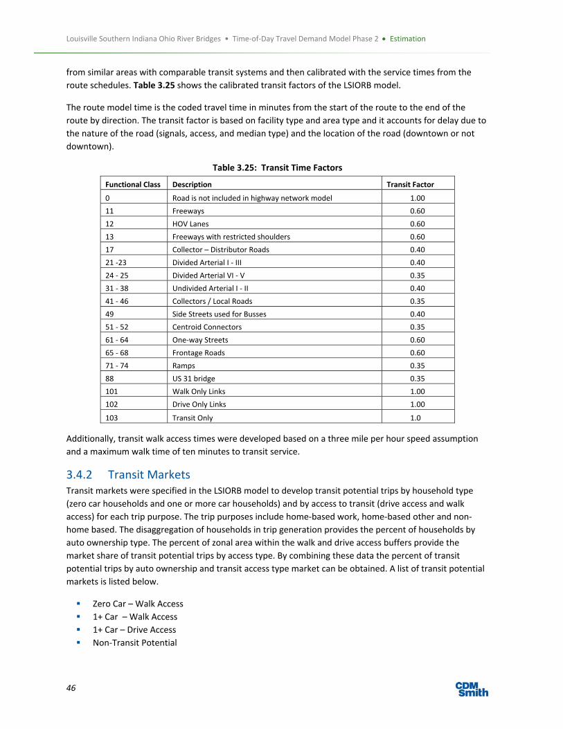
Louisville Southern Indiana Ohio River Bridges • Time‐of‐Day Travel Demand Model Phase 2 Estimation
46
from similar areas with comparable transit systems and then calibrated with the service times from the
route schedules. Table 3.25 shows the calibrated transit factors of the LSIORB model.
The route model time is the coded travel time in minutes from the start of the route to the end of the
route by direction. The transit factor is based on facility type and area type and it accounts for delay due to
the nature of the road (signals, access, and median type) and the location of the road (downtown or not
downtown).
Table 3.25: Transit Time Factors
Functional Class Description Transit Factor
0 Road is not included in highway network model 1.00
11 Freeways 0.60
12 HOV Lanes 0.60
13 Freeways with restricted shoulders 0.60
17 Collector – Distributor Roads 0.40
21 ‐23 Divided Arterial I ‐ III 0.40
24 ‐ 25 Divided Arterial VI ‐ V 0.35
31 ‐ 38 Undivided Arterial I ‐ II 0.40
41 ‐ 46 Collectors / Local Roads 0.35
49 Side Streets used for Busses 0.40
51 ‐ 52 Centroid Connectors 0.35
61 ‐ 64 One‐way Streets 0.60
65 ‐ 68 Frontage Roads 0.60
71 ‐ 74 Ramps 0.35
88 US 31 bridge 0.35
101 Walk Only Links 1.00
102 Drive Only Links 1.00
103 Transit Only 1.0
Additionally, transit walk access times were developed based on a three mile per hour speed assumption
and a maximum walk time of ten minutes to transit service.
3.4.2 Transit Markets Transit markets were specified in the LSIORB model to develop transit potential trips by household type
(zero car households and one or more car households) and by access to transit (drive access and walk
access) for each trip purpose. The trip purposes include home‐based work, home‐based other and non‐
home based. The disaggregation of households in trip generation provides the percent of households by
auto ownership type. The percent of zonal area within the walk and drive access buffers provide the
market share of transit potential trips by access type. By combining these data the percent of transit
potential trips by auto ownership and transit access type market can be obtained. A list of transit potential
markets is listed below.
Zero Car – Walk Access
1+ Car – Walk Access
1+ Car – Drive Access
Non‐Transit Potential

Louisville Southern Indiana Ohio River Bridges • Time‐of‐Day Travel Demand Model Phase 2 Estimation
47
3.4.3 Transit Skimming Transit paths and impedance skims are created for each combination of transit mode, access type, and
time of day. The transit modes include local and premium transit; the access types include walk and drive
access to transit; and the time of day periods include peak and mid‐day periods. The peak period skims are
used for the home‐based work trip purpose in the mode choice models and the mid‐day skims are used for
the home‐based other and non‐home based trip purposes in the mode choice models. The transit skims
created in the LSIORB model include:
Peak period, Walk access, Local transit
Peak period, Drive access, Local transit
Peak period, Walk access, Premium transit
Peak period, Drive access, Premium transit
Mid‐day period, Walk access, Local transit
Mid‐day period, Drive access, Local transit
Mid‐day period, Walk access, Premium transit
Mid‐day period, Drive access, Premium transit
The transit paths are skimmed based on the impedances of generalized, fare and transfer cost (regular cost
and peak period discount), travel time, number of transfers, distance (in‐vehicle and drive access), and CBD
flag. Such travel times include in‐vehicle and out of vehicle travel time where the out of vehicle travel time
includes transit walking and driving access time, wait time for initial boardings and transfers, and transfer
time. Toll costs are included in the generalized travel time based on values of time by vehicle occupancy.
Fare costs are included with transfer and drive access operating costs. There is a 25% reduction in fare
costs for work trips due to the number of discounted “frequent user” fares.
3.4.4 Mode Choice Model Mode choice nest logit models (NLMs) were developed based on trip purpose and major transit markets to
determine the share of trips by mode. The top level nest consists of private vehicle, public transit, and non‐
motorized modes that compete with each other. Within each of those major modes more detailed modes
compete at the next level nest. Express bus services run parallel to and, to some extent, compete with local
bus services. Therefore, there is a choice offered between lower cost, slower local service and higher cost,
faster premium service. On the private vehicle side there is also a need to estimate private vehicle
occupancy and how it might change in response to the implementation of toll charges by vehicle
occupancy. The nesting structures of the NLMs for transit potential trips as well as non‐transit potential
trips are shown in Figure 3.18. These NLM nesting structures are applied by trip purpose and by the
following markets.
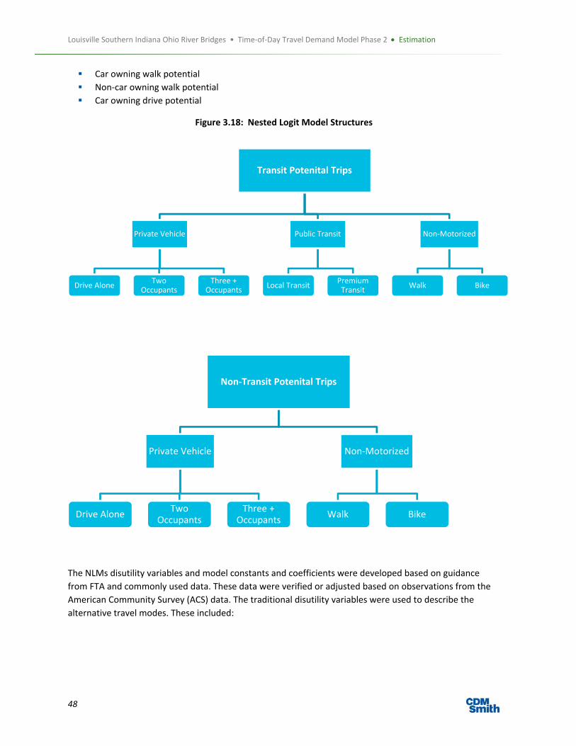
Louisville Southern Indiana Ohio River Bridges • Time‐of‐Day Travel Demand Model Phase 2 Estimation
48
Car owning walk potential
Non‐car owning walk potential
Car owning drive potential
Figure 3.18: Nested Logit Model Structures
The NLMs disutility variables and model constants and coefficients were developed based on guidance
from FTA and commonly used data. These data were verified or adjusted based on observations from the
American Community Survey (ACS) data. The traditional disutility variables were used to describe the
alternative travel modes. These included:
Transit Potenital Trips
Private Vehicle
Drive AloneTwo
OccupantsThree +
Occupants
Public Transit
Local TransitPremium Transit
Non‐Motorized
Walk Bike
Non‐Transit Potenital Trips
Private Vehicle
Drive AloneTwo
OccupantsThree +
Occupants
Non‐Motorized
Walk Bike

Louisville Southern Indiana Ohio River Bridges • Time‐of‐Day Travel Demand Model Phase 2 Estimation
49
In‐vehicle travel time
Out‐vehicle time (waiting for initial boarding as well as transfers and walking/driving access)
Out of pocket costs (on a person trip basis including toll, parking, fare and operating cost for those
driving to transit)
Number of Transfers
CBD or employment density dummy variable
Modal bias constants
These variables are the most sensitive in determining mode shares. As expected time (in‐vehicle, wait,
transfer, and access times), cost (toll, fare, parking and operational costs), and the number of transfers
have a negative effect on the utility equation and the CBD or employment density dummy variable has a
positive effect. Peak travel times and costs are used for home based work trips. Mid‐day times and costs
are used for home based other and non‐home based trips. Table 3.26 shows the disutility variables and
corresponding skimmed model data by mode used for each trip purpose.
Table 3.26: Transit Disutility Variables
Variable
Mode IVTT OVTT COST Transfers CBD
Private Vehicle
Drive Time
Terminal Time Parking Cost (currently inactive), Generalized Cost for Peak (HBW) and Mid‐day (HBO, NHB) based on vehicle occupancy 1, 2, 3
N/A Flag for CBD zone
Transit Transit Time
Wait, Transfer, Access, and Egress Time
Auto Operating Cost * Distance + Fare Cost. Operating cost is only applied for the drive access. Fare cost is discounted by 25% for HBW.
Number of Transfers
Flag for CBD zone
Non‐Motorized
Walk Time
Terminal Time N/A N/A Flag for CBD zone
FTA suggests a set of reasonableness guidelines that should be followed in mode choice model structure
and constant/coefficient estimation. These may be summarized as follows:
Unusual In‐Vehicle Travel Time (IVTT) coefficients – guidance suggests that without compelling evidence
to the contrary IVTT (in minutes) coefficients should be in the range ‐0.03 to ‐0.02. The LSIORB model IVTT
coefficient is ‐0.025.
Mode specific IVTT coefficients – guidance suggests that without compelling evidence to the contrary
mode specific IVTT coefficients should not be used. In the LSIORB model the IVTT coefficient is the same for
all modes.
Unusual ratios of in‐vehicle travel time to Out‐Vehicle Travel Time (OVTT) (walking, waiting, access)
coefficients – guidance suggests that without compelling evidence to the contrary the OVTT/IVTT
coefficient ratio should be in the range 2.0 to 3.0. The OVTT/IVTT coefficient ratio in the LSIORB model is
2.52.
Wide Variation in LogSum coefficients – guidance suggests that without compelling evidence to the
contrary LogSum coefficients should be in the range 0.7 to 1.0. The LSIORB model LogSum coefficients are
in the range of 0.7.
Wide variation of mode choice value of time – guidance suggests that without compelling evidence to the
contrary model implied value of time should be in the range average income /4 to average income / 3. The

Louisville Southern Indiana Ohio River Bridges • Time‐of‐Day Travel Demand Model Phase 2 Estimation
50
LSIORB model uses standard values provided by FTA guidance and recently preformed traffic and revenue
studies of the region.
Non‐logit decision rules – examples are no trip shorter than 3 minutes, no trips with auto access greater
than transit in vehicle time. Guidance is to avoid these types of model structure. Accept some degree of
model inaccuracy instead of over‐defined model structure.
Bizarre Alternative Specific Constants – Guidance is that bias constants should be explainable. A simplified
model structure is often desirable to a very complicated structure for which accurate observed data is not
available.
The resulting LSIORB mode choice model coefficients and constants are presented in Table 3.27. The mode
constants are reported in Table 3.28 are reported by purpose and market.
Table 3.27: Nested Logit Model Parameter Values
Parameters Value
Parameter Coefficients
IVTT ‐0.0250
OVTT ‐0.0630
TRANSFER ‐0.2500
CBD 0.2500
COST (work) ‐0.0023
COST (other) ‐0.0012
Walk Time ‐0.0250
LogSum Coefficents 0.7000
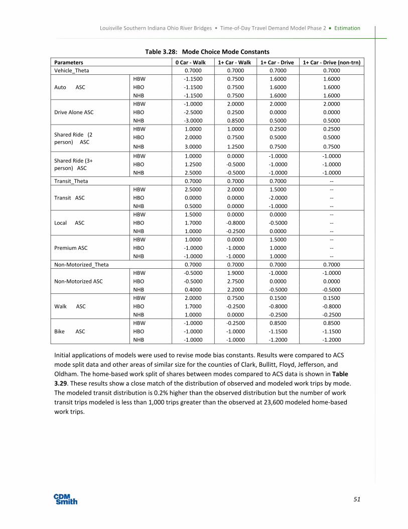
Louisville Southern Indiana Ohio River Bridges • Time‐of‐Day Travel Demand Model Phase 2 Estimation
51
Table 3.28: Mode Choice Mode Constants
Parameters 0 Car ‐ Walk 1+ Car ‐ Walk 1+ Car ‐ Drive 1+ Car ‐ Drive (non‐trn)
Vehicle_Theta 0.7000 0.7000 0.7000 0.7000
Auto ASC
HBW ‐1.1500 0.7500 1.6000 1.6000
HBO ‐1.1500 0.7500 1.6000 1.6000
NHB ‐1.1500 0.7500 1.6000 1.6000
Drive Alone ASC
HBW ‐1.0000 2.0000 2.0000 2.0000
HBO ‐2.5000 0.2500 0.0000 0.0000
NHB ‐3.0000 0.8500 0.5000 0.5000
Shared Ride (2 person) ASC
HBW 1.0000 1.0000 0.2500 0.2500
HBO 2.0000 0.7500 0.5000 0.5000
NHB 3.0000 1.2500 0.7500 0.7500
Shared Ride (3+ person) ASC
HBW 1.0000 0.0000 ‐1.0000 ‐1.0000
HBO 1.2500 ‐0.5000 ‐1.0000 ‐1.0000
NHB 2.5000 ‐0.5000 ‐1.0000 ‐1.0000
Transit_Theta 0.7000 0.7000 0.7000 ‐‐
Transit ASC
HBW 2.5000 2.0000 1.5000 ‐‐
HBO 0.0000 0.0000 ‐2.0000 ‐‐
NHB 0.5000 0.0000 ‐1.0000 ‐‐
Local ASC
HBW 1.5000 0.0000 0.0000 ‐‐
HBO 1.7000 ‐0.8000 ‐0.5000 ‐‐
NHB 1.0000 ‐0.2500 0.0000 ‐‐
Premium ASC
HBW 1.0000 0.0000 1.5000 ‐‐
HBO ‐1.0000 ‐1.0000 1.0000 ‐‐
NHB ‐1.0000 ‐1.0000 1.0000 ‐‐
Non‐Motorized_Theta 0.7000 0.7000 0.7000 0.7000
Non‐Motorized ASC
HBW ‐0.5000 1.9000 ‐1.0000 ‐1.0000
HBO ‐0.5000 2.7500 0.0000 0.0000
NHB 0.4000 2.2000 ‐0.5000 ‐0.5000
Walk ASC
HBW 2.0000 0.7500 0.1500 0.1500
HBO 1.7000 ‐0.2500 ‐0.8000 ‐0.8000
NHB 1.0000 0.0000 ‐0.2500 ‐0.2500
Bike ASC
HBW ‐1.0000 ‐0.2500 0.8500 0.8500
HBO ‐1.0000 ‐1.0000 ‐1.1500 ‐1.1500
NHB ‐1.0000 ‐1.0000 ‐1.2000 ‐1.2000
Initial applications of models were used to revise mode bias constants. Results were compared to ACS
mode split data and other areas of similar size for the counties of Clark, Bullitt, Floyd, Jefferson, and
Oldham. The home‐based work split of shares between modes compared to ACS data is shown in Table
3.29. These results show a close match of the distribution of observed and modeled work trips by mode.
The modeled transit distribution is 0.2% higher than the observed distribution but the number of work
transit trips modeled is less than 1,000 trips greater than the observed at 23,600 modeled home‐based
work trips.

Louisville Southern Indiana Ohio River Bridges • Time‐of‐Day Travel Demand Model Phase 2 Estimation
52
Table 3.29: Mode Split Trip Distribution
ACS 3 Year Data (2006 – 2008)
Observed Distribution Modeled Distribution
Total: 100.0% 100.0%
Drove alone 84.5% 81.0%
In 2‐person carpool 7.9% 9.4%
In 3+‐person carpool 1.9% 2.0%
Public transportation 3.2% 4.3%
Walked 2.3% 2.7%
Bicycle 0.3% 0.7%
The split of transit shares by trip purpose compared to the observed survey data from the Charleston Area
Transportation Study is shown in Table 3.30.
Table 3.30: Transit Trip Distribution by Trip Purpose
Trip Purpose LSIORB Distribution CHATS Distribution
HBW 60.1% 56.4%
HBO 32.1% 32.4%
NHB 7.9% 11.1%
Total Trips 100% 100%
The mode choice model was borrowed from an area of similar size and transit usage. It was recently
estimated with new survey data so was felt was suitable for application to this region. The model that was
used did have a different implied value of time. As part of model application, the value of time was
changed to be consistent with the value used in other parts of the model. Results of the analysis showed
no change in the mode share under base year or forecast conditions.
3.5 External Model The LSIORB TOD Model has an external sub‐model that includes the following components:
External – Internal
– Auto
– Truck
External – External
– Auto
– Truck
The first step in the application of the external sub‐model is the development auto and truck volumes at
the cordon line. The 2007 data is reported in Table 3.31 and includes the distribution of the auto and truck
into the EI and EE components. The distribution is based on the findings from the external OD survey
discussed in section 3.5.1.
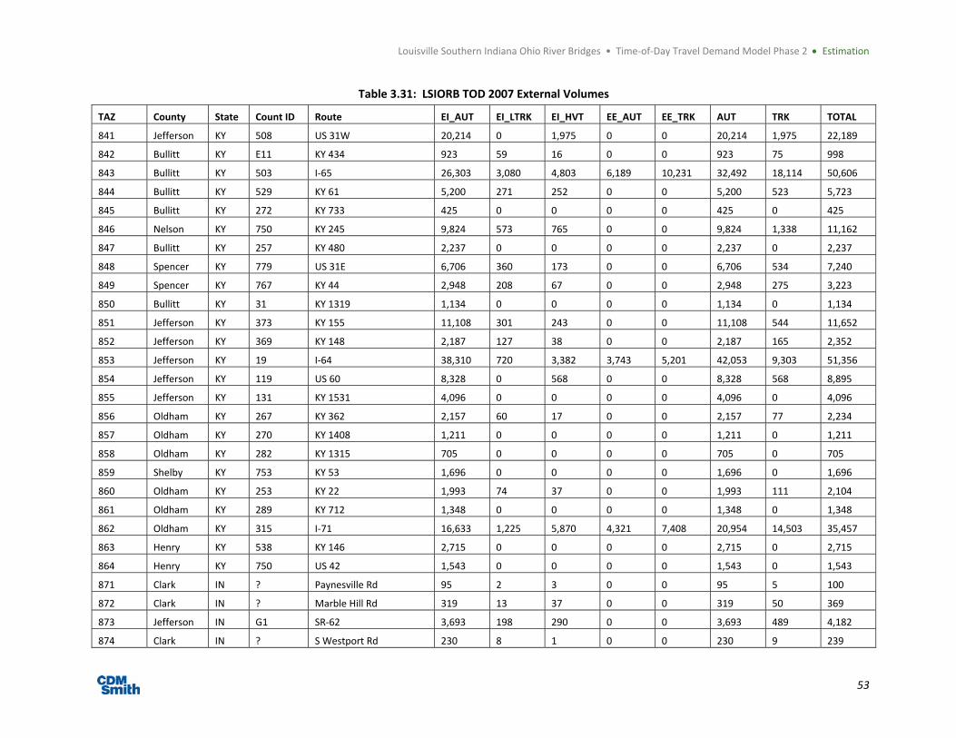
Louisville Southern Indiana Ohio River Bridges • Time‐of‐Day Travel Demand Model Phase 2 Estimation
53
Table 3.31: LSIORB TOD 2007 External Volumes
TAZ County State Count ID Route EI_AUT EI_LTRK EI_HVT EE_AUT EE_TRK AUT TRK TOTAL
841 Jefferson KY 508 US 31W 20,214 0 1,975 0 0 20,214 1,975 22,189
842 Bullitt KY E11 KY 434 923 59 16 0 0 923 75 998
843 Bullitt KY 503 I‐65 26,303 3,080 4,803 6,189 10,231 32,492 18,114 50,606
844 Bullitt KY 529 KY 61 5,200 271 252 0 0 5,200 523 5,723
845 Bullitt KY 272 KY 733 425 0 0 0 0 425 0 425
846 Nelson KY 750 KY 245 9,824 573 765 0 0 9,824 1,338 11,162
847 Bullitt KY 257 KY 480 2,237 0 0 0 0 2,237 0 2,237
848 Spencer KY 779 US 31E 6,706 360 173 0 0 6,706 534 7,240
849 Spencer KY 767 KY 44 2,948 208 67 0 0 2,948 275 3,223
850 Bullitt KY 31 KY 1319 1,134 0 0 0 0 1,134 0 1,134
851 Jefferson KY 373 KY 155 11,108 301 243 0 0 11,108 544 11,652
852 Jefferson KY 369 KY 148 2,187 127 38 0 0 2,187 165 2,352
853 Jefferson KY 19 I‐64 38,310 720 3,382 3,743 5,201 42,053 9,303 51,356
854 Jefferson KY 119 US 60 8,328 0 568 0 0 8,328 568 8,895
855 Jefferson KY 131 KY 1531 4,096 0 0 0 0 4,096 0 4,096
856 Oldham KY 267 KY 362 2,157 60 17 0 0 2,157 77 2,234
857 Oldham KY 270 KY 1408 1,211 0 0 0 0 1,211 0 1,211
858 Oldham KY 282 KY 1315 705 0 0 0 0 705 0 705
859 Shelby KY 753 KY 53 1,696 0 0 0 0 1,696 0 1,696
860 Oldham KY 253 KY 22 1,993 74 37 0 0 1,993 111 2,104
861 Oldham KY 289 KY 712 1,348 0 0 0 0 1,348 0 1,348
862 Oldham KY 315 I‐71 16,633 1,225 5,870 4,321 7,408 20,954 14,503 35,457
863 Henry KY 538 KY 146 2,715 0 0 0 0 2,715 0 2,715
864 Henry KY 750 US 42 1,543 0 0 0 0 1,543 0 1,543
871 Clark IN ? Paynesville Rd 95 2 3 0 0 95 5 100
872 Clark IN ? Marble Hill Rd 319 13 37 0 0 319 50 369
873 Jefferson IN G1 SR‐62 3,693 198 290 0 0 3,693 489 4,182
874 Clark IN ? S Westport Rd 230 8 1 0 0 230 9 239

Louisville Southern Indiana Ohio River Bridges • Time‐of‐Day Travel Demand Model Phase 2 Estimation
54
TAZ County State Count ID Route EI_AUT EI_LTRK EI_HVT EE_AUT EE_TRK AUT TRK TOTAL
875 Clark IN 1P SR‐203 876 0 0 0 0 876 0 876
876 Clark IN 3H SR‐3 1,567 33 67 0 0 1,567 100 1,667
877 Clark IN ? S Slate Ford Rd 270 0 0 0 0 270 0 270
878 Clark IN 10F US 31 4,508 125 118 0 0 4,508 242 4,750
879 Clark IN 1B I‐65 14,193 0 8,978 6,518 7,284 20,710 16,262 36,973
880 Clark IN ? S Bloomington Trl Rd 527 13 1 0 0 527 14 541
881 Clark IN 1N SR‐160 1,912 23 12 0 0 1,912 34 1,946
882 Clark IN ? Pixley Knob Rd 134 1 1 0 0 134 1 135
883 Clark IN 1J SR‐60 8,067 181 401 0 0 8,067 582 8,649
884 Floyd IN ? Martinsburg Knob Rd 367 0 0 0 0 367 0 367
885 Floyd IN 2M SR‐335 1,210 15 35 0 0 1,210 50 1,260
886 Floyd IN 1C US 150 6,768 188 316 0 0 6,768 504 7,272
887 Floyd IN ? Bradford Rd 0 0 0 0 0 0 0 0
888 Floyd IN ? Nadorff Rd 0 0 0 0 0 0 0 0
889 Floyd IN 1H SR‐64 7,806 107 179 0 0 7,806 286 8,092
890 Floyd IN ? Old Lanesville Rd 0 0 0 0 0 0 0 0
891 Floyd IN 1A I‐64 18,470 0 5,031 4,214 5,170 22,685 10,201 32,885
892 Floyd IN 1E SR‐62 2,603 34 13 0 0 2,603 48 2,651
893 Floyd IN 1D SR‐11 602 10 5 0 0 602 15 617
894 Floyd IN 1J SR‐111/River Rd 11,362 138 89 0 0 11,362 227 11,589

Louisville Southern Indiana Ohio River Bridges • Time‐of‐Day Travel Demand Model Phase 2 Estimation
55
3.5.1 Through Demand Data Collection This section describes the data and methodology used to develop external‐to‐external through trips for five
major external stations of the LSIORB study area. The external‐to‐external through trips are developed
based on origin‐destination survey data and traffic counts collected by The Traffic Group, Inc. in September
of 2010. For each external station surveyed, traffic counts and license plate counts as well as the plate‐to‐
count ratio are reported for total vehicles, passenger vehicles, and heavy vehicles. This data is shown in the
Table 3.32 and the locations follow in Figure 3.19.
Table 3.32: Observed Traffic Counts and Recorded License Plates
Station
Traffic Count via Sensor Plates Recorded & Used Count / Plates ‐ Expansion
Total Count
Passenger Count
HV Count Total PlatesPassenger Plates
HV PlatesTotal Factor
PC FactorHV Factor
1N I‐65 North 18,317 10,008 8,309 11,934 6,547 5,387 1.535 1.529 1.542
1S 18,445 10,423 8,022 12,526 6,982 5,544 1.473 1.493 1.447
2N I‐71 East
28,167 16,066 12,101 23,288 18,300 4,988 1.210 0.878 2.426
2S 29,095 20,403 8,692 21,867 17,386 4,481 1.331 1.174 1.940
3E I‐64 East
25,730 19,080 6,650 22,124 18,635 3,489 1.163 1.024 1.906
3W 25,309 18,376 6,933 20,338 16,739 3,599 1.244 1.098 1.926
4N I‐65 South 25,582 15,752 9,830 21,646 14,486 7,160 1.182 1.087 1.373
4S 26,081 15,101 10,980 12,246 12,246 6,402 2.130 1.233 1.715
5E I‐64 West
15,920 10,210 5,710 9,823 7,433 2,390 1.621 1.374 2.389
5W 15,826 11,657 4,169 8,680 6,493 2,187 1.823 1.795 1.906
Total 228,472 147,076 81,396 164,472 125,247 45,627 1.389 1.174 1.784

Louisville Southern Indiana Ohio River Bridges • Time‐of‐Day Travel Demand Model Phase 2 Estimation
56
Figure 3.19: Origin Destination Survey Locations
Site 1
Site 2
Site 3
Site 4
Site 5

Louisville Southern Indiana Ohio River Bridges • Time‐of‐Day Travel Demand Model Phase 2 Estimation
57
Results from the license plate recognition and matching survey were adjusted for study area inbound and
outbound movements and factored to match the recorded traffic count data. Expansion factors and the
fratar process are used to adjust the survey license plate data into balanced external through movements
between the five external stations for both passenger vehicles and heavy vehicles. Note that heavy vehicles
include both light and heavy trucks. The below sections describe the procedures for developing external‐
to‐external through trips for passenger and heavy vehicles.
3.5.2 Through Passenger Vehicles Demand The origin‐destination survey conducted by The Traffic Group, Inc. provided data on external trip
movements by direction including external‐to‐external (EE) and external‐to‐internal (EI) movements for
passenger vehicles. This data is shown in the Table 3.33. The license plates were matched for at the first
and last location only throughout the 24‐hour period. Thus, some illogical movements between the
directional external stations are recorded. For example, the southbound trips from external station 1 (1S)
going to southbound station 2 (2S) or to northbound station 4 (4N) is not a direct movement but there are
other external‐to‐internal movements not recorded within these two endpoints that compose this trip
chain. Therefore, these trips are considered EI trips. Similarly, the matrix diagonal highlighted in light
orange are EI trips where a license plate was recorded initially but no match was found. In other words, a
trip entered or exited the study area but did not return.
Table 3.33: Directional External Passenger Vehicle Matched License Plates
1N 1S 2N 2S 3E 3W 4N 4S 5E 5W Total
1N 4,844 778 142 79 151 105 82 110 101 155 6,547
1S 906 3,580 141 59 817 80 67 920 107 305 6,982
2N 176 56 13,278 4,048 124 136 82 147 95 158 18,300
2S 210 61 6,897 8,291 262 103 101 1,005 92 364 17,386
3E 209 60 163 117 13,029 4,605 101 115 85 151 18,635
3W 716 55 268 93 5,980 8,754 67 157 85 564 16,739
4N 1,131 74 1,328 94 225 91 7,806 3,494 81 162 14,486
4S 176 55 226 63 134 72 2,434 8,886 88 112 12,246
5E 369 113 423 76 614 97 70 128 4,009 1,534 7,433
5W 198 66 138 61 130 65 58 76 1,063 4,638 6,493
Total 8,935 4,898 23,004 12,981 21,466 14,108 10,868 15,038 5,806 8,143 125,247
There are a total of 125,247 passenger vehicle trips recorded by the origin‐destination license plate
matching survey. In comparison to Table 3.32, the sum of the rows (productions) match the number of
plates recorded for passenger vehicles. The sum of the columns (attractions) does not match the number
of plates recorded and shows an imbalance of trips. The trip imbalance could be a result of the low plate
matching rate for external station five. Additional details can be seen in the Automatic License Plate
Recognition and Origin & Destination Study report developed by The Traffic Group, Inc.
The directional external passenger vehicle trips were condensed to only the logical external station
movements between the five external stations. Based on the location of the stations, the locations of 1S,
2S, 3W, 4N, and 5E are entry points to the study area and the locations of 1N, 2N, 3E, 4S, and 5W are exit
points to the study area. A matrix table was developed that includes the survey external trips from entry
points to exit points for passenger vehicles. This table is shown in Table 3.34.

Louisville Southern Indiana Ohio River Bridges • Time‐of‐Day Travel Demand Model Phase 2 Estimation
58
Table 3.34: External Passenger Vehicle Matched License Plates
1N 2N 3E 4S 5W Total
1S 906 141 817 920 305 3,089
2S 210 6,897 262 1,005 364 8,738
3W 716 268 5,980 157 564 7,685
4N 1,131 1,328 225 3,494 162 6,340
5E 369 423 614 128 1,534 3,068
Total 3,332 9,057 7,898 5,704 2,929 28,920
The external passenger vehicle trips were further condensed to only the EE trips between the five external
stations and all EI trips were removed. See Table 3.35.
Table 3.35: External to External Passenger Vehicle Matched License Plates
1N 2N 3E 4S 5W Total
1S 0 141 817 920 305 2,183
2S 210 0 262 1,005 364 1,841
3W 716 268 0 157 564 1,705
4N 1,131 1,328 225 0 162 2,846
5E 369 423 614 128 0 1,534
Total 2,426 2,160 1,918 2,210 1,395 10,109
The EE trips were then expanded to match the observed counts using expansion factors. The expansion
factors are shown in Table 3.32 as the count‐to‐plate ratios. Table 3.36 shows the expansion of the EE
productions and attractions. Note that external station 2N has a decreasing expansion rate. The issue of
the decreasing expansion rate for station 2N (attraction) as well as the imbalance of the attraction trip
totals (Table 3.35) to the matched plates (Table 3.33) results in some uncertainty with the attraction trips.
Therefore, due to more confidence in the production data, the expanded external trip productions are
used to fratar the survey EE passenger trips to the expanded EE trips to be used in the LSIORB travel
demand model.
Table 3.36: Expanded Passenger Vehicle External to External Trip Productions and Attractions
Productions Attractions
Survey EE Trips
Expansion Factor
Expanded Productions
Survey EE Trips
Expansion Factor
Expanded Attractions
1S 2,183 1.473 3,259 1N 2,426 1.529 3,708
2S 1,841 1.174 2,160 2N 2,160 0.878 1,896
3W 1,705 1.098 1,872 3E 1,918 1.024 1,964
4N 2,846 1.087 3,095 4S 2,210 1.233 2,725
5E 1,534 1.374 2,107 5W 1,395 1.795 2,504
Total 10,109 n/a 12,493 Total 10,109 n/a 12,798
The TransCAD modeling software was used to fratar the raw survey data of EE trips (Table 3.35) with the
sum of the expanded EE productions (Table 3.36) for passenger vehicles. The result of the fratar procedure
is a daily external‐to‐external trip matrix. As shown in Table 3.37 there are approximately 12,500 external
through trips for passenger vehicles in the LSIORB study area.
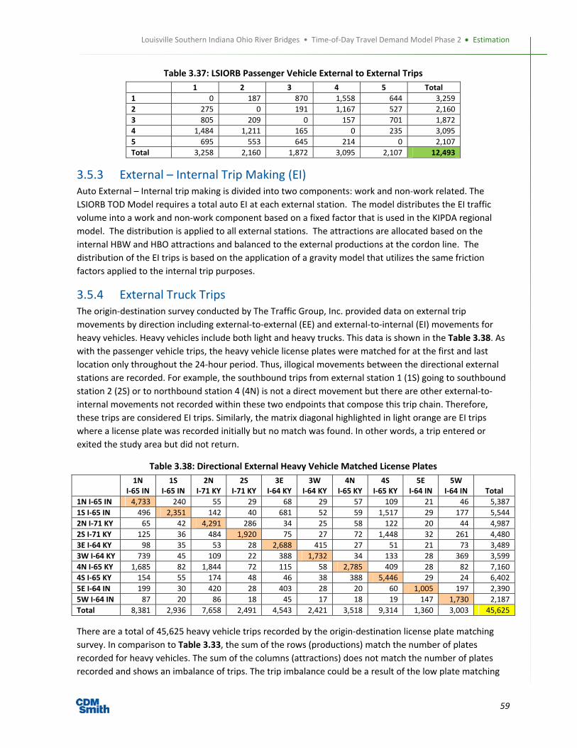
Louisville Southern Indiana Ohio River Bridges • Time‐of‐Day Travel Demand Model Phase 2 Estimation
59
Table 3.37: LSIORB Passenger Vehicle External to External Trips
1 2 3 4 5 Total
1 0 187 870 1,558 644 3,259
2 275 0 191 1,167 527 2,160
3 805 209 0 157 701 1,872
4 1,484 1,211 165 0 235 3,095
5 695 553 645 214 0 2,107
Total 3,258 2,160 1,872 3,095 2,107 12,493
3.5.3 External – Internal Trip Making (EI) Auto External – Internal trip making is divided into two components: work and non‐work related. The
LSIORB TOD Model requires a total auto EI at each external station. The model distributes the EI traffic
volume into a work and non‐work component based on a fixed factor that is used in the KIPDA regional
model. The distribution is applied to all external stations. The attractions are allocated based on the
internal HBW and HBO attractions and balanced to the external productions at the cordon line. The
distribution of the EI trips is based on the application of a gravity model that utilizes the same friction
factors applied to the internal trip purposes.
3.5.4 External Truck Trips The origin‐destination survey conducted by The Traffic Group, Inc. provided data on external trip
movements by direction including external‐to‐external (EE) and external‐to‐internal (EI) movements for
heavy vehicles. Heavy vehicles include both light and heavy trucks. This data is shown in the Table 3.38. As
with the passenger vehicle trips, the heavy vehicle license plates were matched for at the first and last
location only throughout the 24‐hour period. Thus, illogical movements between the directional external
stations are recorded. For example, the southbound trips from external station 1 (1S) going to southbound
station 2 (2S) or to northbound station 4 (4N) is not a direct movement but there are other external‐to‐
internal movements not recorded within these two endpoints that compose this trip chain. Therefore,
these trips are considered EI trips. Similarly, the matrix diagonal highlighted in light orange are EI trips
where a license plate was recorded initially but no match was found. In other words, a trip entered or
exited the study area but did not return.
Table 3.38: Directional External Heavy Vehicle Matched License Plates
1N I‐65 IN
1S I‐65 IN
2N I‐71 KY
2S I‐71 KY
3E I‐64 KY
3W I‐64 KY
4N I‐65 KY
4S I‐65 KY
5E I‐64 IN
5W I‐64 IN Total
1N I‐65 IN 4,733 240 55 29 68 29 57 109 21 46 5,387
1S I‐65 IN 496 2,351 142 40 681 52 59 1,517 29 177 5,544
2N I‐71 KY 65 42 4,291 286 34 25 58 122 20 44 4,987
2S I‐71 KY 125 36 484 1,920 75 27 72 1,448 32 261 4,480
3E I‐64 KY 98 35 53 28 2,688 415 27 51 21 73 3,489
3W I‐64 KY 739 45 109 22 388 1,732 34 133 28 369 3,599
4N I‐65 KY 1,685 82 1,844 72 115 58 2,785 409 28 82 7,160
4S I‐65 KY 154 55 174 48 46 38 388 5,446 29 24 6,402
5E I‐64 IN 199 30 420 28 403 28 20 60 1,005 197 2,390
5W I‐64 IN 87 20 86 18 45 17 18 19 147 1,730 2,187
Total 8,381 2,936 7,658 2,491 4,543 2,421 3,518 9,314 1,360 3,003 45,625
There are a total of 45,625 heavy vehicle trips recorded by the origin‐destination license plate matching
survey. In comparison to Table 3.33, the sum of the rows (productions) match the number of plates
recorded for heavy vehicles. The sum of the columns (attractions) does not match the number of plates
recorded and shows an imbalance of trips. The trip imbalance could be a result of the low plate matching

Louisville Southern Indiana Ohio River Bridges • Time‐of‐Day Travel Demand Model Phase 2 Estimation
60
rate for external station five. Additional details can be seen in the Automatic License Plate Recognition and
Origin & Destination Study report developed by The Traffic Group, Inc.
The directional external heavy vehicle trips were condensed to only the logical external station movements
between the five external stations. Based on the location of the stations, the locations of 1S, 2S, 3W, 4N, and 5E
are entry points to the study area and the locations of 1N, 2N, 3E, 4S, and 5W are exit points to the study area. A
matrix table was developed that includes the survey external trips from entry points to exit points for heavy
vehicles. This table is shown in Table 3.39.
Table 3.39: External Heavy Vehicle Matched License Plates
1N 2N 3E 4S 5W Total
1S 496 142 681 1,517 177 3,013
2S 125 484 75 1,448 261 2,393
3W 739 109 388 133 369 1,738
4N 1,685 1,844 115 409 82 4,135
5E 199 420 403 60 197 1,279
Total 3,244 2,999 1,662 3,567 1,086 12,558
The external heavy vehicle trips were further condensed to only the EE trips between the five external
stations and all EI trips were removed. See Table 3.40.
Table 3.40: External to External Heavy Vehicle Matched License Plates
1N 2N 3E 4S 5W Total
1S 0 142 681 1,517 177 2,517
2S 125 0 75 1,448 261 1,909
3W 739 109 0 133 369 1,350
4N 1,685 1,844 115 0 82 3,726
5E 199 420 403 60 0 1,082
Total 2,748 2,515 1,274 3,158 889 10,584
The EE trips were then expanded to match the observed counts using expansion factors. The expansion
factors are shown in Table 3.33 as the count‐to‐plate ratios. Table 3.41 shows the expansion of the EE
productions and attractions. Similar to the issues with the heavy vehicle trip attractions and due to more
confidence in the production data, the expanded external trip productions are used to fratar the survey EE
heavy trips to the expanded EE trips to be used in the LSIORB travel demand model.
Table 3.41: Expanded Heavy Vehicle External to External Trip Productions and Attractions
Productions Attractions
Survey EE Trips
Expansion Factor
Expanded Productions
Survey EE Trips
Expansion Factor
Expanded Attractions
1S 2,517 1.447 3,642 1N 2,748 1.542 4,239
2S 1,909 1.940 3,704 2N 2,515 2.426 6,103
3W 1,350 1.926 2,601 3E 1,274 1.906 2,428
4N 3,726 1.373 5,115 4S 3,158 1.715 5,416
5E 1,082 2.389 2,585 5W 889 1.906 1,695
Total 10,584 n/a 17,647 Total 10,584 n/a 19,880
The TransCAD modeling software was used to fratar the raw survey data of EE trips (Table 9) with the sum
of the expanded EE productions (Table 10) for heavy vehicles. The result of the fratar procedure is a daily
external‐to‐external trip matrix. As shown in Table 3.42 there are approximately 17,600 external through
trips for heavy vehicles in the LSIORB study area.

Louisville Southern Indiana Ohio River Bridges • Time‐of‐Day Travel Demand Model Phase 2 Estimation
61
Table 3.42: LSIORB Heavy Vehicle External to External Trips
1 2 3 4 5 Total
1 0 148 1,028 2,071 395 3,642
2 158 0 150 2,623 773 3,704
3 1,003 162 0 259 1,176 2,601
4 2,111 2,535 229 0 241 5,115
5 371 860 1,193 161 0 2,585
Total 3,643 3,705 2,601 5,113 2,585 17,647
3.6 Truck Model The previous section discussed the development of the external‐external truck movements. The LSIORB
TOD Model includes the movement of trucks that are internal to the region and External‐Internal which we
are calling the truck model. The development of the Sub‐Model included the following steps:
Development of seed truck trip table
Matrix adjustment using ODME
For the LSIORB TOD Truck Model, all trucks are combined into one vehicle type. The trucks modeled
include multi unit vehicles, or heavy trucks, and single unit vehicles with more than 4 tires. The truck
model does not include the movement of commercial vehicles which are represented in the model as part
of the NHB trip purpose.
3.6.1 Seed Truck Trip Table The first step in the development of the Internal and External‐Internal Truck trip tables was the
development of a seed trip table for 2007.
3.6.1.1 Internal Truck Movements
The zonal generation of the single unit, and multi unit truck trips is estimated using regression models that
input the zonal demographics and calibrated parameters. The productions and attractions use the same
model coefficients.
The current state of the practice for truck models is to use the Quick Response Freight Manual II, FHWA
(2007) for trip generation. These coefficients were originally calibrated from data collected in Phoenix,
Arizona in the 1990s. The QRFM coefficients are shown in Figure 3.20.
Figure 3.20: Quick Response Freight Manual ‐ Generation Rates (Source: QRFM, Table 4.1)
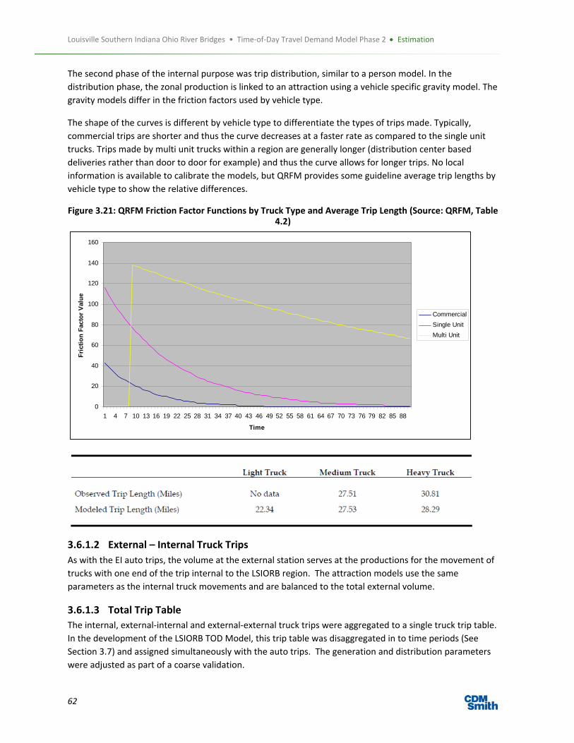
Louisville Southern Indiana Ohio River Bridges • Time‐of‐Day Travel Demand Model Phase 2 Estimation
62
The second phase of the internal purpose was trip distribution, similar to a person model. In the
distribution phase, the zonal production is linked to an attraction using a vehicle specific gravity model. The
gravity models differ in the friction factors used by vehicle type.
The shape of the curves is different by vehicle type to differentiate the types of trips made. Typically,
commercial trips are shorter and thus the curve decreases at a faster rate as compared to the single unit
trucks. Trips made by multi unit trucks within a region are generally longer (distribution center based
deliveries rather than door to door for example) and thus the curve allows for longer trips. No local
information is available to calibrate the models, but QRFM provides some guideline average trip lengths by
vehicle type to show the relative differences.
Figure 3.21: QRFM Friction Factor Functions by Truck Type and Average Trip Length (Source: QRFM, Table 4.2)
3.6.1.2 External – Internal Truck Trips
As with the EI auto trips, the volume at the external station serves at the productions for the movement of
trucks with one end of the trip internal to the LSIORB region. The attraction models use the same
parameters as the internal truck movements and are balanced to the total external volume.
3.6.1.3 Total Trip Table
The internal, external‐internal and external‐external truck trips were aggregated to a single truck trip table.
In the development of the LSIORB TOD Model, this trip table was disaggregated in to time periods (See
Section 3.7) and assigned simultaneously with the auto trips. The generation and distribution parameters
were adjusted as part of a coarse validation.
0
20
40
60
80
100
120
140
160
1 4 7 10 13 16 19 22 25 28 31 34 37 40 43 46 49 52 55 58 61 64 67 70 73 76 79 82 85 88
Time
Fri
ctio
n F
acto
r V
alu
e
Commercial
Single Unit
Multi Unit

Louisville Southern Indiana Ohio River Bridges • Time‐of‐Day Travel Demand Model Phase 2 Estimation
63
3.6.2 Matrix Adjustment Based on the modeled truck trip table developed for 2007, an ODME process was completed to create a
more accurate truck trip table for assignment in the model. In total, over 550 truck counts were identified
as part of the count database created in Phase I. Because of inconsistency in the reporting of truck data
between Indiana and Kentucky, it was only possible to develop a combined truck count rather than
distinguish between single unit and multi unit vehicles (Figure 3.22).
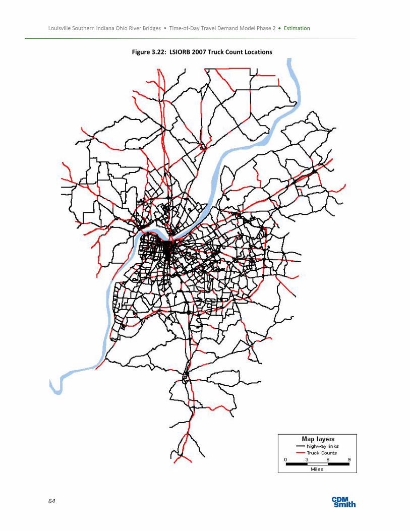
Louisville Southern Indiana Ohio River Bridges • Time‐of‐Day Travel Demand Model Phase 2 Estimation
64
Figure 3.22: LSIORB 2007 Truck Count Locations

Louisville Southern Indiana Ohio River Bridges • Time‐of‐Day Travel Demand Model Phase 2 Estimation
65
The resulting intra and external‐internal truck trip tables were added to the external through trips and
applied to the ODME process using the identified counts. The external through and external‐internal
productions were held constant allowing the internal end of the EI and internal trips to change.
An assessment was made of the resulting ODME trip table versus the zonal generation results. The
resulting trip table marginals from the ODME and modeled trip table were compared and the resulting r‐
squared was greater than 0.8. (Figure 3.23)
Figure 3.23: ODME vs. Modeled Trip Table Marginals
3.7 Time of Day Model A key feature of the LSIORB TOD Model is the disaggregation of the daily trip tables created by mode
choice into time of day periods for traffic assignment. The benefit to this design is that congestion in the
system is better represented and the impact on route choice. Further, it provides for additional policy
sensitivity in the model.
3.7.1 Period Definition In defining periods for a Time of Day Model, the standard approach is to define a period to be at least one
hour in length. In the case of the LSIORB TOD Model, the periods were defined based on the following
criteria:
Capturing majority of directional commuting trips
Period allowed for all trips to be completed (period longer than longest trip)
Capturing activities of trip purposes
Figure 3.24 shows the distribution of trips by trip purpose. From the graph, the prominence of work trips
being made in the am peak and pm peak periods becomes clear. As well, the high activity of NHB and HBO
activity being made between the peak periods becomes clear.
y = 1.1197xR² = 0.8366
0.00
1000.00
2000.00
3000.00
4000.00
5000.00
6000.00
7000.00
8000.00
9000.00
0.00 2000.00 4000.00 6000.00 8000.00
HTRK
Linear (HTRK)

Louisville Southern Indiana Ohio River Bridges • Time‐of‐Day Travel Demand Model Phase 2 Estimation
66
Figure 3.24: Distribution of Internal Trips by Hour (Source: 2000 KIPDA Household Survey)
Based on a review of the information presented above, the following periods were identified for the
LSIORB TOD Model:
AM Period: 6am to 9am (3 Hours)
Mid – Day: 9am to 3pm (6 Hours)
PM Period: 3pm to 6pm (3 Hours)
Overnight: 6pm to 6am (12 Hours)
Through the development of the LSIORB TOD Model, it was decided that the AM and PM periods would be
further disaggregated to individual hours to fully capture the peak congestion in the system.
Based on these periods, the directionality of the trips were defined using the household travel survey data.
For home based trips, the orientation of trips from home to attraction and attraction to home were
defined. This creates the directional movement of trips observed in reality in the model. Table
3.43provides the distribution by direction by purpose. When reviewing the information, the direction of
travel from home to work (DEP) for HBW appears in the AM Period with very low percentages of trips in
the work to home (RTN) direction. In the PM period, this pattern is reversed as expected.
0.00
0.02
0.04
0.06
0.08
0.10
0.12
0.14
0.16
0 2 4 6 8 10 12 14 16 18 20 22
Percent of Trips Mad
e
Hour
HBW
HBO
NHB

Louisville Southern Indiana Ohio River Bridges • Time‐of‐Day Travel Demand Model Phase 2 Estimation
67
Table 3.43: Directional Trip Purpose Diurnal Factors (Source: 2000 KIPDA Household Survey)
Hour HBW HBO NHB DEP_HBW RTN_HBW DEP_HBO RTN_HBO TOTAL
0 1.07% 0.27% 0.17% 0.16% 0.91% 0.03% 0.24% 0.41%
1 0.43% 0.07% 0.11% 0.04% 0.40% 0.00% 0.07% 0.15%
2 0.34% 0.04% 0.02% 0.11% 0.24% 0.01% 0.03% 0.10%
3 0.25% 0.06% 0.06% 0.18% 0.07% 0.02% 0.04% 0.10%
4 0.62% 0.06% 0.00% 0.54% 0.07% 0.05% 0.01% 0.16%
5 2.37% 0.20% 0.05% 2.14% 0.24% 0.18% 0.01% 0.61%
6 7.19% 1.34% 0.40% 6.78% 0.42% 1.28% 0.06% 2.32%
7 12.36% 6.87% 2.67% 11.85% 0.51% 6.56% 0.30% 6.98%
8 12.74% 8.70% 5.16% 12.25% 0.49% 7.69% 1.01% 8.68%
9 5.07% 5.84% 4.87% 4.66% 0.42% 4.86% 0.98% 5.45%
10 2.77% 5.05% 5.90% 2.17% 0.60% 3.69% 1.37% 4.79%
11 1.96% 4.60% 9.05% 1.23% 0.72% 2.80% 1.79% 5.12%
12 2.07% 5.15% 11.92% 0.80% 1.27% 2.37% 2.78% 6.14%
13 2.81% 5.15% 10.80% 1.56% 1.25% 2.28% 2.87% 6.03%
14 3.55% 6.45% 9.14% 1.81% 1.74% 2.64% 3.81% 6.50%
15 4.71% 10.43% 10.38% 1.32% 3.39% 2.26% 8.16% 9.24%
16 8.70% 8.83% 9.20% 1.49% 7.21% 2.36% 6.47% 8.89%
17 14.69% 7.15% 7.82% 0.98% 13.71% 2.31% 4.84% 8.87%
18 7.03% 7.84% 4.97% 0.54% 6.49% 3.53% 4.32% 6.98%
19 3.06% 5.99% 3.05% 0.56% 2.50% 2.83% 3.16% 4.68%
20 1.54% 4.16% 2.37% 0.25% 1.29% 0.82% 3.33% 3.19%
21 1.38% 3.05% 1.32% 0.27% 1.11% 0.41% 2.65% 2.29%
22 1.78% 1.91% 0.48% 0.65% 1.12% 0.28% 1.62% 1.54%
23 1.52% 0.80% 0.09% 0.56% 0.96% 0.09% 0.71% 0.78%
A similar process was completed for the external auto and truck trips. Based on the counts collected as
part of the video OD survey, a distribution of auto and truck trips entering the region was defined and used
to generate the period factors for external – external auto and truck as well as the external‐internal auto
and truck trips. (Figure 3.25)
Figure 3.25: External Auto and Truck Hourly Distributions
0
0.01
0.02
0.03
0.04
0.05
0.06
0.07
0.08
0.09
1 2 3 4 5 6 7 8 9 101112131415161718192021222324
AUTO
TRUCK

Louisville Southern Indiana Ohio River Bridges • Time‐of‐Day Travel Demand Model Phase 2 Estimation
68
The table and figures above provide the rationale for the period definitions and resulting diurnal factors for
the LSIORB TOD Model. In application, the diurnal factors are applied to the daily vehicle trips that are
output from the mode choice model by mode (SOV, HOV2, and HOV3+) and by purpose. The time of day
disaggregation converts the PA trips to OD format. The time of day model does not include a choice model,
but instead the period distribution and directionality of trips are fixed in the base year and forecast.
3.8 Traffic Assignment The LSIORB Phase II Model uses a multi‐class user equilibrium traffic assignment that relies on a
generalized cost impedance function. As described previously in this memo, the free flow travel time is
specified in the network as is the generalized cost for each link. The generalized cost is the operating cost
per mile plus any tolls added to the network links if included in the scenario. The TransCAD graphical user
interface allows the opportunity to apply unique values of time by income group, and for trucks. Operating
cost is applied by Auto and Truck. Unique toll rates can be applied for Auto by occupancy and for trucks for
peak periods and for mid‐day / overnight.
3.8.1 Assignment Fields Table 3.44 indicates the fields used for each period assignment.
Table 3.44: Assignment Parameters
Field AM (1 – 3) MD PM (1‐3)_ NT
Free Flow Time AB_AFF_Time / BA_AFF_Time
Capacity AB_HR_CAP /
BA_HR_CAP
AB_MD_CAP /
BA_MD_CAP
AB_HR_CAP /
BA_HR_CAP
AB_NT_CAP /
BA_NT_CAP
Alpha ALPHA
Beta BETA
Field Descriptions: AB_AFF_Time / BA_AFF_Time: Adjusted free flow travel time based on speed limit, FHWA free flow adjustment plus
uniform signal delay.
AB_HR_CAP / BA_HR_CAP: Directional hourly capacity.
AB_MD_CAP / BA_MD_CAP: Mid‐Day (6 hour) capacity
AB_NT_CAP/ BA_NT_CAP: Overnight (12 hour) capacity
Alpha and Beta: Volume Delay Function parameters
The LSIORB TOD Model was modified to allow the user to test the sensitivity of tolls only in the assignment
process and not in the feedback through distribution and mode choice. To accommodate this in the
network fields, a second set of generalized cost fields (aGC_*) was added. When tolls are not considered
as part of the scenario, either in distribution and mode choice and assignment, the parameters shown in
Table 3.45 are appropriate.
If tolling is considered in the distribution and mode choice as well as assignment, the parameters in Table
3.46 are read by the model. When tolling is only considered as part of assignment, the model reads the GC
fields for trip distribution and mode choice and aGC for assignment. Finally, when a free scenario, the GC
and aGC fields are equal.
3.8.2 Value of Time and Passenger Car Equivalents The TransCAD MMA Generalized Cost assignment methodology converts the link level travel time to a cost
using the value of time by matrix core. The graphical user interface allows the use of unique values of time
by income group for the auto trips, and unique values of time for light truck and heavy truck flows.

Louisville Southern Indiana Ohio River Bridges • Time‐of‐Day Travel Demand Model Phase 2 Estimation
69
A passenger car equivalent is used for the truck purposes including the LtTRK and HvTRK flows. The default
PCE parameter is 2.0 which is reflective of the relatively flat geography in the Louisville region.
3.8.3 Assignment Convergence Each period assignment is set to have a convergence closure of 0.001 and to be reached by 100 iterations.
Through the validation process, the assignments have been converging before the maximum iteration.
Table 3.45: No Toll Generalized Cost by Trip Purpose
Core Name AM / PM Peak Periods MD / NT Periods
HBW1_DA (6‐9) GC_pkDA GC_mdDA
HBW1_SR2 (6‐9) GC_pkSR2 GC_mdSR2
HBW1_SR3 (6‐9) GC_pkSR3 GC_mdSR3
HBW2_DA (6‐9) GC_pkDA GC_mdDA
HBW2_SR2 (6‐9) GC_pkSR2 GC_mdSR2
HBW2_SR3 (6‐9) GC_pkSR3 GC_mdSR3
HBW3_DA (6‐9) GC_pkDA GC_mdDA
HBW3_SR2 (6‐9) GC_pkSR2 GC_mdSR2
HBW3_SR3 (6‐9) GC_pkSR3 GC_mdSR3
EIIEW (6‐9) GC_pkDA GC_mdDA
EIIEO (6‐9) GC_pkDA GC_mdDA
LtTRK (6‐9) GC_LtTRK GC_LtTRK
HvTRK (6‐9) GC_HvTRK GC_HvTRK
EI_LtTRK (6‐9) GC_LtTRK GC_LtTRK
EI_HvTRK (6‐9) GC_HvTRK GC_HvTRK
HBO1_DA (6‐9) GC_pkDA GC_mdDA
HBO1_SR2 (6‐9) GC_pkSR2 GC_mdSR2
HBO1_SR3 (6‐9) GC_pkSR3 GC_mdSR3
HBO2_DA (6‐9) GC_pkDA GC_mdDA
HBO2_SR2 (6‐9) GC_pkSR2 GC_mdSR2
HBO2_SR3 (6‐9) GC_pkSR3 GC_mdSR3
HBO3_DA (6‐9) GC_pkDA GC_mdDA
HBO3_SR2 (6‐9) GC_pkSR2 GC_mdSR2
HBO3_SR3 (6‐9) GC_pkSR3 GC_mdSR3
NHB1_DA (6‐9) GC_pkDA GC_mdDA
NHB1_SR2 (6‐9) GC_pkSR2 GC_mdSR2
NHB1_SR3 (6‐9) GC_pkSR3 GC_mdSR3
NHB2_DA (6‐9) GC_pkDA GC_mdDA
NHB2_SR2 (6‐9) GC_pkSR2 GC_mdSR2
NHB2_SR3 (6‐9) GC_pkSR3 GC_mdSR3
NHB3_DA (6‐9) GC_pkDA GC_mdDA
NHB3_SR2 (6‐9) GC_pkSR2 GC_mdSR2
NHB3_SR3 (6‐9) GC_pkSR3 GC_mdSR3
Auto EE GC_pkDA GC_mdDA
Truck EE GC_HvTRK GC_HvTRK
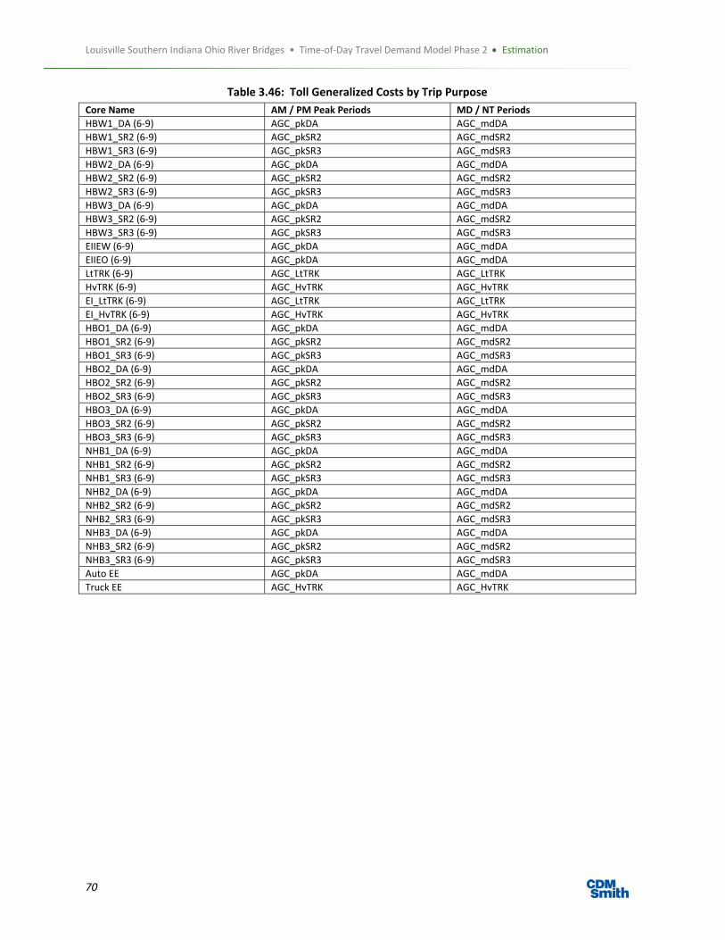
Louisville Southern Indiana Ohio River Bridges • Time‐of‐Day Travel Demand Model Phase 2 Estimation
70
Table 3.46: Toll Generalized Costs by Trip Purpose
Core Name AM / PM Peak Periods MD / NT Periods
HBW1_DA (6‐9) AGC_pkDA AGC_mdDA
HBW1_SR2 (6‐9) AGC_pkSR2 AGC_mdSR2
HBW1_SR3 (6‐9) AGC_pkSR3 AGC_mdSR3
HBW2_DA (6‐9) AGC_pkDA AGC_mdDA
HBW2_SR2 (6‐9) AGC_pkSR2 AGC_mdSR2
HBW2_SR3 (6‐9) AGC_pkSR3 AGC_mdSR3
HBW3_DA (6‐9) AGC_pkDA AGC_mdDA
HBW3_SR2 (6‐9) AGC_pkSR2 AGC_mdSR2
HBW3_SR3 (6‐9) AGC_pkSR3 AGC_mdSR3
EIIEW (6‐9) AGC_pkDA AGC_mdDA
EIIEO (6‐9) AGC_pkDA AGC_mdDA
LtTRK (6‐9) AGC_LtTRK AGC_LtTRK
HvTRK (6‐9) AGC_HvTRK AGC_HvTRK
EI_LtTRK (6‐9) AGC_LtTRK AGC_LtTRK
EI_HvTRK (6‐9) AGC_HvTRK AGC_HvTRK
HBO1_DA (6‐9) AGC_pkDA AGC_mdDA
HBO1_SR2 (6‐9) AGC_pkSR2 AGC_mdSR2
HBO1_SR3 (6‐9) AGC_pkSR3 AGC_mdSR3
HBO2_DA (6‐9) AGC_pkDA AGC_mdDA
HBO2_SR2 (6‐9) AGC_pkSR2 AGC_mdSR2
HBO2_SR3 (6‐9) AGC_pkSR3 AGC_mdSR3
HBO3_DA (6‐9) AGC_pkDA AGC_mdDA
HBO3_SR2 (6‐9) AGC_pkSR2 AGC_mdSR2
HBO3_SR3 (6‐9) AGC_pkSR3 AGC_mdSR3
NHB1_DA (6‐9) AGC_pkDA AGC_mdDA
NHB1_SR2 (6‐9) AGC_pkSR2 AGC_mdSR2
NHB1_SR3 (6‐9) AGC_pkSR3 AGC_mdSR3
NHB2_DA (6‐9) AGC_pkDA AGC_mdDA
NHB2_SR2 (6‐9) AGC_pkSR2 AGC_mdSR2
NHB2_SR3 (6‐9) AGC_pkSR3 AGC_mdSR3
NHB3_DA (6‐9) AGC_pkDA AGC_mdDA
NHB3_SR2 (6‐9) AGC_pkSR2 AGC_mdSR2
NHB3_SR3 (6‐9) AGC_pkSR3 AGC_mdSR3
Auto EE AGC_pkDA AGC_mdDA
Truck EE AGC_HvTRK AGC_HvTRK
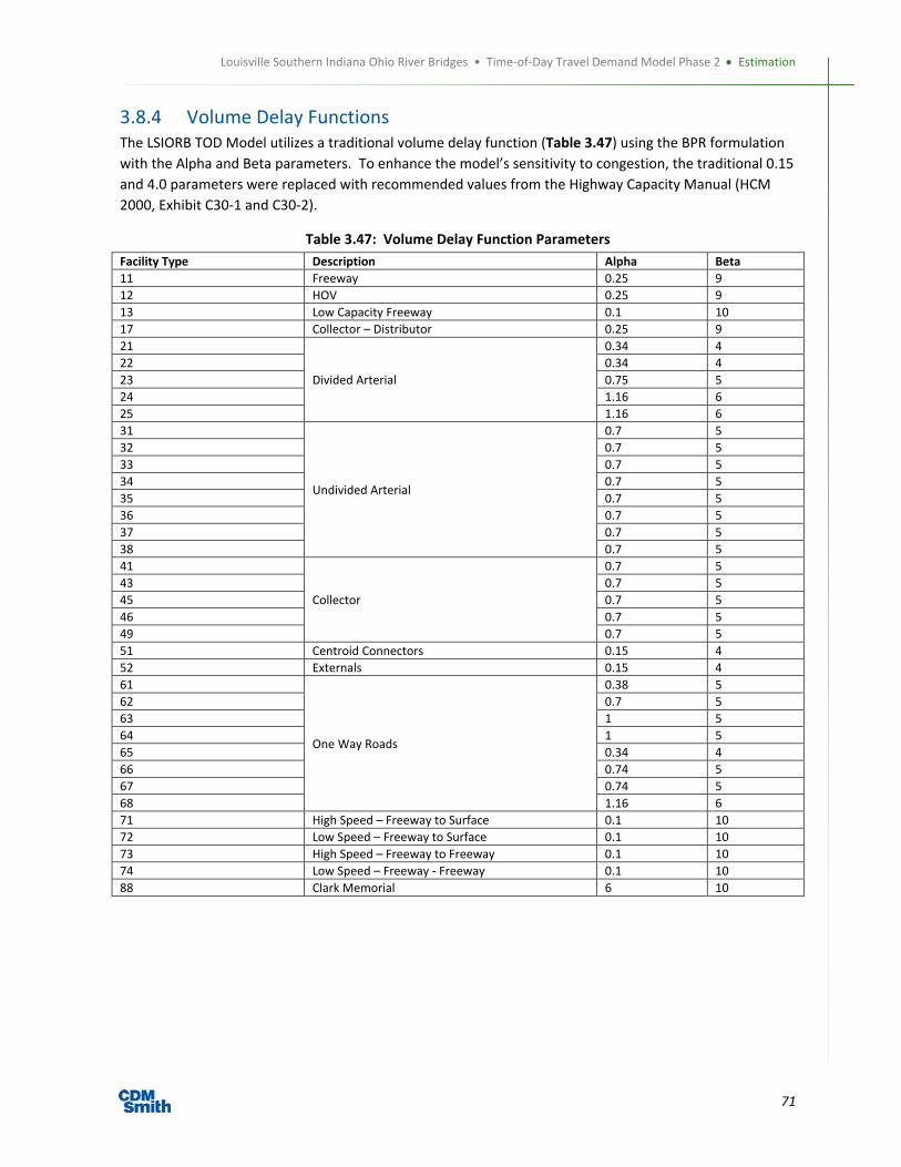
Louisville Southern Indiana Ohio River Bridges • Time‐of‐Day Travel Demand Model Phase 2 Estimation
71
3.8.4 Volume Delay Functions The LSIORB TOD Model utilizes a traditional volume delay function (Table 3.47) using the BPR formulation
with the Alpha and Beta parameters. To enhance the model’s sensitivity to congestion, the traditional 0.15
and 4.0 parameters were replaced with recommended values from the Highway Capacity Manual (HCM
2000, Exhibit C30‐1 and C30‐2).
Table 3.47: Volume Delay Function Parameters
Facility Type Description Alpha Beta
11 Freeway 0.25 9
12 HOV 0.25 9
13 Low Capacity Freeway 0.1 10
17 Collector – Distributor 0.25 9
21
Divided Arterial
0.34 4
22 0.34 4
23 0.75 5
24 1.16 6
25 1.16 6
31
Undivided Arterial
0.7 5
32 0.7 5
33 0.7 5
34 0.7 5
35 0.7 5
36 0.7 5
37 0.7 5
38 0.7 5
41
Collector
0.7 5
43 0.7 5
45 0.7 5
46 0.7 5
49 0.7 5
51 Centroid Connectors 0.15 4
52 Externals 0.15 4
61
One Way Roads
0.38 5
62 0.7 5
63 1 5
64 1 5
65 0.34 4
66 0.74 5
67 0.74 5
68 1.16 6
71 High Speed – Freeway to Surface 0.1 10
72 Low Speed – Freeway to Surface 0.1 10
73 High Speed – Freeway to Freeway 0.1 10
74 Low Speed – Freeway ‐ Freeway 0.1 10
88 Clark Memorial 6 10
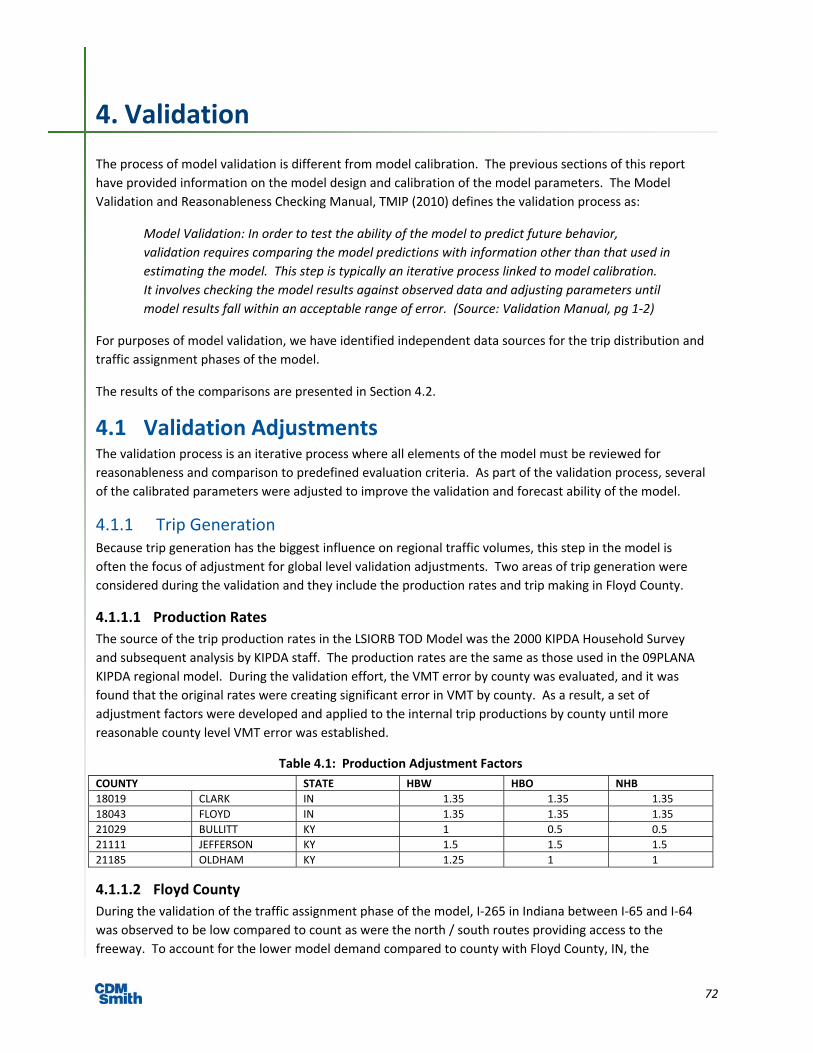
72
4. Validation
The process of model validation is different from model calibration. The previous sections of this report
have provided information on the model design and calibration of the model parameters. The Model
Validation and Reasonableness Checking Manual, TMIP (2010) defines the validation process as:
Model Validation: In order to test the ability of the model to predict future behavior,
validation requires comparing the model predictions with information other than that used in
estimating the model. This step is typically an iterative process linked to model calibration.
It involves checking the model results against observed data and adjusting parameters until
model results fall within an acceptable range of error. (Source: Validation Manual, pg 1‐2)
For purposes of model validation, we have identified independent data sources for the trip distribution and
traffic assignment phases of the model.
The results of the comparisons are presented in Section 4.2.
4.1 Validation Adjustments The validation process is an iterative process where all elements of the model must be reviewed for
reasonableness and comparison to predefined evaluation criteria. As part of the validation process, several
of the calibrated parameters were adjusted to improve the validation and forecast ability of the model.
4.1.1 Trip Generation Because trip generation has the biggest influence on regional traffic volumes, this step in the model is
often the focus of adjustment for global level validation adjustments. Two areas of trip generation were
considered during the validation and they include the production rates and trip making in Floyd County.
4.1.1.1 Production Rates
The source of the trip production rates in the LSIORB TOD Model was the 2000 KIPDA Household Survey
and subsequent analysis by KIPDA staff. The production rates are the same as those used in the 09PLANA
KIPDA regional model. During the validation effort, the VMT error by county was evaluated, and it was
found that the original rates were creating significant error in VMT by county. As a result, a set of
adjustment factors were developed and applied to the internal trip productions by county until more
reasonable county level VMT error was established.
Table 4.1: Production Adjustment Factors
COUNTY STATE HBW HBO NHB
18019 CLARK IN 1.35 1.35 1.35
18043 FLOYD IN 1.35 1.35 1.35
21029 BULLITT KY 1 0.5 0.5
21111 JEFFERSON KY 1.5 1.5 1.5
21185 OLDHAM KY 1.25 1 1
4.1.1.2 Floyd County
During the validation of the traffic assignment phase of the model, I‐265 in Indiana between I‐65 and I‐64
was observed to be low compared to count as were the north / south routes providing access to the
freeway. To account for the lower model demand compared to county with Floyd County, IN, the
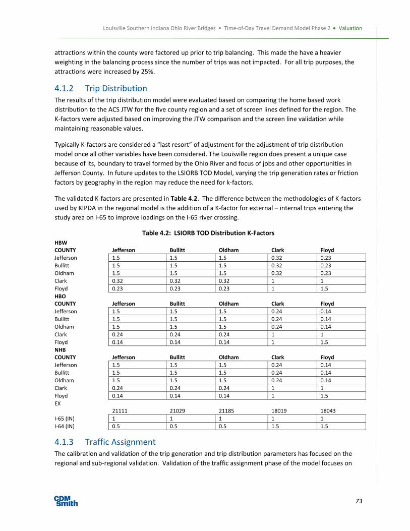
Louisville Southern Indiana Ohio River Bridges • Time‐of‐Day Travel Demand Model Phase 2 Valuation
73
attractions within the county were factored up prior to trip balancing. This made the have a heavier
weighting in the balancing process since the number of trips was not impacted. For all trip purposes, the
attractions were increased by 25%.
4.1.2 Trip Distribution The results of the trip distribution model were evaluated based on comparing the home based work
distribution to the ACS JTW for the five county region and a set of screen lines defined for the region. The
K‐factors were adjusted based on improving the JTW comparison and the screen line validation while
maintaining reasonable values.
Typically K‐factors are considered a “last resort” of adjustment for the adjustment of trip distribution
model once all other variables have been considered. The Louisville region does present a unique case
because of its, boundary to travel formed by the Ohio River and focus of jobs and other opportunities in
Jefferson County. In future updates to the LSIORB TOD Model, varying the trip generation rates or friction
factors by geography in the region may reduce the need for k‐factors.
The validated K‐factors are presented in Table 4.2. The difference between the methodologies of K‐factors
used by KIPDA in the regional model is the addition of a K‐factor for external – internal trips entering the
study area on I‐65 to improve loadings on the I‐65 river crossing.
Table 4.2: LSIORB TOD Distribution K‐Factors
HBW COUNTY Jefferson Bullitt Oldham Clark Floyd
Jefferson 1.5 1.5 1.5 0.32 0.23
Bullitt 1.5 1.5 1.5 0.32 0.23
Oldham 1.5 1.5 1.5 0.32 0.23
Clark 0.32 0.32 0.32 1 1
Floyd 0.23 0.23 0.23 1 1.5
HBO COUNTY Jefferson Bullitt Oldham Clark Floyd
Jefferson 1.5 1.5 1.5 0.24 0.14
Bullitt 1.5 1.5 1.5 0.24 0.14
Oldham 1.5 1.5 1.5 0.24 0.14
Clark 0.24 0.24 0.24 1 1
Floyd 0.14 0.14 0.14 1 1.5
NHB COUNTY Jefferson Bullitt Oldham Clark Floyd
Jefferson 1.5 1.5 1.5 0.24 0.14
Bullitt 1.5 1.5 1.5 0.24 0.14
Oldham 1.5 1.5 1.5 0.24 0.14
Clark 0.24 0.24 0.24 1 1
Floyd 0.14 0.14 0.14 1 1.5
EX 21111 21029 21185 18019 18043
I‐65 (IN) 1 1 1 1 1
I‐64 (IN) 0.5 0.5 0.5 1.5 1.5
4.1.3 Traffic Assignment The calibration and validation of the trip generation and trip distribution parameters has focused on the
regional and sub‐regional validation. Validation of the traffic assignment phase of the model focuses on

Louisville Southern Indiana Ohio River Bridges • Time‐of‐Day Travel Demand Model Phase 2 Valuation
74
the local level or link by link basis. As part of the traffic assignment validation, the following parameters
were considered:
Adjustments to input speeds
Capacity assumptions
4.1.3.1 Speed Adjustments
Section 3.2.1 has documented the assumptions and methodology for calculating the adjusted free flow
speeds. The input to this process was an assumption regarding the speed limit for each link in the network.
Since only speed limit data was available from KYTC and not INDOT, initial runs of the LSIORB TOD Model
used assumptions speed limits by facility type and area type where data was not available. During the
validation, CDM Smith staff made several fields visits to the study to provide existing posted speed limit
data. Particular attention was paid to the I‐64 and I‐265 routes as well as within the Clarksville and New
Albany areas.
4.1.3.2 Capacity Restrictions
The Louisville network has specific locations on the interstate system that are problem areas for
congestion. These include:
I‐65
– South of downtown (“Hospital Curve”)
– I‐65 Memorial Bridge
I‐64
– Cochran Tunnel
– Sherman Minton Bridge
– From I‐264 to I‐65 west of I‐65
CBD
– Default speed was changed to all non‐freeway links within the CBD to 25mph
Clark Memorial
– New facility type (FACT) was established for bridge that included a default speed change
For the above sections, a capacity analysis was completed to evaluate the impact of the increase weave
sections and reduced lane width and shoulders. To account for the impact to capacity, different volume
delay function parameters were applied to the facility type.
4.1.3.3 Clark Memorial Bridge (US 31)
In the development of the LSIORB TOD Model, special attention was paid to the Clark Memorial Bridge
because of special techniques used in the original KIPDA daily model and the importance of US 31 to the
downtown roadway system and as a potential diversion route to I‐65 when tolled.
KIPDA Model
The KIPDA daily model deals with the validation of the Clark Memorial Bridge in different ways including
the use of significant time penalties to balance the traffic crossing the river. Further, the KIPDA model
restricts cross river traffic by defining trips that are intrastate and interstate. The model prohibits the
intrastate trips from using the bridges. This was change was made to prevent any trips from “double
crossing” the river. The 09PLANA model used in previous rounds of analysis on the bridges had a total daily

Louisville Southern Indiana Ohio River Bridges • Time‐of‐Day Travel Demand Model Phase 2 Valuation
75
volume of 17,722 ADT as compared to a year 2000 count of 19,600 vehicles per day (vpd). Further the
model produces an unbalanced flow of more than 11,000 vehicles in the north bound direction.
TOD Model Validation
In the early rounds of the validation, the emphasis was placed on matching the existing count on all three
existing bridges, including the Clark Memorial (US‐31) while not using any special treatments or methods. A
high level of validation was achieved across the three bridges and each bridge in particular without any
special treatments or methods. A thorough review of the roadway attributes on both sides of the river was
undertaken to insure the model reflected the conditions in the field. This included review of traffic signal
locations, number of lanes, concerns with pedestrian crossing, width of the roadway, and any other traffic
control devices that might impede traffic flow (stop signs, traffic calming devices, etc.).
Future Year Validation Testing
The tests completed during the validation indicated that when US 31 was well validated in the base year, it
resulted in unreasonable future forecast volumes, especially under toll conditions when traffic far
exceeded the capacity of the US 31 bridge. The analysis discussed below shows that when I‐65 is tolled,
the model considers US 31 a viable alternative because of the trade off in travel time versus cost in the
generalized cost traffic assignment even though it creates extreme congestion on the bridge. Note that
while the actual distance on I‐65 is longer than US‐31, because of local street connections, narrow lanes
and traffic signals US‐31 is and will continue to be a less attractive route and reaches capacity much faster
than I‐65. Further review determined that when typical volume delay function parameters are used on the
US 31 link, unrealistic volumes were assigned to the bridge because even under extreme congestion, the
travel time was still lower than the time plus cost for I‐65. Ultimately some means to address this over‐
assignment in the future needed to be developed that could be repeated under all future scenarios without
intervention.
Solution
The solution used on US 31 was to create a unique facility type for the link that imposed a more aggressive
volume delay function as compared to the surrounding links.
This choice was made to prevent unreasonable loadings in the forecast, especially when I‐65 is tolled and
not have intervention each time a toll rate is changed. In applying a unique volume delay function, it
would be ideal to estimate the function to existing conditions. Because of the configuration of the Clark
Memorial Bridge with a signal at both ends and the grid roadway network in Louisville, it was not possible
to get realistic travel times on the bridge since the actual delay is related to the signalization. The study
team did look at modeled travel time between US 31 and I‐65 between several zone pairs on both sides of
the river for reasonableness compared to firsthand knowledge of actual travel times.
Alternative solutions were considered including using a static time penalty approach but these would
introduce an additional bias to the analysis. Under a time penalty approach, it would be necessary to
estimate an appropriate value based on the toll rate being tested on I‐65. Since there was no basis for the
penalty in relation to the toll, this would introduce an additional bias.
Results
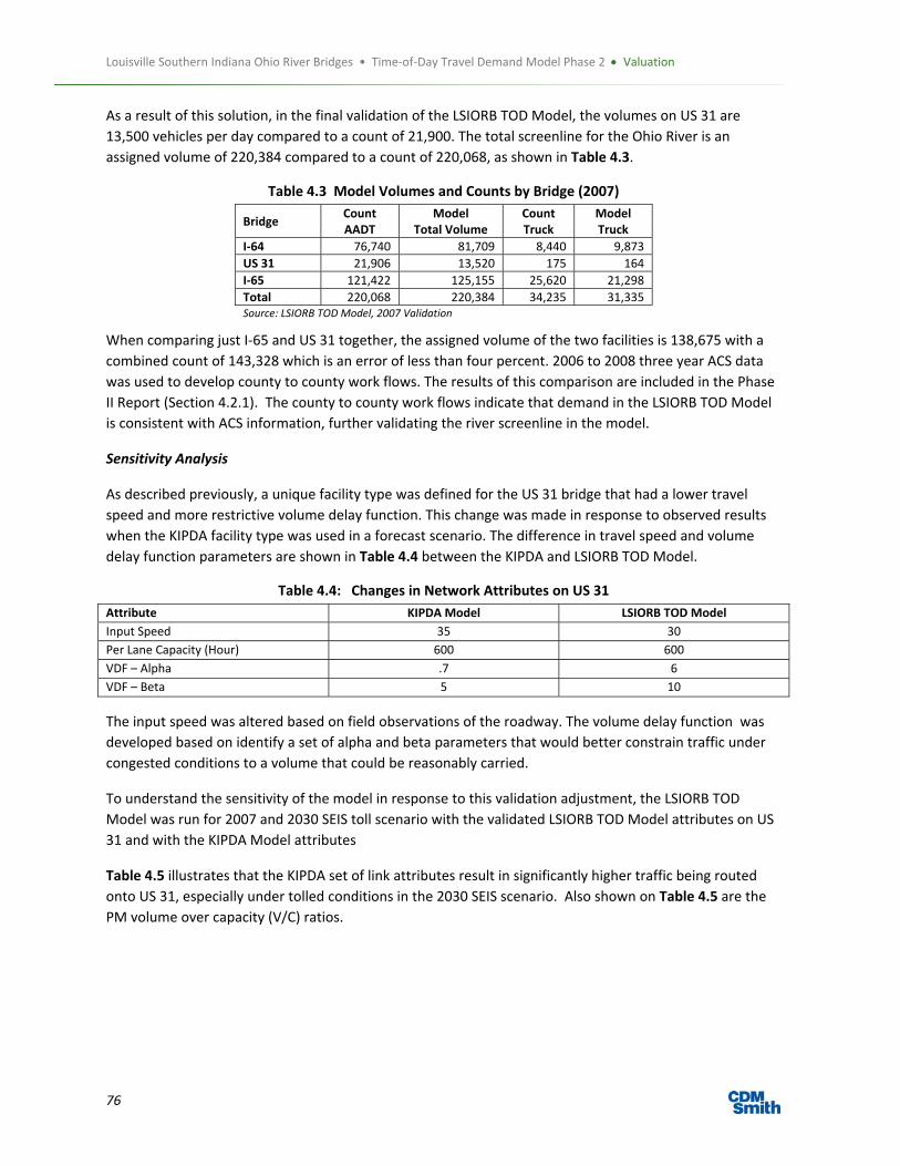
Louisville Southern Indiana Ohio River Bridges • Time‐of‐Day Travel Demand Model Phase 2 Valuation
76
As a result of this solution, in the final validation of the LSIORB TOD Model, the volumes on US 31 are
13,500 vehicles per day compared to a count of 21,900. The total screenline for the Ohio River is an
assigned volume of 220,384 compared to a count of 220,068, as shown in Table 4.3.
Table 4.3 Model Volumes and Counts by Bridge (2007)
Bridge Count AADT
Model Total Volume
Count Truck
Model Truck
I‐64 76,740 81,709 8,440 9,873
US 31 21,906 13,520 175 164
I‐65 121,422 125,155 25,620 21,298
Total 220,068 220,384 34,235 31,335 Source: LSIORB TOD Model, 2007 Validation
When comparing just I‐65 and US 31 together, the assigned volume of the two facilities is 138,675 with a
combined count of 143,328 which is an error of less than four percent. 2006 to 2008 three year ACS data
was used to develop county to county work flows. The results of this comparison are included in the Phase
II Report (Section 4.2.1). The county to county work flows indicate that demand in the LSIORB TOD Model
is consistent with ACS information, further validating the river screenline in the model.
Sensitivity Analysis
As described previously, a unique facility type was defined for the US 31 bridge that had a lower travel
speed and more restrictive volume delay function. This change was made in response to observed results
when the KIPDA facility type was used in a forecast scenario. The difference in travel speed and volume
delay function parameters are shown in Table 4.4 between the KIPDA and LSIORB TOD Model.
Table 4.4: Changes in Network Attributes on US 31
Attribute KIPDA Model LSIORB TOD Model
Input Speed 35 30
Per Lane Capacity (Hour) 600 600
VDF – Alpha .7 6
VDF – Beta 5 10
The input speed was altered based on field observations of the roadway. The volume delay function was
developed based on identify a set of alpha and beta parameters that would better constrain traffic under
congested conditions to a volume that could be reasonably carried.
To understand the sensitivity of the model in response to this validation adjustment, the LSIORB TOD
Model was run for 2007 and 2030 SEIS toll scenario with the validated LSIORB TOD Model attributes on US
31 and with the KIPDA Model attributes
Table 4.5 illustrates that the KIPDA set of link attributes result in significantly higher traffic being routed
onto US 31, especially under tolled conditions in the 2030 SEIS scenario. Also shown on Table 4.5 are the
PM volume over capacity (V/C) ratios.

Louisville Southern Indiana Ohio River Bridges • Time‐of‐Day Travel Demand Model Phase 2 Valuation
77
Table 4.5: Daily Volume by Bridge
2007 2030 SEIS TOLL
Bridge LSIORB PM V/C KIPDA PM V/C LSIORB PM V/C KIPDA PM V/C
I‐64 83,363 1.03 83,262 1.04 121,811 1.41 121,411 1.41
US 31 12,183 0.80 13,542 0.94 35,409 1.00 51,315 1.53
I‐65 126,756 1.29 125,825 1.28 103,160 0.97 87,704 0.90
I‐265 49,582 1.24 49,307 1.24
Total 222,303 222,629 309,961 309,737 Note: LSIORB Attributes – LSIORB TOD US 31 Link Attributes
KIPDA Attributes‐ KIPDA Model US 31 Link Attributes
A volume of 50,000 vehicles per day in 2030 on US 31 was not seen as reasonable during the model
validation, and thus the adjustments shown in Table 4.4 were applied during model validation.
Reasonableness Checks
Several reasonableness checks were applied to determine what the US 31 bridge could actually carry:
Actual ADT is 21,906 (2010 tube count);
Peak hours are 7:00 (1900 PHV); 8:00 (1500 PHV,), 5:00 (2500 PHV) and 6:00 (2650 PHV). The
directional distribution in the AM ranges from 76 SB/24 NB to 83 SB/17 NB. The directional
distribution during the PM ranges from 55 NB/ 45 SB to 60 NB/ 40 SB.
The four top peak hours carry 8,508 vehicles ( 39% of the daily traffic) and the top twelve hours
carry 17,664 (90.6% of the traffic)
The KIPDA capacities for US 31 are 600 per lane which is a little low despite the fact that the access
is signal controlled. The HCM saturated flow rate is 1900 vehicle per lane per hour and with two
lanes and a green time of 45%, a directional capacity of approximately 1,700 (850 per lane) can be
achieved which is higher than KIPDA’s value.
The bridge will likely always have a peak directional flow to reflect the heavy commuting patterns of
southbound in the morning and northbound in the evening.
The hourly capacity of the US 31 bridge can be estimated by taking the per lane capacity times four
to get 3400 (PM capacity = 850 x4).
The total hourly capacity can be used to develop a daily capacity of approximately 34,000 (3400 x
10).
This exercise shows that the actual daily capacity should be 34,000 which is close to what the LSIORB
attributes yield (they actually yield 35,409 during the SEIS toll scenario).
To work back from the 50,000 daily trips on US 31, it would make it necessary to have an hourly capacity
of approximately 5,000 vehicles per hour which clearly is not possible with the existing commuting
patterns (causing the directional split) and the delay caused by traffic signals at both ends of the bridge.
During the 60/40 split hour, this would produce 3,000 trips per hour per direction which could not be
pushed through by the arterial signal system.

Louisville Southern Indiana Ohio River Bridges • Time‐of‐Day Travel Demand Model Phase 2 Valuation
78
Thus the CDM Smith modeling team used engineering judgment based on detailed knowledge of the actual
US 31 capacity to make the decision that 50,000 trips per day on the US 31 bridge is not reasonable.
Trip Distribution Checks
It is important to note from Table 3 that the combined volumes using US 31 and I‐65 under both set
attributes result in nearly identical combined volumes. This indicates that from a distribution perspective,
the change has no impact on the model, but instead only impacts the routing of trips.
To verify this conclusion regarding distribution, the aggregated select link trip table cell values for north
and southbound travel were compared between the two model runs for each year. The daily change in
number of trips from any zone crossing the river using US 31 or I‐65 was less than plus or minus 30 in 2007
and 2030.
Conclusion
Adjustments to the US 31 capacity restraints were made in order to allow the future year model to
make reasonable assignments on US 31 and the Ohio River bridge crossings.
The price for accurate 2030 assignments was to accept slightly inaccurate base year assignments.
These US 31 capacity adjustments are further justified since the current operating conditions of US
31 are close to ultimate capacity and there are no plans to significantly improve capacity with
revised signal plans or geometric improvements.
4.2 Validation Results The validation of the LSIORB TOD Model was an iterative process that included completing in excess of
sixty validation runs to the model. Figure 4.1 shows the improvement to the validation of the model by
plotting the overall percent RMSE for each of the 60+ runs. Percent RMSE is a measure of relative error of
the assignment compared to counts so is useful in showing the improvement of the validation.
Figure 4.1: Percent RMSE of LSIORB TOD Validation
0
10
20
30
40
50
60
70
0 10 20 30 40 50 60 70
PRMSE

Louisville Southern Indiana Ohio River Bridges • Time‐of‐Day Travel Demand Model Phase 2 Valuation
79
Table 4.6 and Table 4.7 provide a description of the parameters that were adjusted for each validation run.
This information is provided to show the depth of the validation exercise and that all portions of the model
were examined in a systematic way.
The traffic counts used for the validation of the LSIORB TOD Model are documented in the Phase I LSIORB
Project Documentation. In total, over thirteen hundred counts were identified and used for validation
purposes. Of that total, 558 included information about truck volumes and 843 included data about hourly
traffic patterns.
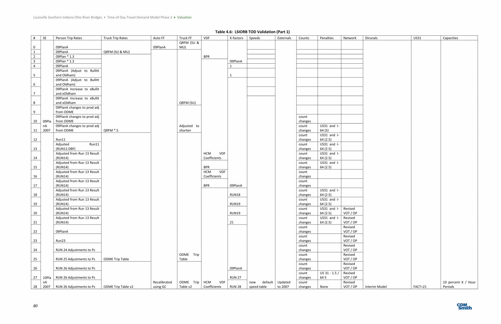
Louisville Southern Indiana Ohio River Bridges • Time‐of‐Day Travel Demand Model Phase 2 Valuation
80
Table 4.6: LSIORB TOD Validation (Part 1)
# SE Person Trip Rates Truck Trip Rates Auto FF Truck FF VDF K‐factors Speeds Externals Counts Penalties Network Dirunals US31 Capacities
0
09PlanA 2007
09PlanA
QRFM (SU & MU)
09PlanA QRFM (SU & MU)
BPR
09PlanA
Updated to 2007
Interim Model FACT=21 10 percent K / Hour Periods
1 09PlanA
Recalibrated using GC
QRFM (SU)
2 09Plan * 1.3
QRFM *.5
3 09Plan * 1.3
HCM VDF Coefficients
4 09PlanA 1
5 09PlanA (Adjust to Bullitt and Oldham) 1
6 09PlanA (Adjust to Bullitt and Oldham)
09PlanA
7 09PlanA Increase to xBullit and xOldham
8 09PlanA Increase to xBullit and xOldham
new default speed table
9 09PlanA changes to prod adj from ODME
Adjusted to shorten
10 09PlanA changes to prod adj from ODME
count changes
11 09PlanA changes to prod adj from ODME
count changes
US31 and I‐64 (5)
12
10PlanA 2007
Run11
ODME Trip Table ODME Trip Table
count changes
US31 and I‐64 (2.5)
13 Adjusted Run11 (RUN12.DBF)
count changes
US31 and I‐64 (2.5)
14 Adjusted from Run 13 Result (RUN14)
count changes
US31 and I‐64 (2.5)
15 Adjusted from Run 13 Result (RUN14) BPR
count changes
US31 and I‐64 (2.5)
16 Adjusted from Run 13 Result (RUN14)
HCM VDF Coefficients
count changes
17 Adjusted from Run 13 Result (RUN14) BPR
count changes
18 Adjusted from Run 13 Result (RUN14)
HCM VDF Coefficients
RUN18 count changes
US31 and I‐64 (2.5)
19 Adjusted from Run 13 Result (RUN14) RUN19
count changes
US31 and I‐64 (2.5)
20 Adjusted from Run 13 Result (RUN14) RUN19
count changes
US31 and I‐64 (2.5)
Revised VOT / OP
21 Adjusted from Run 13 Result (RUN14) 21
count changes
US31 and I‐64 (2.5)
Revised VOT / OP
22 09PlanA
09PlanA
count changes
Revised VOT / OP
23 Run23 count changes
Revised VOT / OP
24 RUN 24 Adjustments to Ps count changes
Revised VOT / OP
25 RUN 25 Adjustments to Ps count changes
Revised VOT / OP
26 RUN 26 Adjustments to Ps
ODME Trip Table v2 ODME Trip Table v2
count changes
Revised VOT / OP
27 RUN 26 Adjustments to Ps RUN 27 count changes
US 31 ‐ 1.5 / 64 5
Revised VOT / OP
28 RUN 26 Adjustments to Ps RUN 28 count changes None
Revised VOT / OP

Louisville Southern Indiana Ohio River Bridges • Time‐of‐Day Travel Demand Model Phase 2 Valuation
81
# SE Person Trip Rates Truck Trip Rates Auto FF Truck FF VDF K‐factors Speeds Externals Counts Penalties Network Dirunals US31 Capacities
29 RUN 26 Adjustments to Ps RUN 28 count changes
US 31 ‐ 1.5 / 64 5
Revised VOT / OP
30 RUN 26 Adjustments to Ps ODME Trip Table 2 * .75 Internal RUN 28
count changes
US 31 ‐ 1.5 / 64 5
Revised VOT / OP
31 RUN 26 Adjustments to Ps ODME Trip Table 2 * .75 Internal (balanced) RUN 28
counts (3/22/11)
US 31 ‐ 2.5 / 64 5
Revised VOT / OP
32
33
34 RUN 26 Adjustments to Ps ODME Trip Table 2 *.75 Int Bal Removal of EE RUN 28
counts (3/22/11)
US 31 ‐ 2.5 / 64 5
Revised VOT / OP
Revised HH Analysis 35 RUN 26 Adjustments to Ps ODME Trip Table 2 *.75 Int Bal Removal of EE RUN 28
counts (3/22/11)
US 31 ‐ 2.5 / 64 2.5
Revised VOT / OP
36 RUN 26 Adjustments to Ps ODME Trip Table 2 *.75 Int Bal Removal of EE RUN 28
counts (3/22/11)
US 31 ‐ 2.5 / 64 5
Revised VOT / OP
Revised HH Analysis / II Trk uses Counts Dist
37 RUN 26 Adjustments to Ps ODME Trip Table 2 *.75 Int Bal Removal of EE RUN 28
counts (3/22/11)
US 31 ‐ 2.5 / 64 5
Revised VOT / OP
38 RUN 26 Adjustments to Ps ODME Trip Table 2 *.75 Int Bal Removal of EE
09PlanA
counts (3/22/11) None
Revised VOT / OP
39 RUN 25 Adjustments to Ps 2007 Truck ODME 2007 Truck ODME
BPR VDF
Counts 3/22/11 None
Revised VOT / OP
LA RUN 25 Adjustments to Ps 2007 Truck ODME 2007 Truck ODME
new def speeds / 25mph Core
Counts 3/22/11 None
Revised VOT / OP US 31 ‐ FACT88
8 percent K / peak period factors
40 RUN 25 Adjustments to Ps 2007 Truck ODME 2007 Truck ODME
Counts 3/22/11 None
Revised VOT / OP
US 31 ‐ FACT36 / 25 MPH
41 RUN 25 Adjustments to Ps 2007 Truck ODME 2007 Truck ODME
Counts 3/22/11 None
Revised VOT / OP
US 31 ‐ FACT36 / 35 MPH
42 RUN 25 Adjustments to Ps 2007 Truck ODME 2007 Truck ODME
Counts 3/22/11 None
Revised VOT / OP
US 31 ‐ FACT88 / 35 MPH
43 RUN 25 Adjustments to Ps 2007 Truck ODME 2007 Truck ODME
Counts 3/22/11 None
Revised VOT / OP
US 31 ‐ FACT36 / 30 MPH
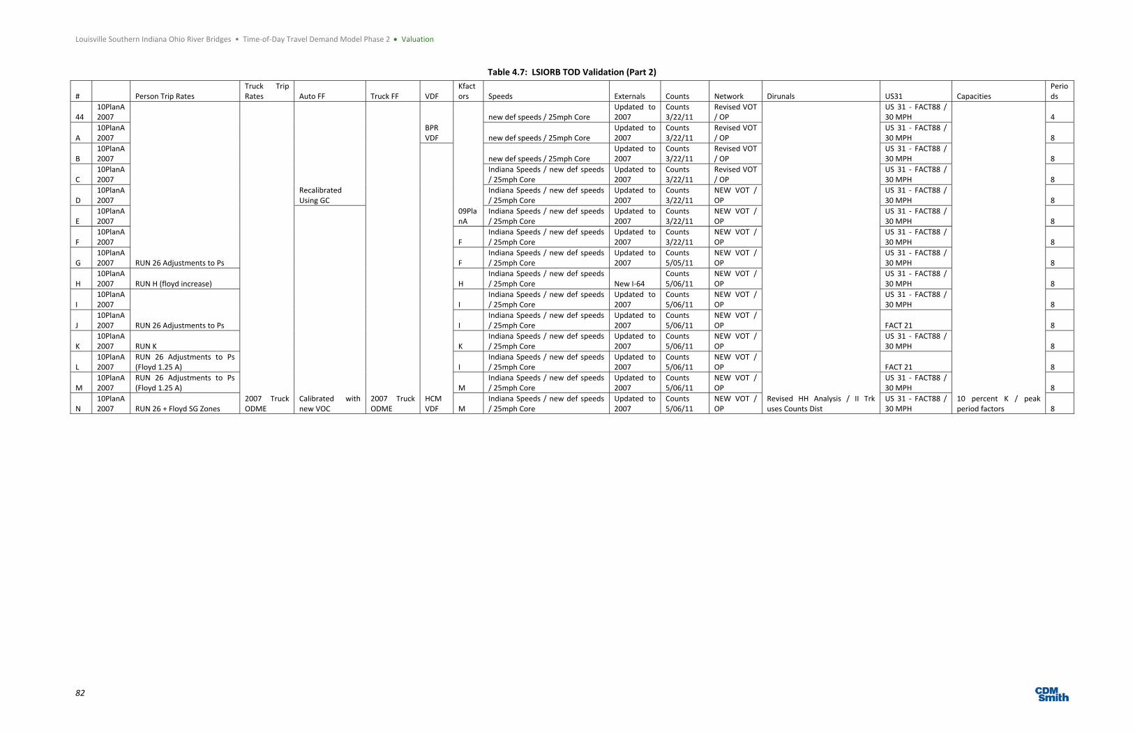
Louisville Southern Indiana Ohio River Bridges • Time‐of‐Day Travel Demand Model Phase 2 Valuation
82
Table 4.7: LSIORB TOD Validation (Part 2)
# Person Trip Rates Truck Trip Rates Auto FF Truck FF VDF
Kfactors Speeds Externals Counts Network Dirunals US31 Capacities
Periods
44 10PlanA 2007
RUN 26 Adjustments to Ps
2007 Truck ODME
Recalibrated Using GC
2007 Truck ODME
BPR VDF
09PlanA
new def speeds / 25mph Core Updated to 2007
Counts 3/22/11
Revised VOT / OP
Revised HH Analysis / II Trk uses Counts Dist
US 31 ‐ FACT88 / 30 MPH
10 percent K / peak period factors
4
A 10PlanA 2007 new def speeds / 25mph Core
Updated to 2007
Counts 3/22/11
Revised VOT / OP
US 31 ‐ FACT88 / 30 MPH 8
B 10PlanA 2007
HCM VDF
new def speeds / 25mph Core Updated to 2007
Counts 3/22/11
Revised VOT / OP
US 31 ‐ FACT88 / 30 MPH 8
C 10PlanA 2007
Indiana Speeds / new def speeds / 25mph Core
Updated to 2007
Counts 3/22/11
Revised VOT / OP
US 31 ‐ FACT88 / 30 MPH 8
D 10PlanA 2007
Indiana Speeds / new def speeds / 25mph Core
Updated to 2007
Counts 3/22/11
NEW VOT / OP
US 31 ‐ FACT88 / 30 MPH 8
E 10PlanA 2007
Calibrated with new VOC
Indiana Speeds / new def speeds / 25mph Core
Updated to 2007
Counts 3/22/11
NEW VOT / OP
US 31 ‐ FACT88 / 30 MPH 8
F 10PlanA 2007 F
Indiana Speeds / new def speeds / 25mph Core
Updated to 2007
Counts 3/22/11
NEW VOT / OP
US 31 ‐ FACT88 / 30 MPH 8
G 10PlanA 2007 F
Indiana Speeds / new def speeds / 25mph Core
Updated to 2007
Counts 5/05/11
NEW VOT / OP
US 31 ‐ FACT88 / 30 MPH 8
H 10PlanA 2007 RUN H (floyd increase) H
Indiana Speeds / new def speeds / 25mph Core New I‐64
Counts 5/06/11
NEW VOT / OP
US 31 ‐ FACT88 / 30 MPH 8
I 10PlanA 2007
RUN 26 Adjustments to Ps
I Indiana Speeds / new def speeds / 25mph Core
Updated to 2007
Counts 5/06/11
NEW VOT / OP
US 31 ‐ FACT88 / 30 MPH 8
J 10PlanA 2007 I
Indiana Speeds / new def speeds / 25mph Core
Updated to 2007
Counts 5/06/11
NEW VOT / OP FACT 21 8
K 10PlanA 2007 RUN K K
Indiana Speeds / new def speeds / 25mph Core
Updated to 2007
Counts 5/06/11
NEW VOT / OP
US 31 ‐ FACT88 / 30 MPH 8
L 10PlanA 2007
RUN 26 Adjustments to Ps (Floyd 1.25 A) I
Indiana Speeds / new def speeds / 25mph Core
Updated to 2007
Counts 5/06/11
NEW VOT / OP FACT 21 8
M 10PlanA 2007
RUN 26 Adjustments to Ps (Floyd 1.25 A) M
Indiana Speeds / new def speeds / 25mph Core
Updated to 2007
Counts 5/06/11
NEW VOT / OP
US 31 ‐ FACT88 / 30 MPH 8
N 10PlanA 2007 RUN 26 + Floyd SG Zones M
Indiana Speeds / new def speeds / 25mph Core
Updated to 2007
Counts 5/06/11
NEW VOT / OP
US 31 ‐ FACT88 / 30 MPH 8
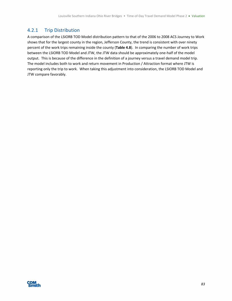
Louisville Southern Indiana Ohio River Bridges • Time‐of‐Day Travel Demand Model Phase 2 Valuation
83
4.2.1 Trip Distribution A comparison of the LSIORB TOD Model distribution pattern to that of the 2006 to 2008 ACS Journey to Work
shows that for the largest county in the region, Jefferson County, the trend is consistent with over ninety
percent of the work trips remaining inside the county (Table 4.8). In comparing the number of work trips
between the LSIORB TOD Model and JTW, the JTW data should be approximately one‐half of the model
output. This is because of the difference in the definition of a journey versus a travel demand model trip.
The model includes both to work and return movement in Production / Attraction format where JTW is
reporting only the trip to work. When taking this adjustment into consideration, the LSIORB TOD Model and
JTW compare favorably.

Louisville Southern Indiana Ohio River Bridges • Time‐of‐Day Travel Demand Model Phase 2 Valuation
84
Table 4.8: ACS JTW (2006‐2008)
ACS JTW (2006‐2008) LSIORB JTW
RESIDENCE
WORKPLACE WORKPLACE
Clark Floyd Bullitt Jefferson Oldham Total
Clark Floyd Bullitt Jefferson Oldham Total
IN IN KY KY KY IN IN KY KY KY
Clark IN 24,275 6,755 140 18,020 295 49,485 40,527 17,179 422 22,709 474 81,311
Floyd IN 6,655 14,910 95 12,615 115 34,390 15,406 31,083 195 10,448 206 57,338
Bullitt KY 370 270 9,740 23,330 195 33,905 1,021 412 8,360 32,222 750 42,765
Jefferson KY 6,365 2,015 3,215 305,805 2,745 320,145 18,217 9,215 15,660 548,616 13,776 605,485
Oldham KY 235 70 50 15,595 8,190 24,140 970 391 543 26,065 10,614 38,583
Total 37,900 24,020 13,240 375,365 11,540 ‐ 76,141 58,280 25,180 640,060 25,820 ‐
ACS JTW (2006‐2008) LSIORB JTW
RESIDENCE
WORKPLACE WORKPLACE
Clark Floyd Bullitt Jefferson Oldham Total
Clark Floyd Bullitt Jefferson Oldham Total
IN IN KY KY KY IN IN KY KY KY
Clark IN 49.10% 13.70% 0.30% 36.40% 0.60% 100% 49.80% 21.10% 0.50% 27.90% 0.60% 100%
Floyd IN 19.40% 43.40% 0.30% 36.70% 0.30% 100% 26.90% 54.20% 0.30% 18.20% 0.40% 100%
Bullitt KY 1.10% 0.80% 28.70% 68.80% 0.60% 100% 2.40% 1.00% 19.50% 75.30% 1.80% 100%
Jefferson KY 2.00% 0.60% 1.00% 95.50% 0.90% 100% 3.00% 1.50% 2.60% 90.60% 2.30% 100%
Oldham KY 1.00% 0.30% 0.20% 64.60% 33.90% 100% 2.50% 1.00% 1.40% 67.60% 27.50% 100%
Total 100% 100% 100% 100% 100% ‐ 100% 100% 100% 100% 100% ‐

Louisville Southern Indiana Ohio River Bridges • Time‐of‐Day Travel Demand Model Phase 2 Valuation
85
4.2.2 Daily Assignment Validation The output of the traffic assignment validation for the 24‐hour period includes the following metrics:
Absolute VMT Error
– Facility Type group
– Area Type
– County
Percent RMSE
– Volume Group
Total Traffic Volume
– Ohio River Bridges
– Screenline Analysis
For each metric, the LSIORB TOD Model (TOD) is compared against a criteria and the 09PLANA Daily model
(DAILY) and the 09PLANA Interim TOD Model (INTERIM). The distribution of counts by facility type, area
type and county are shown in Table 4.9.
Table 4.9: Number of Validation Counts by Facility Type, Area Type and County
Facility Counts Area Type Count County Counts Screenline Counts
FREEWAY 181 11 44 Bullitt 98 1 2
DIV ART 180 12 12 Clark 184 2 7
UDIV ART 406 21 53 Floyd 120 3 7
LOCAL 350 31 211 Jefferson 772 4 9
ONE WAY 90 41 601 Oldham 92 5 18
RAMPS 58 43 61 6 7
45 26 7 1
51 6 8 2
53 36
55 217
Figure 4.2 shows the over and under assigned volumes on a daily basis for the validation.

Louisville Southern Indiana Ohio River Bridges • Time‐of‐Day Travel Demand Model Phase 2 Valuation
86
Figure 4.2: LSIORB TOD Model – Daily Validation

Louisville Southern Indiana Ohio River Bridges • Time‐of‐Day Travel Demand Model Phase 2 Valuation
87
The following criteria are based on the calculation of absolute error between the modeled VMT and the
counted VMT on links with counts. The modeled VMT equals the model assignment times the link
distance. The counted VMT equals the traffic count times the link distance. The data is compared by
facility type and area type.
For each metric, figures are provided below that show the criteria, and the performance of the KIPDA daily
model (DAILY), the interim time of day model developed by Wilbur Smith using the daily model (INTERIM),
and finally the LSIORB TOD Model (TOD).
The criteria established for the facility type groups is based on FHWA and Ohio Department of
Transportation guidelines for travel demand model validation. As the average roadway volume decreases
for lesser facility types, the criterion is more relaxed. The criterion applied is the absolute VMT error
between counted and modeled VMT on links with counts. The criterion ranges from a low of 7% for
freeways to 15% for local streets. Figure 4.3 demonstrates that for all facility type groups with the
exception of one way roadways, the LSIORB TOD Model is below the established criteria. One way
roadways exceed the criteria (10% vs 12%).
Figure 4.3: Absolute Error of Counted vs. Modeled VMT by Facility Type Group
Area Type validation is based on the zonal area types assigned by the KIPDA 09PLANA Model. A criterion of
10% absolute VMT error was set for all area types. The LSIORB TOD Model improves the validation for
nearly all area types with the exception of CBD. (Figure 4.4)
0
2
4
6
8
10
12
14
16
CRITERIA
DAILY
INTERIM
TOD
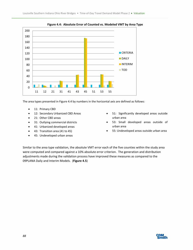
Louisville Southern Indiana Ohio River Bridges • Time‐of‐Day Travel Demand Model Phase 2 Valuation
88
Figure 4.4: Absolute Error of Counted vs. Modeled VMT by Area Type
The area types presented in Figure 4.4 by numbers in the horizontal axis are defined as follows:
11: Primary CBD
12: Secondary Urbanized CBD Areas
21: Other CBD areas
31: Outlying commercial districts
41: Urbanized developed areas
43: Transition area (41 to 45)
45: Undeveloped urban areas
51: Significantly developed areas outside
urban area
53: Small developed areas outside of
urban area
55: Undeveloped areas outside urban area
Similar to the area type validation, the absolute VMT error each of the five counties within the study area
were computed and compared against a 10% absolute error criterion. The generation and distribution
adjustments made during the validation process have improved these measures as compared to the
09PLANA Daily and Interim Models. (Figure 4.5)
0
20
40
60
80
100
120
140
160
180
200
11 12 21 31 41 43 45 51 53 55
CRITERIA
DAILY
INTERIM
TOD
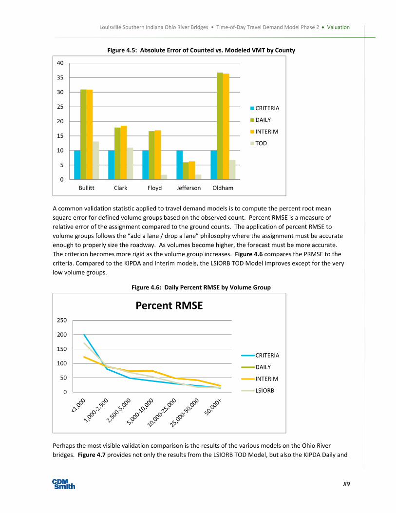
Louisville Southern Indiana Ohio River Bridges • Time‐of‐Day Travel Demand Model Phase 2 Valuation
89
Figure 4.5: Absolute Error of Counted vs. Modeled VMT by County
A common validation statistic applied to travel demand models is to compute the percent root mean
square error for defined volume groups based on the observed count. Percent RMSE is a measure of
relative error of the assignment compared to the ground counts. The application of percent RMSE to
volume groups follows the “add a lane / drop a lane” philosophy where the assignment must be accurate
enough to properly size the roadway. As volumes become higher, the forecast must be more accurate.
The criterion becomes more rigid as the volume group increases. Figure 4.6 compares the PRMSE to the
criteria. Compared to the KIPDA and Interim models, the LSIORB TOD Model improves except for the very
low volume groups.
Figure 4.6: Daily Percent RMSE by Volume Group
Perhaps the most visible validation comparison is the results of the various models on the Ohio River
bridges. Figure 4.7 provides not only the results from the LSIORB TOD Model, but also the KIPDA Daily and
0
5
10
15
20
25
30
35
40
Bullitt Clark Floyd Jefferson Oldham
CRITERIA
DAILY
INTERIM
TOD
0
50
100
150
200
250
Percent RMSE
CRITERIA
DAILY
INTERIM
LSIORB

Louisville Southern Indiana Ohio River Bridges • Time‐of‐Day Travel Demand Model Phase 2 Valuation
90
Interim TOD Models compared to the 2000 traffic counts. The figure also provides a breakdown of traffic
by direction on I‐65 and I‐64.
Figure 4.7: Daily River Crossings by Bridge
In conjunction with the Ohio River bridges, eight additional screenlines were identified to capture the
movement of vehicles across the river and between counties in the region as well as trip in and out of the
CBD. The screenlines as depicted in Figure 4.8 were developed based on the location of counts in the
network. Screenline Validation is shown in Table 4.10.
0
10,000
20,000
30,000
40,000
50,000
60,000
70,000
I‐64EB I‐64WB Clark Mem I‐65 SB I‐65 NB
2000
DAILY
INTERIM
2007
LSIORB
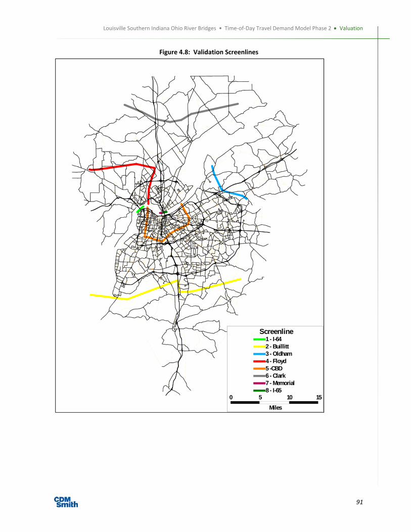
Louisville Southern Indiana Ohio River Bridges • Time‐of‐Day Travel Demand Model Phase 2 Valuation
91
Figure 4.8: Validation Screenlines
0 5 10 15
Miles
Screenline1 - I-642 - Buillitt3 - Oldham4 - Floyd5 -CBD6 - Clark7 - Memorial8 - I-65

Louisville Southern Indiana Ohio River Bridges • Time‐of‐Day Travel Demand Model Phase 2 Valuation
92
Table 4.10. Screenline Validation
SCREENLINE DLY AADT
DLY ASSIGN
ERROR DLY
TRK AADT
TRK ASSIGN
ERROR TRK
1 76,740 83,363 8.6 8,440 9,962 18.0
2 157,255 215,289 36.9 56,175 50,686 ‐9.8
3 103,924 114,968 10.6 12,847 12,292 ‐4.3
4 97,396 104,775 7.6 5,980 6,316 5.6
5 454,133 445,415 ‐1.9 41,257 42,857 3.9
6 57,206 64,516 12.8 15,794 17,769 12.5
7 21,906 12,183 ‐44.4 175 136.8512 ‐21.9
8 121,422 126,756 4.4 25,620 21,320 ‐16.8
4.2.3 Validation by Period The validation statistics up to this point have focused on daily total traffic. Because the LSIORB TOD Model
develops traffic by four time periods (AM, MD, PM and NT), it is important to assess the reliability of the
period volumes as well.
From a global perspective, the distribution of internal trips is consistent with the distribution of traffic
through the day as seen in Table 4.11. The difference between the total traffic in the model (MODEL) and
the traffic generated by the internal trips is made up of the external and truck movements.
Table 4.11: Period Distribution of Traffic (Count vs. Model)
Period HBW HBO NHB All
Internal Trips COUNT MODEL
AM (6 ‐ 9) 21.9% 8.4% 3.1% 9.9% 17.9% 21.0%
Mid (9 ‐ 3) 27.4% 34.5% 47.7% 36.2% 32.4% 30.6%
PM (3 ‐ 6) 17.0% 25.7% 28.7% 24.6% 23.1% 25.4%
Overnight 33.7% 31.4% 20.5% 20.4% 26.6% 23.0%
Table 4.12 reports the total counted and modeled VMT by period and facility group along with the overall
percent error by period. The number of counts used to generate the period validation is less than that
used for the daily validation since not all count locations included hourly information.

Louisville Southern Indiana Ohio River Bridges • Time‐of‐Day Travel Demand Model Phase 2 Valuation
93
Table 4.12. VMT Error by Facility Group by Period
PERIOD COUNT MODEL ERROR
AM 1,586,154 1,807,673 14.0%
MD 2,875,568 2,627,821 ‐8.6%
PM 2,044,665 2,185,377 6.9%
NT 2,363,901 1,974,908 ‐16.5%
AM COUNT MODEL ERROR
FREEWAY 1,119,990 1,248,030 11.4%
DIV ART 116,221 138,991 19.6%
UDIV ART 216,814 252,890 16.6%
LOCAL 86,035 119,695 39.1%
ONE WAY 14,950 15,279 2.2%
RAMPS 28,628 30,180 5.4%
Total 1,582,638 1,805,064 14.1%
MD COUNT MODEL ERROR
FREEWAY 1,942,201 1,829,491 ‐5.8%
DIV ART 241,791 196,450 ‐18.8%
UDIV ART 437,709 373,491 ‐14.7%
LOCAL 163,164 161,962 ‐0.7%
ONE WAY 32,934 20,251 ‐38.5%
RAMPS 52,838 43,355 ‐17.9%
Total 2,870,637 2,625,001 ‐8.6%
PM COUNT MODEL ERROR
FREEWAY 1,388,184 1,495,013 7.7%
DIV ART 163,808 174,937 6.8%
UDIV ART 305,050 307,476 0.8%
LOCAL 125,816 151,514 20.4%
ONE WAY 20,330 18,484 ‐9.1%
RAMPS 35,500 34,072 ‐4.0%
Total 2,038,689 2,181,496 7.0%
NT COUNT MODEL ERROR
FREEWAY 1,651,006 1,383,570 ‐16.2%
DIV ART 182,689 145,715 ‐20.2%
UDIV ART 329,448 272,011 ‐17.4%
LOCAL 140,426 124,303 ‐11.5%
ONE WAY 19,719 14,772 ‐25.1%
RAMPS 36,713 32,539 ‐11.4%
Total 2,360,001 1,972,910 ‐16.4%
Figure 4.9 through Figure 4.12 display the information from the above table graphically.

Louisville Southern Indiana Ohio River Bridges • Time‐of‐Day Travel Demand Model Phase 2 Valuation
94
Figure 4.9: AM VMT by Facility Group (Count vs. Model)
Figure 4.10: MD VMT by Facility Group (Count vs. Model)
Figure 4.11: AM VMT by Facility Group (Count vs. Model)
Figure 4.12: AM VMT by Facility Group (Count vs. Model)
0
200,000
400,000
600,000
800,000
1,000,000
1,200,000
1,400,000
10 20 30 40 60 70
AM VMT by Facility Group
COUNT
MODEL
0
500,000
1,000,000
1,500,000
2,000,000
2,500,000
10 20 30 40 60 70
MD VMT by Facility Group
COUNT
MODEL
0
200,000
400,000
600,000
800,000
1,000,000
1,200,000
1,400,000
1,600,000
10 20 30 40 60 70
PM VMT by Facility Group
COUNT
MODEL
0
500,000
1,000,000
1,500,000
2,000,000
10 20 30 40 60 70
NT VMT by Facility Group
COUNT
MODEL
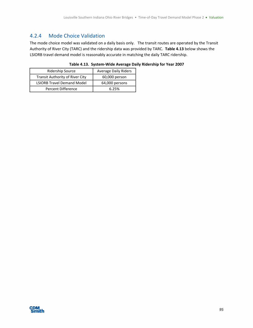
Louisville Southern Indiana Ohio River Bridges • Time‐of‐Day Travel Demand Model Phase 2 Valuation
95
4.2.4 Mode Choice Validation The mode choice model was validated on a daily basis only. The transit routes are operated by the Transit
Authority of River City (TARC) and the ridership data was provided by TARC. Table 4.13 below shows the
LSIORB travel demand model is reasonably accurate in matching the daily TARC ridership.
Table 4.13. System‐Wide Average Daily Ridership for Year 2007
Ridership Source Average Daily Riders
Transit Authority of River City 60,000 person
LSIORB Travel Demand Model 64,000 persons
Percent Difference 6.25%

96
5. Implementation
A GISDK script was developed along with a graphical user interface (GUI) to manage scenario input and output
files as well as post processing model output data. The GISDK script includes all model processes from trip
generation to traffic assignment plus post processing of the model output data and a customized graphical user
interface for the LSIORB project. The GUI has three main components:
1. Scenario Manager 2. Scenario Model Run 3. Scenario Outputs
Each of these components contains various functions specific to managing, running, and analyzing the
LSIORB travel demand model.
5.1 GISDK Interface The LSIORB interface is a customized GISDK graphical user interface developed as an “Add‐In” to the
TransCAD program. The main screen of the LSIORB GUI is shown in Figure 5.1. This dialog box displays an
image of the study area along with three sub dialog boxes available to the user. This box will allow the user
to navigate to the three sub components of the GUI and it will be the “Home Screen” for the model. From
this dialog box, the user will access the Scenario Manager, Scenario Model Run and Scenario Outputs
boxes. For each of the three sub components, the user will specify a scenario which is defined by a scenario
array file (.scn). This file contains all scenario specific descriptions, parameters, and input and output file
names and locations.

Louisville Southern Indiana Ohio River Bridges • Time‐of‐Day Travel Demand Model Phase 2 Implementation
97
Figure 5.1: LSIORB Interface Welcome Screen
The Scenario Manager component of the LSIORB interface allows the user to setup and manage scenarios,
specify parameter values and specify input, interim, and output file names and locations. An image of the
Scenario Manager is shown in Figure 5.2. There are six tabs within the Scenario Manager that allow the
user to specify scenario features. These tabs include:
The “Scenario Settings” tab allows the user to create, copy, delete, and load a predefined scenario. When
creating a new scenario the scenario folder and input files will be based on a defined scenario located in
the “Inputs” folder of the model files or copied based on an existing scenario. Note that the highway and
transit system are specific to each scenario. Thus, scenario specific input folder have been created.
The “Global Parameters” tab allows the user to specify values and flags of various parameters and criteria
including (1) trip generation factors by income level, (2) value of time and operating costs, (3) assignment
and feedback iterations and convergence, (4) network criteria, and (5) various flags to turn on or off truck
and tolling features.
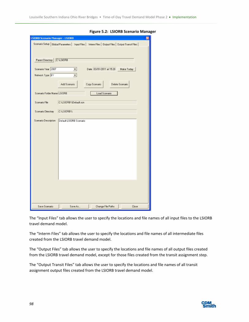
Louisville Southern Indiana Ohio River Bridges • Time‐of‐Day Travel Demand Model Phase 2 Implementation
98
Figure 5.2: LSIORB Scenario Manager
The “Input Files” tab allows the user to specify the locations and file names of all input files to the LSIORB
travel demand model.
The “Interm Files” tab allows the user to specify the locations and file names of all intermediate files
created from the LSIORB travel demand model.
The “Output Files” tab allows the user to specify the locations and file names of all output files created
from the LSIORB travel demand model, except for those files created from the transit assignment step.
The “Output Transit Files” tab allows the user to specify the locations and file names of all transit
assignment output files created from the LSIORB travel demand model.

Louisville Southern Indiana Ohio River Bridges • Time‐of‐Day Travel Demand Model Phase 2 Implementation
99
From each of the six tabs the user can at any time save the existing scenario, save the scenario as a new
scenario, change the directory path of the input and output files (note that this is performed for all tabs at
once), and close out of the Scenario Manager to return to the main screen of the LSIORB interface.
The Scenario Model Run component of the LSIORB interface controls the running of the model and allows
the user to run a single scenario or multiple (up to five) scenarios at once using feedback. Additionally, an
assignment option is provided to allow the user to run traffic assignment with select link analysis. An image
of the Scenario Model Run dialog box is shown in Figure 5.3. Prior to a model run the user must select a
run type (single or multiple model run) and load an existing scenario. The close option from this dialog box
will close out of the Scenario Model Run to return to the main screen of the LSIORB interface.
Figure 5.3: LSIORB Scenario Model Run
The Scenario Outputs component of the LSIORB interface allows the user to view results of the validated
model, post process output data, and view maps of the study area. An image of the Scenario Outputs
dialog box is shown in Figure 5.4. There are three tabs within the Scenario Outputs dialog box that allow
the user to view model outputs. These tabs include:
The “View Outputs” tab allows the user to perform various validation statistics for autos and trucks in the
morning and evening peak periods as well as daily. Such validation statistics include count vs. model vehicle
miles traveled and volume, root mean square error, NCHRP deviation curve, and screenline analysis.
The “Post Processing Options” tab allows the user to update and summarize output data from an existing
model run. Such options include the (1) creation morning and evening peak hour and period table
summaries of the free flow and congested speeds, truck percentages, and traffic counts, (2) the update of
transit drive access links with connecting centriod node identification numbers so that the actual travel
time from the centroid node to the park and ride lot can be updated in the model stream (note that this
only needs to be preformed if a new drive access link is created), and (3) creation of daily, morning, and
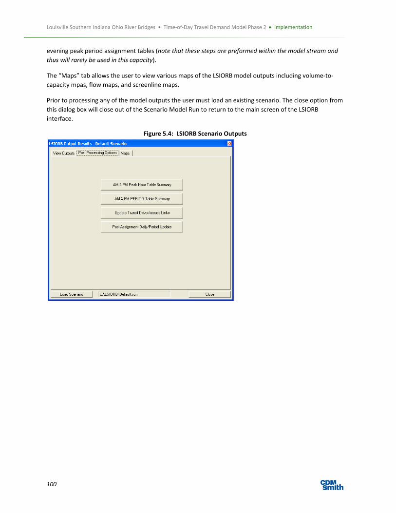
Louisville Southern Indiana Ohio River Bridges • Time‐of‐Day Travel Demand Model Phase 2 Implementation
100
evening peak period assignment tables (note that these steps are preformed within the model stream and
thus will rarely be used in this capacity).
The “Maps” tab allows the user to view various maps of the LSIORB model outputs including volume‐to‐
capacity mpas, flow maps, and screenline maps.
Prior to processing any of the model outputs the user must load an existing scenario. The close option from
this dialog box will close out of the Scenario Model Run to return to the main screen of the LSIORB
interface.
Figure 5.4: LSIORB Scenario Outputs

101
6. Traffic Forecasts
As part of the implementation of the LSIORB TOD Model, 2030 traffic forecasts were developed that
included the development of a 2030 EIS Preferred Network, Socioeconomic Forecast and External data.
6.1 Networks and Demographics
6.1.1 Network Development The development of the forecasts for the LSIORB TOD Model included the development of several
networks for 2030 to support the SEIS. The list of networks included:
No Build
East End Only
Downtown
EIS Preferred
EIS Modified
Table 6.1 documents the assumptions used in defining the five networks as they relate to the East End
Bridge, Kennedy Interchange and improvements to I‐65. All networks include the projects outside of the
study area from the 2030 Metropolitan Transportation Plan ‐ the long range planning document of the
Louisville MPO.

Louisville Southern Indiana Ohio River Bridges • Time‐of‐Day Travel Demand Model Phase 2 Implementation
102
Table 6.1: LSIORB 2030 Networks
NETWORK NAME
East End Bridge (4 lanes) Includes all connecting roadways
East End Bridge (6 lanes) Includes all connecting roadways
New I‐65 Second Span
EIS Interchange
Kennedy Interchange with only existing I‐65 Bridge
Modified Interchange
2030 Plan Network (modified based on information in left columns)
2030 No Build not included not included not included not included not included not included Included
2030 East End Only not included Included not included not included Included not included Included
2030 Downtown Only not included not included Included not included not included Included Included
2030 EIS Preferred not included Included Included Included not included not included Included
2030 Modified Included not included Included not included not included Included Included

Louisville Southern Indiana Ohio River Bridges • Time‐of‐Day Travel Demand Model Phase 2 Traffic Forecasts
103
6.1.2 Socio Economic Data
The base year socioeconomic data was obtained for the Kentuckiana Regional Planning &
Development Agency based on the 10PLANA dataset. For the future years, socioeconomic data came
from two sources; one data source for the no action alternative (i.e., all improvements in KIPDA’s
Horizon 2030 Plan excluding the Louisville Bridges project components) and another source for the
build alternatives (i.e., all improvements in KIPDA's Horizon 2030 Plan). Socioeconomic data for the no
action alternative is discussed in Appendix H.4 March 2011 Socio‐Economic Data Adjustment Steps to
Reflect 2030 No‐Action Development Patterns. Socioeconomic data for the build alternatives was
obtained from the Kentuckiana Regional Planning & Development Agency based on the 10PLANA
socioeconomic dataset.
Table 6.2 shows the growth in 10PlanA socio‐economic data between year 2007 and 2030. The growth in population and households is less than one percent per year and the growth in employment is around 1.5% per year, with service employment having the highest growth per year.
Table 6.2: KIPDA 10PLANA Socio‐Economic Data
Variable 2007 2030 Growth/Yr
Population 999,834 1,151,805 0.62%
Households 417,639 502,342 0.81%
Total Employment 564,675 803,844 1.55%
Retail Employment 97,188 130,635 1.29%
Service Employment 212,659 316,162 1.74%
Other Employment 254,846 357,047 1.48%
Additionally, the magnitude of change in the number of household and employment were plotted by traffic
analysis zone in Figure 6.1 and Figure 6.2. There is a decrease in households (yellow) in more urban areas
and an increase in households (red zones) in more rural areas. On the other hand, there is a low increase in
employment in rural areas of the region and major increases in employment in specific areas showing that
in the future year there is more concentrated employment.
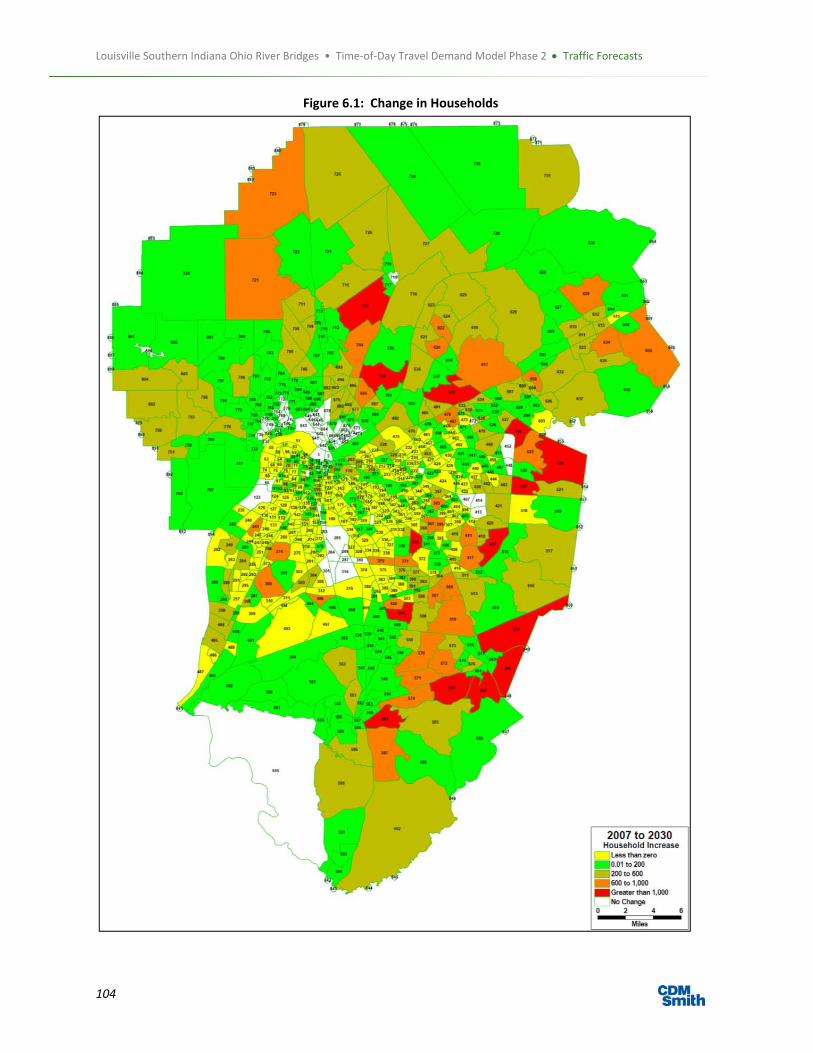
Louisville Southern Indiana Ohio River Bridges • Time‐of‐Day Travel Demand Model Phase 2 Traffic Forecasts
104
Figure 6.1: Change in Households

Louisville Southern Indiana Ohio River Bridges • Time‐of‐Day Travel Demand Model Phase 2 Traffic Forecasts
105
Figure 6.2: Change in Employment

Louisville Southern Indiana Ohio River Bridges • Time‐of‐Day Travel Demand Model Phase 2 Traffic Forecasts
106
6.2 External Forecasts An important component of the future year forecasts is the growth at the external stations. To develop the
external forecasts for the LSIORB model, CDM Smith researched available historical data at each external
station and then developed a regression based 2030 forecast volume. Observed average daily traffic (ADT)
counts were obtained from the Kentucky Transportation Cabinet and the Indiana Departments of
Transportations as well as field counts conducted by The Traffic Group, Inc. for each of the 48 external
stations within the LSIORB travel demand model. This historical data from 1990 to 2010 were used to
forecast year 2030 ADT. The distribution of traffic into external through vs. external‐internal and auto vs.
truck are based on the base year distribution assumptions.
Table 6.3 reports the available historic data for each external station from 1990 through 2010. Data are not
available for each year and are limited for several of the study area external stations, especially in Indiana.
Trend values were calculated for base year 2007 and forecast year 2030 in order to develop an annual
growth rate. The trend annual growth rate was then applied to observed counts used in the base year 2007
LSIORB model. As a result of limited data, for several stations, trend data was not able to be obtained
resulting in zero volume for the 2030 forecast. For these stations the “2030 KIPDA” forecast from the
KIPDA travel demand model was used as the LSIORB forecast. Similarly, for external stations US 31 and US
150 in Indiana, the trend showed negative or very low growth between 2007 and 2030. For these stations
(highlighted in dark grey) the “2030 KIPDA” forecast from the KIPDA travel demand model was used as the
LSIORB forecast.

Louisville Southern Indiana Ohio River Bridges • Time‐of‐Day Travel Demand Model Phase 2 Traffic Forecasts
107
Table 6.4 reports the resulting forecasted volumes for the 2030 LISORB model. These values are shown in
the “2030 Model” column.
All external stations increase in traffic between years 2007 and 2030 except for a slight decrease in traffic
on S Bloomington Trail Rd in Clark County, Indiana. Overall, there is a yearly 2.13% increase in ADT for the
external stations between years 2007 and 2030.
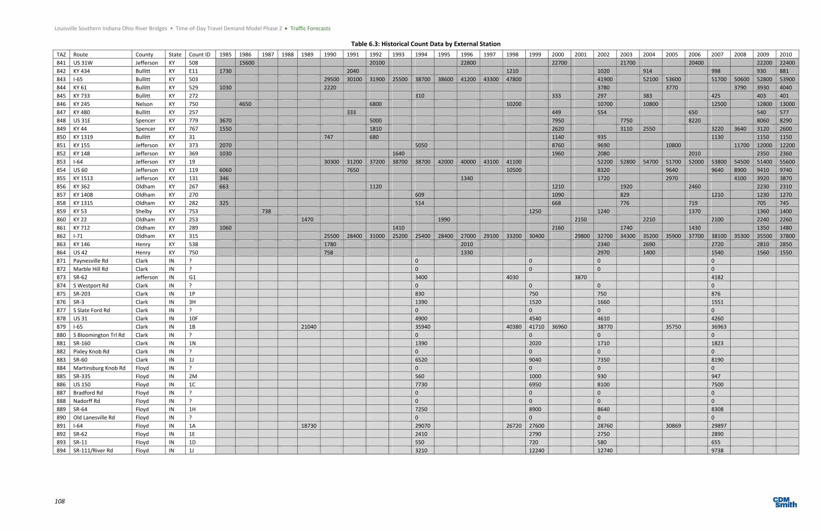
Louisville Southern Indiana Ohio River Bridges • Time‐of‐Day Travel Demand Model Phase 2 Traffic Forecasts
108
Table 6.3: Historical Count Data by External Station
TAZ Route County State Count ID 1985 1986 1987 1988 1989 1990 1991 1992 1993 1994 1995 1996 1997 1998 1999 2000 2001 2002 2003 2004 2005 2006 2007 2008 2009 2010
841 US 31W Jefferson KY 508 15600 20100 22800 22700 21700 20400 22200 22400
842 KY 434 Bullitt KY E11 1730 2040 1210 1020 914 998 930 881
843 I‐65 Bullitt KY 503 29500 30100 31900 25500 38700 38600 41200 43300 47800 41900 52100 53600 51700 50600 52800 53900
844 KY 61 Bullitt KY 529 1030 2220 3780 3770 3790 3930 4040
845 KY 733 Bullitt KY 272 310 333 297 383 425 403 401
846 KY 245 Nelson KY 750 4650 6800 10200 10700 10800 12500 12800 13000
847 KY 480 Bullitt KY 257 333 449 554 650 540 577
848 US 31E Spencer KY 779 3670 5000 7950 7750 8220 8060 8290
849 KY 44 Spencer KY 767 1550 1810 2620 3110 2550 3220 3640 3120 2600
850 KY 1319 Bullitt KY 31 747 680 1140 935 1130 1150 1150
851 KY 155 Jefferson KY 373 2070 5050 8760 9690 10800 11700 12000 12200
852 KY 148 Jefferson KY 369 1030 1640 1960 2080 2010 2350 2360
853 I‐64 Jefferson KY 19 30300 31200 37200 38700 38700 42000 40000 43100 41100 52200 52800 54700 51700 52000 53800 54500 51400 55600
854 US 60 Jefferson KY 119 6060 7650 10500 8320 9640 9640 8900 9410 9740
855 KY 1513 Jefferson KY 131 346 1340 1720 2970 4100 3920 3870
856 KY 362 Oldham KY 267 663 1120 1210 1920 2460 2230 2310
857 KY 1408 Oldham KY 270 609 1090 829 1210 1230 1270
858 KY 1315 Oldham KY 282 325 514 668 776 719 705 745
859 KY 53 Shelby KY 753 738 1250 1240 1370 1360 1400
860 KY 22 Oldham KY 253 1470 1990 2150 2210 2100 2240 2260
861 KY 712 Oldham KY 289 1060 1410 2160 1740 1430 1350 1480
862 I‐71 Oldham KY 315 25500 28400 31000 25200 25400 28400 27000 29100 33200 30400 29800 32700 34300 35200 35900 37700 38100 35300 35500 37800
863 KY 146 Henry KY 538 1780 2010 2340 2690 2720 2810 2850
864 US 42 Henry KY 750 758 1330 2970 1400 1540 1560 1550
871 Paynesville Rd Clark IN ? 0 0 0 0
872 Marble Hill Rd Clark IN ? 0 0 0 0
873 SR‐62 Jefferson IN G1 3400 4030 3870 4182
874 S Westport Rd Clark IN ? 0 0 0 0
875 SR‐203 Clark IN 1P 830 750 750 876
876 SR‐3 Clark IN 3H 1390 1520 1660 1551
877 S Slate Ford Rd Clark IN ? 0 0 0 0
878 US 31 Clark IN 10F 4900 4540 4610 4260
879 I‐65 Clark IN 1B 21040 35940 40380 41710 36960 38770 35750 36963
880 S Bloomington Trl Rd Clark IN ? 0 0 0 0
881 SR‐160 Clark IN 1N 1390 2020 1710 1823
882 Pixley Knob Rd Clark IN ? 0 0 0 0
883 SR‐60 Clark IN 1J 6520 9040 7350 8190
884 Martinsburg Knob Rd Floyd IN ? 0 0 0 0
885 SR‐335 Floyd IN 2M 560 1000 930 947
886 US 150 Floyd IN 1C 7730 6950 8100 7500
887 Bradford Rd Floyd IN ? 0 0 0 0
888 Nadorff Rd Floyd IN ? 0 0 0 0
889 SR‐64 Floyd IN 1H 7250 8900 8640 8308
890 Old Lanesville Rd Floyd IN ? 0 0 0 0
891 I‐64 Floyd IN 1A 18730 29070 26720 27600 28760 30869 29897
892 SR‐62 Floyd IN 1E 2410 2790 2750 2890
893 SR‐11 Floyd IN 1D 550 720 580 655
894 SR‐111/River Rd Floyd IN 1J 3210 12240 12740 9738

Louisville Southern Indiana Ohio River Bridges • Time‐of‐Day Travel Demand Model Phase 2 Traffic Forecasts
109
Table 6.4: Average Daily Traffic Volumes by External Station
TAZ Route County State Count ID 2007 Trend
2030 Trend
Trend Annual Growth
2007 Model 2030 Forecast
2030 KIPDA
Updated Annual Growth
2030 Model
841 US 31W Jefferson KY 508 22319 26856 0.63% 22189 25424 28276 0.63% 25424
842 KY 434 Bullitt KY E11 944 0 0.00% 998 0 2458 6.36% 2458
843 I‐65 Bullitt KY 503 52289 81451 2.42% 50618 78849 81063 2.42% 78170
844 KY 61 Bullitt KY 529 3863 6441 2.62% 5723 9166 5516 2.62% 9238
845 KY 733 Bullitt KY 272 389 559 1.90% 425 611 558 1.90% 611
846 KY 245 Nelson KY 750 12268 20265 2.77% 11162 18266 20898 2.77% 18266
847 KY 480 Bullitt KY 257 571 880 2.35% 2237 3448 1057 2.35% 3374
848 US 31E Spencer KY 779 8196 12603 2.23% 7240 10948 13059 2.23% 10948
849 KY 44 Spencer KY 767 3033 4605 2.27% 3223 4908 5127 2.27% 4908
850 KY 1319 Bullitt KY 31 1118 1647 2.05% 1134 1670 2238 2.05% 1680
851 KY 155 Jefferson KY 373 11316 21082 3.78% 11652 21781 21842 3.78% 21781
852 KY 148 Jefferson KY 369 2231 3375 2.09% 2352 3481 3323 2.09% 3481
853 I‐64 Jefferson KY 19 53972 81443 2.21% 51360 77502 72195 2.21% 76017
854 US 60 Jefferson KY 119 9503 12217 1.02% 8895 10983 11094 1.02% 10757
855 KY 1531 Jefferson KY 131 3368 6958 5.17% 4096 8964 6667 5.17% 8964
856 KY 362 Oldham KY 267 2148 3779 3.41% 2234 3987 4211 3.41% 3987
857 KY 1408 Oldham KY 270 1161 2043 3.30% 1211 2130 2070 3.30% 2130
858 KY 1315 Oldham KY 282 736 1121 2.08% 705 1043 1278 2.08% 1043
859 KY 53 Shelby KY 753 1362 2005 2.06% 1696 2424 2877 2.06% 2424
860 KY 22 Oldham KY 253 2214 2942 1.43% 2104 2796 3719 1.43% 2691
861 KY 712 Oldham KY 289 1591 1864 0.27% 1348 1431 2274 0.27% 1431
862 I‐71 Oldham KY 315 36065 50095 1.69% 35450 49241 48168 1.69% 49615
863 KY 146 Henry KY 538 2709 4019 2.10% 2715 4027 4054 2.10% 4054
864 US 42 Henry KY 750 1731 2479 1.88% 1543 2210 2188 1.88% 1967
871 Paynesville Rd Clark IN ? 0 0 0.00% 100 0 368 11.65% 368
872 Marble Hill Rd Clark IN ? 0 0 0.00% 369 0 971 7.09% 971
873 SR‐62 Jefferson IN G1 4235 5432 1.23% 4182 5364 3612 1.23% 5364
874 S Westport Rd Clark IN ? 0 0 0.00% 239 0 417 3.24% 417
875 SR‐203 Clark IN 1P 823 901 0.41% 876 958 1177 0.41% 958
876 SR‐3 Clark IN 3H 1622 1947 0.87% 1667 2001 2675 0.87% 2001
877 S Slate Ford Rd Clark IN ? 0 0 0.00% 270 0 278 0.13% 278
878 US 31 Clark IN 10F 4281 3233 ‐1.06% 4750 3587 5342 0.54% 5342
879 I‐65 Clark IN 1B 41241 56977 2.48% 36962 58061 64783 2.48% 57303
880 S Bloomington Trl Rd Clark IN ? 0 0 0.00% 541 0 417 ‐1.00% 417
881 SR‐160 Clark IN 1N 1907 2515 1.38% 1946 2565 2567 1.38% 2565
882 Pixley Knob Rd Clark IN ? 0 0 0.00% 135 0 249 3.67% 249
883 SR‐60 Clark IN 1J 8383 10533 1.12% 8649 10867 9809 1.12% 10867
884 Martinsburg Knob Rd Floyd IN ? 0 0 0.00% 367 0 695 3.89% 695
885 SR‐335 Floyd IN 2M 1035 1658 2.62% 1260 2018 2423 2.62% 2018
886 US 150 Floyd IN 1C 7587 7646 0.03% 7272 7329 10271 1.79% 10271
887 Bradford Rd Floyd IN ? 0 0 0.00% 0 0 687 0.00% 687
888 Nadorff Rd Floyd IN ? 0 0 0.00% 0 0 417 0.00% 417
889 SR‐64 Floyd IN 1H 8748 10425 0.83% 8092 9643 12239 0.83% 9643
890 Old Lanesville Rd Floyd IN ? 0 0 0.00% 0 0 973 0.00% 973
891 I‐64 Floyd IN 1A 31524 43660 2.36% 29896 46150 48663 2.36% 45713
892 SR‐62 Floyd IN 1E 2933 3724 1.17% 2651 3366 3908 1.17% 3366
893 SR‐11 Floyd IN 1D 661 783 0.80% 617 731 967 0.80% 731
894 SR‐111/River Rd Floyd IN 1J 12636 23795 3.84% 11589 21824 17400 3.84% 21824

Louisville Southern Indiana Ohio River Bridges • Time‐of‐Day Travel Demand Model Phase 2 Traffic Forecasts
110
These ADT percent increases are consistent with the truck growth between 2007 and 2030. The truck
percent of total ADT is held constant between the base year and the forecast year. Similarly, the split
between EE and EI trips are held constant between the base and forecast years. The percent trucks of total
ADT is shown in Table 6.5 along with the corresponding annual growth of truck traffic. Interstate 65 in
Clark County, IN has the highest percentage of trucks at 44% of the total ADT. Similarly, Interstate 71 in
Oldham County, KY has a high truck percentage of 41% of the total ADT.
Table 6.5: LSIORB Model Truck Percentages and Growth
Route 2007 Count
2007 Model
2030 Model
Percent Trucks
Model Growth/Yr
I‐65 KY 18,111 19,282 28,213 36% 1.67%
I‐64 KY 9,302 10,108 14,038 18% 1.44%
I‐71 KY 14,504 15,473 20,146 41% 1.15%
I‐65 IN 16,263 16,273 25,547 44% 1.98%
I‐64 IN 10,168 9,300 14,307 31% 1.89%
Table 6.6 shows the Freight Analysis Framework (FAF) version 3 data of truck percentage of daily traffic
and truck annual growth for the external stations. This table shows a higher growth in traffic than the
historical counts, especially for the Indiana counts.
Table 6.6: Freight Analysis Framework Truck Percentages and Growth (Source: FAF3, 2040 Forecast)
Route 2007 FAF 2040 FAF FAF 2040 % Trucks
FAF Growth/Yr
I‐65 KY 21804 39035 49% 1.78%
I‐64 KY 7960 12524 15% 1.38%
I‐71 KY 13120 22574 39% 1.66%
I‐65 IN 11705 21352 31% 1.84%
I‐64 IN 5852 9355 20% 1.43%
The truck growth comparison between the FAF3 data and the model data shows that compared to the FAF
data, the model closely reflects truck percentage of total ADT for I‐64 and I‐65 in Kentucky and I‐65 in
Indiana. The model under‐estimates the I‐71 truck percentage and over‐estimates the I‐64 truck
percentages in Indiana compared to the FAF data. For the truck percent of total ADT the model tends to
over‐estimate interstate truck percentage of traffic in Indiana and under‐estimate truck percentage on I‐65
in Kentucky.

Appendix A – KYTC, CTS, and KIPDA Comments
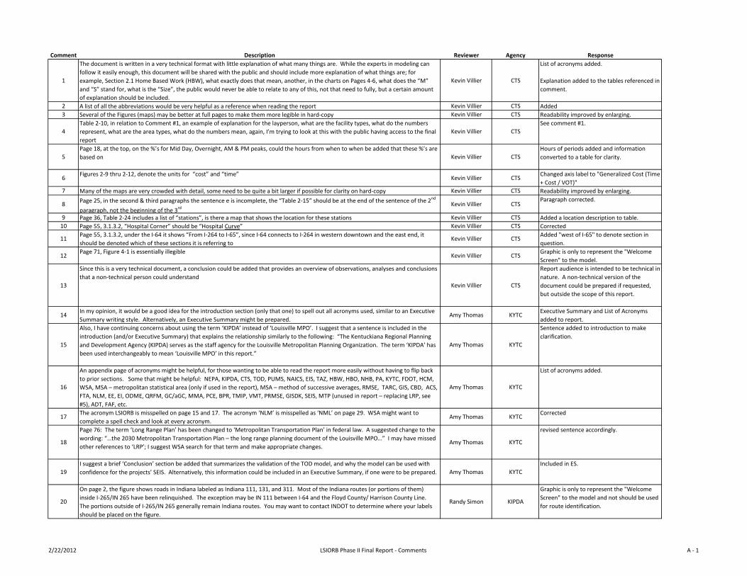
Comment Description Reviewer Agency Response
1
The document is written in a very technical format with little explanation of what many things are. While the experts in modeling can
follow it easily enough, this document will be shared with the public and should include more explanation of what things are; for
example, Section 2.1 Home Based Work (HBW), what exactly does that mean, another, in the charts on Pages 4-6, what does the “M”
and “S” stand for, what is the “Size”, the public would never be able to relate to any of this, not that need to fully, but a certain amount
of explanation should be included.
Kevin Villier CTS
List of acronyms added.
Explanation added to the tables referenced in
comment.
2 A list of all the abbreviations would be very helpful as a reference when reading the report Kevin Villier CTS Added
3 Several of the Figures (maps) may be better at full pages to make them more legible in hard-copy Kevin Villier CTS Readability improved by enlarging.
4
Table 2-10, in relation to Comment #1, an example of explanation for the layperson, what are the facility types, what do the numbers
represent, what are the area types, what do the numbers mean, again, I’m trying to look at this with the public having access to the final
report
Kevin Villier CTS
See comment #1.
5
Page 18, at the top, on the %’s for Mid Day, Overnight, AM & PM peaks, could the hours from when to when be added that these %’s are
based on Kevin Villier CTS
Hours of periods added and information
converted to a table for clarity.
6Figures 2-9 thru 2-12, denote the units for “cost” and “time”
Kevin Villier CTSChanged axis label to "Generalized Cost (Time
+ Cost / VOT)"
7 Many of the maps are very crowded with detail, some need to be quite a bit larger if possible for clarity on hard-copy Kevin Villier CTS Readability improved by enlarging.
8Page 25, in the second & third paragraphs the sentence e is incomplete, the “Table 2-15” should be at the end of the sentence of the 2nd
paragraph, not the beginning of the 3rdKevin Villier CTS
Paragraph corrected.
9 Page 36, Table 2-24 includes a list of “stations”, is there a map that shows the location for these stations Kevin Villier CTS Added a location description to table.
10 Page 55, 3.1.3.2, “Hospital Corner” should be “Hospital Curve” Kevin Villier CTS Corrected
11Page 55, 3.1.3.2, under the I-64 it shows “From I-264 to I-65”, since I-64 connects to I-264 in western downtown and the east end, it
should be denoted which of these sections it is referring toKevin Villier CTS
Added "west of I-65" to denote section in
question.
12Page 71, Figure 4-1 is essentially illegible
Kevin Villier CTSGraphic is only to represent the "Welcome
Screen" to the model.
13
Since this is a very technical document, a conclusion could be added that provides an overview of observations, analyses and conclusions
that a non-technical person could understand
Kevin Villier CTS
Report audience is intended to be technical in
nature. A non-technical version of the
document could be prepared if requested,
but outside the scope of this report.
14In my opinion, it would be a good idea for the introduction section (only that one) to spell out all acronyms used, similar to an Executive
Summary writing style. Alternatively, an Executive Summary might be prepared. Amy Thomas KYTC
Executive Summary and List of Acronyms
added to report.
15
Also, I have continuing concerns about using the term ‘KIPDA’ instead of ‘Louisville MPO’. I suggest that a sentence is included in the
introduction (and/or Executive Summary) that explains the relationship similarly to the following: “The Kentuckiana Regional Planning
and Development Agency (KIPDA) serves as the staff agency for the Louisville Metropolitan Planning Organization. The term ‘KIPDA’ has
been used interchangeably to mean ‘Louisville MPO’ in this report.”
Amy Thomas KYTC
Sentence added to introduction to make
clarification.
16
An appendix page of acronyms might be helpful, for those wanting to be able to read the report more easily without having to flip back
to prior sections. Some that might be helpful: NEPA, KIPDA, CTS, TOD, PUMS, NAICS, EIS, TAZ, HBW, HBO, NHB, PA, KYTC, FDOT, HCM,
WSA, MSA – metropolitan statistical area (only if used in the report), MSA – method of successive averages, RMSE, TARC, GIS, CBD, ACS,
FTA, NLM, EE, EI, ODME, QRFM, GC/aGC, MMA, PCE, BPR, TMIP, VMT, PRMSE, GISDK, SEIS, MTP (unused in report – replacing LRP, see
#5), ADT, FAF, etc.
Amy Thomas KYTC
List of acronyms added.
17The acronym LSIORB is misspelled on page 15 and 17. The acronym ‘NLM’ is misspelled as ‘NML’ on page 29. WSA might want to
complete a spell check and look at every acronym.Amy Thomas KYTC
Corrected
18
Page 76: The term ‘Long Range Plan’ has been changed to ‘Metropolitan Transportation Plan’ in federal law. A suggested change to the
wording: “…the 2030 Metropolitan Transportation Plan – the long range planning document of the Louisville MPO…” I may have missed
other references to ‘LRP’; I suggest WSA search for that term and make appropriate changes.Amy Thomas KYTC
revised sentence accordingly.
19
I suggest a brief ‘Conclusion’ section be added that summarizes the validation of the TOD model, and why the model can be used with
confidence for the projects’ SEIS. Alternatively, this information could be included in an Executive Summary, if one were to be prepared. Amy Thomas KYTC
Included in ES.
20
On page 2, the figure shows roads in Indiana labeled as Indiana 111, 131, and 311. Most of the Indiana routes (or portions of them)
inside I-265/IN 265 have been relinquished. The exception may be IN 111 between I-64 and the Floyd County/ Harrison County Line.
The portions outside of I-265/IN 265 generally remain Indiana routes. You may want to contact INDOT to determine where your labels
should be placed on the figure.
Randy Simon KIPDA
Graphic is only to represent the "Welcome
Screen" to the model and not should be used
for route identification.
2/22/2012 LSIORB Phase II Final Report - Comments A - 1
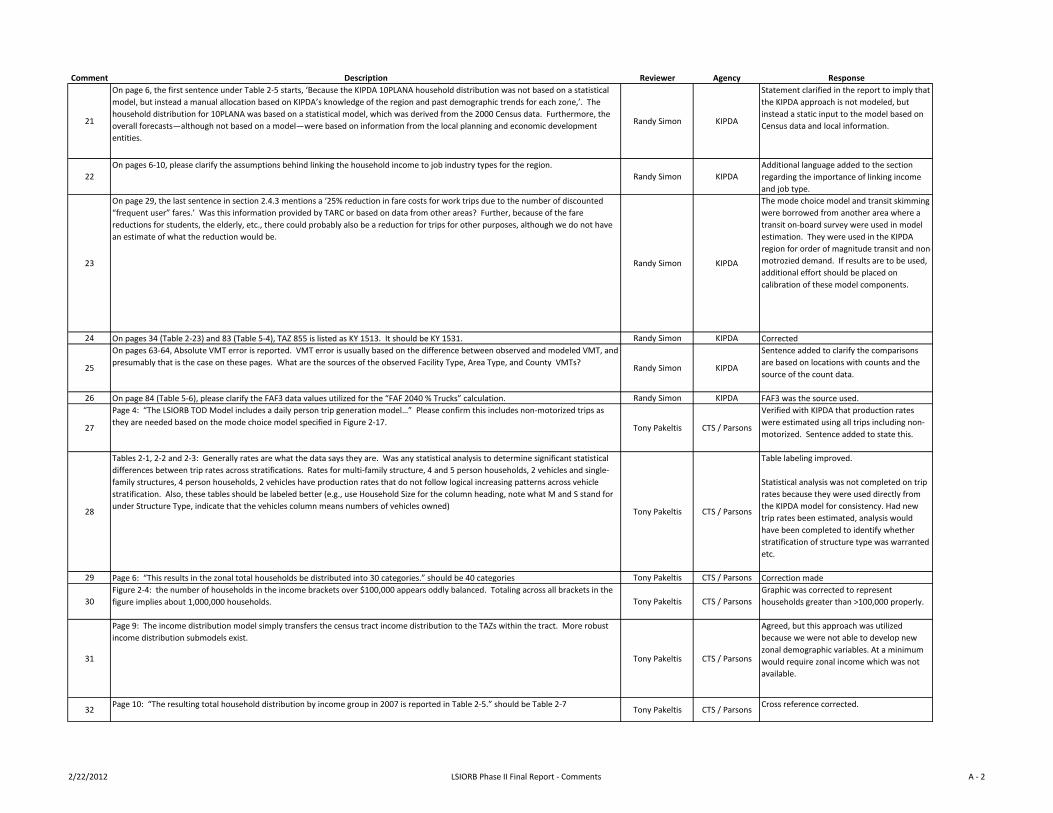
Comment Description Reviewer Agency Response
21
On page 6, the first sentence under Table 2-5 starts, ‘Because the KIPDA 10PLANA household distribution was not based on a statistical
model, but instead a manual allocation based on KIPDA’s knowledge of the region and past demographic trends for each zone,’. The
household distribution for 10PLANA was based on a statistical model, which was derived from the 2000 Census data. Furthermore, the
overall forecasts—although not based on a model—were based on information from the local planning and economic development
entities.
Randy Simon KIPDA
Statement clarified in the report to imply that
the KIPDA approach is not modeled, but
instead a static input to the model based on
Census data and local information.
22
On pages 6-10, please clarify the assumptions behind linking the household income to job industry types for the region.
Randy Simon KIPDA
Additional language added to the section
regarding the importance of linking income
and job type.
23
On page 29, the last sentence in section 2.4.3 mentions a ‘25% reduction in fare costs for work trips due to the number of discounted
“frequent user” fares.’ Was this information provided by TARC or based on data from other areas? Further, because of the fare
reductions for students, the elderly, etc., there could probably also be a reduction for trips for other purposes, although we do not have
an estimate of what the reduction would be.
Randy Simon KIPDA
The mode choice model and transit skimming
were borrowed from another area where a
transit on-board survey were used in model
estimation. They were used in the KIPDA
region for order of magnitude transit and non-
motrozied demand. If results are to be used,
additional effort should be placed on
calibration of these model components.
24 On pages 34 (Table 2-23) and 83 (Table 5-4), TAZ 855 is listed as KY 1513. It should be KY 1531. Randy Simon KIPDA Corrected
25
On pages 63-64, Absolute VMT error is reported. VMT error is usually based on the difference between observed and modeled VMT, and
presumably that is the case on these pages. What are the sources of the observed Facility Type, Area Type, and County VMTs?Randy Simon KIPDA
Sentence added to clarify the comparisons
are based on locations with counts and the
source of the count data.
26 On page 84 (Table 5-6), please clarify the FAF3 data values utilized for the “FAF 2040 % Trucks” calculation. Randy Simon KIPDA FAF3 was the source used.
27
Page 4: “The LSIORB TOD Model includes a daily person trip generation model…” Please confirm this includes non-motorized trips as
they are needed based on the mode choice model specified in Figure 2-17.Tony Pakeltis CTS / Parsons
Verified with KIPDA that production rates
were estimated using all trips including non-
motorized. Sentence added to state this.
28
Tables 2-1, 2-2 and 2-3: Generally rates are what the data says they are. Was any statistical analysis to determine significant statistical
differences between trip rates across stratifications. Rates for multi-family structure, 4 and 5 person households, 2 vehicles and single-
family structures, 4 person households, 2 vehicles have production rates that do not follow logical increasing patterns across vehicle
stratification. Also, these tables should be labeled better (e.g., use Household Size for the column heading, note what M and S stand for
under Structure Type, indicate that the vehicles column means numbers of vehicles owned)Tony Pakeltis CTS / Parsons
Table labeling improved.
Statistical analysis was not completed on trip
rates because they were used directly from
the KIPDA model for consistency. Had new
trip rates been estimated, analysis would
have been completed to identify whether
stratification of structure type was warranted
etc.
29 Page 6: “This results in the zonal total households be distributed into 30 categories.” should be 40 categories Tony Pakeltis CTS / Parsons Correction made
30
Figure 2-4: the number of households in the income brackets over $100,000 appears oddly balanced. Totaling across all brackets in the
figure implies about 1,000,000 households. Tony Pakeltis CTS / Parsons
Graphic was corrected to represent
households greater than >100,000 properly.
31
Page 9: The income distribution model simply transfers the census tract income distribution to the TAZs within the tract. More robust
income distribution submodels exist.
Tony Pakeltis CTS / Parsons
Agreed, but this approach was utilized
because we were not able to develop new
zonal demographic variables. At a minimum
would require zonal income which was not
available.
32Page 10: “The resulting total household distribution by income group in 2007 is reported in Table 2-5.” should be Table 2-7
Tony Pakeltis CTS / ParsonsCross reference corrected.
2/22/2012 LSIORB Phase II Final Report - Comments A - 2

Comment Description Reviewer Agency Response
33
Table 2-7: As reported total households across the three income groups sum to 417638.9. This does not match the total reported in
Table 2-5 or 2-6 Tony Pakeltis CTS / Parsons
Table 2.7 corrected to match previous tables.
Calculation error in table summary, model
data is correct.
34 Page 15: Typo in the second to last line. LSIROB should be LSIORB Tony Pakeltis CTS / Parsons See #17
35
Table 2-10: There should be an explanation of the facility type and area type codes.
Tony Pakeltis CTS / Parsons
Note added to table with a brief description
of codes and reference to Phase I Report.
36 Page 17: Typo in the second line. LSIROB should be LSIORB Tony Pakeltis CTS / Parsons See #17
37Table 2-11: What is the source of information or data to justify using the indicated values of time and operating cost? Value of time is
equivalent to $12.60/hour and $33.00/hour for autos and trucks respectively.Tony Pakeltis CTS / Parsons
Added a description of the source and
rationale.
38Page 19: “This process was completed until the average values from the survey were replicated within an acceptable tolerance.” What
was the acceptable tolerance?Tony Pakeltis CTS / Parsons
Sentence modified to include converge
tolerance used.
39Figures 2-9, 2-10 and 2-11: need to show some calibration statistic such as the coincidence ratio. Curves appear to match observed.
Tony Pakeltis CTS / ParsonsCoincidence ratio was added (all purposes
greater than 0.8)
40Page 21: “HBW has a higher willingness to travel as seen in the shallow slope of the curve as compared to HBW and NHB that fall off
quickly.” should be …as compared to HBO and NHB.Tony Pakeltis CTS / Parsons
Corrected
41
Page 23: “The model reaches the 0.1 RMSE threshold at iteration six but becomes fairly stable starting at iteration four and little benefit
is obtained after the fourth iteration in the 2007 model. Thus, iterations after the fourth may not warrant the additional time sacrificed
for the minimal convergence improvements.” This may be true when analyzing daily or peak period output since the convergence is
based off of an average of the AM and PM peak period travel times (for HBW). However the model may still have larger than acceptable
iteration to iteration variance within a peak hour assignment. More iterations may be warranted when focusing on peak hour results. Tony Pakeltis CTS / Parsons
Agreed that in forecast application, additional
iterations of the feedback process should be
completed. An analysis was completed of the
different volumes between iteration of
feedback and very little difference was found
after the 3rd iteration which is consistent
with the literature.
42 Page 23: Third paragraph: replace LSIROB with LSIORB Tony Pakeltis CTS / Parsons Corrected
43Page 26: “GIS procedures were used to connect the centroid nodes of all zones fully or partially within one third mile of any bus stop.
Tony Pakeltis CTS / ParsonsNo comment raised.
44
Page 28: ”Additionally, transit walk access times were developed based on a three mile per hour speed assumption and a maximum
walk time of ten minutes to transit service.” This equates to ½ mile maximum walk distance. It seems possible that a TAZ could be
outside the 1/3 mile buffer used to create walk access links but still have a centroid within ½ mile walk distance.
Tony Pakeltis CTS / Parsons
Yes, that could be possible. The first rule was
to check if the zone boundary is within a third
of a mile to the transit stop. This first rule
governs because it is assumed that if the zone
boundary is not within a third of a mile to the
stop then most likely there would not be
direct walk access to the stop from that zone.
45
Page 28: “Transit markets were specified in the LSIORB model to develop transit potential trips by household type (zero car households
and one or more car households) and by access to transit (drive access and walk access) for each trip purpose.” How are these transit
markets used in the model?
Tony Pakeltis CTS / Parsons
There are different logit models applied for
each transit market in mode choice
46
Section 2.4.3: What are the transit settings, parameters and weights used in path building? They should be consistent with parameters
used in mode choice. Tony Pakeltis CTS / Parsons
The same parameters used in transit path
building settings and resulting skims are used
in mode choice.
47
Page 31: “…and the number of transfers have a negative effect on the utility equation and the CBD or employment density dummy
variable has a positive effect.” Some professionals have argued against the use of geographic based coefficients (i.e. the CDB dummy
variable). Tony Pakeltis CTS / Parsons
This point may be valid. However, the
methodology assumed characteristics from
similar areas where the CBD attracts more
transit trips than other area types, especially
for HBW trips.
48
Table 2-20: No mode constants are listed in the table
Tony Pakeltis CTS / Parsons
Additional table added to report for mode
constants by market segment and purpose.
2/22/2012 LSIORB Phase II Final Report - Comments A - 3

Comment Description Reviewer Agency Response
49
Page 32: “…model implied value of time should be in the range average income /4 to average income /3.” What are the average
incomes and what are the models implied values of time?
Tony Pakeltis CTS / Parsons
The VOT assumptions used in the model are
consistent between all steps (trip
distribution, mode choice and traffic
assignment). See note # 23 above for more
information about source of model
parameters.
50
Table 2-20: The cost coefficients for Work and Other trips give a higher value of time to Other trips ($12.50/hr versus $6.52/hr).
Typically, Work trips would be expected to have a higher value of time.
Tony Pakeltis CTS / Parsons
The cost parameter coefficients for work and
other in the NLM of Mode Choice are
borrowed as described in the documentation.
Local surveys were not used for calibration of
the model. The model was validated to
Journey-to-Work percent mode shares and
transit trip by purpose data borrowed from
similar areas with adjustment of the mode
constants as is typical practice. When Ken
Cervenka, FTA reviewed the source model
(CHATS), he also acknowledges the lower
HBW VOT. He states in an email “This doesn’t
mean you are wrong, but I am curious as to
whether you have seen this type of VOT
difference amongst purposes from other
studies” beyond the CHATS On-Board study.
51
Page 38: “The issue of the decreasing expansion rate for station 2N (attraction) as well as the imbalance of the attraction trip totals
(Table 2) to the matched plates (Table 1) results in some uncertainty with the attraction trips.” What are Tables 2 and 1? Are they
possibly 2-28 and 2-27 respectively?
Tony Pakeltis CTS / Parsons
Corrected
52Page 38: “The TransCAD modeling software was used to fratar the raw survey data of EE trips (Table 4) with the sum of the expanded EE
productions (Table 2-28) for passenger vehicles.” What is Table 4?Tony Pakeltis CTS / Parsons
Corrected
53
Page 51: “The graphical user interface allows the use of unique values of time by income group for the auto trips, and unique values of
time for light truck and heavy truck flows.” What values of time have been proposed for use with the forecasts?
Tony Pakeltis CTS / Parsons
For the SEIS the VOT and VOC used in
validation were applied for the forecast since
constant dollars were assumed in the
forecast. The GUI was created to allow
flexibility for future applications. (Table 2-11)
54
Page 54, Table 3-2: “The K-factors were adjusted based on improving the JTW comparison and the screen line validation while
maintaining reasonable values.” What are reasonable values? A more rigorous standard for using K-factors includes using them
sparingly and limited the range from 0.5 to 2.0 to ensure that they did not dominate the calibrated friction factors. The use of very large
(or small) K-factors can have the tendency to fix the distribution and make it relatively insensitive to changes in the transportation
network. Tony Pakeltis CTS / Parsons
In principle agree, but given the high
proportion of employment in Jefferson
County as compared to the rest of the region
and geographic barriers (Ohio River), they
may be warranted in this case. Future
enhancements to the trip generation model
(rates by district) may reduce the
dependence on k-factors.
55
Figure 3-1: An overall goal for percent RMSE should be less than 30.
Tony Pakeltis CTS / Parsons
An overall goal of a percent RMSE less than
30 is desirable, but it is not a "pass / fail"
criteria in the literature. Further, by volume
group, the LSIORB TOD Model is well under
the TMIP Criteria (Figure 3-5).
2/22/2012 LSIORB Phase II Final Report - Comments A - 4

Comment Description Reviewer Agency Response
56Page 62: “Figure 3-2 demonstrates that for all facility type groups, the LSIORB TOD Model is below the established criteria.” This is true
except for the One Way class shown.Tony Pakeltis CTS / Parsons
Amended sentence to reflect one-way streets
exceed by 2%.
57Figures 3-2, 3-3, 3-4: It would be helpful to see how many count locations were available for each classification grouping.
Tony Pakeltis CTS / ParsonsThe distribution of 1265 counts is shown in a
new table.
58
Figure 3-6: Clark Memorial Bridge volumes are considerably lower than counts. Is this a direct trade-off with the volumes on I-65 which
closely match the counts?Tony Pakeltis CTS / Parsons
The trade off is based on a) the validation on I-
65, and the relative distribution of traffic
under forecast conditions when applying the
model.
59Table 3-7: Typically, it is desirable to match screenline crossings to within ±15 percent. It would also be helpful to see how many count
locations were used to define each screenline.Tony Pakeltis CTS / Parsons
See #57
60
Section 3.2.3: It appears as the model has forecast too much traffic during the peak periods and to little in the off-peak periods. Again it
would be helpful to see how many count locations were in each facility group by period.
Tony Pakeltis CTS / Parsons
See #57
Further, the model was validated to AADT,
and period validation was for order of
magnitude check only. This is a typical
comparison based on the reporting time of
trip departure vs count distributions in TOD
Models.
61
You’ve referenced the 1997 validation manual, but not the 2nd edition dated September 24, 2010. Please reference the newer manual
with additional documentation of the processes and results. Scott Thomson KYTC
Changed reference to 2nd edition, but
sections used in the LSIORB Validation are
unchanged between 1st and 2nd version.
62
2.3.1 Friction Factor Calibration….What was the range of values? Friction Factors can make the model insensitive to changes. Please
document the range and frequency of values using a visual histogram. Scott Thomson KYTC
The friction factors are shown in Figure 4.12
in the report.
63
2.3.2.2 Convergence Criteria… You mention 0.1 RMSE as the threshold, but we’re more accustomed to it as a numerical value. Is this the
same as .001? Recent Caliper white papers have reference values of .0001 or better(smaller).
Scott Thomson KYTC
The threshold applied was based on a review
of the literature and our experience with
feeedback models in Austin, TX. The model is
achieving stability based on the converge
calculation and a comparison of volumes by
period after iteration #3.
64
2.5.1 Data Collection This and the following sections describe Stations as 1N, 1S, etc. however, no figure is provided or referenced.
Please provide a map that highlights the stations and the nomenclature used in the tables. (so the previous Phase 1 document isn’t a
required reference.
Scott Thomson KYTC
Map added.
65
3.2 Validation Results Figure 3-1 demonstrates a trend in the overall error (ie. RMSE) but doesn’t provide an idea of the models overall
performance when compared to data. Please include a figure where count vs flow is plotted relating to ADT’s. Since this is a TOD model,
can the hourly counts of the results be displayed in a similar manner? Scott Thomson KYTC
Provided a map of the daily validation results
showing under and over assigned. Not
appropriate to show peak validation since
model validated to daily conditions.
66
3.2.2 Daily Assignment Validation FHWA criteria is mentioned. Please document the methodology used to establish the values. The link
below includes a table, but doesn’t appear to correlate with the ‘Criteria’ line in figure 3-5
http://tmip.fhwa.dot.gov/resources/clearinghouse/docs/FHWA-HEP-10-042/ch9.htm Figure 3-2 and 3-3 do not label the Y-axis (what are
the units of VMT error?)
Scott Thomson KYTC
Corrected the curve in the figure represent
the correct curve from the TMIP Guide.
67Table 3-9 VMT Error by Facility Group by Period. Convert the Facility Group labels from numbers (10,20,30,etc) to match the Facility
Group labels used on figure 3-2Scott Thomson KYTC
Change made.
2/22/2012 LSIORB Phase II Final Report - Comments A - 5

KENTUCKYTRANSPORTATION
CABINET
Prepared by: