Empirical Analysis of Economic Institutions Discussion Paper Series

No.14

Dept, R&D Investment and Technological Progress: A Panel Study of Japanese Manufacturing Firms in the 90s

Kazuo Ogawa

December 2003

This discussion paper series reports research for the project entitled “Empirical Analysis of Economic Institutions”, supported by Grants-in-Aid for Scientific Research of the Ministry of Education and Technology.

December 2003

Debt, R&D Investment and Technological Progress: A Panel Study of Japanese Manufacturing Firms in the 90s*

Kazuo Ogawa

Institute of Social and Economic Research, Osaka University

* I am grateful to Kazuyuki Suzuki, Yosuke Takeda, Fukujyu Yamazaki and the participants of the

seminar at Sophia University for extremely helpful comments and suggestions. I would like to thank

Junmin Wan for excellent research assistance. This research was partially supported by

Grants-in-Aid for Scientific Research 12124207 of the Ministry of Education. Any remaining errors

are the sole responsibility of the author.

Abstract

Based on a panel data set of Japanese manufacturing firms in research-intensive

industries, we investigate quantitatively the extent to which debt outstandings in the 90s affected the firm’s R&D activities. We find that massive debt outstandings had significantly negative effect on R&D investment in the 90s. We also find that investment on R&D was closely linked to the firm-level total factor productivity growth in the 90s. Thus it is concluded that massive debt outstandings in the 90s lowered the firm-level total factor productivity growth rate by withering R&D activities. JEL Classification Number: D21,D24 and O32 Keywords: R&D investment, Debt, Total factor productivity Correspondence to: Institute of Social and Economic Research, Osaka University, 6-1 Mihogaoka, Ibaraki, Osaka, 567-0047 JAPAN Tel: +81- 6- 6879-8570 Fax: +81- 6-6878-2766 E-mail: ogawa@iser.osaka-u.ac.jp

1

1. Introduction

Consensus is not yet reached on the causes to bring long stagnancy to the

Japanese economy in the 90s. The supply-siders argue that stagnancy is mainly due to

supply factors such as inefficiencies of the production sector as well as banking sector

suffering from massive bad loans and warn that the growth potential of the Japanese

economy is withering. For example, Hayashi and Prescott(2002) demonstrate, based on

the standard growth model, that decline of the total factor productivity(abbreviated as

TFP) growth rate and shortened working hour is responsible for the stagnancy of the

Japanese economy. Convincing as their argument is, they are silent on why the TFP

growth rate suddenly dropped in the 90s.

We shed light on this aspect empirically. Recently an attempt is made to find the

mechanism why the aggregate or industry-level TFP growth rate declined in the 90s.

Nishimura et al. (2003) and Fukao and Kwon(2003) argue that efficient firms exit from

the market, while inefficient firms remain in the market, which leads to the decline of

the aggregate TFP growth rate in the middle of the 90s. We are interested in the

firm-level TFP growth and its association with the firm’s R&D activities in the 90s.

Based on a panel data of Japanese manufacturing firms, we examine the R&D

investment of the firm and how they are linked to the firm-level TFP growth rate. Our

panel data set is composed of listed firms in chemicals, machinery, electrical machinery,

equipment and supplies, transport equipment and precision instrument industries all of

which are quite research-intensive. Specifically we investigate the extent to which debt

outstandings of the firm and bad loans burdened on banks affected the R&D investment

of the firm and subsequently the TFP growth rate. To do so, comparison is made

between the R&D activities of the firm in the late 80s and the late 90s. The former

period is the midst of bubble booms, while the latter period is characterized by heavy

debt overhang in the corporate sector and mounting bad loans in the banking sector.

We preview our main findings. The ratio of debt to total assets has significantly

negative effect on R&D investment in the late 90s, while the effect of debt-asset ratio on

R&D investment is insignificant in the late 80s on the whole. Therefore it is massive

debt outstandings of the firm that inactivated R&D activities in the late 90s. We also

2

find that the TFP growth rate is positively linked to R&D investment, which implies

that debt overhang in the 90s is responsible for lowering the firm-level TFP growth rate.

Furthermore, it is found that larger dispersion of debt-asset ratio across firms leads to

more dispersed distribution of R&D investment in the 90s.

The paper is organized as follows. The next section shows salient characteristics

of R&D activities of the Japanese manufacturing industry as a whole as well as

individual firm in our panel data set in the 90s. Section 3 estimates the investment

function of R&D and Section 4 examines the association of investment on R&D with

the firm-level TFP growth rate. Section 5 concludes the paper.

2. Characteristics of R&D Activities and the TFP Growth of the Japanese

Manufacturing Firms in the 90s

We uncover some salient characteristics of R&D activities of the Japanese

manufacturing industry as a whole in the 90s as well as individual firms in our panel

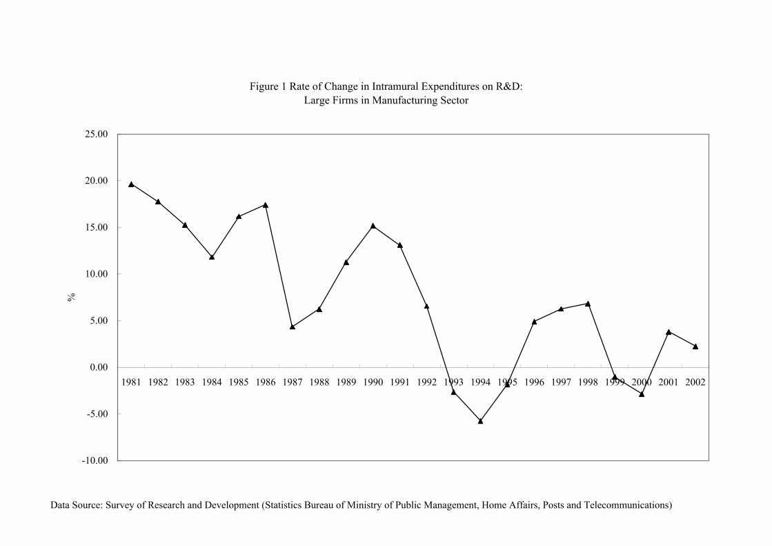
data set. First of all, R&D activities of Japanese manufacturing industry had been

stagnant in the 90s. This can be confirmed by the following three figures. Figure 1

shows the rate of change in intramural expenditures on R&D of large firms in the

manufacturing sector from 1981 to 2002. Large firms are defined as those whose equity

capital is over 1 billion yen. In the 80s the rate of change in intramural expenditures on

R&D exceeded 10 % per annum for most of the period, but it fell sharply in 1993 and

stayed low thereafter. The average annual growth rate of intramural expenditures on

R&D during 1981-1990 is 13.5 %, but it is only 2.46 % during 1991-2002. The rate of

change in persons engaged in R&D activities, shown in Figure2, also exhibits the same

tendency. The rate of change in persons engaged in R&D activities fell sharply in 1994

and hovered around zero thereafter. The average annual growth rate of persons engaged

in R&D activities during 1981-1990 is 6.27 %, while it is nearly zero (0.2 %) during

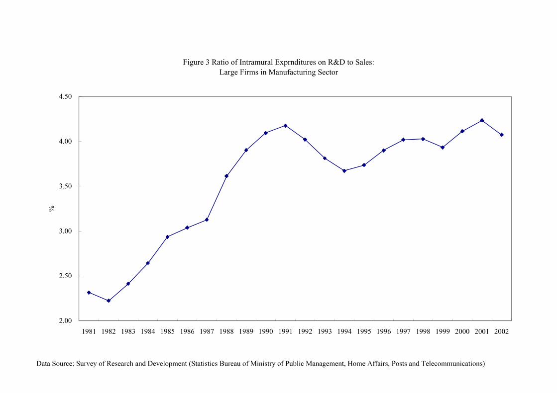
1991-2002. Reflecting low rate of change in intramural expenditures on R&D, the ratio

of intramural expenditure on R&D to sales remained stagnant in the 90s, as is shown in

Figure 3.

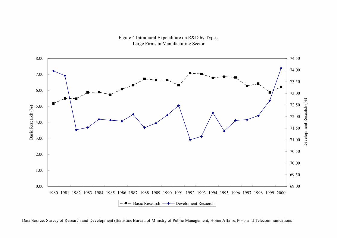
The second feature is a tilt toward development research from basic research.

3

Figure 4 shows the proportions of expenditures appropriated for basic R&D research. In

the 80s the proportion of expenditures on basic research increased steadily from 5.18 %

in 1980 to 7.07 % in 1992. However, it declined gradually in the 90s and the proportion

of development research rose steeply. The share of development research increased

from 1992 to 2000 by 3-percentage point. This might reflect myopic R&D behavior of

manufacturing firms under increasing uncertainty over the investment outcome since it

takes more time for the development research to bear fruit.

Next we characterize the R&D activities of individual firms in our panel data set.

All the firm-level data series are taken from Development Bank of Japan Corporate

Database. Our sampled firms belong to the following five industries: chemicals,

machinery, electrical machinery, equipment and supplies, transport equipment and

precision instrument. These industries are quite research-intensive in the sense that the

ratio of expenditure on R&D to sales is relatively high. The number of firms as well as

total observations for each industry is shown in Table 1. All the firms do not report the

figures of expenditures on R&D for every year, so that our panel data set is unbalanced.

Table 2 compares the averaged ratio of expenditure on R&D to sales for each industry

between the two periods: 1988-91 and 1999-2001. This ratio falls drastically in the 90s

for electrical machinery, equipment and supplies industry that is most research-intensive.

It should be noted that even the R&D activities of research-intensive firms became

stagnant in the 90s.

Now we see how the firm-level TFP growth rate has changed in the 90s. Based on

the panel data set described above, we compare the average TFP growth rates of five

industries between the late 80s and the late 90s. The TFP growth rate is calculated in

two different ways. One way is to subtract the contribution of labor input growth and

capital stock growth from the growth rate of real value-added.1 In other words, the

firm-level TFP growth rate is calculated as

( ) ( ) ( ) ( )ititLititLitit KsLsYTFP log1loglog ,, ∆−−∆−∆= (1)

where itTFP : TFP growth rate of the i-th firm in year t

4

itY : real value-added of the i-th firm in year t

itL : labor input of the i-th firm in year t

itK : capital stock of the i-th firm at the end of year t

itLs , : labor share of the i-th firm in year t

The firm-level TFP growth rate thus calculated is averaged out for each industry.

Alternative way to obtain the industry-level TFP growth rate is to estimate the

Cobb-Douglas production function of value-added type by industry with labor, capital

stock and time trend as regressors and identify the estimated coefficient of time trend as

the industry-level TFP growth rate. The production function is estimated by either fixed

effects model or variance components model, depending on the Hausman test statistics.

The estimated TFP growth rates for the two periods: 1988-91 and 1999-2001 are

shown in Table 3. The TFP growth rates constructed from the firm-level TFP growth

rate by the first method are given in the first column (1988-91) and third column

(1999-2001). Unexpectedly the TFP growth rates are higher in the late 90s except for

chemicals and precision instrument industries. However, as for the statistical

significance of the estimates, the average TFP growth rate is significantly positive for

all the industries in the late 80s, while the average TFP growth rate is significantly

positive only for electrical machinery, equipment and supplies and transport equipment.

This reflects higher standard deviation of the TFP growth rate in the late 90s. It implies

that the distribution of the firm-level TFP growth rate is more dispersed in the late 90s

than in the late 80s. Statistically the average TFP growth rate is higher for electrical

machinery, equipment and supplies in the late 90s than in the late 80s. For the rest of

industries, there is no statistical difference in the average TFP growth rate between the

two periods.

The second and fourth columns show the estimates of TFP growth rate obtained

from regression results of the Cobb-Douglas production function for 1988-91 and

1999-2001, respectively.2 Although the TFP growth rate is significantly positive for

all the industries in 1988-91, it is only for electrical machinery, equipment and supplies

that it is significantly positive in 1999-2001. To sum up, it is likely that the TFP growth

5

rate slowed down in the late 90s except for electrical machinery, equipment and

supplies industry.

3. Determinants of Investment on R&D

We investigate the determinants of R&D activities of the Japanese manufacturing

firms by estimating the investment function of R&D. In particular, we are interested in

the extent to which the firm’s debt outstandings and the bank’s bad loans affected the

R&D activities of the firm in the 90s.

Our empirical strategy is to estimate the investment function of the same

specification, using the two panel data sets in different periods: 1988-91 and 1999-2001.

Two periods are quite contrasted in terms of the phase of business cycles. The former

period is the midst of bubble booms, while the Japanese economy was in the middle of

prolonged depression in the latter period. We use the panel data set introduced in the

previous section that consists of listed firms in research-intensive industries.

Now we specify the investment function of R&D. We choose four factors to

determine R&D investment.3 One is the growth opportunity of the firm. The more

abundant the growth opportunities are, the more active the investment on R&D will be.

We measure the growth opportunities of the firm by the average growth rate of real

sales in the current and past three years ( GSALES ). Second, we take account of

liquidity constrains the firm may face. As is well known, when the firm is

liquidity-constrained, the investment on R&D is affected by the availability of internal

funds of the firm. Cash flow (CFLOW ) stands proxy for the availability of internal

funds.4 Third, there has been a long debate on the Schumpeterian hypothesis that large

firms are more active in creative activities such as R&D investment. To account for this

hypothesis in our specification, we add the logarithm of real sales ( RSALES ) to the list

of explanatory variables.

Last but not least, we examine the effect of debt outstandings of the firm and bad

loans of the bank on investment on R&D. Debt outstandings exert negative effect on

investment in a variety of channels. One channel is through external finance premium

the firm may face. When there is asymmetric information between debtors and creditors,

6

it will drive a wedge between the cost of external finance and internal finance, called

external finance premium. Note that the external finance premium is inversely

associated with the borrower’s collateralizable net worth relative to the debt

outstandings. Therefore debt increase raises the external finance premium and thus

reduces investment.5 Moreover, spending on R&D produces fewer collateralizable

assets and R&D activities have knowledge externalities, all of which tends to raise the

external finance premium.

The second channel through which corporate debt affects investment is by creating

debt overhang. Debt overhang is defined as deterrence of new investment by debt

outstanding. It occurs when the debt outstanding is greater than the net present value of

investment project since the benefits from new investment will go to the existing

creditors rather than to the new investors.6

In the third channel, debt plays a disciplinary role for managers. Increase of debt

raises the probability of bankruptcy. Managers are more concerned with bankruptcy

than shareholders, since it is highly likely in case of bankruptcy that the managers are

fired. Therefore, faced with increasing debt, managers will make every effort to cut

back investment to raise efficiency. The ratio of debt to total assets ( DEBT ) can be

used to capture the effect of debt on investment of R&D.

Recently attention has been also paid to the conditions of the bank’s balance sheet

as one of the important determinants to affect firm’s investment. It is noted that a

number of large firms in Japan belong to industry groups known as keiretsu, where

main bank plays a vital role in mitigating the informational asymmetry between lenders

and borrowers. Information of borrowers has been accumulated in main banks through

long-term, stable relationships of firms with their main banks. Moreover, bank

employees often hold management positions in financially troubled firms for the

purpose of direct monitoring.7 Therefore, once the bank’s balance sheet deteriorates,

say by mounting bad loans, it will have an adverse effect on intermediary role of banks

and thus the associated firm’s investment activities. Furthermore, if deterioration of

bank’s balance sheet affects lending negatively, it will also lead to a decrease of

investment of bank-dependent firms.8 We measure the health of the firm’s main bank

7

by the ratio of bad loans to total loans ( BADLOAN ). 9 Main bank of a firm is

identified as the top shareholder among bank shareholders.10 Unfortunately, the bad

loans ratio is not available for the period of 1988-1991. Therefore we adopt alternative

measure to represent the bank’s health that is available for both 1988-91 and 1999-2001.

That is the diffusion index of ‘banks’ willingness to lend’ ( LEND ) reported in the Bank

of Japan Tankan (Short-term Economic Survey of Corporations). The diffusion index

represents the proportion of entrepreneurs feeling the present lending attitude of

financial institutions to be “accommodative” minus those feeling the present lending

attitude of financial institutions to be “severe”. It is tacitly assumed that this index can

reflect the bank health closely. The diffusion index is available by industry.11

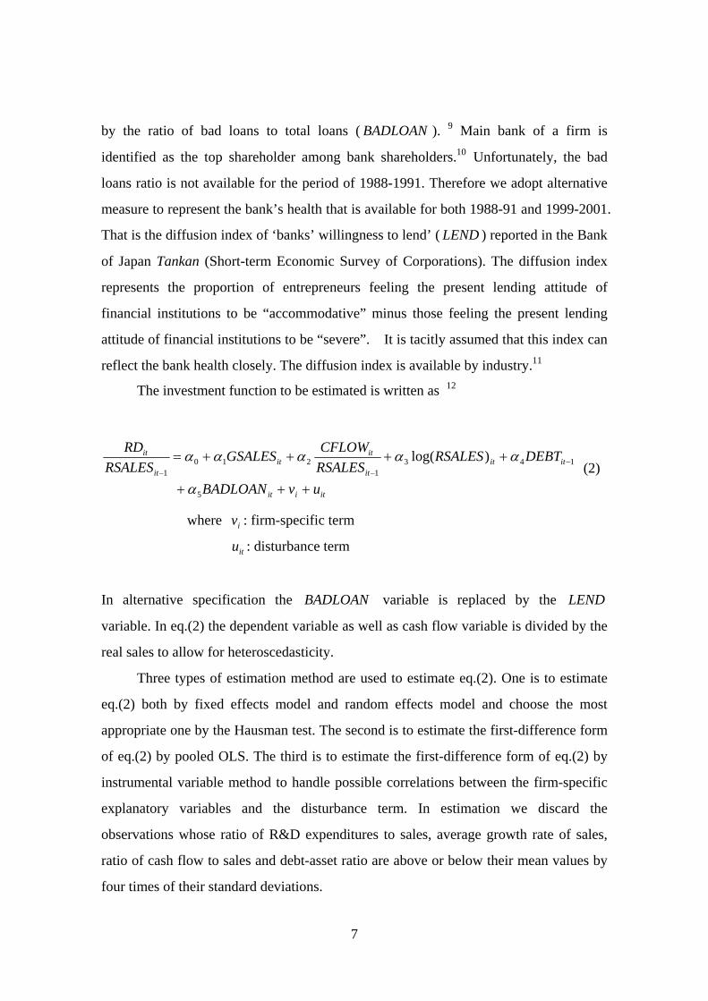
The investment function to be estimated is written as 12

itiit

ititit

itit

it

it

uvBADLOAN

DEBTRSALESRSALESCFLOWGSALES

RSALESRD

+++

++++= −−−

5

1431

2101

)log(

α

ααααα (2)

where iv : firm-specific term

itu : disturbance term

In alternative specification the BADLOAN variable is replaced by the LEND

variable. In eq.(2) the dependent variable as well as cash flow variable is divided by the

real sales to allow for heteroscedasticity.

Three types of estimation method are used to estimate eq.(2). One is to estimate

eq.(2) both by fixed effects model and random effects model and choose the most

appropriate one by the Hausman test. The second is to estimate the first-difference form

of eq.(2) by pooled OLS. The third is to estimate the first-difference form of eq.(2) by

instrumental variable method to handle possible correlations between the firm-specific

explanatory variables and the disturbance term. In estimation we discard the

observations whose ratio of R&D expenditures to sales, average growth rate of sales,

ratio of cash flow to sales and debt-asset ratio are above or below their mean values by

four times of their standard deviations.

8

Table 4 and 5 report the estimation results of eq.(2) for 1999-2001 and 1988-91,

respectively. The estimation results of fixed effects model are quite similar to those by

pooled OLS in first-differenced form. The estimation results by the instrumental

variable method in first differenced form are somewhat less precise in the sense that

most of the coefficient estimates have larger standard errors. This might be due to

reduced sample size and low correlation of instruments with the explanatory variables.

In fact, the sample size is about one-third of the fixed effects model.

It turns out that three variables are significant determinants of investment on

R&D for 1999-2001. First, the average growth rate of sales has positive effect on

investment on R&D. Second, cash flow exerts positive effect on investment on R&D.

Third, debt-asset ratio has negative effect on R&D investment, implying that massive

debt outstandings deter R&D activities. Contrasted with the significantly negative effect

of debt on R&D investment, bank health has no discernible effect on R&D investment.

It implies that even if the bank’s balance sheet deteriorates, it will not necessarily

aggravate real activities of the firm by reducing lending. The coefficient of logarithm of

real sales is negative for some cases, but insignificant.

Contrary to significantly negative effects of debt-asset ratio on R&D investment

for 1999-2001, the effect of debt-asset ratio on R&D investment is insignificant for

1988-91, irrespective of estimation method, as is seen in Table 5. To sum up, it is only

in the 90s that debt was a heavy burden for the firm in implementing R&D investment.

4. Does R&D Investment Matter in Raising the Firm-level TFP Growth?

Given our findings that debt had negative effects on R&D activities of the

Japanese research-intensive firms in the 90s, the question to be posed is “Does R&D

matter in raising the firm-level TFP growth?” If the answer is yes, then we can conclude

that massive debt outstandings of the firm in the 90s led to a decrease in the firm-level

TFP growth by deterring R&D investment. We examine this link between R&D

investment and the firm-level TFP growth in this section.

First we derive the regression equation to relate the firm-level TFP growth rate

given by eq.(1) to R&D investment with market structure and technology specific to

9

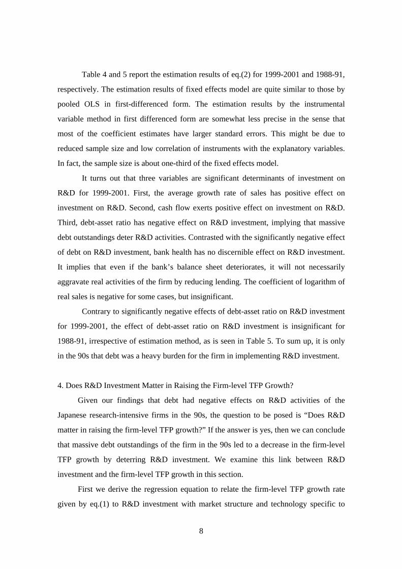
each industry into consideration. 13 14 Let us denote the value-added production

function by

),,( tLKFY ititiit = (3)

where itY : real value-added of the i-th firm in year t

itK : capital stock of the i-th firm in year t

itL :labor input of the i-th firm in year t

t :time trend

Differentiating eq.(3) with respect to time and expressing in terms of the rate of change,

we obtain the following equation.

tF

Yl

LF

YLk

KF

YKy i

itit

it

i

itit

it

i

itit ∂

∂∂∂ 1

+∆∂∂

+∆

=∆ (4)

where ititit lky ∆∆∆ ,, : rate of change in value-added, capital stock

and labor of the i-th firm in year t, respectively

The last term of the right-hand-side of eq.(4) is Solow’s residual or the TFP growth rate,

denoted by *itε∆ . Given output, the demand for inputs is determined by static cost

minimization as follows: 15

itkit

iit r

KF

,=∂∂λ

(5)

itit

iit w

LF

=∂∂λ

where itkr , : rental price of capital of the i-th firm in year t

itw : wage rate of the i-th firm in year t

itλ : marginal cost of the i-th firm in year t

10

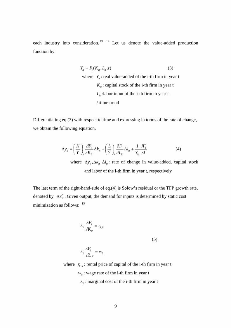
Substituting eqs.(5) into eq.(4) and arranging terms, we have

*itit

itit

it

kit l

YwLk

YKry ε

λλ∆+∆

+∆

=∆ (6)

Moreover, when the production function is homogeneous of degree m, the following

equation is obtained.

itit

k

YwL

YKrm

+

=

λλ (7)

Substitution of eq.(7) into eq.(6) yields the following expression.

( ) *, ititititLitit klkmy εµα ∆+∆−∆+∆=∆ (8)

where it

itL pYwL

=,α : labor share of value-added of the i-th firm

in year t

it

p

=λ

µ ：ratio of output price to marginal cost or

mark-up ratio.

We assume that the value ofµ , mark-up ratio, is constant over time for each industry. It

exceeds unity under imperfect competition of product market. We specify the TFP

growth rate as a function of the ratio of investment on R&D to sales. Linearizing this

relationship, we have the final expression to be estimated as follows:

( ) ititi

ititititLitit uv

RSALESRDklky ++

+∆−∆+∆+=∆

−1,3,210 βαβββ (9)

where m=1β

µβ =2

11

iv :firm-specific term

itu : disturbance term

Based on the panel data set used in the previous sections, we estimate eq.(9) that

takes account of the differences of market structure and production technology

underlying individual industry. Specifically, we replace the second term and the third

term of the right-hand-side of eq.(9) by the dummy variable for each industry multiplied

by itk∆ and ( )itititL kl ∆−∆,α , respectively. The coefficient estimate of

−1,ti

itRSALES

RD can measure the extent to which investment on R&D affects the

firm-level TFP growth rate.

Equation (9) is estimated for the two periods: 1988-91 and 1999-2001 by three

estimation procedures. One is to estimate it both by fixed effects model and random

effects model and choose the most appropriate one by the Hausman test. The second is

to estimate the first-difference form by pooled OLS. The third is to estimate the

first-difference form by instrumental variable method. 16 Table 6 and 7 show the

estimation results of eq.(9) for 1999-2001 and 1988-91, respectively. The effect of

development and research investment on the firm-level TFP growth rate is significantly

positive for 1999-2001 as well as for 1988-91. However, the impact of R&D investment

on the TFP growth rate for 1999-2001 is 6.7 to 15.2 times as large as that for 1988-91.

A ten-percentage-point increase of debt-asset ratio lowers the firm-level TFP growth

rate by 0.84 percentage point for 1999-2001 by way of withering R&D activities, while

the firm-level TFP growth rate remains almost intact for 1988-91.17

Combining the findings in the previous section that debt-asset ratio affects R&D

investment in significantly negative manner in the period of 1999-2001, but not in the

period of 1988-91 with more important role of R&D activities in the firm-level TFP

growth rate in the period of 1999-2001, we may conclude that the firm-level TFP

growth rate is much more affected by debt for 1999-2001.

Furthermore, we can explain why the distribution of the firm-level TFP growth

rate became more dispersed in the late 90s, as was seen in Section 2. First, let us note

12

that the distribution of debt-asset ratio is also more dispersed for 1999-2001. In fact the

standard deviation of the debt-asset ratio of our panel data set is 0.2057 and 0.1688 for

1999-2001 and 1988-91, respectively.18 Use of the estimation results of investment

functions of R&D and the firm-level TFP growth rate equations enables us to compare

the firm-level TFP growth rate between the two firms with the same attributes but

debt-asset ratio. Consider a firm with the debt-asset ratio on the 1st quartile, and another

with the debt-asset ratio on the 3rd quartile. Using the interquartile value of debt-asset

ratio, we can compute the difference between the firm-level TFP growth rates of the two

firms. The interquartile value of debt-asset ratio is 0.3079 and 0.2500 for 1999-2001

and 1988-91, respectively. Therefore the TFP growth rate of the 3rd quartile firm is

lower than that of the 1st quartile firm by 2.6 percentage points for 1999-2001 and is

higher only by 0.02 percentage points for 1988-91.19 To sum up, massive debt

outstandings in the 90s give rise to more dispersed distribution of the firm-level TFP

growth rate across firms.

5. Concluding Remarks

Based on the panel data of Japanese research-intensive manufacturing firms, we

investigated the R&D activities in the 90s. Main findings are follows. First, massive

debt accumulation had a negative effect on R&D investment in the late 90s, although

debt outstandings had little effect on R&D investment in the late 80s. Second,

investment on R&D was closely linked to the firm-level TFP growth rate in the late 90s,

while the link was much weaker in the late 80s.

Our findings suggest that lingering debt outstandings are in part responsible for

slowdown of the firm-level TFP growth rate in the 90s. Moreover, we have important

implications for the distributional aspect of the firm-level TFP growth rate. The

distribution of the firm-level TFP growth rate across firms is more dispersed in the 90s,

which is due to more dispersed distribution of the debt-asset ratio across firms in the 90s.

It is true that the average debt-asset ratio of Japanese large manufacturing firms is

declining over the 90s, but there still remain a number of firms that have massive debt

outstandings to be cleaned up. Policy actions to prompt the clean-up of the debt

13

outstandings in the corporate sector will be an urgent agenda for policy makers to

recover higher growth potentials of the Japanese economy.

14

Footnotes

1 See Data Appendix for the procedures to construct the variables used in the text. 2 All the parameters estimates of the Cobb-Douglas production function as well as the related statistics are shown in Table Appendix. 3 See Cohen and Levin (1989) and Cohen (1995) for comprehensive survey of the determinants of R&D activities in empirical context. 4 Internal funds turn out to be a significant explanatory variable for investment function of R&D in the studies of Hall(1992), Himmerberg and Petersen(1994) and Ozkan(2002) for the U.S. and Goto et al.(2002) for Japan. 5 Empirical support for negative effect of firm leverage on fixed investment is seen in Lang et al. (1996). Cantor(1990) and Calomiris et al.(1997) show in a slightly different context that investment of leverage firm is more responsive to sales and cash flow. For negative effects of leverage on investment on R&D, see Bronwyn Hall(1990, 1992). 6 See Myers(1977) and Hart(1995) for more detailed discussion on debt overhang. 7 Hoshi et al. (1991) is a pioneering work to show that the firms affiliated with main bank enjoy lower external finance premium than independent firms using the micro data of firms. 8 Gibson(1995 and 1997) and Kang and Stulz(2000) examine the effect of bank health on investment behavior of the Japanese firms based on micro data of firms. 9 The bad loan is defined as the sum of bankrupt loans, delayed loans, and loans delayed more than three months and mitigated loans. The data is taken from Analysis of Financial Statements of All Banks (Japanese Bankers Association). 10 We assume that main bank of a firm holds more than 2 % of total shares of the firm, so that banks with less than 2 % share of the firm is not identified as the firm’s main bank even if the bank is top shareholder among bank shareholders. 11 For empirical studies to use the Bank of Japan diffusion index of ‘banks’ willingness to lend,’ see Motonishi and Yoshikawa (1999) and Ogawa (2003a,b). Using the aggregate data, Motonishi and Yoshikawa obtain the evidence that bank lending is a significant determinant of business investment of small firms, but not large firms. On the other hand, Ogawa(2003a,b), using the firm’s micro data, found that lending attitude of financial institutions affected fixed investment and employment adversely.

15

12 The subscript i and t refers to the i-th firm and fiscal year t, respectively. 13 The following discussion originates from Solow(1957) and Robert Hall(1988,1990). For empirical analysis to follow Hall’s approach to estimate the mark-up ratios in Japan, see Ariga et al.(1992) and Baba(1995). 14 Alternative way to estimate the impact of R&D investment on productivity is to specify functional form of production function. The empirical analysis along this line based on Japanese firm data is Odagiri and Iwata(1986), Goto and Suzuki(1989), Griliches and Mairesse(1990) and Kwon and Inui(2003). 15 Basu and Kimball(1997) extend the analysis along this line to the dynamic cost minimization case with adjustment cost of quasi-fixed factors taken into consideration. 16 The estimation results by instrumental variable method in the first-differenced form are not reported here since we were unable to obtain precise coefficient estimates. 17 The figures are computed on the basis of parameters obtained from fixed effects model with banks’ willingness to lend as banks’ health variable for R&D investment function and fixed effects model for TFP growth rate regression for 1999-2001 and 1988-91. 18 When we measure the dispersion of the distribution of debt-asset ratio by coefficient of variation, it is 0.3895 and 0.2721 for 1999-2001 and 1988-91, respectively. 19 For the models used for computing the differences of the TFP growth rate, see footnote 17.

16

Data Appendix

We give brief explanations of the data construction procedures with special

emphasis on capital stock.

Construction of Capital Stock

Our basic strategy to construct a series of the physical depreciable capital stock

is to follow the perpetual inventory method, as discussed in Hayashi and Inoue(1991) .

The capital stock series is constructed each for six types of assets: nonresidential

buildings, structures, machinery, vessels, transportation equipment except vessels,

instruments and tools to add up the total capital stock. Our benchmark year is the fiscal

year of 1985 and 1995 for 1988-91 and 1999-2001, respectively. Benchmark stock is

converted into the real value by dividing the book-valued stock by the investment goods

deflator in benchmark year minus the average years elapsed since installation. The

information of the average years elapsed since installation is available from 1970

National Wealth Survey for each type of physical depreciable assets. The investment

goods deflator is constructed for each industry and each type of physical asset by

making use of the Fixed Capital Formation Matrix in the 1995 Input-Output tables.

Nominal investment is constructed for each type of physical asset as follows:

( )( ) ( ){ }

( ) ( ) ititititit

ititititititit

itititit

DEPADADKGKGADDEPADKGINCKGINC

DDSRINCNI

+−−−=−+−−+−=

−−=

−−

−−

11

11 (A-1)

where itNI : nominal investment of the i-th firm in year t

itINC : increment of physical asset of the i-th firm in year t

itSR : value of the i-th firm’s physical asset scrapped in year t

itDD : value of the i-th firm’s physical asset scrapped in year t

out of the accumulated depreciation

itKG : i-th firm’s physical asset at the end of year t at purchase

value

17

itAD : accumulated depreciation of the i-th firm in year t

itDEP : depreciation of the i-th firm in year t

Nominal investment is divided by the corresponding investment goods deflator to obtain

real investment ( itI ). The physical depreciation rates (δ ) are based on those reported in

Hayashi and Inoue(1991). They show the rates for five categories of assets, which were

derived from Hulten and Wykoff(1979,1981). They are 4.7 % per annum for

nonresidential buildings, 5.64 % for structures, 9.489 % for machinery, 14.7 % for

transportation equipment, and 8.8838 % for instruments and tools. We use the

depreciation rate of transportation equipment for that of vessels.

Given the benchmark value of depreciable stock, real investment series, and

depreciation rate, we obtain the capital stock of each type from the following formula.

For detailed explanations see Hayashi and Inoue(1991).

ititit IKK +−= −1)1( δ (A-2)

where itK : i-th firm’s capital stock at the end of year t

Finally, the capital stock is multiplied by the capacity utilization rate index

reported by Ministry of Economy, Trade and Industry.

Value-added

Value-added = (Ordinary Income – Corporate Taxes – Enterprise Tax – Residential

Tax + Compensations to Directors + Wages and Salaries to Employees + Welfare

Expenses + Reserve Fund for Bonuses + Retirement Allowance + Reserve Fund for

Retirement Allowance + Company Pension + Taxes + Rental Fees + Royalties +

Interest and Discount paid + Depreciation Allowances).

Labor inputs

The number of employees is multiplied by the Hours Worked Indices (Total

Hours Worked) reported in Monthly Labour Survey (Ministry of Health, Labour and

18

Welfare).

Labor Share

Labor share = (Compensations to Directors + Wages and Salaries to Employees

+ Welfare Expenses + Reserve Fund for Bonuses + Retirement Allowance + Reserve

Fund for Retirement Allowance + Company Pension)/Value-added.

Investment on R&D

Total expenditure on R&D.

Real sales

Nominal sales are divided by the Corporate Goods Price Indexes of each

industry (The Bank of Japan).

Cash flow

Cash flow = (ordinary income + depreciation allowance – corporate tax –

dividends paid – compensations and bonus to directors).

Debt-asset ratio

Liabilities are divided by total assets.

Bad loans ratio

Bad loans ratio of the firm’s main bank is defined as the ratio of bad loans to total

loans. Main bank of the firm is identified as the top shareholder among bank

shareholders. The bad loan is defined as the sum of bankrupt loans, delayed loans, and

loans delayed more than three months and mitigated loans. The data of bad loans comes

from Analysis of Financial Statements of All Banks (Japanese Bankers Association).

The diffusion index of ‘banks’ willingness to lend’

The diffusion index is the proportion of entrepreneurs feeling the present lending

19

attitude of financial institutions to be “accommodative” minus those feeling the present

lending attitude of financial institutions to be “severe”. It is reported by the Bank of

Japan Tankan (Short-term Economic Survey of Corporations).

20

References

[1] Ariga,K., Kaneko,T., Sakamoto,K. and H.Sano(1992).” Business Cycles of the

Post-war Japan: Price, Wage and Mark-up,” Financial Review 22 (Policy Research

Institure, Ministry of Finance), pp.130-161. (in Japanese)

[2] Baba,N.(1995),” Causes of Price Differentials between Domestic and Foreign

Goods: Empirical Investigation through Mark-up Pricing,” Monetary and Economic

Studies (The Bank of Japan) Vol.14, No.2, pp.71-97. (in Japanese)

[3] Basu,S. and M.S.Kimball(1997).” Cyclical Productivity with Unobserved Input

Variations,” NBER Working Paper No.5915.

[4] Calomiris, C.W., Orphanides, A., and S.A. Sharpe(1997).” Leverage as a State

Variable for Employment, Inventory Accumulation, and Fixed Investment,” In Capie,F.,

and G.E.Wood (eds.) Asset Prices and the Real Economy (St. Martin’s Press: New York),

pp.169-193.

[5] Cantor, R.(1990).” Effects of Leverage on Corporate Investment and Hiring

Decisions,” Federal Reserve Bank of New York Quarterly Review 15, pp.31-41.

[6] Cohen,W.M.(1995).” Empirical Studies of Innovative Activity,” In Stoneman, P.,

(ed.) Handbook of The Economics of Innovation and Technological Change (Blackwell:

Oxford) pp.182-264.

[7] Cohen,W.M. and R.C. Levin (1989).” Empirical Studies of Innovation and Market

Structure,” In Schmalensee, R.C. and R.D. Willig (eds.) Handbook of Industrial

Organization Vol.2 (North Holland: Amsterdam)

[8] Fukao, K. and H.U. Kwon(2003).” The Productivity and the Economic Growth of

21

Japan: Empirical Analysis Based on Industry-Level and Firm-level Data,” paper

presented at Semi-annual Conference of Japanese Economic Association held at Oita.

[9] Gibson,M.S.(1995).” Can Bank Health Affect Investment? Evidence from Japan,”

Journal of Business 68, pp.281-308.

[10] Gibson,M.S.(1997).” More Evidence on the Link between Bank Health and

Investment in Japan,” Journal of the Japanese and International Economies 11,

pp.296-310.

[11] Goto, A. and K. Suzuki(1989),” R&D Capital, Rate of Return on R&D Investment

and Spillover of R&D in Japanese Manufacturing,” Review of Economics and Statistics

71, pp.555-564.

[12] Goto, A., Koga, T. and K. Suzuki(2002),” Determinants of Industrial R&D in

Japanese Manufacturing Industries,” The Economic Review (Institute of Economic

Research, Hitotsubashi University), Vol.53, No.1, pp.18-23. (in Japanese)

[13] Griliches,Z. and J. Mairesse(1990).” R&D and Productivity Growth: Comparing

Japanese and US Manufacturing Firms, in Griliches,Z.(ed.) R&D, Patens, and

Productivity (University of Chicago Press: Chicago, IL,USA) pp.317-348.

[14] Hall,B.H.(1990).” The Impact of Corporate Restructuring on Industrial Research

and Development,” Brookings Papers on Economic Activity, Special Issue,pp.85-124.

[15] Hall,B.H.(1992).” Investment and R&D at the Firm Level: Does the Source of

Financing Matter?” NBER Working Paper No.4096.

[16] Hall,R.E.(1988).” The Relation between Price and Marginal Cost in U.S. Industry,”

Journal of Political Economy 96, pp.921-947.

22

[17] Hall,R.E.(1990).” Invariance Properties of Solow’s Productivity Residual,” in

Diamond,P.(ed.) Growth/Productivity/Unemployment: Essays to Celebrate Bob Solow’s

Birthday (MIT Press: Cambridge, MA, USA) .

[18] Hart, O.(1995). Firms, Contracts and Financial Structure, Oxford Clarendon

Press.

[19] Hayashi, F. and T. Inoue(1991)." The Relation between Firm Growth and Q with

Multiple Capital Goods: Theory and Evidence from Panel Data on Japanese Firms,"

Econometrica 59, pp.731-753.

[20] Hayashi,F. and E.C.Prescott(2002).” The 1990s in Japan: A Lost Decade,” Review

of Economic Dynamics Vol.5, No.1, pp.206-235.

[21] Himmerberg C.P. and B.C.Petersen(1994).” R&D and Internal Finance: A Panel

Study of Small Firms in High-Tech Industries,” Review of Economics and Statistics 76,

pp.38-51.

[22] Hoshi, T., Kashyap, A., and D.Scharfstein(1991)." Corporate Structure, Liquidity,

and Investment: Evidence from Japanese Industrial Groups," Quarterly Journal of

Economics 106, pp.33-60.

[23] Hulten,C., and F.Wykoff(1979). “ Economic Depreciation of the U.S. Capital

Stock,” Report Submitted to U.S. Department of Treasury, Office of Tax Analysis,

Washington,D.C.

[24] Hulten,C., and F.Wykoff(1981). " The Measurement of Economics Depreciation ,"

C.Hulten (ed.) Depreciation, Inflation and the Taxation of Income from Capital, Urban

Institute.

23

[25] Kang, J.K. and R.S. Stulz(2000).” Do Banking Shocks Affect Borrowing Firm

Performance? An Analysis of the Japanese Experience,” Journal of Business 73,

pp.1-23. .

[26] Kwon,H.U. and T.Inui(2003).” R&D and Productivity Growth in Japanese

Manufacturing Firms,” ESRI Discussion Paper Series No.44.

[27] Lang, L., Ofek,E. and R.M.Stulz(1996).” Leverage, Investment, and Firm Growth,”

Journal of Financial Economics 40, pp.3-29.

[28] Motonishi, T. and H. Yoshikawa(1999).” Causes of the Long Stagnation of Japan

during the 1990’s: Financial or Real?” Journal of the Japanese and International

Economies 13, pp.181-200.

[29] Myers, S.C.(1977).” Determinants of Corporate Borrowing,” Journal of Financial

Economics 5, pp.147-175.

[30] Nishimura,G.K., Nakajima,T. and K. Kiyota(2003).” What Happened to the

Japanese Industry during a Lost Decade? : Entry and Exit of Firms and TFP,” RIETI

Discussion Paper Series 03-J-002. (in Japanese)

[31] Odagiri,H. and H.Iwata(1986).” The Impact of R&D on Productivity Increase in

Japanese Manufacturing Companies,” Research Policy 15, pp.13-19.

[32] Ogawa,K. (2003a),” Financial Distress and Employment: The Japanese Case in the

90s,” NBER Working paper No. 9646.

[33] Ogawa,K. (2003b),” Financial Distress and Corporate Investment: The Japanese

Case in the 90s,” Osaka University ISER Discussion Paper No. 584.

24

[34] Ozkan,N.(2002).” Effects of Financial Constraints on Research and Development

Investment: An Empirical Investigation,” Applied Financial Economics 12, pp.827-834.

[35] Solow,R.M.(1957).”Technological Change and the Aggregate Production

Function,” Review of Economics and Statistics 39, pp.312-320.

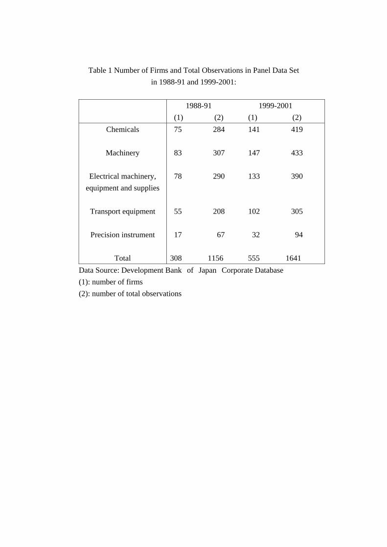
Table 1 Number of Firms and Total Observations in Panel Data Set in 1988-91 and 1999-2001:

1988-91 1999-2001

(1) (2) (1) (2) Chemicals

Machinery

Electrical machinery,

equipment and supplies

Transport equipment

Precision instrument

Total

75 284 141 419 83 307 147 433 78 290 133 390 55 208 102 305 17 67 32 94 308 1156 555 1641

Data Source: Development Bank of Japan Corporate Database (1): number of firms (2): number of total observations

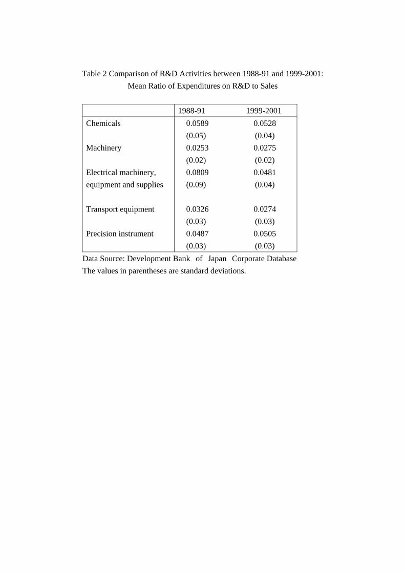
Table 2 Comparison of R&D Activities between 1988-91 and 1999-2001: Mean Ratio of Expenditures on R&D to Sales

1988-91 1999-2001 Chemicals Machinery Electrical machinery, equipment and supplies Transport equipment Precision instrument

0.0589 0.0528 (0.05) (0.04) 0.0253 0.0275 (0.02) (0.02) 0.0809 0.0481 (0.09) (0.04)

0.0326 0.0274 (0.03) (0.03) 0.0487 0.0505 (0.03) (0.03)

Data Source: Development Bank of Japan Corporate Database The values in parentheses are standard deviations.

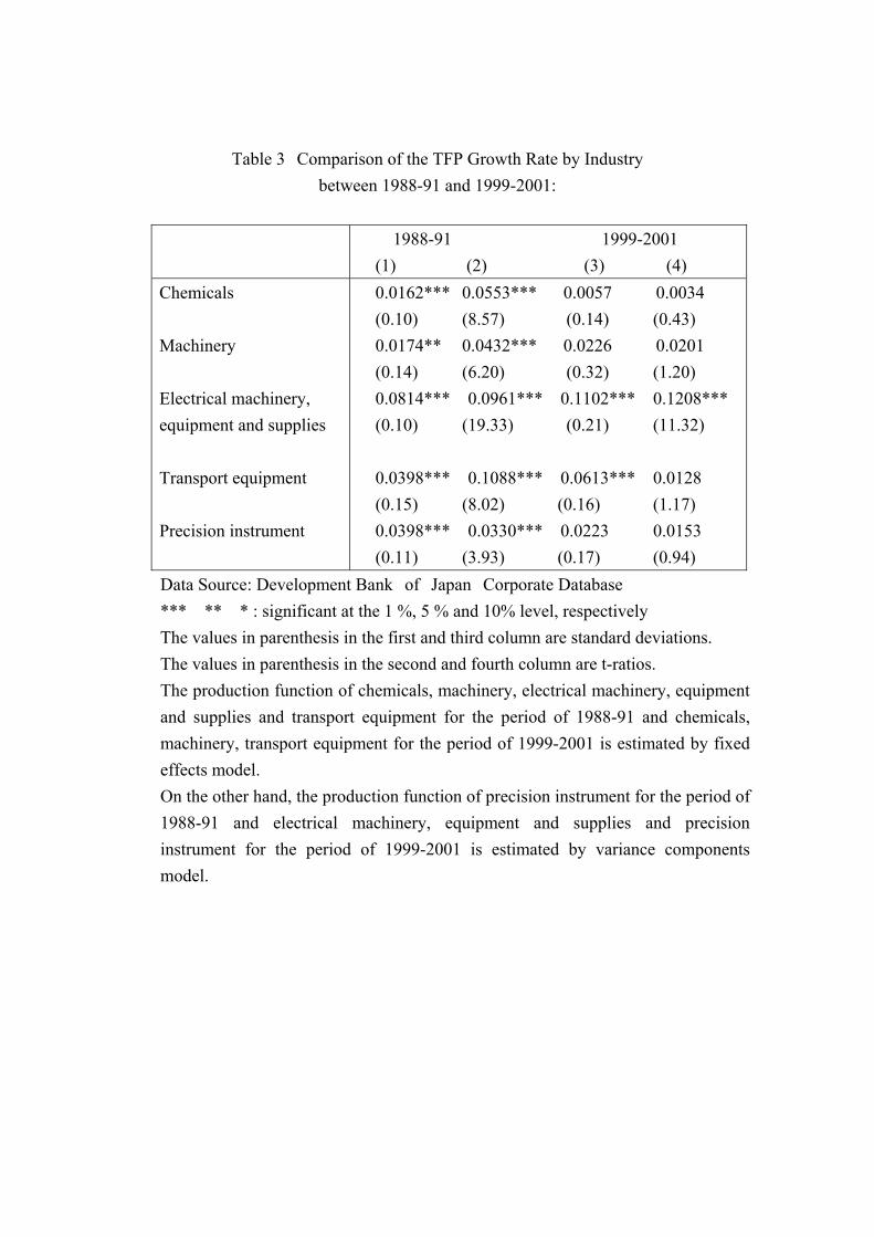
Table 3 Comparison of the TFP Growth Rate by Industry between 1988-91 and 1999-2001:

1988-91 1999-2001

(1) (2) (3) (4) Chemicals Machinery Electrical machinery, equipment and supplies Transport equipment Precision instrument

0.0162*** 0.0553*** 0.0057 0.0034 (0.10) (8.57) (0.14) (0.43) 0.0174** 0.0432*** 0.0226 0.0201 (0.14) (6.20) (0.32) (1.20) 0.0814*** 0.0961*** 0.1102*** 0.1208*** (0.10) (19.33) (0.21) (11.32)

0.0398*** 0.1088*** 0.0613*** 0.0128 (0.15) (8.02) (0.16) (1.17) 0.0398*** 0.0330*** 0.0223 0.0153 (0.11) (3.93) (0.17) (0.94)

Data Source: Development Bank of Japan Corporate Database *** ** * : significant at the 1 %, 5 % and 10% level, respectively The values in parenthesis in the first and third column are standard deviations. The values in parenthesis in the second and fourth column are t-ratios. The production function of chemicals, machinery, electrical machinery, equipment

and supplies and transport equipment for the period of 1988-91 and chemicals, machinery, transport equipment for the period of 1999-2001 is estimated by fixed effects model.

On the other hand, the production function of precision instrument for the period of 1988-91 and electrical machinery, equipment and supplies and precision instrument for the period of 1999-2001 is estimated by variance components model.

Table 4 Estimation Results of R&D Investment Function: 1999-2001

Estimation method

Growth rate Cash Real Debt-asset Ratio of Banks’ willingness S.E. of sales flow sales ratio bad loans to lend Number of observations

1. Fixed effects model 2.Fixed effects model 3.First difference (Pooled OLS) 4.First difference (Pooled OLS) 5. First difference (Instrumental variables) 6. First difference (Instrumental variables)

0.0228** 0.0509*** -0.0048 -0.0190*** 0.0041 0.0074 (2.35) (5.92) (-1.44) (-3.52) (1.08) 1603

0.0190** 0.0514*** -0.0042 -0.0230*** -0.0040 0.0075 (1.97) (5.63) (-1.24) (-3.89) (-0.57) 1480

0.0297*** 0.0359*** -0.0018 -0.0153*** 0.0042 0.0093 (3.01) (4.54) (-0.53) (-2.80) (1.19) 1057

0.0264*** 0.0360*** -0.0006 -0.0175*** -0.0027 0.0095 (2.67) (4.16) (-0.39) (-2.92) (-0.39) 964

0.0017 -0.0475 0.0252* -0.0265 0.0252*** 0.0091 (0.10) (-0.91) (1.73) (-1.00) (3.90) 534

0.0350* -0.0410 0.0192 -0.0642* -0.0044 0.0098 (1.76) (-0.63) (1.08) (-1.91) (-0.40) 485

Notes: *** ** * : significant at the 1 %, 5 % and 10% level, respectively The values in parenthesis are t-ratios.

Instruments for the 5-th and 6-th row are constant, second-lagged and third-lagged cash flow ratios, average growth rates of sales, debt-asset ratios and logarithm of real sales. It is assumed that banks’ willingness to lend is exogenous in the 5-th equation and that the bank’s bad loan ratio is exogenous in the 6-th equations. .

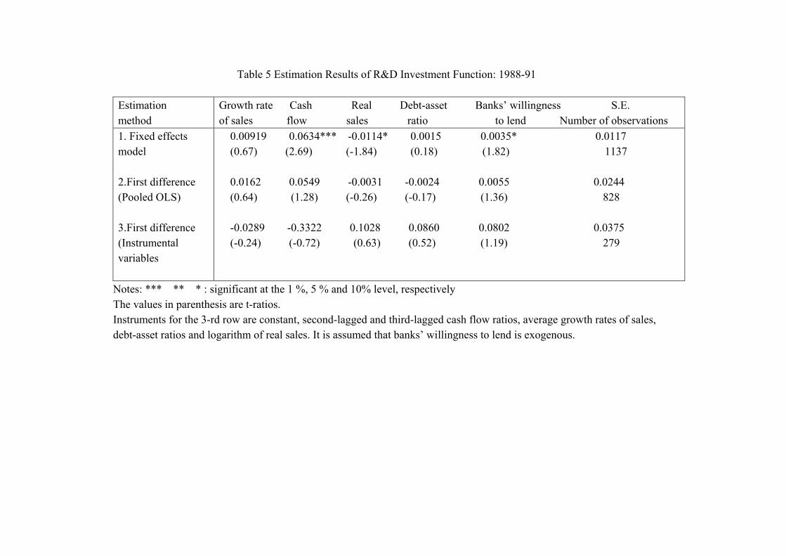
Table 5 Estimation Results of R&D Investment Function: 1988-91

Estimation method

Growth rate Cash Real Debt-asset Banks’ willingness S.E. of sales flow sales ratio to lend Number of observations

1. Fixed effects model 2.First difference (Pooled OLS) 3.First difference (Instrumental variables

0.00919 0.0634*** -0.0114* 0.0015 0.0035* 0.0117 (0.67) (2.69) (-1.84) (0.18) (1.82) 1137

0.0162 0.0549 -0.0031 -0.0024 0.0055 0.0244 (0.64) (1.28) (-0.26) (-0.17) (1.36) 828

-0.0289 -0.3322 0.1028 0.0860 0.0802 0.0375 (-0.24) (-0.72) (0.63) (0.52) (1.19) 279

Notes: *** ** * : significant at the 1 %, 5 % and 10% level, respectively The values in parenthesis are t-ratios.

Instruments for the 3-rd row are constant, second-lagged and third-lagged cash flow ratios, average growth rates of sales, debt-asset ratios and logarithm of real sales. It is assumed that banks’ willingness to lend is exogenous.

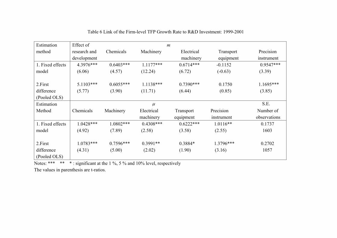
Table 6 Link of the Firm-level TFP Growth Rate to R&D Investment: 1999-2001

Estimation method

Effect of m research and Chemicals Machinery Electrical Transport Precision development machinery equipment instrument

1. Fixed effects model 2.First difference (Pooled OLS)

4.3976*** 0.6403*** 1.1177*** 0.6714*** -0.1152 0.9547*** (6.06) (4.57) (12.24) (6.72) (-0.63) (3.39) 5.1103*** 0.6055*** 1.1138*** 0.7390*** 0.1750 1.1695*** (5.77) (3.90) (11.71) (6.44) (0.85) (3.85)

Estimation Method

µ S.E. Chemicals Machinery Electrical Transport Precision Number of machinery equipment instrument observations

1. Fixed effects model 2.First difference (Pooled OLS)

1.0428*** 1.0802*** 0.4308*** 0.6222*** 1.0116** 0.1737 (4.92) (7.89) (2.58) (3.58) (2.55) 1603

1.0783*** 0.7596*** 0.3991** 0.3884* 1.3796*** 0.2702 (4.31) (5.00) (2.02) (1.90) (3.16) 1057

Notes: *** ** * : significant at the 1 %, 5 % and 10% level, respectively The values in parenthesis are t-ratios.

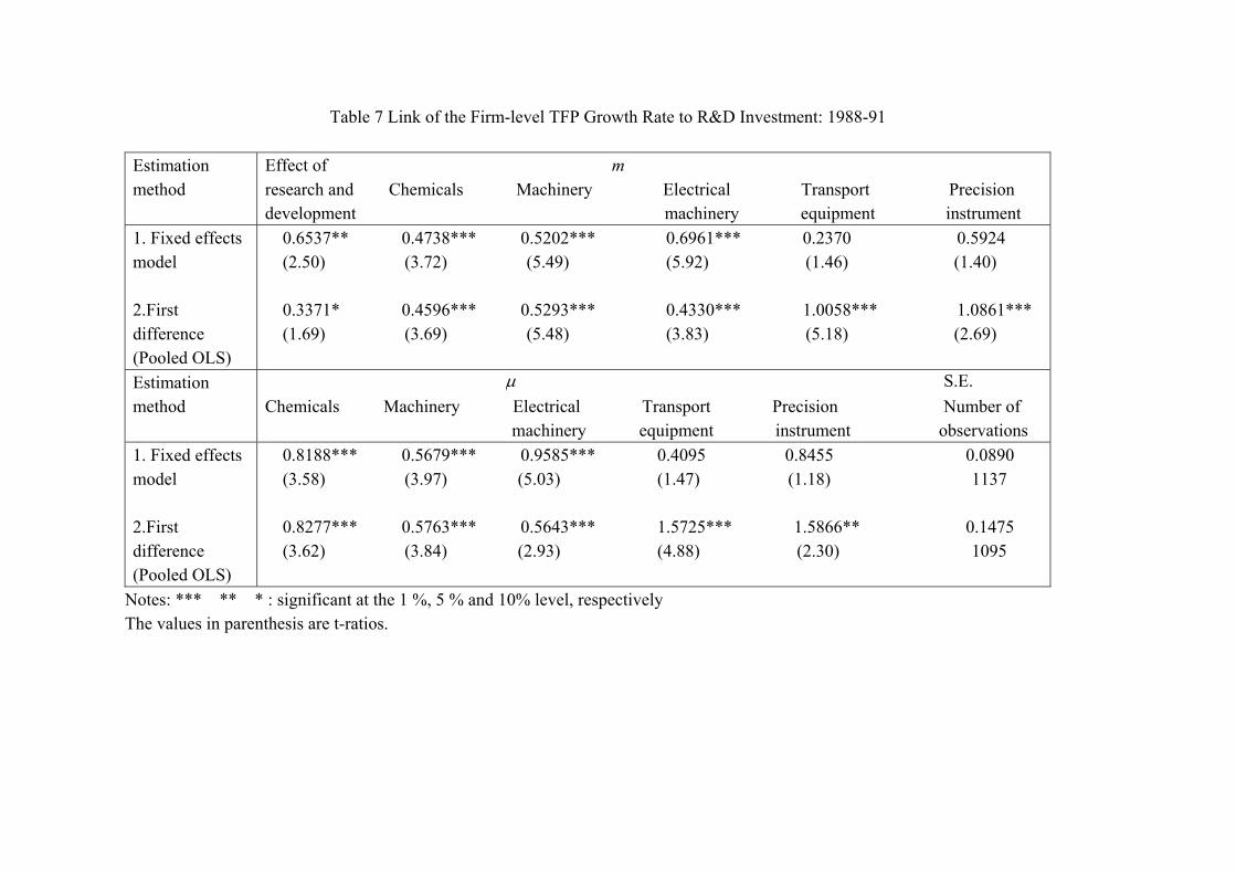
Table 7 Link of the Firm-level TFP Growth Rate to R&D Investment: 1988-91

Estimation method

Effect of m research and Chemicals Machinery Electrical Transport Precision development machinery equipment instrument

1. Fixed effects model 2.First difference (Pooled OLS)

0.6537** 0.4738*** 0.5202*** 0.6961*** 0.2370 0.5924 (2.50) (3.72) (5.49) (5.92) (1.46) (1.40) 0.3371* 0.4596*** 0.5293*** 0.4330*** 1.0058*** 1.0861*** (1.69) (3.69) (5.48) (3.83) (5.18) (2.69)

Estimation method

µ S.E. Chemicals Machinery Electrical Transport Precision Number of machinery equipment instrument observations

1. Fixed effects model 2.First difference (Pooled OLS)

0.8188*** 0.5679*** 0.9585*** 0.4095 0.8455 0.0890 (3.58) (3.97) (5.03) (1.47) (1.18) 1137

0.8277*** 0.5763*** 0.5643*** 1.5725*** 1.5866** 0.1475 (3.62) (3.84) (2.93) (4.88) (2.30) 1095

Notes: *** ** * : significant at the 1 %, 5 % and 10% level, respectively The values in parenthesis are t-ratios.

Table Appendix Estimation Results of the Cobb-Douglas Production Function by Industry

1988-91 1999-2001

Labor Capital Time S.E. Labor Capital Time S.E. elasticity elasticity trend elasticity elasticity trend

Chemicals Machinery Electrical machinery, equipment and supplies Transport equipment Precision instrument

0.5894*** 0.1940*** 0.0553*** 0.0743 0.4301*** 0.2326*** 0.0034 0.1181 (6.34) (4.38) (8.57) (4.13) (3.81) (0.43) 0.3520*** 0.1519*** 0.0432*** 0.0931 0.2702 0.3654** 0.0201 0.2533 (2.93) (4.07) (6.20) (1.61) (2.52) (1.20) 0.9530*** 0.1535*** 0.0961*** 0.0663 0.6770*** 0.3511*** 0.1208*** 0.2682 (12.25) (5.96) (19.33) (17.30) (11.25) (11.32) 1.1336*** -0.1327 0.1088*** 0.0973 0.4609*** 0.3003*** 0.0128 0.0968 (7.73) (-1.50) (8.02) (7.12) (2.94) (1.17) 0.7193*** 0.2311*** 0.0330*** 0.1568 0.7119*** 0.3138*** 0.0153 0.2619 (9.18) (4.21) (3.93) (6.92) (4.25) (0.94)

*** ** * : significant at the 1 %, 5 % and 10% level, respectively The values in parenthesis are t-ratios. The production function of chemicals, machinery, electrical machinery, equipment and supplies and transport equipment for the

period of 1988-91 and chemicals, machinery, transport equipment for the period of 1999-2001 is estimated by fixed effects model. On the other hand, the production function of precision instrument for the period of 1988-91 and electrical machinery, equipment

and supplies and precision instrument for the period of 1999-2001 is estimated by variance components model.

Data Source: Survey of Research and Development (Statistics Bureau of Ministry of Public Management, Home Affairs, Posts and Telecommunications)

Figure 1 Rate of Change in Intramural Expenditures on R&D:Large Firms in Manufacturing Sector

-10.00

-5.00

0.00

5.00

10.00

15.00

20.00

25.00

1981 1982 1983 1984 1985 1986 1987 1988 1989 1990 1991 1992 1993 1994 1995 1996 1997 1998 1999 2000 2001 2002

%

Data Source: Survey of Research and Development (Statistics Bureau of Ministry of Public Management, Home Affairs, Posts and Telecommunications)

Figure 2 Rate of Change in Persons Engaged in R&D Activities:Large Firms in Manufacturing Sector

-6.00

-4.00

-2.00

0.00

2.00

4.00

6.00

8.00

10.00

1981 1982 1983 1984 1985 1986 1987 1988 1989 1990 1991 1992 1993 1994 1995 1996 1997 1998 1999 2000 2001 2002

%

Data Source: Survey of Research and Development (Statistics Bureau of Ministry of Public Management, Home Affairs, Posts and Telecommunications)

Figure 3 Ratio of Intramural Exprnditures on R&D to Sales:Large Firms in Manufacturing Sector

2.00

2.50

3.00

3.50

4.00

4.50

1981 1982 1983 1984 1985 1986 1987 1988 1989 1990 1991 1992 1993 1994 1995 1996 1997 1998 1999 2000 2001 2002

%

Data Source: Survey of Research and Development (Statistics Bureau of Ministry of Public Management, Home Affairs, Posts and Telecommunications

Figure 4 Intramural Expenditure on R&D by Types:Large Firms in Manufacturing Sector

0.00

1.00

2.00

3.00

4.00

5.00

6.00

7.00

8.00

1980 1981 1982 1983 1984 1985 1986 1987 1988 1989 1990 1991 1992 1993 1994 1995 1996 1997 1998 1999 2000

Bas

ic R

esea

rch

(%)

69.00

69.50

70.00

70.50

71.00

71.50

72.00

72.50

73.00

73.50

74.00

74.50

Dev

elop

men

t Res

eatc

h (%

)

Basic Research Develoment Resaerch