Column-Generation for Design of Survivable Networks

Kavinesh Singh, University of Auckland Andy Philpott, University of Auckland

Kevin Wood, Naval Postgraduate School

July 18, 2008

Abstract

We present a model for the design of a minimum-cost, survivable electricity distribution net-

work, which generalizes to telecommunications, logistics and other network types. We formulate

this problem as a two-stage stochastic mixed-integer program in which first-stage decisions ex-

pand capacity, and recourse decisions configure and operate the network so as to be feasible

under various scenarios corresponding to individual link failures. Dantzig-Wolfe decomposition

of this formulation leads to (a) a master problem comprising binary capacity-expansion and

high-level operating decisions, and (b) mixed-integer, column-generating subproblems, which

represent deterministic network-design models. A “super-network” representation of the dis-

tribution network significantly reduces the number of binary variables, and provides tighter

linear-programming relaxations for the subproblems. Column generation with super-network

subproblems solves real-world model instances an order of magnitude faster than CPLEX can

solve the corresponding extensive models.

Keywords: Power distribution planning, power distribution reliability, integer programming

1 Introduction

This paper presents a new class of optimization models for designing minimum-cost survivable

networks, motivated by an application to electricity distribution networks. The generic model is

a two-stage, stochastic, mixed-integer program in which the first stage adds capacity increments

to existing network components while the second stage configures and operates the network under

various component-failure scenarios. By “operate” we mean that one or more commodities are

routed through the network subject to supply, demand, capacity and possibly other constraints.

For simplicity, we assume that the only components that can fail or may need additional capacity

are network links. This model can handle the option of adding completely new links by defining

existing links with no capacity, but we view the model primarily as one of capacity expansion, as

opposed to one of “from-scratch” network design.

Network-design (capacity-expansion) problems like ours are known to be NP-Hard (see

Johnson et al. [16]), but the extensive research in this field gives evidence of their significance.

Most research on survivable network design problems (SNDPs) has focused on telecommunications

1

networks; for example, see the review in Soni et al. [38]. However, SNDPs have also received some

attention in the area of electric power networks (Ramirez-Rosado et al. [28], Samarkoon et al. [31])

and logistical networks (Thadakamalla et al. [40], Snyder and Daskin [37]).

Two main factors influence the formulation of SNDP: the design strategy and the restoration

strategy. The design strategy can be classified in two ways. A sequential-design model assumes

that the capacity required for routing commodity flows in the “non-failure state” has already been

determined, and the only optimization required is that of the spare capacity required for routing

flows in “failure states.” This is also known as “spare-capacity optimization.” On the other hand,

a simultaneous-design model simultaneously optimizes capacity required for routing of flows both

in the non-failure state and in failure states. This is also known as “joint optimization.” Our

model essentially falls into the latter category, although we will describe how it could be modified

to handle certain sequential-design cases.

The restoration strategy determines how flows are rerouted in the event of a link failure:

1. link (line) restoration reroutes a disrupted commodity’s flow through an alternate sequence

of links (a path) between the end nodes of the failed link;

2. path restoration reroutes a disrupted commodity’s flow through one or more alternative

path(s) between that commodity’s origin and destination points;

3. global restoration allows rerouting of all commodity flows, disrupted or otherwise.

The SNDP literature does not deal much with global restoration because (a) most of the

literature covers telecommunications models, (b) global restoration is normally an impractical

paradigm for telecommunications because secondary disruptions can arise from the act of rerouting

undisrupted flows (Rajan and Atamturk [27]), and (c) even when appropriate, global restoration

leads to multicommodity models that become prohibitively large (Rajan and Atamturk [26]). For

these reasons, the rare telecommunications models that do incorporate global restoration are usu-

ally applied to small problems instances as benchmarks for other restoration strategies (Xiong and

Mason [45]).

Telecommunications traffic is typically modeled using a separate commodity for each origin

and destination pair. In contrast, a single commodity suffices to model electric power flowing

through a distribution network. This simplification allows our SNDP model to incorporate global

restoration without becoming too large.

Our electric-power problem poses its own computational challenges, however, because of

the following unique modeling requirement: the underlying mesh network must be configured, in

every failure scenario, by activating certain links and deactivitating others, so that the operational

network forms a tree, i.e., power must flow through a single path from the source to each destination.

Analogous telecommunications models must reroute traffic under failure scenarios, but do not

require this “reconfiguration.”

The literature on SNDPs for electricity distribution networks is modest, and mostly de-

scribes heuristics: link-exchange local search (Nara et al. [25], Kuwabara and Nara [20]), evolution-

2

ary algorithms [28], and tabu search (Ramirez-Rosado and Dominguez-Navarro [29]). An exception

is the work by Kagan and Adams [17] who solve a mathematical program with binary first-stage

capacity-expansion decisions, and (continuous) second-stage decisions that operate the network

and penalize unmet demand. However, that model does not admit binary second-stage decisions

to enforce tree-configuration requirements.

In contrast to electric power networks, the literature on SNDPs in telecommunications

networks is extensive. Heuristic approaches are common (e.g., Balakrishnan et al. [3], Ball and

Vakhutinsky [5], Gavish et al. [14], Luss and Wong [22]). Of course, the quality of heuristically

obtained solutions cannot be guaranteed, and perhaps this has motivated the recent research fo-

cusing on exact solution methods. Iraschko et al. [15] create mixed-integer programs (MIPs) for

combinations of both design strategies, with path and link restoration; Balakrishnan et al. [4]

and Kennington and Whitler [19] study sequential-design models with link restoration. The latter

two papers develop valid inequalities to strengthen the linear-programming (LP) relaxation of the

model. Kennington and Lewis [18] explore a similar solution approach with path restoration and

present a specialized branch-and-bound algorithm.

We use column generation to solve our SNDP. This technique is widely exploited to solve

SNDPs in the telecommunications industry, typically using shortest-path subproblems to generate

columns for a path-based formulation. The main class of models in this area defines a master

problem to determine link capacities and flows for the paths generated (Murakami and Kim [24],

[26], [27]). (See also Stoer and Dahl [39], Dahl and Stoer [6] and Wessaly [42].)

The use of column generation for solving stochastic integer (or mixed-integer) programs

is relatively new: Lulli and Sen [21] use branch and price (column generation plus branch and

bound) for stochastic batch-sizing problems; Shiina and Birge [34] use column generation to solve

a unit-commitment problem under demand uncertainty; Damodaran and Wilhelm [7] model high-

technology product upgrades under uncertain demand and use branch and price as a solution

technique; and Silva and Wood [35] present a branch-and-price approach for a class of two-stage

stochastic mixed-integer programs.

The master problem and subproblems we present differ substantially from those used in the

above papers. In particular, our pure integer master problem involves capacity expansion and high-

level operating decisions, while the subproblems determine the set of capacity expansions required

to ensure feasible system operation under each failure scenario.

The rest of the paper is laid out as follows. Section 2 describes some important mod-

eling issues in SNDPs for electricity distribution networks, and section 3 gives a mathematical

formulation for our specific application. Difficulty in solving this model motivates Dantzig-Wolfe

decomposition and the column-generation solution procedure described in section 4. The decompo-

sition subproblems in our SNDP are difficult mixed-integer programs, however, so section 5 shows

how to ameliorate this difficulty with a stronger “super-network formulation.” Section 6 presents

computational results and section 7 presents conclusions.

3

2 Electric Power Distribution Networks

In essence, distribution networks for electric power consist of (a) one or more power sources, i.e.,

drop-off points where the high-voltage electricity is stepped down through transformers to a lower

voltage for distribution, (b) demand points, (c) junctions, (d) switches, and (e) interconnecting

power lines. An urban distribution network may contain hundreds or even thousands of such

components. Such a network is “survivable” if it can recover from a “line fault,” i.e., the failure of

a cable or associated equipment.

Distribution networks operate in several alternative configurations including mesh, inter-

connected, link arrangement, open loop, and radial (Lakervi and Holmes [11]). We consider net-

works, with underlying mesh structure, that operate in a radial configuration. This configuration

is obtained by opening and closing switches at different points of the mesh network, so that the

connected network forms a tree with the power source as its root node. (Multiple drop-off points

are treated as a single power source.) Thus, power must flow from the power source to each demand

point following a unique path of lines, without exceeding line capacities or violating voltage-drop

standards.

In the event of a fault in an operating, radially configured network, the distribution com-

pany will typically reroute flow to restore supply to customers as rapidly as possible. (It may be

impossible to identify and repair a fault quickly, so rerouting is often the immediate response; repair

occurs later.) This rerouting is effected by opening electrical switches that isolate the faulted sec-

tion, and by then closing switches to establish alternative paths for power to flow from the source to

affected customers. This rerouting amounts to switching the operating configuration from one tree

topology to another. To enable this switching, the company builds redundancy into the network in

the form of excess line capacities. This redundancy includes lines that are not used under normal

circumstances, but are on hand to be used for “recourse,” i.e., for recovering a working, radial

configuration in the event of fault. The full set of lines forms the “underlying mesh structure.”

We say that a (mesh) distribution network is N − 1 survivable if it has enough capacity toreroute supply to all customers in the case of a fault on any single line. We wish to design such a

network. It is clear that any network with nodes of degree 1 will not be N − 1 survivable, so wehenceforth restrict attention to networks in which all nodes have degree 2 or greater.

Industrial customers are willing to pay to ensure that the distribution network they are

connected to is N −1 survivable, so we must ensure that it is and remains so in the face of demandthat is increasing over time. The question we seek to answer is: given peak-demand forecasts for

about one year in the future, where should we add capacity now to ensure that the distribution

network remains N − 1 survivable for the current year? (We investigate multi-stage capacity-

planning models, with uncertain demands, in a separate paper (Singh et al. [36]).

Installing capacity in the network requires substantial capital investments, and gains from

optimizing investments can be significant. We can increase the capacity of the network by: (a)

installing cables along new routes, and (b) replacing an old cable on an existing route by a higher-

capacity cable (“reinforcement”). Installation of new cables, and even some reinforcements, can

4

also require the installation of ancillary equipment such as transformers and switches. We simply

incorporate the cost of such equipment into the relevant cable’s cost. Installation of small-scale

power generators at or near demand points represents an alternative form of capacity expansion

which may become important in the future. We can model such a generator as a line that potentially

connects the power source to the generator’s connection point in the network, with a cost equaling

that of installing the new generator.

As an alternative to investment, service providers can sometimes engage in remunerative

contracts with customers that allow the provider to shed customer load in the event of a line failure.

These types of contracts can translate into useful flexibility for the provider, and our model can be

used to adjudicate the value of such contracts by penalizing load-shedding appropriately.

The problem of designing a minimum-cost, N − 1 survivable electricity distribution net-work can be modeled as a two-stage stochastic MIP, which we denote SNDR (survivable network

design, radial configuration). In order to minimize total expected costs, SNDR chooses capacity

expansions in the first stage, while the second stage simulates the failure scenarios and optimal

system operations under those scenarios. In its simplest form, no probability distributions are

required–we must meet all customer demand in all failure scenarios–but the general version of

SNDR can account for failure probabilities and different unmet-demand penalties that may accrue

under each scenario.

Because of discrete capacity expansions and the discreteness of radial-configuration require-

ments, SNDR must incorporate integer variables in both the first and second stages, along with

continuous variables in the second stage. Stochastic MIPs like this are notoriously difficult to solve

(Schultz et al. [33]), and our column-generation approach represents a significant advance on the

state of the art for solving such problems. We will present results that show our methods can solve

real-world problem instances that general-purpose commercial solvers simply cannot.

The SNDR model can incorporate multiple “technologies” for capacity expansion of a single

line. From a modeling perspective, these just represent different line capacities that might be

installed between two network nodes, each with a different cost. In reality, these can represent

different cable sizes, the option to replace an overhead line with an underground line, installation

of a new cable plus a transformer, etc. We also assume that each link between two nodes will be

expanded at most once in our planning horizon using a single technology (any mix of technologies

can be modeled by an appropriate labeling of a binary variable).

For simplicity, SNDR ignores one practical consideration that is important for some elec-

tricity distribution networks, viz., voltage drops. We are currently concerned with urban networks

that consist primarily of underground cables for which voltage drops are, in fact, negligible; SNDR

will require refinement when this is not the case. We refer the reader to [20], [25], and [28] for

(heuristic) approaches to solving models that incorporate voltage drops.

5

3 Formulation of SNDR

In an operating, radial configuration of a distribution network, power must flow from a source along

unique paths, to demand points, through power lines, without exceeding those lines’ capacities.

Typically, each line has two switches, one at each end, which can be closed or opened to allow or

disallow power flow, respectively. We refer to a power line with both switches closed as active,

and one with both switches open as inactive. A distribution network is operated in a radial

(tree) configuration by opening and closing switches; only active power lines form the operating

configuration.

We model the underlying mesh structure of the network as a connected, undirected graph

G = (N , E) consisting of a set of nodes i ∈ N and a set of edges e ∈ E such that e = (i, j), wherei, j ∈ N and i 6= j. A node represents a demand point and/or a junction; an edge represents a

power line that connects adjacent nodes.

Power may flow in either direction along a power line, and to model this we create a directed

version of G, denoted G0 = (N ,K). The set of nodes in G0 is the same as in G, but K replaces eachedge e = (i, j) with two anti-parallel, directed arcs (i, j) and (j, i). For edge e = (i, j), we define

Ke = {(i, j), (j, i)}, so we may also write K = ∪e∈E{Ke}. A single node i0 ∈ N models the power

source.

Actually, if we were to allow negative flows, the directed-network model would be unnec-

essary. However, this model enables constructs in the tree-forming submodel that yield tighter

linear-programming relaxations than do its undirected counterparts (Magnanti and Wolsey [23]).

This will be important in ensuring computational tractability.

We are concerned with a set of non-simultaneous fault scenarios s ∈ S. Each scenariocorresponds to the failure of a single edge e(s). For a network to be classified as survivable, we

must be able to identify a capacity-feasible radial configuration for G(s) = (N ,E\{e(s)}) for eachs ∈ S. Note that simulating a fault on an edge is equivalent to forcing it to be inactive.

Observe that our construction of a least-cost survivable network does not specify a default

operating configuration for the network, i.e., a configuration that would apply given no failures.

Indeed, each of the |S| feasible radial networks we construct (one for each failure scenario) couldserve as a default configuration. In essence, we solve a relaxation of the model that would require

a default operating configuration, so our solution cannot cost more than one that does make that

requirement.

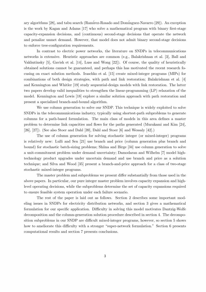
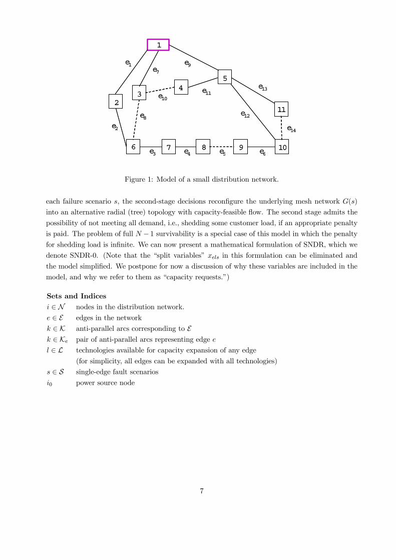
Figure 1 shows a model of a small distribution network. The solid and dashed lines represent

active and inactive edges, respectively. The active edges form the operating radial configuration in

which, for example, the power flow from node 1 to node 3 corresponds to flow on arc k = (1, 3) and

edge e7. A fault on e7 disconnects supply to node 3, and the radial configuration can be restored

and flow rerouted to this node by activating e10. (This fault would be isolated by opening switches,

not shown, located near the endpoints of e7.)

We can formulate the survivable network design problem as a two-stage stochastic program

with a scenario representation of uncertainty. The first stage determines capacity expansions. For

6

e1e7

e9

e1034

5

76

11

1098

2

e11e13

e2

e8

e4e3 e5 e6

e12

e14

1

e1e7

e9

e1034

5

76

11

1098

2

e11e13

e2

e8

e4e3 e5 e6

e12

e14

1

Figure 1: Model of a small distribution network.

each failure scenario s, the second-stage decisions reconfigure the underlying mesh network G(s)

into an alternative radial (tree) topology with capacity-feasible flow. The second stage admits the

possibility of not meeting all demand, i.e., shedding some customer load, if an appropriate penalty

is paid. The problem of full N − 1 survivability is a special case of this model in which the penaltyfor shedding load is infinite. We can now present a mathematical formulation of SNDR, which we

denote SNDR-0. (Note that the “split variables” xels in this formulation can be eliminated and

the model simplified. We postpone for now a discussion of why these variables are included in the

model, and why we refer to them as “capacity requests.”)

Sets and Indices

i ∈ N nodes in the distribution network.

e ∈ E edges in the network

k ∈ K anti-parallel arcs corresponding to Ek ∈ Ke pair of anti-parallel arcs representing edge e

l ∈ L technologies available for capacity expansion of any edge

(for simplicity, all edges can be expanded with all technologies)

s ∈ S single-edge fault scenarios

i0 power source node

7

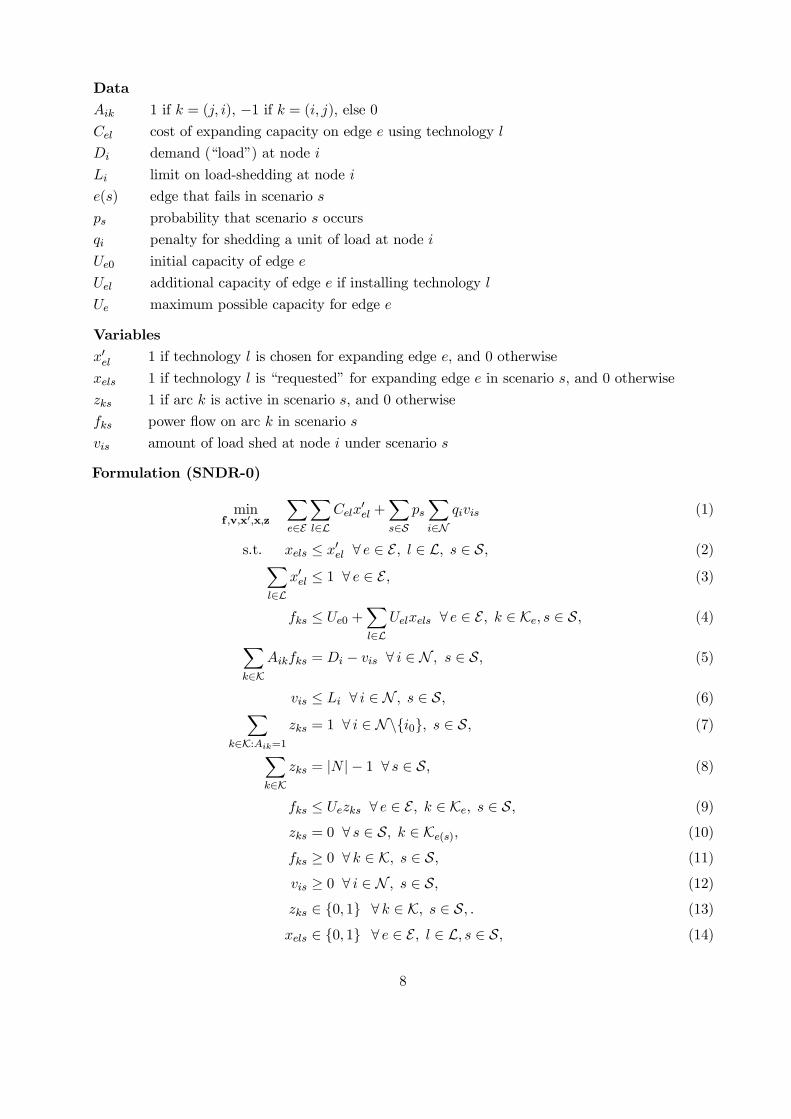
Data

Aik 1 if k = (j, i), −1 if k = (i, j), else 0Cel cost of expanding capacity on edge e using technology l

Di demand (“load”) at node i

Li limit on load-shedding at node i

e(s) edge that fails in scenario s

ps probability that scenario s occurs

qi penalty for shedding a unit of load at node i

Ue0 initial capacity of edge e

Uel additional capacity of edge e if installing technology l

Ue maximum possible capacity for edge e

Variables

x0el 1 if technology l is chosen for expanding edge e, and 0 otherwise

xels 1 if technology l is “requested” for expanding edge e in scenario s, and 0 otherwise

zks 1 if arc k is active in scenario s, and 0 otherwise

fks power flow on arc k in scenario s

vis amount of load shed at node i under scenario s

Formulation (SNDR-0)

minf ,v,x0,x,z

Xe∈E

Xl∈L

Celx0el +

Xs∈S

psXi∈N

qivis (1)

s.t. xels ≤ x0el ∀ e ∈ E, l ∈ L, s ∈ S, (2)Xl∈L

x0el ≤ 1 ∀ e ∈ E, (3)

fks ≤ Ue0 +Xl∈L

Uelxels ∀ e ∈ E, k ∈ Ke, s ∈ S, (4)Xk∈K

Aikfks = Di − vis ∀ i ∈ N , s ∈ S, (5)

vis ≤ Li ∀ i ∈ N , s ∈ S, (6)Xk∈K:Aik=1

zks = 1 ∀ i ∈ N\{i0}, s ∈ S, (7)

Xk∈K

zks = |N |− 1 ∀ s ∈ S, (8)

fks ≤ Uezks ∀ e ∈ E, k ∈ Ke, s ∈ S, (9)

zks = 0 ∀ s ∈ S, k ∈ Ke(s), (10)

fks ≥ 0 ∀ k ∈ K, s ∈ S, (11)

vis ≥ 0 ∀ i ∈ N , s ∈ S, (12)

zks ∈ {0, 1} ∀ k ∈ K, s ∈ S, . (13)

xels ∈ {0, 1} ∀ e ∈ E, l ∈ L, s ∈ S, (14)

8

x0el ∈ {0, 1} ∀ e ∈ E, l ∈ L. (15)

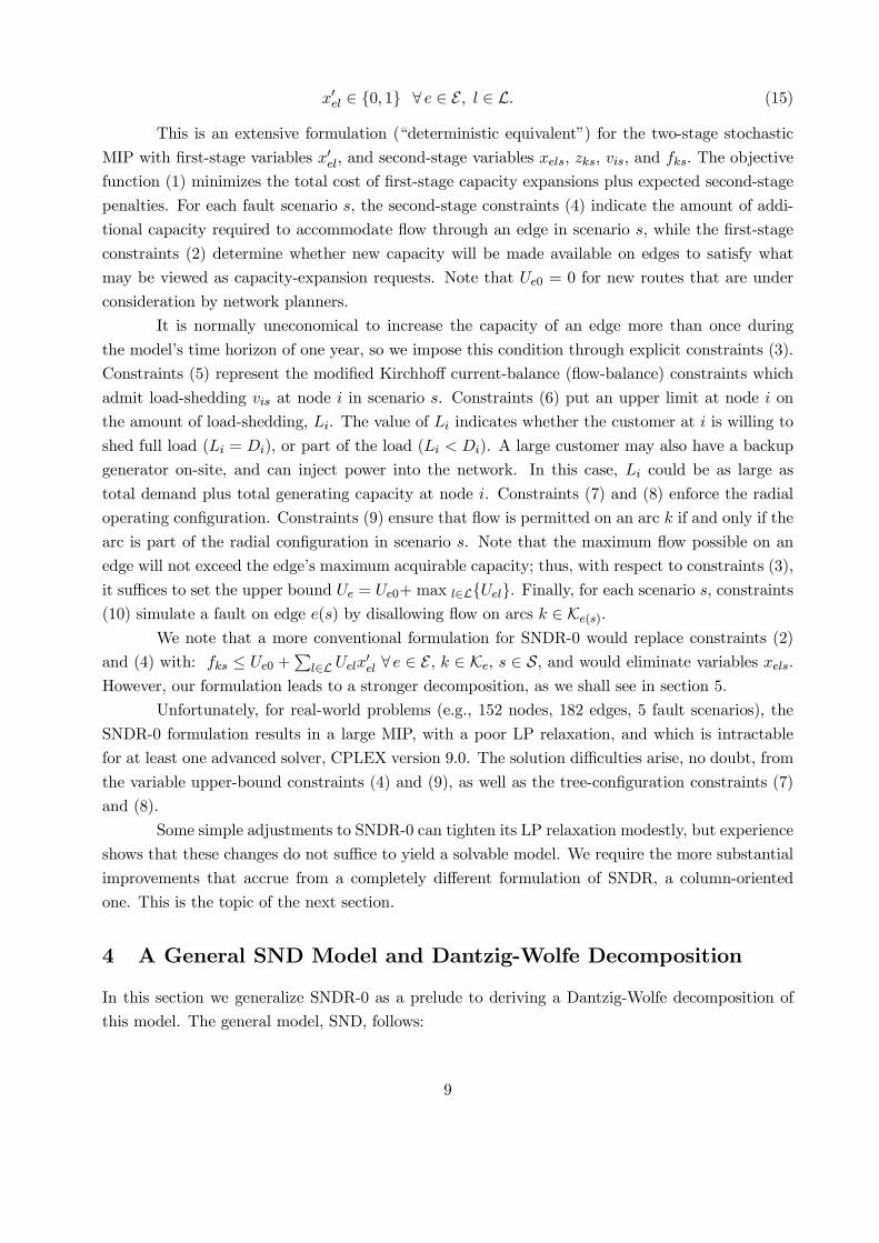
This is an extensive formulation (“deterministic equivalent”) for the two-stage stochastic

MIP with first-stage variables x0el, and second-stage variables xels, zks, vis, and fks. The objectivefunction (1) minimizes the total cost of first-stage capacity expansions plus expected second-stage

penalties. For each fault scenario s, the second-stage constraints (4) indicate the amount of addi-

tional capacity required to accommodate flow through an edge in scenario s, while the first-stage

constraints (2) determine whether new capacity will be made available on edges to satisfy what

may be viewed as capacity-expansion requests. Note that Ue0 = 0 for new routes that are under

consideration by network planners.

It is normally uneconomical to increase the capacity of an edge more than once during

the model’s time horizon of one year, so we impose this condition through explicit constraints (3).

Constraints (5) represent the modified Kirchhoff current-balance (flow-balance) constraints which

admit load-shedding vis at node i in scenario s. Constraints (6) put an upper limit at node i on

the amount of load-shedding, Li. The value of Li indicates whether the customer at i is willing to

shed full load (Li = Di), or part of the load (Li < Di). A large customer may also have a backup

generator on-site, and can inject power into the network. In this case, Li could be as large as

total demand plus total generating capacity at node i. Constraints (7) and (8) enforce the radial

operating configuration. Constraints (9) ensure that flow is permitted on an arc k if and only if the

arc is part of the radial configuration in scenario s. Note that the maximum flow possible on an

edge will not exceed the edge’s maximum acquirable capacity; thus, with respect to constraints (3),

it suffices to set the upper bound Ue = Ue0+ max l∈L{Uel}. Finally, for each scenario s, constraints(10) simulate a fault on edge e(s) by disallowing flow on arcs k ∈ Ke(s).

We note that a more conventional formulation for SNDR-0 would replace constraints (2)

and (4) with: fks ≤ Ue0 +Pl∈L Uelx

0el ∀ e ∈ E , k ∈ Ke, s ∈ S, and would eliminate variables xels.

However, our formulation leads to a stronger decomposition, as we shall see in section 5.

Unfortunately, for real-world problems (e.g., 152 nodes, 182 edges, 5 fault scenarios), the

SNDR-0 formulation results in a large MIP, with a poor LP relaxation, and which is intractable

for at least one advanced solver, CPLEX version 9.0. The solution difficulties arise, no doubt, from

the variable upper-bound constraints (4) and (9), as well as the tree-configuration constraints (7)

and (8).

Some simple adjustments to SNDR-0 can tighten its LP relaxation modestly, but experience

shows that these changes do not suffice to yield a solvable model. We require the more substantial

improvements that accrue from a completely different formulation of SNDR, a column-oriented

one. This is the topic of the next section.

4 A General SND Model and Dantzig-Wolfe Decomposition

In this section we generalize SNDR-0 as a prelude to deriving a Dantzig-Wolfe decomposition of

this model. The general model, SND, follows:

9

Data

c cost vector for expanding edge capacities

qs cost vector for operating the system under scenario s

u0 vector of initial edge capacities

Vs matrix that converts operating decisions and/or activities into edge-capacity

utilization under fault scenario s

U non-negative technology matrix that converts capacity-expansion decisions into available

operating capacity

Variables

x0 vector of binary decisions for capacity expansion of edges

xs vector of binary decisions indicating requests for capacity expansions that would ensure

feasible system operation under fault scenario s

ys vector of continuous and/or discrete operating decisions under fault scenario s

Ys set of feasible operating decisions under fault scenario s

Formulation (SND)

minx,y

c>x0 +Xs∈S

psq>s ys (16)

s.t. xs ≤ x0 ∀ s ∈ S, (17)

Vsys ≤ u0 + Uxs ∀ s ∈ S, (18)

ys ∈ Ys ∀ s ∈ S, (19)

xs ∈ {0, 1}|E||L| ∀ s ∈ S, (20)

x0 ∈ {0, 1}|E||L|. (21)

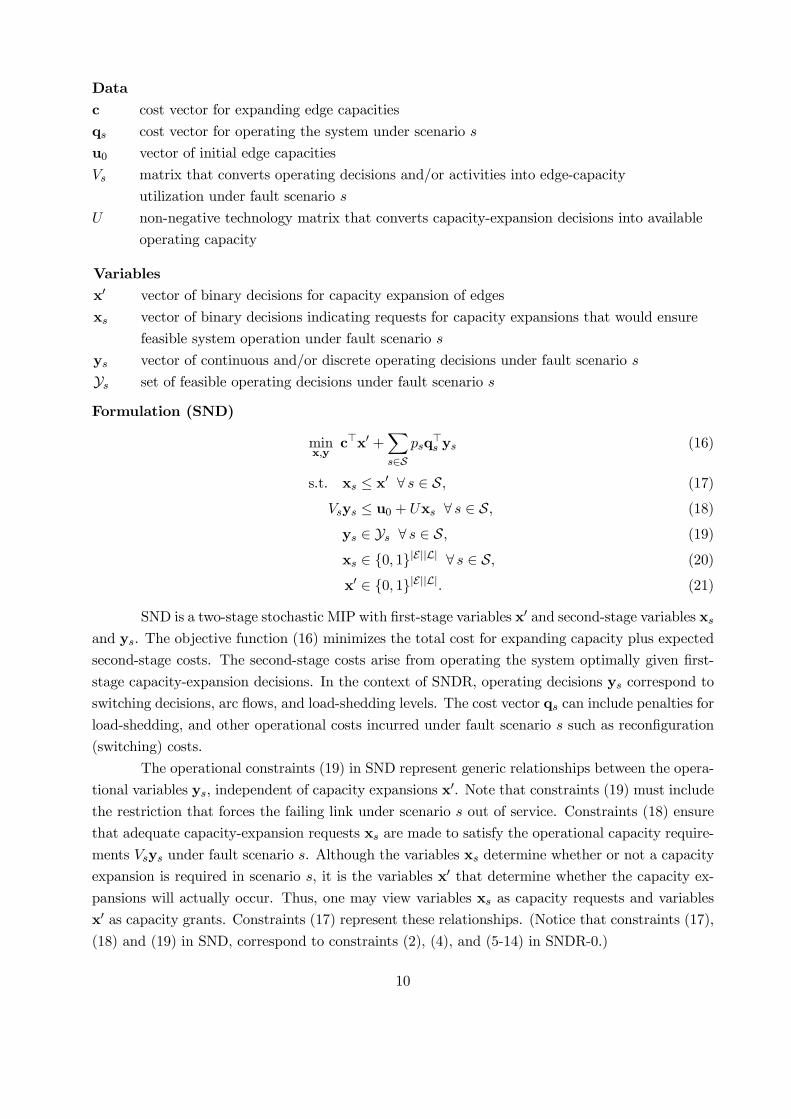
SND is a two-stage stochastic MIP with first-stage variables x0 and second-stage variables xsand ys. The objective function (16) minimizes the total cost for expanding capacity plus expected

second-stage costs. The second-stage costs arise from operating the system optimally given first-

stage capacity-expansion decisions. In the context of SNDR, operating decisions ys correspond to

switching decisions, arc flows, and load-shedding levels. The cost vector qs can include penalties for

load-shedding, and other operational costs incurred under fault scenario s such as reconfiguration

(switching) costs.

The operational constraints (19) in SND represent generic relationships between the opera-

tional variables ys, independent of capacity expansions x0. Note that constraints (19) must include

the restriction that forces the failing link under scenario s out of service. Constraints (18) ensure

that adequate capacity-expansion requests xs are made to satisfy the operational capacity require-

ments Vsys under fault scenario s. Although the variables xs determine whether or not a capacity

expansion is required in scenario s, it is the variables x0 that determine whether the capacity ex-pansions will actually occur. Thus, one may view variables xs as capacity requests and variables

x0 as capacity grants. Constraints (17) represent these relationships. (Notice that constraints (17),(18) and (19) in SND, correspond to constraints (2), (4), and (5-14) in SNDR-0.)

10

Observe that the inequality constraints (17) amount to nonanticipativity constraints over

the first-stage variables (Rockafellar and Wets [30]). Typically, nonanticipativity constraints equate

first-stage variables which have have been replicated by scenario. Inequalities, rather than equali-

ties, suffice in our case, however, because we assume that edge capacities cannot decrease.

Many SNDPs with sequential design, or with simultaneous design and global restoration,

will fit SND’s form. SNDR-0 ignores the non-failure state, so it may be viewed as sequential or

simultaneous design problem with global restoration. If the need arises for a strictly sequential

model with non-global restoration, we can simply modify u0 in constraints (18) to u0s in order

to represent initial capacity less the capacity consumed by baseline, non-failure flows that are

not disrupted in failure scenario s. The definition of Ys would also need to account for thatpart of the demand that is met by those undisrupted flows. Thus, the sequential-design models

in telecommunications, with link or path restoration, should fit the SND paradigm (e.g., [4, 19,

18]). Unfortunately, simultaneous design and non-global restoration may link subproblems with

continuous first-stage variables, and this would invalidate our proposed solution method.

We have seen that SND is general enough to accommodate many variants of survivable

network design. However, it may be impossible to solve realistically sized instances of the model

directly. To overcome this difficulty, we identify and exploit the special structure of SND using

Dantzig-Wolfe decomposition.

Constraints (18-20) are specific to fault scenario s. On the other hand, constraints (17)

link the capacity-expansion decisions across all fault scenarios. These constraints complicate the

structure of SND: without them the problem would separate into a set of small subproblems, one for

each fault scenario s. This motivates the use of a decomposition that partitions SND’s constraints

into two sets: linking (“complicating”) constraints (17), and constraints specific to scenario s. For

the latter constraints, we define

Xs =nxs | Vsys ≤ u0 +Uxs, xs ∈ {0, 1}|E||L|, ys ∈ Ys

o.

Letting Js denote the index set for Xs, i.e., Xs =nbxjs | j ∈ Jso, we can then express any

element of Xs through

xs =Xj∈Js

bxjswjs, Xj∈Js

wjs = 1, wjs ∈ {0, 1} ∀ j ∈ Js. (22)

Each element of Xs represents a set of capacity expansions (requests) that enable feasiblererouting of flows subject to network operational constraints under fault scenario s. We refer to

each such set of capacity expansions as a feasible expansion plan (FEP).

Without loss of generality, we assume that at least one optimal operational plan byjs is as-sociated with each FEP, i.e., Js simultaneously indexes FEPs and operational plans for scenario s.(For simplicity, we assume that MP is always feasible, i.e., Js 6= ∅ for all s.) Thus, attaching the op-erational costs q>s byjs to the wjs, and substituting expression (22) into SND yields its Dantzig-Wolfereformulation. (See Dantzig and Wolfe [8] as the seminal reference on Dantzig-Wolfe decompo-

sition for models with continuous variables, and see Appelgren [1] for the extension to integer

11

variables.) We denote this reformulated problem as the multi-scenario, column-oriented master

problem, “MP.” A detailed formulation follows. (“Dual variables” in the formulation correspond

to the model’s LP relaxation.)

Sets and Indices

j ∈ Js FEPs for fault scenario s

Databxjs binary vector representing capacity-expansion requests forming FEP j for fault scenario s

Variables

x0 binary decision vector for capacity expansion of edges

wjs 1 if FEP j is selected for fault scenario s, and 0 otherwise

Formulation (MP)

minx,w

c>x0+Xs∈S

Xj∈Js

psq>s byjswjs [dual variables] (23)

s.t.Xj∈Js

bxjswjs ≤ x0 ∀ s ∈ S, [πs] (24)

Xj∈Js

wjs = 1 ∀ s ∈ S, [μs] (25)

wjs ∈ {0, 1} ∀ s ∈ S, j ∈ Js (26)

x0 ∈ {0, 1}|E||L|. (27)

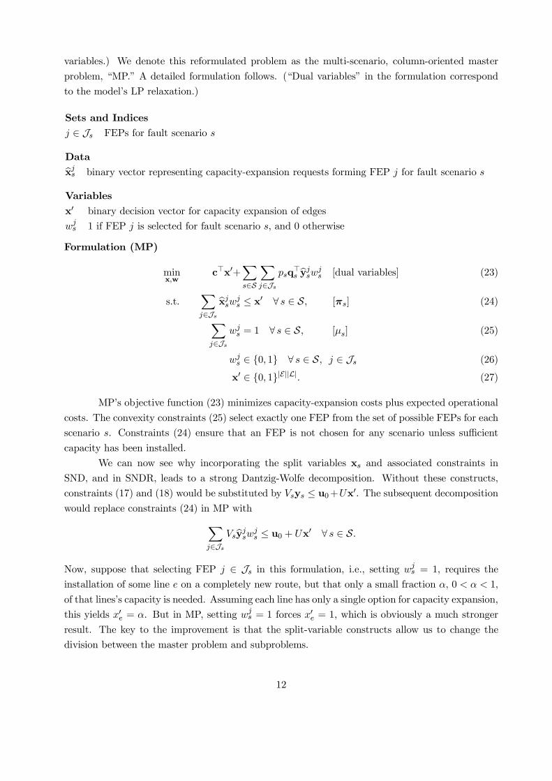
MP’s objective function (23) minimizes capacity-expansion costs plus expected operational

costs. The convexity constraints (25) select exactly one FEP from the set of possible FEPs for each

scenario s. Constraints (24) ensure that an FEP is not chosen for any scenario unless sufficient

capacity has been installed.

We can now see why incorporating the split variables xs and associated constraints in

SND, and in SNDR, leads to a strong Dantzig-Wolfe decomposition. Without these constructs,

constraints (17) and (18) would be substituted by Vsys ≤ u0+Ux0. The subsequent decompositionwould replace constraints (24) in MP withX

j∈JsVsbyjswjs ≤ u0 + Ux0 ∀ s ∈ S.

Now, suppose that selecting FEP j ∈ Js in this formulation, i.e., setting wjs = 1, requires the

installation of some line e on a completely new route, but that only a small fraction α, 0 < α < 1,

of that lines’s capacity is needed. Assuming each line has only a single option for capacity expansion,

this yields x0e = α. But in MP, setting wjs = 1 forces x0e = 1, which is obviously a much strongerresult. The key to the improvement is that the split-variable constructs allow us to change the

division between the master problem and subproblems.

12

It is impractical to solve MP by enumerating all possible columns (FEPs), so we employ

dynamic column generation: we generate columns “on the fly” through optimization subproblems.

To do this, we first create a restricted master problem (RMP) that contains only a modest-sized

subset of all the possible columns; Js now represents a working subset of columns for scenario s.The column-generation technique solves the LP relaxation of the RMP (RMP-LP) and

extracts the corresponding optimal dual variables bπs and bμs. The column-generation subproblemthen uses those values in an attempt to construct one or more “favorable” columns with a negative

reduced cost for the RMP; separate subproblems can be constructed for each scenario. If a favor-

able column is found, it is inserted into the RMP, which is then re-solved. The cycle of solving

subproblems and RMP-LP repeats until no favorable column can be identified. At that point, we

know that we have solved the LP relaxation of MP, and if that solution happens to be integer,

we have solved MP. If not, we may either resort to a branch-and-price algorithm, which generates

columns within a branch-and-bound procedure (Savelsbergh [32]), or settle for solving the RMP

as an IP in the hope of obtaining a good integer solution. (We refer the reader to Barnhart et al.

[2] for a comprehensive discussion of column generation, and to Lubbecke and Desrosiers [12] for a

compendium of column-generation applications.)

A column j for scenario s in MP has the form [psq>s byjs, bxjs, 1]>, where q>s byjs is the cost

of the associated operational plan byjs, and bxjs is the corresponding FEP. Given the optimal duals,bπs and bμs from RMP-LP, we can identify a column j having the most favorable reduced cost by

solving the subproblem

SP(s) minxs,ys

psq>s ys − bπ>s xs − bμs (28)

s.t. Vsys ≤ u0 + Uxs, (29)

ys ∈ Ys, (30)

xs ∈ {0, 1}|E||L|. (31)

Any solution (bxs, bys) of SP(s) with a negative objective value lets us create a new column for RMP,i.e., add a new element to Js. If no such solution exists for any s, then we have solved the LPrelaxation of the MP to optimality.

Each subproblem SP(s) is a deterministic network-design problem for a network lacking the

failed link, with operational constraints that depend on the application. (Of course, these subprob-

lems can accommodate simultaneous failures of links, which we do not need in our application.)

Thus, a subproblem may be strengthened and solved using methods that have been successful for

the specific application (e.g., Gunluk [10]).

We have successfully solved small problem instances of SNDR-0 using the column-generation

technique outlined. In almost every instance we obtain integer solutions from the optimized RMP-

LP, so we have not needed to implement a branch-and-price solution algorithm. But, a compu-

tational stumbling block does arise. For large, real-world problems, the subproblems SP(s) solve

quickly in early iterations of the solution algorithm, but much too slowly in later iterations. Other

researchers observe this effect as dual variables converge to their optimal values (Vanderbeck and

13

Wolsey [41]). To solve real-world problems, we must improve the solution times for SP(s), and to

do this we will exploit some of the special features of SNDR. This is the topic of the next section.

Some of the improvements require that load-shedding not be permitted, so we henceforth assume

that all variables vis are fixed to zero.

5 A Super-Network Formulation

This section describes a reformulation of the subproblems in the Dantzig-Wolfe decomposition of

SNDR to improve solvability. The constructs used will also strengthen the extensive formulation,

SNDR-0, so we describe them in this context. The next section then gives numerical results to

demonstrate empirical improvements.

It is logical in SNDR-0 to have variables that correspond to edges, but we will see here

that a more compact representation of the network and associated decision variables leads to a

tighter formulation. In particular, we exploit the sparse nature of the distribution network’s mesh

structure, the requirement that the network operate as a tree, and the assumption of no load-

shedding.

5.1 The Super-Network

Many nodes in a distribution network will have degree 2: we call these sub-nodes, and refer to

all nodes with degree 3 or greater as super-nodes. (All nodes with degree 1 have been recursively

collapsed into a sub-node or super-node.) LetM ⊆ N denote the set of all super-nodes. We say

that two super-nodes i and j are adjacent if they are joined by a chain in which all nodes except

i and j are sub-nodes. We denote this set of sub-nodes by Nij and let Eij denote the edges in thechain joining i and j. In the super-network, any chain joining two super-nodes i and j is represented

by two anti-parallel super-arcs k = (i, j) and k0 = (j, i). We say that the nodes in Nij and edgesin Eij are spanned by the super-arc k (or k0).

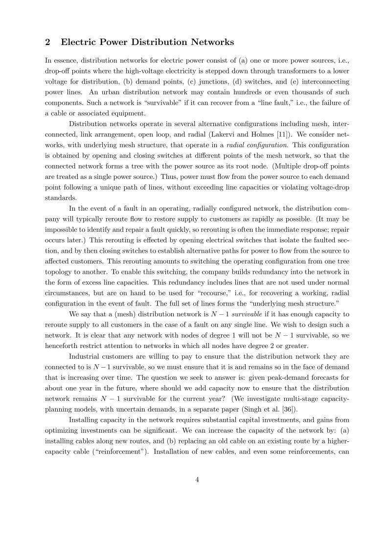
To illustrate, consider Figure 2(a) which extracts a small portion of the network in Figure

1 (in which M = {1, 3, 5, 6, 10}). That portion of the network contains super-nodes 6 and 10 forwhich E6,10 = {e3, e4, e5, e6} and N6,10 = {7, 8, 9}. Figure 2(b) shows the super-arcs k = (6, 10) andk0 = (10, 6) that span N6,10 and E6,10.

In SNDR-0, for a given scenario s, each edge e is represented by two flow variables, fks,

k ∈ Ke, two “tree variables” zks, k ∈ Ke, and one capacity-expansion variable xel for each l ∈ L.Thus, if |L| = 1 for all e ∈ E6,10 in Figure 2(a), 20 variables in SNDR-0 would result. In thesuper-network model below, SNDR-SN, will have one flow variable and one tree variable for each

super-arc, one capacity-expansion variable for each spanned edge and one “break-edge variable,”

described below, for each spanned edge. Thus, the portion of the super-network shown in Figure

2(b) requires only 12 variables.

To develop this model further, we restrict attention to the nontrivial case in which |Eij| > 1.Given a pair of adjacent super-nodes i and j, and a feasible radial configuration, we know that either:

14

)6,10(=′k

)10,6(=k

(a)

(b)

6 107 98e4e3 e5 e6

6 107 98e4e3 e5 e6

)6,10(=′k

)10,6(=k

(a)

(b)

6 107 98e4e3 e5 e67 98e4e3 e5 e6

6 107 98e4e3 e5 e6

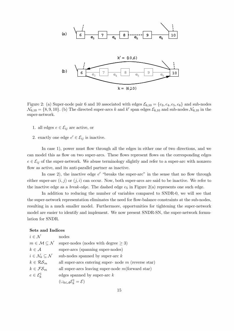
Figure 2: (a) Super-node pair 6 and 10 associated with edges E6,10 = {e3, e4, e5, e6} and sub-nodesN6,10 = {8, 9, 10}. (b) The directed super-arcs k and k0 span edges E6,10 and sub-nodes N6,10 in thesuper-network.

1. all edges e ∈ Eij are active, or

2. exactly one edge e0 ∈ Eij is inactive.

In case 1), power must flow through all the edges in either one of two directions, and we

can model this as flow on two super-arcs. These flows represent flows on the corresponding edges

e ∈ Eij of the super-network. We abuse terminology slightly and refer to a super-arc with nonzeroflow as active, and its anti-parallel partner as inactive.

In case 2), the inactive edge e0 “breaks the super-arc” in the sense that no flow througheither super-arc (i, j) or (j, i) can occur. Now, both super-arcs are said to be inactive. We refer to

the inactive edge as a break-edge. The dashed edge e5 in Figure 2(a) represents one such edge.

In addition to reducing the number of variables compared to SNDR-0, we will see that

the super-network representation eliminates the need for flow-balance constraints at the sub-nodes,

resulting in a much smaller model. Furthermore, opportunities for tightening the super-network

model are easier to identify and implement. We now present SNDR-SN, the super-network formu-

lation for SNDR.

Sets and Indices

i ∈ N nodes

m ∈M ⊆ N super-nodes (nodes with degree ≥ 3)k ∈ A super-arcs (spanning super-nodes)

i ∈ Nk ⊆ N sub-nodes spanned by super-arc k

k ∈ RSm all super-arcs entering super- node m (reverse star)

k ∈ FSm all super-arcs leaving super-node m(forward star)

e ∈ E1k edges spanned by super-arc k

(∪k∈AE1k = E)15

k ∈ A1 super-arc k, with (k + 1)st super-arc in anti-parallel

l ∈ L technologies for edges requiring expansion due to flows induced by

adjacent break-edges

e ∈ E2l set of edges that require expansion due to flow induced by an adjacent break-edge,

and such that technology l suffices for this expansion

e0 ∈ E3el set of edges which, when broken, induce flow on an edge e that requires it to

expand capacity if using technology l

i0 source node (always a super-node)

m(k) tail super-node of super-arc k

m(k) head super-node of super-arc k

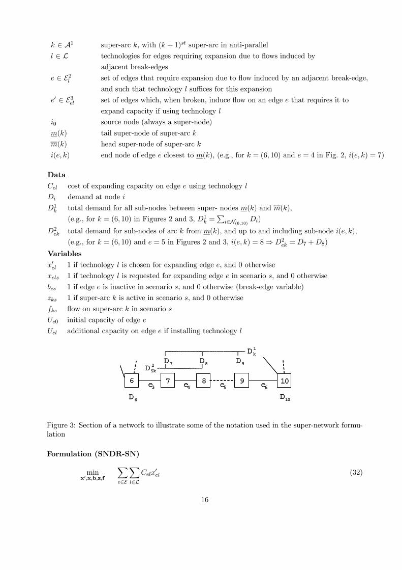
i(e, k) end node of edge e closest to m(k), (e.g., for k = (6, 10) and e = 4 in Fig. 2, i(e, k) = 7)

Data

Cel cost of expanding capacity on edge e using technology l

Di demand at node i

D1k total demand for all sub-nodes between super- nodes m(k) and m(k),

(e.g., for k = (6, 10) in Figures 2 and 3, D1k =Pi∈N(6,10) Di)

D2ek total demand for sub-nodes of arc k from m(k), and up to and including sub-node i(e, k),

(e.g., for k = (6, 10) and e = 5 in Figures 2 and 3, i(e, k) = 8⇒ D2ek = D7 +D8)

Variables

x0el 1 if technology l is chosen for expanding edge e, and 0 otherwise

xels 1 if technology l is requested for expanding edge e in scenario s, and 0 otherwise

bes 1 if edge e is inactive in scenario s, and 0 otherwise (break-edge variable)

zks 1 if super-arc k is active in scenario s, and 0 otherwise

fks flow on super-arc k in scenario s

Ue0 initial capacity of edge e

Uel additional capacity on edge e if installing technology l

76 1098e4e3 e5 e6

6D 10D

1kD

7D 8D 9D25kD

76 1098e4e3 e5 e6

6D 10D

1kD

7D 8D 9D25kD

Figure 3: Section of a network to illustrate some of the notation used in the super-network formu-lation

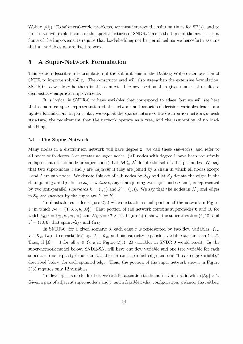
Formulation (SNDR-SN)

minx0,x,b,z,f

Xe∈E

Xl∈L

Celx0el (32)

16

s.t Capacity-expansion constraints

xels ≤ x0el, ∀ e ∈ E, l ∈ L, s ∈ S, (33)

At most one expansion for each edge:Xl∈L

x0el ≤ 1 ∀ e ∈ E, (34)

Super-arc flow capacity-expansion constraints:

fks −D2ekzks ≤ Ue0zks +Xl∈L

Uelxels ∀k ∈ A, e ∈ E1ks ∈ S, (35)

Flow-balance constraints:Xk∈RSm

(fks −D1kzks)−X

k∈FSmfks −

Xk∈FSm

Xe∈E1k

D2ekbes

= Dm ∀ s ∈ S, m ∈M\{i0}, (36)

Exactly one edge spanned by a super-arc is broken or all edges are active:

zks + zk+1,s +Xe∈E1k

bes = 1 ∀k ∈ A1, s ∈ S, (37)

Flow in tree (feasible configuration):

fks ≤ Ukzks ∀ k ∈ A, s ∈ S, where Uk = mine∈E1k©D2ek + Ue0 + maxl∈L Uel

ª, (38)

Tree constraint 1:Xk∈A

zks = |M|− 1 ∀ s ∈ S, (39)

Tree constraint 2:Xk∈RSm

zks = 1 ∀m ∈M\{i0}, s ∈ S, (40)

Fault-simulation constraints:

be(s)s = 1 ∀ s ∈ S, (41)

Domain restrictions on variables:

fks ≥ 0 ∀ k ∈ A, s ∈ S, (42)

bes ∈ {0, 1} ∀ e ∈ E, s ∈ S, (43)

xel ∈ {0, 1} ∀ e ∈ E, l ∈ L, (44)

zks ∈ {0, 1} ∀k ∈ A, s ∈ S. (45)

The objective function (32) minimizes the total cost of capacity expansion. Similar to SNDR-0,

constraints (33) determine whether new capacity will be made available on an edge, and constraints

(34) allow at most one capacity expansion on any edge.

This formulation does not explicitly model flows on the edges (or arcs). Instead, we derive

them from super-arc flows fks. To be more precise, the flow on the first edge that a super-arc spans

equals the super-arc flow fks. For super-arcs that span more than one edge, the flow on each edge

17

is calculated by subtracting the upstream demand D2ek from the super-arc flow fks; this is shown

on the left-hand-side of the super-arc capacity-expansion constraints (35). This forces expansion

on an edge if the edge flow exceeds its initial capacity Ue0.

For each fault scenario s, constraint (41) simulates a fault on edge e(s) by forcing it to be

inactive (i.e., by making it a break-edge). Constraints (37) and (38) ensure that when a break-edge

e breaks a super-arc k (bes = 1), the corresponding super-arc flow is zero. Furthermore, constraints

(37) ensure that at most one active super-arc exists between any pair of super-nodes, and that no

break-edge is defined if the super-arc is active.

SNDR-SN enforces flow-balance constraints (36) only at super-nodes. These constraints

have an extra “flow-out” termPk∈FSm

Pe∈E1k D

2ekbes, which constitutes the flow needed to satisfy

demand of sub-nodes up to the break-edge on each inactive (“broken”) super-arc k ∈ FSm.Constraints (39) and (40) ensure that the super-network satisfies the radial-configuration

requirement by forcing the set of active super-arcs (zks = 1) to form a “super-tree.” As with flow-

balance constraints, constraints (40) are only defined for super-nodes in SNDR-SN, which means

that fewer of these configuration constraints appear in SNDR-SN compared to SNDR-0.

5.2 Strengthening the Super-Network Formulation

Since the super-network formulation aggregates electricity demand into super-nodes, it cannot, in

general, be applied to problems with load-shedding penalties that vary by node. However, under the

realistic setting of no load-shedding, we can strengthen the super-network formulation by adding

extra constraints that take advantage of lower bounds on the power flows in the arcs.

First observe that if¯E1k ¯ > 1 and a break-edge e breaks a super-arc k, then fks = 0, but

(implicit) flow on edges e ∈ E1k\{e} is likely to occur. Thus, we can apply a preprocessing step thatadds a “break-edge expansion constraint” when a break in edge e ∈ E1k results in flow on an edgee ∈ E1k that exceeds that edge’s initial capacity Ue0. These constraints force an expansion on edge ewhen there is a break on edge e. In some instances when

¯E1k ¯ > 2, breaks in several different edgese ∈ E1k may result in the creation of several break-edge expansion constraints for the same adjacentedge e ∈ E1k . In such cases, it is possible to combine these to give a constraint of the following form:X

e0∈E3elbe0s ≤ xels ∀ l ∈ L, e ∈ E2l , s ∈ S. (46)

We may also strengthen the model by bounding the flow on a super-arc if it is used. For

example, if super-arc k is active, then the minimum flow fks (which leaves m(k)) is bounded below

by D1k +Dm(k), i.e., the total demand for all sub-nodes in Nk plus the demand at the head nodem(k) of super-arc k. We use this information to impose lower-bounding constraints such as:

fks ≥ (D1k +Dm(k))zks ∀ s ∈ S, k ∈ A. (47)

We also use this information to compute the minimum required flow through the edge e ∈E1k if super-arc k is used, and define capacity-expansion constraints that force expansions on edges

18

e if their flow exceeds their initial capacities Ue0. Such constraints are defined by:

zks ≤Xl∈L

xel ∀s ∈ S, k ∈ A2, e ∈ E4k , (48)

where the set A2 represents super-arcs k which, when active, result in flow that forces expansionon edges e ∈ E1k , and where the set E4k denotes edges e ∈ E1k requiring expansion if super-arc k ∈A2 is active.

Additional improvements in the LP relaxation are made by multiplying the coefficients D2ekand Ue0 by zks in the capacity-expansion constraints (35). (Constraints (2) in SNDR-0 can also be

strengthened by multiplying Ue0 with zks, but this does not improve performance significantly.)

6 Computational Experiments

This section demonstrates the relative computational performance of the models and solution pro-

cedures described above. All problem instances derive from data for a distribution network in New

Zealand. The network supplies power to an urban area that contains mostly large industrial and

commercial customers who pay extra fees for a high level of reliability, i.e., for an N − 1 survivablenetwork. Peak-demand data has been forecasted one year forward.

The network data comprise 152 nodes, most of which are demand points, and 182 edges.

Four demand points represent completely new demand, and 14 edges represent new cable routes. We

model a single capacity-expansion technology for each edge and consider single-line fault scenarios.

The super-network representation of this problem has only 32 super-nodes and 124 super-arcs. For

testing, a set of problem instances is obtained by varying the number of fault scenarios. We model

potential faults on only 179 of the 182 lines because three lines supply large customers who have

dedicated backup lines.

Computational tests are carried out on a desktop computer with a 2.6 GHz Pentium IV

processor and 1 GB of RAM. We generate all models, and implement our decomposition algorithms

within the Mosel algebraic modeling system, version 1.24, from Dash Optimization. RMP-LP is

solved with Xpress-MP, version 14.24, also from Dash Optimization, but the MIP subproblems and

the extensive-form problems are solved with CPLEX, version 9.0 from ILOG, Inc.

With two exceptions, solver parameters are fixed at default values throughout all tests.

The exceptions involve CPLEX: Gomory cuts are turned off, and a moderate level of probing

is used (CPX PARAM PROBE = 2). All MIP subproblems are solved to optimality, while the

extensive-form problems are solved with a relative optimality tolerance of 0.05%.

Observe that any instance of RMP-LP will be infeasible unless one feasible column (FEP)

exists for each fault scenario. We could use a “Phase I approach” for finding an initial feasible

solution (e.g., Dantzig and Thapa [9], pp. 291-292), but it is simpler to guarantee such a solution

by seeding the master problem with one FEP for each fault scenario. Except for trivially infeasible

problems, an FEP that requires all possible capacity expansions will surely be feasible for any

scenario, so those define our initial columns. Our application imposes no operational costs, so

these initial columns, as well as columns generated later, have cost coefficients of 0.

19

At each iteration of the decomposition algorithm, we can readily obtain a lower bound on

the optimal objective value for MP-LP (see Wolsey [43], p. 189) and thereby bound the optimality

gap for this LP relaxation. In practice, we solve RMP-LP until this gap drops below 0.05% and

then check to see if the current solution is integral. If it is–and it usually is–we have obtained

an integer solution to SNDR-0 that is within 0.05% of optimality and can halt. If not, we enforce

the integer restrictions in the RMP and solve it by branch and bound. We cannot guarantee that

a good integer solution will be obtained this way, but the worst optimality gap we have observed

is 1.3%.

Our master problems suffer from severe dual degeneracy. Consequently, convergence using a

conventional Dantzig-Wolfe algorithm is slow, ranging from hours to days. To improve convergence,

we apply “duals stabilization” in the RMP-LP, and compare two different methods: du Merle et

al. [13] describe the first, which we call “du Merle duals stabilization”; the other method simply

generates interior-point dual solutions by solving RMP-LP using an interior-point algorithm. We

call this technique “interior-point duals stabilization.”

The following abbreviations denote the formulations discussed in earlier sections.

SNDR-0 the original formulation, solved in extensive form

SNDR-SN the super-network formulation, solved in extensive form

SNDR-SNS SNDR-SN with strengthening as described in section 5

CG-0 column generation with du Merle duals stabilization, using subproblems

derived from SNDR-0

CG-SNS column generation with du Merle duals stabilization, using subproblems

derived from SNDR-SNS

CG-SNS-I column generation with interior-point duals stabilization, using subproblems

derived from SNDR-SNS

Table 1 displays the solution times for 14 problem instances. We attempt to solve each

instance with the six solution approaches outlined above. The results summarize easily: the super-

network model for SNDR, SNDR-SN, is faster than the original model SNDR-0, and the strength-

ened super-network model SNDR-SNS is faster yet. Column generation with interior-point duals

stabilization and strengthened super-network subproblems (CG-SNS-I) is vastly more efficient than

the other solution methods.

The results listed under CG-0 and CG-SNS show that the strengthened super-network con-

structs contribute substantially to efficiency. Just as critical is the use of the interior-point duals

stabilization, which significantly outperforms the du Merle alternative. For instance, experimenta-

tion with the 50-fault instance reveals that CG-SNS (du Merle) requires 36,000 seconds to reach a

relative optimality gap of 7.6%, while CG-SNS-I which reaches a gap of 5.3% in only 1,200 seconds.

It is interesting to compare the optimal objective values for the LP relaxations of the ex-

tensive formulations, and the optimal objective value for MP-LP. For the 4-fault instance, these

values for SNDR-0, SNDR-SN, SNDR-SNS , and the Dantzig-Wolfe master problems, are 112008,

117429, 222472, and 893686, respectively. These results clearly show that the super-network for-

mulation substantially improves upon the LP relaxation of the original model, and shows that the

20

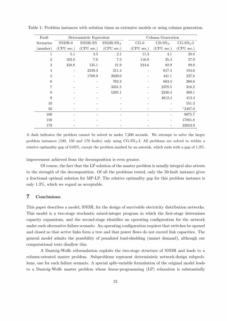
Table 1: Problem instances with solution times as extensive models or using column generation.

Fault Deterministic Equivalent Column Generation

Scenarios SNDR-0 SNDR-SN SNDR-SNS CG-0 CD-SNS CG-SN5-I

(number) (CPU sec.) (CPU sec.) (CPU sec.) (CPU sec.) (CPU sec.) (CPU sec.)

1 5.1 4.5 2.1 11.3 4.1 28.8

2 102.8 7.6 7.5 116.9 35.4 57.9

3 458.8 135.1 21.9 224.6 92.9 89.0

4 - 2249.3 211.4 - 617.4 184.6

5 - 1789.9 2039.0 - 441.1 237.8

6 - - 762.3 - 683.4 260.6

7 - - 3331.5 - 2378.5 316.2

8 - - 5285.1 - 2240.4 389.1

9 - - - - 4612.4 413.4

10 - - - - - 551.3

50 - - - - - ∗2487.0100 - - - - - 9075.7

150 - - - - - 17881.8

179 - - - - - 22653.9

A dash indicates the problem cannot be solved in under 7,200 seconds. We attempt to solve the larger

problem instances (100, 150 and 179 faults) only using CG-SNS-I. All problems are solved to within a

relative optimality gap of 0.05%, except the problem marked by an asterisk, which ends with a gap of 1.3%.

improvement achieved from the decomposition is even greater.

Of course, the fact that the LP solution of the master problem is usually integral also attests

to the strength of the decomposition. Of all the problems tested, only the 50-fault instance gives

a fractional optimal solution for MP-LP. The relative optimality gap for this problem instance is

only 1.3%, which we regard as acceptable.

7 Conclusions

This paper describes a model, SNDR, for the design of survivable electricity distribution networks.

This model is a two-stage stochastic mixed-integer program in which the first-stage determines

capacity expansions, and the second-stage identifies an operating configuration for the network

under each alternative failure scenario. An operating configuration requires that switches be opened

and closed so that active links form a tree and that power flows do not exceed link capacities. The

general model admits the possibility of penalized load-shedding (unmet demand), although our

computational tests disallow this.

A Dantzig-Wolfe reformulation exploits the two-stage structure of SNDR and leads to a

column-oriented master problem. Subproblems represent deterministic network-design subprob-

lems, one for each failure scenario. A special split-variable formulation of the original model leads

to a Dantzig-Wolfe master problem whose linear-programming (LP) relaxation is substantially

21

stronger than that of the extensive formulation.

The effectiveness of the column-generation procedure for solving SNDR relies heavily on

modeling improvements that strengthen the formulation of the subproblems. These improvements

involve modeling the network structure through a condensed construct, a “super-network,” which

leads to smaller subproblems with tighter LP relaxations. This super-network then reveals further

opportunities for tightening the model.

The use of a good duals-stabilization scheme for the master problem is essential for the

efficiency of the column-generation solution procedure. Our results show that simply using interior-

point duals (“interior-point duals stabilization”) greatly outperforms the well-known scheme of du

Merle et al. [13].

Looking forward, our modeling and solution approach can be applied to other design prob-

lems for survivable networks in telecommunications, logistics and electric-power transmission. It

will be interesting to see if similar or better computational results can be achieved using these

techniques in other industries.

References

[1] Appelgren, L.H., 1969, “A column generation algorithm for a ship scheduling problem,” Trans.

Sci., 3, pp. 53—68.

[2] Barnhart, C., Johnson, E.L., Nemhauser, G.L., Savelsbergh, M.W.P., Vance, P.H., 1998,

“Branch-and-price: Column generation for solving huge integer programs,” Oper. Res., 46,

pp. 316—329.

[3] Balakrishnan, A., Magnanti, T.L., Sokol, J.S., Wang, Y., 2001, “Telecommunication link

restoration planning with multiple facility types,” Annals of Oper. Res., 106, pp. 127—154.

[4] Balakrishnan, A., Magnanti, T.L., Sokol, J.S., Wang, Y., 2002, “Spare-capacity assignment

for line restoration using a single-facility type,” Oper. Res., 50, pp. 617—635.

[5] Ball, M.O., Vakhutinsky, A., 2001, “Fault-tolerant virtual path layout in ATM networks,”

INFORMS J. Comput., 13, pp. 76—94.

[6] Dahl, G., Stoer, M., 1998, “A cutting plane algorithm for multicommodity survivable network

design problems,” INFORMS J. Comput., 10, pp. 1—11.

[7] Damodaran, P., Wilhelm, W., 2004, “Branch-and-price methods for prescribing profitable

upgrades of high-technology products with stochastic demands,” Dec. Sci., 35, pp. 55—81.

[8] Dantzig, G.B., Wolfe, P., 1960, “Decomposition principle for linear programs,” Oper. Res., 8,

pp. 101—111.

[9] Dantzig, G.B., Thapa, M.N., 2003, Linear Programming. 2: Theory and Extensions, Springer

Series in Operations Research, Springer-Verlag, New York.

22

[10] Gunluk, O., 1999, “A branch-and-cut algorithm for capacitated network design problems,”

Math. Prog., 86, pp. 17—39.

[11] Lakervi, E., Holmes, E.J., 1995, Electricity Distribution Network Design, Peter Peregrinus,

Ltd., London.

[12] Lubbecke, M.E., Desrosiers, J., 2002, “Selected topics in column generation,” Les Cahiers de

GERAD G-2002-64, Group for Research in Decision Analysis, Montreal, Canada.

[13] du Merle, O., Villeneuve, D., Desrosiers, J., Hansen, P., 1999, “Stabilized column generation,”

Discrete Math., 194, 229—237.

[14] Gavish, B., Trudeau, P., Dror, M., Gendreau, M., Mason, L., 1989, “Fiberoptic circuit network

design under reliability constraints,” IEEE J. on Selected Areas in Comm., 7, pp. 1181—1187.

[15] Iraschko, R.R., MacGregor, M.H., Grover, W.D., 1998, “Optimal capacity placement for path

restoration in STM or ATM mesh-survivable networks,” IEEE/ACM Trans. Net., 6, pp. 325—

336.

[16] Johnson, D.S., Lenstra, J.K., Rinnooy Kan, A.H.G., 1978, “The complexity of the network

design problem ,” Networks, 8, pp. 279—285.

[17] Kagan, N., Adams, R. N., 1993, “A benders decomposition approach to the multi-objective

distribution planning problem,” Int. J. Elec. Power & Energy Systems, 15, pp. 259—271.

[18] Kennington, J.L., Lewis, M.W., 2001, “The path restoration version of the spare capacity allo-

cation problem with modularity restrictions: Models, algorithms, and an empirical analysis,”

INFORMS J. Comput., 13, pp. 181—190.

[19] Kennington, J.L., Whitler, J.E., 1999, “An efficient decomposition algorithm to optimize spare

capacity in a telecommunications network,” INFORMS J. Comput., 11, pp. 149—160.

[20] Kuwabara, H., Nara, K., 1997, “Multi-year and multi-state distribution systems expansion

planning by multi-stage branch exchange,” IEEE Trans. on Power Delivery, 12, pp. 457—463.

[21] Lulli, G., Sen, S., 2004, “A branch-and-price algorithm for multistage stochastic integer pro-

gramming with application to stochastic batch-sizing problems,” Manage. Sci., 50, pp. 786—

796.

[22] Luss, H., Wong, R.T., 2004, “Survivable telecommunications network design under different

types of failures,” IEEE Trans. on Systems, Man, and Cybernetics-Part A: Systems and Hu-

mans, 34, pp. 521—530.

[23] Magnanti, T.L., Wolsey, L.A., 1995, “Design of survivable networks,” in Handbook in Op-

erations Research and Management Science, Volume 7: Network Models M.O. Ball, T.L.

Magnanti, C.L. Monma and G.L. Nemhauser eds., Elsevier Publishing Co., Amsterdam, pp.

503—616.

23

[24] Murakami, K., Kim, H.S., 1998, “Optimal capacity and flow assignment for self-healing ATM

networks based on line and end-to-end restoration,” IEEE/ACM Trans. Net., 6, pp. 207—221.

[25] Nara, K., Kuwabara, H., Kitagawa, M., Ohtaka, K., 1994, “Algorithm for expansion planning

in distributions systems taking faults into consideration,” IEEE Trans. Power Syst., 9, pp.

324—330.

[26] Rajan, D., Atamturk, A., 2002, “Survivable network design: Routing of flows and slacks,” in

Telecommunications Network Design and Management, G. Anandalingam and S. Raghavan,

eds., Kluwer Academic Publishers, New York, pp. 65—81, 2002.

[27] Rajan, S., Atamturk, A., 2004, “A directed cycle-based column-and-cut generation method

for capacitated survivable network design,” Networks, 43, pp. 201—211.

[28] Ramiirez-Rosado, I.J., Bernal-Agustin, J.L., 2001, “Reliability and costs optimization for dis-

tribution networks expansion using an evolutionary algorithm,” IEEE Trans. Power Syst., 16,

pp. 111—118.

[29] Ramirez-Rosado, I.J., Dominguez-Navarro, J.A., 2004, “Possibilistic model based on fuzzy sets

for the multiobjective optimal planning of electric power distribution networks,” IEEE Trans.

Power Syst., 19, pp. 1801—1810.

[30] Rockafellar R. and Wets, R.J.-B., 1991, “Scenarios and policy aggregation in optimization

under uncertainty,” Math. Oper. Res., 6, pp. 119—147.

[31] Samarakoon, H., Shrestha, R. and Fujiwara, O., 2001, “A mixed integer linear programming

model for transmission expansion planning with generation location selection, Int. J. of Elec-

trical Power & Energy Systems, 23, pp. 285—293.

[32] Savelsbergh, M., 1997, “Branch and price algorithm for generalised assignment problem,”

Oper. Res., 35, pp. 442—456.

[33] Schultz, R., Stougie, L., van der Vlerk, M.H., 1996, “Two-stage stochastic integer program-

ming: A survey,” Statistica Neerlandica, 50, pp. 404—416.

[34] Shiina, T., Birge, J.R., 2004, “Stochastic unit commitment problem,” Int. Trans. Oper. Res.,

11, pp. 19—32.

[35] Silva, E.F., Wood, R.K., 2004, “Solving a class of stochastic mixed-integer programs by branch-

and-price,” Math. Prog. (Series B), 108, pp. 395—418.

[36] Singh, K., Philpott, A., Wood, K., 2007, “Dantzig-Wolfe decomposition for solving multi-stage

stochastic capacity-planning problems,” Working paper, Department of Engineering Science,

University of Auckland.

[37] Snyder, L., Daskin, M., 2004, “Reliability models for facility location: The expected failure

cost case,” ISE Technical Report #04T-016, Lehigh University, Bethlehem, Pennsylvania.

24

[38] Soni, S., Gupta, R., Pirkul, H., 1999, “Survivable network design: The state of the art,”

Information Systems Frontiers, 1, pp. 303—315.

[39] Stoer, M., Dahl, G., 1994, “A polyhedral approach to multicommodity survivable network

design,” Numerische Mathematik, 68, pp. 149—167.

[40] Thadakamalla, H., Raghavan, U., Kumara, S., Albert, R., 2004, “Survivability of multiagent-

based supply networks: A topological perspective,” IEEE Intelligent Syst., 19, pp. 24—31.

[41] Vanderbeck, F., Wolsey, L.A., 1996, “An Exact Algorithm for IP Column Generation,” Oper.

Res. Letters, 19, 151—159.

[42] Wessaly, R., 2000, “Dimensioning survivable capacitated networks,” PhD thesis, Technische

Universitat Berlin, April.

[43] Wolsey, L.A., 1998, Integer Programming, John Wiley & Sons, New York.

[44] Wood, A., Wollenberg, B., 1996, Power Generation, Operation and Control, Second Edition,

John Wiley & Sons, New York.

[45] Xiong, Y., Mason, L.G., 1999, “Restoration strategies and spare capacity requirements in

self-healing ATM networks,” IEEE/ACM Trans. Net., 7, pp. 98—110.

25