KATARA: A Data Cleaning System Powered by KnowledgeBases and Crowdsourcing

Xu Chu1∗ John Morcos1∗ Ihab F. Ilyas1∗

Mourad Ouzzani2 Paolo Papotti2 Nan Tang2 Yin Ye2

1University of Waterloo 2Qatar Computing Research Institute{x4chu,jmorcos,ilyas}@uwaterloo.ca {mouzzani,ppapotti,ntang,yye}@qf.org.qa

ABSTRACTClassical approaches to clean data have relied on using in-tegrity constraints, statistics, or machine learning. Theseapproaches are known to be limited in the cleaning accu-racy, which can usually be improved by consulting masterdata and involving experts to resolve ambiguity. The adventof knowledge bases (kbs), both general-purpose and withinenterprises, and crowdsourcing marketplaces are providingyet more opportunities to achieve higher accuracy at a largerscale. We propose Katara, a knowledge base and crowdpowered data cleaning system that, given a table, a kb, anda crowd, interprets table semantics to align it with the kb,identifies correct and incorrect data, and generates top-kpossible repairs for incorrect data. Experiments show thatKatara can be applied to various datasets and kbs, andcan efficiently annotate data and suggest possible repairs.

1. INTRODUCTIONA plethora of data cleaning approaches that are based on

integrity constraints [2,7,9,20,36], statistics [30], or machinelearning [43], have been proposed in the past. Unfortunately,despite their applicability and generality, they are best-effortapproaches that cannot ensure the accuracy of the repaireddata. Due to their very nature, these methods do not haveenough evidence to precisely identify and update errors. Forexample, consider the table of soccer players in Fig. 1 and afunctional dependency B → C, which states that B (coun-try) uniquely determines C (capital). This would identify aproblem for the four values in tuple t1 and t3 over the at-tributes B and C. A repair algorithm would have to guesswhich value to change so as to “clean” the data.

To increase the accuracy of such methods, a natural ap-proach is to use external information in tabular masterdata [19] and domain experts [19,35,40,44]. However, theseresources may be scarce and are usually expensive to em-ploy. Fortunately, we are witnessing an increased availabil-ity of both general purpose knowledge bases (kbs) such as

∗Work partially done while interning/working at QCRI.

Permission to make digital or hard copies of all or part of this work for personal orclassroom use is granted without fee provided that copies are not made or distributedfor profit or commercial advantage and that copies bear this notice and the full cita-tion on the first page. Copyrights for components of this work owned by others thanACM must be honored. Abstracting with credit is permitted. To copy otherwise, or re-publish, to post on servers or to redistribute to lists, requires prior specific permissionand/or a fee. Request permissions from Permissions@acm.org.SIGMOD’15, May 31–June 4, 2015, Melbourne, Victoria, Australia.Copyright c© 2015 ACM 978-1-4503-2758-9/15/05 ...$15.00.http://dx.doi.org/10.1145/2723372.2749431.

Al B C D E F Gbt1 Rossi Italy Rome Verona Italian Proto 1.78bt2 Klate S. Africa Pretoria Pirates Afrikaans P. Eliz. 1.69bt3 Pirlo Italy Madrid Juve Italian Flero 1.77

Figure 1: A table T for soccer players

Yago [21], DBpedia [31], and Freebase, as well as special-purpose kbs such as RxNorm1. There is also a sustainedeffort in the industry to build kbs [14]. These kbs are usu-ally well curated and cover a large portion of the data athand. In addition, while access to an expert may be limitedand expensive, crowdsourcing has been proven to be a viableand cost-effective alternative solution.

Challenges. Effectively exploring kbs and crowd in datacleaning raises several new challenges.

(i) Matching (dirty) tables to kbs is a hard problem. Tablesmay lack reliable, comprehensible labels, thus requiring thematching to be executed on the data values. This may leadto ambiguity; more than one mapping may be possible. Forexample, Rome could be either city, capital, or club in thekb. Moreover, tables usually contain errors. This wouldtrigger problems such as erroneous matching, which will adduncertainty to or even mislead the matching process.

(ii) kbs are usually incomplete in terms of the coverage ofvalues in the table, making it hard to find correct table pat-terns and associate kb values. Since we consider data thatcould be dirty, it is often unclear, in the case of failing tofind a match, whether the database values are erroneous orthe kb does not cover these values.

(iii) Human involvement is needed to validate matchings andto verify data when the kbs do not have enough coverage.Effectively involving the crowd requires dealing with tradi-tional crowdsourcing issues such as forming easy-to-answerquestions for the new data cleaning tasks and optimizing theorder of issuing questions to reduce monetary cost.

Despite several approaches for understanding tables withkbs [13,28,39], to the best of our knowledge, they do not ex-plicitly assume the presence of dirty data. Moreover, previ-ous work exploiting reference information for repair has onlyconsidered full matches between the tables and the masterdata [19]. On the contrary, with kbs, partial matches arecommon due to the incompleteness of the reference.

To this end, we present Katara, the first data cleaningsystem that leverages prevalent trustworthy kbs and crowd-sourcing for data cleaning. Given a dirty table and a kb,

1https://www.nlm.nih.gov/research/umls/rxnorm/

A (person)

B (country) C (Capital)

D (football club)

E (language)

hasCapital

locatedIn

nationality

bornIn

hasOfficalLanguage

F (city)

hasClub

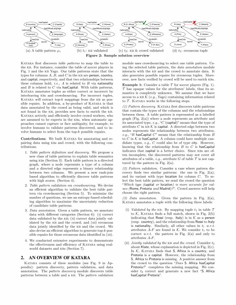
(a) A table pattern ϕs

A (Rossi)

B (Italy) C (Rome)

D (Verona)

E (Italian)

hasCapital

locatedIn

nationality

bornIn

hasOfficalLanguage

F (Proto)

hasClub

(b) t1: kb validated

A (Klate)

B (S. Africa) C (Pretoria)

D (Pirates)

E (Afrikaans)

hasCapital

locatedIn

nationality

bornIn

hasOfficalLanguage

F (P. Eliz.)

hasClub

(c) t2: kb & crowd validated

A (Pirlo)

B (Italy) C (Madrid)

D (Juve)

E (Italian)

hasCapital

locatedIn

nationality

bornIn

hasOfficalLanguage

F (Flero)

hasClub

(d) t3: erroneous tuple

Figure 2: Sample solution overview

Katara first discovers table patterns to map the table tothe kb. For instance, consider the table of soccer players inFig. 1 and the kb Yago. Our table patterns state that thetypes for columns A, B, and C in the kb are person, country,and capital, respectively, and that two relationships betweenthese columns hold, i.e., A is related to B via nationalityand B is related to C via hasCapital. With table patterns,Katara annotates tuples as either correct or incorrect byinterleaving kbs and crowdsourcing. For incorrect tuples,Katara will extract top-k mappings from the kb as pos-sible repairs. In addition, a by-product of Katara is thatdata annotated by the crowd as being valid, and which isnot found in the kb, provides new facts to enrich the kb.Katara actively and efficiently involve crowd workers, whoare assumed to be experts in the kbs, when automatic ap-proaches cannot capture or face ambiguity, for example, toinvolve humans to validate patterns discovered, and to in-volve humans to select from the top-k possible repairs.

Contributions. We built Katara for annotating and re-pairing data using kbs and crowd, with the following con-tributions.

1. Table pattern definition and discovery. We propose anew class of table patterns to explain table semanticsusing kbs (Section 3). Each table pattern is a directedgraph, where a node represents a type of a columnand a directed edge represents a binary relationshipbetween two columns. We present a new rank-joinbased algorithm to efficiently discover table patternswith high scores. (Section 4).

2. Table pattern validation via crowdsourcing. We devisean efficient algorithm to validate the best table pat-tern via crowdsourcing (Section 5). To minimize thenumber of questions, we use an entropy-based schedul-ing algorithm to maximize the uncertainty reductionof candidate table patterns.

3. Data annotation. Given a table pattern, we annotatedata with different categories (Section 6): (i) correctdata validated by the kb; (ii) correct data jointly val-idated by the kb and the crowd; and (iii) erroneousdata jointly identified by the kb and the crowd. Wealso devise an efficient algorithm to generate top-k pos-sible repairs for those erroneous data identified in (iii).

4. We conducted extensive experiments to demonstratethe effectiveness and efficiency of Katara using real-world datasets and kbs (Section 7).

2. AN OVERVIEW OF KATARAKatara consists of three modules (see Fig. 9 in Ap-

pendix): pattern discovery, pattern validation, and dataannotation. The pattern discovery module discovers tablepatterns between a table and a kb. The pattern validation

module uses crowdsourcing to select one table pattern. Us-ing the selected table pattern, the data annotation moduleinteracts with the kb and the crowd to annotate data. Italso generates possible repairs for erroneous tuples. More-over, new facts verified by crowd will be used to enrich kbs.

Example 1: Consider a table T for soccer players (Fig. 1).T has opaque values for the attributes’ labels, thus its se-mantics is completely unknown. We assume that we haveaccess to a kb K (e.g., Yago) containing information relatedto T . Katara works in the following steps.

(1) Pattern discovery. Katara first discovers table patternsthat contain the types of the columns and the relationshipsbetween them. A table pattern is represented as a labelledgraph (Fig. 2(a)) where a node represents an attribute andits associated type, e.g., “C (capital)” means that the type ofattribute C in kb K is capital. A directed edge between twonodes represents the relationship between two attributes,e.g., “B hasCapital C” means that the relationship from Bto C in K is hasCapital. A column could have multiple can-didate types, e.g., C could also be of type city. However,knowing that the relationship from B to C is hasCapitalindicates that capital is a better choice. Since kbs are of-ten incomplete, the discovered patterns may not cover allattributes of a table, e.g., attribute G of table T is not cap-tured by the pattern in Fig. 2(a).

(2) Pattern validation. Consider a case where pattern dis-covery finds two similar patterns: the one in Fig. 2(a),and its variant with type location for column C. To se-lect the best table pattern, we send the crowd the question“Which type (capital or location) is more accurate for val-ues (Rome,Pretoria and Madrid)?”. Crowd answers will helpchoose the right pattern.

(3) Data annotation. Given the pattern in Fig. 2(a),Katara annotates a tuple with the following three labels:

(i) Validated by the kb. By mapping tuple t1 in table Tto K, Katara finds a full match, shown in Fig. 2(b)indicating that Rossi (resp. Italy) is in K as a person(resp. country), and the relationship from Rossi to Italyis nationality. Similarly, all other values in t1 w.r.t.attributes A-F are found in K. We consider t1 to becorrect w.r.t. the pattern in Fig. 2(a) and only toattributes A-F .

(ii) Jointly validated by the kb and the crowd. Consider t2about Klate, whose explanation is depicted in Fig. 2(c).In K, Katara finds that S. Africa is a country, andPretoria is a capital. However, the relationship fromS. Africa to Pretoria is missing. A positive answer fromthe crowd to the question “Does S. Africa hasCapitalPretoria?” completes the missing mapping. We con-sider t2 correct and generate a new fact “S. AfricahasCapital Pretoria”.

(iii) Erroneous tuple. For tuple t3, there is also no link fromItaly to Madrid in K (Fig. 2(d)). A negative answerfrom the crowd to the question “Does Italy hasCapitalMadrid?” confirms that there is an error in t3, At thispoint, however, we cannot decide which value in t3is wrong, Italy or Madrid. Katara will then extractrelated evidences from K, such as Italy hasCapital Romeand Spain hasCapital Madrid, and use these evidencesto generate a set of possible repairs for this tuple. 2

The pattern discovery module can be used to select themore relevant kb for a given dataset. If the module cannotfind patterns for a table and a kb, Katara will terminate.

3. PRELIMINARIES

3.1 Knowledge BasesWe consider knowledge bases (kbs) as RDF-based data

consisting of resources, whose schema is defined using theResource Description Framework Schema (RDFS). A re-source is a unique identifier for a real-word entity. Forinstance, Rossi, the soccer player, and Rossi, the motorcy-cle racer, are two different resources. Resources are rep-resented using URIs (Uniform Resource Identifiers) in Yagoand DBPedia, and mids (machine-generated ids) in Freebase.A literal is a string, date, or number, e.g., 1.78. A prop-erty (a.k.a. relationship) is a binary predicate that repre-sents a relationship between two resources or between a re-source and a literal. We denote the property between re-source x and resource (or literal) y by P (x, y). For instance,locatedIn(Milan, Italy) indicates that Milan is in Italy.

An RDFS ontology distinguishes between classes and in-stances. A class is a resource that represents a set of objects,e.g., the class of countries. A resource that is a member of aclass is called an instance of that class. The type relationshipassociates an instance to a class e.g., type(Italy) = country.

A more specific class c can be specified as a subclass of amore general class d by using the statement subclassOf(c, d).This means that all instances of c are also instances of d,e.g., subclassOf(capital, location). Similarly, a property P1

can be a sub-property of a property P2 by the statementsubpropertyOf(P1, P2). Moreover, we assume that the prop-erty between an entity and its readable name is labeled with“label”, according to the RDFS schema.

Note that an RDF ontology naturally covers the case of akb without a class hierarchy such as IMDB. Also, a more ex-pressive languages, such as OWL (Web Ontology Language),can offer more reasoning opportunities at a higher computa-tional cost. However, kbs in industry [14] as well as popularones, such as Yago, Freebase, and DBpedia, use RDFS.

3.2 Table PatternsConsider a table T with attributes denoted by Ai. There

are two basic semantic annotations on a relational table.

(1) Type of an attribute Ai. The type of an attribute is anannotation that represents the class of attribute values in Ai.For example, the type of attribute B in Fig. 1 is country.

(2) Relationship from attribute Ai to attribute Aj . Therelationship between two attributes is an annotation that rep-resents how Ai and Aj are related through a directed binaryrelationship. Ai is called the subject of the relationship, andAj is called the object of the relationship. For example, therelationship from attribute B to C in Fig. 1 is hasCapital.

Table pattern. A table pattern (pattern for short) ϕ of atable T is a labelled directed graph G(V,E) with nodes Vand edges E. Each node u ∈ V corresponds to an attributein T , possibly typed, and each edge (u, v) ∈ E from u tov has a label P , denoting the relationship between two at-tributes that u and v represent. For a pattern ϕ, we denoteby ϕu a node u in ϕ, ϕ(u,v) an edge in ϕ, ϕV all nodes in ϕ,and ϕE all edges in ϕ.

We assume that a table pattern is a connected graph.When there exist multiple disconnected patterns, i.e., twotable patterns that do not share any common node, we treatthem independently. Hence, in the following, we focus ondiscussing the case of a single table pattern.

Semantics. A tuple t of T matches a table pattern ϕ con-taining m nodes {v1, . . . , vm} w.r.t. a kb K, denoted byt |= ϕ, if there exist m distinct attributes {A1, . . . , Am} inT and m resources {x1, . . . , xm} in K such that:

1. there is a one-to-one mapping from Ai (and xi) to vifor i ∈ [1,m];

2. t[Ai] ≈ xi and either type(xi) = type(vi) orsubclassOf(type(xi), type(vi));

3. for each edge (vi, vj) in ϕE with property P , thereexists a property P ′ for the corresponding resources xi

and xj in K such that P ′ = P or subpropertyOf(P ′, P ).

Intuitively, if t matches ϕ, each corresponding attributevalue of t maps to a resource r in K under a domain-specificsimilarity function (≈), and r is a (sub-)type of the typegiven in ϕ (conditions 1 and 2). Moreover, for each propertyP in a pattern, the property between the two correspondingresources must be P or its sub-properties (condition 3).

Example 2: Consider tuple t1 in Fig. 1 and pattern ϕs inFig. 2(a). Tuple t1 matches ϕs, as in Fig. 2(b), since for eachattribute value (e.g., t1[A] = Rossi and t1[B] = Italy) there isa resource in K that has a similar value with correspondingtype (person for Rossi and country for Italy) for conditions 1and 2, and the property nationality holds from Rossi to Italyin K (condition 3). Similarly, conditions 1–3 hold for otherattribute values in t1. Hence, t1 |= ϕs. 2

We say that a tuple t of T partially matches a table patternϕ w.r.t. K, if at least one of condition 2 and condition 3holds.

Example 3: Consider t2 in Fig. 1 and ϕs in Fig. 2(a).We say that t2 partially matches ϕs, since the propertyhasCapital from t2[B] = S. Africa to t2[C] = Pretoria doesnot exist in K, i.e., condition 3 does not hold. 2

Given a table T , a kb K, and a pattern ϕ, Fig. 3 showshow Katara works on T .

(1) Attributes covered by K. Attributes A–F in Fig. 1 arecovered by the pattern in Fig. 2(a). We consider two casesfor the tuples.

(a) Fully covered by K. We annotate such tuples as se-mantically correct relative to ϕ and K (Fig. 2(b)).

(b) Partially covered by K. We use crowdsourcing to ver-ify whether the non-covered data is caused by theincompleteness of K (Fig. 2(c)) or by actual errors(Fig. 2(d)).

(2) Attributes not covered by K. Attribute G in Fig. 1 is not

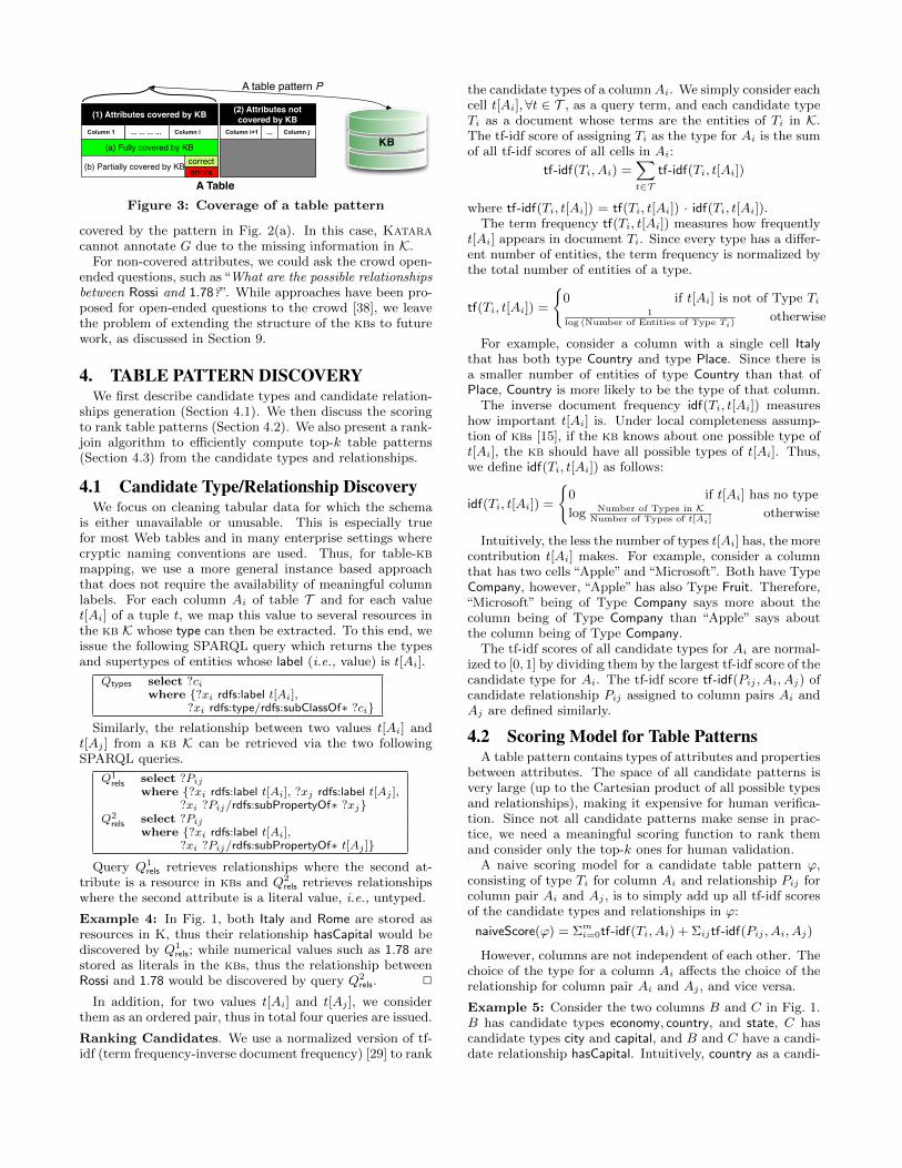
KB

(2) Attributes not covered by KB(1) Attributes covered by KB

(a) Fully covered by KB

(b) Partially covered by KB correcterrors

A table pattern P

A Table

Column 1 ... ... ... ... Column i Column i+1 ... Column j

Figure 3: Coverage of a table pattern

covered by the pattern in Fig. 2(a). In this case, Kataracannot annotate G due to the missing information in K.

For non-covered attributes, we could ask the crowd open-ended questions, such as“What are the possible relationshipsbetween Rossi and 1.78?”. While approaches have been pro-posed for open-ended questions to the crowd [38], we leavethe problem of extending the structure of the kbs to futurework, as discussed in Section 9.

4. TABLE PATTERN DISCOVERYWe first describe candidate types and candidate relation-

ships generation (Section 4.1). We then discuss the scoringto rank table patterns (Section 4.2). We also present a rank-join algorithm to efficiently compute top-k table patterns(Section 4.3) from the candidate types and relationships.

4.1 Candidate Type/Relationship DiscoveryWe focus on cleaning tabular data for which the schema

is either unavailable or unusable. This is especially truefor most Web tables and in many enterprise settings wherecryptic naming conventions are used. Thus, for table-kbmapping, we use a more general instance based approachthat does not require the availability of meaningful columnlabels. For each column Ai of table T and for each valuet[Ai] of a tuple t, we map this value to several resources inthe kb K whose type can then be extracted. To this end, weissue the following SPARQL query which returns the typesand supertypes of entities whose label (i.e., value) is t[Ai].

Qtypes select ?ciwhere {?xi rdfs:label t[Ai],

?xi rdfs:type/rdfs:subClassOf∗ ?ci}

Similarly, the relationship between two values t[Ai] andt[Aj ] from a kb K can be retrieved via the two followingSPARQL queries.

Q1rels select ?Pij

where {?xi rdfs:label t[Ai], ?xj rdfs:label t[Aj ],?xi ?Pij/rdfs:subPropertyOf∗ ?xj}

Q2rels select ?Pij

where {?xi rdfs:label t[Ai],?xi ?Pij/rdfs:subPropertyOf∗ t[Aj ]}

Query Q1rels retrieves relationships where the second at-

tribute is a resource in kbs and Q2rels retrieves relationships

where the second attribute is a literal value, i.e., untyped.

Example 4: In Fig. 1, both Italy and Rome are stored asresources in K, thus their relationship hasCapital would bediscovered by Q1

rels; while numerical values such as 1.78 arestored as literals in the kbs, thus the relationship betweenRossi and 1.78 would be discovered by query Q2

rels. 2

In addition, for two values t[Ai] and t[Aj ], we considerthem as an ordered pair, thus in total four queries are issued.

Ranking Candidates. We use a normalized version of tf-idf (term frequency-inverse document frequency) [29] to rank

the candidate types of a column Ai. We simply consider eachcell t[Ai],∀t ∈ T , as a query term, and each candidate typeTi as a document whose terms are the entities of Ti in K.The tf-idf score of assigning Ti as the type for Ai is the sumof all tf-idf scores of all cells in Ai:

tf-idf(Ti, Ai) =∑t∈T

tf-idf(Ti, t[Ai])

where tf-idf(Ti, t[Ai]) = tf(Ti, t[Ai]) · idf(Ti, t[Ai]).The term frequency tf(Ti, t[Ai]) measures how frequently

t[Ai] appears in document Ti. Since every type has a differ-ent number of entities, the term frequency is normalized bythe total number of entities of a type.

tf(Ti, t[Ai]) =

{0 if t[Ai] is not of Type Ti

1log (Number of Entities of Type Ti)

otherwise

For example, consider a column with a single cell Italythat has both type Country and type Place. Since there isa smaller number of entities of type Country than that ofPlace, Country is more likely to be the type of that column.

The inverse document frequency idf(Ti, t[Ai]) measureshow important t[Ai] is. Under local completeness assump-tion of kbs [15], if the kb knows about one possible type oft[Ai], the kb should have all possible types of t[Ai]. Thus,we define idf(Ti, t[Ai]) as follows:

idf(Ti, t[Ai]) =

{0 if t[Ai] has no type

log Number of Types in KNumber of Types of t[Ai]

otherwise

Intuitively, the less the number of types t[Ai] has, the morecontribution t[Ai] makes. For example, consider a columnthat has two cells “Apple” and “Microsoft”. Both have TypeCompany, however, “Apple” has also Type Fruit. Therefore,“Microsoft” being of Type Company says more about thecolumn being of Type Company than “Apple” says aboutthe column being of Type Company.

The tf-idf scores of all candidate types for Ai are normal-ized to [0, 1] by dividing them by the largest tf-idf score of thecandidate type for Ai. The tf-idf score tf-idf(Pij , Ai, Aj) ofcandidate relationship Pij assigned to column pairs Ai andAj are defined similarly.

4.2 Scoring Model for Table PatternsA table pattern contains types of attributes and properties

between attributes. The space of all candidate patterns isvery large (up to the Cartesian product of all possible typesand relationships), making it expensive for human verifica-tion. Since not all candidate patterns make sense in prac-tice, we need a meaningful scoring function to rank themand consider only the top-k ones for human validation.

A naive scoring model for a candidate table pattern ϕ,consisting of type Ti for column Ai and relationship Pij forcolumn pair Ai and Aj , is to simply add up all tf-idf scoresof the candidate types and relationships in ϕ:

naiveScore(ϕ) = Σmi=0tf-idf(Ti, Ai) + Σijtf-idf(Pij , Ai, Aj)

However, columns are not independent of each other. Thechoice of the type for a column Ai affects the choice of therelationship for column pair Ai and Aj , and vice versa.

Example 5: Consider the two columns B and C in Fig. 1.B has candidate types economy, country, and state, C hascandidate types city and capital, and B and C have a candi-date relationship hasCapital. Intuitively, country as a candi-

Algorithm 1 PDiscovery

Input: a table T , a KB K, and a number k.Output: top-k table patterns based on their scores1: types(Ai)← get a ranked list of candidate types for Ai

2: properties(Ai, Aj) ← get a ranked list of candidate relation-ships for Ai and Aj

3: Let P be the top-k table patterns, initialized empty4: for all Ti ∈ types(Ai), and Pij ∈ properties(Ai, Aj) in de-

scending order of tf-idf scores do5: if |P| > k and TypePruning(Ti) then6: continue7: generate all table patterns P ′ involving Ti or Pij

8: compute the score for each table pattern P in P ′9: update P using P ′

10: compute the upper bound score B of all unseen patterns,and let ϕk ∈ P be the table pattern with lowest score

11: halt when score(ϕk) > B12: return P

date type for column B is more compatible with hasCapitalthan economy since capitals are associated with countries,not economies. In addition, capital is also more compatiblewith hasCapital than city since not all cities are capitals. 2

Based on the above observation, to quantify the“compati-bility” between a type T and relationship P , where T servesas the type for the resources appearing as subjects of therelationship P , we introduce a coherence score subSC(T, P ).Similarly, to quantify the “compatibility” between a typeT and relationship P , where T serves as the type for theentities appearing as objects of the relationship P , we in-troduce a coherence scores objSC(T, P ). subSC(T, P ) (resp.objSC(T, P )) measures how likely an entity of Type T ap-pears as a subject (resp. object) of the relationship P .

We use pointwise mutual information (PMI) [10] as aproxy for computing subSC(T, P ) and objSC(T, P ). We usethe following notations: ENT(T ) - the set of entities in Kof type T , subENT(P ) - the set of entities in K that ap-pear in the subject of P , objENT(P ) - the set of entitiesin K that appear in the object of P , and N - the totalnumber of entities in K. We then consider the following

probabilities: Pr(T ) = |ENT(T )|N , the probability of an entity

belonging to T , Prsub(P ) = |subENT(P )|N , the probability of an

entity appearing in the subject of P , Probj(P ) = |objENT(P )|N ,

the probability of an entity appearing in the object of P ,

Prsub(P ∩ T ) = |ENT(T )∩subENT(P )|N , the probability of an en-

tity belonging to type T and appearing in the subject of P ,

and Probj(P ∩ T ) = |ENT(T )∩objENT(P )|N , the probability of an

entity belonging to type T and appearing in the object ofP . Finally, we can define PMIsub(T, P ):

PMIsub(T, P ) = logPrsub(P ∩ T )

Prsub(P )Pr(T )

The PMI can be normalized into [−1, 1] as follows [3]:

NPMIsub(T, P ) =PMIsub(T, P )

−Prsub(P ∩ T )

To ensure that the coherence score is in [0, 1], we definethe subject semantic coherence of T for P as

subSC(T, P ) =NPMIsub(T, P ) + 1

2The object semantic coherence of T for P can be defined

similarly.

Example 6: Below are sample coherence scores computedfrom Yago.

Algorithm 2 TypePruning

Input: current top-k table patterns P, candidate type Ti.Output: a boolean value, true/false means Ti can/cannot be

pruned1: curMinCohSum(Ai) ← minimum sum of all coherence scores

involving column Ai in current top-k P2: maxCohSum(Ai, Ti)← maximum sum of all coherence scores

if the type of column Ai is Ti

3: if maxCohSum(Ai, Ti) < curMinCohSum(Ai) then4: return true5: else6: return false

subSC(economy, hasCapital) = 0.84subSC(country, hasCapital) = 0.86objSC(city, hasCapital) = 0.69objSC(capital, hasCapital) = 0.83

These scores reflect our intuition in Example 5: country ismore suitable than economy to act as a type for the subjectresources of hasCapital; and capital is more suitable than cityto act as a type for the object resources of hasCapital. 2

We now define the score of a pattern ϕ as follows:

score(ϕ) = Σmi=0tf-idf(Ti, Ai) + Σijtf-idf(Pij , Ai, Aj)

+Σij(subSC(Ti, Pij) + objSC(Tj , Pij))

4.3 Top-k Table Pattern GenerationGiven the scoring model of table patterns, we describe how

to retrieve the top-k table patterns with the highest scoreswithout having to enumerate all candidates. We formulatethis as a rank-join problem [22]: given a set of sorted listsand join conditions of those lists, the rank-join algorithmproduces the top-k join results based on some score functionfor early termination without consuming all the inputs.

Algorithm. The algorithm, referred as PDiscovery, isgiven in Algorithm 1. Given a table T , a kb K, and anumber k, it produces top-k table patterns. To start, eachinput list, i.e., candidate types for a column, and candi-date relationships for a column pair, is ordered accordingto the respective tf-idf scores (lines 1-2). When two candi-date types (resp. relationships) have the same tf-idf scores,the more discriminative type (resp. relationship) is rankedhigher, i.e., the one with less number of instances in K.

Two lists are joined if they agree on one column, e.g.,the list of candidate types for Ai is joined with the list ofcandidate relationships for Ai and Aj . A join result is a can-didate pattern ϕ, and the scoring function is score(ϕ). Therank-join algorithm scans the ranked input lists in descend-ing order of their tf-idf scores (lines 3-4), table patterns aregenerated incrementally as we move down the input lists.Table patterns that cannot be used to produce top-k pat-terns will be pruned (lines 5-6). For each join result, i.e.,each table pattern ϕ, the score score(ϕ) is computed (lines 7-8). We also maintain an upper bound B of the scores of allunseen join results, i.e., table patterns (line 10). Since eachlist is ranked, B can be computed by adding up the sup-port scores of the current positions in the ranked lists, plusthe maximum coherence scores a candidate relationship canhave with any types. We terminate the join process if eitherwe have exhaustively scanned every input list, or we haveobtained top-k table patterns and the score of the kth tablepattern is greater than or equal to B (line 11).

Lines 5-6 in Algorithm 1 check whether a candidate typeTi for column Ai can be pruned without generating ta-

ble patterns involving Ti by calling Algorithm 2. The in-tuition behind type pruning (Algorithm 2) is that a can-didate type Ti is useful if it is more coherent with anyrelationship Pix than previously examined types for Ai.We first calculate the current minimum sum of coherencescores involving column Ai in the current top-k patterns,i.e., curMinCohSum(Ai) (line 1). We then calculate themaximum possible sum of coherence scores involving typeTi, i.e., maxCohSum(Ai, Ti) (line 2). Ti can be pruned ifmaxCohSum(Ai, Ti) < curMinCohSum(Ai) since any tablepattern having Ti as the type for Ai will have a lower scorethan the scores of the current top-k patterns (lines 3-6).

Example 7: Consider the rank-join graph in Fig. 4(k = 2) for a table with just two columns B andC as in Fig. 1. The tf-idf scores for each candi-date type and relationship are shown in the parenthe-ses. The top-2 table patterns ϕ1, ϕ2 are shown on thetop. score(ϕ1) = sup(country, B) + sup(capital, C) +sup(hasCapital, B,C) + 5 × (subSC(country, hasCapital) +objSC(capital, hasCapital)) = 1.0 + 0.9 + 0.9 + 0.86 + 0.83 =4.49. Similarly, we have score(ϕ2) = 4.47.

Suppose we are currently examining type state for columnB. We do not need to generate table patterns involving statesince the maximum coherence between state and hasCapitalor isLocatedIn is less than the the current minimum coher-ence score between type of column B and relationship be-tween B and C in the current top-2 patterns.

Suppose we are examining type whole for column C, andwe have reached type state for B and hasCapital for rela-tionship B,C. The bound score for all unseen patterns isB = 0.7 + 0.5 + 0.9 + 0.86 + 0.83 = 3.78, where 0.7, 0.9 and0.5 are the tf-idf scores for state, whole and hasCapital re-spectively, and 0.86 (resp. 0.83) is the maximum coherencescore between any type in types(B) (resp. types(C)) andany relationship in properties(B,C). Since B is smaller thanscore(ϕ2) = 4.47, we terminate the rank join process. 2

Correctness. Algorithm 1 is guaranteed to produce thetop-k table patterns since we keep the current top-k patternsin P, and we terminate when we are sure that it will notproduce any new table pattern with a higher score. In theworst case, we still have to exhaustively go through all theranked lists to produce the top-k table patterns. However,in most cases the top ranked table patterns involve onlycandidate types/relationships with high tf-idf scores, whichare at the top of the lists.

Computing coherence scores for a type and a relation-ship is an expensive operation that requires set intersection.Therefore, for a given K, we compute offline the coherencescore for every type and every relationship. For each rela-tionship, we also keep the maximum coherence score it canachieve with any type, to efficiently compute the bound B.

5. PATTERN VALIDATION VIA CROWDWe now study how to use the crowd to validate the discov-

ered table patterns. Specifically, given a set P of candidatepatterns, a table T , a kb K, and a crowdsourcing frame-work, we need to identify the most appropriate pattern forT w.r.t. K, with the objective of minimizing the number ofcrowdsourcing questions. We assume that the crowd work-ers are experts in the semantics of the reference kbs, i.e.,they can verify if values in the tables fit into the kbs.

economy(1.0)country(1.0)location(1.0)

state(0.7)…

type (B)locatedIn(1.0)

hasCapital(0.9)

relationship (B, C)City(1.0)

Capital(0.9)whole(0.5)artifact(0.1)Person(0.1)

…

type (C)

1: B (country), C (capital), hasCapital (B, C)2: B (economy), C (city), hasCapital (B, C)

''

Figure 4: Encoding top-k as a rank-join

5.1 Creating Questions for the CrowdA naive approach to generate crowdsourcing questions is

to express each candidate table pattern as a whole in a singlequestion to the crowd who would then select the best one.However, table pattern graphs can be hard for crowd users tounderstand (e.g., Fig. 2(a)). Also, crowd workers are knownto be good at answering simple questions [41]. A practicalsolution is to decompose table patterns into simple tasks:(1) type validation, i.e., to validate the type of a columnin the table pattern; and (2) binary relationship validation,i.e., to validate the relationship between two columns.

Column type validation. Given a set of candidate typescandT(Ai) for column Ai, one type Ti ∈ candT(Ai) needsto be selected. We formulate the following question to thecrowd about the type of a column: What is the most accuratetype of the highlighted column?; along with kt randomly cho-sen tuples from T and all candidate types from candT(Ai).A sample question is given as follows.

Q1 :What is the most accurate type of the highlighted column?

(A, B , C, D, E, F , ...)

(Rossi, Italy , Rome, Verona, Italian, Proto, ...)

(Pirlo, Italy , Madrid, Juve, Italian, Flero”

...)

© country © economy© state © none of the above

After q questions are answered by the crowd workers, thetype with the highest support from the workers is chosen.

Crowd workers, even if experts in the reference kb, areprone to mistakes when t[Ai] in tuple t is ambiguous, i.e.,t[Ai] belongs to multiple types in candT(Ai). However, thisis mitigated by two observations: (i) it is unlikely that allvalues are ambiguous and (ii) the probability of providingonly ambiguous values diminishes quickly with respect tothe number of values. Consider two types T1 and T2 incandT(Ai), the probability that randomly selected entities

belong to both types is p = |ENT (T1)∩ENT (T2)||ENT (T1)∪ENT (T2)| . After q

questions are answered, the probability that all q · kt valuesare ambiguous is pq·kt . Suppose p = 0.8, a very high for twotypes in K, and five questions are asked with each questioncontaining five tuples, i.e., q = 5, kt = 5, the probabilitypq·kt becomes as low as 0.0038.

For each question, we also expose some contextual at-tribute values that help workers better understand the ques-tion. For example, we expose the values for A,C,D,E inquestion Q1 when validating the type of B. If the the num-ber of attributes is small, we show them all; otherwise, weuse off-the-shelf technology to identify attributes that arerelated to the ones in the question [23]. To mitigate the riskof workers making mistakes, each question is asked threetimes, and the majority answer is taken. Indeed, our empir-

ical study in Section 7.2 shows that five questions are enoughto pick the correct type in all the datasets we experimented.

Relationship validation. We validate the relationship forcolumn pairs in a similar fashion, with an example below.

Q2 :What is the most accurate relationship for

highlighted columns (A, B, C , D, E, F , ...)

(Rossi, Italy, Rome , Verona, Italian, Proto, ...)

(Pirlo, Italy, Madrid , Juve, Italian, Flero, ...)

© B hasCapital C © C locatedIn B © none of the above

Candidate types and candidate relationships are storedas URIs in kbs; thus not directly consumable by thecrowd workers. For example, the type capital is stored ashttp://yago-knowledge.org/resource/wordnet capital 10851850,and the relationship hasCapital is stored as http://yago-

knowledge.org/resource/hasCapital. We look up type andrelationship descriptions, e.g., capital and hasCapital, byquerying the kb for the labels of the corresponding URIs.If no label exists, we process the URI itself by removing thetext before the last slash and punctuation symbols.

5.2 Question SchedulingWe now turn our attention to how to minimize the total

number of questions to obtain the correct table pattern byscheduling which column and relationship to validate first.

Note that once a type (resp. relationship) is validated, wecan prune from P all table patterns that have a different type(resp. relationship) for that column (resp. column pair).Therefore, a natural choice is to choose those columns (resp.column pairs) with the maximum uncertainty reduction [45].

Consider ϕ as a variable, which takes values from P ={ϕ1, ϕ2, . . . , ϕk}. We translate the score associated witheach table pattern to a probability by normalizing the

scores, i.e., Pr(ϕ = ϕi) = score(ϕi)Σϕj∈Pscore(ϕj)

. Our transla-

tion from scores to probabilities follows the general frame-work of interpreting scores in [25]. Specifically, our trans-lation is rank-stable, i.e., for two patterns ϕ1 and ϕ2, ifscore(ϕ1) > score(ϕ2), then Pr(ϕ = ϕ1) > Pr(ϕ = ϕ2).

We define the uncertainty of ϕ w.r.t. P as the entropy.

HP(ϕ) = −Σϕi∈PPr(ϕ = ϕi) log2 Pr(ϕ = ϕi)

Example 8: Consider an input list of five table patternsP = {ϕ1, . . . , ϕ5} as follows with the normalized probabilityof each table pattern shown in the last column.

type (B) type (C) P (B,C) score probϕ1 country capital hasCapital 2.8 0.35ϕ2 economy capital hasCapital 2 0.25ϕ3 country city locatedIn 2 0.25ϕ4 country capital locatedIn 0.8 0.1ϕ5 state capital hasCapital 0.4 0.05

2

We use variables vAi and vAiAj to denote the type of thecolumn Ai and the relationship between Ai and Aj respec-tively. The set of all variables is denoted as V . In Exam-ple 8, V = {vB , vC , vBC}, vB ∈ {country, economy, state},vC ∈ {capital, city} and vBC ∈ {hasCapital, isLocatedIn}.The probability of an assignment of a variable v to a is ob-tained by aggregating the probability of those table patternsthat have that assignment for v. For example, Pr(vB =country) = Pr(ϕ1) +Pr(ϕ3) +Pr(ϕ4) = 0.35 + 0.25 + 0.1 =0.7, Pr(vB = economy) = 0.25, and Pr(vB = state) = 0.05.

Algorithm 3 PatternValidation

Input: a set of table patterns POutput: one table pattern ϕ ∈ P1: Pre be the remaining table patterns, initialized P2: initialize all variables V , representing column or column pairs,

and calculate their probability distributions.3: while |Pre| > 1 do4: Ebest ← 05: vbest ← null6: for all v ∈ V do7: compute the entropy H(v).8: if H(v) > Ebest then9: vbest ← v

10: Ebest ← H(v)11: validate the variable v, suppose the result is a, let Pv=a

to be the set of table patterns with v = a12: Pre = Pv=a

13: normalize the probability distribution of patterns in Pre.14: return the only table pattern ϕ in Pre

After validating a variable v to have value a, we removefrom P those patterns that have different assignment forv. The remaining patterns are denoted as Pv=a. Sup-pose column B is validated to be of type country, thenPvB=country = {ϕ1, ϕ3, ϕ4}. Since we do not know what valuea variable can take, we measure the expected reduction ofuncertainty of variable ϕ after validating variable v, formallydefined as:

E(∆H(ϕ))(v) = ΣaPr(v = a)HPv=a(ϕ)−HP(ϕ)

In each iteration, we choose the variable v (columnor column pair) with the maximum uncertainty reduc-tion, i.e., E(∆H(ϕ))(v). Each iteration has a complex-ity of O(|V ||P|2) because we need to examine all |V | vari-ables, each variable could take |P| values, and calculatingHPv=a(ϕ) for each value also takes O(|P|) time. The follow-ing theorem simplifies the calculation for E(∆H(v)) with acomplexity of O(|V ||P|).

Theorem 1. The expected uncertainty reduction aftervalidating a column (column pair) v is the same as theentropy of the variable. E(∆H(ϕ))(v) = H(v), whereH(v) = −ΣaPr(v = a) log2 Pr(v = a).

The proof of Theorem 1 can be found in Appendix A.Algorithm 3 describes the overall procedure for pattern val-idation. At each iteration: (1) we choose the best variablevbest to validate next based on the expected reduction ofuncertainty of ϕ (lines 4-10); (2) we remove from Pre thosetable patterns that have a different assignment for variablev than the validated value a (lines 11-12); and (3) we renor-malize the probability distribution of the remaining tablepatterns in Pre (line 13). We terminate when we are leftwith only one table pattern (line 3).

Example 9: To validate the five patterns in Example 8,we first calculate the entropy of every variable. H(vB) =−0.7 log2 0.7− 0.25log20.25− 0.05log20.05 = 1.07, H(vC) =0.81, and H(vBC) = 0.93. Thus column B is validated first,say the answer is country. The remaining set of table pat-terns, and their normalized probabilities are:

type (B) type (C) P (B,C) probϕ1 country capital hasCapital 0.5ϕ3 country city locatedIn 0.35ϕ4 country capital locatedIn 0.15

Now Pre = {ϕ1, ϕ3, ϕ4}. The new entropies are: H(vB) =0, H(vC) = 0.93 and H(vBC) = 1. Therefore, column pair

A (Pirlo)

B (Italy) C (Rome)

D (Juve)

E (Italian)

hasCapital

locatedIn

nationality

bornIn

hasOfficalLanguage

F (Flero)

hasClub

(a) Possible repair G1

A (Xabi Alonso)

B (Spain) C (Madrid)

D (Real Madrid)

E (Spanish)

hasCapital

locatedIn

nationality

bornIn

hasOfficalLanguage

F (Tolosa)

hasClub

(b) Possible repair G2

Figure 5: Sample instance graphs

B,C is chosen, say the answer is hasCapital. We are now leftwith only one pattern ϕ1, thus we return it. 2

In Example 9, we do not need to validate vC following ourscheduling strategy. Furthermore, after validating certainvariables, other variables may become less uncertain, thusrequiring a smaller number of questions to validate.

6. DATA ANNOTATIONIn this section, we describe how Katara annotates data

(Section 6.1). We also discuss how to generate possible re-pairs for identified errors (Section 6.2).

6.1 Annotating DataKatara annotates tuples as correct data validated by kbs,

correct data jointly validated by kbs and the crowd, or dataerrors detected by the crowd, using the following two steps.

Step 1: Validation by kbs. For each tuple t and pattern ϕ,Katara issues a SPARQL query to check whether t is fullycovered by a kb K. If it is fully covered, Katara annotatesit as a correct tuple validated by kb (case (i)). Otherwise,it goes to step 2.

Step 2: Validation by kbs and Crowd. For each node (i.e.,type) and edge (i.e., relationship) that is missing from K,Katara asks the crowd whether the relationship holds be-tween the given two values. If the crowd says yes, Kataraannotates it as a correct tuple, jointly validated by kb andcrowd (case (ii)). Otherwise, it is certain that there existerrors in this tuple (case (iii)).

Example 10: Consider tuple t2 (resp. t3) in Fig. 1 and thetable pattern in Fig. 2(a). The information about whetherPretoria (resp. Madrid) is a capital of S. Africa (resp. Italy)is not in kb. To verify this information, we issue a booleanquestion Qt2 (resp. Qt3) to the crowd as:

Qt2 :Does S. Africa hasCapital Pretoria?© Yes © No

Qt3 :Does Italy hasCapital Madrid?© Yes © No

In such case, the crowd will answer yes (resp. no) toquestion Qt2 (resp. Qt3). 2

Knowledge base enrichment. Note that, in step 2, foreach affirmative answer from the crowd (e.g., Qt2 above), anew fact that is not in the current kb is created. Kataracollects such facts and uses them to enrich the kb.

6.2 Generating Top-k Possible RepairsWe start by introducing two notions that are necessary to

explain our approach for generating possible repairs.

Instance graphs. Given a kb K and a pattern G(V,E),an instance graph GI(VI , EI) is a graph with nodes VI and

Algorithm 4 Top-k repairs

Input: a tuple t, a table pattern ϕ, and inverted lists LOutput: top-k repairs for t1: Gt = ∅2: for each attribute A in ϕ do3: Gt = Gt ∪ L(A, t[A])4: for each G in Gt do5: compute cost(t, ϕ,G)6: return top-k repairs in Gt with least cost values

edges EI , such that (i) each node vi ∈ VI is a resource in K;(ii) each edge ei ∈ EI is a property in K; (iii) there is a one-to-one correspondence f from each node v ∈ V to a nodevi ∈ VI , i.e., f(v) = vi; and (iv) for each edge (u, v) ∈ E,there is an edge (f(u), f(v)) ∈ EI with the same property.Intuitively, an instance graph is an instantiation of a patternin a given kb.

Example 11: Figures 5(a) and 5(b) are two instance graphsof the table pattern of Fig. 2(a) in Yago for two players. 2

Repair cost. Given an instance graph G, a tuple t, and atable pattern ϕ, the repair cost of aligning t to G w.r.t. ϕ,

denoted by cost(t, ϕ,G) =n∑

i=1

ci, is the cost of changing

values in t to align it with G, where ci is the cost of the i-thchange and n the number of changes in t. Intuitively, the lessa repair cost is, the closer the updated tuple is to the originaltuple, hence more likely to be correct. By default, we setci = 1. The cost can also be weighted with confidences ondata values [18]. In such case, the higher the confidencevalue is, the more costly the change is.

Example 12: Consider tuple t3 in Fig. 1, the table patternϕs in Fig. 2(a), and two instance graphs G1 and G2 in Fig. 5.The repair cost to update t3 to G1 is 1, i.e., cost(t3, ϕs, G1)= 1, by updating t3[C] from Madrid to Rome. Similarly, therepair cost from t3 to G2 is 5, i.e., cost(t3, ϕs, G2) = 5. 2

Note that the possible repairs are ranked based on repaircost in ascending order. We provide top-k possible repairsand we leave it to the users (or crowd) to pick the mostappropriate repair. In the following, we describe algorithmsto generate top-k repairs for each identified erroneous tuple.

Given a kb K and a pattern ϕ, we compute all instancegraphs G in K w.r.t. ϕ. For each tuple t, a naive solution isto compute the distance between t and each graph G in G.The k graphs with smallest repair cost are returned as top-kpossible repairs. Unfortunately, this is too slow in practice.

A natural way to improve the naive solution for top-kpossible repair generation is to retrieve only instance graphsthat can possibly be repairs, i.e., the instance graphs whosevalues have an overlap with a given erroneous tuple. Weleverage inverted lists to achieve this goal.

Inverted lists. Each inverted list is a mapping from a key toa posting list. A key is a pair (A, a) where A is an attributeand a is a constant value. A posting list is a set G of graphinstances, where each G ∈ G has value a on attribute A.

For example, an inverted list w.r.t. G1 in Fig. 5(a) is as:

country, Italy → G1

Algorithm. The optimized algorithm for a tuple t is givenin Algorithm 4. All possible repairs are initialized (line 1)and instantiated by using inverted lists (lines 2-3). For each

possible repair, its repair cost w.r.t. t is computed (lines 4-5), and top-k repairs are returned (line 6).

Example 13: Consider t3 in Fig. 1 and pattern ϕs inFig. 2(a). The inverted lists retrieved are given below.

A, Pirlo → G1 X D, Juve → G1 XB, Italy → G1 X E, Italian → G1 XC, Madrid → G2 X F, Flero → G1 X

It is easy to see that the occurrences of instance graphsG1 and G2 are 5 and 1, respectively. In other words, thecost of repairing t3 w.r.t. G1 is 6 − 5 = 1 and w.r.t. G2 is6− 1 = 5. Hence, the top-1 possible repair for t3 is G1. 2

The practicability of possible repairs of Katara dependson the coverage of kbs, while existing automatic data re-pairing techniques usually require certain redundancy in thedata to perform well. Katara and existing techniques com-plement each other, as demonstrated in Section 7.4.

7. EXPERIMENTAL STUDYWe evaluated Katara using real-life data along four di-

mensions: (i) the effectiveness and efficiency of table patterndiscovery (Section 7.1); (ii) the efficiency of pattern valida-tion via the expert crowd (Section 7.2); (iii) the effectivenessand efficiency of data annotation (Section 7.3); and (iv) theeffectiveness of possible repairs (Section 7.4).

Knowledge bases. We used Yago [21] and DBpedia [27] asthe underlying kbs. Both were transformed to Jena format(jena.apache.org/) with LARQ (a combination of ARQand Lucene) support for string similarity. We set the thresh-old to 0.7 in Lucene to check whether two strings match.

Datasets. We used three datasets: WikiTables andWebTables contains tables from the Web2 with relativelysmall numbers of tuples and columns, and RelationalTablescontains tables with larger numbers of tuples and columns.• WikiTables contains 28 tables from Wikipedia pages. Theaverage number of tuples is 32.• WebTables contains 30 tables from Web pages. The aver-age number of tuples is 67.• RelationalTables has three tables: Person has personal in-formation joined on the attribute country from two sources:a biographic table extracted from wikipedia [32], and a coun-try table obtained from a wikipedia page3 resulting in 316Ktuples. Soccer has 1625 tuples about soccer players and theirclubs scraped from the Web4. University has 1357 tuplesabout US universities with their addresses5.

All the tables were manually annotated using types and re-lationships in Yago as well as DBPedia, which we consideredas the ground truth. Table 1 shows the number of columnsthat have types, and the number of column pairs that haverelationships, using Yago and DBPedia, respectively.

All experiments were conducted on Win 7 with an Intel i7CPU@3.4Ghz, 20GB of memory, and an SSD 500GB harddisk. All algorithms were implemented in JAVA.

2http://www.it.iitb.ac.in/~sunita/wwt/

3http://tinyurl.com/qhhty3p

4www.premierleague.com/en-gb.html, www.legaseriea.it/en/,

www.premierleague.com/en-gb.html5ope.ed.gov/accreditation/GetDownLoadFile.aspx

Yago DBPedia#-type #-relationship #-type #-relationship

WikiTables 54 15 57 18WebTables 71 33 73 35RelationalTables 14 7 14 16

Table 1: Datasets and kbs characteristics

7.1 Pattern DiscoveryAlgorithms. We compared four discovery algorithms.

(i) RankJoin - our proposed approach (Section 4).

(ii) Support - a baseline approach that ranks the candidatetypes and relationships solely on their support scores, i.e.,the number of tuples that are of the candidate’s types andrelationships.

(iii) MaxLike [39] - infers the type of a column and the rela-tionship between a column pair separately using maximumlikelihood estimation.

(iv) PGM [28] - infers the type of a column, the relationshipbetween column pairs, and the entities of cells by building aprobabilistic graphic model to make holistic decisions.

Evaluation Metrics. A type (relationship) gets a score of1 if it matches the ground truth, and a partial score 1

s+1

if it is the super type (relationship) of the ground truth,where s is the number of steps in the hierarchy to reach theground truth. For example, a label Film for a column, whoseactual type is IndianFilm, will get a score of 0.5, since Filmis the super type of IndianFilm with s = 1. The precision Pof a pattern ϕ is defined as the sum of scores for all typesand relationships in ϕ over the total number of types andrelationships in ϕ. The recall R of ϕ is defined as the sumof scores for all types and relationships in ϕ over the totalnumber of types and relationships in the ground truth.

Effectiveness. Table 2 shows the precision and recall ofthe top pattern chosen by four pattern discovery algorithmsfor three datasets using Yago and DBPedia. We first dis-cuss Yago. (1) Support has the lowest precision and re-call in all scenarios, since it selects the types/relationshipsthat cover the most number of tuples, which are usuallythe general types, such as Thing or Object. (2) MaxLikeuses maximum likelihood estimation to select the besttype/relationship that maximizes the probability of val-ues given the type/relationship. It performs better thanSupport, but still chooses types and relationships inde-pendently. (3) PGM is a supervised learning approachthat requires training and tuning of a number of weights.PGM shows mixed effectiveness results: it performs betterthan MaxLike on WebTables, but worse on WikiTables andRelationalTables. (4) RankJoin achieves the highest preci-sion and recall due to its tf-idf style ranking, as well as forconsidering the coherence between types and relationships.For example, consider a table with two columns actors andfilms that have a relationship actedIn. If most of the val-ues in the films column also happen to be books, MaxLikewill use books as the type, since there are fewer instances ofbooks than films in Yago. However, RankJoin would cor-rectly identify films as the type, since it is more coherentwith actedIn than books.

The result from DBPedia, also shown in Table 2, confirmsthat RankJoin performs best among the four methods. No-tice that the precision and recall of all methods are consis-tently better using DBPedia than Yago. This is because the

Support MaxLike PGM RankJoin

P R P R P R P RWikiTables .54 .59 .62 .68 .60 .67 .78 .86WebTables .65 .64 .63 .62 .77 .77 .86 .84RelationalTables .51 .51 .71 .71 .53 .53 .77 .77

Yago

P R P R P R P RWikiTables .56 .70 .71 .89 .61 .77 .71 .89WebTables .65 .69 .80 .84 .76 .80 .82 .87RelationalTables .64 .67 .81 .86 .74 .77 .81 .86

DBPedia

Table 2: Pattern discovery precision and recall

0.6

0.65

0.7

0.75

0.8

0.85

0.9

0.95

1

0 2 4 6 8 10 12 14 16 18 20

F-Measure at k

k

Support MaxLike

PGM RankJoin

(a) Yago

0.6

0.65

0.7

0.75

0.8

0.85

0.9

0.95

1

0 2 4 6 8 10 12 14 16 18 20

F-Measure at k

k

Support MaxLike

PGM RankJoin

(b) DBPedia

Figure 6: Top-k F-measure (WebTables)

number of types in DBPedia (865) is much smaller than thatof Yago (374K), hence, the number of candidate types for acolumn using DBPedia is much smaller, causing less stressfor all algorithms to rank them.

To further verify the effectiveness of our ranking function,we report the F-measure F of the top-k patterns chosen byevery algorithm. The F value of the top-k patterns is de-fined as the best value of F from one of the top-k patterns.Figure 6 shows F values of the top-k patterns varying k onWebTables. RankJoin converges faster than other methodson Yago, while all methods converge quickly on DBPedia dueto its small number of types. Top-k F-measure results for theother two datasets show similar behavior, and are reportedin Appendix B.

Efficiency. Table 3 shows the running time in secondsfor all datasets. We ran each test 5 times and reportthe average time. We separate the discussion of Personfrom RelationalTables due to its large number of tuples.For Person, we implemented a distributed version of can-didate types/relationships generation by distributing the316K tuples over 30 machines, and all candidates are col-lected into one machine to complete the pattern discovery.Support, MaxLike, and RankJoin have similar performancein all datasets, because their most expensive operation isthe disk I/Os for kbs lookups in generating candidate typesand relationships, which is linear w.r.t. the number of tu-ples. PGM is the most expensive due to the message passingalgorithms used for the inference of probabilistic graphicalmodel. PGM takes hours on tables with around 1K tuples,and cannot finish within one day for Person.

7.2 Pattern ValidationGiven the top-k patterns from the pattern discovery, we

need to identify the most appropriate one. We validatedthe patterns of all datasets using an expert crowd with 10students. Each question contains five tuples, i.e., kt = 5.

We first evaluated the effect of the number of ques-tions used to validate each variable, which is a type or arelationship, on the quality of the chosen pattern. We mea-

Support MaxLike PGM RankJoin

WikiTables 153 155 286 153WebTables 160 177 1105 162RelationalTables/Person 130 140 13842 127Person 252 258 N.A. 257

Yago

WikiTables 50 54 90 51WebTables 103 104 189 107RelationalTables/Person 400 574 11047 409Person 368 431 N.A. 410

DBPedia

Table 3: Pattern discovery efficiency (seconds)

0.92

0.93

0.94

0.95

0.96

0.97

0.98

0.99

1 2 3 4 5 6 7 8 9

P/R

q

Precision

Recall

(a) Yago

0.993

0.994

0.995

0.996

0.997

0.998

0.999

1

1 2 3 4 5 6 7 8 9

P/R

q

Precision

Recall

(b) DBPedia

Figure 7: Pattern validation P/R (WebTables)

Yago DBPediaMUVF AVI MUVF AVI

WikiTables 64 79 88 102WebTables 81 105 90 118RelationalTables 24 28 28 36

Table 4: #-variables to validate

sure the precision and recall of the final chosen validationw.r.t. the ground truth in the same way as in Section 7.1.Figure 7 shows the average precision and recall of the val-idated pattern of WebTables while varying the number ofquestions q per variable. It can be seen that, even withq = 1, the precision and recall of the validated pattern isalready high. In addition, the precision and recall convergequickly, with q = 5 on Yago, and q = 3 on DBPedia. Patternvalidation results on WikiTables and RelationalTables show asimilar behavior, and are reported in Appendix C.

To evaluate the savings in crowd pattern validation thatare achieved by our scheduling algorithm, we comparedour method (denoted MUVF, short for most-uncertain-variable-first) with a baseline algorithm (denoted AVI forall-variables-independent) that validates every variable in-dependently. For each dataset, we compared the number ofvariables needed to be validated until there is only one tablepattern left. Table 4 shows that MUVF performs consistentlybetter than AVI in terms of the number of variables to vali-date, because MUVF may spare validating certain variablesdue to scheduling, i.e., some variables become certain aftervalidating some other variables.

The validated table patterns of RelationalTables for bothYago and DBPedia are depicted in Fig. 10 in the Appendix.All validated patterns are also used in the following experi-mental study.

7.3 Data AnnotationGiven the table patterns obtained from Section 7.2, data

values are annotated w.r.t. types and relationships in thevalidated table patterns, using kbs and the crowd. Theresult of data annotation is shown in Table 5. Note that

type relationship

kb crowd error kb crowd errorWikiTables 0.60 0.39 0.01 0.56 0.42 0.02WebTables 0.69 0.28 0.03 0.56 0.39 0.05RelationalTables 0.83 0.17 0 0.89 0.11 0

Yago

kb crowd error kb crowd errorWikiTables 0.73 0.25 0.02 0.60 0.36 0.04WebTables 0.74 0.24 0.02 0.56 0.39 0.05RelationalTables 0.90 0.10 0 0.91 0.09 0

DBPedia

Table 5: Data annotation by kbs and crowd

0

0.2

0.4

0.6

0.8

1

1 2 3 4 5 6 7 8 9

F-Measure at k

k

person university

(a) Yago

0

0.2

0.4

0.6

0.8

1

1 2 3 4 5 6 7 8 9

F-Measure at k

k

person soccer

university

(b) DBPedia

Figure 8: Top-k repair F-measure (RelationalTables)

Katara annotates data in three categories (cf. Section 6.1):when kb has coverage for a value, the value is said to be vali-dated by the kb (kb column in Table 5), when the kb has nocoverage, the value is either validated by the crowd (crowdcolumn in Table 5), or the value is erroneous (error column inTable 5). Table 5 shows the breakdown of the percentage ofvalues in each category. Data values validated by the crowdcan be used to enrich the kbs. For example, a column in oneof the table in WebTables is discovered to be the type state

capitals in the United States. Surprisingly, there areonly five instances of that type in Yago6, we can add therest of 45 state capitals using values from the table to en-rich Yago. Note that the percentage of kb validated data ismuch higher for RelationalTables than it is for WikiTables andWebTables. This is because data in RelationalTables is moreredundant (e.g., Italy appears in many tuples in Person ta-ble), when a value is validated by the crowd, it will be addedto the kb, thus future occurrences of the same value will beautomatically validated by the kb.

7.4 Effectiveness of Possible RepairsIn these experiments, we evaluate the effectiveness of our

possible repairs generation by (1) varying the number k ofpossible repairs; and (2) comparing with other state of theart automatic data cleaning techniques.

Metrics. We use standard precision, recall, and F-measurefor the evaluation, which are defined as follows.

precision = (#-corrected changed values)/(#-all changes)recall = (#-corrected changed values)/(#-all errors)F-measure= 2× (precision× recall)/(precision + recall)

For comparison with automatic data cleaning approaches,we used an equivalence-class [2] (i.e., EQ) based ap-proach provided by an open-source data cleaning toolNADEEF [12], and a ML-based approach SCARE [43].When Katara provides nonempty top-k possible repairs fora tuple, we count it as correct if the ground truth falls inthe possible repairs, otherwise incorrect.

6http://tinyurl.com/q65yrba

Katara (Yago) Katara (DBPedia) EQ SCARE

P R P R P R P RPerson 1.0 0.80 1.0 0.94 1.0 0.96 0.78 0.48Soccer N.A. 0.97 0.29 0.66 0.29 0.66 0.37University 0.95 0.74 1.0 0.18 0.63 0.04 0.85 0.21

Table 6: Data repairing precision and recall(RelationalTables)

Since the average number of tuples in WikiTables andWebTables is 32 and 67, respectively, both datasets arenot suitable since both EQ and SCARE require reason-able data redundancy to compute repairs. Hence, we useRelationalTables for comparison. We learn from Table 5 thattables in RelationalTables are clean, and thus are treated asground truth. Thus, for each table in RelationalTables, weinjected 10% random errors into columns that are covered bythe patterns to obtain a corresponding dirty instance, thatis, each tuple has a 10% chance of being modified to containerrors. Moreover, in order to set up a fair comparison, weused FDs for EQ that cover the same columns as the crowdvalidated table patterns (see Appendix D). SCARE requiresthat some columns to be correct. To enable SCARE to run,we only injected errors to the right hand side attributes ofthe FDs, and treated the left hand side attributes as correctattributes (a.k.a. reliable attributes in [43]).

Effectiveness of k. We examined the effect of using top-krepairs in terms of F-measure. The results for both Yagoand DBPedia are shown in Fig. 8. The result for soccer usingYago is missing since the discovered table pattern does notcontain any relationship (cf. Fig. 10 in Appendix). Thus,Katara cannot be used to compute possible repairs w.r.t.Yago. We can see the F-measure stabilizes at k = 1 usingYago, and stabilizes at k = 3 using DBPedia. The result tellsus that in general the correct repairs fall into the top ones,which justifies our ranking of possible repairs. Next, wereport the quality of possible repairs generated by Katara,fixing k = 3.

Results of RelationalTables. The precision/recall of Katara,EQ and SCARE on RelationalTables, are reported in Table 6.The result shows that Katara always has a high precisionin cases where kbs have enough coverage of the input data.It also indicates that if Katara can provide top-k repairs,it has a good chance that the ground truth will fall in them.The recall of Katara depends on the coverage of the kbs

of the input dataset. For example, DBPedia has a lot ofinformation for Person, but relatively less for Soccer andUniversity. Yago cannot be used to repair Soccer because itdoes not have relationships for Soccer.

Both EQ and SCARE have precision that is generally lowerthan Katara, because EQ targets at computing a consistentdatabase with the minimum number of changes, which arenot necessarily the correct changes, and the result of SCAREdepends on many factors, such as the quality of the trainingdata in terms of its redundancy, and a threshold ML param-eter that is hard to set precisely. The recall for both EQ andSCARE is highly dependent on data redundancy, becausethey both require repetition of data to either detect errors.

Results of WikiTables and WebTables. Table 7 shows the re-sult of data repairing for WikiTables and WebTables. BothEQ and SCARE are not applicable on WikiTables andWebTables, because there is almost no redundancy in them.

Katara (Yago) Katara (DBPedia) EQ SCARE

P R P R P/R P/RWikiTables 1.0 0.11 1.0 0.30 N.A.WebTables 1.0 0.40 1.0 0.46 N.A.

Table 7: Data repairing precision and recall(WikiTables and WebTables)

Since there is no ground truth available for WikiTables andWebTables, we manually examine the top-3 possible repairsreturned by Katara. As we can see, Katara achieves highprecision on WikiTables and WebTables as well. In total,Katara fixed 60 errors out of 204 errors, which is 29%. Infact, most of remaining errors in these tables are null valueswhose ground truth values are not covered by given kbs.

Summary. It can be seen that Katara complements existingautomatic repairing techniques: (1) EQ and SCARE cannotbe applied to WebTables and WikiTables since there is notenough redundancy, while Katara can, given kbs and thecrowd; (2) Katara cannot be applied when there is no cov-erage in the kbs, such as the case of Soccer with Yago; and(3) when both Katara and automatic techniques can beapplied, Katara usually achieves higher precision due toits use of kbs and experts, while automatic techniques usu-ally make heuristic changes. The recall of Katara dependson the coverage of the kbs, while the recall of automatictechniques depends on the level of redundancy in the data.

8. RELATED WORKThe traditional problems of matching relational tables and

aligning ontologies have been largely studied in the databasecommunity. A matching approach where the user is alsoaware of the target schema has been recently proposed [34].Given a source and a target single relation, the user popu-lates the empty target relation with samples of the desiredoutput until a unique mapping is identified by the system. Arecent approach that looks for isomorphisms between ontolo-gies is PARIS [37], which exploits the rich information in theontologies in a holistic approach to the alignment. Unfor-tunately, our source is a relational table and our target is anon-empty labeled graph, which make these proposals hardto apply directly. On one hand, the first approach requiresto project all the entities and relationships in the target kbas binary relations, which leads to a number of target rela-tions to test that is quadratic w.r.t. the number of entities,and only few instances in the target would match with thesource data. On the other hand, the second approach re-quires to test 2n combinations of source attributes, given arelation with n attributes. The reason is that PARIS relieson structural information, thus all possible attributes shouldbe tested together to get optimal results. If we tested onlybinary relations, structural information would not be usedand inconsistent matches may arise. For example, attributesA,B can be matched with X,Y in the KB, while at the sametime, attributes B,C may match Z,W , resulting in incon-sistency (Attribute B matches two different classes X andZ). Katara actually solves this problem by first retrievingtop-k types and relationships, and then using a rank-joinbased approach to obtain the most coherent pattern.

Another line of related work is known as Web tables se-mantics understanding, which identifies the type of a columnand the relationship between two columns w.r.t. a givenkb, for the purpose of serving Web tables to search applica-

tions [13, 28, 39]. Our pattern discovery module shares thesame goal. Compared with the state of the art [28, 39], ourrank join algorithm shows superiority in both effectivenessand efficiency, as demonstrated in the experiments.

Several attempts have been made to do repairing basedon integrity constraints (ICs) [1, 9, 11, 17, 20]; they try tofind a consistent database that satisfies given ICs in a mini-mum cost. It is known that the above heuristic solutions donot ensure the accuracy of data repairing [19]. To improvethe accuracy of data repairing, experts have been involvedas first-class citizen of data cleaning systems [19, 35, 44],high quality reference data has been leveraged [19, 24, 42],and confidence values have been placed by the users [18].Katara differs from them in that Katara leverages kbs asreference data. As remarked earlier, Katara and IC basedapproaches complement each other.

Numerous studies have attempted to discover data qual-ity rules, e.g., for CFDs [6] and for DCs [8]. Automaticallydiscovered rules are error-prone, thus cannot be directly fedinto data cleaning systems without verification by domainexperts. However, and as noted earlier, they can exploit theoutput of Katara, as rules are easier to discover from cleansamples of the data [8].

Another line of work studies the problem of combiningontological reasoning with databases [5, 33]. Although theiroperation could also be used to enforce data validation, ourwork differs in that we do not assume knowledge over theconstraints defined on the ontology. Moreover, constraintsare usually expressed with FO logic fragments that restrictthe expressive power to enable polynomial complexity in thequery answering. Since we limit our queries to instance-checking over RDFS, we do not face these complexity issues.

One concern with regards to the applicability of Katarais the accuracy and coverage of the kbs and the qualityof crowdsourcing: neither the kbs nor the crowdsourcingis ensured to be completely accurate. There are several ef-forts that aim at improving the quality and coverage of bothkbs [14–16] and crowdsourcing [4, 26]. With more accurateand big kbs, Katara can discover the semantics of morelong tail tables, and further alleviate the involvement of ex-perts. A full discussion of the above topics lies beyond thescope of this work. Nevertheless, kbs and experts are usu-ally more reliable than the data at hand, thus can be treatedas relatively trusted resources to pivot on.

9. CONCLUSION AND FUTURE WORKWe proposed Katara, the first end-to-end system that

bridges knowledge bases and crowdsourcing for high qualitydata cleaning. Katara first establishes the correspondencebetween the possibly dirty database and the available kbs

by discovering and validating the table patterns. Then eachtuple in the database is verified using a table pattern againsta kb with possible crowd involvement when the kb lackscoverage. Experimental results have demonstrated both theeffectiveness and efficiency of Katara.

One important future work is to cold-start Katara whenthere is no available kbs to cover the data, i.e., bootstrap-ping and extending the kbs at the intensional level by so-liciting structural knowledge from the crowd. It would bealso interesting to assess the effects of using multiple kbs

together to repair one dataset. Another line of work is toextend our current definition of tables patterns, such as aperson column A1 is related to a country column A2 via tworelationships: A1 wasBornIn city, and city isLocatedIn A2.

10. REFERENCES[1] S. Abiteboul, R. Hull, and V. Vianu. Foundations of

Databases. Addison-Wesley, 1995.

[2] P. Bohannon, W. Fan, M. Flaster, and R. Rastogi. Acost-based model and effective heuristic for repairingconstraints by value modification. In SIGMOD, 2005.

[3] G. Bouma. Normalized (pointwise) mutual information incollocation extraction. Proceedings of GSCL, pages 31–40,2009.

[4] S. Buchholz and J. Latorre. Crowdsourcing preference tests,and how to detect cheating. 2011.

[5] A. Calı, G. Gottlob, and A. Pieris. Advanced processing forontological queries. PVLDB, 2010.

[6] F. Chiang and R. J. Miller. Discovering data quality rules.PVLDB, 2008.

[7] F. Chiang and R. J. Miller. A unified model for data andconstraint repair. In ICDE, 2011.

[8] X. Chu, I. F. Ilyas, and P. Papotti. Discovering denialconstraints. PVLDB, 2013.

[9] X. Chu, I. F. Ilyas, and P. Papotti. Holistic data cleaning:Putting violations into context. In ICDE, 2013.

[10] K. W. Church and P. Hanks. Word association norms,mutual information, and lexicography. Comput. Linguist.,16(1):22–29, Mar. 1990.

[11] G. Cong, W. Fan, F. Geerts, X. Jia, and S. Ma. Improvingdata quality: Consistency and accuracy. In VLDB, 2007.

[12] M. Dallachiesa, A. Ebaid, A. Eldawy, A. K. Elmagarmid,I. F. Ilyas, M. Ouzzani, and N. Tang. NADEEF: acommodity data cleaning system. In SIGMOD, 2013.

[13] D. Deng, Y. Jiang, G. Li, J. Li, and C. Yu. Scalable columnconcept determination for web tables using large knowledgebases. PVLDB, 2013.

[14] O. Deshpande, D. S. Lamba, M. Tourn, S. Das,S. Subramaniam, A. Rajaraman, V. Harinarayan, andA. Doan. Building, maintaining, and using knowledge bases:a report from the trenches. In SIGMOD Conference, 2013.

[15] X. Dong, E. Gabrilovich, G. Heitz, W. Horn, N. Lao,K. Murphy, T. Strohmann, S. Sun, and W. Zhang.Knowledge vault: A web-scale approach to probabilisticknowledge fusion. In SIGKDD, 2014.

[16] X. L. Dong, E. Gabrilovich, G. Heitz, W. Horn, K. Murphy,S. Sun, and W. Zhang. From data fusion to knowledgefusion. PVLDB, 2014.

[17] W. Fan. Dependencies revisited for improving data quality.In PODS, 2008.

[18] W. Fan, J. Li, S. Ma, N. Tang, and W. Yu. Interactionbetween record matching and data repairing. In SIGMOD,2011.

[19] W. Fan, J. Li, S. Ma, N. Tang, and W. Yu. Towards certainfixes with editing rules and master data. VLDB J., 21(2),2012.

[20] F. Geerts, G. Mecca, P. Papotti, and D. Santoro. TheLLUNATIC Data-Cleaning Framework. PVLDB, 2013.

[21] J. Hoffart, F. M. Suchanek, K. Berberich, and G. Weikum.YAGO2: A spatially and temporally enhanced knowledgebase from wikipedia. Artif. Intell., 194, 2013.

[22] I. F. Ilyas, W. G. Aref, and A. K. Elmagarmid. Supportingtop-k join queries in relational databases. VLDB J., 13(3),2004.

[23] I. F. Ilyas, V. Markl, P. J. Haas, P. Brown, andA. Aboulnaga. Cords: Automatic discovery of correlationsand soft functional dependencies. In SIGMOD, 2004.

[24] M. Interlandi and N. Tang. Proof positive and negativedata cleaning. In ICDE, 2015.

[25] H.-P. Kriegel, P. Kroger, E. Schubert, and A. Zimek.Interpreting and unifying outlier scores. In SDM, pages13–24, 2011.

[26] R. Lange and X. Lange. Quality control in crowdsourcing:An objective measurement approach to identifying andcorrecting rater effects in the social evaluation of productsand services. In AAAI, 2012.

[27] J. Lehmann, R. Isele, M. Jakob, A. Jentzsch,D. Kontokostas, P. N. Mendes, S. Hellmann, M. Morsey,P. van Kleef, S. Auer, and C. Bizer. DBpedia - alarge-scale, multilingual knowledge base extracted fromwikipedia. Semantic Web Journal, 6(2):167–195, 2015.

[28] G. Limaye, S. Sarawagi, and S. Chakrabarti. Annotatingand searching web tables using entities, types andrelationships. PVLDB, 3(1), 2010.

[29] C. D. Manning, P. Raghavan, and H. Schutze. Scoring,term weighting and the vector space model. Introduction toInformation Retrieval, 100, 2008.

[30] C. Mayfield, J. Neville, and S. Prabhakar. ERACER: adatabase approach for statistical inference and datacleaning. In SIGMOD, 2010.

[31] M. Morsey, J. Lehmann, S. Auer, and A. N. Ngomo.Dbpedia SPARQL benchmark - performance assessmentwith real queries on real data. In ISWC, 2011.

[32] J. Pasternack and D. Roth. Knowing what to believe (whenyou already know something). In COLING, 2010.

[33] A. Poggi, D. Lembo, D. Calvanese, G. D. Giacomo,M. Lenzerini, and R. Rosati. Linking data to ontologies. J.Data Semantics, 10, 2008.

[34] L. Qian, M. J. Cafarella, and H. V. Jagadish.Sample-driven schema mapping. In SIGMOD, 2012.

[35] V. Raman and J. M. Hellerstein. Potter’s Wheel: Aninteractive data cleaning system. In VLDB, 2001.

[36] S. Song, H. Cheng, J. X. Yu, and L. Chen. Repairing vertexlabels under neighborhood constraints. PVLDB, 7(11),2014.

[37] F. M. Suchanek, S. Abiteboul, and P. Senellart. Paris:Probabilistic alignment of relations, instances, and schema.PVLDB, 2011.

[38] B. Trushkowsky, T. Kraska, M. J. Franklin, and P. Sarkar.Crowdsourced enumeration queries. In ICDE, 2013.

[39] P. Venetis, A. Y. Halevy, J. Madhavan, M. Pasca, W. Shen,F. Wu, G. Miao, and C. Wu. Recovering semantics of tableson the web. PVLDB, 2011.

[40] M. Volkovs, F. Chiang, J. Szlichta, and R. J. Miller.Continuous data cleaning. In ICDE, 2014.

[41] J. Wang, T. Kraska, M. J. Franklin, and J. Feng. Crowder:Crowdsourcing entity resolution. PVLDB, 2012.

[42] J. Wang and N. Tang. Towards dependable data repairingwith fixing rules. In SIGMOD, 2014.

[43] M. Yakout, L. Berti-Equille, and A. K. Elmagarmid. Don’tbe SCAREd: use SCalable Automatic REpairing withmaximal likelihood and bounded changes. In SIGMOD,2013.

[44] M. Yakout, A. K. Elmagarmid, J. Neville, M. Ouzzani, andI. F. Ilyas. Guided data repair. PVLDB, 2011.

[45] C. J. Zhang, L. Chen, H. V. Jagadish, and C. C. Cao.Reducing uncertainty of schema matching viacrowdsourcing. PVLDB, 6, 2013.

APPENDIXA. PROOF OF THEOREM 1

The expected uncertainty reduction is computed as thedifference between the current entropy and the expected one.

E(∆H(ϕ))(v) = −HP (ϕ) +∑

a Pr(v = a)Hϕi∈Pv=a (ϕi)

The uncertainty of the conditional distribution of patternsgiven v = a, Hϕi∈Pv=a(ϕi) can be computed as follows:

Hϕi∈Pv=a (ϕi)

=∑

ϕi∈Pv=a

Pr(ϕi)∑ϕi∈Pv=a

Pr(ϕi)log2

Pr(ϕi)∑ϕi∈Pv=a

Pr(ϕi)

Pattern Validation

Return: a table pattern

Algorithm: entropy based scheduling

Data Annotation

Return: annotated data, new facts, top-k repairs

Algorithm: Inverted list based approach

Pattern Discovery

Return: candidate table patterns

Algorithm: rank-join

INPUT

Trusted KB K

Table T

OUTPUT

Possible repairs

Crowd validatedKB validated

Enriched KB K'

Table T'

KATARA

Figure 9: Workflow of Katara

B(capital)

A(country)

hasCapital55

hasCurrency //hasOfficalLanguage

))

C(currency)

D(language)

(a) Person(Yago)

A(club) D(director)

B(positions) E(stadium)

C(player)

(b) Soccer(Yago)

B(states)

A(university)

isLocatedIn55

isLocatedIn

))C(city)

isLocatedIn

OO

(c) University(Yago)

B(city)

A(country)

capital66

currency //officalLanguage

((

C(currency)

D(language)

(d) Person(DBPedia)

A(SoccerClub)

ground **

D(SoccerManager)managerclubsoo

C(SoccerPlayer)

clubs

OO

position

��

E(Stadium)

B

(e) Soccer(DBPedia)

B(AdministrativeRegion)

subdivisionName��

A(University)city //

state77

C(city)

areaCodewwpostalCode

��D E

(f) University(DBPedia)

Figure 10: Validated table patterns

However,∑

ϕi∈Pv=aPr(ϕi) is exactly Pr(v = a). Thus,

we can replace for Hϕi∈Pv=a(ϕi).

E(∆H(ϕ))(v)

= −HP (ϕ) +∑

a Pr(v = a)∑

ϕi∈Pv=a

Pr(ϕi)Pr(v=a)

log2Pr(ϕi)Pr(v=a)

= −HP (ϕ)+∑

a

∑ϕi∈Pv=a

Pr(ϕi)(log2 Pr(ϕi)−log2 Pr(v = a))

= −HP (ϕ) +∑

a

∑ϕi∈Pv=a

Pr(ϕi) log2 Pr(ϕi)

−∑

a

∑Pv=a

Pr(ϕi) log2 Pr(v = a)

The first double summation is exactly the summation overall the current patterns, ordering them by the value of v.Thus, we have the following:

E(∆H(ϕ))(v)

= −HP (ϕ) +∑

Pr(ϕ) log2 Pr(ϕ)

−∑

a log2 Pr(v = a)∑

ϕi∈Pv=aPr(ϕi)

= −HP (ϕ) + HP (ϕ)−∑

a log2 Pr(v = a)× Pr(v = a)

= −∑

a Pr(v = a) log2 Pr(v = a)

= H(v)

The above result proves Theorem 1.

B. TOP-K PATTERNS ANALYSISFigure 11 shows the F-measure of the top-k patterns vary-

ing k on WikiTables and RelationalTables. It tells us thatRankJoin converges much quicker than other methods onYago, while all methods converge quickly on DBPedia due toits small number of types.

C. PATTERN VALIDATIONFigure 12 shows the quality of the validated pattern, vary-

ing the number of questions per variable q, on WikiTablesand RelationalTables. Notice that RelationalTables only re-quire one question per variable to achieve 1.0 precision andrecall. This is because RelationalTables are less ambiguouscompared with WikiTables and WebTables. Experts can cor-rectly validate every variable with only one question.

0.55

0.6

0.65

0.7

0.75

0.8

0.85

0.9

0 2 4 6 8 10 12 14 16 18 20

F-M

easure a

t k

k

Support MaxLike

PGM RankJoin

(a) Yago (WikiTables)

0.6

0.65

0.7

0.75

0.8

0.85

0.9

0 2 4 6 8 10 12 14 16 18 20

F-M

easure a

t k

k

Support MaxLike

PGM RankJoin

(b) DBPedia (WikiTables)

0.4

0.5

0.6

0.7

0.8

0.9

1

0 2 4 6 8 10 12 14 16 18 20

F-M

easure a

t k

k

Support MaxLike

PGM RankJoin

(c) Yago (RelationalTables)

0.65

0.7

0.75

0.8

0.85

0.9

0.95

1

0 2 4 6 8 10 12 14 16 18 20

F-M

easure a

t k

k

Support MaxLike

PGM RankJoin

(d) DBPedia (RelationalTables)

Figure 11: Top-k F-measure

0.87

0.88

0.89

0.9

0.91

0.92

0.93

0.94

0.95

0.96

0.97

0.98

1 2 3 4 5 6 7 8 9

P/R

q

Precision

Recall

(a) Yago (WikiTables)

0.992

0.993

0.994

0.995

0.996

0.997

0.998

0.999

1

1 2 3 4 5 6 7 8 9

P/R

q

Precision

Recall

(b) DBPedia (WikiTables)

0.99

0.995

1

1.005

1.01

1 2 3 4 5 6 7 8 9

P/R

q

Precision

Recall

(c) Yago (RelationalTables)

0.99

0.995

1

1.005

1.01

1 2 3 4 5 6 7 8 9

P/R

q

Precision

Recall

(d) DBPedia (RelationalTables)

Figure 12: Pattern validation P/R

D. DATA REPAIRINGWe use the following FDs for algorithm EQ, referring to

Fig. 10.

(1) Person, we used A→ B,C,D.

(2) Soccer, we used C → A,B, A→ E, and D → A.

(3) University, we used A→ B,C and C → B.