karl landsteiner - mpp theory group

Holographic Type II Goldstone Bosons

I. Amado, D. Arean, A. Jimenez-Alba, K.L. , Luis Melgar, I. Salazar-Landea

[arXiv:1302.5641, arXiv:1307.nnnn]

MPI Gauge Gravity, 31-07-2013

Karl LandsteinerInstituto de Física Teórica, UAM-CSIC

Tuesday, July 30, 2013

Outline• Goldstone theorems

• Field theoretical model

• Holographic model(s)

• Landau criterion

• Summary


Goldstone Theorems• Spontaneously broken continuous symmetry

• At least one mode

• No constraint on power:

• Lorentz symmetry:

•

• One mode for every broken generator

limk→0

ω(k) = 0

ω(k) ∝ kn

ω(k) = ck


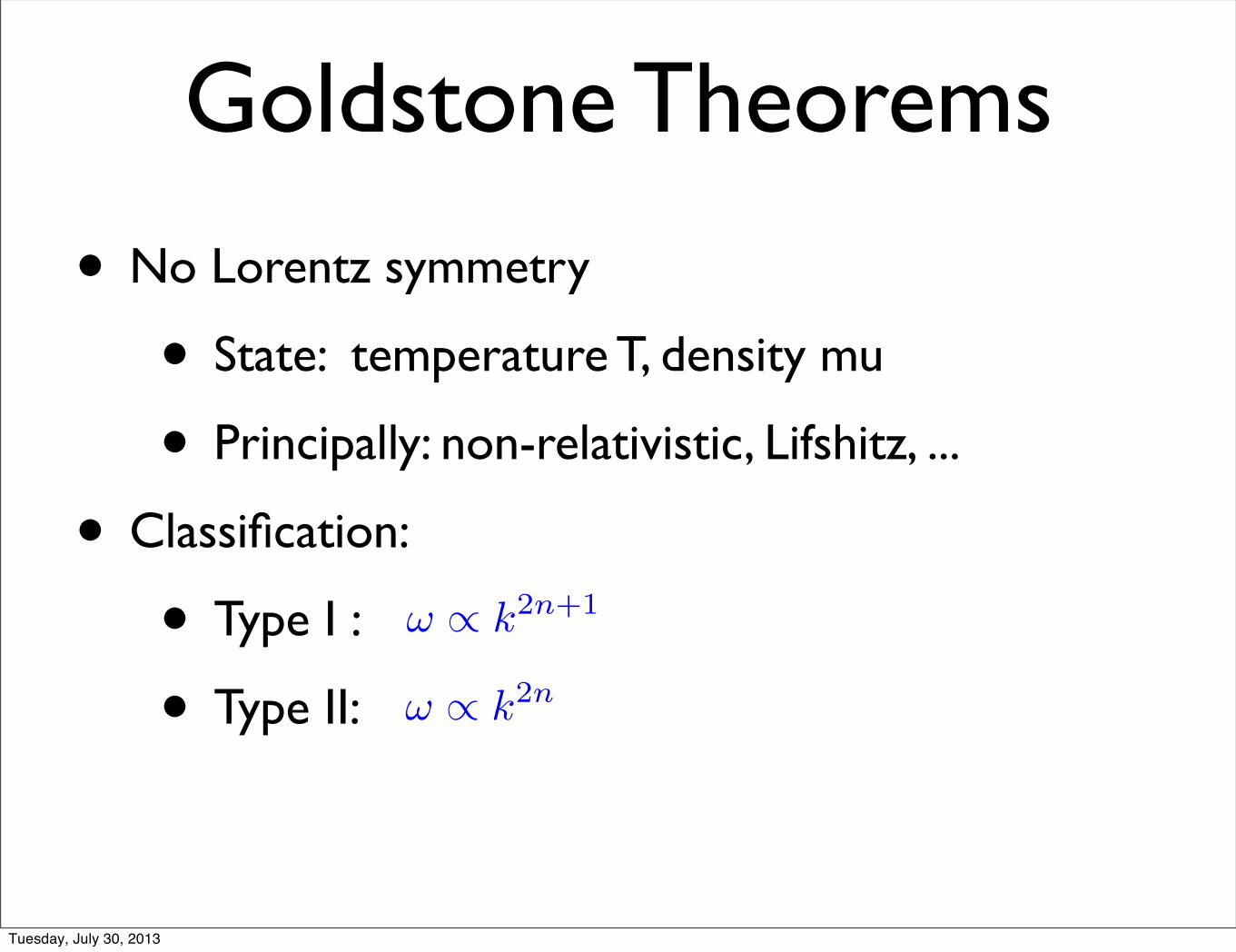
Goldstone Theorems

• No Lorentz symmetry

• State: temperature T, density mu

• Principally: non-relativistic, Lifshitz, ...

• Classification:

• Type I :

• Type II:

ω ∝ k2n+1

ω ∝ k2n


Goldstone Counting• Chadha-Nielsen

• Brauner-Watanabe-Murayama

• Brauner-Murayama-Watanabe, Nicolis-Piazza, Kapustin(“massive” Goldstone)

[Qa, Qb] = Bab

NI +NII = NBG − 1

2rank(Bab)

ω = qµ

NI + 2NII ≥ NBG


Field Theory ModelT. Schafer, D. T. Son, M. A. Stephanov, D. Toublan and J. J. M. Verbaarschot, [hep-ph/0108210]

V. A. Miransky and I. A. Shovkovy, [hep-ph/0108178]

L = (∂0 − iµ)Φ†(∂0 + iµ)Φ− ∂Φ†∂Φ−M2Φ†Φ− λ4(Φ†Φ)2

φ = (φ1,φ2)T Doublet of U(2)

ω21 =

µ2 −M2

3µ2 −M2p2 +O(p4) ,

ω22 = 6µ2 − 2M2 +O(p2) ,

ω23 = p

2 − 2µω3 ,

ω24 = p

2 + 2µω4 .

φ = (0, v)T

Type I Goldstone

ω3 ≈ p2

2µType II Goldstone

ω4 = 2µ “Massive Goldstone”


Holography • Global on boundary = local in Bulk

• U(2) gauge fields + scalar in doublet

• gauged model,

• Chemical potential only in U(1)

• Holographic Goldstone modes = Quasinormal Modes

• Simplest: U(2) generalization of HHH(Hartnoll-Herzog-Horowitz)

• Decoupling limit


Holography

!3 !2 !1 0 1 2 3!5

!4

!3

!2

!1

0

Re!Ω"

Im!Ω"

O1Theory

!3 !2 !1 0 1 2 3!6

!5

!4

!3

!2

!1

0

Re!Ω"

Im!Ω"

O2 Theory

Figure 2: Lowest scalar quasinormal frequencies as a function of the temperature and at momen-tum k = 0, from T/Tc = ∞ to T/Tc = 0.81 in the O2 theory (right) and to T/Tc = 0.56 in the O1

theory (left). The dots correspond to the critical point T/Tc = 1 where the phase transition takesplace. Red, blue and green correspond to first, second and third mode respectively.

−2.545+0.825i in the O2 theory and R1(Tc) = 0.686− 0.348i in the O1 theory. In general,

one expects the residues of hydrodynamic modes that correspond to conserved quantities

of the system to vanish in the limit of zero momentum, since its susceptibility remains

constant. Consider for instance the diffusion mode associated to conserved density. The

susceptibility is defined through the two point correlation function as

χ = limk,ω→0

〈ρρ〉 = limk,ω→0

iσk2

ω + iDk2=

σ

D, (3.26)

where D is the diffusion constant and σ is the conductivity. The residue, iσk2, vanishes and

one recovers the well-known Einstein relation σ = Dχ. However, for hydrodynamic modes

appearing at second order phase transitions the order parameter susceptibility should di-

verge at the critical point. This order parameter susceptibility is given in our case by the

correlator of the boundary operator sourced by the scalar field. At the critical temperature

it is

χOiOi= lim

k,ω→0〈OiOi〉 = lim

k,ω→0

Ri(k, Tc)

ω − ωH(k, Tc)→ ∞ (3.27)

since ωH(0, Tc) = 0 while the residue remains finite. This result allows us to identify the

lowest scalar quasinormal mode in the unbroken phase with the Goldstone boson appearing

at the critical point.

In the model under consideration one can also compute the gauge field fluctuations

in the normal phase. Nevertheless, as the model does not include the backreaction of

the metric, the computation is not sensitive to temperature anymore. This can be seen

from the equations of motion (3.2) of the gauge fluctuations, that do not depend on the

background solutions thus are independent of the temperature. Hence we recover the

results for the quasinormal modes of vector field perturbations in the AdS4 black hole

background computed by [34]. For our purposes the most important fact is the presence

– 13 –

Normal phase (high T) I. Amado, M. Kaminski and K. L., [arXiv:0903.2209 [hep-th]]

also4 Diffusion

modesω = −iDk2


Holography Broken phase, Type I (4th sound) ω = vsk + (b− iΓs)k

2

small and subleading compared to the linear term that determines the speed of sound. In[15] this real quadratic part has not been studied.

0.2 0.4 0.6 0.8 1.0TTc

0.2

0.4

0.6

0.8

vs2

0.5 0.6 0.7 0.8 0.9 1.0TTc

0.00

0.05

0.10

0.15

0.20

0.25

0.30

0.35s

Figure 4: Speed of sound and damping for the sound mode. The speed of sound goes tozero at the critical temperature. The damping constant first rises quickly and then falls offagain. Precisely at the critical temperature its value is such that the sound modes connectcontinuously to the scalar modes that become massless there. The peak in the dampingconstant sits close to the critical temperature and was not resolved in [15].

For very small temperatures the velocity approaches its conformal value v2s = 1/2 whilethe width goes to zero, see figure 4. Close to the phase transition, the speed of sound has amean field behavior as a function of temperature

v2s ≈ 2.8

1− T

Tc

. (42)

As expected, at T = Tc the speed of sound vanishes. This can be traced back to the factthat at the phase transition the total mass m2

∗ = M2 − µ2 fulfills m2∗ = v2 = 0, as expected,

and hence the complex scalar field, charged under a U(1) symmetry, becomes massless.Indeed, one can write down the effective action, analogous to (4), for a complex scalar

field with mass M , in the presence of a chemical potential for a U(1) symmetry that isspontaneously broken. The excitations on top of the U(1)-breaking background have adispersion relation equal to (8)-(9), being (8) the type I Goldstone boson. It is a generalfeature of these linear sigma models that the coefficient in front of the linear term in themomentum depends on m2

∗, as can be explicitly checked for the case at hand (see (8)).Therefore, at the phase transition the leading term in the dispersion relation is of O(k2);this effect can be seen very clearly with numerical methods, as shown in Figure 5. Sincethe quasinormal mode spectrum has to vary continuously through the second order phasetransition the real and complex coefficients of the k2 term have to coincide at T = Tc withthe ones obtained from the massless scalars in the unbroken phase. Numerically we findb(Tc) = 0.22 and Γs(Tc) = 0.071.

Pseudo diffusion mode: In the unbroken phase our model has only one hydrodynamicmode, the diffusion mode ω = −iDk2 + O(k4) with D = 3/(4πT ) in physical units. The

14


Holography Broken phase, Type II ω = (B − iC)k2

The temperature dependence of B and C is plotted in Figure 18. The value at T = Tc is

given by the same value as in the ungauged model (46) and in fact can also be cross checked

by calculating the scalar mode dispersion relation in the unbroken phase at T = Tc since

the QNMs must be continuous through the phase transition. We find a rather surprising

dependence of B with the temperature. It starts at a finite value at the transition and then it

rises rather sharply and falls off slower. It reaches a minimum at T ≈ 0.49Tc, temperature at

which we found the change of sign in the residue of current-current correlators. We also find

another peak around T ≈ 0.4Tc. We expect that it is again related with the instability found

in the gauge sector around that temperature. It would also be interesting to calculate B(T )using an alternative method e.g. as the sound velocity can be calculated from thermodynamic

considerations alone. In order to do this one would need to formulate the hydrodynamics of

type II Goldstone modes. We are however not aware of such a hydrodynamic formulation

and leave this for future research.

0.3 0.4 0.5 0.6 0.7 0.8 0.9 1.0TTc

0.0

0.5

1.0

1.5

2.0BT

0.3 0.4 0.5 0.6 0.7 0.8 0.9 1.0TTc

0.00

0.02

0.04

0.06

0.08

0.10

0.12

0.14

CT

0.996 0.997 0.998 0.999 1.000TTc

0.00

0.02

0.04

0.06

0.08

0.10

0.12

0.14CT

Figure 18: B (left) and C (right) as a function of T/Tc. The zoom-in shows the peak of Cclose to the transition. Furthermore at T 0.4Tc a sharp peak shows up in both coefficients.

We relate this feature also to the instability arising in the vector sector.

The attenuation C(T ) decreases rapidly with temperature. For temperatures T/Tc < 0.9it is negligible and the width of the type II Goldstone scales with k4

in the hydrodynamic

limit. This fast decreasing with temperature reflects that this mode propagates almost ideally

in the fluid at low temperature. No further ungapped modes can be found in this sector.

4.6.2 Higher quasinormal modes

Higher quasinormal modes correspond to gapped modes in the QNM spectrum and thus

represent subleading contributions to the low energy Green’s functions. We will focus here

only on two of them: the continuation of the two diffusive modes of the unbroken phase and

the special gapped mode that appears as the partner mode of the type II Goldstone mode

in the field theoretical model.

33


Holography Broken phase, Type II ω = (B − iC)k2

The temperature dependence of B and C is plotted in Figure 18. The value at T = Tc is

given by the same value as in the ungauged model (46) and in fact can also be cross checked

by calculating the scalar mode dispersion relation in the unbroken phase at T = Tc since

the QNMs must be continuous through the phase transition. We find a rather surprising

dependence of B with the temperature. It starts at a finite value at the transition and then it

rises rather sharply and falls off slower. It reaches a minimum at T ≈ 0.49Tc, temperature at

which we found the change of sign in the residue of current-current correlators. We also find

another peak around T ≈ 0.4Tc. We expect that it is again related with the instability found

in the gauge sector around that temperature. It would also be interesting to calculate B(T )using an alternative method e.g. as the sound velocity can be calculated from thermodynamic

considerations alone. In order to do this one would need to formulate the hydrodynamics of

type II Goldstone modes. We are however not aware of such a hydrodynamic formulation

and leave this for future research.

0.3 0.4 0.5 0.6 0.7 0.8 0.9 1.0TTc

0.0

0.5

1.0

1.5

2.0BT

0.3 0.4 0.5 0.6 0.7 0.8 0.9 1.0TTc

0.00

0.02

0.04

0.06

0.08

0.10

0.12

0.14

CT

0.996 0.997 0.998 0.999 1.000TTc

0.00

0.02

0.04

0.06

0.08

0.10

0.12

0.14CT

Figure 18: B (left) and C (right) as a function of T/Tc. The zoom-in shows the peak of Cclose to the transition. Furthermore at T 0.4Tc a sharp peak shows up in both coefficients.

We relate this feature also to the instability arising in the vector sector.

The attenuation C(T ) decreases rapidly with temperature. For temperatures T/Tc < 0.9it is negligible and the width of the type II Goldstone scales with k4

in the hydrodynamic

limit. This fast decreasing with temperature reflects that this mode propagates almost ideally

in the fluid at low temperature. No further ungapped modes can be found in this sector.

4.6.2 Higher quasinormal modes

Higher quasinormal modes correspond to gapped modes in the QNM spectrum and thus

represent subleading contributions to the low energy Green’s functions. We will focus here

only on two of them: the continuation of the two diffusive modes of the unbroken phase and

the special gapped mode that appears as the partner mode of the type II Goldstone mode

in the field theoretical model.

33

additional unstable mode: p-wave condensate


Holography Conductivities related to type I

We see that the resulting system of equations is now completely decoupled. We only havetwo diagonal conductivities σ++ and σ−−, corresponding to the unbroken U(1) diffusivesector and a mode which is associated to the broken U(1) coupling to the condensate. Theformer is the same as in the unbroken phase and of no further interest for us. The latteris again the well-studied U(1) s-wave superconductor. Its conductivity has been alreadycalculated in [3]. To check our numerics we have re-calculated it and in Figure 11 we showits behavior. It coincides completely with [3]. The real part shows the ω = 0 delta functioncharacteristic of superconductivity9. Numerically this can be seen through the 1/ω behaviorin the imaginary part. The Kramers-Kronig relation (see (121) in appendix A) implies theninfinite DC conductivity. The real part of the AC conductivity also exhibits a temperaturedependent gap.

0 2 4 6 8 10Ω0.0

0.2

0.4

0.6

0.8

1.0

1.2

ReΣ

2 4 6 8 10Ω

1

0

1

2

3

4

5

ImΣ

Figure 11: Real part (left) and imaginary part (right) of the conductivity as a function offrequency. The plots correspond to temperatures in the range T/Tc ≈ 0.91− 0.41, from redto purple. As expected, the plots reproduce the ones of [3].

4.5 Conductivities in the (1)− (2) sector

The relevant equations for the (1)− (2) sector read

0 = fa(1)x + f a(1)x +

ω2

f−Ψ2 +

Θ2

f

a(1)x − 2i

Θω

fa(2)x , (97)

0 = fa(2)x + f a(2)x +

ω2

f−Ψ2 +

Θ2

f

a(2)x + 2i

Θω

fa(1)x . (98)

These equations obey the symmetry

(a(1)x → a(2)x , a(2)x → −a(1)x ) . (99)

9In general, this behavior is also typical of translation invariant charged media, in which accelerated

charges cannot relax. However, working in the probe limit we effectively break translation invariance and

therefore the infinite DC conductivity is a genuine sign of superconductivity.

27


Holography Conductivities related to type II, diagonal

Superconductor !

1 2 3 4 5Ω

4

2

0

2

4

6

8

10ReΣ11

1 2 3 4 5Ω

4

2

0

2

4

6

8

10ImΣ11


Holography Fate of the diffusion modes in broken phase

ω = −iγ − iDk2U(1) sector: gapped (pseudo) diffusion

0.1 0.2 0.3 0.4 0.5k

0.5

0.4

0.3

0.2

0.1

0.0Im Ω

0.70 0.75 0.80 0.85 0.90 0.95 1.00

T

Tc

0.2

0.4

0.6

0.8

1.0

1.2

Γ

Figure 6: (Left) Dispersion relation of the gapped pseudo diffusion mode in the broken phasefor three different temperatures. The gap widens as the temperature is lowered. (Right) Gapγ as a function of the reduced temperature T/Tc. As one approaches the critical temperaturefrom below the gap vanishes linearly.

density or x-component of the current.

2 4 6 8ReΩ

6

5

4

3

2

1

ImΩ

0.6 0.7 0.8 0.9 1.0

T

Tc

1.5

1.0

0.5

0.0Im Ω

Figure 7: (Left) Continuation of the second and third scalar QNM into the broken phase.The real part grows as the temperature is lowered whereas the imaginary part shows verylittle dependence on T . (Right) The gap γ (blue line) and the imaginary part of the lowest(scalar) mode fluctuation (red line) in the broken phase are shown as function of T/Tc.At T∗ ≈ 0.69Tc the imaginary parts cross. For lower temperatures the late time responseis not dominated anymore by the pseudo diffusion mode and consequently is in form of aexponentially decaying oscillation.

For finite momentum the response pattern is expected to be different however. Now onealso has to take into account the sound mode. While precisely at zero momentum the soundmode, i.e. the Goldstone mode, degenerates to a constant phase change of the condensate atsmall but non-zero momentum the long time response should be dominated by the complexfrequencies (42). If one looks however only to the response in the gauge invariant orderparameter |O| the Goldstone modes, being local phase rotations of the order parameter, are

17


Holography Fate of the diffusion modes in broken phase

ω = −iγ − iDk2U(1) sector: gapped (pseudo) diffusion

0.1 0.2 0.3 0.4 0.5k

0.5

0.4

0.3

0.2

0.1

0.0Im Ω

0.70 0.75 0.80 0.85 0.90 0.95 1.00

T

Tc

0.2

0.4

0.6

0.8

1.0

1.2

Γ

Figure 6: (Left) Dispersion relation of the gapped pseudo diffusion mode in the broken phasefor three different temperatures. The gap widens as the temperature is lowered. (Right) Gapγ as a function of the reduced temperature T/Tc. As one approaches the critical temperaturefrom below the gap vanishes linearly.

density or x-component of the current.

2 4 6 8ReΩ

6

5

4

3

2

1

ImΩ

0.6 0.7 0.8 0.9 1.0

T

Tc

1.5

1.0

0.5

0.0Im Ω

Figure 7: (Left) Continuation of the second and third scalar QNM into the broken phase.The real part grows as the temperature is lowered whereas the imaginary part shows verylittle dependence on T . (Right) The gap γ (blue line) and the imaginary part of the lowest(scalar) mode fluctuation (red line) in the broken phase are shown as function of T/Tc.At T∗ ≈ 0.69Tc the imaginary parts cross. For lower temperatures the late time responseis not dominated anymore by the pseudo diffusion mode and consequently is in form of aexponentially decaying oscillation.

For finite momentum the response pattern is expected to be different however. Now onealso has to take into account the sound mode. While precisely at zero momentum the soundmode, i.e. the Goldstone mode, degenerates to a constant phase change of the condensate atsmall but non-zero momentum the long time response should be dominated by the complexfrequencies (42). If one looks however only to the response in the gauge invariant orderparameter |O| the Goldstone modes, being local phase rotations of the order parameter, are

17

Keep in mind, please


Holography Fate of the diffusion modes in broken phasenon-Abelian sector: 2 gapped modes ω = ±Ω− iΓ

6 4 2 2 4 6ReΩ

0.5

0.4

0.3

0.2

0.1

ImΩ

T0.8Tc

T0.5Tc

Figure 19: Imω versus Reω at k = 0 as a function of the temperature. The shape of the

figure is compatible with T symmetry, since there are two pseudo-diffusive modes. Having

Reω(k = 0) = 0 is characteristic of the non-Abelian case.

0.80 0.85 0.90 0.95 1.00TTc

0.0

0.1

0.2

0.3

0.4

0.5

0.6

0.7Re MT

0.80 0.85 0.90 0.95 1.00TTc

1.2

1.0

0.8

0.6

0.4

0.2

0.0Im MT

Figure 20: Real (left) and imaginary (right) part of M(T ) as a function of T/Tc. As the

temperature approaches Tc, the value of M(T ) reaches the one prescribed by continuity

through the phase transition.

35


Holography “Massive” Goldstone

expected for second order phase transitions, however instead of simply developing an imag-inary gap to drop out of the hydrodynamic spectrum as for the usual U(1) superconductor,they pair up in two modes that on top of this gap also develop a real part.

The fact that Re(ω) does not vanish for these modes implies that sufficiently close toTc and in the limit k = 0, the late-time response of the perturbed state will present anoscillatory decay of the perturbations, meaning that, contrary to the U(1) case, there willnot be a temperature at which the late-time behavior changes qualitatively.

Special Gapped mode: Seeking for this mode is computationally much more involved.Its behavior is characterized by a gap that is proportional to µ. In particular, in [31] it wasargued that a type II Goldstone mode is accompanied by a gapped mode obeying ω(0) = qµwith q being the charge of the corresponding field. In our conventions here we have q = 1.So we have to look for a mode with ω(k = 0) = µ. Furthermore we expect that it connectsto the lowest mode of the complex conjugate scalar in the unbroken phase.

In Figure 21 we depict such mode at zero momentum with respect to the chemical po-tential µ in numerical units. Notice that the mode is continuous at the phase transition, asexpected. We observe the linear behavior with the chemical potential that is predicted the-oretically, at least near µc. It is very difficult to do the analysis when µ > 6 due to the highcomputational power demanded to carry out the computation. The mode shows of coursealso a non-vanishing imaginary part which is due to the dissipation at finite temperature.We find that the real part above the phase transition can be approximated by

Reω = 1.10 µ near µc . (108)

This result shows a deviation from the conjectured behavior which could nevertheless bedue to uncertainties in the numerics. Let us emphasize here that the numerics involved intracking this mode through the phase transition were rather challenging.

0.5 1.0 1.5Μ Μ c

1

2

3

4

5

6

7

ReΩ0.5 1.0 1.5

Μ Μ c

6

5

4

3

2

1

ImΩ

Figure 21: Real (left) and imaginary (right) part of the special gapped mode versus thechemical potential. We encounter the expected linear behavior with µ. The plot covers boththe unbroken (dashed line) and the broken (solid line) phases.

36

Re(ω) ≈ 1.1qµ


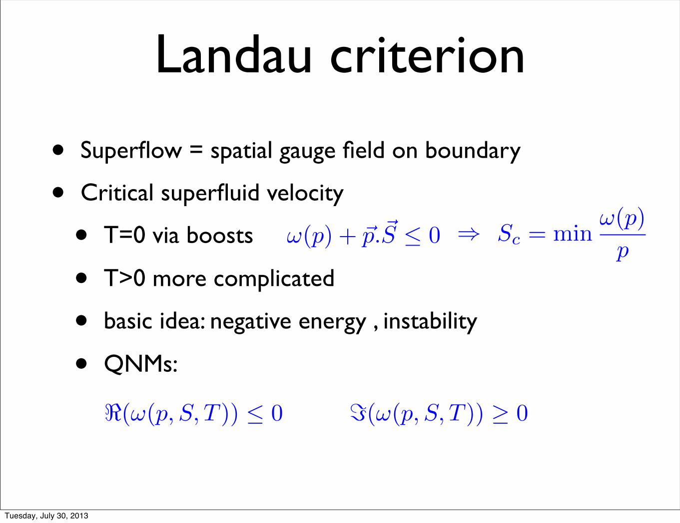
Landau criterion

• Superflow = spatial gauge field on boundary

• Critical superfluid velocity

• T=0 via boosts

• T>0 more complicated

• basic idea: negative energy , instability

• QNMs:

ω(p) + p.S ≤ 0

(ω(p, S, T )) ≤ 0 (ω(p, S, T )) ≥ 0

Sc = minω(p)

p⇒


Landau criterionType I Goldstone

0.2 0.1 0.1 0.2

0.15

0.10

0.05

0.05

0.10

0.15

Γ

0.5 0.5vs

0.6

0.4

0.2

0.2

0.4

0.6

vs

Γ


Landau criterionWeak Coupling

(courtesy: A. Schmitt) [Alford, Mallavarpu, Schmitt, Stetina] to appear

0.5 0.0 0.5

0.5

0.0

0.5


Landau criterionType I Goldstone

0.2 0.4 0.6 0.8 1.0k

0.06

0.04

0.02

0.00

0.02Im Ω

0.2 0.4 0.6 0.8 1.0k0.05

0.00

0.05

0.10

0.15

0.20Re Ω

Stripes?


Drude Peak

2 4 6 8 10 12Ω0.0

0.2

0.4

0.6

0.8

1.0

Re Σ03

2 4 6 8 10Ω

2

4

6

8

10

12Im Σ03

Due to gapped “Pseudo” diffusion mode !


Landau criterionType II Goldstone

0.5 1.0 1.5 2.0k

0.3

0.2

0.1

0.0

0.1

0.2

0.3

Re Ω

0.5 1.0 1.5 2.0k

0.05

0.00

0.05

0.10Im Ω

Figure 9: Real and Imaginary parts of the dispertion relation of the lowest QNM of the

(1)-(2) sector in the gauged model. Both plots correspond to fixed Sx/µ = 0.15 and a regime

of temperatures from T = T = 0.95Tc (red) to T = 0.45Tc (blue). Lower temperatures show

analogue behaviour. XXHay que hacer algunas curvas mas smooth, (lineas rojas

cerca de k parte real)XX

(10), where (ω(k)) is ploted against the momentum k at a fixed supervelocity Sx/µ = 0.25and for a long range of temperatures. Hence, we conclude that the gauge sector has the

effect of incresing the value of the maximum momentum.

5 Conclusions

We have analyzed the holographic realization of the Landau criterion of superfluidity.

The study was motivated by the appearance of Type-II NG bosons in the model (5), as

detailed in [2], which, according to the aforementioned criterion, should be responsible for

driving the system out of the superfluid phase for arbitrarily small supervelocity.

Taking advantage of the fact that the usual U(1) holographic s-wave superconductor is

contained in (5), we have revisited the Landau criterion for holographic Type-I NG bosons

in Section 3, pointing out that, when adressing the problem of the stabily of the superfluid

at finite supervelocity Sx/µ, the analysis of the free energy does not give the correct answer.

The QNM spectrum presents a tachyon at finite momentum for temperatures T ∗ < T < T ,being T the temperature at which the system is supossed to pass through a phase transition

to an homogeneous and stable superfluid with non-vanishing supervelocity according to the

F.E. calculation. Hence, the homogeneous superfluid is stable only for T < T ∗, see Figure

(6). The results of the velocity of sound vs. the angle γ between the momentum and the

supervelocity, depicted in Figures (3) and (4), are perfectly consistent with this statement:

at T = T ∗and γ = π the velocity of sound vanishes. This condition can be easily seen to

be equivalent to the Landau criterion and signals the existence of a critical velocity above

which the superfluid is not stable anymore. Indeed, in the simple language of Section 1, the

dispersion relation from the moving frame can be written as

17

Does not support finite superflow!Superconductor but not Superfluid


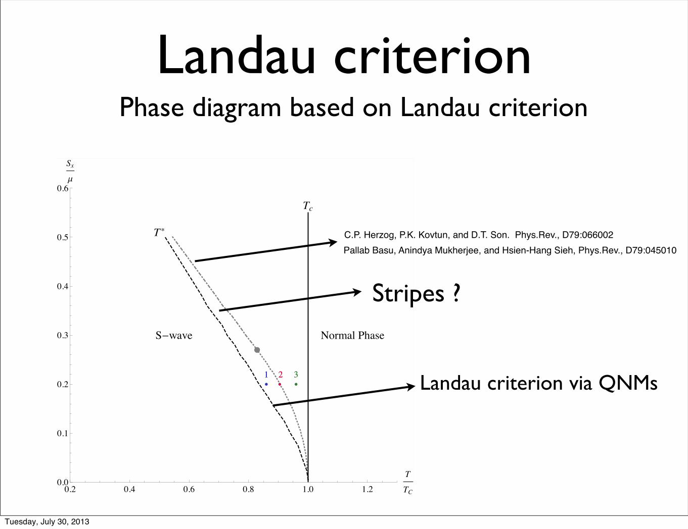
Landau criterionPhase diagram based on Landau criterion

11 22 33

0.2 0.4 0.6 0.8 1.0 1.2

T

TC0.0

0.1

0.2

0.3

0.4

0.5

0.6

SxΜ

T

Tc

Swave Normal Phase1N1N

2N,S2N,S

3N3N

1S1S

0.5 1.0 1.5 2.0k

0.10

0.05

0.00

0.05

0.10Im Ω

Figure 6: Left: Phase Space after the study of the QNM’s. Grey line corresponds to T ,the transition temperature found by direct analysis of the F.E.. At a certain point (Disk)the transition changes from 2nd order (dotted) to 1st order (dash-dotted). Black solid linecorresponds to the critical temperature in abscence of superfluid velocity. The black dashedline corresponds to T ∗, the temperature the local instability appears at. Points 1,2 and 3indicate the values of tamperature and velocity used in the r.h.s. plot. Right: Imaginarypart of ω of the lowest QNM for different temperatures (see l.h.s. plot) and fixed Sx/µ = 0.2.Dashed lines were obtained in the Normal Phase whereas solid lines were calculated in theS-wave phase.

Therefore the QNM results indicate that at finite momentum the phase transition (fromlow to high temperatures) occurs actually at a lower temperature T ∗ < T . Similarly, if weimagine the system at fixed temperature and start rising the supervelocity, both vs and Γwill vanish at some value of Sx/µ, which we claim is indeed the critical velocity vc of thesuperfluid, in the sense of the Landau criterion.

As a remarkable fact, the imaginary part exhibiting the instability has a maximum atfinite momentum as well, which suggests that the stable intermediate phase might be a spa-tially inhomogeneous phase.

Recall that the Landau criterion can be formulated uniquely in terms of (ω). At agiven temperature the critical velocity corresponds to vs = 0 or equivalently the value ofSx/µ where (ω) becomes negative (see Figure (5)). That the criterion is a statement about(ω) reflects the fact that it holds also at zero temperature. Remarkable enough, at finitetemperature the dispersion relation of the gapless mode gets itself altered due to both thesupervelocity and the temperature ([1], [13]), implying that generically the critical value ofSx/µ at fixed temperature does not correspond to the velocity of sound of the Goldstonemode at the same temperature and vanishing supervelocity.

An extra comment is in order here regarding the space between Tc and T in the l.h.s.of Figure (6). The fact that the lowest QNM is unstable in this regime (see line 2N,S in

12

C.P. Herzog, P.K. Kovtun, and D.T. Son. Phys.Rev., D79:066002Pallab Basu, Anindya Mukherjee, and Hsien-Hang Sieh, Phys.Rev., D79:045010

Landau criterion via QNMs

Stripes ?


Summary • QNMs rule !

• Compare to weak coupling

• Universality of Pseudo-diffusion ?

• “Un-gauged” model: no SU(2) gauge fields, violates some Theorems

• Backreacted models1st, 2nd, 4th sound modes etc.

• Striped phases ?

• Many beautiful plots ...

[Mark G. Alford, S. Kumar Mallavarapu, Andreas Schmitt, and Stephan Stetina, arXiv:1212.0670]

0.2 0.1 0.1 0.2

0.2

0.1

0.1

0.2

Γ


Holography Conductivities related to type II, off-diagonal

no Superconductor !of frequency. At T/Tc = 1 the system is practically decoupled, so for all temperatures the

off-diagonal conductivity goes to zero as ω increases.

2 4 6 8 10 12 Ω0

1

2

3

4

5

ReΣ 12

2 4 6 8 10 12 Ω

3

2

1

0

1

2

3

4

ImΣ 12

Figure 14: Real (left) and imaginary (right) part of σ12 as a function of ω for T/Tc ≈0.91− 0.41, from red to purple.

Observe that σ12(ω) behaves as a normal conductivity. Its real part vanishes as ω → 0,

whereas the imaginary part tends to a constant value.

4.5.3 Conductivities σ+− and σ−+

It is worth to notice that the equations (97)-(98) decouple if we define a new vector field

ϕ =

A+

A−

=

1 i1 −i

a(1)x

a(2)x

= S ϕ . (102)

In this basis, the equations of motion become

0 = fA± + f A

± +

(ω ∓Θ)2

f−Ψ2

A± . (103)

It is easy to check that the relation between the conductivity matrices in the two basis is

given by

σ =ST

−1σS−1 , (104)

and that only the off-diagonal components of σ are non vanishing.

The conductivities σ−+ and σ+− are represented in Figure 15 and 16, respectively. The

plot of the conductivity σ−+ is particularly suggestive. Besides the superconducting delta

of the DC conductivity, it resembles the behavior observed in Graphene [29]. Such a resem-

blance of the conductivities of holographic superconductors to the one of graphene has been

pointed our already in [37]. We emphasize however that the conductivities shown in figure

15 have an even closer resemblance to [29]. In particular, at small frequencies we see that

30


karl landsteiner - mpp theory group

Documents