karhunen-loeve procedure for gappy data · r. everson and l. sirovich vol. 12, no. 8/august 1995/j....

R. Everson and L. Sirovich Vol. 12, No. 8 /August 1995 /J. Opt. Soc. Am. A 1657

Karhunen–Loeve procedure for gappy data

R. Everson and L. Sirovich

The Rockefeller University, New York, New York 10021-6399

Received November 14, 1994; revised manuscript received March 14, 1995; accepted March 29, 1995

The problem of using the Karhunen–Loeve transform with partial data is addressed. Given a set of empiricaleigenfunctions, we show how to recover the modal coefficients for each gappy snapshot by a least-squaresprocedure. This method gives an unbiased estimate of the data that lie in the gaps and permits gaps to befilled in a reasonable manner. In addition, a scheme is advanced for finding empirical eigenfunctions fromgappy data. It is shown numerically that this procedure obtains spectra and eigenfunctions that are closeto those obtained from unmarred data.

1. INTRODUCTIONA primary purpose of this paper is to address the followingquestion: How much image information is necessary forthe restoration of a full image from a partial image, if itis known that the image belongs to a certain well-definedclass of images? (Alternatively, how much degradation,by deletion of pixels, can such an image suffer and still berecovered?) Such questions are prompted by a numberof applications in which image information is collectedas an ensemble of like images and, owing to technicalor natural circumstances, some or all of the images aremarred by gaps in the data. Many examples of this sortoccur for data gathered from remote-sensing satellites.As an illustration we mention the presence of cloud coveras a natural obstruction that leaves gaps in data records.1

Although the language and illustrations presented herecome from image analysis, the methodologies apply tothe wider arena of databases having support in higherdimensions. Although our deliberations may be relevantto image compression, this subject is not pursued here.

First we address the problem of recovering a full im-age from a marred image when the properties of an en-semble of like images are known. The methods rely onthe Karhunen–Loeve (K–L) expansion for the ensemble,and in Section 2 we address the problem of finding the(K–L) expansion from a marred ensemble.

In order to deal with the issues involved, we reconsiderthe Rogues’ Gallery problem, which was formulated andsolved in Refs. 2 and 3. Briefly stated, this is the prob-lem of analyzing an ensemble of images of human faces.A snapshot of a face will be denoted f fsxd, where f

represents the deviation in gray level from the ensemblemean gray level at pixel location x sx, yd. If the facesare indexed by n, the ensemble is denoted hfnj, where1 # n # N , and N represents the number of faces in theensemble. Normalization and other related details maybe found in Refs. 2 and 3. It was shown there that thereexists an optimal representation in the sense that the av-erage error,

e

*áf 2

MPn1

ancnsxd

á 2+, (1)

is minimal for all M . Here k?k2 denotes the usual L2

0740-3232/95/081657-08$06.00

norm and k?l denotes the average over the ensemble. Theminimal value of e is obtained if the basis elements cn

satisfy the eigenfunction problem,

ZKsx, y dcns y ddy lncnsxd , (2)

scn, cmd Z

cnsxdcmsxddx dnm , (3)

where

Ksx, y d kfsxdfsy dl 1N

NXn1

fsxdfsy d (4)

is the two-point correlation function. This is the essenceof the K–L procedure or principal components analy-sis, also known under a variety of other designations,and yields to standard numerical procedures. In whatfollows, hcnsxdj, which appears as eigenfunctions of thecorrelation operator, will be referred to as the empiricaleigenfunctions. The K–L procedure and variations of ithave been rediscovered a number of times. A modernform of it goes back to Schmidt.4 (For a description andextension see Sirovich and Everson.5) Stewart6 has re-cently reviewed the history of the method, and a review ofits use in turbulence theory was made by Berkooz et al.7

Turk and Pentland8 subsequently made calculations simi-lar to those presented in Refs. 2 and 3 and used empiri-cal eigenfunctions for face recognition. O’Toole et al.9,10

used empirical eigenfunctions to investigate perceptionof race and sex.9,10 A related application to an oceano-graphic problem has been presented by Kelly.11

2. MARRED FACESWith the use of the empirical eigenfunctions, cn, whichhere we may call eigenfaces, only a relatively small num-ber of parameters enter into the specification of a par-ticular face. In quantitative terms it was found that onaverage 50 eigenfaces account for approximately 93% ofthe variance based on departures from the mean2 fora description of the ensemble and normalization. Thisshould be compared with the O(104) gray levels requiredfor specification of each snapshot.

1995 Optical Society of America

1658 J. Opt. Soc. Am. A/Vol. 12, No. 8 /August 1995 R. Everson and L. Sirovich

This result implies that for a face fsxd, a suitable ap-proximation can be obtained from a limited summation,

fsxd øNP

n1ancnsxd , (5)

where the coefficients an are obtained from the usualinner product,

an sf, cnd , (6)

and N represents the number of basis functions neededto meet some specified error bound. Relation (5), lookedat in another way, states that in the presence of perfectinformation (zero noise) we need to know only the graylevels fsxd at N pixel locations.

To investigate this assertion we will consider marredfaces and then investigate how well they can be recon-structed. We express a masked face by

fsxd msxdfsxd , (7)

where m 0 on the mask and m 1 elsewhere. Thechallenge is to write fsxd in the form of relation (5),

fsxd ø msxdNP

n1ancnsxd , (8)

and from this to determine a best set of coefficients an.Once this is done we can inquire how well f is capturedby

PNn1 ancn. Part of the problem involves the choice

of N .The inner product [Eq. (6)] can no longer be used to find

the coefficients, because it requires information from thefull range of x; i.e., the fn are not necessarily orthogonalover the support of f, sffg. However, we can then usea least-squares criterion to achieve a best fit of form (5).That is, we minimize the error

E Z

sffgdx

24fsxd 2

NXn1

ancn

352

. (9)

The minimization of E leads to0@f 2NP

n1ancn, ck

1Asffg

0 , (10)

which requires that the residual be orthogonal to ck fork 1, . . . , N , where as indicated the inner product is overthe support of f, sffg. The Hermitian matrix

Mkn sck, cndsffg (11)

is nonnegative and is in principle OsN d.If we write

fk sf, ckdsffg , (12)

then in vector notation we seek the unknown coefficientsak from

Maaa f . (13)

In the event that sffg is sufficiently dense in the space,then M ø I, which among other properties says that the

eigenvalues of M are close to unity, and ak ø sf, ckdsffg.In the present instance, if we denote the eigenvalues mn

and the corresponding orthonormal eigenvectors vn, thesolution to Eq. (13) is then given by

aaa NP

k1

1mn

svn, fdvn . (14)

Thus on intuitive grounds the construction becomes ques-tionable if the mk depart significantly from unity; this ismade explicit in Appendix A.

To illustrate the nature of this construction, we con-sider the mask shown in Fig. 1a. This is a relativelyextreme mask that obscures 90% of the pixels in a ran-domly chosen way. This was used to mask a face that didnot belong to the original ensemble that was used to de-termine the eigenfunctions. The result of applying theabove procedure, finding the a from Eq. (13) and usingN 50 eigenfunctions, is shown in Fig. 1b. The origi-nal unmasked face is shown in Fig. 1c, and the projectionof the original face onto 50 eigenfunctions is shown in

Fig. 1. Reconstruction of a face, not in the original ensemble,from a 10% mask. The reconstructed face, b, was determinedwith 50 empirical eigenfunctions and only the white pixels shownin a. The original face is shown in c, and a projection (with allthe pixels) of the face onto 50 empirical eigenfunctions is shownin d.


Fig. 2. Reconstruction of a face from a 10% mask. The recon-structed face b was determined with 50 empirical eigenfunctionsand only the white pixels shown in a. The original face, whichwas a member of the original ensemble, is shown in c and aprojection (with all the pixels) of the face onto 50 empiricaleigenfunctions is shown in d.

Fig. 1d. Though the procedure does not recover the origi-nal face exactly, the construction is visually close to theprojection onto 50 eigenfunctions, which utilizes the en-tire area and is the best that may be achieved with 50functions.

We underline the fact that the masked face did notenter into the determination of the eigenfaces. When theface to be reconstructed is a member of the ensemble usedto construct the eigenfunctions, both the reconstructedface and the projected face are closer to the original.Figure 2 shows the result of a reconstruction for a facethat was a member of the original ensemble.

In carrying out this construction, we have taken N 50in Eq. (10). This, as Fig. 3 shows, is an optimal choice forthe number of fitting functions when the fraction of unob-scured pixels p 0.1. Figure 3 shows the mean squarederror,

Rjf 2

PNn1 ancnj2dx, averaged over 48 faces not

part of the original ensemble. The bottom curve corre-sponds to p 1. Here the entire face is unmasked, thecoefficients are determined by the simple inner product,and the error is the best that may be attained for a par-

ticular N , though it is necessarily larger thanP

nN11 ln.When p $ 0.2 the least-squares procedure performs wellfor all N .

In Fig. 4 we show the mean squared error versus Naveraged over the 238 faces constituting the original en-semble. The errors are significantly smaller here thanfor those shown in Fig. 3, reflecting the fact that the em-pirical eigenfunctions are optimally suited to this par-ticular ensemble. Again, the lowest curve correspondsto p 1, for which the entire face is unmasked, the coef-ficients are determined by the simple inner product, andthe error is the best that may be attained for a particu-lar N . In fact, this best error is given by

PnN11 ln.

Clearly, when p $ 0.05 the least-squares procedure per-forms well.

The basic reason for the ability of the procedure justpresented to recover the marred regions is, in part, thatone needs only a limited number of fitting functions towell approximate a full face that is suitably normalizedand satisfies other reasonable requirements. This num-ber, which might appropriately be called the dimensionof face space, is roughly 50. This estimate is greatly de-

Fig. 3. Mean squared error versus the number of fitting eigen-functions for snapshots that were not part of the original en-semble. Curves show the error for different unmasked areas,p. When p 1 the entire picture is unmasked and the meansquared error is the best that can be attained for a given numberof fitting eigenfunctions.

Fig. 4. Mean squared error versus the number of fitting eigen-functions for snapshots that were members of the original en-semble. Curves show the error for different unmasked areas,p. When p 1 the entire picture is unmasked and the meansquared error is the best that may be attained for a given numberof fitting eigenfunctions.


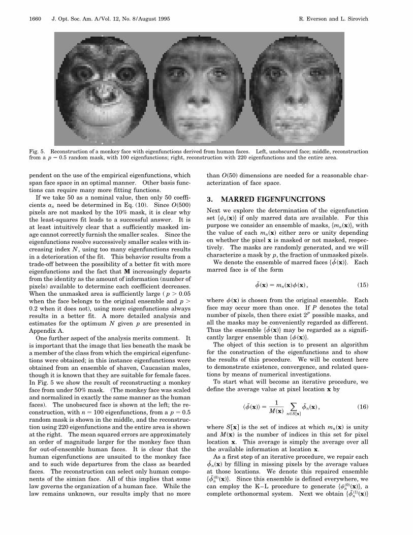
Fig. 5. Reconstruction of a monkey face with eigenfunctions derived from human faces. Left, unobscured face; middle, reconstructionfrom a p 0.5 random mask, with 100 eigenfunctions; right, reconstruction with 220 eigenfunctions and the entire area.

pendent on the use of the empirical eigenfunctions, whichspan face space in an optimal manner. Other basis func-tions can require many more fitting functions.

If we take 50 as a nominal value, then only 50 coeffi-cients an need be determined in Eq. (10). Since Os500dpixels are not masked by the 10% mask, it is clear whythe least-squares fit leads to a successful answer. It isat least intuitively clear that a sufficiently masked im-age cannot correctly furnish the smaller scales. Since theeigenfunctions resolve successively smaller scales with in-creasing index N , using too many eigenfunctions resultsin a deterioration of the fit. This behavior results from atrade-off between the possibility of a better fit with moreeigenfunctions and the fact that M increasingly departsfrom the identity as the amount of information (number ofpixels) available to determine each coefficient decreases.When the unmasked area is sufficiently large ( p . 0.05when the face belongs to the original ensemble and p .

0.2 when it does not), using more eigenfunctions alwaysresults in a better fit. A more detailed analysis andestimates for the optimum N given p are presented inAppendix A.

One further aspect of the analysis merits comment. Itis important that the image that lies beneath the mask bea member of the class from which the empirical eigenfunc-tions were obtained; in this instance eigenfunctions wereobtained from an ensemble of shaven, Caucasian males,though it is known that they are suitable for female faces.In Fig. 5 we show the result of reconstructing a monkeyface from under 50% mask. (The monkey face was scaledand normalized in exactly the same manner as the humanfaces). The unobscured face is shown at the left; the re-construction, with n 100 eigenfunctions, from a p 0.5random mask is shown in the middle, and the reconstruc-tion using 220 eigenfunctions and the entire area is shownat the right. The mean squared errors are approximatelyan order of magnitude larger for the monkey face thanfor out-of-ensemble human faces. It is clear that thehuman eigenfunctions are unsuited to the monkey faceand to such wide departures from the class as beardedfaces. The reconstruction can select only human compo-nents of the simian face. All of this implies that somelaw governs the organization of a human face. While thelaw remains unknown, our results imply that no more

than Os50d dimensions are needed for a reasonable char-acterization of face space.

3. MARRED EIGENFUNCITONSNext we explore the determination of the eigenfunctionset hcnsxdj if only marred data are available. For thispurpose we consider an ensemble of masks, hmnsxdj, withthe value of each mnsxd either zero or unity dependingon whether the pixel x is masked or not masked, respec-tively. The masks are randomly generated, and we willcharacterize a mask by p, the fraction of unmasked pixels.

We denote the ensemble of marred faces hfsxdj. Eachmarred face is of the form

fsxd mnsxdfsxd , (15)

where fsxd is chosen from the original ensemble. Eachface may occur more than once. If P denotes the totalnumber of pixels, then there exist 2P possible masks, andall the masks may be conveniently regarded as different.Thus the ensemble hfsxdj may be regarded as a signifi-cantly larger ensemble than hfsxdj.

The object of this section is to present an algorithmfor the construction of the eigenfunctions and to showthe results of this procedure. We will be content hereto demonstrate existence, convergence, and related ques-tions by means of numerical investigations.

To start what will become an iterative procedure, wedefine the average value at pixel location x by

kfsxdl 1

Msxd

Xn[Sfxg

fnsxd , (16)

where Sfxg is the set of indices at which mnsxd is unityand Msxd is the number of indices in this set for pixellocation x. This average is simply the average over allthe available information at location x.

As a first step of an iterative procedure, we repair eachfnsxd by filling in missing pixels by the average valuesat those locations. We denote this repaired ensemblehfs0d

n sxdj. Since this ensemble is defined everywhere, wecan employ the K–L procedure to generate hc s0d

n sxdj, acomplete orthonormal system. Next we obtain hfs1d

n sxdj


by fitting each fnsxd of the original ensemble by a super-position of R eigenfunctions hc s0d

n sxdj as follows: set

fs1d RP

n1as1d

n c s0dn sxd (17)

and determine the set has1dn j by minimizing the criterion

function over the pixels for which data are available; thatis, minimize

En Z

sfn 2 fs1dn d2mnsxddx . (18)

We now obtain the repaired snapshot fs1dn by filling in the

masked pixels with the fs1dn :

fs1dn sxd

8<: fnsxd if mnsxd 1fs1d

n sxd if mnsxd 0. (19)

This procedure is carried out for each fn and each mnsxd.The set hfs1d

n j is now defined everywhere and hencethrough the K–L procedure generates hc s1d

n sxdj, an ortho-normal, complete system. The iteration is now clear; wenext discuss the results.

4. RESULTSThe iteration scheme is demonstrated on an ensemble of286 faces, masked so that 40% of each face is obscured.A typical example, denoted f53sxd, is shown in Fig. 6.Each mask consists of a union of squares with randomlydistributed centers. The width of each square was drawnfrom a Poisson distribution with mean width 3 pixels.

Also shown in Fig. 6 are the intermediate snapshotsf

s1d53 , f

s2d53 , f

s5d53 , f

s10d53 , and f

s20d53 as the iteration proceeds.

At each stage the faces were repaired with R 30 eigen-

Fig. 6. 40% masked face f53 and the intermediate snapshots fs1d53 , f

s2d53 , f

s5d53 , f

s10d53 , and f

s20d53 as the iteration scheme proceeds. At

each stage the masked regions have been repaired with R 30 eigenfunctions derived from the snapshots from the preceding iteration.


Fig. 7. Eigenvalue spectrum ln after 1, 2, and 20 iterations.The solid curve shows the spectrum derived from the unmarredsnapshots.

Fig. 8. Eigenvalue spectrum ls20dn after 20 iterations compared

with the unmarred spectrum ln and the spectrum rn derivedfrom the snapshots repaired with eigenfunctions from the un-marred ensemble.

functions c skdn [see Eq. (17)]. This R was judged to be

large enough to capture the essential features of facespace but not large enough to prohibit accurate determi-nation of the asid

n .The convergence of the eigenvalue spectrum is illus-

trated in Fig. 7, which shows the principal 60 eigenval-ues ln after 1, 2, 10, and 20 iterations together withthe spectrum derived from the unmarred ensemble. Thedominant eigenvalues display a clear convergence towardthose of the unmarred spectrum. The step at index 30 isa consequence of repairing the faces with R 30 eigen-functions. In fact, since only 30 eigenfunctions are used,one cannot hope to achieve better eigenfunctions andeigenvalues than those produced by repairing (using thescheme outlined above) the marred data with 30 eigen-functions derived from perfect data. We denote theseeigenfunctions and eigenvalues xn and rn. Figure 8 com-pares the spectra from the unmarred faces, ln, from themarred faces repaired with 30 unmarred eigenfunctions,rn, and from iteration 20 of the scheme, ls20d

n . The itera-tive scheme, which lacks information about the perfecteigenfunctions, well approximates the initial portion ofthe other two spectra.

Although the eigenvalues are in good agreement, it re-mains to be checked that the eigenfunctions from the it-erative scheme approximate the eigenfunctions from the

unmarred data. Of relevance here is the convergence notof individual eigenfunctions but of the spaces spanned bygroups of eigenfunctions. Assessing the convergence ofthe eigenfunctions therefore requires a method of compar-ing subspaces. Let E and F be the projectors defining apair of subspaces, each of dimension d. Then the traceof the Hermitian matrix, Tr EFE, measures the common-ality of the subspaces. If the subspaces are identical,Tr EFE d; if they are disjoint, Tr EFE 0. We denoteCdsen, fnd the trace of EFE, where E and F are projectorsfor the subspaces spanned by the collections of vectors en

and fn. The commonality among the subspaces spannedby the first 30 unmarred eigenfunctions and the eigen-functions derived from the faces repaired with unmarredeigenfunctions is given by C30scn, xnd 29.4.

Figure 9 shows Cdsc, c skdd versus d for iterations k 1and 20. The rate of convergence is shown in Fig. 10, inwhich C30sc, c s1dd and C30s x, c s1dd are plotted against it-eration number. Even after a single iteration there isconsiderable overlap among the first seven eigenfunc-tions. The rate of convergence is initially rapid, slowingas the limit is approached. After 20 iterations there isvery good agreement between the eigenfunctions from theiteration scheme and the unmarred eigenfunctions; visu-

Fig. 9. Commonality of subspaces spanned by the unmarredeigenfunctions cn and the repaired eigenfunctions c

skdn after

k 1 and k 20 iterations.

Fig. 10. Convergence with iteration of the subspaces spannedby the repaired eigenfunctions and the unmarred eigenfunctions(squares) and the subspaces spanned by the repaired eigenfunc-tions and the eigenfunctions derived from marred data repairedwith perfect eigenfunctions (triangles).


ally they are indistinguishable. Pursuing the iterationfurther improves the match, but the rate of convergenceis slow; after 80 iterations C30sc, c s1dd 26.51, which isto be compared with 26.26 after 20 iterations. It is pos-sible that Newton’s method or other schemes in whichmore eigenfunctions are introduced as the iteration pro-ceeds would enhance the rate. We remark that c skd

n ap-proach the xn more closely and more rapidly.

5. SUMMARYWe have addressed the problem of using the Karhu-nen–Loeve (K–L) transform with partial data. Givena set of eigenfunctions, we have shown how to recoverthe modal coefficients for each gappy snapshot by a least-squares procedure. This method gives an unbiased esti-mate of the data that lie in the gaps and permits gaps tobe filled in a reasonable manner. In addition, we haveadvanced a scheme for finding empirical eigenfunctionsfrom the gappy data and have shown numerically thatthe method yields a spectrum and eigenfunctions that areclose to those obtained from unmarred data.

ACKNOWLEDGMENTSThis work was performed with support from NASA (NAG5-2336), the U.S. Office of Naval Research, and the U.S.Navy Research Laboratory at Stennis Space Center,Mississippi (N00014-93-1-G901). We are grateful toN. Hochman for furnishing the monkey image used inour investigation.

APPENDIX AThis appendix gives a more thorough discussion of theerrors inherent in fitting a face with N empirical eigen-functions when a fraction p of the pixels are unobscured.We can express an unmasked face by a superposition ofthe empirical eigenfunctions:

fsxd Pn

ancnsxd . (A1)

If the number of faces in the ensemble equals the numberof pixels describing a face, then the cnsxd are complete(even if this is not true, a complete set can always bedetermined). Since the purpose of this appendix is toexplore the interplay of the fraction p of unmasked pixelswith a truncation number N , we do not dwell further onthis point.

For the truncation N we write

fsxd NP

n1ancnsxd 1 rsxd , (A2)

where the residual r depends on N :

rsxd P

n.Nancnsxd . (A3)

Note that when the face being fitted belongs to the en-semble from which the eigenfunctions were determined,the mean size of the residual is given by kkrk2l

Pn.N ln.

Thus if a masked face is written as f msxdfsxd, then

f NP

n1anmsxdcnsxd 1 rsxd , (A4)

with

rsxd P

n.Nanmsxdcnsxd . (A5)

From this it follows that f in Eq. (13) can be expressed as

f Ma 1 e , (A6)

where ay sa1, . . . , aN d,

ek P

n.Nansck, cndsffg , (A7)

and M is given by Eq. (11). Thus from Eq. (13)

aaa a 1 M21e , (A8)

and the accuracy of the approximation depends on kM21k,which in turn is measured by the smallest eigenvalueof M.

The form of M is given by Eq. (11). As above, we de-note the fraction of unobscured pixels by p. The totalnumber of pixels is denoted T . Since scn, cnd 1, we es-timate c Os1y

pT d at a pixel location. The entries of M

are determined by sums of pT terms. In the applicationat hand T Os104d and p is not smaller than Os1022d.It is therefore reasonable to expect that the central limittheorem will apply to these sums.

From these preliminary considerations we can expressthe symmetric matrix M as

M pI 1 S , (A9)

where S is symmetric and has entries that are Gaussiandistributed and of mean zero. If s denotes an entry ofS, then

P ssd 1

sp

2ppTexp

2s2

s2pT. (A10)

The variance, s2, is somewhat problematic. For a rela-

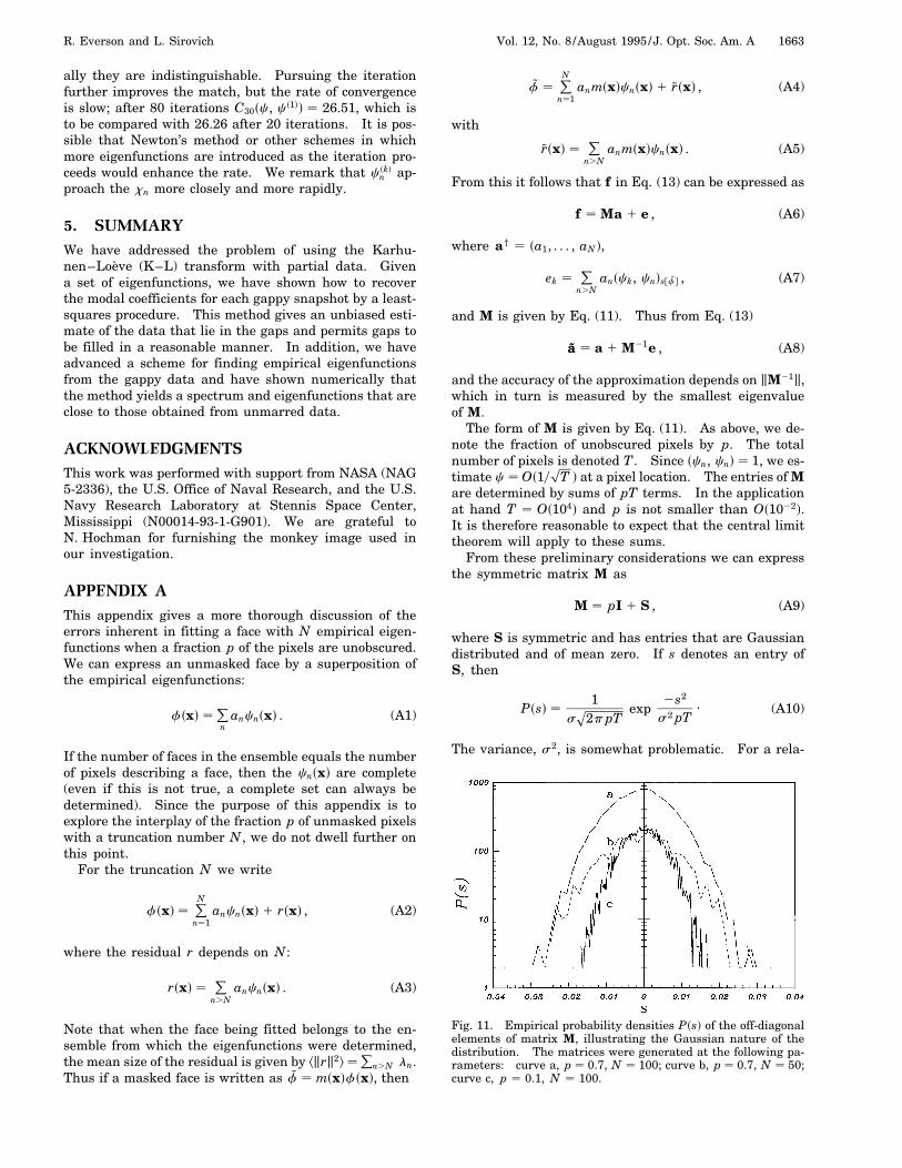
Fig. 11. Empirical probability densities P ssd of the off-diagonalelements of matrix M, illustrating the Gaussian nature of thedistribution. The matrices were generated at the following pa-rameters: curve a, p 0.7, N 100; curve b, p 0.7, N 50;curve c, p 0.1, N 100.


Table 1. Ratio of the Mean Size of the DiagonalElements to the Off-Diagonal Elements of

Matrix M, Divided byp

pTp

pTp

pT , for VariousValues of p and N . Except When p øøø 1, the

Estimate That the Ratio Is Osp

pT dsp

pT dsp

pT d Is Verified

N p Normalized Ratio

10 0.06 1.47100 0.06 1.14150 0.06 1.13200 0.06 1.12

10 0.25 1.18100 0.25 1.31150 0.25 1.27200 0.25 1.29

10 0.5 2.72100 0.5 1.66150 0.5 1.55200 0.5 1.54

10 0.75 3.01100 0.75 2.11150 0.75 2.20200 0.75 2.16

10 0.95 5.28100 0.95 4.98150 0.95 4.59200 0.95 5.05

tively large index, cnsxd is locally sinusoidal. If we adoptthis as a hypothesis, it then follows that s2 Os1yT 2d,and Eq. (A10) takes the form

P ssd p

Ty2pp exps2s2Typd . (A11)

This implies that the off-diagonal terms of M are Osp

pyT dand hence that the ratio of off-diagonal to on-diagonalterms is Os1y

ppyT d. A series of numerical experiments

confirms the Gaussian nature of the entries of S and alsothat the estimate for the ratio is sound (see Fig. 11 andTable 1).

According to Wigner’s semicircle theorem,12,13 a sym-metric random matrix of order N whose entries have zeromean and variance s2 has the eigenvalue density

rsld 1

2pNs2

p4Nl2 2 m2 . (A12)

The theorem applies to S, and since eigenvalues of M arep plus the eigenvalues of S, it follows that the eigenvaluesof M are such that

p 2 2p

pNyT , m , p 1 2p

pNyT . (A13)

If we take the vanishing of the smallest eigenvalue of Mas a criterion for the breakdown of the scheme, then thisoccurs for

N pTy4 . (A14)

In Figs. 3 and 4 we display the errors incurred for variousp for the cases of faces that do not belong to the originalensemble and that do belong to the ensemble that deter-mined the eigenfunctions cn. Given the rough nature ofthe estimate, criterion (A14) is not bad. The two casesdiffer as a result of the fact that kkrk2l is significantlysmaller when the faces belong to the ensemble that de-termines the cn.

REFERENCES1. R. M. Everson, P. Cornillion, L. Sirovich, and A. Webber,

“An empirical eigenfunction analysis of sea surface temper-atures in the Western North Atlantic,” submitted to J. Phys.Oceanogr.

2. L. Sirovich and M. Kirby, “Low-dimensional procedure forthe characterization of human faces,” J. Opt. Soc. Am. A 4,519–524 (1987).

3. M. Kirby and L. Sirovich, “Applications of the Karhunen–Loeve procedure for the characterization of human faces,”IEEE Trans. Pattern Anal. Mach. Intell. 12,103–108 (1990).

4. E. Schmidt, “Zur Theorie der linearen und nichtlinearenIntegralgleichungen. i Teil: Entwicklung willk ulicherFunktion nach Systemen vorgeschriebener,” Math. Annal.63, 433–476 (1907).

5. L. Sirovich and R. M. Everson, “Analysis and managementof large scientific databases,” Int. J. Supercomput. Applic. 6,50–68 (1992).

6. G. W. Stewart, “On the early history of the singular valuedecomposition,” SIAM Rev. 35, 551–566 (1993).

7. G. Berkooz, P. Holmes, and J. L. Lumley, “The proper or-thogonal decomposition in the analysis of turbulent flows,”Ann. Rev. Fluid Mech. 25, 539–575 (1993).

8. M. Turk and A. Pentland, “Eigenfaces for recognition,”J. Cogn. Neurosci. 3, 71–86 (1991).

9. A. J. O’Toole, H. Abdi, K. A. Deffenbacher, and J. C. Bartlett,“Classifying faces by race and sex using an autoassociativememory trained for recognition,” in Proceedings of the Thir-teenth Annual Conference of the Cognitive Science Society,K. J. Hammond and D. Gentner, eds. (Erlbaum, Hillsdale,N.J., 1991), pp. 847–851.

10. A. J. O’Toole, K. A. Deffenbacher, H. Abdi, and J. C. Bartlett,“Simulating the ‘other-race effect’ as a problem in perceptuallearning,” Connection Sci. 3, 163–178 (1991).

11. K. A. Kelly, “The influence of winds and topography on seasurface temperature patterns over the northern Californiaslope,” J. Geophys. Res. 90, 11,783–11,798 (1985).

12. E. P. Wigner, “Random matrices in physics,” SIAM Rev. 9,1–23 (1967).

13. M. Carmeli, Statistical Theory and Random Matrices(Dekker, New York, 1983).

karhunen-loeve procedure for gappy data · r. everson and l. sirovich vol. 12, no. 8/august 1995/j....

Documents