kaplan-meier curves (logrank tests) - · pdf filekaplan-meier curves (logrank tests)...
TRANSCRIPT
NCSS Statistical Software NCSS.com
555-1 © NCSS, LLC. All Rights Reserved.
Chapter 555
Kaplan-Meier Curves (Logrank Tests) Introduction This procedure computes the nonparametric Kaplan-Meier and Nelson-Aalen estimates of survival and associated hazard rates. It can fit complete, right censored, left censored, interval censored (readout), and grouped data values. It outputs various statistics and graphs that are useful in reliability and survival analysis.
It also performs several logrank tests and provides both the parametric and randomization test significance levels.
Overview of Survival Analysis We will give a brief introduction to the subject in this section. For a complete account of survival analysis, we suggest the book by Klein and Moeschberger (1997).
Survival analysis is the study of the distribution of life times. That is, it is the study of the elapsed time between an initiating event (birth, start of treatment, diagnosis, or start of operation) and a terminal event (death, relapse, cure, or machine failure). The data values are a mixture of complete (terminal event occurred) and censored (terminal event has not occurred) observations. From the data values, the survival analyst makes statements about the survival distribution of the failure times. This distribution allows questions about such quantities as survivability, expected life time, and mean time to failure to be answered.
Let T be the elapsed time until the occurrence of a specified event. The event may be death, occurrence of a disease, disappearance of a disease, appearance of a tumor, etc. The probability distribution of T may be specified using one of the following basic functions. Once one of these functions has been specified, the others may be derived using the mathematical relationships presented.
1. Probability density function, f(t). This is the probability that an event occurs at time t.
2. Cumulative distribution function, F(t). This is the probability that an individual survives until time t.
F t f x dxt
( ) ( )= ∫0
3. Survival function, S(T). This is the probability that an individual survives beyond time T. This is usually the primary quantity of interest. It is estimated using the nonparametric Kaplan-Meier curve.
S T f x dx
F TT
( ) ( )
( )
=
= −
∞
∫1
NCSS Statistical Software NCSS.com Kaplan-Meier Curves (Logrank Tests)
555-2 © NCSS, LLC. All Rights Reserved.
( )[ ]
S T h x dx
H T
T
( ) exp ( )
exp
= −
= −
∫0
4. Hazard rate, h(T). This is the probability that an individual at time T experiences the event in the next instant. It is a fundamental quantity in survival analysis. It is also known as the conditional failure rate in reliability, the force of mortality in demography, the intensity function in stochastic processes, the age-specific failure rate in epidemiology, and the inverse of Mill’s ratio in economics. The empirical hazard rate may be used to identify the appropriate probability distribution of a particular mechanism, since each distribution has a different hazard rate function. Some distributions have a hazard rate that decreases with time, others have a hazard rate that increases with time, some are constant, and some exhibit all three behaviors at different points in time.
h T f TS T
( ) ( )( )
=
5. Cumulative hazard function, H(T). This is integral of h(T) from 0 to T.
( )[ ]
H T h x dx
S T
T
( ) ( )
ln
=
= −
∫0
Nonparametric Estimators of Hazard and Survival All of the following results are from Klein and Moeschberger (1997).
The recommended nonparametric estimator of the survival distribution, S(T), is the Kaplan-Meier product-limit estimator. The recommended nonparametric estimator of the cumulative hazard function, H(T), is the Nelson-Aalen estimator. Although each of these estimators could be used to estimate the other quantity using the relationship
( )[ ]H T S T( ) ln= −
or
( ) ( )[ ]S T H T= −exp
this is not recommended.
The following notation will be used to define both of these estimators. Let t M= 1, , index the M unique termination (failure or death) times T T TM1 2, ,..., . Note that M does not include duplicate times or times at which only censored observations occur. Associated with each of these failure times is an entry time Et at which the subject began to be observed. Usually, these entry times are taken to be zero. If positive entry times are specified, the data are said to have been left truncated. When data are left truncated, it is often necessary to define a minimum time, A, below which failures are not considered. When a positive A is used, the unconditional survival function S(T) is changed to a conditional survival function S(T|T>A).
The set of all failures (deaths) that occur at time Tt is referred to as Dt and the number in this set is given by dt . The risk set at t, Rt , is the set of all individuals that are at risk immediately before time Tt . This set includes all individuals whose entry and termination times include Tt . That is, Rt is made up of all individuals with times such that E T Tj t j< ≤ and A Tt≤ . The number of individuals in the risk set is given by rt .
NCSS Statistical Software NCSS.com Kaplan-Meier Curves (Logrank Tests)
555-3 © NCSS, LLC. All Rights Reserved.
Kaplan-Meier Product-Limit Estimator Using the above notation, the Kaplan-Meier product-limit estimator is defined as follows in the range of time values for which there are data.
( )min
minS T
if T Tdr
if T Ti
iA T Ti
=>
−
≤
≤ ≤∏
1
1
The variance of S(T) is estimated by Greenwood’s formula
[ ] ( ) ( )( )
V S T S T dr r d
i
i i iA T Ti
=−≤ ≤
∑2
Pointwise Confidence Intervals of Survival A pointwise confidence interval for the survival probability at a specific time T0 of ( )S T0 is represented by two confidence limits which have been constructed so that the probability that the true survival probability lies between them is 1− α . Note that these limits are constructed for a single time point. Several of them cannot be used together to form a confidence band such that the entire survival function lies within the band. When these are plotted with the survival curve, these limits must be interpreted on an individual, point by point, basis.
Three difference confidence intervals are available. All three confidence intervals perform about the same in large samples. The linear (Greenwood) interval is the most commonly used. However, the log-transformed and the arcsine-square intervals behave better in small to moderate samples, so they are recommended.
Linear (Greenwood) Pointwise Confidence Interval for S(T) This estimator may be used to create a confidence interval at a specific time point T0 of ( )S T0 using the formula
( ) ( )/S T z TS0 1 2 0± −α σ
where
[ ]σ S T
V S T
S T2
00
20
( ) ( ) ( )
=
and z is the appropriate value from the standard normal distribution.
Log-Transformed Pointwise Confidence Interval for S(T) Better confidence limits may be calculated using the logarithmic transformation of the hazard functions. These limits are
( ) , ( )/S T S T01
0θ θ
where
θ σα=
−exp ( )log[ ( )]
/z TS T
S1 2 0
0
NCSS Statistical Software NCSS.com Kaplan-Meier Curves (Logrank Tests)
555-4 © NCSS, LLC. All Rights Reserved.
ArcSine-Square Root Pointwise Confidence Interval for S(T) Another set of confidence limits using an improving transformation is given by the formula
{ }
{ }
sin max ,arcsin ( ) . ( )( )( )
( )
sin min ,arcsin ( ) . ( )( )( )
/
/
/
/
/
/
20
1 2
1 2 00
0
1 2
0
20
1 2
1 2 00
0
1 2
0 0 51
20 5
1
S T z T S TS T
S T
S T z T S TS T
S
S
−−
≤ ≤
+−
−
−
α
α
σ
π σ
Nelson-Aalen Hazard Estimator The Nelson-Aalen estimator is recommended as the best estimator of the cumulative hazard function, H(T). This estimator is give as
~( )min
minH T
if T Tdr
if T Ti
iA T Ti
=>
≤
≤ ≤∑
0
Three estimators of the variance of this estimate are mentioned on page 34 of Therneau and Grambsch (2000). These estimators differ in the way they model tied event times. When there are no event time ties, they give almost identical results.
1. Simple (Poisson) Variance Estimate This estimate assumes that event time ties occur because of rounding and a lack of measurement precision. This estimate is the largest of the three, so it gives the widest, most conservative, confidence limits. The formula for this estimator, derived assuming a Poisson model for the number of deaths, is
σ ~ ( )Hi
iA T T
T dr
i
12
2=≤ ≤∑
2. Plug-in Variance Estimate This estimate also assumes that event time ties occur because of rounding and a lack of measurement precision. The formula for this estimator, derived by substituting sample quantities in the theoretical variance formula, is
( )σ ~ ( )Hi i i
iA T T
Td r d
ri
22
3=−
≤ ≤∑
Note that when ri = 1, a ‘1’ is substituted for ( )r d ri i i− / in this formula.
3. Binomial Variance Estimate This estimate assumes that event time ties occur because the process is fundamentally discrete rather than due to lack of precision and/or rounding. The formula for this estimator, derived assuming a binomial model for the number of events, is
( )( )
σ ~ ( )Hi i i
i iA T T
Td r dr r
i
32
2 1=
−−≤ ≤
∑
Note that when ri = 1, a ‘1’ is substituted for ( ) ( )r d ri i i− −/ 1 in this formula.
NCSS Statistical Software NCSS.com Kaplan-Meier Curves (Logrank Tests)
555-5 © NCSS, LLC. All Rights Reserved.
Which Variance Estimate to Use Therneau and Grambsch (2000) indicate that, as of the writing of their book, there is no clear-cut champion. The simple estimate is often suggested because it is always largest and thus gives the widest, most conservative confidence, confidence limits. In practice, there is little difference between them and the choice of which to use will make little difference in the final interpretation of the data. We have included all three since each occurs alone in various treatises on survival analysis.
Pointwise Confidence Intervals of Cumulative Hazard A pointwise confidence interval for the cumulative hazard at a specific time T0 of ( )H T0 is represented by two confidence limits which have been constructed so that the probability that the true hazard lies between them is
α−1 . Note that these limits are constructed for a single time point. Several of them cannot be used together to form a confidence band such that the entire hazard function lies within the band. When these are plotted with the hazard curve, these limits must be interpreted on an individual, point by point, basis.
Three difference confidence intervals are available. All three confidence intervals perform about the same in large samples. The linear (Greenwood) interval is the most commonly used. However, the log-transformed and the arcsine-square intervals behave better in small to moderate samples, so they are recommended.
Linear Pointwise Confidence Interval for H(T) This estimator may be used to create a confidence interval at a specific time point T0 of ( )H T0 using the formula
~( ) ( )/ ~H T z TH0 1 2 0± −α σ
where z is the appropriate value from the standard normal distribution.
Log-Transformed Pointwise Confidence Interval for H(T) Better confidence limits may be calculated using the logarithmic transformation of the hazard functions. These limits are
~( ) / , ~( )H T H T0 0φ φ
where
( )φ
σα=
−exp
( )~/
~z TH T
H1 2 0
0
ArcSine-Square Root Pointwise Confidence Interval for H(T) Another set of confidence limits using an improving transformation is given by the formula
( ) ( )( ){ }
( ) ( )( ){ }
− −
+
−
≤ ≤
− −
−
−
−
−
22 2 2 1
2 02 2 1
0 1 2 0
0
0
0 1 2 0
0
ln sin min ,arcsin exp~
exp ~
( )
ln sin max ,arcsin exp~
exp ~
/ ~
/ ~
π σ
σ
α
α
H T z T
H T
H T
H T z T
H T
H
H
NCSS Statistical Software NCSS.com Kaplan-Meier Curves (Logrank Tests)
555-6 © NCSS, LLC. All Rights Reserved.
Survival Quantiles The median survival time is an example of a quantile of the survival distribution. It is the smallest value of T such that ( ) .S T = 0 50 . In fact, more general results are available for any quantile p. The pth quantile is estimated by
( ){ }T T S T pp = ≤ −inf : 1
In words, Tp is smallest time at which ( )S T is less than or equal to 1 - p.
A ( )%1100 α− confidence interval for Tp can be generated using each of the three estimation methods. These are given next.
Linear Pointwise Confidence Interval for Tp This confidence interval is given by the set of all times such that
( )( )[ ]
− ≤− −
≤− −zS T p
V S Tz1 2 1 2
1α α/ /
( )
where z is the appropriate value from the standard normal distribution.
Log-Transformed Pointwise Confidence Interval for Tp This confidence interval is given by the set of all times such that
( )[ ]{ } [ ]{ }[ ] [ ][ ]( )[ ]
− ≤− − − −
≤− −zS T p S T S T
V S Tz1 2 1 2
1α α/ /
ln ln ln ln ( )ln ( )
where z is the appropriate value from the standard normal distribution.
ArcSine-Square Root Pointwise Confidence Interval for Tp This confidence interval is given by the set of all times such that
( ) [ ] [ ]( )[ ]
− ≤
− −
−
≤− −zS T p S T S T
V S Tz1 2 1 2
2 1 1α α/ /
arcsin arcsin ( ) ( )
where z is the appropriate value from the standard normal distribution.
Hazard Rate Estimation The characteristics of the failure process are best understood by studying the hazard rate, h(T), which is the derivative (slope) of the cumulative hazard function H(T). The hazard rate is estimated using kernel smoothing of the Nelson-Aalen estimator as given in Klein and Moeschberger (1997). The formulas for the estimated hazard rate and its variance are given by
( )( ) ~h Tb
K T Tb
H Ti
A T Ti
i
=−
≤ ≤
∑1∆
[ ] ( )[ ]σ 22
21( ) ~h Tb
K T Tb
V H Ti
A T Ti
i
=−
≤ ≤
∑ ∆
NCSS Statistical Software NCSS.com Kaplan-Meier Curves (Logrank Tests)
555-7 © NCSS, LLC. All Rights Reserved.
where b is the bandwidth about T and
( ) ( ) ( )∆~ ~ ~H T H T H Tk k k= − −1
( )[ ] ( )[ ] ( )[ ]∆ ~ ~ ~V H T V H T V H Tk k k= − −1
Three choices are available for the kernel function K(x) in the above formulation. These are defined differently for various values of T. Note that the Ti ’s are for failed items only and that TMax is the maximum failure time. For the uniform kernel the formulas for the various values of T are
( )K x for T b T T b= − ≤ ≤ +12
( ) ( )( )
( )( )
K xq
qx for T bL =
+
++
−
+<
4 1
16 11
3
4 3
( ) ( )( )
( )( )
K xr
rr
rx for T b T TR Max Max=
+
+−
−
+− < <
4 1
16 11
3
4 3
where
q Tb
=
and
r T Tb
Max=−
For the Epanechnikov kernel the formulas for the various values of T are
( ) ( )K x x for T b T T b= − − ≤ ≤ +34
1 2
( ) ( )( )K x K x A Bx for T bL = + <
( ) ( )( )K x K x A Bx for T b T TR Max Max= − − − < <
where
( )( ) ( )
Aq q q
q q q=
− + −
+ − +
64 2 4 6 3
1 19 18 3
2 3
4 2
( )( ) ( )
Bq
q q q=
−
+ − +
240 11 19 18 3
2
4 2
q Tb
=
r T Tb
Max=−
NCSS Statistical Software NCSS.com Kaplan-Meier Curves (Logrank Tests)
555-8 © NCSS, LLC. All Rights Reserved.
For the biweight kernel the formulas for the various values of T are
( ) ( )K x x for T b T T b= − − ≤ ≤ +1516
1 2 2
( ) ( )( )K x K x A Bx for T bL = + <
( ) ( )( )K x K x A Bx for T b T TR Max Max= − − − < <
where
( )( ) ( )
Aq q q q
q q q q q=
− + − +
+ − + − +
64 8 24 48 45 15
1 81 168 126 40 5
2 3 4
5 2 3 4
( )( ) ( )
Bq
q q q q q=
−
+ − + − +
1120 11 81 168 126 40 5
3
5 2 3 4
q Tb
=
r T Tb
Max=−
Confidence intervals for h(T) are given by
( )( )[ ]
( ) exp
/h T
z h T
h T±
−1 2α σ
Care must be taken when using this kernel-smoothed estimator since it is actually estimating a smoothed version of the hazard rate, not the hazard rate itself. Thus, it may be biased. Also, it is greatly influenced by the choice of the bandwidth b. We have found that you must experiment with b to find an appropriate value for each dataset.
Hazard Ratio Often, it will be useful to compare the hazard rates of two groups. This is most often accomplished by creating the hazard ratio (HR). The hazard ratio is discussed in depth in Parmar and Machin (1995) and we refer you to this reference for details which we summarize here. The Cox-Mantel estimate of HR for two groups A and B is given by
HR HHO EO E
CMA
B
A A
B B
=
=//
where Oi is the observed number of events (deaths) in group i , Ei is the expected number of events (deaths) in group i, and Hi is the overall hazard rate for the ith group. The calculation of the Ei is explained in Parmar and Machin (1995).
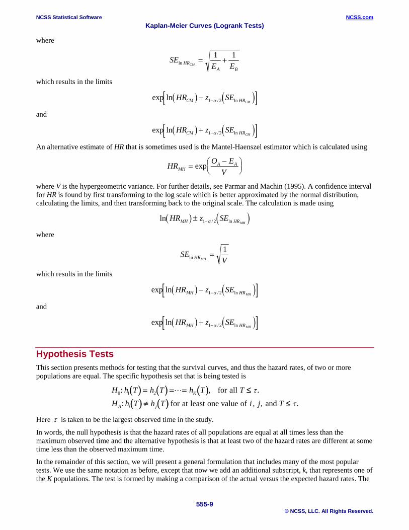
A confidence interval for HR is found by first transforming to the log scale which is better approximated by the normal distribution, calculating the limits, and then transforming back to the original scale. The calculation is made using
( ) ( )ln / lnHR z SECM HRCM± −1 2α
NCSS Statistical Software NCSS.com Kaplan-Meier Curves (Logrank Tests)
555-9 © NCSS, LLC. All Rights Reserved.
where
SEE EHR
A BCMln = +
1 1
which results in the limits
( ) ( )[ ]exp ln / lnHR z SECM HRCM− −1 2α
and
( ) ( )[ ]exp ln / lnHR z SECM HRCM+ −1 2α
An alternative estimate of HR that is sometimes used is the Mantel-Haenszel estimator which is calculated using
HR O EVMH
A A=−
exp
where V is the hypergeometric variance. For further details, see Parmar and Machin (1995). A confidence interval for HR is found by first transforming to the log scale which is better approximated by the normal distribution, calculating the limits, and then transforming back to the original scale. The calculation is made using
( ) ( )ln / lnHR z SEMH HRMH± −1 2α
where
SEVHRMHln =1
which results in the limits
( ) ( )[ ]exp ln / lnHR z SEMH HRMH− −1 2α
and
( ) ( )[ ]exp ln / lnHR z SEMH HRMH+ −1 2α
Hypothesis Tests This section presents methods for testing that the survival curves, and thus the hazard rates, of two or more populations are equal. The specific hypothesis set that is being tested is
( ) ( ) ( )( ) ( )
H h T h T h T T
H h T h T i j TK
A i j
0 1 2: , .
: , .
= = = ≤
≠ ≤
for all
for at least one value of , and
τ
τ
Here τ is taken to be the largest observed time in the study.
In words, the null hypothesis is that the hazard rates of all populations are equal at all times less than the maximum observed time and the alternative hypothesis is that at least two of the hazard rates are different at some time less than the observed maximum time.
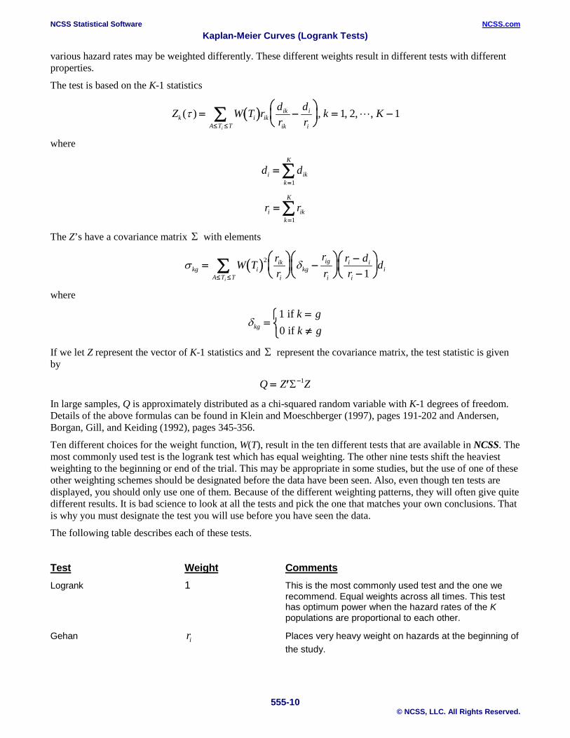
In the remainder of this section, we will present a general formulation that includes many of the most popular tests. We use the same notation as before, except that now we add an additional subscript, k, that represents one of the K populations. The test is formed by making a comparison of the actual versus the expected hazard rates. The
NCSS Statistical Software NCSS.com Kaplan-Meier Curves (Logrank Tests)
555-10 © NCSS, LLC. All Rights Reserved.
various hazard rates may be weighted differently. These different weights result in different tests with different properties.
The test is based on the K-1 statistics
( )Z W T r dr
dr
k Kk i ikik
ik
i
iA T Ti
( ) , , , ,τ = −
= −
≤ ≤∑ 1 2 1
where
d di ikk
K
==∑
1
r ri ikk
K
==∑
1
The Z’s have a covariance matrix Σ with elements
( )σ δkg iik
ikg
ig
i
i i
iA T TiW T r
rrr
r dr
di
=
−
−−
≤ ≤∑ 2
1
where
δkg
k gk g
==≠
1 if 0 if
If we let Z represent the vector of K-1 statistics and Σ represent the covariance matrix, the test statistic is given by
Q Z Z= ′ −Σ 1
In large samples, Q is approximately distributed as a chi-squared random variable with K-1 degrees of freedom. Details of the above formulas can be found in Klein and Moeschberger (1997), pages 191-202 and Andersen, Borgan, Gill, and Keiding (1992), pages 345-356.
Ten different choices for the weight function, W(T), result in the ten different tests that are available in NCSS. The most commonly used test is the logrank test which has equal weighting. The other nine tests shift the heaviest weighting to the beginning or end of the trial. This may be appropriate in some studies, but the use of one of these other weighting schemes should be designated before the data have been seen. Also, even though ten tests are displayed, you should only use one of them. Because of the different weighting patterns, they will often give quite different results. It is bad science to look at all the tests and pick the one that matches your own conclusions. That is why you must designate the test you will use before you have seen the data.
The following table describes each of these tests.
Test Weight Comments Logrank 1 This is the most commonly used test and the one we
recommend. Equal weights across all times. This test has optimum power when the hazard rates of the K populations are proportional to each other.
Gehan ri Places very heavy weight on hazards at the beginning of the study.
NCSS Statistical Software NCSS.com Kaplan-Meier Curves (Logrank Tests)
555-11 © NCSS, LLC. All Rights Reserved.
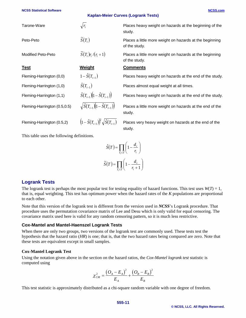
Tarone-Ware ir Places heavy weight on hazards at the beginning of the study.
Peto-Peto ( )iTS~ Places a little more weight on hazards at the beginning of the study.
Modified Peto-Peto ( ) ( )1/~ +iii rrTS Places a little more weight on hazards at the beginning of the study.
Test Weight Comments
Fleming-Harrington (0,0) ( )1ˆ1 −− iTS Places heavy weight on hazards at the end of the study.
Fleming-Harrington (1,0) ( )1ˆ
−iTS Places almost equal weight at all times.
Fleming-Harrington (1,1) ( ) ( )( )11ˆ1ˆ
−− − ii TSTS Places heavy weight on hazards at the end of the study.
Fleming-Harrington (0.5,0.5) ( ) ( )( )11ˆ1ˆ
−− − ii TSTS Places a little more weight on hazards at the end of the study.
Fleming-Harrington (0.5,2) ( )( ) ( )12
1ˆˆ1 −−− ii TSTS Places very heavy weight on hazards at the end of the
study. This table uses the following definitions.
( ) ∏≤
−=
TT i
i
irdTS 1ˆ
( ) ∏≤
+
−=TT i
i
ir
dTS1
1~
Logrank Tests The logrank test is perhaps the most popular test for testing equality of hazard functions. This test uses W(T) = 1, that is, equal weighting. This test has optimum power when the hazard rates of the K populations are proportional to each other.
Note that this version of the logrank test is different from the version used in NCSS’s Logrank procedure. That procedure uses the permutation covariance matrix of Lee and Desu which is only valid for equal censoring. The covariance matrix used here is valid for any random censoring pattern, so it is much less restrictive.
Cox-Mantel and Mantel-Haenszel Logrank Tests When there are only two groups, two versions of the logrank test are commonly used. These tests test the hypothesis that the hazard ratio (HR) is one; that is, that the two hazard rates being compared are zero. Note that these tests are equivalent except in small samples.
Cox-Mantel Logrank Test Using the notation given above in the section on the hazard ratios, the Cox-Mantel logrank test statistic is computed using
( ) ( )χCMA A
A
B B
B
O EE
O EE
22 2
=−
+−
This test statistic is approximately distributed as a chi-square random variable with one degree of freedom.
NCSS Statistical Software NCSS.com Kaplan-Meier Curves (Logrank Tests)
555-12 © NCSS, LLC. All Rights Reserved.
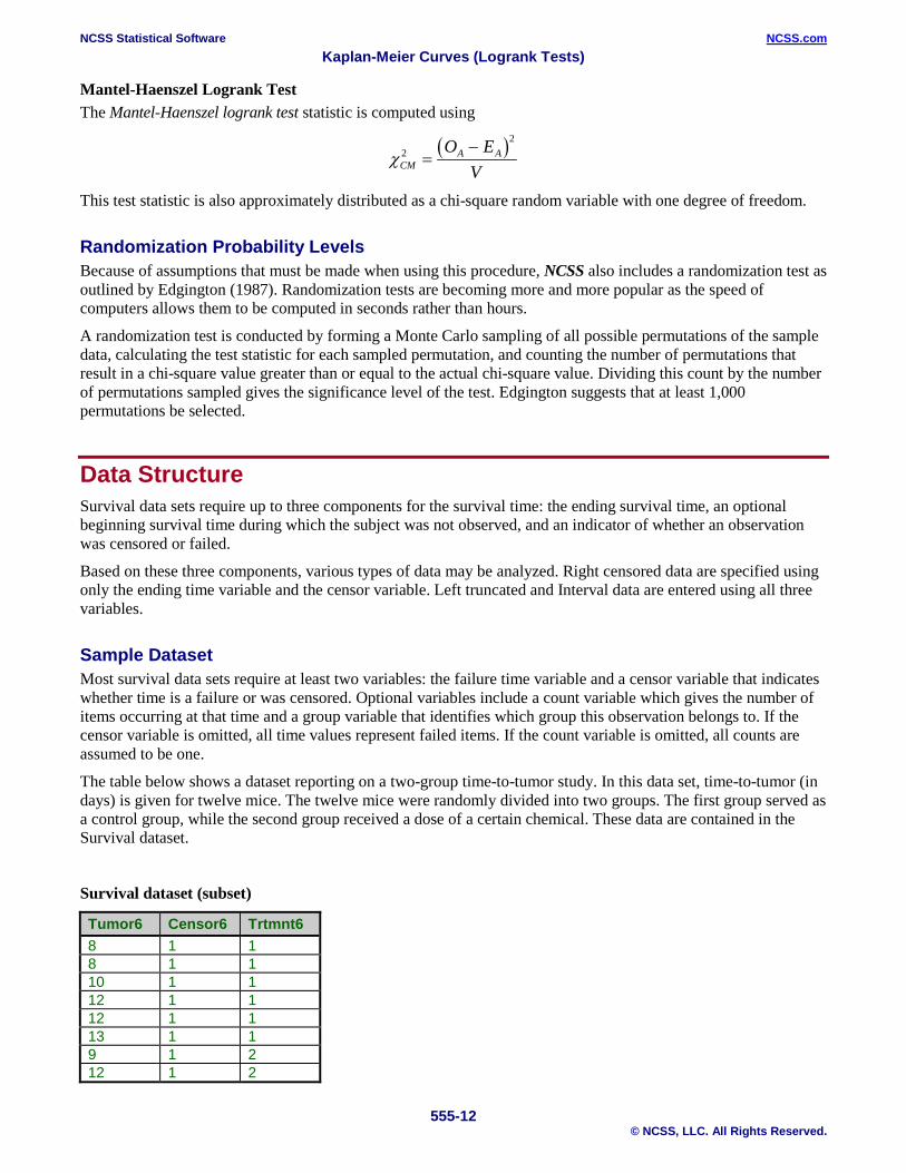
Mantel-Haenszel Logrank Test The Mantel-Haenszel logrank test statistic is computed using
( )χCMA AO E
V2
2
=−
This test statistic is also approximately distributed as a chi-square random variable with one degree of freedom.
Randomization Probability Levels Because of assumptions that must be made when using this procedure, NCSS also includes a randomization test as outlined by Edgington (1987). Randomization tests are becoming more and more popular as the speed of computers allows them to be computed in seconds rather than hours.
A randomization test is conducted by forming a Monte Carlo sampling of all possible permutations of the sample data, calculating the test statistic for each sampled permutation, and counting the number of permutations that result in a chi-square value greater than or equal to the actual chi-square value. Dividing this count by the number of permutations sampled gives the significance level of the test. Edgington suggests that at least 1,000 permutations be selected.
Data Structure Survival data sets require up to three components for the survival time: the ending survival time, an optional beginning survival time during which the subject was not observed, and an indicator of whether an observation was censored or failed.
Based on these three components, various types of data may be analyzed. Right censored data are specified using only the ending time variable and the censor variable. Left truncated and Interval data are entered using all three variables.
Sample Dataset Most survival data sets require at least two variables: the failure time variable and a censor variable that indicates whether time is a failure or was censored. Optional variables include a count variable which gives the number of items occurring at that time and a group variable that identifies which group this observation belongs to. If the censor variable is omitted, all time values represent failed items. If the count variable is omitted, all counts are assumed to be one.
The table below shows a dataset reporting on a two-group time-to-tumor study. In this data set, time-to-tumor (in days) is given for twelve mice. The twelve mice were randomly divided into two groups. The first group served as a control group, while the second group received a dose of a certain chemical. These data are contained in the Survival dataset.
Survival dataset (subset)
Tumor6 Censor6 Trtmnt6 8 1 1 8 1 1 10 1 1 12 1 1 12 1 1 13 1 1 9 1 2 12 1 2
NCSS Statistical Software NCSS.com Kaplan-Meier Curves (Logrank Tests)
555-13 © NCSS, LLC. All Rights Reserved.
Procedure Options This section describes the options available in this procedure.
Variables Tab This panel specifies the variables used in the analysis.
Time Variables
(Elapsed) Time Variable This variable contains the length of time that an individual was observed. This may represent a failure time or a censor time. Whether the subject actually died is specified by the Censor Variable. Since the values are elapsed times, they must be positive. Zeroes and negative values are treated as missing values. During the maximum likelihood calculations, a risk set is defined for each individual. The risk set is defined to be those subjects who were being observed at this subject’s failure and who lived as long or longer. It may take several rows of data to specify a subject’s history. This variable and the Entry Time Variable define a period during which the individual was at risk of failing. If the Entry Time Variable is not specified, its value is assumed to be zero. Several types of data may be entered. These will be explained next.
• Failure This type of data occurs when a subject is followed from their entrance into the study until their death. The failure time is entered in this variable and the Censor Variable is set to the failed code, which is often a one.
The Entry Time Variable is not necessary. If an Entry Time Variable is used, its value should be zero for this type of observation.
• Interval Failure This type of data occurs when a subject is known to have died during a certain interval. The subject may, or may not, have been observed during other intervals. If they were, they are treated as Interval Censored data. An individual may require several rows on the database to record their complete follow-up history.
For example, suppose the condition of the subjects is only available at the end of each month. If a subject fails during the fifth month, two rows of data would be required. One row, representing the failure, would have a Time of 5.0 and an Entry Time of 4.0. The Censor variable would contain the failure code. A second row, representing the prior periods, would have a Time of 4.0 and an Entry Time of 0.0. The Censor variable would contain the censor code.
• Right Censored This type of data occurs when a subject has not failed up to the specified time. For example, suppose that a subject enters the study and does not die until after the study ends 12 months later. The subject’s time (365 days) is entered here. The Censor variable contains the censor code.
• Interval Censored This type of data occurs when a subject is known not to have died during a certain interval. The subject may, or may not, have been observed during other intervals. An individual may require several rows on the database to record their complete follow-up history.

NCSS Statistical Software NCSS.com Kaplan-Meier Curves (Logrank Tests)
555-14 © NCSS, LLC. All Rights Reserved.
For example, suppose the condition of the subjects is only available at the end of each month. If a subject fails during the fifth month, two rows of data would be required. One row, representing the failure, would have a Time of 5.0 and an Entry Time of 4.0. The Censor variable would contain the failure code. A second row, representing the prior periods, would have a Time of 4.0 and an Entry Time of 0.0. The Censor variable would contain the censor code.
Entry Time Variable This optional variable contains the elapsed time before an individual entered the study. Usually, this value is zero. However, in cases such as left truncation and interval censoring, this value defines a time period before which the individual was not observed. Negative entry times are treated as missing values. It is possible for the entry time to be zero.
Min Entry Time When you have left truncation, this value gives the minimum entry time after which events are considered. When used, all survival and hazard rates are conditional on the subject reaching this age.When there is no left truncation (Entry Time Variable), this value is set to zero.
This value is necessary because with left truncation, it is possible for the Kaplan-Meier estimate to reach (and then stay at) zero to soon. Conditioning the probability statements so that this age must be reached in order for an individual to be in a risk set removes this zeroing out problem.
Frequency Variable
Frequency Variable This variable gives the count, or frequency, of the time displayed on that row. When omitted, each row receives a frequency of one. Frequency values should be positive integers. This is usually used to indicate the number of right censored values at the end of a study or the number of failures occurring within an interval. It may also be used to indicate ties for failure data.
Censor Variable
Censor Variable The values in this variable indicate whether the value of the Time Variable represents a censored time or a failure time. These values may be text or numeric. The interpretation of these codes is specified by the Failed and Censored options to the right of this option. Only two values are used, the Failure code and the Censor code. The Unknown Type option specifies what is to be done with values that do not match either the Failure code or the Censor code. Rows with missing values (blanks) in this variable are omitted.
Failed This value identifies those values of the Censor Variable that indicate that the Time Variable gives a failure time. The value may be a number or a letter. We suggest the letter ‘F’ or the number ‘1’ when you are in doubt as to what to use. A failed observation is one in which the time until the event of interest was measured exactly; for example, the subject died of the disease being studied. The exact failure time is known.
(Left Censoring) When the exact failure time is not known, but instead only an upper bound on the failure time is known, the time value is said to have been left censored. In this case, the time value is treated as if it were the true failure time, not just an upper bound. So left censored observations should be coded as failed observations.

NCSS Statistical Software NCSS.com Kaplan-Meier Curves (Logrank Tests)
555-15 © NCSS, LLC. All Rights Reserved.
Censored This value identifies those values of the Censor Variable that indicate that the individual recorded on this row was censored. That is, the actual failure time occurs sometime after the value of the Time Variable. We suggest the letter ‘C’ or the number ‘0’ when you are in doubt as to what to use. A censored observation is one in which the time until the event of interest is not known because the individual withdrew from the study, the study ended before the individual failed, or for some similar reason. Note that it does not matter whether the censoring was Right or Interval. All you need to indicate here is that they were censored.
Unknown Censor This option specifies what the program is to assume about rows whose censor value is not equal to either the Failed code or the Censored code. Note that observations with missing censor values are always treated as missing.
• Censored Observations with unknown censor values are assumed to have been censored.
• Failed Observations with unknown censor values are assumed to have failed.
• Missing Observations with unknown censor values are assumed to be missing and they are removed from the analysis.
Group Variable
Group Variable An optional categorical (grouping) variable may be specified. If it is used, a separate analysis is conducted for each unique value of this variable and the log rank tests are performed. If it is not specified, the log rank tests cannot be generated.
Resampling
Run Randomization tests Check this option to run randomization tests. Note that these tests are computer-intensive and may require a great deal of time to run.
Monte Carlo Samples Specify the number of Monte Carlo samples used when conducting randomization tests. You also need to check the ‘Run randomization tests’ box to run these tests. Somewhere between 1,000 and 100,000 Monte Carlo samples are usually necessary. We suggest the use of 10,000.
Options – KM Survival and Cumulative Hazard
Confidence Limits This option specifies the method used to estimate the confidence limits of the Kaplan-Meier Survival and the Cumulative Hazard. The options are:
• Linear This is the classical method which uses Greenwood’s estimate of the variance.
NCSS Statistical Software NCSS.com Kaplan-Meier Curves (Logrank Tests)
555-16 © NCSS, LLC. All Rights Reserved.
• Log Transform This method uses the logarithmic transformation of Greenwood’s variance estimate. It produces better limits than the Linear method and has better small sample properties.
• ArcSine This method uses the arcsine square-root transformation of Greenwood’s variance estimate to produce better limits.
Variance The option specifies which estimator of the variance of the Nelson-Aalen cumulative hazard estimate is to be used. Three estimators have been proposed. When there are no event-time ties, all three give about the same results.
We recommend that you use the Simple estimator unless ties occur naturally in the theoretical event times.
• Simple This estimator should be used when event-time ties are caused by rounding and lack of measurement precision. This estimate gives the largest value and hence the widest, most conservation, confidence intervals.
• Plug In This estimator should be used when event-time ties are caused by rounding and lack of measurement precision.
• Binomial This estimator should be used when ties occur in the theoretical distribution of event times.
Options – Hazard Rate The following options control the calculation of the hazard rate and cumulative hazard function.
Bandwidth Method This option designates the method used to specify the smoothing bandwidth used to calculate the hazard rate. Specify an amount or a percentage of the time range. The default is to specify a percent of the time range.
Bandwidth Amount This option specifies the bandwidth size used to calculate the hazard rate. If the Bandwidth Method was set to Amount, this is a value in time units (such as 10 hours). If Percentage of Time Range was selected, this is a percentage of the overall range of the data.
Smoothing Kernel This option specifies the kernel function used in the smoothing to estimate the hazard rate. You can select uniform, Epanechnikov, or biweight smoothing. The actual formulas for these functions were provided above.
Reports Tab The following options control which reports are displayed and the format of those reports.
Select Reports
Data Summary Section - Hazard Ratio Tests These options indicate whether to display the corresponding report.
NCSS Statistical Software NCSS.com Kaplan-Meier Curves (Logrank Tests)
555-17 © NCSS, LLC. All Rights Reserved.
Alpha Level This is the value of alpha used in the calculation of confidence limits. For example, if you specify 0.04 here, then 96% confidence limits will be calculated.
Report Options
Precision Specify the precision of numbers in the report. A single-precision number will show seven-place accuracy, while a double-precision number will show thirteen-place accuracy. Note that the reports are formatted for single precision. If you select double precision, some numbers may run into others. Also note that all calculations are performed in double precision regardless of which option you select here. Single precision is for reporting purposes only.
Variable Names This option lets you select whether to display only variable names, variable labels, or both.
Value Labels This option lets you select whether to display only values, only value labels, or both for values of the group variable. Use this option if you want to automatically attach labels to the values of the group variable (like 1=Male, 2=Female, etc.). See the section on specifying Value Labels elsewhere in this manual.
Report Options – Survival and Hazard Rate Calculation Values
Percentiles This option specifies a list of percentiles (range 1 to 99) at which the reliability (survivorship) is reported. The values should be separated by commas. You can specify sequences with a colon, putting the increment inside parentheses after the maximum in the sequence. For example: 5:25(5) means 5,10,15,20,25 and 1:5(2),10:20(2) means 1,3,5,10,12,14,16,18,20.
Times This option specifies a list of times at which the percent surviving and cumulative hazard values are reported. Individual values are separated by commas. You can specify a sequence by specifying the minimum and maximum separate by a colon and putting the increment inside parentheses. For example: 5:25(5) means 5,10,15,20,25. Avoid 0 and negative numbers. Use ‘(10)’ alone to specify ten values between zero and the maximum value found in the data.
Report Options – Decimal Places
Time This option specifies the number of decimal places shown on reported time values.
Probability This option specifies the number of decimal places shown on reported probability and hazard values.
Chi-Square This option specifies the number of decimal places shown on reported chi-square values.
Ratio This option specifies the number of decimal places shown on reported ratio values.

NCSS Statistical Software NCSS.com Kaplan-Meier Curves (Logrank Tests)
555-18 © NCSS, LLC. All Rights Reserved.
Plots Tab The following options control the plots that are displayed.
Select Plots These options specify which plots type of plots are displayed.
Survival/Reliability Plot – Hazard Rate Plot Specify whether to display each of these plots. Click the plot format button to change the plot settings.
Plot Options – Plot Contents These options control objects that are displayed on all plots.
Function Line Indicate whether to display the estimated survival (Kaplan-Meier) or hazard function on the plots.
C.L. Lines Indicate whether to display the confidence limits of the estimated function on the plots.
Select Plots – Plots Displayed
Individual-Group Plots When checked, this option specifies that a separate chart of each designated type is displayed.
Combined Plots When checked, this option specifies that a chart combining all groups is to be displayed.
Plot Options – Plot Arrangement These options control the size and arrangement of the plots.
Two Plots Per Line When a man charts are specified, checking this option will cause the size of the charts to be reduced so that they can be displayed two per line. This will reduce the overall size of the output.
Storage Tab These options let you specify if, and where on the dataset, various statistics are stored.
Warning: Any data already in these columns are replaced by the new data. Be careful not to specify columns that contain important data.
Data Storage Options
Storage Option This option controls whether the values indicated below are stored on the dataset when the procedure is run.
• Do not store data No data are stored even if they are checked.
NCSS Statistical Software NCSS.com Kaplan-Meier Curves (Logrank Tests)
555-19 © NCSS, LLC. All Rights Reserved.
• Store in empty columns only The values are stored in empty columns only. Columns containing data are not used for data storage, so no data can be lost.
• Store in designated columns Beginning at the First Storage Variable, the values are stored in this column and those to the right. If a column contains data, the data are replaced by the storage values. Care must be used with this option because it cannot be undone.
Store First Item In The first item is stored in this column. Each additional item that is checked is stored in the columns immediately to the right of this column.
Leave this value blank if you want the data storage to begin in the first blank column on the right-hand side of the data.
Warning: any existing data in these columns is automatically replaced.
Data Storage Options – Select Items to Store with the Dataset
Survival Group - Hazard Rate UCL Indicate whether to store these values, beginning at the column indicated by the Store First Item In option.

NCSS Statistical Software NCSS.com Kaplan-Meier Curves (Logrank Tests)
555-20 © NCSS, LLC. All Rights Reserved.
Example 1 – Kaplan-Meier Survival Analysis This section presents an example of how to analyze a typical set of survival data. In this study, thirty subjects were watched to see how long until a certain event happened after the subject received a certain treatment. The study was terminated at 152.7 hours. At this time, the event had not occurred in eighteen of the subjects. The data used are recorded in the Weibull dataset. You may follow along here by making the appropriate entries or load the completed template Example 1 by clicking on Open Example Template from the File menu of the Kaplan-Meier Curves (Logrank Tests) Fitting window.
1 Open the Weibull dataset. • From the File menu of the NCSS Data window, select Open Example Data. • Click on the file Weibull.NCSS. • Click Open.
2 Open the Kaplan-Meier Curves (Logrank Tests) window. • Using the Analysis menu or the Procedure Navigator, find and select the Kaplan-Meier Curves
(Logrank Tests) procedure. • On the menus, select File, then New Template. This will fill the procedure with the default template.
3 Specify the variables. • On the Kaplan-Meier Curves (Logrank Tests) window, select the Variables tab. • Set the Time Variable to Time. • Set the Censor Variable to Censor. • Set the Frequency Variable to Count.
4 Specify the reports. • Select the Reports tab. • Set the Times box to 10:150(10).
5 Specify the plots. • Select the Plots tab. • Check Hazard Function Plot. • Check Hazard Rate Plot. • Check C.L. Lines by clicking the format button and checking the Confidence Limits box.
6 Run the procedure. • From the Run menu, select Run Procedure. Alternatively, just click the green Run button.
Data Summary Section Data Summary Section Type of Observation Rows Count Minimum Maximum Failed 12 12 12.5 152.7 Censored 1 18 152.7 152.7 Total 13 30 12.5 152.7
This report displays a summary of the amount of data that were analyzed. Scan this report to determine if there were any obvious data errors by double checking the counts and the minimum and maximum times.
NCSS Statistical Software NCSS.com Kaplan-Meier Curves (Logrank Tests)
555-21 © NCSS, LLC. All Rights Reserved.
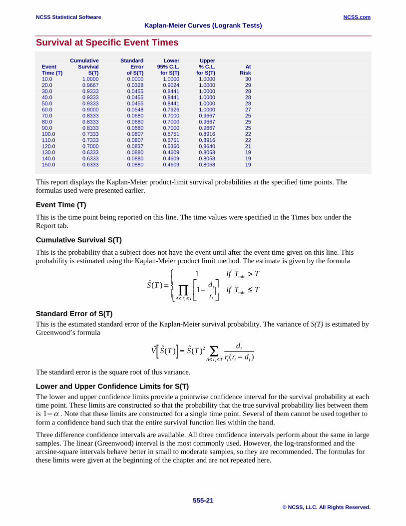
Survival at Specific Event Times
Cumulative Standard Lower Upper Event Survival Error 95% C.L. % C.L. At Time (T) S(T) of S(T) for S(T) for S(T) Risk 10.0 1.0000 0.0000 1.0000 1.0000 30 20.0 0.9667 0.0328 0.9024 1.0000 29 30.0 0.9333 0.0455 0.8441 1.0000 28 40.0 0.9333 0.0455 0.8441 1.0000 28 50.0 0.9333 0.0455 0.8441 1.0000 28 60.0 0.9000 0.0548 0.7926 1.0000 27 70.0 0.8333 0.0680 0.7000 0.9667 25 80.0 0.8333 0.0680 0.7000 0.9667 25 90.0 0.8333 0.0680 0.7000 0.9667 25 100.0 0.7333 0.0807 0.5751 0.8916 22 110.0 0.7333 0.0807 0.5751 0.8916 22 120.0 0.7000 0.0837 0.5360 0.8640 21 130.0 0.6333 0.0880 0.4609 0.8058 19 140.0 0.6333 0.0880 0.4609 0.8058 19 150.0 0.6333 0.0880 0.4609 0.8058 19
This report displays the Kaplan-Meier product-limit survival probabilities at the specified time points. The formulas used were presented earlier.
Event Time (T) This is the time point being reported on this line. The time values were specified in the Times box under the Report tab.
Cumulative Survival S(T) This is the probability that a subject does not have the event until after the event time given on this line. This probability is estimated using the Kaplan-Meier product limit method. The estimate is given by the formula
( )min
minS T
if T Tdr
if T Ti
iA T Ti
=>
−
≤
≤ ≤∏
1
1
Standard Error of S(T) This is the estimated standard error of the Kaplan-Meier survival probability. The variance of S(T) is estimated by Greenwood’s formula
[ ] ( ) ( )( )
V S T S T dr r d
i
i i iA T Ti
=−≤ ≤
∑2
The standard error is the square root of this variance.
Lower and Upper Confidence Limits for S(T) The lower and upper confidence limits provide a pointwise confidence interval for the survival probability at each time point. These limits are constructed so that the probability that the true survival probability lies between them is 1− α . Note that these limits are constructed for a single time point. Several of them cannot be used together to form a confidence band such that the entire survival function lies within the band.
Three difference confidence intervals are available. All three confidence intervals perform about the same in large samples. The linear (Greenwood) interval is the most commonly used. However, the log-transformed and the arcsine-square intervals behave better in small to moderate samples, so they are recommended. The formulas for these limits were given at the beginning of the chapter and are not repeated here.

NCSS Statistical Software NCSS.com Kaplan-Meier Curves (Logrank Tests)
555-22 © NCSS, LLC. All Rights Reserved.
At Risk This value is the number of individuals at risk. The number at risk is all those under study who died or were censored at a time later than the current time. As the number of individuals at risk is decreased, the estimates become less reliable.
Quantiles of Survival Time
Lower Upper 95% C.L. 95% C.L. Proportion Proportion Survival Survival Survival Surviving Failing Time Time Time 0.9500 0.0500 24.4 12.5 69.1 0.9000 0.1000 58.2 24.4 96.6 0.8500 0.1500 69.1 24.4 114.2 0.8000 0.2000 95.5 58.2 125.6 0.7500 0.2500 97.0 68.0 152.7 0.7000 0.3000 114.2 69.1 152.7 0.6500 0.3500 125.6 96.6 152.7 0.6000 0.4000 152.7 97.0 152.7 0.5500 0.4500 114.2 152.7 0.5000 0.5000 123.2 152.7 0.4500 0.5500 152.7 152.7 0.4000 0.6000 152.7 0.3500 0.6500 152.7 0.3000 0.7000 152.7 0.2500 0.7500 152.7 0.2000 0.8000 152.7 0.1500 0.8500 152.7 0.1000 0.9000 152.7 0.0500 0.9500 152.7
This report displays the estimated survival times for various survival proportions. For example, it gives the median survival time if it can be estimated.
Proportion Surviving This is the proportion surviving that is reported on this line. The proportion values were specified in the Percentiles box under the Report tab.
Proportion Failing This is the proportion failing. The proportion is equal to one minus the proportion surviving.
Survival Time This is the time value corresponding to the proportion surviving. The pth quantile is estimated by
( ){ }T T S T pp = ≤ −inf : 1
In words, Tp is smallest time at which ( )S T is less than or equal to 1 - p.
For example, this table estimates that 95% of the subjects will survive longer than 24.4 hours.
Lower and Upper Confidence Limits on Survival Time
These values provide a pointwise ( )%1100 α− confidence interval for Tp . For example, if p is 0.50, this provides a confidence interval for the median survival time.
Three methods are available for calculating these confidence limits. The method is designated under the Variables tab in the Confidence Limits box. The formulas for these confidence limits were given in the Survival Quantiles section.
NCSS Statistical Software NCSS.com Kaplan-Meier Curves (Logrank Tests)
555-23 © NCSS, LLC. All Rights Reserved.
Note that because of censoring, estimates and confidence limits are not available for all survival proportions.
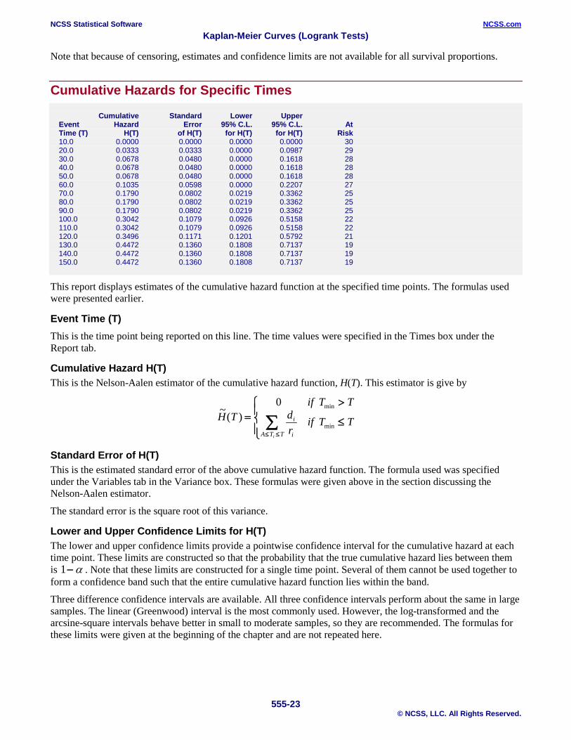
Cumulative Hazards for Specific Times
Cumulative Standard Lower Upper Event Hazard Error 95% C.L. 95% C.L. At Time (T) H(T) of H(T) for H(T) for H(T) Risk 10.0 0.0000 0.0000 0.0000 0.0000 30 20.0 0.0333 0.0333 0.0000 0.0987 29 30.0 0.0678 0.0480 0.0000 0.1618 28 40.0 0.0678 0.0480 0.0000 0.1618 28 50.0 0.0678 0.0480 0.0000 0.1618 28 60.0 0.1035 0.0598 0.0000 0.2207 27 70.0 0.1790 0.0802 0.0219 0.3362 25 80.0 0.1790 0.0802 0.0219 0.3362 25 90.0 0.1790 0.0802 0.0219 0.3362 25 100.0 0.3042 0.1079 0.0926 0.5158 22 110.0 0.3042 0.1079 0.0926 0.5158 22 120.0 0.3496 0.1171 0.1201 0.5792 21 130.0 0.4472 0.1360 0.1808 0.7137 19 140.0 0.4472 0.1360 0.1808 0.7137 19 150.0 0.4472 0.1360 0.1808 0.7137 19
This report displays estimates of the cumulative hazard function at the specified time points. The formulas used were presented earlier.
Event Time (T) This is the time point being reported on this line. The time values were specified in the Times box under the Report tab.
Cumulative Hazard H(T) This is the Nelson-Aalen estimator of the cumulative hazard function, H(T). This estimator is give by
~( )min
minH T
if T Tdr
if T Ti
iA T Ti
=>
≤
≤ ≤∑
0
Standard Error of H(T) This is the estimated standard error of the above cumulative hazard function. The formula used was specified under the Variables tab in the Variance box. These formulas were given above in the section discussing the Nelson-Aalen estimator.
The standard error is the square root of this variance.
Lower and Upper Confidence Limits for H(T) The lower and upper confidence limits provide a pointwise confidence interval for the cumulative hazard at each time point. These limits are constructed so that the probability that the true cumulative hazard lies between them is 1− α . Note that these limits are constructed for a single time point. Several of them cannot be used together to form a confidence band such that the entire cumulative hazard function lies within the band.
Three difference confidence intervals are available. All three confidence intervals perform about the same in large samples. The linear (Greenwood) interval is the most commonly used. However, the log-transformed and the arcsine-square intervals behave better in small to moderate samples, so they are recommended. The formulas for these limits were given at the beginning of the chapter and are not repeated here.

NCSS Statistical Software NCSS.com Kaplan-Meier Curves (Logrank Tests)
555-24 © NCSS, LLC. All Rights Reserved.
At Risk This value is the number of individuals at risk. The number at risk is all those under study who died or were censored at a time later than the current time. As the number of individuals at risk is decreased, the estimates become less reliable.
Hazard Rates Section
95% Lower 95% Upper Nonparametric Std Error of Conf. Limit of Conf. Limit of Failure Hazard Hazard Hazard Hazard Time Rate Rate Rate Rate 10.0 0.0018 0.0014 0.0004 0.0085 20.0 0.0018 0.0013 0.0005 0.0073 30.0 0.0015 0.0010 0.0004 0.0055 40.0 0.0016 0.0009 0.0005 0.0047 50.0 0.0022 0.0012 0.0008 0.0063 60.0 0.0026 0.0015 0.0008 0.0080 70.0 0.0034 0.0016 0.0014 0.0084 80.0 0.0042 0.0017 0.0019 0.0095 90.0 0.0043 0.0019 0.0018 0.0101 100.0 0.0048 0.0021 0.0020 0.0111 110.0 0.0054 0.0022 0.0024 0.0121 120.0 0.0047 0.0021 0.0019 0.0113 130.0 0.0038 0.0020 0.0014 0.0105 140.0 0.0036 0.0025 0.0009 0.0143 150.0 0.0066 0.0066 0.0009 0.0468
This report displays estimates of the hazard rates at the specified time points. The formulas used were presented earlier.
Failure Time This is the time point being reported on this line. The time values were specified in the Times box under the Report tab.
Nonparametric Hazard Rate The characteristics of the failure process are best understood by studying the hazard rate, h(T), which is the derivative (slope) of the cumulative hazard function H(T). The hazard rate is estimated using kernel smoothing of the Nelson-Aalen estimator as given in Klein and Moeschberger (1997). The formulas used were given earlier and are not repeated here.
Care must be taken when using this kernel-smoothed estimator since it is actually estimating a smoothed version of the hazard rate, not the hazard rate itself. Thus, it may be biased. Also, it is greatly influenced by the choice of the bandwidth b. We have found that you must experiment with b to find an appropriate value for each dataset.
The values of the smoothing parameters are specified under the Hazards tab.
Standard Error of Hazard Rate This is the estimated standard error of the above hazard rate. The formula used was specified under the Variables tab in the Variance box. These formulas were given above in the section discussing the Nelson-Aalen estimator.
The standard error is the square root of this variance.
Lower and Upper Confidence Limits of Hazard Rate The lower and upper confidence limits provide a pointwise confidence interval for the smoothed hazard rate at each time point. These limits are constructed so that the probability that the true hazard rate lies between them is 1− α . Note that these limits are constructed for a single time point. Several of them cannot be used together to form a confidence band such that the entire hazard rate function lies within the band.
NCSS Statistical Software NCSS.com Kaplan-Meier Curves (Logrank Tests)
555-25 © NCSS, LLC. All Rights Reserved.
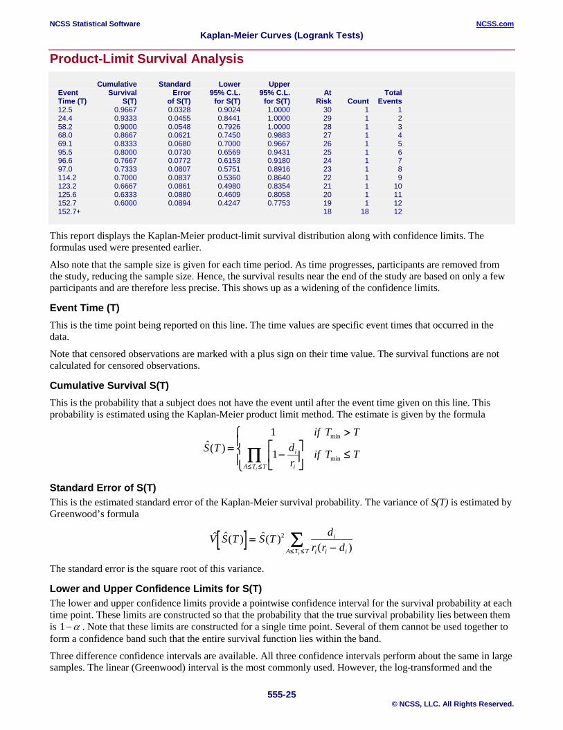
Product-Limit Survival Analysis Cumulative Standard Lower Upper
Event Survival Error 95% C.L. 95% C.L. At Total Time (T) S(T) of S(T) for S(T) for S(T) Risk Count Events 12.5 0.9667 0.0328 0.9024 1.0000 30 1 1 24.4 0.9333 0.0455 0.8441 1.0000 29 1 2 58.2 0.9000 0.0548 0.7926 1.0000 28 1 3 68.0 0.8667 0.0621 0.7450 0.9883 27 1 4 69.1 0.8333 0.0680 0.7000 0.9667 26 1 5 95.5 0.8000 0.0730 0.6569 0.9431 25 1 6 96.6 0.7667 0.0772 0.6153 0.9180 24 1 7 97.0 0.7333 0.0807 0.5751 0.8916 23 1 8 114.2 0.7000 0.0837 0.5360 0.8640 22 1 9 123.2 0.6667 0.0861 0.4980 0.8354 21 1 10 125.6 0.6333 0.0880 0.4609 0.8058 20 1 11 152.7 0.6000 0.0894 0.4247 0.7753 19 1 12 152.7+ 18 18 12
This report displays the Kaplan-Meier product-limit survival distribution along with confidence limits. The formulas used were presented earlier.
Also note that the sample size is given for each time period. As time progresses, participants are removed from the study, reducing the sample size. Hence, the survival results near the end of the study are based on only a few participants and are therefore less precise. This shows up as a widening of the confidence limits.
Event Time (T) This is the time point being reported on this line. The time values are specific event times that occurred in the data.
Note that censored observations are marked with a plus sign on their time value. The survival functions are not calculated for censored observations.
Cumulative Survival S(T) This is the probability that a subject does not have the event until after the event time given on this line. This probability is estimated using the Kaplan-Meier product limit method. The estimate is given by the formula
( )min
minS T
if T Tdr
if T Ti
iA T Ti
=>
−
≤
≤ ≤∏
1
1
Standard Error of S(T) This is the estimated standard error of the Kaplan-Meier survival probability. The variance of S(T) is estimated by Greenwood’s formula
[ ] ( ) ( )( )
V S T S T dr r d
i
i i iA T Ti
=−≤ ≤
∑2
The standard error is the square root of this variance.
Lower and Upper Confidence Limits for S(T) The lower and upper confidence limits provide a pointwise confidence interval for the survival probability at each time point. These limits are constructed so that the probability that the true survival probability lies between them is α−1 . Note that these limits are constructed for a single time point. Several of them cannot be used together to form a confidence band such that the entire survival function lies within the band.
Three difference confidence intervals are available. All three confidence intervals perform about the same in large samples. The linear (Greenwood) interval is the most commonly used. However, the log-transformed and the
NCSS Statistical Software NCSS.com Kaplan-Meier Curves (Logrank Tests)
555-26 © NCSS, LLC. All Rights Reserved.
arcsine-square intervals behave better in small to moderate samples, so they are recommended. The formulas for these limits were given at the beginning of the chapter and are not repeated here.
At Risk This value is the number of individuals at risk. The number at risk is all those under study who died or were censored at a time later than the current time. As the number of individuals at risk is decreased, the estimates become less reliable.
Count This is the number of individuals having the event (failing) at this time point.
Total Events This is the cumulative number of individuals having the event (failing) up to and including this time value.
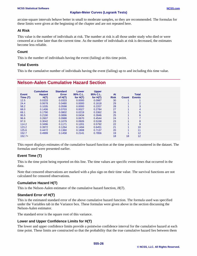
Nelson-Aalen Cumulative Hazard Section
Cumulative Standard Lower Upper Event Hazard Error 95% C.L. 95% C.L. At Total Time (T) H(T) of H(T) for H(T) for H(T) Risk Count Events 12.5 0.0333 0.0333 0.0000 0.0987 30 1 1 24.4 0.0678 0.0480 0.0000 0.1618 29 1 2 58.2 0.1035 0.0598 0.0000 0.2207 28 1 3 68.0 0.1406 0.0703 0.0027 0.2784 27 1 4 69.1 0.1790 0.0802 0.0219 0.3362 26 1 5 95.5 0.2190 0.0896 0.0434 0.3946 25 1 6 96.6 0.2607 0.0988 0.0670 0.4544 24 1 7 97.0 0.3042 0.1079 0.0926 0.5158 23 1 8 114.2 0.3496 0.1171 0.1201 0.5792 22 1 9 123.2 0.3972 0.1264 0.1494 0.6451 21 1 10 125.6 0.4472 0.1360 0.1808 0.7137 20 1 11 152.7 0.4999 0.1458 0.2141 0.7856 19 1 12 152.7+ 18 18 12
This report displays estimates of the cumulative hazard function at the time points encountered in the dataset. The formulas used were presented earlier.
Event Time (T) This is the time point being reported on this line. The time values are specific event times that occurred in the data.
Note that censored observations are marked with a plus sign on their time value. The survival functions are not calculated for censored observations.
Cumulative Hazard H(T) This is the Nelson-Aalen estimator of the cumulative hazard function, H(T).
Standard Error of H(T) This is the estimated standard error of the above cumulative hazard function. The formula used was specified under the Variables tab in the Variance box. These formulas were given above in the section discussing the Nelson-Aalen estimator.
The standard error is the square root of this variance.
Lower and Upper Confidence Limits for H(T) The lower and upper confidence limits provide a pointwise confidence interval for the cumulative hazard at each time point. These limits are constructed so that the probability that the true cumulative hazard lies between them
NCSS Statistical Software NCSS.com Kaplan-Meier Curves (Logrank Tests)
555-27 © NCSS, LLC. All Rights Reserved.
is 1− α . Note that these limits are constructed for a single time point. Several of them cannot be used together to form a confidence band such that the entire cumulative hazard function lies within the band.
Three difference confidence intervals are available. All three confidence intervals perform about the same in large samples. The linear (Greenwood) interval is the most commonly used. However, the log-transformed and the arcsine-square intervals behave better in small to moderate samples, so they are recommended. The formulas for these limits were given at the beginning of the chapter and are not repeated here.
At Risk This value is the number of individuals at risk. The number at risk is all those under study who died or were censored at a time later than the current time. As the number of individuals at risk is decreased, the estimates become less reliable.
Count This is the number of individuals having the event (failing) at this time point.
Total Events This is the cumulative number of individuals having the event (failing) up to and including this time value.
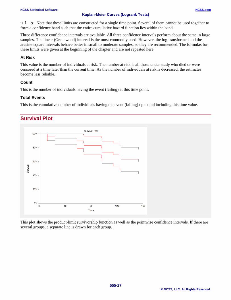
Survival Plot
This plot shows the product-limit survivorship function as well as the pointwise confidence intervals. If there are several groups, a separate line is drawn for each group.
NCSS Statistical Software NCSS.com Kaplan-Meier Curves (Logrank Tests)
555-28 © NCSS, LLC. All Rights Reserved.
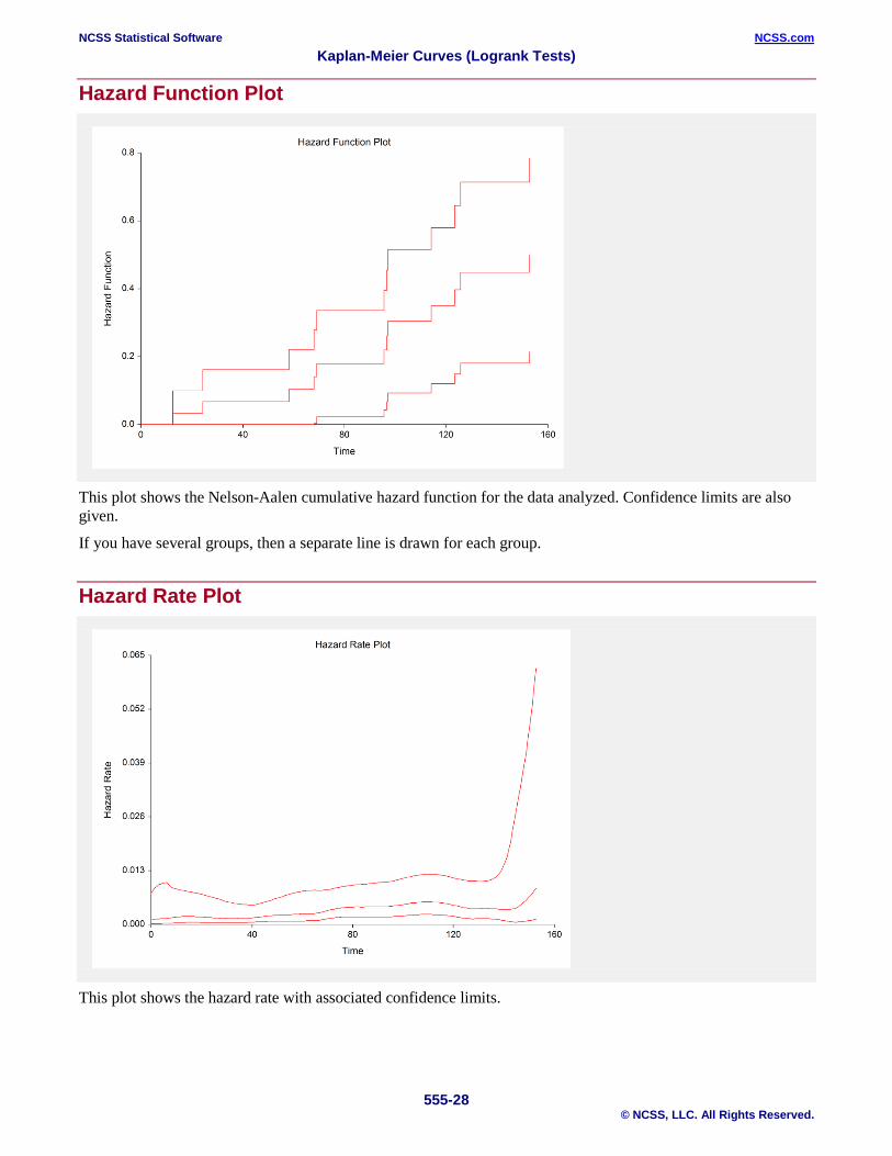
Hazard Function Plot
This plot shows the Nelson-Aalen cumulative hazard function for the data analyzed. Confidence limits are also given.
If you have several groups, then a separate line is drawn for each group.
Hazard Rate Plot
This plot shows the hazard rate with associated confidence limits.

NCSS Statistical Software NCSS.com Kaplan-Meier Curves (Logrank Tests)
555-29 © NCSS, LLC. All Rights Reserved.
Example 2 – Logrank Tests This section presents an example of how to use a logrank test to compare the hazard rates of two or more groups. The data used are recorded in the variables Tumor6, Censor6, and Trtmnt6 of the Survival dataset. You may follow along here by making the appropriate entries or load the completed template Example 2 by clicking on Open Example Template from the File menu of the Kaplan-Meier Curves (Logrank Tests) Fitting window.
1 Open the Survival dataset. • From the File menu of the NCSS Data window, select Open Example Data. • Click on the file Survival.NCSS. • Click Open.
2 Open the Kaplan-Meier Curves (Logrank Tests) window. • Using the Analysis menu or the Procedure Navigator, find and select the Kaplan-Meier Curves
(Logrank Tests) procedure. • On the menus, select File, then New Template. This will fill the procedure with the default template.
3 Specify the variables. • On the Kaplan-Meier Curves (Logrank Tests) window, select the Variables tab. • Set the Time Variable to Tumor6. • Set the Censor Variable to Censor6. • Set the Group Variable to Trtmnt6. • Check the Run Randomization Tests box. • Set the Monte Carlo Samples to 1000.
4 Run the procedure. • From the Run menu, select Run Procedure. Alternatively, just click the green Run button.
Logrank Tests Section Randomization Weighting Test of Hazard Prob Prob Comparisons Test Name Chi-Square DF Level* Level* Across Time Logrank 4.996 1 0.0254 0.0470 Equal Gehan-Wilcoxon 3.956 1 0.0467 0.0520 High++ to Low++ Tarone-Ware 4.437 1 0.0352 0.0510 High to Low Peto-Peto 3.729 1 0.0535 0.0670 High+ to Low+ Mod. Peto-Peto 3.618 1 0.0572 0.0740 High+ to Low+ F-H (1, 0) 3.956 1 0.0467 0.0520 Almost Equal F-H (.5, .5) 3.507 1 0.0611 0.0920 Low+ to High+ F-H (1, 1) 4.024 1 0.0449 0.0760 Low to High F-H (0, 1) 5.212 1 0.0224 0.0650 Low to High F-H (.5, 2) 5.942 1 0.0148 0.0420 Low++ to High++ *These probability levels are only valid when a single test was selected before this analysis is seen. You cannot select a test to report after viewing this table without adding bias to the results. Unless you have good reason to do otherwise, you should use the equal weighting (logrank) test.
This report gives the results of the ten logrank type tests that are provided by this procedure. We strongly suggest that you select the test that will be used before viewing this report. Unless you have a good reason for doing so, we recommend that you use the first (Logrank) test.
NCSS Statistical Software NCSS.com Kaplan-Meier Curves (Logrank Tests)
555-30 © NCSS, LLC. All Rights Reserved.
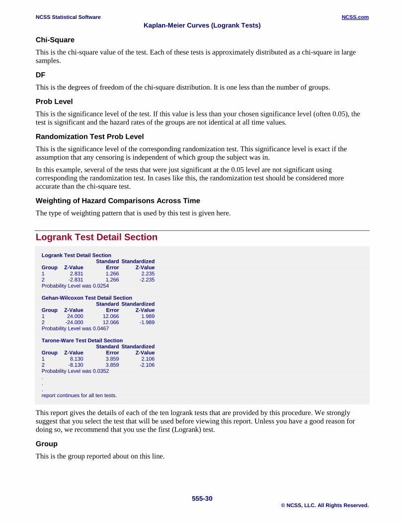
Chi-Square This is the chi-square value of the test. Each of these tests is approximately distributed as a chi-square in large samples.
DF This is the degrees of freedom of the chi-square distribution. It is one less than the number of groups.
Prob Level This is the significance level of the test. If this value is less than your chosen significance level (often 0.05), the test is significant and the hazard rates of the groups are not identical at all time values.
Randomization Test Prob Level This is the significance level of the corresponding randomization test. This significance level is exact if the assumption that any censoring is independent of which group the subject was in.
In this example, several of the tests that were just significant at the 0.05 level are not significant using corresponding the randomization test. In cases like this, the randomization test should be considered more accurate than the chi-square test.
Weighting of Hazard Comparisons Across Time The type of weighting pattern that is used by this test is given here.
Logrank Test Detail Section
Logrank Test Detail Section Standard Standardized Group Z-Value Error Z-Value 1 2.831 1.266 2.235 2 -2.831 1.266 -2.235 Probability Level was 0.0254 Gehan-Wilcoxon Test Detail Section Standard Standardized Group Z-Value Error Z-Value 1 24.000 12.066 1.989 2 -24.000 12.066 -1.989 Probability Level was 0.0467 Tarone-Ware Test Detail Section Standard Standardized Group Z-Value Error Z-Value 1 8.130 3.859 2.106 2 -8.130 3.859 -2.106 Probability Level was 0.0352 . . . report continues for all ten tests.
This report gives the details of each of the ten logrank tests that are provided by this procedure. We strongly suggest that you select the test that will be used before viewing this report. Unless you have a good reason for doing so, we recommend that you use the first (Logrank) test.
Group This is the group reported about on this line.

NCSS Statistical Software NCSS.com Kaplan-Meier Curves (Logrank Tests)
555-31 © NCSS, LLC. All Rights Reserved.
Z-Value This is a weighted average of the difference between the observed hazard rates of this group and the expected hazard rates under the null hypothesis of hazard rate equality. The expected hazard rates are found by computing new hazard rates based on all that data as if they all came from a single group.
By considering the magnitudes of these values, you can determine which group (or groups) are different from the rest.
Standard Error This is the standard error of the above z-value. It is used to standardize the z-values.
Standardized Z-Value The standardized z-value is created by dividing the z-value by its standard error. This provides an index number that will usually very between -3 and 3. Larger values represent groups that quite different from the typical group, at least at some time values.
Hazard Ratio Detail Section Cox- Mantel Sample Observed Expected Hazard Hazard Hyper. Size Events Events Rates Ratio Var. Groups (nA/nB) (OA/OB) (EA/EB) (HRA/HRB) (HR) (V) 1/2 6/6 6/4 3.17/6.83 1.89/0.59 3.23 1.60 2/1 6/6 4/6 6.83/3.17 0.59/1.89 0.31 1.60
This report gives the details of the hazard ratio calculation. One line of the report is devoted to each pair of groups.
Groups These are the two groups reported about on this line, separated by a slash.
Sample Size These are the sample sizes of the two groups.
Observed Events These are the number of events (deaths) observed in the two groups.
Expected Events These are the number of events (deaths) expected in each group under the hypothesis that the two hazard rates are equal.
Hazard Rates These are the hazard rates of the two groups. The hazard rate is computed as the ratio of the number of observed and expected events.
Cox-Mantel Hazard Ratio This is the value of the Cox-Mantel hazard ratio. This is the ratio of the two hazard rates.
Hyper. Var. This is the value of V, the hypergeometric variance. This value is used to compute the Mantel-Haenszel hazard ratio and confidence interval.
NCSS Statistical Software NCSS.com Kaplan-Meier Curves (Logrank Tests)
555-32 © NCSS, LLC. All Rights Reserved.
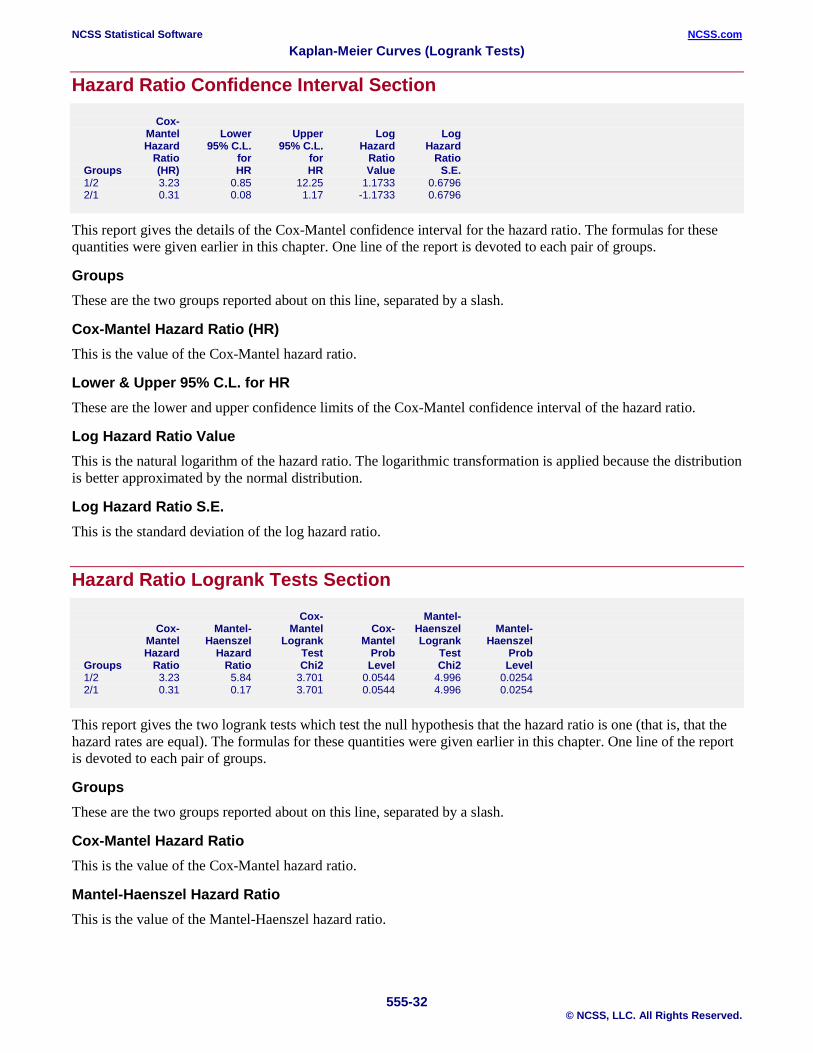
Hazard Ratio Confidence Interval Section Cox- Mantel Lower Upper Log Log Hazard 95% C.L. 95% C.L. Hazard Hazard Ratio for for Ratio Ratio Groups (HR) HR HR Value S.E. 1/2 3.23 0.85 12.25 1.1733 0.6796 2/1 0.31 0.08 1.17 -1.1733 0.6796
This report gives the details of the Cox-Mantel confidence interval for the hazard ratio. The formulas for these quantities were given earlier in this chapter. One line of the report is devoted to each pair of groups.
Groups These are the two groups reported about on this line, separated by a slash.
Cox-Mantel Hazard Ratio (HR) This is the value of the Cox-Mantel hazard ratio.
Lower & Upper 95% C.L. for HR These are the lower and upper confidence limits of the Cox-Mantel confidence interval of the hazard ratio.
Log Hazard Ratio Value This is the natural logarithm of the hazard ratio. The logarithmic transformation is applied because the distribution is better approximated by the normal distribution.
Log Hazard Ratio S.E. This is the standard deviation of the log hazard ratio.
Hazard Ratio Logrank Tests Section Cox- Mantel- Cox- Mantel- Mantel Cox- Haenszel Mantel- Mantel Haenszel Logrank Mantel Logrank Haenszel Hazard Hazard Test Prob Test Prob Groups Ratio Ratio Chi2 Level Chi2 Level 1/2 3.23 5.84 3.701 0.0544 4.996 0.0254 2/1 0.31 0.17 3.701 0.0544 4.996 0.0254
This report gives the two logrank tests which test the null hypothesis that the hazard ratio is one (that is, that the hazard rates are equal). The formulas for these quantities were given earlier in this chapter. One line of the report is devoted to each pair of groups.
Groups These are the two groups reported about on this line, separated by a slash.
Cox-Mantel Hazard Ratio This is the value of the Cox-Mantel hazard ratio.
Mantel-Haenszel Hazard Ratio This is the value of the Mantel-Haenszel hazard ratio.

NCSS Statistical Software NCSS.com Kaplan-Meier Curves (Logrank Tests)
555-33 © NCSS, LLC. All Rights Reserved.
Cox-Mantel Logrank Test This is the test statistic for the Cox-Mantel logrank test. This value is approximately distributed as a chi-square with one degree of freedom.
Note that this test is more commonly used than the Mantel-Haenszel test.
Cox-Mantel Prob Level This is the significance level of the Cox-Mantel logrank test. The hypothesis of hazard rate equality is rejected if this value is less than 0.05 (or 0.01).
Mantel-Haenszel Logrank Test This is the test statistic for the Mantel-Haenszel logrank test. This value is approximately distributed as a chi-square with one degree of freedom.
Mantel-Haenszel Prob Level This is the significance level of the Mantel-Haenszel logrank test. The hypothesis of hazard rate equality is rejected if this value is less than 0.05 (or 0.01).

NCSS Statistical Software NCSS.com Kaplan-Meier Curves (Logrank Tests)
555-34 © NCSS, LLC. All Rights Reserved.
Example 3 – Validation of Kaplan-Meier Product Limit Estimator using Collett (1994) This section presents validation of the Kaplan-Meier product limit estimator and associated statistics. Collett (1994) presents an example on page 5 of the time to discontinuation of use of an IUD. The data are as follows: 10, 13+, 18+, 19, 23+, 30, 36, 38+, 54+, 56+, 59, 75, 93, 97, 104+, 107, 107+, 107+. These data are contained in the Collett dataset. On page 26, Collett (1994) gives the product-limit estimator, its standard deviation, and 95% confidence interval. A partial list of these results is given here: Time S(T) s.e. 95% C.I 10 0.9444 0.0540 (0.839, 1.000) 36 0.7459 0.1170 (0.529, 0.963) 93 0.4662 0.1452 (0.182, 0.751) 107 0.2486 0.1392 (0.000, 0.522) We will now run these data through this procedure to see that NCSS gets these same results. You may follow along here by making the appropriate entries or load the completed template Example 3 by clicking on Open Example Template from the File menu of the Kaplan-Meier Curves (Logrank Tests) Fitting window.
1 Open the Collett5 dataset. • From the File menu of the NCSS Data window, select Open Example Data. • Click on the file Collett5.NCSS. • Click Open.
2 Open the Kaplan-Meier Curves (Logrank Tests) window. • Using the Analysis menu or the Procedure Navigator, find and select the Kaplan-Meier Curves
(Logrank Tests) procedure. • On the menus, select File, then New Template. This will fill the procedure with the default template.
3 Specify the variables. • On the Kaplan-Meier Curves (Logrank Tests) window, select the Variables tab. • Set the Time Variable to Time. • Set the Censor Variable to Censor.
4 Specify the reports. • On the Kaplan-Meier Curves (Logrank Tests) window, select the Reports tab. • Uncheck all reports except the Kaplan-Meier Detail report.
5 Run the procedure. • From the Run menu, select Run Procedure. Alternatively, just click the green Run button.
NCSS Statistical Software NCSS.com Kaplan-Meier Curves (Logrank Tests)
555-35 © NCSS, LLC. All Rights Reserved.
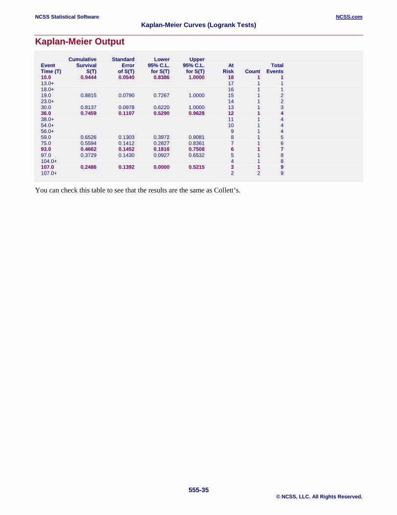
Kaplan-Meier Output Cumulative Standard Lower Upper
Event Survival Error 95% C.L. 95% C.L. At Total Time (T) S(T) of S(T) for S(T) for S(T) Risk Count Events 10.0 0.9444 0.0540 0.8386 1.0000 18 1 1 13.0+ 17 1 1 18.0+ 16 1 1 19.0 0.8815 0.0790 0.7267 1.0000 15 1 2 23.0+ 14 1 2 30.0 0.8137 0.0978 0.6220 1.0000 13 1 3 36.0 0.7459 0.1107 0.5290 0.9628 12 1 4 38.0+ 11 1 4 54.0+ 10 1 4 56.0+ 9 1 4 59.0 0.6526 0.1303 0.3972 0.9081 8 1 5 75.0 0.5594 0.1412 0.2827 0.8361 7 1 6 93.0 0.4662 0.1452 0.1816 0.7508 6 1 7 97.0 0.3729 0.1430 0.0927 0.6532 5 1 8 104.0+ 4 1 8 107.0 0.2486 0.1392 0.0000 0.5215 3 1 9 107.0+ 2 2 9
You can check this table to see that the results are the same as Collett’s.

NCSS Statistical Software NCSS.com Kaplan-Meier Curves (Logrank Tests)
555-36 © NCSS, LLC. All Rights Reserved.
Example 4 – Validation of Nelson-Aalen Estimator using Klein and Moeschberger (1997) This section presents validation of the Nelson-Aalen estimator and associated statistics. Klein and Moeschberger (1997) present an example of output for the cumulative hazard function on page 89. The data are available on their website. These data are contained in the BMT dataset. A partial list of these results for the ALL group (our group 1) is given here: Time H(T) s.e. 1 0.0263 0.0263 332 0.5873 0.1449 662 1.0152 0.2185 We will now run these data through this procedure to see that NCSS gets these same results. You may follow along here by making the appropriate entries or load the completed template Example 4 by clicking on Open Example Template from the File menu of the Kaplan-Meier Curves (Logrank Tests) Fitting window. 1 Open the BMT dataset.
• From the File menu of the NCSS Data window, select Open Example Data. • Click on the file BMT.NCSS. • Click Open.
2 Open the Kaplan-Meier Curves (Logrank Tests) window. • Using the Analysis menu or the Procedure Navigator, find and select the Kaplan-Meier Curves
(Logrank Tests) procedure. • On the menus, select File, then New Template. This will fill the procedure with the default template.
3 Specify the variables. • On the Kaplan-Meier Curves (Logrank Tests) window, select the Variables tab. • Set the Time Variable to Time. • Set the Censor Variable to D3. • Set the Group Variable to Group.
4 Specify the reports. • On the Kaplan-Meier Curves (Logrank Tests) window, select the Reports tab. • Uncheck all reports except the Cumulative Hazard Detail report.
5 Run the procedure. • From the Run menu, select Run Procedure. Alternatively, just click the green Run button.
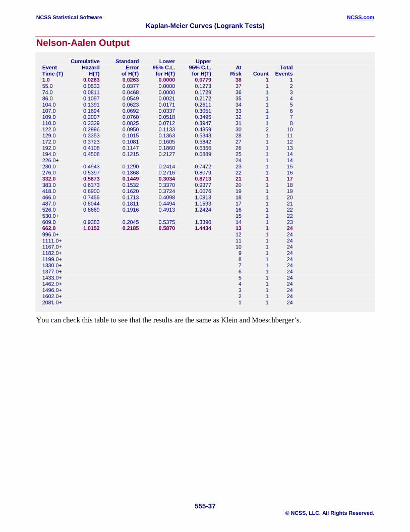
NCSS Statistical Software NCSS.com Kaplan-Meier Curves (Logrank Tests)
555-37 © NCSS, LLC. All Rights Reserved.
Nelson-Aalen Output
Cumulative Standard Lower Upper Event Hazard Error 95% C.L. 95% C.L. At Total Time (T) H(T) of H(T) for H(T) for H(T) Risk Count Events 1.0 0.0263 0.0263 0.0000 0.0779 38 1 1 55.0 0.0533 0.0377 0.0000 0.1273 37 1 2 74.0 0.0811 0.0468 0.0000 0.1729 36 1 3 86.0 0.1097 0.0549 0.0021 0.2172 35 1 4 104.0 0.1391 0.0623 0.0171 0.2611 34 1 5 107.0 0.1694 0.0692 0.0337 0.3051 33 1 6 109.0 0.2007 0.0760 0.0518 0.3495 32 1 7 110.0 0.2329 0.0825 0.0712 0.3947 31 1 8 122.0 0.2996 0.0950 0.1133 0.4859 30 2 10 129.0 0.3353 0.1015 0.1363 0.5343 28 1 11 172.0 0.3723 0.1081 0.1605 0.5842 27 1 12 192.0 0.4108 0.1147 0.1860 0.6356 26 1 13 194.0 0.4508 0.1215 0.2127 0.6889 25 1 14 226.0+ 24 1 14 230.0 0.4943 0.1290 0.2414 0.7472 23 1 15 276.0 0.5397 0.1368 0.2716 0.8079 22 1 16 332.0 0.5873 0.1449 0.3034 0.8713 21 1 17 383.0 0.6373 0.1532 0.3370 0.9377 20 1 18 418.0 0.6900 0.1620 0.3724 1.0076 19 1 19 466.0 0.7455 0.1713 0.4098 1.0813 18 1 20 487.0 0.8044 0.1811 0.4494 1.1593 17 1 21 526.0 0.8669 0.1916 0.4913 1.2424 16 1 22 530.0+ 15 1 22 609.0 0.9383 0.2045 0.5375 1.3390 14 1 23 662.0 1.0152 0.2185 0.5870 1.4434 13 1 24 996.0+ 12 1 24 1111.0+ 11 1 24 1167.0+ 10 1 24 1182.0+ 9 1 24 1199.0+ 8 1 24 1330.0+ 7 1 24 1377.0+ 6 1 24 1433.0+ 5 1 24 1462.0+ 4 1 24 1496.0+ 3 1 24 1602.0+ 2 1 24 2081.0+ 1 1 24
You can check this table to see that the results are the same as Klein and Moeschberger’s.
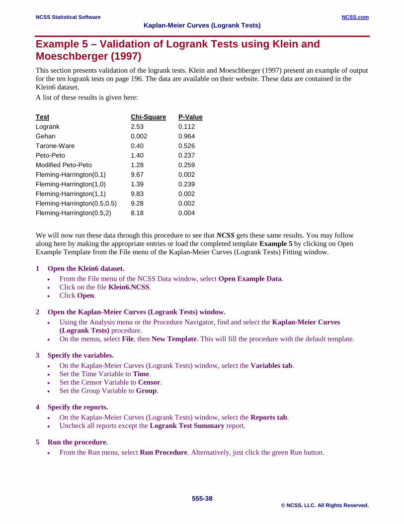
NCSS Statistical Software NCSS.com Kaplan-Meier Curves (Logrank Tests)
555-38 © NCSS, LLC. All Rights Reserved.
Example 5 – Validation of Logrank Tests using Klein and Moeschberger (1997) This section presents validation of the logrank tests. Klein and Moeschberger (1997) present an example of output for the ten logrank tests on page 196. The data are available on their website. These data are contained in the Klein6 dataset. A list of these results is given here: Test Chi-Square P-Value Logrank 2.53 0.112 Gehan 0.002 0.964 Tarone-Ware 0.40 0.526 Peto-Peto 1.40 0.237 Modified Peto-Peto 1.28 0.259 Fleming-Harrington(0,1) 9.67 0.002 Fleming-Harrington(1,0) 1.39 0.239 Fleming-Harrington(1,1) 9.83 0.002 Fleming-Harrington(0.5,0.5) 9.28 0.002 Fleming-Harrington(0.5,2) 8.18 0.004
We will now run these data through this procedure to see that NCSS gets these same results. You may follow along here by making the appropriate entries or load the completed template Example 5 by clicking on Open Example Template from the File menu of the Kaplan-Meier Curves (Logrank Tests) Fitting window.
1 Open the Klein6 dataset. • From the File menu of the NCSS Data window, select Open Example Data. • Click on the file Klein6.NCSS. • Click Open.
2 Open the Kaplan-Meier Curves (Logrank Tests) window. • Using the Analysis menu or the Procedure Navigator, find and select the Kaplan-Meier Curves
(Logrank Tests) procedure. • On the menus, select File, then New Template. This will fill the procedure with the default template.
3 Specify the variables. • On the Kaplan-Meier Curves (Logrank Tests) window, select the Variables tab. • Set the Time Variable to Time. • Set the Censor Variable to Censor. • Set the Group Variable to Group.
4 Specify the reports. • On the Kaplan-Meier Curves (Logrank Tests) window, select the Reports tab. • Uncheck all reports except the Logrank Test Summary report.
5 Run the procedure. • From the Run menu, select Run Procedure. Alternatively, just click the green Run button.

NCSS Statistical Software NCSS.com Kaplan-Meier Curves (Logrank Tests)
555-39 © NCSS, LLC. All Rights Reserved.
Logrank Test Output Randomization Weighting Test of Hazard Prob Prob Comparisons Test Name Chi-Square DF Level* Level* Across Time Logrank 2.530 1 0.1117 Equal Gehan-Wilcoxon 0.002 1 0.9636 High++ to Low++ Tarone-Ware 0.403 1 0.5257 High to Low Peto-Peto 1.399 1 0.2369 High+ to Low+ Mod. Peto-Peto 1.276 1 0.2587 High+ to Low+ F-H (1, 0) 1.387 1 0.2390 Almost Equal F-H (.5, .5) 9.285 1 0.0023 Low+ to High+ F-H (1, 1) 9.834 1 0.0017 Low to High F-H (0, 1) 9.668 1 0.0019 Low to High F-H (.5, 2) 8.179 1 0.0042 Low++ to High++
You can check this table to see that the results are the same as Klein and Moeschberger’s. Note that the order of the tests is different.
Also note that the randomization test probability levels will change slightly from run to run because they are based on Monte Carlo sampling.