1

Fabrication and characterization of perpendicular magnetic anisotropy thin-film CoCrPt grown

on a Ti underlayer

by

Margaret Marie Kane

Submitted to the Department of Materials Science and Engineering

in Partial Fulfillment of the Requirements for the Degree of

Bachelor of Science

at the

Massachusetts Institute of Technology

June 2015

© 2015 Margaret Kane All rights reserved

The author hereby grants to MIT permission to reproduce and to distribute publicly paper and electronic copies of the thesis document in whole or in part in any medium know or hereafter

created.

Signature of Author………………………….………………………………………………...........

Department of Materials Science and Engineering 05/01/2015

Certified by…………………………………………………………………………………………

Caroline Ross Toyota Professor of Materials Science and Engineering

Thesis Supervisor Accepted by ………………………..………………………………………………………………

Geoffrey Beach Class of ‘58’ Associate Professor of Materials Science and Engineering

Chairman, Undergraduate Thesis Committee

 

2

Fabrication and characterization of perpendicular magnetic anisotropy thin-film CoCrPt grown on a Ti underlayer

by

Margaret Marie Kane

Submitted to the Department of Materials Science and Engineering on May 1, 2015 in Partial Fulfillment of the Requirements for the Degree of Bachelor of Science

in Materials Science and Engineering

 ABSTRACT   CoCrPt has potential applications as a memory storage technology because of its perpendicular magnetic anisotropy (PMA) characteristics. An underlayer can be used to ensure the out-of-plane magnetization required for PMA functionalities. Ti, with a lattice constant of a = 2.95 Å can be used to encourage uniaxial c-axis growth in CoCrPt (lattice constant a ≅ 2.55 Å, dependent on exact composition). In this report, varying thicknesses of Ti (t = 0, 20, 40, 60, 70, 80, 90, 100nm) and CoCrPt (t = 50, 75, 90, 100, 125, 150nm) were sputtered onto naturally oxidized silicon substrates. Using various characterization methods, these films were investigated in order to better understand the system. The exact composition of the CoCrPt films was found to be approximately Co60.2Cr16.4Pt23.4, with a Curie temperature of about 600 ºC. The addition of a Ti underlayer resulted in an increase in coercivity to approximately 1250 Oe for t > 60nm. However, switching field distribution and saturation magnetization appear to be independent of underlayer thickness. All samples show evidence of out-of-plane growth and the roughness of the films increases until it also plateaus at about t = 60nm. When CoCrPt thickness is varied on a constant Ti underlayer, the PMA properties of the materials decrease with increasing thickness due to increased disorder and potential relaxation of the lattice in thicker films. The switching field distribution shows a significant increase, implying that a thicker film has a more homogenous distribution of grain sizes. XRD peaks confirm out-of-plane growth and suggest a trend of increasing c lattice constant as the thickness of the film increases. Thesis Supervisor: Caroline Ross Title: Toyota Professor of Materials Science and Engineering

 

3

ACKNOWLEDGEMENTS  I would like to first thank Dr. Pin Ho and Professor Caroline Ross for their invaluable help with this thesis. Thank you Libby Shaw, Donald Galler, Kun-Hua Tu for training me to use the instruments instrumental to my completion of this thesis. I also need to thank all the professors and lab instructors I’ve had at MIT who both inspired me and taught me the skills I now use on a regular basis. Thanks to my parents and sisters for their support and love.    

 

4

TABLE  OF  CONTENTS  ABSTRACT _________________________________________________________________ 2

ACKNOWLEDGEMENTS _____________________________________________________ 3

TABLE OF CONTENTS _______________________________________________________ 4

TABLE OF FIGURES _________________________________________________________ 5

TABLE OF TABLES __________________________________________________________ 6

INTRODUCTION ____________________________________________________________ 7 MAGNETIC ANISOTROPY ______________________________________________________ 9 PERPENDICULAR MAGNETIC ANISOTROPY ________________________________________ 12 COBALT CHROMIUM PLATINUM THIN FILMS ______________________________________ 13 OBJECTIVES _______________________________________________________________ 16

EXPERIMENTAL DESIGN AND METHODS ____________________________________ 16 SAMPLE PREPARATION _______________________________________________________ 16 SAMPLE ANALYSIS __________________________________________________________ 18

Energy-Dispersive X-Ray Spectrometer _______________________________________ 18 Vibrating Sample Magnetometer _____________________________________________ 19 X-Ray Diffractometer _____________________________________________________ 23 Atomic Force Microscope __________________________________________________ 24

RESULTS AND DISCUSSION _________________________________________________ 25 COMPOSITION AND MAGNETIC PROPERTIES OF COCRPT ______________________________ 25

Composition _____________________________________________________________ 25 Curie temperature ________________________________________________________ 28

EFFECTS OF VARYING TI UNDERLAYER THICKNESS _________________________________ 34 Magnetic Properties ______________________________________________________ 34 Crystallography __________________________________________________________ 39 Topography _____________________________________________________________ 42

EFFECTS OF VARYING COCRPT FILM THICKNESS ___________________________________ 43 Magnetic Properties ______________________________________________________ 44 Crystallography __________________________________________________________ 50 Topography _____________________________________________________________ 53

CONCLUSION AND FURTHER WORK _________________________________________ 54

WORKS CITED _____________________________________________________________ 57

 

5

TABLE  OF  FIGURES  FIGURE 1. RECORDING MEDIUM GEOMETRIES. (A) TAPES, LINEAR RECORDING; (B) MODERN HARD

DRIVE, CIRCUMFERENTIAL RECORDING ..................................................................................... 7 FIGURE 2. RACETRACK MEMORY SCHEMATIC .................................................................................. 8 FIGURE 3. MAGNETIC RANDOM ACCESS MEMORY SPIN VALVE ......................................................... 9 FIGURE 4. CRYSTALLOGRAPHIC AND MAGNETIC PROPERTIES OF COBALT. (A) HEXAGONAL CLOSE

PACKED CRYSTAL STRUCTURE OF COBALT WITH ANNOTATED EASY AND HARD AXIS; (B)

REACTION OF THE MAGNETIZATION OF COBALT TO AN APPLIED FIELD ALONG THE HARD AND

EASY AXIS ............................................................................................................................... 11 FIGURE 5. SCHEMATIC OF A VIBRATING SAMPLE MAGNETOMETER. ............................................... 19 FIGURE 6. STANDARD HYSTERESIS LOOP FOR A MAGNETIC MATERIAL. MS DENOTES THE

SATURATION MAGNETIZATION, HC THE COERCIVITY, AND MR THE REMANENCE. .................... 20 FIGURE 7. SCHEMATIC OF AN X-RAY DIFFRACTOMETER. ................................................................ 23 FIGURE 8. IN-PLANE AND OUT-OF-PLANE HYSTERESIS LOOPS FOR CO60.2CR16.4PT23.4 (T = 90NM) ON

BARE, NATURALLY OXIDIZED SI .............................................................................................. 28 FIGURE 9. OUT-OF PLANE M-H CURVES FOR COCRPT THIN FILMS (T = 140NM) AT DIFFERENT

TEMPERATURES, AS LABELED ................................................................................................. 30 FIGURE 10. MAGNETIC PROPERTIES OF COCRPT (T = 140NM) FOR DIFFERENT TEMPERATURES ..... 31 FIGURE 11. OUT-OF LOOP HYSTERESIS LOOPS FOR COCRPT (T = 140NM) FILMS WITH NO POST-

FABRICATION TREATMENT AND ANNEALING AT 500ºC FOR APPROXIMATELY 40 MINUTES ..... 33 FIGURE 12. M-H CURVES FOR COCRPT THIN FILMS (T = 90NM) WITH VARYING TI UNDERLAYER

THICKNESS .............................................................................................................................. 35 FIGURE 13. THE OUT-OF-PLANE MAGNETIC PROPERTIES OF COCRPT (T = 90NM) AND VARIABLE TI

UNDERLAYER THICKNESS (T = 20, 40, 60, 70, 80, 90, 100NM) ................................................. 36 FIGURE 14. XRD SCANS FOR 90NM COCRPT FILMS WITH VARYING TI UNDERLAYER THICKNESS (T =

20, 40, 60, 70, 80, 90, 100NM) ................................................................................................ 40 FIGURE 15. TREND OF ROUGHNESS MEASURED FOR SAMPLES WITH CONSTANT THICKNESS COCRPT

LAYERS (T = 90NM) AND VARYING THICKNESS TI LAYERS ...................................................... 43 FIGURE 16. OUT-OF PLANE M-H CURVES FOR CONSTANT TI UNDERLAYER (T = 80NM) WITH

VARYING COCRPT FILM THICKNESS ....................................................................................... 45 FIGURE 17. THE OUT-OF-PLANE MAGNETIC PROPERTIES OF COCRPT (T = 50, 75, 100, 125, 150NM)

AND CONSTANT TI UNDERLAYER THICKNESS (T = 80NM). ....................................................... 47 FIGURE 18. XRD SCANS FOR VARYING THICKNESS COCRPT FIMS (T = 50, 75, 90, 100, 125, 150NM)

AND AN 80NM TI UNDERLAYER ............................................................................................... 51 FIGURE 19. TREND OF ROUGHNESS MEASURED FOR SAMPLES WITH VARYING THICKNESS COCRPT

LAYERS AND CONSTANT THICKNESS TI LAYERS (T = 80NM) .................................................... 53

 

6

TABLE  OF  TABLES  TABLE 1. MEASURED DEPOSITION RATES ....................................................................................... 17

TABLE 2. SAMPLES PREPARED USING DC MAGNETRON SPUTTERING ............................................... 18

TABLE 3. COMPOSITION OF COCRPT THIN FILMS CREATED BY SPUTTERING OFF A CO66CR22PT12

TARGET. .................................................................................................................................. 26

TABLE 4. GAUSSIAN FITS USED TO CALCULATE THE SWITCHING FIELD DISTRIBUTION OF SAMPLES

WITH VARYING TI UNDERLAYER THICKNESSES ....................................................................... 39

TABLE 5. CRYSTALLOGRAPHIC VALUES ACQUIRED WITH XRD SCANS (STEP SIZE 0.0167º) FOR

VARYING TI UNDERLAYER THICKNESS (T = 20, 40, 60, 70, 80, 90, 100NM) ............................. 41

TABLE 6. GAUSSIAN FITS USED TO CALCULATE THE SWITCHING FIELD DISTRIBUTION OF SAMPLES

WITH VARYING COCRPT FILM THICKNESSES ........................................................................... 50

TABLE 7. CRYSTALLOGRAPHIC VALUES ACQUIRED WITH XRD SCANS (STEP SIZE 0.0167º) FOR

VARYING TI UNDERLAYER THICKNESS (T = 20, 40, 60, 70, 80, 90, 100NM) ............................. 52

 

7

INTRODUCTION   This project focuses on the fabrication and characterization of thin films of CoCrPt on Ti

underlayers of varying thicknesses. Under certain conditions, CoCrPt exhibits perpendicular

magnetic anisotropy (PMA), which is of interest for high-density data storage. PMA materials

are widely used and have replaced materials that exhibit longitudinal magnetic anisotropy

(LMA). LMA was the dominant technology in memory storage until recently, but it has a lower-

density data storage capability because it requires larger domains. In some applications,

however, it was advantageous, specifically those that recorded information linearly, like tapes

(Figure 1a).

Figure 1. Recording medium geometries. (a) Tapes, linear recording; (b) modern hard drive, circumferential recording. Courtesy of hyperphysics and Ghandi Institute of Technology and Management.

However, floppy disks (now outdated) and modern hard drives (Figure 1b) use

circumferential recording. In hard drives, the use of PMA would enable smaller bit sizes,

increasing the data density.

New research and developments in memory storage technology also use PMA materials.

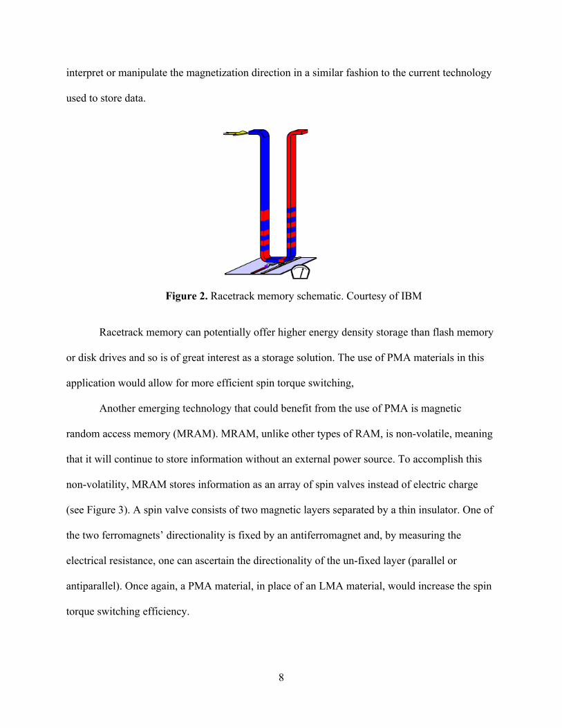
For example, racetrack memory, a novel way of storing data where a current is passed through a

wire, causing the domains therein to pass read and write heads. These stationary heads would

 

8

interpret or manipulate the magnetization direction in a similar fashion to the current technology

used to store data.

Figure 2. Racetrack memory schematic. Courtesy of IBM

 

Racetrack memory can potentially offer higher energy density storage than flash memory

or disk drives and so is of great interest as a storage solution. The use of PMA materials in this

application would allow for more efficient spin torque switching,

Another emerging technology that could benefit from the use of PMA is magnetic

random access memory (MRAM). MRAM, unlike other types of RAM, is non-volatile, meaning

that it will continue to store information without an external power source. To accomplish this

non-volatility, MRAM stores information as an array of spin valves instead of electric charge

(see Figure 3). A spin valve consists of two magnetic layers separated by a thin insulator. One of

the two ferromagnets’ directionality is fixed by an antiferromagnet and, by measuring the

electrical resistance, one can ascertain the directionality of the un-fixed layer (parallel or

antiparallel). Once again, a PMA material, in place of an LMA material, would increase the spin

torque switching efficiency.

 

9

Figure 3. Magnetic random access memory spin valve. Courtesy of the National University of Singapore

These technologies (both of which offer improvements on current memory technologies)

can be improved with the inclusion of PMA materials. By looking at the compositional and

magnetic properties of CoCrPt as well as the magnetic, topographical, and crystallographic

effects of varying the thickness of both the CoCrPt film and the Ti underlayer, a better

understanding of how the magnetic properties change under various conditions.

MAGNETIC  ANISOTROPY  

Because the directionality of a magnetic moment is dependent on several factors, the

anisotropy can be thought of as a balancing act between different properties/characteristics of the

material. In the case of thin-film CoCrPt, the main contributions to anisotropy come from the

shape of the material (thin film) and the crystalline anisotropy (hexagonal close packed crystal

structure).

Shape anisotropy occurs because the magnetic moments preferentially align to minimize

the amount of stray fields created by free poles on the surface of the magnet. These free poles in

turn create a demagnetizing field, defined as:

 

10

𝐻! = −𝑁𝑀 (1)

Where N is the demagnetizing factor and is dependent on the shape of the material and M is the

magnetization and is usually expressed (along with N, Hd) as a tensor. For a thin film (ignoring

edge effects), the demagnetizing factor can be simplified as:

𝑁 =0 0 00 0 00 0 1

(2)

and consequently the energy of the stray fields (Estr) due to the shape will be:

𝐸!"# = 12 𝜇!𝑀

! cos! 𝜃 (3)

Which gives a minimum energy of stray fields occurring at θ = 90º, indicating that an in-plane

magnetization would be favorable.

Crystal structure also defines easy and hard axes within a material. An easy or hard axis

is used to describe the natural alignment of the magnetic moment due to the position of the

atoms. The equilibrium direction of a magnetic moment will point in the direction that minimizes

the energy. For example, in some body-centered cubic (bcc) materials (like iron), it takes a

significantly smaller applied field to magnetize the material along the <100> directions (an easy

axis) than along the hardest directions, <111> (a hard axis). If there is no magnetic field present,

the magnetic moment will be aligned in the easy direction. Similar phenomenon can be seen in

materials with a hexagonal close packed (hcp) crystal structure. For example, in cobalt, the easy

axis is along the [0001], [0001] directions with a large field required to magnetize the material

along hard axis, the basal plane, defined as the other <1000> directions. In cobalt, as is shown in

Figure 4, saturation magnetization for the hard axis, [1000], exceeds 8000 Oe while the easy axis

saturates at a much lower field.

 

11

Figure 4. Crystallographic and magnetic properties of cobalt. (a) Hexagonal close packed crystal structure of cobalt with annotated easy and hard axis; (b) reaction of the magnetization of cobalt to an applied field along the hard and easy axis. Courtesy of Modern Magnetic Materials.1 Cobalt, and other materials that have a single preferential direction as their easy axis, are

often referred to as uniaxial materials. The energy associated with aligning along that easy axis is

defined as uniaxial crystal anisotropy energy density, which is usually expressed as a power

series, though it is usually simplified to the first three terms as follows:

𝑢! = 𝐾!! + 𝐾!! sin! 𝜃 + 𝐾!! sin! 𝜃 (4)

Because Ku0 is independent of direction, it is not helpful in understanding the anisotropy

of a sample. Values for the uniaxial crystal anisotropy energy density of cobalt are reported as

Ku1 = 4.1 x 106 erg/cc and Ku2 = 1.5 x 106 erg/cc1. A positive Ku1 indicates a favorable z-axis

orientation, as would be expected given the hexagonal packing of cobalt.

So, although shape anisotropy would dictate that thin films of CoCrPt should have an in-

plane magnetization, perpendicular magnetic anisotropy (PMA) can be achieved if the

magnetocrystalline anisotropy is greater than the shape determined anisotropy. By seeding the

appropriate orientation of the hexagonal close packed structure of CoCrPt, an out-of-plane

magnetization should dominate despite contributions from the shape.

When interfaces are present, magnetoelastic anisotropy can also affect the final

directionality and magnitude of the magnetic moment. In multilayer systems, mismatch between

the lattice constants and therefore the size of the unit cells will introduce strain into the lattice

 

12

itself. This strain distorts the unit cell thereby changing the crystallographic and magnetic

properties. For example, in a cubic system with several easy axes, applied strain can create a

uniaxial system.1

PERPENDICULAR  MAGNETIC  ANISOTROPY  

Perpendicular magnetic anisotropy (PMA) is a thin-film phenomenon where the shape

anisotropy of the thin film is overcome, resulting in a magnetization out of the plane of the film.

Shape anisotropy can be overcome by a strong crystalline anisotropy (Co alloys) or by interfaces

(Co/Pt multilayers, ordered FePt intermetallic). A high PMA value is useful and sought after

because it allows for higher density recording as well as increased efficiency in spin torque

switching.

PMA has units of energy density, usually J/cm3 or erg/cc. Values of PMA vary between

samples and are dependent on fabrication methods as well as treatment after fabrication.

However some reported values are 6.9 x 105, 3.2 x 105 erg/cc2 for CoCr films, 3.4 x 106 erg/cc

for CoCrPt films on an Cr-Ti underlayer3, and 3.7 x 106 erg/cc for Co73Cr15Pt12.4

As was mentioned before, a perpendicular magnetic moment requires a strong

magnetocrystalline anisotropy to overcome the shape anisotropy. This can be optimized in

several ways. First, the relative compositions of the elements can be tuned to maximize the out-

of-plane magnetization. Second, post-deposition annealing can be used to facilitate

homogenization of the films. Third, an underlayer can be added to facilitate the growth of the

correct phase and crystallographic orientation of the material.

Perpendicular alignment of magnetic moments is a useful characteristic for recording

high-density information. Perpendicular mediums can have a higher areal density of bits than

longitudinal medium (magnetized in the plane of the film) because the tendency towards

 

13

demagnetization is lower as it is stabilized against superparamagnetism.1 Therefore, a

perpendicular medium is of interest for increasing the bit-density for data storage.

COBALT  CHROMIUM  PLATINUM  THIN  FILMS  

Cobalt, as was mentioned above, has a hexagonal close packed (hcp) lattice structure,

leading to a magnetocrystalline anisotropy aligned on the z-axis. The energy density (see

Equation 4) of cobalt is approximately Ku1 = 4.1 x 106 emu/cc at room temperature.1 The lattice

constants for cobalt are a = b = 2.5071 Å and c = 4.0695 Å.5 However, these characteristics can

be manipulated by alloying cobalt with other elements, allowing it to be engineered for memory

storage applications.

The use of a magnetic film in memory storage devices (i.e. hard disk drives, MRAM,

racetrack memory) poses an interesting engineering problem because the materials used must

meet a specific set of requirements. First, out-of-plane alignment of the magnetic moments

(perpendicular magnetic anisotropy, PMA) is required to maximize the areal density of the

information storage as well as stabilize it against demagnetization due to superparamagnetism;

second, an ideal storage material has a large enough coercivity so that it is not in danger of self

demagnetizing; third, it must be able to withstand extreme environments; and fourth it must have

a relatively high signal to noise ratio for an easily measurable difference between the two logic

states.1

CoCrPt, with a PMA of approximately 8 x 106 erg/cc6, is an excellent candidate for

ultrahigh density magnetic recording material because it has a strong magnetocrystalline

anisotropy that can overcome the shape anisotropy of the thin film geometry7, it has good

thermal stability8,9, and displays very high corrosion resistance.10 CoCrPt can be engineered to

optimize its functionality as a storage device.

 

14

Cobalt naturally forms a hexagonal close packed structure. As discussed above, the

magnetocrystalline anisotropy of this system leads to preferential moment alignment along the z-

axis. This crystalline structure is also present in Co-Pt, Co-Cr, and CoCrPt alloys.4.

CoPt, a candidate for PMA materials, has excellent properties. The addition of Pt to the

cobalt lattice results in a small decrease in magnetization saturation4 and the coercivity of the

system is approximately 4300 Oe. It has a curie temperature of about 550 ºC and good corrosion

resistance. However, the coercivity is too high for it to be used with current memory storage

systems that have a limit of approximately 3000 Oe.1 CoCr also exhibits perpendicular magnetic

anisotropy. The addition of Cr to Co results in a segregation of Cr in the grain boundaries of the

system. This segregation results in an increased coercivity for the system as well as a decreased

saturation magnetization due to the uncoupling of the grains. However, the degree of segregation

is dependent on the deposition conditions, notably temperature. The addition of other elements to

Co-Cr systems has been shown to change various characteristics. Elements explored as additions

to CoCr films include Pt, Nb, Ta, Zr, V, Mo, Mn, Pd, B, and Re.11–15 However, platinum has

been shown to result in the best overall properties of the films—resulting in the greatest increase

in anisotropy and lowest decrease in magnetization saturization. The addition of 12-18% Pt,

while decreasing the saturation magnetization slightly (by about 100 emu/cc), increases the

anisotropy field from about 5 to 9 kOe.11 CoCrPt, of varying compositions, therefore, offers an

optimization of the properties present in Co-Cr and Co-Pt alloys. And, while Cr segregates to the

grain boundaries, Pt is soluble into the hcp cobalt lattice, resulting in a small change in lattice

parameter compared to that of a pure cobalt lattice.16 This change is dependent on the relative

composition of the Pt, but some reported values include a = b = 2.55-2.57Å for Pt = 10 at-%17

 

15

and c = 4.272 Å for Pt = 23 at-%16. Notably, the addition of Pt increases the perpendicular

component of the system.

Underlayers can be used to control the crystallographic orientation of the magnetic film

as well as the characteristics of the grains (including size, shape, and separation).18 Specifically,

in CoCrPt, the underlayer is used to induce epitaxial growth with a hcp (0002) orientation

perpendicular to the film. Underlayers reported include Ti (50 nm)19, CrTi15 (50, 100nm)8, Cr

(150 nm)20, Ag (20 nm)21, NiAl (100 nm)18, and Ta-Ru (10nm).17 Ti naturally inspires the (0001)

hcp texture in CoCrPt and has been shown to reduce the c-axis dispersion, leading to better

properties.19 There is a small lattice mismatch between Ti (a = 2.95 Å)19 and CoCrPt (as above, a

= 2.55-2.57), which introduce strain into the film at the interface between the two films. Despite

this, Ti is an excellent candidate as an underlayer for CoCrPt PMA thin films.

Some studies have been done on the effects of using a Ti underlayer in a CoCrPt system.

Sonobe, Ikada, Uchida, and Toyooka investigated the effects of a 25nm Ti underlayer on

Co72Cr28 film (sputtered at 200 ºC) focusing on the read/write characteristics of Co-Cr.22 Lee et

al. looked at how a CoZr seed layer affected the PMA properties of CoCr16.9Pt10.8/Ti (sputtered at

240 ºC) with a focus on minimizing the thickness of the Ti layer without losing the out-of-plane

magnetization.23 Gong et al. also studied Ti as an underlayer but with an Ag seed layer for

Co68Cr20Pt12 (sputtered at 250 ºC) to reduce c-axis dispersion and increase out-of-plane

magnetization of the sample.19 Sun et al. performed a series of investigations on CoCrPt/Ti/NiP

with NiP serving as a seed layer. Sputtering of Ti and Co74Cr16Pt10 was performed at 300 ºC.24–27

But, no work has been done for room temperature sputtering of Ti underlayers and CoCrPt films

without a seed layer. This project seeks to provide insight into the relationship between the

thickness of the Ti underlayer and the characteristics of CoCrPt film. Additionally, the effect of

 

16

the thickness of the CoCrPt layer on the properties of the system will also be addressed.

Furthermore, these results could engender studies involving the growth of PMA materials on

multiferroic substrates (specifically BiFeO3). CoCrPt is an excellent candidate for memory

storage applications and its optimization will lead to the enabling of new technologies.

OBJECTIVES  

1. Calculate the composition and Curie temperature of sputtered CoCrPt

2. Investigate the effects of changing the Ti underlayer thickness on the magnetic

properties, crystallographic texture, and topography of CoCrPt thin films

3. Investigate the effects of varying the thickness of CoCrPt magnetic films on the

magnetic properties, crystallographic texture, and topography of CoCrPt thin films with

a constant thickness underlayer

EXPERIMENTAL  DESIGN  AND  METHODS  

Various samples were created in order to investigate the inherent properties of CoCrPt as

well as to understand how varying certain parameters leads to a change in the magnetic,

topographical and crystallographic characteristics of the material.

SAMPLE  PREPARATION  

The CoCrPt and Ti thin films were deposited at room temperature on a naturally oxidized

silicon substrate (approximately 1 cm x 1 cm) by DC magnetron sputtering. Co66Cr22Pt12 and Ti

targets were bombarded with argon atoms, resulting in a thin film deposition on the substrate. All

depositions for CoCrPt occurred at 2.1-2.3 mTorr; all depositions for Ti occurred at 8.0-8.1

mTorr. All samples were rotated at a rate of 30 min-1.

 

17

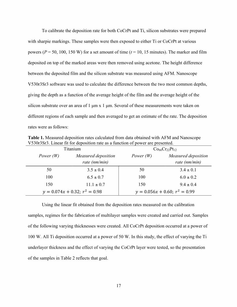
To calibrate the deposition rate for both CoCrPt and Ti, silicon substrates were prepared

with sharpie markings. These samples were then exposed to either Ti or CoCrPt at various

powers (P = 50, 100, 150 W) for a set amount of time (t = 10, 15 minutes). The marker and film

deposited on top of the marked areas were then removed using acetone. The height difference

between the deposited film and the silicon substrate was measured using AFM. Nanoscope

V530r3Sr3 software was used to calculate the difference between the two most common depths,

giving the depth as a function of the average height of the film and the average height of the

silicon substrate over an area of 1 µm x 1 µm. Several of these measurements were taken on

different regions of each sample and then averaged to get an estimate of the rate. The deposition

rates were as follows:

Table 1. Measured deposition rates calculated from data obtained with AFM and Nanoscope V530r3Sr3. Linear fit for deposition rate as a function of power are presented.

Titanium Co66Cr22Pt12 Power (W) Measured deposition

rate (nm/min) Power (W) Measured deposition

rate (nm/min) 50 3.5 ± 0.4 50 3.4 ± 0.1 100 6.5 ± 0.7 100 6.0 ± 0.2 150 11.1 ± 0.7 150 9.4 ± 0.4 𝑦 = 0.074𝑥 + 0.32;  𝑟! = 0.98 𝑦 = 0.056𝑥 + 0.60;  𝑟! = 0.99

Using the linear fit obtained from the deposition rates measured on the calibration

samples, regimes for the fabrication of multilayer samples were created and carried out. Samples

of the following varying thicknesses were created. All CoCrPt deposition occurred at a power of

100 W. All Ti deposition occurred at a power of 50 W. In this study, the effect of varying the Ti

underlayer thickness and the effect of varying the CoCrPt layer were tested, so the presentation

of the samples in Table 2 reflects that goal.

 

18

Table 2. Samples prepared using dc magnetron sputtering. Varying Ti thickness Varying CoCrPt thickness

Ti thickness (nm) CoCrPt thickness (nm) Ti thickness (nm) CoCrPt thickness

(nm) 20 90 80 50 40 90 80 75 60 90 80 100 70 90 80 125 80 90 80 150 90 90 100 90

These samples were tested to investigate their magnetic, topographical, and

crystallographic characteristics. The associated error for all samples created is due to the

uncertainty of the total volume of the film. The error for deposition can be summarized as ± 5nm

and the Si substrate size error can be assumed to be less than 0.04 cm2 for each sample.

SAMPLE  ANALYSIS  

As was described above in the Experimental Design, several characteristic techniques

were used to investigate the properties of the samples created (see Table 2).

ENERGY-­‐DISPERSIVE  X-­‐RAY  SPECTROMETER  

Energy-dispersive x-ray spectroscopy (EDS or EDX), usually coupled with a scanning

electron microscope (SEM), can be used to investigate the composition of a sample. EDS uses an

electron beam to excite the material; when the incident electron causes the dislodging of an inner

electron, an electron from one of the outer orbitals will fall to a lower energy state to replace it.

This change in energy level releases an x-ray with a wavelength characteristic to the elemental

identity of the atom. The x-rays emitted from a sample are detected and used to identify the

overall elemental composition of the sample. In general, the results are given as a set of peaks,

 

19

with the axes being energy (usually units of keV) versus intensity (usually units of cts or au). By

comparing the area under these peaks, the relative composition can be calculated.

All EDS results were obtained using a JEOL 6610LV SEM with Iridium Ultra EDS

software used for calculations of composition. All samples were cleaned using compressed air

and mounted on standard SEM stubs to ensure a level testing surface. All results were taken in

high vacuum. At least three measurements were taken from different regions of the sample.

VIBRATING  SAMPLE  MAGNETOMETER    

A vibrating sample magnetometer creates a uniform magnetic field in which a sample is

vibrated. Coils, placed near the sample, pick up the voltage induced by the moving sample (see

Figure 5). This voltage is proportional to the magnetic moment of the sample at that applied

field.

Figure 5. Schematic of a vibrating sample magnetometer. Courtesy of Wikipedia.

In a standard experiment, the field is set at -10,000 Oe and is incrementally changed until

it reaches 10,000 Oe. The regime is then reversed and measurements are taken as the field

decreases back to it’s original value. The hysteresis loops obtained from this measurement can be

 

20

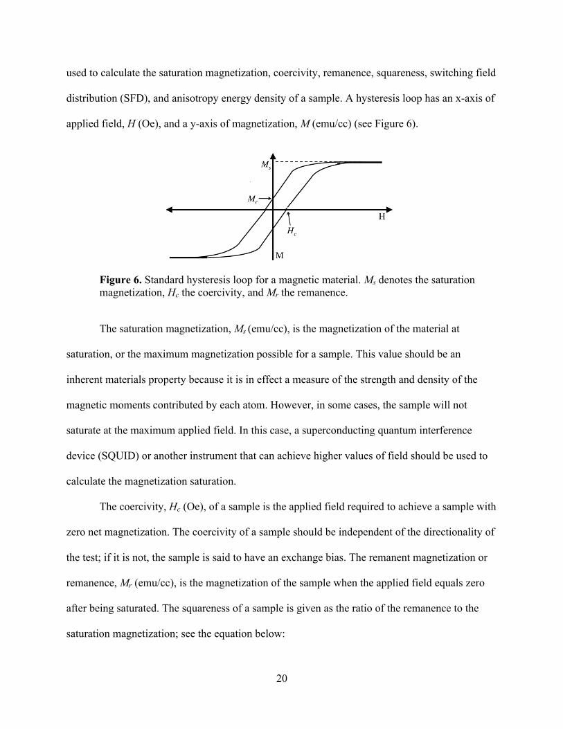
used to calculate the saturation magnetization, coercivity, remanence, squareness, switching field

distribution (SFD), and anisotropy energy density of a sample. A hysteresis loop has an x-axis of

applied field, H (Oe), and a y-axis of magnetization, M (emu/cc) (see Figure 6).

Figure 6. Standard hysteresis loop for a magnetic material. Ms denotes the saturation magnetization, Hc the coercivity, and Mr the remanence.

 

The saturation magnetization, Ms (emu/cc), is the magnetization of the material at

saturation, or the maximum magnetization possible for a sample. This value should be an

inherent materials property because it is in effect a measure of the strength and density of the

magnetic moments contributed by each atom. However, in some cases, the sample will not

saturate at the maximum applied field. In this case, a superconducting quantum interference

device (SQUID) or another instrument that can achieve higher values of field should be used to

calculate the magnetization saturation.

The coercivity, Hc (Oe), of a sample is the applied field required to achieve a sample with

zero net magnetization. The coercivity of a sample should be independent of the directionality of

the test; if it is not, the sample is said to have an exchange bias. The remanent magnetization or

remanence, Mr (emu/cc), is the magnetization of the sample when the applied field equals zero

after being saturated. The squareness of a sample is given as the ratio of the remanence to the

saturation magnetization; see the equation below:

 

21

𝑆 =𝑀!

𝑀! (5)

Squareness is useful as a comparative tool and is a representation of the strength of the readable

signal in the absence of a field (H = 0). A higher squareness is desirable for recording media.

The anisotropy energy density, Ku1 is discussed theoretically above. Experimentally, the

value Ku1 can be calculated as either

𝐾!! =12𝑀!𝐻! (6)

Where Ms is the saturation magnetization of the easy axis loop and Hk is the anisotropy field,

equal to the field where the easy axis and hard axis loops intercept. This method for calculating

the anisotropy energy density is flawed because, for hard axis loops (in this case, in-plane), the

corrected data often is approximated to have a magnetization saturation that is lower than that of

the easy axis. Because this data has been corrected, the anisotropy field (Hk) is difficult to

approximate. Another method (and the method that will be used in this project) for finding the

value of the anisotropy energy density is to find the difference in area between the easy and hard

axis loops in the first quadrant of a standard hysteresis loop (H > 0; M > 0).1 Because it is a

measure of the difference in the amount of energy it would take to align the magnetization along

the easy axis versus the hard axis, a high anisotropy energy density is desirable to prevent

demagnetization and to increase thermal stability.

The switching field distribution (SFD) can be calculated by finding the full width, half

maximum (FWHM) of the Gaussian fit of the derivative of the M-H curve plotted against the

applied field (H) values. In this project, the form of the Gaussian fit was as follows:

𝑓 𝑥 = 𝑎  exp   −𝑥 − 𝑏𝑐

!

(7)

 

22

The SFD is a measure of the size distribution of particles, with a high SFD correlating to more

homogenous distribution of sizes. For use in magnetic storage, regular grains are desirable as

irregular grain shapes lead to noise when reading the data.

The Curie temperature can also be found by taking measurements at different

temperatures. The Curie temperature is defined as the temperature at which the saturation

magnetization approaches zero and the hysteresis loops show a paramagnetic response.

The VSM used for all experiments presented here was a DMS Model 1600 Signal

Processor, Model 32KG Gaussmeter, Model 883A Temperature Controller as well as

MicroSense VSM. The data was recorded using the MicroSense EasyVSM program.

For each sample, the recipe for the VSM was as follows (ΔH indicates step size): ΔH =

500 Oe for H = [-10000, -2000], ΔH = 200 Oe for H = [-2000, 2000], ΔH = 500 Oe for H =

[2000, 10000] where H is the applied field (units Oe) and the recipe is repeated in the opposite

direction as well (10000 to -10000 Oe).

To test the Curie temperature, samples were held at temperature (T = 150, 250, 300, 350,

400, 450, 500, 600 ºC) for 15 minutes, then the testing as described above was completed and the

sample was cooled to room temperature before another test was performed.

One major source of error in the calculating the aforementioned values (saturation

magnetization, coercivity, etc.) is the uncertainty in calculating the total volume of the sample

since the results are reported in emu/cc instead of emu, as is recorded by the instrument. Any

errors in thickness, or in the measurements of the dimensions for the samples will be carried

forward and will affect the final values presented. Additionally, the step size of the

measurements can account for some of the error, with large step sizes resulting in more

uncertainty.

 

23

X-­‐RAY  DIFFRACTOMETER  

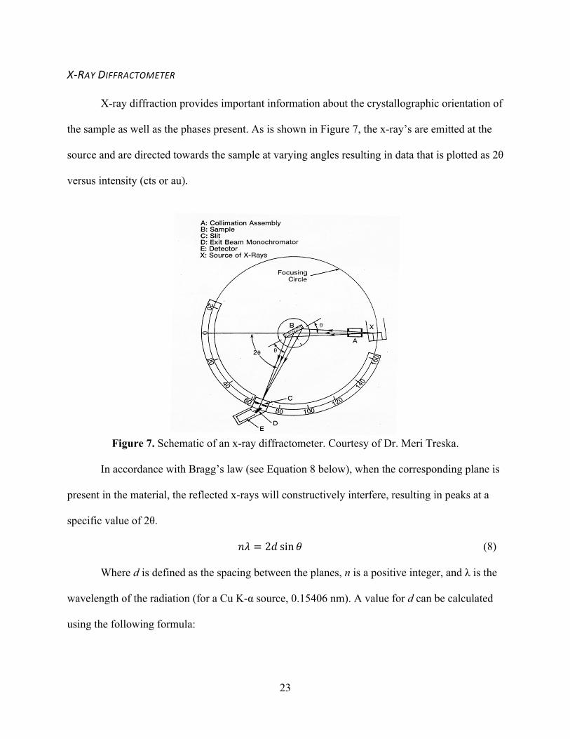
X-ray diffraction provides important information about the crystallographic orientation of

the sample as well as the phases present. As is shown in Figure 7, the x-ray’s are emitted at the

source and are directed towards the sample at varying angles resulting in data that is plotted as 2θ

versus intensity (cts or au).

Figure 7. Schematic of an x-ray diffractometer. Courtesy of Dr. Meri Treska.

In accordance with Bragg’s law (see Equation 8 below), when the corresponding plane is

present in the material, the reflected x-rays will constructively interfere, resulting in peaks at a

specific value of 2θ.

𝑛𝜆 = 2𝑑 sin𝜃 (8)

Where d is defined as the spacing between the planes, n is a positive integer, and λ is the

wavelength of the radiation (for a Cu K-α source, 0.15406 nm). A value for d can be calculated

using the following formula:

 

24

𝑑 =𝑎

ℎ! + 𝑘! + 𝑙! (9)

where a is equal to the lattice constant associated with the plane and h, k, and l are the miller

indices of the incident plane (hkl).

Though the intensity (cts) of these peaks cannot be compared between results of different

samples, intensities of peaks within the same run of a sample can be compared. For example, a

comparison between the intensity of the (0001) peak and the intensity of the (1010) peak of an

hcp material would result in a comparative intensity factor, m, as below:

𝑚 =𝐼(!!!")𝐼(!"!!)

(10)

This factor gives an idea of the alignment of the crystal and which planes are aligned to

better interact with the radiation source. In hcp CoCrPt, a strong (0001) peak is desirable.

All samples were crystallographically investigated using a PANalytical X’Pert PRO

XRPD. No additional preparation of samples was performed. The scans were run from 2θ = 20º -

80º with a scan step size of 0.0167º. Peaks were identified and matched using the X’Pert

Highscore software database.

ATOMIC  FORCE  MICROSCOPE  

Atomic force microscopy can be used to investigate the topography of a surface. A

cantilever with a pyramidal point at the tip is linearly tapped along the surface of the material.

This is done repeatedly to create an image of the surface of the sample. Changes in the response

of the cantilever are measured by the reflection of a laser that is centered, at rest, on the tip of the

cantilever. An atomic form microscope (AFM) allows the user to calculate the depth of an edge,

the roughness of a sample, and several other functionalities. However, atomic force microscopy

 

25

gives no information on the composition of the film itself and requires a specific magnetic tip to

analyze magnetic domain size and structure.

All results presented were obtained with a Dimension 3100 Atomic Force Microscope

(Nanscope IV SPM Control Station, Veeco) and were processed using Nanoscope V530r3Sr3

software. The sample size for each reading was 1.0 µm by 1.0 µm and the maximum scan speed

for the tip was 4.0 µm/sec. At least three regions of each sample were tested and the values

presented are the averages of these three regions.

RESULTS  AND  DISCUSSION  

This project will be divided into three sections to best discuss the results of this study.

The first is the composition and magnetic properties of CoCrPt, which will present the data

concerning the measured composition of the samples, and the curie temperature of the CoCrPt

films used in this report. Second, the effects of changing the thickness of the Ti underlayer will

be discussed with respect to the topographical roughness, the crystallography, and the magnetic

properties: saturation magnetization, coercivity, remanence, squareness, SFD, and anisotropy

energy density. The same characterization studies were undertaken to understand the effect of

varying the thickness of the CoCrPt magnetic layer.

COMPOSITION  AND  MAGNETIC  PROPERTIES  OF  COCRPT  

Several investigations were carried out to better understand the properties of the CoCrPt

alloy fabricated. Results for both composition and Curie temperature are presented below.

COMPOSITION  

 

26

The composition of the sputtered CoCrPt thin films was investigated with EDS. All

samples tested had an underlayer of 80 nm Ti. The averaged composition from these samples

was Co60.2Cr16.4Pt23.4 (subscripts represent atomic percent measured) and the results from each

sample are presented in Table 3 below:

Table 3. Composition (at-%) of CoCrPt thin films created by sputtering off a Co66Cr22Pt12 target. Compositions shown are an average of at least 5 measurements at different points on the sample; error reported is the maximum standard deviation of the data for each sample

Sample Thickness (nm) Composition Error

75 Co60.2Cr16.2Pt23.6 ± 1.0%

100 Co59.3Cr16.1Pt24.6 ± 0.7%

125 Co60.2Cr16.5Pt23.3 ± 0.4%

150 Co61.1Cr16.7Pt22.2 ± 0.5%

This measured composition differs from the reported value on the target used,

(Co66Cr22Pt12) though the reported composition is very consistent between samples of different

thicknesses.

This inconsistency is probably due to different sputtering rates of elements. Because each

constituent has a different sputtering rate, it is difficult to maintain the same stoichiometry in the

sputtered film as is found in the multicomponent target. Because several scans were done at

many different points of the samples, it is unlikely that the films are macroscopically (area > 50

µm) heterogeneous. This composition has implications for the characteristics discussed below

because amount of platinum added to the Co-Cr system has been shown to affect the properties

of the system.

Because Pt is known to increase the stacking fault density in CoCrPt28, a larger

percentage of Pt could disrupt homogenous uniaxial grain growth. These stacking faults would

 

27

lead to a weaker PMA material. In direct competition with this effect is the effect that the

addition of Pt has on the magnetocrystalline anisotropy and magnetostriction. Liu et al. reported

that for (Co90Cr10)1-xPtx on a CrW underlayer an increase from x = 8.5 at-% to 25 at-% results in

an increase in both magnetocrystalline and magnetoelastic anisotropy. These increases generally

lead to an increase in coercivity and are caused by the changes in the lattice parameters of the

CoCrPt samples (a = 2.537 to 2.617 Å; c = 4.141 to 4.272 Å) and the resultant change in the

mismatch between the CoCrPt and the underlayer.16 So, though the high concentration of Pt

could potentially interrupt the crystallographic structure of the film, it also results in a

comparatively larger magnetocrystalline anisotropy than would be expected in a film with a

lower concentration of Pt.

It is also possible that this high percentage of Pt could have promoted uniaxial growth of

PMA CoCrPt. A 90nm film of CoCrPt on bare naturally oxidized Silicon had the hysteresis loop

shown in Figure 8.

 

28

Figure 8. In-plane and out-of-plane hysteresis loops for Co60.2Cr16.4Pt23.4 (t = 90nm) on bare, naturally oxidized Si. Circles (○) indicate out-of-plane directionality of testing; upward facing triangles ( ) indicate in-plane directionality for testing. Lines connect points.

The in-plane hysteresis loop appears to represent the hard axis of the material, requiring a

large field to saturate. The out-of plane hysteresis loop, on the other hand saturates relatively

quickly, indicating an easy axis.

Because there is clear difference in the shape of the curves, there is anisotropy present in

this material. In comparison with the easy and hard axis M-H curves in Figure 4, it follows that

the out-of-plane magnetization is more energetically favorable than the in-plane magnetization

(which is still not saturated at 10,000 Oe). Ergo, the CoCrPt film seems to behave like a PMA

material even without an underlayer present.

CURIE  TEMPERATURE  

-10000 -5000 0 5000 10000

-300

-200

-100

0

100

200

300

Mag

netic

mom

ent (

emu/

cc)

Field (Oe)

 

29

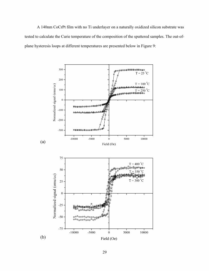
A 140nm CoCrPt film with no Ti underlayer on a naturally oxidized silicon substrate was

tested to calculate the Curie temperature of the composition of the sputtered samples. The out-of-

plane hysteresis loops at different temperatures are presented below in Figure 9:

 

30

Figure 9. Out-of plane M-H curves for CoCrPt thin films (t = 140nm) at different temperatures, as labeled in images. For clarity, only three loops are shown for each graph; parentheses indicate the symbol used. (a) shows T = 25(□), 100( ), 250(○) ºC; (b) shows T = 300 (□), 350( ), 400(○) ºC; (c) shows T = 450(□), 500( ), 600(○) ºC. Lines connect points.

The trends in magnetization saturation, coercivity, remanence, and squareness of the

temperature dependent out-of-plane hysteresis loops are reported below in Figure 9:

 

31

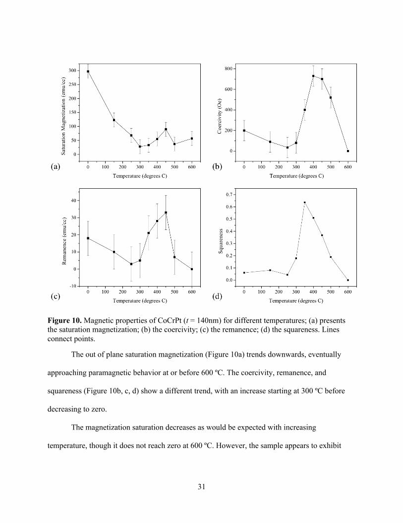
Figure 10. Magnetic properties of CoCrPt (t = 140nm) for different temperatures; (a) presents the saturation magnetization; (b) the coercivity; (c) the remanence; (d) the squareness. Lines connect points.

The out of plane saturation magnetization (Figure 10a) trends downwards, eventually

approaching paramagnetic behavior at or before 600 ºC. The coercivity, remanence, and

squareness (Figure 10b, c, d) show a different trend, with an increase starting at 300 ºC before

decreasing to zero.

The magnetization saturation decreases as would be expected with increasing

temperature, though it does not reach zero at 600 ºC. However, the sample appears to exhibit

 

32

parametric behavior when tested at 600ºC because it has an approximately linear slope (see

Figure 9).

Though, when the field is at its maximum value (H = 10,000 Oe), the magnetization

value is approximately 57 Oe, not zero as one might expect. However, there is no visible

hysteresis and the sample appears to be behaving paramagnetically.

The increasing then decreasing trend, displayed in coercivity, remanence, and squareness

is potentially due to some annealing that occurred while the sample was held at temperature,

allowing it to reorder into a structure that has better PMA characteristics. This effect was studied

by Sun et al. who annealed their Co74Cr16Pt10 (t < 40nm) at 550 ºC for 10 minutes in a vacuum

furnace and reported an increase of approximately 1000 Oe in coercivity when measured at room

temperature following the treatment.27

Another process that could be occurring is the preferential oxidization of Cr. Because Cr

is the most easily oxidized in the CoCrPt sample, the amount of Cr available to participate in the

magnetic properties of the sample is lower than that reported in the composition.2 If the Cr is

able to segregate in the grain boundaries, the resulting less chromium in the grain boundaries due

to oxidation could explain the trends observed in coercivity, remanenece, and squareness in

Figure 10.

To confirm that a physical change occurred in the samples, one sample, held at 500 ºC for

approximately 40 minutes was tested at room temperature and compared to the out-of-loop

hysteresis loop with no annealing in Figure 11:

 

33

Figure 11. Out-of loop hysteresis loops for CoCrPt (t = 140nm) films with no post-fabrication treatment (circle ○) and annealing at 500ºC for approximately 40 minutes (upward facing triangle ). Lines connect points.

There is a notable decrease in magnetization saturation, from approximately 265 emu/cc

without post fabrication processing to 100 emu/cc with the 500 ºC anneal. There is also an

increase in coercivity, from 165 Oe with no annealing to 795 Oe.

These changes in magnetic properties are likely due to the segregation of Cr to the grain

boundaries along with, potentially, the oxidation of this Cr. Additionally, the change in magnetic

properties in Figure 11 show that in the process of measuring the Curie temperature, the films’

properties change.

 

-10000 0 10000

-300

-200

-100

0

100

200

300

Nor

mal

ized

sign

al (e

mu/

cc)

Field (Oe)

 

34

EFFECTS  OF  VARYING  TI  UNDERLAYER  THICKNESS    

The thickness of the Ti underlayer (t = 20, 40, 60, 70, 80, 90, 100) has a large effect on

many of the properties of thin-film CoCrPt. For clarification, the results have been separated into

three sections: magnetic properties, crystallography, and topography.

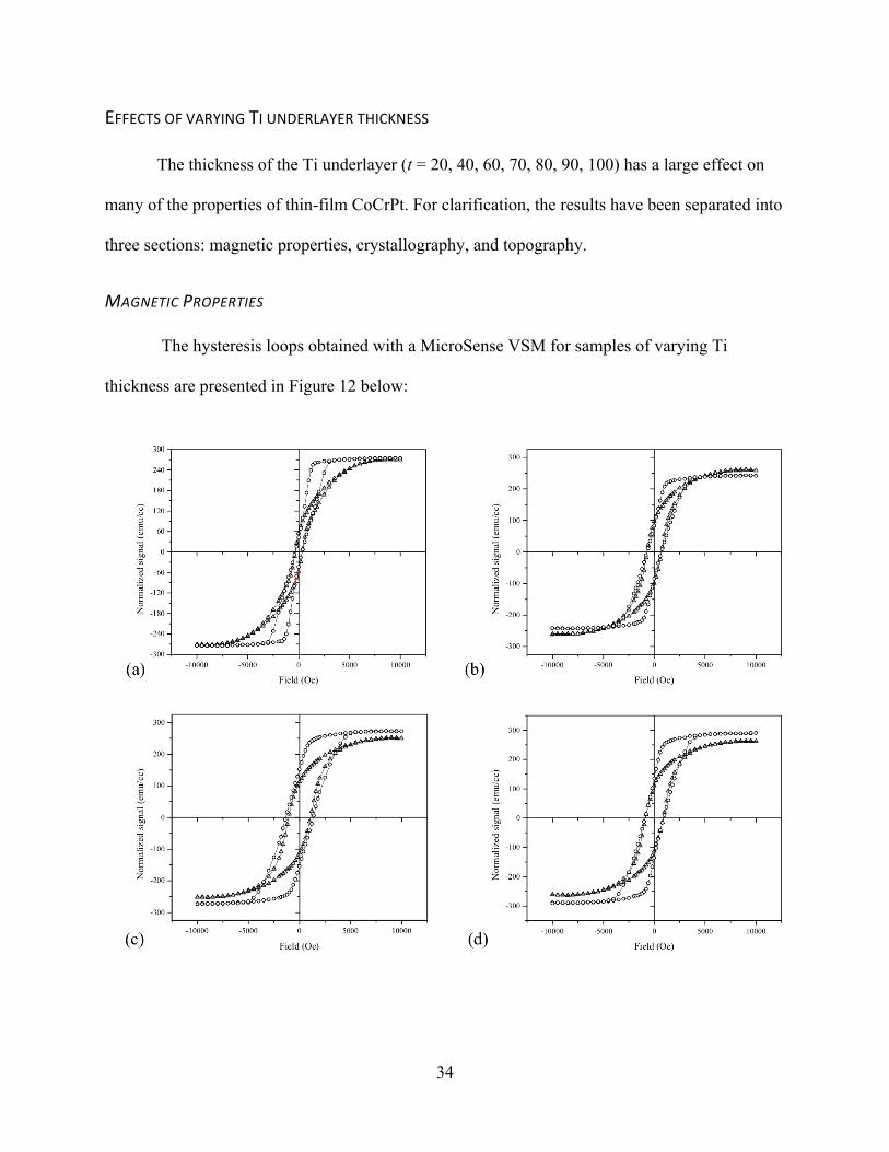
MAGNETIC  PROPERTIES  

The hysteresis loops obtained with a MicroSense VSM for samples of varying Ti

thickness are presented in Figure 12 below:

 

35

Figure 12. M-H curves for CoCrPt thin films (t = 90nm) with varying Ti underlayer thickness. In each graph, a circle (○) indicates out-of-plane loops and an upward facing triangle ( ) indicates the in-plane loops. Underlayer thickness values are as follows (a) t = 20nm; (b) t = 40nm; (c) t = 60nm; (d) t = 70nm; (e) t = 80nm; (f) t = 90nm; (g) t = 100nm. Lines connect points.

The magnetic properties, specifically the magnetization saturation, coercivity, remanence,

squareness, switching field distribution, and anisotropy energy density, were calculated and are

presented in Figure 13 as a function of Ti underlayer thickness.

 

36

Figure 13. The out-of-plane magnetic properties of CoCrPt (t = 90nm) and variable Ti underlayer thickness (t = 20, 40, 60, 70, 80, 90, 100nm). The properties are as follows (a)

 

37

magnetization saturation (emu/cc), (b) coercivity (Oe), (c) remanence (emu/cc), (d) squareness, (e) switching field distribution (Oe), (f) anisotropy energy density (erg/cc). Lines connect points.

The saturation magnetization (Figure 13a), though changing slightly, does not show a

dramatic dependence on the thickness of the underlayer. The greatest difference is a 20%

decrease between t = 0 and t = 40nm. The coercivity (Figure 13b) steadily increases until it

seems to stabilize above 60nm Ti at about 1200 Oe. The remanence (Figure 13c) follows a

similar trend as the coercivity, showing initial increase that eventually levels off at or above

60nm Ti with a difference of about 400% between t = 20nm and t = 60nm. The shape of the

squareness (Figure 13d, calculated using Equation 5) also follows the trend seen in the

remanence and coercivity, with a 500% increase between t = 20nm and t = 60nm.

The anisotropy (Figure 13e) shows an increase, then a decrease in a trend very similar to

those described above for coercivity, remanence, and squareness. There is an approximately

300% difference between the lowest value (at t = 40nm) and the highest value (at t = 80nm)

reported. However, the switching field distribution (Figure 13f), much like the saturation

magnetization, does not show a clear trend with changing underlayer. The greatest difference is

between a Ti thickness of t = 40nm and t = 80nm, which shows an approximately 20% decrease.

The differences between values for magnetization saturation (i.e. between Ms of t = 0 and

t = 40nm) can be explained by possible errors in calculations of volume of the film present. In

general, since the composition of the material does not appear to differ greatly between samples

(Table 3), the saturation magnetization should be constant, which seems to be confirmed by the

data presented in Figure 13a.

The increase in coercivity as Ti thickness increases implies that at around 60nm, the

texture of the Ti is sufficient to nucleate substantial (0002) growth in the CoCrPt film. This

increased grain growth and organization would lead to a higher coercivity because columnar

 

38

grains forming in the c-axis direction, (0002), would allow for a macroscopic out-of-plane

orientation of magnetic moments. The growth of columnar grains requires a certain threshold

thickness, which according to the data in Figure 13b is at approximately t = 60nm. This columnar

grain growth, along with the fact that chromium (with an at-% lower than 18) segregates at the

grain boundaries, isolating the grains and allowing for a greater coercivity1, explains why there is

an observable increase in coercivity

The increase in remanence is similarly motivated because the factors that increase

coercivity should also increase the remanent magnetization (at zero applied field). An increase in

remanence means that there is a stronger preference for an out-of-plane easy axis orientation of

the magnetization. The uniaxial growth of hcp CoCrPt due to columnar grains of Ti increases the

favorability of magnetization to point out-of-plane. The trend in the squareness, very similar to

both the trend in remanence and the coercivity, is dominated by the remanence (found in the

denominator of Equation 5) since there is no dramatic change in magnetization saturation as Ti

thickness changes.

The anisotropy, which shows a similar trend to coercivity, remanence, and squareness, is

also a reflection of how strongly aligned out of plane the magnetization. As a measurement of

the difference in the amount of energy it would take to align the magnetic moment along the easy

and hard axis, the increase in anisotropy energy density can be understood as an indication that it

is more favorable for the moments to align perpendicular to the plane (c-axis).

Any differences SFD between the different thicknesses can be explained first by errors in

calculating the volume of the sample and secondly by the inaccuracy of the Gaussian fits

(Equation 7) used to calculate the SFD. The fits used to calculate the values presented in Figure

13f are given below in Table 4.

 

39

Table 4. Gaussian fits used to calculate the switching field distribution of samples with varying Ti underlayer thicknesses. See Equation 7. Ti underlayer thickness (nm) A b c R2 value

20 0.15 217.7 2076 0.84

40 0.13 557.8 2002 0.92

60 0.13 1279 2382 0.96

70 0.15 808.4 1974 0.93

80 0.12 1595 2626 0.96

90 0.15 907.2 2015 0.94

100 0.14 942.5 2028 0.94

Most of the R2 values are greater than 0.90, indicating a fairly good fit for the data.

However, some of the variation in the reported SFD (full width half maximum value) could be

explained by this factor.

CRYSTALLOGRAPHY  

The texture of the samples was interrogated using a PANalytical X’Pert PRO XRPD X-

ray diffractometer. Figure 14 presents the superimposed data from several samples with different

underlayer thickness.

 

40

Figure 14. XRD scans for 90nm CoCrPt films with varying Ti underlayer thickness (t = 20, 40, 60, 70, 80, 90, 100nm). Peaks identified using X’Pert Highscore software databases.

The peaks present in any of the samples presented are labeled in the above figure. The

identification of these peaks was achieved with X’Pert Highscore software. All samples showed

evidence of the (0002) plane, though with increasing underlayer thickness, the (0002) peaks shift

left. All substrate and titanium peaks do not appear to shift with changing underlayer thickness.

All CoCrPt samples indicate the presence of the (0002) plane. Other planes that are

present include (0110) at t = 20nm and (0111) at t = 70, 90, 100nm though the intensity of these

peaks is very low compared to the (0002) plane. Both planes never achieve more than 10% of the

intensity of the c-axis (0002) plane. The (1120) plane has a strong presence in the samples where

25 30 35 40 45 50 55 60 65 70 75 800

2500

5000

7500

10000

12500

15000

Ti = 100nmTi = 90nm

Ti = 80nm

Ti = 70nmTi = 60nmTi = 40nm

Inte

nsity

(au)

2θ

Ti = 20nm

32.8

o Si s

ubst

rate

41.1

o Co(

01-1

0)

43.8

o Co(

0002

)

46.6

o Co(

01-1

1)

56.5

o Ti(0

2-21

)

61.7

o Si s

ubst

rate

74.8

o Co(

11-2

0)

69.2

o Si s

ubst

rate

66.2

o Ti(0

002)

 

41

t = 60 and 70nm. Table 5 presents the relevant information for the (0002) peak identities for all

samples.

Table 5. Crystallographic values acquired with XRD scans (step size 0.0167º) for varying Ti underlayer thickness (t = 20, 40, 60, 70, 80, 90, 100nm). Values calculated with X’Pert Highscore software.

Ti thickness (0002) peak location (2θ) d (Å) c (Å) FWHM

20 43.72 2.071 ± 0.002 4.142 ± 0.002 0.4512 ± 0.008

40 43.80 2.067 ± 0.002 4.134 ± 0.002 0.2342 ± 0.008

60 43.84 2.065 ± 0.002 4.130 ± 0.002 0.2342 ± 0.008

70 43.68 2.072 ± 0.002 4.144 ± 0.002 0.2342 ± 0.008

80 43.70 2.071 ± 0.002 4.142 ± 0.002 0.2342 ± 0.008

90 43.69 2.072 ± 0.002 4.144 ± 0.002 0.2342 ± 0.008

100 43.69 2.072 ± 0.002 4.144 ± 0.002 0.2007 ± 0.008

The shifting of the (0002) peak results to lower peak in a larger c lattice constant (see

Figure 4 [0001] easy axis for reference). The d value (calculated using Equation 8) is directly

dependent on the peak location and c; the lattice constant can be derived from the plane spacing,

d (see Equation 9). The full width, half maximum values remain constant except for t = 20nm

which features a much wider peak and t = 100nm which features a slightly skinnier peak.

Since the unit cell volume is kept constant, this increase in the c lattice constant would

lead to a decrease in the a lattice constant. This elongation of the lattice cell would theoretically

increase the magnetocrystalline energy, and so increase the anisotropy. This increase in

anisotropy energy density with increasing Ti thickness is supported by the data reported in

Figure 13e. This trend implies that better PMA materials are created at higher thickness of Ti

underlayer.

 

42

The FWHM values should give an insight into the c-axis dispersion, or how broad the

distribution of orientations of each moment is. Because the FWHM values are constant for most

of the values, it can be assumed that except for edge cases, the underlayer thickness does not

greatly affect the c-axis dispersion of a sample. However, as will be discussed in the Conclusion,

there are other methods to more accurately test this value that could help distinguish if there is

any change due to Ti underlayer thickness. However, at t = 20nm, the FWHM is nearly twice the

value of the other samples. This implies that the film was more disordered with less homogenous

uniaxial growth, probably because the Ti film was too thin to allow for sufficient influence on

the CoCrPt films.

TOPOGRAPHY    

The roughness of the samples shows a trend of increasing roughness as thickness of the

CoCrPt layer increases. As is shown in Figure 15, the 80nm Ti underlayer sample has an

approximately four times rougher surface than the sample with a 20nm underlayer.

 

43

Figure 15. Trend of roughness measured for samples with constant thickness CoCrPt layers (t = 90nm) and varying thickness Ti layers. Lines connect points.

This increasing roughness likely is due to an increase in grain size29. As the underlayer

thickness increases to a critical point (approximately t = 60nm), homogenous large grains are

formed. A rougher surface results in more free poles and pinning sites, leading to a more

complex domain structure. This new domain structure should result in increased coercivity

(observed in Figure 13b) and broader SFD peaks (not observed in Figure 13f). Since the SFD

values show no real trend, there is probably also a secondary reason for the increase in roughness

as CoCrPt increases.

EFFECTS  OF  VARYING  COCRPT  FILM  THICKNESS    

After choosing the sample with the greatest inherent coercivity (Ti underlayer t = 80nm),

several thicknesses of CoCrPt film (t = 50, 75, 90, 100, 125, 150) were fabricated and tested to

investigate how the magnetic, crystallographic and topographical characteristics of the system

20 40 60 80 1000.5

1.0

1.5

2.0

2.5

3.0

3.5

4.0

Rou

ghne

ss (n

m)

Thickness Ti (nm)

 

44

change. For clarification, the results have been separated into three sections: magnetic properties,

crystallography, and topography.

MAGNETIC  PROPERTIES  

The hysteresis loops obtained with a MicroSense VSM for samples of varying Ti

thickness are presented in Figure 16 below:

 

45

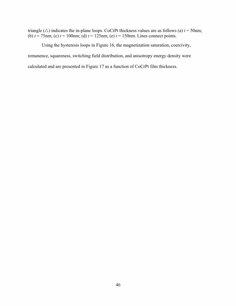
Figure 16. Out-of plane M-H curves for constant Ti underlayer (t = 80nm) with varying CoCrPt film thickness. In each graph, a circle (○) indicates out-of-plane loops and an upward facing

 

46

triangle ( ) indicates the in-plane loops. CoCrPt thickness values are as follows (a) t = 50nm; (b) t = 75nm; (c) t = 100nm; (d) t = 125nm; (e) t = 150nm. Lines connect points.

Using the hysteresis loops in Figure 16, the magnetization saturation, coercivity,

remanence, squareness, switching field distribution, and anisotropy energy density were

calculated and are presented in Figure 17 as a function of CoCrPt film thickness.

 

47

Figure 17. The out-of-plane magnetic properties of CoCrPt (t = 50, 75, 100, 125, 150nm) and constant Ti underlayer thickness (t = 80nm). The properties are as follows (a) magnetization

 

48

saturation (emu/cc), (b) coercivity (Oe), (c) remanence (emu/cc), (d) squareness, (e) anisotropy energy density (erg/cc); (f) switching field distribution (Oe). Lines connect points.

The out-of-plane magnetization saturation (Figure 17a) seems to show a slight downward

trend, with a 25% decrease between t = 50nm and t = 150nm. The coercivity (Figure 17b) of the

sample has a similar downwards trend, decreasing by a total of approximately 350 Oe. The

remanence (Figure 17c) has a similar downward trend, decreasing from about 200 emu/cc to 80

emu/cc as the thickness of the CoCrPt film increases.

The squareness (Figure 17d) follows the trend of gradually decreasing as thickness of

CoCrPt increases. The maximum value reported is 0.67 for t = 50nm with minimum values

reported as 0.35 and 0.36 for t = 125nm and t = 150nm. The maximum values are nearly twice

the minimum values. The anisotropy energy density (Figure 17e) seems to remain fairly

constant. Though there is some fluctuation, the changes in values are minimal considering the

inherent error and the small magnitude of the differences. The SFD (Figure 17f) shows a unique

trend; it increases by about 1000 Oe total as the CoCrPt film thickness increases.

The slight downward trend in the magnetization saturation with increasing CoCrPt

thickness is probably mostly due to errors in the estimation of the volume of the sample and step

sizes used to measure these values. As was discussed above, since the material composition is

constant, one would expect to see a consistent value for magnetization saturation. The coercivity

also generally decreases which would make sense because as the film thickens, the uniaxial

crystal organization is more likely to interrupted or shifted because of the method of fabrication,

sputtering. There is also possibly relaxation of the lattice, which would be strained at the Ti-

CoCrPt interface. The relaxation, which would be possible only in a sufficiently thick layer,

would result in a change in the lattice parameters, which would in turn affect the strength of the

magnetocrystalline anisotropy. Additionally, the rotation of moments is easier in a thicker film.

 

49

In a thin film, the rotation of magnetic moments incurs an energy penalty because it creates free

poles on the surface. In a thicker film, this becomes easier, resulting in a decreased coercivity

and remanence (see Figure 17b, c).

The remanence also shows a trend of decreasing as the film thickness increases. This is

similarly explained by the increasing likelihood that the film will be less ordered as it gets

thicker. A less perfectly ordered film would show a lower magnetization in the c-axis direction

(out-of-plane) at a zero field. Likewise, a relaxation in the lattice as the thickness increases

would result in a decrease in remanence. The squareness, like in the case with the changing Ti

thickness, is dominated by the remanence since the magnetization saturation does change

significantly over the range of CoCrPt thicknesses.

The anisotropy energy density increases and decreases, but seems to have a notable

decrease of about one third of the maximum value. Again, this could be explained by a relaxation

in the lattice leading to a decrease in the difference between the energy needed to align the

magnetization on the easy or hard axis. The switching field distribution shows a steady increase,

which implies that the homogeneity of the size of particles is increasing with increasing CoCrPt

film thickness. The Gaussian fits used to describe data for varying CoCrPt thickness is presented

below in Table 6.

 

50

Table 6. Gaussian fits used to calculate the switching field distribution of samples with varying CoCrPt film thicknesses. See Equation 7.

CoCrPt film thickness (nm) a b c R2 value

50 0.18 1122 1697 0.97

75 0.15 912.8 1877 0.95

100 0.16 770.9 2148 0.93

125 0.14 650.4 2229 0.92

150 0.12 652.9 2316 0.96

The majority of these fits have R2 ≥ 0.95, indicating that a Gaussian is a good predictor

for the behavior of the data. However, there is still some error inherent in the data presented

because the fit is not a perfect match for the data.

CRYSTALLOGRAPHY  

The texture of the samples was interrogated using a PANalytical X’Pert PRO XRPD X-

ray diffractometer. Figure 18 presents the superimposed data from several samples with different

CoCrPt film thickness.

 

51

Figure 18. XRD scans for varying thickness CoCrPt films (t = 50, 75, 90, 100, 125, 150nm) and an 80nm Ti underlayer. Peaks identified using X’Pert Highscore software databases.

The labeled peaks in Figure 18 are present in at least one of the samples. The

identification of these peaks was achieved with X’Pert Highscore software. The cobalt (0002)

peaks appear to shift left as CoCrPt film thickness increases. The substrate peaks and the

titanium peak do not appear to shift significantly.

The (0002) plane is present in all samples with variable CoCrPt peaks. The (11-20) plane

only appears in the sample with a CoCrPt thickness of t = 50nm. The (01-11) plane also only

appears in one sample (t = 150nm). The (01-10) peak appears in samples with thickness of t =

75, 100, and 150nm. Table 7 presents the relevant information for the (0002) peak identities for

all samples.

20 25 30 35 40 45 50 55 60 65 70 75 800

2000

4000

6000

8000

10000

12000

CoCrPt = 150nm

69.2

o Si s

ubst

rate61.7

o Si s

ubst

rate

32.8

o Si s

ubst

rate

56.5

o Ti(0

2-21

)

66.2

o Ti(0

002)

74.8

o Co(

11-2

0)

46.6

o Co(

01-1

1)

41.1

o Co(

01-1

0)

43.8

o Co(

0002

)

CoCrPt = 125nm

CoCrPt = 100nm

CoCrPt = 90nm

CoCrPt = 75nm

Inte

nsity

(cts

)

2θ

CoCrPt = 50nm

 

52

Table 7. Crystallographic values acquired with XRD scans (step size 0.0167º) for varying CoCrPt underlayer thickness (t = 50, 75, 100, 125, 150nm). Values calculated with X’Pert Highscore software.

CoCrPt film thickness

(0002) peak location (2θ) d (Å) c (Å) FWHM

50 43.64 2.074 ± 0.002 4.148 ± 0.002 0.1338 ± 0.008

75 43.68 2.072 ± 0.002 4.144 ± 0.002 0.2676 ± 0.008

100 43.65 2.073 ± 0.002 4.146 ± 0.002 0.2342 ± 0.008

125 43.66 2.073 ± 0.002 4.146 ± 0.002 0.2342 ± 0.008

150 42.61 2.075 ± 0.002 4.150 ± 0.002 0.2342 ± 0.008

With increasing thickness of the CoCrPt film, the (0002) peak generally shifts to lower

values of 2θ. This trend is mirrored in the increase of d (calculated with Equation 8) and the

increase of the lattice constant c. The values for FWHM are constant for t = 100, 125 and 150nm.

When t = 50nm, the FWHM is much lower than would be expected and when t = 75nm, the

FWHM has a slightly higher value than was observed for the other thicknesses.

This shifting of the peaks leads to, as was discussed above in the changing Ti thickness

section, an increase in lattice constant (c) is expected. This increasing lattice constant should lead

to a more elongated unit cell with a larger magnetocrystalline anisotropy than a unit cell with a

shorter c lattice constant. Surprisingly, Figure 17e indicates a slight decrease in anisotropy with

increasing thickness, implying that there are other factors that affect the anisotropy energy

density beyond simply lattice constant.

The FWHM constant values for t > 100nm implies that there is no change in the c-axis

dispersion of the samples. However, as will be discussed in the Conclusion, there are other

methods to more accurately test this value that could help distinguish if there is any change due

to CoCrPt film thickness. At t = 50nm, the FWHM has a lower value than the other samples,

 

53

implying that there is less c-axis dispersion for this film thickness. At t = 75nm, the opposite is

true, with a FWHM value that would imply a greater amount of c-axis dispersion than the other

samples. Because these values do not support a trend with a clear motivation, these abnormalities

are probably due to errors in the software calculation or lack of resolution on the peaks. Again,

another method might be better suited to make a definitive statement about how the c-axis

dispersion changes with the thickness of the CoCrPt film.

TOPOGRAPHY  

With the Ti underlayer kept constant (t = 80nm), the thickness of the CoCrPt film may

have an effect on the roughness of the sputtered film. The measured roughness of the films is

presented in Figure 19.

Figure 19. Trend of roughness measured for samples with varying thickness CoCrPt layers and constant thickness Ti layers (t = 80nm). Lines connect points.

50 75 100 125 1502.0

2.5

3.0

3.5

4.0

Rou

ghne

ss (n

m)

Thickness CoCrPt (nm)

 

54

As CoCrPt increases, the roughness of the samples appears to increase and then decrease.

However, because the difference in the values is approximately within the bounds of the error

due to the nature of the measurement, the roughness could be assumed to remain roughly

constant with increasing film thickness. This implies that t = 50nm is thick enough to have

overcome any inhomogeneity due to the sputtering of a very thin layer.

CONCLUSION  AND  FURTHER  WORK  

CoCrPt has many potential applications in memory storage because of its perpendicular

magnetic anisotropy. The encouragement of this specific property through growth is often

dependent on an underlayer to ensure hcp c-axis growth. This project investigated the inherent

properties of the CoCrPt film fabricated, the effect of changing the thickness of a Ti underlayer,

and the effect of changing the thickness of the CoCrPt magnetic film.

The composition of the fabricated samples was found to be Co60.2Cr16.4Pt23.4, very

different than the expected Co66Cr22Pt12 given for the target. The increased platinum content

could possibly explain why even CoCrPt film without an underlayer exhibited some PMA

behavior. The Curie temperature of Co60.2Cr16.4Pt23.4 is approximately 600 ºC where the out-of-

plane hysteresis loop has obvious paramagnetic trends.

The addition of a Ti underlayer affects certain magnetic properties of CoCrPt (t = 90nm).

As the thickness of the Ti increases to a critical value (t ≥ 60nm), the coercivity also increases,

reaching a maximum of about 1250 Oe. The remanence follows a similar trend, increasing to a

maximum value of about 155 emu/cc. The anisotropy also seems to follow this trend, though the

plateau above t = 60nm is less obvious. All of these patterns are likely caused by the widespread

nucleation of c-axis oriented columnar grains in the Ti underlayer. Both the magnetization

 

55

saturation and switching field distribution do not show a dependence on the thickness of the

underlayer.

The XRD scans do not show a drastic change in the lattice parameter of the cobalt lattice

as a function of the Ti underlayer and the fairly constant FWHM values imply an unchanging c-

axis dispersion, though this could be studied in more detail. A notable exception is the t = 20

sample, which had a much wider FWHM, implying that that thickness of underlayer is perhaps

insufficient to inspire homogenous out-of-plane growth. The topography of the CoCrPt film

changes greatly with underlayer thickness—the roughness of the sample increases with

increasing Ti underlayer, appearing to plateau, again, at t = 60nm. This increase is probably due

to the formation of smaller grains, a theory supported by the similarly shaped increase in

coercivity.

Studies were also completed with a fixed Ti underlayer thickness (t = 80nm) with

variable thicknesses of CoCrPt magnetic films. The coercivity and remanence trend downward

as CoCrPt film thickens, which could imply the relaxation of the lattice as the distance between

the interface increases. The increase in the switching field distribution with increasing thickness

suggests that having a thicker film increases the homogeneity of the grains in the sample. The

anisotropy and magnetization saturation appear to be unaffected by alterations in the CoCrPt.

XRD scans show a trend of increasing lattice constant as the CoCrPt thickness increases,

supporting the hypothesis that some relaxation of the lattice occurs in the thicker films. The

roughness of the film stays fairly constant with increasing CoCrPt thickness.

In order to better understand the interactions between the Ti underlayer and the CoCrPt

film, there are several more characterization methods that could be employed. As was mentioned

above, a better study of the x-ray diffraction patterns could reveal important information.

 

56

Rocking curves would give a more exact value for FWHM and the distribution of grain

orientation within the sample.

The films could also be cross-sectioned and observed with a TEM or SEM to try and

observe the columnar grains. The films could also be studied using a selected area electron

diffraction analysis on the TEM to ascertain how well aligned the CoCrPt crystal is in

comparison to the Ti underlayer.

Additional work that could be performed is the observation how varying Ti or CoCrPt

thickness affects the grain and domain size. The average grain size as well as the distribution of

grain sizes could be observed with a scanning electron microscope and similar information could

be obtained about the magnetic domains in the material using a magnetic force microscope. This

information would complement the data collected on the magnetic properties, crystallography,

and topography of CoCrPt with Ti underlayers.

   

 

57

WORKS  CITED  1 R.C. O’Handley, Modern Magnetic Materials: Principles and Applications (John Wiley & Sons, Inc., 2000).

2 C.W. Chen, J. Mater. Sci. 26, 3125 (1991).

3 N. Inaba, A. Nakamura, T. Yamamoto, Y. Hosoe, and M. Futamoto, J. Appl. Phys. 79, 5354 (1996).

4 M.L. Plumer, J. van Ek, and D. Weller, editors , The Physics of Ultra-High-Desnity Magnetic Recording (Springer, New York, 2001).

5 C.L. Yaws, Yaw’s Handbook of Properties of the Chemical Elements (Knovel, 2011).

6 H. Sato, T. Shimatsu, K. Mitsuzuka, T. OIkawa, O. Kitakami, S. Okamoto, H. Muraoka, H. Aoi, and Y. Nakamura, Nippon Oya Jiki Gakkaishi 29, 427 (2005).

7 M.-Y. Im, J.-R. Jeong, and S.-C. Shin, J. Magn. Magn. Mater. 286, 442 (2005).

8 M. Futamoto, Y. Hirayama, N. Inaba, Y. Honda, L. Ito, A. Kikuga, and T. Takeuchi, IEEE Trans. Magn. 35, 2802 (1999).

9 P. Glijer, J.M. Sivertsen, and J.H. Judy, J. Appl. Phys. 73, 5563 (1993).

10 C. Tsai, J. Liang, H.H. Liang, and C.M. Wang, J. Magn. Magn. Mater. 209, 157 (2000).

11 T. Keitoku, J. Ariake, N. Honda, K. Ouchi, and S. Iwasaki, J. Magn. Magn. Mater. 176, 25 (1997).

12 O. Kitakami, N. Kikuchi, S. Okamoto, Y. Shimada, K. Oikawa, Y. Otani, and K. Fukamichi, J. Magn. Magn. Mater. 202, 305 (1999).

13 M. Sago and T. Inoue, J. Appl. Phys. 67, 6394 (1990).

14 U.M. Gana, Int. J. Res. Rev. Appl. Sci. 17, 370 (2013).

15 H. Song, K.-H. Shin, and S.-J. Kwon, J. Magn. Magn. Mater. 226-230, 1666 (2001).

16 X. Liu, Z. Li, W. Shi, S. Li, F. Wei, D. Wei, and X. Liu, J. Appl. Phys. 105, 07D503 (2009).

17 C.L. Platt, K.W. Wierman, E.B. Svedberg, T.J. Klemmer, J.K. Howard, and D.J. Smith, J. Magn. Magn. Mater. 247, 153 (2002).

18 L. Tang, L. Lee, D.E. Laughlin, and D.N. Lambeth, Appl. Phys. Lett. 69, 1163 (1996).

 

58

19 H. Gong, M. Rao, D.E. Laughlin, and D.N. Lambeth, J. Appl. Phys. 85, 4699 (1999).

20 G. Choe, IEEE Trans. Magn. 31, 2809 (1995).

21 F. Gao, H. Sun, S. Feng, H. Yu, L. Jia, C. Pan, H. Zhou, X. Nie, and Y. Sun, Trans. Nonferrous Met. Soc. China 15, 400 (2005).

22 Y. Sonobe, Y. Ikeda, H. Uchida, and T. Toyooka, J. Appl. Phys. 81, 4667 (1997).

23 I.S. Lee, H. Ryu, H.J. Lee, and T.D. Lee, J. Appl. Phys. 85, 6133 (1999).

24 C.J. Sun, G.M. Chow, J.P. Wang, E.W. Soo, and J.H. Je, J. Appl. Phys. 93, 8725 (2003).

25 C.J. Sun, G.M. Chow, E.W. Soo, J.P. Wang, Y.K. Hwu, T.S. Cho, J.H. Je, H.H. Lee, J.W. Kim, and D.Y. Noh, J. Nanosci. Nanotechnol. 1, 271 (2001).

26 C.J. Sun, G.M. Chow, J.P. Wang, E.W. Soo, Y.K. Hwu, J.H. Je, T.S. Cho, H.H. Lee, and D.Y. Noh, J. Appl. Phys. 91, 7182 (2002).

27 C.J. Sun, J.P. Wang, E.W. Soo, and G.M. Chow, J. Appl. Phys. 95, 7303 (2004).

28 P. Jang, S. Hong, and J. Kim, J. Appl. Phys. 93, 7741 (2003).

29 M.A. Parker, K.E. Johnson, C. Hwand, and A. Bermea, IEEE Trans. Magn. 27, 4730 (1991).

Picture Credit

Figure 1. http://hyperphysics.phy-astr.gsu.edu/hbase/audio/tape2.html

Figure 2. http://www.gitam.edu/eresource/Engg_Phys/semester_2/magnetic/magrecording.htm

Figure 3. http://www.ece.nus.edu.sg/isml/MRAM.jpg