kaleidoscope eyes: microstructure and optical performance
TRANSCRIPT
1
Kaleidoscope Eyes: Microstructure and Optical Performance of Chiton Ocelli Leanne Friedrich1, Wai Sze Lam2, Lyle Gordon1, Paul Smeets1, Robert Free1, Lesley Brooker3, Russell Chipman2,
and Derk Joester1* 1 Materials Science and Engineering, Northwestern University, Evanston, IL 60208. 2 College of Optical Sciences, University of Arizona, Tucson, AZ 85721. 3 GeneCology Research Centre, University of the Sunshine Coast, Sippy Downs, QLD 4556, Australia.
* to whom correspondence should be addressed: [email protected]
Keywords: chiton, aragonite, biomineralization, birefringence, twinning
Abstract
The chiton Acanthopleura granulata uses aragonitic lenses embedded in its shell to focus light onto photorecep-
tors. Because aragonite is biaxially birefringent, the microstructure of the lens greatly impacts the optical perfor-
mance. In addition, the chiton lives in the intertidal, so lenses experience two environments with different refrac-
tive indices: air and water. Using EBSD, we find that the lens is polycrystalline and contains curved grain bound-
aries. A combination of large, twinned grains and nanotwins ensure that the aragonitic ⟨001⟩ axis is consistent
across the lens. However, the orientation of the ⟨001⟩ axis relative to the shell varies between lenses. Ray tracing
simulations predict the optical performance of lenses of various microstructures in wet and dry environments.
Though twinning helps to limit birefringence-induced aberrations, variations in the orientation of the ⟨001⟩ axis
between lenses lead to variations in focal lengths between lenses and cause image doubling in some lenses. As
such, the birefringence of aragonite does not help the lens to transmit focused images in both air and water.
1 Introduction Across a broad range of phyla, biominerals are used to reinforce tissues.[1] Functional roles further include
homeostasis of essential ions such as Ca2+, acceleration and gravity sensing, and orientation in magnetic fields.[1,2]
Much less explored is the use of biominerals to manipulate light.[3–8] The extinct trilobites famously employed
single-crystalline calcite lenses in their compound eyes, and the extant brittlestar Ophiocoma wendtii uses similar
lenses for photoreception.[9–13] Both organisms evolved solutions to design problems that are general, such as the
creation of ellipsoid lens volumes or the correction of spherical aberration, but also to the specific problem of
double refraction of calcite. Double refraction is the consequence of birefringence, i.e. the dependence of the
refractive index on the polarization and direction of propagation of light, and leads to the well-known doubling of
images viewed through a calcite crystal.
While the choice of calcite as a material for lenses in an optical system may not be obvious, there are
numerous examples where large, intricately shaped, and smoothly curving skeletal elements are comprised of one
oriented single crystal of calcite and occluded macromolecules.[14] Creating the desired shape thus seems to be a
manageable problem. Furthermore, birefringence in calcite is uniaxial, meaning that the material is optically iso-
tropic for rays parallel to the axis of birefringence. With good control over non-equilibrium shape and lattice
orientation of large single crystals, there are some straightforward ways to optimize lens design. Not so for arag-
onite, a polymorph of calcium carbonate frequently used by marine biomineralizing organisms. Aragonite not only
displays biaxial birefringence, but also typically appears as a fine-grained polycrystalline material. Double refrac-
tion, scattering, and internal reflection at grain boundaries are expected to degrade the optical performance of
polycrystalline lenses. Nevertheless, some chitons are uniquely known to construct an optical system from arago-
nite,[15,16] begging the question how they may have overcome the limitations inherent in the material they use.
Chitons are a diverse group of marine mollusks of the class Polyplacophora that have a characteristic
dorsal shell comprised of eight plates or valves (Figure 1A). These valves are constructed from polycrystalline
aragonite. Each valve is riddled with branching sensory and secretory channels connecting the dorsal surface to
2
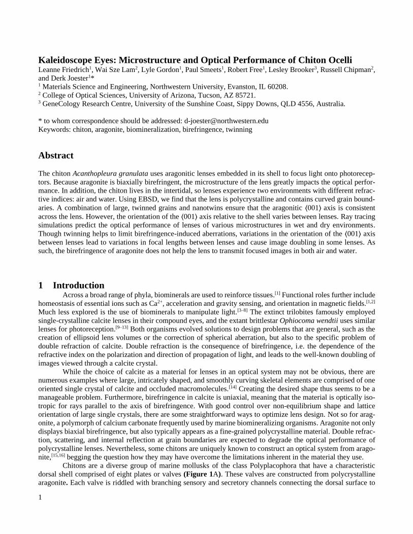
the mantle.[17] For eight genera of chitons, these channels terminate at the dorsal surface in light sensory organs
called ocelli (Figure 1B-D).[15] For example, in Acanthopleura granulata, the West Indian fuzzy chiton, ocelli are
composed of an aragonite lens suspended above the rhabdom, a 45-70 micron-deep cavity that contains roughly
180 sensory cells.[15,18] Lenses are biconvex and are covered by an aragonitic “cornea” (Figure 1C, D).[15,16,18] The
sensory cavity and lens are flanked by aragonite containing pheomelanin pigment (Figure 1D).[19]
Figure 1. A) Dorsal aspect of A. granulata. B) Reflected light image of dorsal surface of valve wetted by water. Ocelli are recognizable by
a ring of pigment (arrows). C) Reflected light image of cross-section of ocellus. Note that soft tissues have been removed and lens is partially
obscured by pigmented valve. D) Schematic drawing of ocellus cross section.
Behavioral studies suggest that A. granulata may be capable of spatial vision.[15] Speiser and coworkers
proposed that an aragonite lens may exhibit two focal lengths (for light of orthogonal polarization), thereby ena-
bling chitons to perceive their environment while submerged in water and when exposed to air.[15] To test this
hypothesis, a more detailed model of the lens is required. Herein, we investigate the microstructure of the A.
granulata ocellus lens and evaluate its impact on the optical performance of ocelli using a combination of experi-
ments and ray tracing simulations.
2 Results
2.1 Microstructure of the lens In electron backscatter diffraction (EBSD) maps of ground and polished sections, lenses can be distin-
guished from the surrounding valve and the cornea by a roughly elliptical dark (non-indexed) line that circum-
scribes the lens (Figure 2A-C). We found that the average lens diameter was d = 33 7.5 µm (N = 19), and the
maximum was d = 41 µm. Given the literature average of 55 2.3 µm,[16] it is likely that the majority of the
sections described herein did not contain the center of the lens.
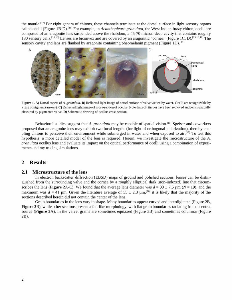
Grain boundaries in the lens vary in shape. Many boundaries appear curved and interdigitated (Figure 2B,
Figure 3B), while other sections present a fan-like morphology, with flat grain boundaries radiating from a central
source (Figure 3A). In the valve, grains are sometimes equiaxed (Figure 3B) and sometimes columnar (Figure
2B).
3
Figure 2. A, B) SEM-EBSD maps of embedded sections of lenses isolated from A. granulata. Orientation maps use an inverse pole figure
color scheme, where the color indicates the crystallographic axis parallel to surface normal of the section (see inset in B). Areas rendered
in black could not be indexed. Note curved, interdigitating grain boundaries (asterisks in B). C,D,E) Pole figures of the lens in (B). (E)
shows the aragonitic optic axis. F,G) Width of the distribution of ⟨001⟩ orientations, in geological aragonite (N = 4 maps), within the lens
(N = 18), and in the remainder of the valve (N = 1). The angular distribution was fit as a bivariate normal distribution along the long and
short axes designated by the Kent distribution, where widths were measured separately for each map. F) Widths averaged over all grains.
Inset: close-up of peak in (C), with long and short standard deviation annotated. G) Width averaged per grain. Grains are defined using a
critical misorientation of 1° and a critical size of 100 pixels.
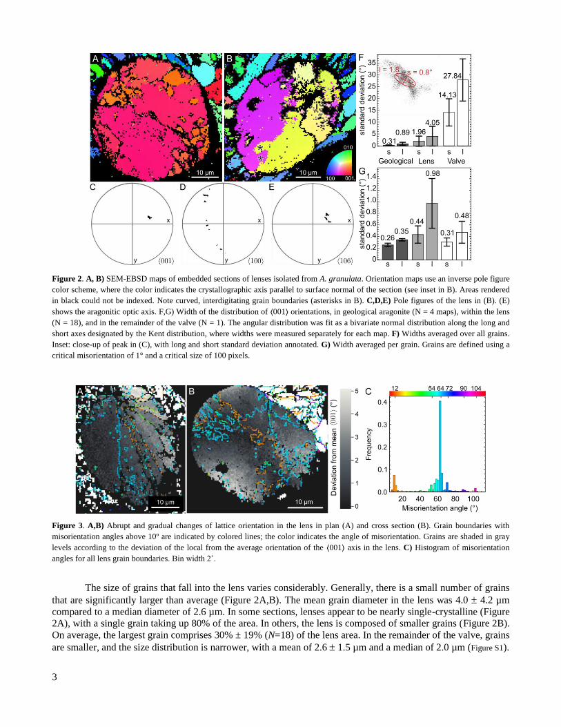
Figure 3. A,B) Abrupt and gradual changes of lattice orientation in the lens in plan (A) and cross section (B). Grain boundaries with
misorientation angles above 10º are indicated by colored lines; the color indicates the angle of misorientation. Grains are shaded in gray
levels according to the deviation of the local from the average orientation of the ⟨001⟩ axis in the lens. C) Histogram of misorientation
angles for all lens grain boundaries. Bin width 2˚.
The size of grains that fall into the lens varies considerably. Generally, there is a small number of grains
that are significantly larger than average (Figure 2A,B). The mean grain diameter in the lens was 4.0 4.2 µm
compared to a median diameter of 2.6 µm. In some sections, lenses appear to be nearly single-crystalline (Figure
2A), with a single grain taking up 80% of the area. In others, the lens is composed of smaller grains (Figure 2B).
On average, the largest grain comprises 30% ± 19% (N=18) of the lens area. In the remainder of the valve, grains
are smaller, and the size distribution is narrower, with a mean of 2.6 1.5 µm and a median of 2.0 µm (Figure S1).

4
2.2 Crystallographic texture EBSD pole figures show dramatic differences in texture between the lens and the valve (Figure 2, Table
S3, Table S4, Table S6, Table S5). In the lens, ⟨001⟩ axes are tightly aligned (Figure 2C,F). In contrast, ⟨100⟩ axes
and the optic axis (approximately the ⟨106⟩) trace narrow arcs, indicating that only the ⟨001⟩ axis is aligned (Figure
2D,E). In the valve, the ⟨100⟩ and ⟨001⟩ axes both trace diffuse arcs, indicating that the valve microstructure has
limited texture (Figure S4, Figure 2F). The orientation distribution of the ⟨001⟩ axis is seven times narrower in the
lens than in the valve, but both regions still have wider ⟨001⟩ axis distributions than geological crystals (Figure
2F). Due to difficulties in preserving the cornea during sample preparation, we have relatively little information
on its crystallographic texture (Figure S4). While ⟨001⟩ axes in the lens are highly aligned, we find that for any
given lens, the angle between the optical axis of the lens and the mean ⟨001⟩ axis falls into the interval α = 21º -
82º, seemingly at random.
In the lens, the orientation of the ⟨001⟩ axis changes gradually within individual grains (Figure 3B). Within
individual grains, ⟨001⟩ axis distributions are wider in lens grains than in grains in the surrounding valve, likely
because lens grains are larger (Figure 2G). ⟨001⟩ axis distributions in the small grains in the valve are the same
size as distributions in the much larger grains of geological crystals (Figure 2G).
The axis and angle of misorientation, i.e. the parameters of a rotation that superposes the two lattices,
describe orientation relationships between neighboring grains. The probability distribution of the misorientation
angles exhibits a sharp global maximum at 64˚ (Figure 3C). The angle between the mean axis of misorientation of
this type of grain boundary and the ⟨001⟩ axis is very small (0.06˚), indicating that the ⟨001⟩ axis remains static
across the grain boundary (Figure S2). Grain boundaries with a misorientation angle of 64˚ and misorientation axis
of ⟨001⟩, are consistent with aragonitic twin boundaries on the {110} plane, although planar twinning on the {110} plane is not apparent at the microscale (Figure 3A,B). For local maxima at 12˚ and 54˚, the angle between the
mean axis of misorientation and the ⟨001⟩ axis is also rather small (≤ 1.6˚). However, this angle is large enough
to enable small changes in ⟨001⟩ axis orientation at 12˚ and 54˚ grain boundaries to accumulate into large changes
in ⟨001⟩ axis orientation across the lens (Figure 3A). The axes of rotation for all other local maxima in the miso-
rientation angle probability distribution do not appear to be aligned.
2.3 Nano-twinning In addition to microscopic twinning, aragonite is known to display nano-twinning.[20–23] TEM imaging
using bright field (BF) contrast indicates that nanotwins with a characteristic size of 10-100 nm are present in the
lens of A. granulata (Figure 4). Nanotwins can be found within grains and at the interfaces between grains (Figure
4A) and have coherent (110) interfaces (Figure 4B,C). Within the nanotwin, spot doubling is apparent in fast
Fourier transforms of the lattice. Superposition of matrix and twin plane reflections produces spot doubling.[21]
Figure 4. A) Bright field TEM image of nanotwins (nt) at the interface between two grains (g1, g2). B) HRTEM image of a nanotwin on
the [1̅12] zone axis. Matrix (M) and twin (T) planes are annotated. C) Fast Fourier transform of (B), showing spot doubling (arrows)
which is indicative of twinning.
5
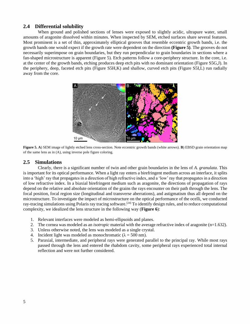
2.4 Differential solubility When ground and polished sections of lenses were exposed to slightly acidic, ultrapure water, small
amounts of aragonite dissolved within minutes. When inspected by SEM, etched surfaces share several features.
Most prominent is a set of thin, approximately elliptical grooves that resemble eccentric growth bands, i.e. the
growth bands one would expect if the growth rate were dependent on the direction (Figure 5). The grooves do not
necessarily superimpose on grain boundaries, but they run perpendicular to grain boundaries in sections where a
fan-shaped microstructure is apparent (Figure 5). Etch patterns follow a core-periphery structure. In the core, i.e.
at the center of the growth bands, etching produces deep etch pits with no dominant orientation (Figure S5G,J). In
the periphery, deep, faceted etch pits (Figure S5H,K) and shallow, curved etch pits (Figure S5I,L) run radially
away from the core.
Figure 5. A) SEM image of lightly etched lens cross-section. Note eccentric growth bands (white arrows). B) EBSD grain orientation map
of the same lens as in (A), using inverse pole figure coloring.
2.5 Simulations Clearly, there is a significant number of twin and other grain boundaries in the lens of A. granulata. This
is important for its optical performance. When a light ray enters a birefringent medium across an interface, it splits
into a ‘high’ ray that propagates in a direction of high refractive index, and a ‘low’ ray that propagates in a direction
of low refractive index. In a biaxial birefringent medium such as aragonite, the directions of propagation of rays
depend on the relative and absolute orientation of the grains the rays encounter on their path through the lens. The
focal position, focal region size (longitudinal and transverse aberrations), and astigmatism thus all depend on the
microstructure. To investigate the impact of microstructure on the optical performance of the ocelli, we conducted
ray-tracing simulations using Polaris ray tracing software.[24] To identify design rules, and to reduce computational
complexity, we idealized the lens structure in the following way (Figure 6):
1. Relevant interfaces were modeled as hemi-ellipsoids and planes.
2. The cornea was modeled as an isotropic material with the average refractive index of aragonite (n=1.632).
3. Unless otherwise noted, the lens was modeled as a single crystal.
4. Incident light was modeled as monochromatic (λ = 500 nm).
5. Paraxial, intermediate, and peripheral rays were generated parallel to the principal ray. While most rays
passed through the lens and entered the rhabdom cavity, some peripheral rays experienced total internal
reflection and were not further considered.
6
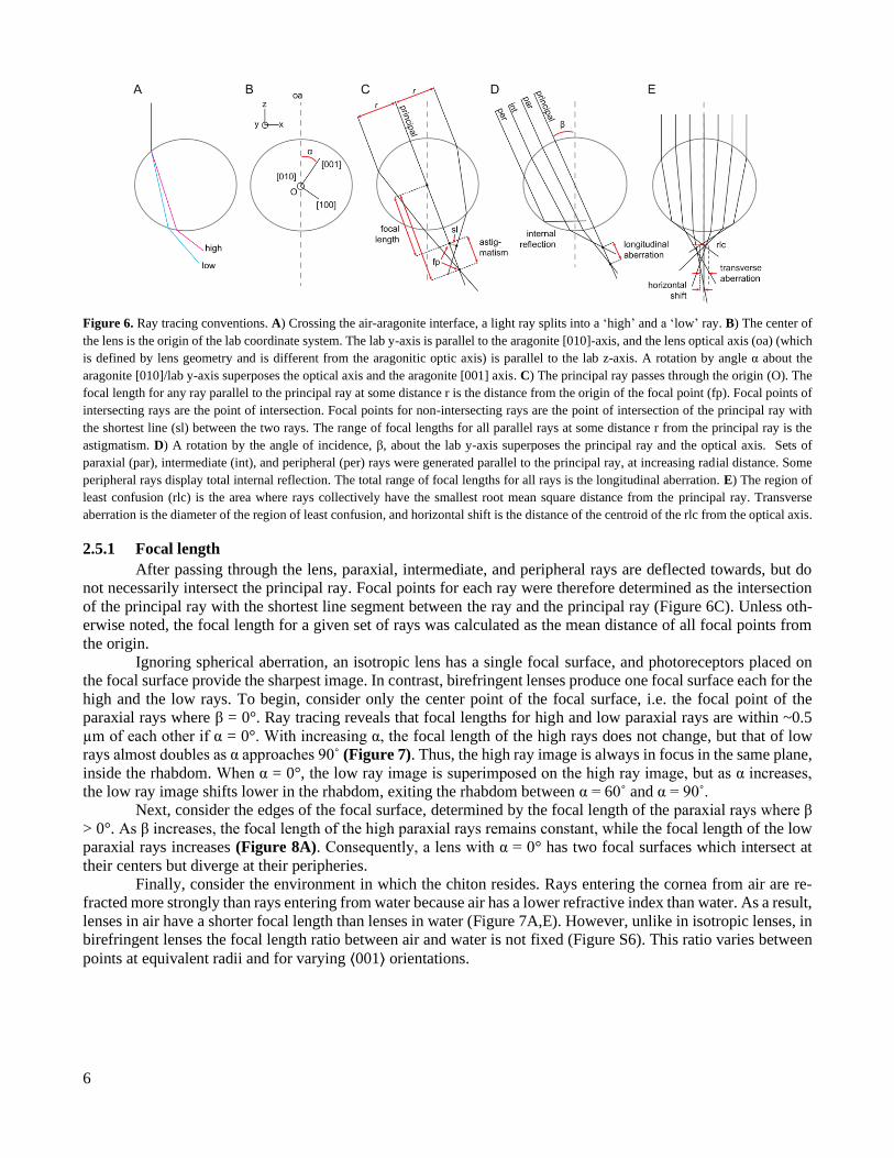
Figure 6. Ray tracing conventions. A) Crossing the air-aragonite interface, a light ray splits into a ‘high’ and a ‘low’ ray. B) The center of
the lens is the origin of the lab coordinate system. The lab y-axis is parallel to the aragonite [010]-axis, and the lens optical axis (oa) (which
is defined by lens geometry and is different from the aragonitic optic axis) is parallel to the lab z-axis. A rotation by angle α about the
aragonite [010]/lab y-axis superposes the optical axis and the aragonite [001] axis. C) The principal ray passes through the origin (O). The
focal length for any ray parallel to the principal ray at some distance r is the distance from the origin of the focal point (fp). Focal points of
intersecting rays are the point of intersection. Focal points for non-intersecting rays are the point of intersection of the principal ray with
the shortest line (sl) between the two rays. The range of focal lengths for all parallel rays at some distance r from the principal ray is the
astigmatism. D) A rotation by the angle of incidence, β, about the lab y-axis superposes the principal ray and the optical axis. Sets of
paraxial (par), intermediate (int), and peripheral (per) rays were generated parallel to the principal ray, at increasing radial distance. Some
peripheral rays display total internal reflection. The total range of focal lengths for all rays is the longitudinal aberration. E) The region of
least confusion (rlc) is the area where rays collectively have the smallest root mean square distance from the principal ray. Transverse
aberration is the diameter of the region of least confusion, and horizontal shift is the distance of the centroid of the rlc from the optical axis.
2.5.1 Focal length
After passing through the lens, paraxial, intermediate, and peripheral rays are deflected towards, but do
not necessarily intersect the principal ray. Focal points for each ray were therefore determined as the intersection
of the principal ray with the shortest line segment between the ray and the principal ray (Figure 6C). Unless oth-
erwise noted, the focal length for a given set of rays was calculated as the mean distance of all focal points from
the origin.
Ignoring spherical aberration, an isotropic lens has a single focal surface, and photoreceptors placed on
the focal surface provide the sharpest image. In contrast, birefringent lenses produce one focal surface each for the
high and the low rays. To begin, consider only the center point of the focal surface, i.e. the focal point of the
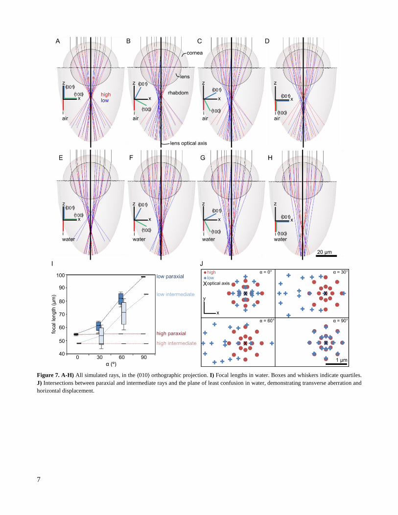
paraxial rays where β = 0°. Ray tracing reveals that focal lengths for high and low paraxial rays are within ~0.5
µm of each other if α = 0°. With increasing α, the focal length of the high rays does not change, but that of low
rays almost doubles as α approaches 90˚ (Figure 7). Thus, the high ray image is always in focus in the same plane,
inside the rhabdom. When α = 0°, the low ray image is superimposed on the high ray image, but as α increases,
the low ray image shifts lower in the rhabdom, exiting the rhabdom between α = 60˚ and α = 90˚.
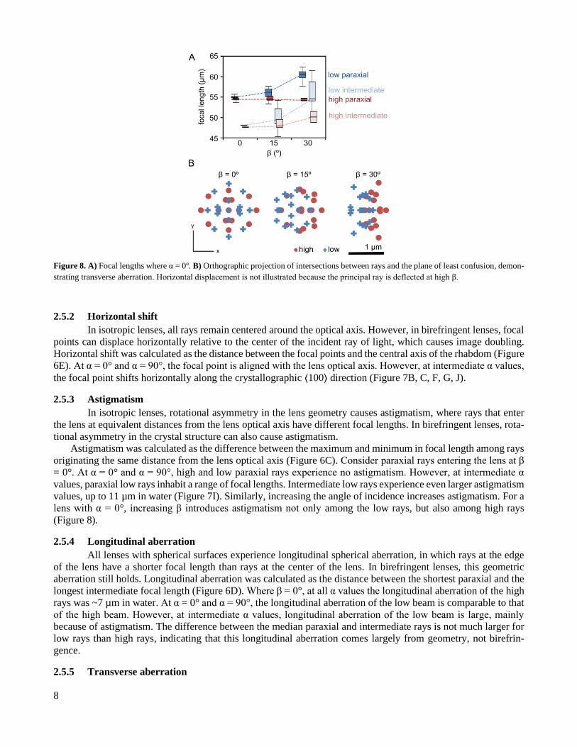
Next, consider the edges of the focal surface, determined by the focal length of the paraxial rays where β
> 0°. As β increases, the focal length of the high paraxial rays remains constant, while the focal length of the low
paraxial rays increases (Figure 8A). Consequently, a lens with α = 0° has two focal surfaces which intersect at
their centers but diverge at their peripheries.
Finally, consider the environment in which the chiton resides. Rays entering the cornea from air are re-
fracted more strongly than rays entering from water because air has a lower refractive index than water. As a result,
lenses in air have a shorter focal length than lenses in water (Figure 7A,E). However, unlike in isotropic lenses, in
birefringent lenses the focal length ratio between air and water is not fixed (Figure S6). This ratio varies between
points at equivalent radii and for varying ⟨001⟩ orientations.
7
Figure 7. A-H) All simulated rays, in the ⟨010⟩ orthographic projection. I) Focal lengths in water. Boxes and whiskers indicate quartiles.
J) Intersections between paraxial and intermediate rays and the plane of least confusion in water, demonstrating transverse aberration and
horizontal displacement.
8
Figure 8. A) Focal lengths where α = 0º. B) Orthographic projection of intersections between rays and the plane of least confusion, demon-
strating transverse aberration. Horizontal displacement is not illustrated because the principal ray is deflected at high β.
2.5.2 Horizontal shift
In isotropic lenses, all rays remain centered around the optical axis. However, in birefringent lenses, focal
points can displace horizontally relative to the center of the incident ray of light, which causes image doubling.
Horizontal shift was calculated as the distance between the focal points and the central axis of the rhabdom (Figure
6E). At α = 0° and α = 90°, the focal point is aligned with the lens optical axis. However, at intermediate α values,
the focal point shifts horizontally along the crystallographic ⟨100⟩ direction (Figure 7B, C, F, G, J).
2.5.3 Astigmatism
In isotropic lenses, rotational asymmetry in the lens geometry causes astigmatism, where rays that enter
the lens at equivalent distances from the lens optical axis have different focal lengths. In birefringent lenses, rota-
tional asymmetry in the crystal structure can also cause astigmatism.
Astigmatism was calculated as the difference between the maximum and minimum in focal length among rays
originating the same distance from the lens optical axis (Figure 6C). Consider paraxial rays entering the lens at β
= 0°. At α = 0° and α = 90°, high and low paraxial rays experience no astigmatism. However, at intermediate α
values, paraxial low rays inhabit a range of focal lengths. Intermediate low rays experience even larger astigmatism
values, up to 11 µm in water (Figure 7I). Similarly, increasing the angle of incidence increases astigmatism. For a
lens with α = 0°, increasing β introduces astigmatism not only among the low rays, but also among high rays
(Figure 8).
2.5.4 Longitudinal aberration
All lenses with spherical surfaces experience longitudinal spherical aberration, in which rays at the edge
of the lens have a shorter focal length than rays at the center of the lens. In birefringent lenses, this geometric
aberration still holds. Longitudinal aberration was calculated as the distance between the shortest paraxial and the
longest intermediate focal length (Figure 6D). Where β = 0°, at all α values the longitudinal aberration of the high
rays was ~7 µm in water. At α = 0° and α = 90°, the longitudinal aberration of the low beam is comparable to that
of the high beam. However, at intermediate α values, longitudinal aberration of the low beam is large, mainly
because of astigmatism. The difference between the median paraxial and intermediate rays is not much larger for
low rays than high rays, indicating that this longitudinal aberration comes largely from geometry, not birefrin-
gence.
2.5.5 Transverse aberration
9
Longitudinal aberration, astigmatism, and horizontal shift blur and distort images. As a result, light origi-
nating from a point source focuses to a region of least confusion instead of a point. A detector placed at the position
of the region of least confusion will therefore record the least blurry image. The size of the region of least confusion
is defined as the size of the ellipse which encompasses the intersections of all rays with the plane of the region of
least confusion (Figure 6E). The lengths of the ellipse half-axes indicate transverse aberration, and the difference
between those lengths is a supplemental metric of astigmatism. Larger, less symmetric regions of least confusion
produce low image quality.
In an isotropic lens, the region of least confusion is circular for lenses without astigmatism and elliptical
for lenses with astigmatism. In this birefringent lens, the region of least confusion can exhibit a more complex
shape. For β = 0°, high rays exhibit a circular region of least confusion when α > 0° and a slightly elliptical region
when α = 0°, while low rays exhibit an elliptical region of least confusion at α = 0° and α = 90° (Figure 7J). At
intermediate α values, low rays focus to a larger, asymmetric region of least confusion (Figure 7J). Asymmetry
becomes even more pronounced when β > 0° (Figure 8B).
3 Discussion
3.1 Lens microstructure and growth
The microstructure of the lens suggests a possible growth route and has implications for the ability of the
lens to transmit images. EBSD indicates that the lens contains a core region with small, equiaxed grains, and a
periphery containing larger, fan-shaped grains with grain boundaries that have characteristics of twinning. Arag-
onitic twinning occurs most commonly on {110} planes, with a ⟨001⟩ misorientation axis and 63.75˚ misorienta-
tion angle.[25] Twinning is commonly observed in geologic and other biogenic aragonites such as fish otoliths,
bivalve shells, and coral skeletons.[21,26–31] It is well documented in mollusks, including in crossed-lamellar struc-
tures such as the mesostracum and myostracum of the chiton valve,[20,21,27,32] helical fibers in the pteropod Cuvier-
ina,[33] prismatic aragonite structures in bivalves and gastropods,[29,30,34] and the prismatic tegmentum in which
chiton ocelli reside. In polycyclic twins of aragonite, the angle between grains separated by two or three twin
boundaries can be either 11.25˚ or 52.5˚. It is therefore possible that the 12° and 54° grain boundaries observed in
EBSD result from cyclic twinning in the lens core, as has been observed in foliated aragonite in other mollusks.[29–
31,35] Most polycyclic, polysynthetic, and deformation twins in geological and biogenic aragonite are coherent and
exhibit planar grain boundaries.[36,37] In contrast, twin boundaries in ocelli frequently exhibit micron-scale curva-
tures.
The nanotwins observed using TEM may limit incoherency strain at some curved grain boundaries. Further,
nanotwins may constitute a toughening mechanism which compensates for the loss in strength caused by large
grain sizes in the lens.[22] Nanotwins could be the cause of poor EBSD indexing in regions including the core of
the lens, the lens-valve interface, and some grain boundaries. Nanotwins or strain may also be responsible for
gradual changes in ⟨001⟩ axis orientation within grains. These gradual changes in orientation across the ocelli lens
are qualitatively similar but smaller than the gradual changes in the calcite ⟨0001⟩ axis across trilobite compound
eye lenses.[38] Because grain shapes and sizes vary between lens cross-sections, the absolute ⟨001⟩ orientation
varies between lens, and the lens contains nanotwins that are not detectable with EBSD, it is necessary to charac-
terize many cross-sections of many lenses on multiple length scales in order to fully understand the complex three-
dimensional microstructures of these lenses.
Etching reveals growth bands which run perpendicular to the fan-shaped microstructure observed in EBSD.
We expect the etch rate to increase wherever impurities, other structural defects, and/or strain increase the local
solubility. When crystals grow on a curved interface, fluctuations in the growth rate frequently result in the incor-
poration of impurities as growth bands that provide a record of the shape of the interface.[39] Impurities also fre-
quently segregate to grain boundaries and modulate etch rates parallel to the grain boundaries. In fact, some grain
boundaries seem to etch more rapidly. Together, EBSD, TEM, and etching illustrate a possible growth rate for the
lens. The lens may nucleate quickly as a finely twinned core, and then large fan-shaped grains grow off the core,
maintaining a curved growth surface. Nanotwins may alleviate incoherency strain associated with the curved grain
boundaries which result from this growth route.
10
3.2 Optical implications of microstructure While estimating the lens optical axis from optical images introduces some uncertainty, the range of ⟨001⟩ orientations observed with EBSD indicates that the organism does not align the ⟨001⟩ with the lens optical axis,
which is consistent with a previous study.[40] The orientation of the ⟨001⟩ axis has implications for the chiton’s
ability to see in both air and water. A. granulata live high in the intertidal zone and are exposed to air for long
periods of time. Speiser and coworkers predicted that the birefringence of the aragonitic lens might allow the
chiton to form an in-focus image of their environment both under water and in air.[15] At α = 90°, the low ray focal
length in air is close to the high ray focal length in water, so if sensory cells were placed on that plane, the retina
would collect a clear image in both air and water. However, because all ocelli we examined have α < 90°, the
positions of the high and low focal planes vary between air and water, so the birefringent lens is no more useful
than an isotropic lens for adapting to a tidal environment. Filling the entire cavity with sensory cells is thus useful
because of the large variability in focal lengths among α values and between air and water.
Simulations indicate that a lens with a crystallographic ⟨001⟩ axis that is not aligned with the lens optical
axis could be advantageous. At α = 0°, the high and low focal surfaces overlap at the center. However, because
the focal surfaces are ~7 µm apart at the image periphery, which is equal to the photoreceptor size, imaging both
the high and low focal surfaces simultaneously would result in image doubling at the image periphery. The organ-
ism could only separate the two sets of rays and limit aberrations if its photoreceptors were sensitive to polariza-
tion. However, if the chiton has spatial sensitivity but not polarization sensitivity, a lens with α > 0° would be
advantageous because the high and low focal planes would be spatially separated, allowing the chiton to limit
image doubling through spatial filtering. Still, the high ray image would be blurred by out-of-focus contributions
from the low rays, and vice versa. Furthermore, if the chiton does not have the sensory capabilities to spatially
filter focal surfaces, minimizing α would limit the blurring and doubling produced by birefringence.
Twinning is beneficial because of the dependence of focal length on crystallographic orientation. In lenses
with a varying ⟨001⟩ orientation, low ray images from different directions fall on varying focal planes. In a twinned
lens, the ⟨001⟩ axis remains constant, which ensures that all low rays converge on a single focal surface. However,
because the ⟨100⟩ and ⟨010⟩ axes of the grains in the lens are not aligned, and lenses have intermediate α-values,
horizontal displacement will cause image doubling across each grain boundary in ocelli. Doubling at each grain
boundary could cause each lens to transmit several distinct images, which is visible in images projected through
the lens (Figure S9). We did not simulate nanotwins, but because the nanotwins are smaller than the wavelength
of light, and horizontal displacements would be small in nanoscale grains, we do not expect nanotwins to impact
the optical properties of the lens.
Behavioral studies have indicated that chitons have the capability for spatial vision, and simulations indi-
cate that the spatial resolution of images transmitted through individual lenses is suited to the retina.[15] Pigmented
apertures are wider than 14 µm, but many rays outside of the 14 µm diameter experience total internal reflection
and do not influence the quality of images that reach the rhabdom. The ellipses of least confusion for rays generated
less than 14 µm from the principal ray are all smaller than 3 µm, so even the largest regions of least confusion
measured in this study are smaller than the photoreceptor size of 7 µm. Though asymmetric regions of least con-
fusion are reminiscent of comatic aberrations and astigmatism, and they degrade the image quality, the chiton does
not have the sensory spatial resolution to detect such aberrations.
4 Conclusion Microstructural analysis and simulations indicate that polycrystalline ocelli lenses are similar in optical
properties to single-crystalline lenses, which allow them to transmit useful images. While lenses exhibit diverse
grain morphology, and light reaches a different number of interfaces in each lens, all lenses we examined have
large grains which limit the number of interfaces that light crosses. This is beneficial for maximizing transmittance
and minimizing deflection, allowing more focused signals to reach the rhabdom. Image scattering is limited be-
cause the lens is populated with twin boundaries rather than randomly oriented grain boundaries.
Twinning may allow the lens to form quickly without sacrificing image quality.[28] Because a lens com-
posed of two twins has the same focal length and transmission as a single crystal lens, the lens can be composed
11
of many twins. If half of the rays entering the lens pass through a twin boundary, but the other half only pass
through one grain, all rays can still be resolved together, as if they all passed through a single crystal lens.
Behavioral studies have shown that chitons are capable of spatial imaging,[15] and this study shows that
lenses are capable of transmitting images, but the chiton’s sensory capabilities to process images from the ocelli
remain largely undocumented. The ocellus rhabdom compensates for the variability of the lens microstructure. It
is impossible to anticipate the focal length of the lens without knowing its microstructure. Thus, it is appropriate
that ocelli sensory cells fill the entire cavity below the lens. This allows the chiton to gather signal from anywhere
in the rhabdom, so it can adjust to the diversity of lens microstructures.
The lens grain structure limits image scattering through consistency of the ⟨001⟩ axis, so the main limita-
tions in image quality are longitudinal aberration, transverse aberration and birefringence. Trilobites and brit-
tlestars both have mechanisms to compensate for aberrations that result from the lens geometry, through variations
in refractive index and lens shape.[9–11] While the shape of chiton ocelli lenses has been heavily studied before,
little is known about the composition of the lenses. If the refractive index varies throughout the lens through
impurities, longitudinal and transverse aberration could be limited. The chiton could also use the rhabdom shape
to adjust to the crystallography of the lens. Aesthetes run at an angle to the shell surface rather than traveling
directly upwards, so the rhabdom angle could help the chiton adjust to the tilted ⟨001⟩ axis.[41–43] Whether the
chiton employs either of these techniques is still unknown. From this study, it is clear that the A. granulata ocellus
possesses a polycrystalline, twinned lens which is capable of transmitting useful images.
5 Experimental section
5.1 Preparation of sections For samples which were etched after EBSD, dried A. granulata shells collected in the Florida Keys were
purchased from a professional collector (Shellmama’s Quality Shells). For samples which were etched before
EBSD, dried A. granulata shells collected in Venezuela were obtained from the University of Alabama. Valves
were excised using tweezers and broken into smaller segments using a mortar and pestle. Sections were prepared
from a) valve segments with and without lenses, and b) whole lenses extracted from valves using a razor blade.
Samples were embedded in epoxy (Epo-Tek 301) and polymerized overnight at room temperature. Sections were
performed such that the plane of section was approximately normal to the surface of the valve (cross section) or
such that the plane normal was parallel to the optical axis (plan section). Lens sections were prepared by sequential
grinding using SiC paper (600, 800, and 1200 grit). Ground sections were then sequentially polished using poly-
crystalline aqueous diamond (3 µm and 1 µm), followed by alumina (0.05 µm) polishing suspensions. Polished
specimens were secured to aluminum scanning electron microscope (SEM) stubs using cyanoacrylate adhesive.
Orientation of cross and plan sections was confirmed by SEM. Sections were confirmed as “plan” if the
lens was surrounded by pigment, with micro-aesthetes running normal to the polished surface. Sections were con-
firmed as “cross” if there was a smoothly curved lower lens surface, pigment at the edge of the lower lens surface,
and, in some sections, a cornea present. All other sections were categorized as oblique. For plan sections, the
orientation of the optical axis was assumed to be normal to the plane. For cross sections, the direction of the optical
axis was approximated from optical micrographs and assumed to be in the plane.
Reference samples were prepared from pieces cut from a geological aragonite crystal, embedded with
either the ⟨001⟩ or ⟨100⟩ oriented approximately normal to the sample surface, ground, and polished as described
above. The final cross-sectional area of the samples was approximately 2 mm2.
5.2 Electron Backscatter Diffraction (EBSD) Ground and polished sections of 24 lenses, one shell section, and sections of geological aragonite were
examined using electron backscatter diffraction (EBSD). In seven samples, the plane of the section was approxi-
mately perpendicular to the surface of the valve; we refer to these as cross-sections. In fifteen samples the plane
was approximately parallel to the surface of the shell (plan sections), and in two cases it was oblique.
Uncoated samples were mounted on a 70º pre-tilted SEM sample holder and observed in a FEI Quanta
600F Environmental Field Emission SEM operated at a water vapor partial pressure of 0.9 Torr, an accelerating
voltage of 30 keV, and a working distance of 10 mm. Kikuchi patterns were collected from ground and polished
12
biological specimens (step size 0.3 µm-1.1 µm) and reference samples (step size 17 µm - 24 µm) using an Oxford
Nordllys II detector
5.3 Analysis of EBSD Data EBSD data was processed using the Oxford AZtecHKL package. Misorientation between neighboring
grains was determined using a 1º critical misorientation and orthorhombic symmetry operators.[44–46] Only grains
at least ten pixels in size were considered for grain size analysis.[47,48]
Computations for statistical analyses of grain orientation were performed using Wolfram Mathematica 10,
in part using code adapted from Leong and Carlile’s Spak.[49] The mean orientation of a given crystallographic
direction was determined by fitting the 5-parameter Kent (Fisher-Bingham) distribution. Only grains at least 2
pixels in size were considered in this analysis. In addition to the mean orientation, the most and least dense direc-
tions of the distribution, the standard deviations of the distribution along those directions, the concentration κ
(large value indicates tight alignment), and the ellipticity β (large values indicate rotational asymmetry) were de-
termined.
5.4 Etching For etching, ground and polished samples were submerged in water (~400 mL, pH = 5.5) and agitated on
a rocking table at 30 rpm for 15 minutes. For some samples, EBSD orientation maps were determined before
etching. Samples were dried with compressed air, mounted on aluminum SEM stubs using cyanoacrylate adhesive,
coated with 10 nm of platinum using a Denton Desk III sputter coater and grounded using colloidal silver paint.
Etched, coated samples were observed in a Hitachi S-3400N-II SEM operated at an accelerating voltage of 20
keV, a probe current of 50 µA and a working distance of 10 mm. Additional coated, etched samples were observed
in a Hitachi S4800-II cFEG SEM at an accelerating voltage of 15 keV, a probe current of 10 µA and a working
distance of 5 mm.
5.5 Focused Ion Beam (FIB) Preparation of TEM lamellae TEM lamellae were prepared from ground and polished cross-sections of epoxy-embedded ocelli. As judged
by EBSD data, several grain boundaries with different orientations of the lens were targeted for the liftout proce-
dure. Specifically, a dual-beam FIB/SEM (FEI Helios Nanolab) with a gallium liquid metal ion source (LMIS)
operating at an accelerating voltage of 2–30 kV was used to prepare FIB samples for TEM. A layer of protective
platinum (~300 nm) was deposited on a 2 μm x 12 μm area of interest by using the electron beam (5 kV, 1.4 nA)
through decomposition of a (methylcyclopentadienyl)-trimethyl platinum precursor gas (FEI Helios Nanolab).
Additionally, ~1 μm thick protective platinum layer was deposited on the same area using the ion beam (30 kV,
93 pA) through decomposition of the same precursor gas. Subsequently, two trenches were cut to allow for a
roughly 1.5 μm thick lamella of the lens. Next, the micromanipulator was welded onto the lamellae, and the sample
was cut loose from the bulk material. An in situ liftout of the sample was performed, and the lamellae was welded
onto a copper TEM half-grid. After thinning to about 100 nm in a sub-region of the lamellae (5 kV, 81 pA), the
thin section was cleaned at increased angles with respect to the ion-milled surface using low voltage and current
(2 kV, 28 pA), to remove amorphous material resulting from higher current milling. The final sections were
roughly 90 nm thick, as determined from the electron beam imaging in the SEM.
5.6 HRTEM and STEM Imaging Bright Field scanning TEM (BF-STEM) images of FIB-prepared lamellae were acquired on a Hitachi HD-
2300 STEM using a room temperature single tilt side-entry holder (Hitachi). Specifically, the STEM was operated
at an accelerating voltage 200 kV, using a probe current of 168 pA. 2048 × 2048 pixel images were acquired using
a dwell time of 2 µs and a pixel size of 1.4 × 1.4 Å, yielding a total electron dose of 1071 e- Å-2.
High resolution TEM (HRTEM) images of FIB-prepared lamellae were acquired on a JEOL GrandARM
300F, using a side-entry room temperature double tilt sample holder (Gatan). Specifically, the TEM was operated
at an accelerating voltage of 300 kV and a beam current of 10 µA. The electron dose of the acquired images on
the sample was calculated from the transmitted intensity to approximate ~4.8 × 10³ e- Å-2 (4096 × 4096 pixels;
pixel size 0.11 × 0.11 Å).

13
5.7 Simulations For ray tracing simulations, we defined the following interfaces: environment-cornea, cornea-lens, lens-
rhabdom, and rhabdom-shell. The former three were modeled as oblate, the latter as prolate hemi-spheroids cen-
tered on the origin, using the Cartesian equation (1). Note that in in A. granulata, lenses can take spheroidal or
triaxial ellipsoidal shape;[16] we chose to ignore the latter for simplicity.
The positive lab z-axis is identical to the surface normal of the shell and the optical axis (axis of symmetry) of the
lens. Note that the lens optical axis is distinct from the aragonite optic axis. The half-axes a and c were determined
from optical images of embedded cross sections (Table 1, Figure 6).
Table 1. Geometric Parameters.
Interface a [µm] c [µm] half space
environment-cornea 27.3 25.3 z>0
cornea-lens 20.0 18.0 z>0
lens-rhabdom 20.0 18.0 z<0
rhabdom-shell 33.0 73.0 z<0
An incident principal ray through the origin, and thus the center of the lens, was generated in the environ-
ment above the lens. In some simulations, the incident principal ray was rotated counter-clockwise around the
positive lab y-axis by an angle β (Figure 6). Eight more parallel rays in azimuthal increments of 45º were generated
in each of three rings surrounding the principal ray at a distance of 6.7 µm (paraxial), 13.3 µm (intermediate), and
20 µm (peripheral). All rays were modeled as collimated, unpolarized light with a wavelength 𝜆 = 500 nm.
For ray tracing, the environment was modeled as air (n = 1) or water (n = 1.33); the cornea as an isotropic
material with the average refractive index of aragonite (n = 1.632); the lens as a single crystal of aragonite (nα =
1.530, nβ = 1.680, nγ = 1.686); and the rhabdom was modeled as water.
The orientation of the aragonite lattice in the lens was such that [100]ar‖[100]lab , [010]ar‖[010]lab , and [001]ar‖[001]lab. In some experiments, the lattice was rotated clockwise around the positive [010] direction (lab
y-axis) by an angle α (Figure 6). In some simulations, an incoherent twin interface parallel to the lab z-plane and
through the origin was added, separating the lens into an upper segment with a lattice orientation identical to the
one described above, and a lower segment in which the aragonite lattice was rotated 64˚ counterclockwise about
the positive [001] direction. A non-twin grain boundary was simulated by rotating the [001] direction by 64˚ about
the [010] direction in the lower segment.
Aragonite exhibits biaxial birefringence. Thus, any ray propagating in aragonite has one of two eigen-
states, which are a combination of polarization and refractive index. The ray with ‘high’ eigenstate has the higher
of the two possible refractive indices for a given direction and is therefore also referred to as the ‘slow ray’. A ray
in a low eigenstate experiences a lower refractive index and is also referred to as the ‘fast ray’. Here, we use the
terms ‘high’ and ‘low’ to indicate the eigenstate of rays. Rays passing from an isotropic material into aragonite
are each split into a high and a low ray that propagate in different directions (Figure 6B). Because the high ray
experiences a higher refractive index, it is refracted more strongly than the low ray.
Depending on the angle of incidence at any given interface, rays may be partially or totally internally
reflected (Figure 6C). Calculating the direction of propagation, polarization, and intensity of rays is not trivial; we
used the Polaris engine to do so.[24] Intensities of transmitted beams were calculated assuming that the initial rays
are not polarized.
6 Acknowledgements The study resulting in this publication was assisted by a grant from the Undergraduate Research Grant
Program which is administered by Northwestern University's Office of the Provost. However, the conclusions,

14
opinions, and other statements in this publication are the author's and not necessarily those of the sponsoring
institution. This research was sponsored by the Chemistry of Life Processes Institute CAURS Fellowship.
This work made use of the EPIC facility (NUANCE Center-Northwestern University), which has received
support from the MRSEC program (NSF DMR-1121262) at the Materials Research Center, The Nanoscale Sci-
ence and Engineering Center (EEC-0118025/003), both programs of the National Science Foundation; the State
of Illinois; and Northwestern University. This work also made use of the OMM Facility supported by the MRSEC
program of the National Science Foundation (DMR-1121262) at the Materials Research Center of Northwestern
University.
We thank Alberto Pérez-Huerta (University of Alabama) for providing shell samples.
15
7 References [1] H. A. Lowenstam, Science (80-. ). 1981, 211, 1126.
[2] D. Faivre, D. Schüler, Chem. Rev. 2008, 108, 4875.
[3] T. Tan, D. Wong, P. Lee, Opt. Express 2004, 12, 4847.
[4] Y. N. Kulchin, A. V. Bezverbny, O. A. Bukin, S. S. Voznesensky, S. S. Golik, A. Y. Mayor, Y. A.
Shchipunov, I. G. Nagorny, Laser Phys. 2011, 21, 630.
[5] K. Klančnik, K. Vogel-Mikuš, M. Kelemen, P. Vavpetič, P. Pelicon, P. Kump, D. Jezeršek, A. Gianoncelli,
A. Gaberščik, J. Photochem. Photobiol. B Biol. 2014, 140, 276.
[6] A. Gal, V. Brumfeld, S. Weiner, L. Addadi, D. Oron, Adv. Mater. 2012, 24, OP77.
[7] T. Fuhrmann, S. Landwehr, M. El Rharbi-Kucki, M. Sumper, Appl. Phys. B Lasers Opt. 2004, 78, 257.
[8] P. Vukusic, J. R. Sambles, Nature 2003, 424, 852.
[9] M. R. Lee, C. Torney, A. W. Owen, Palaeontology 2007, 50, 1031.
[10] E. Clarkson, R. Levi-Setti, Nature 1975, 254, 663.
[11] J. Aizenberg, A. Tkachenko, S. Weiner, L. Addadi, G. Hendler, Nature 2001, 412, 819.
[12] J. Aizenberg, G. Hendler, J. Mater. Chem. 2004, 14, 2066.
[13] S. Yang, G. Chen, M. Megens, C. K. Ullal, Y.-J. Han, R. Rapaport, E. L. Thomas, J. Aizenberg, Adv.
Mater. 2005, 17, 435.
[14] A. Berman, J. Hanson, L. Leiserowitz, T. Koetzle, S. Weiner, L. Addadi, Science (80-. ). 1993, 259, 776.
[15] D. I. Speiser, D. J. Eernisse, S. Johnsen, Curr. Biol. 2011, 21, 665.
[16] L. R. Brooker, Revision of Acanthopleura Guilding, 1829 (Mollusca: Polyplacophora) based on light and
electron microscopy, Western Australia, 2003.
[17] P. R. Boyle, Physiological and Behavioural Studies on the Ecology of Some New Zealand Chitons, 1967.
[18] P. R. Boyle, Nature 1969, 222, 895.
[19] D. I. Speiser, D. G. DeMartini, T. H. Oakley, J. Nat. Hist. 2014, 48, 2899.
[20] I. Kobayashi, J. Akai, Jour. Geol. Soc. Japan 1994, 100, 177.
[21] M. Suzuki, H. Kim, H. Mukai, H. Nagasawa, T. Kogure, J. Struct. Biol. 2012, 180, 458.
[22] Y. A. Shin, S. Yin, X. Li, S. Lee, S. Moon, J. Jeong, M. Kwon, S. J. Yoo, Y. M. Kim, T. Zhang, H. Gao,
S. H. Oh, Nat. Commun. 2016, 7, 10772.
[23] H. Mutvei, Zool. Scr. 1978, 7, 287.
[24] W. S. T. Lam, S. McClain, G. Smith, R. A. Chipman, Optical Society of America, Jackson Hole, Wyoming,
United States, 2010.
[25] W. L. Bragg, Proc. R. Soc. A Math. Phys. Eng. Sci. 1924, 105, 16.
[26] R. W. Gauldie, D. G. A. Nelson, Comp. Biochem. Physiol. Part A Physiol. 1988, 90, 501.
[27] N. V. Wilmot, D. J. Barber, J. D. Taylor, A. L. Graham, Philos. Trans. Biol. Sci. 1992, 337, 21.
[28] M. Marsh, R. L. Sass, Science (80-. ). 1980, 208, 1262.
[29] E. M. Harper, A. G. Checa, A. B. Rodríguez-Navarro, Acta Zool. 2009, 90, 132.
[30] D. Chateigner, C. Hedegaard, H.-R. Wenk, J. Struct. Geol. 2000, 22, 1723.
[31] A. G. Checa, A. Sánchez-Navas, A. Rodríguez-Navarro, Cryst. Growth Des. 2009, 9, 4574.
[32] C. Hedegaard, H.-R. Wenk, J. Molluscan Stud. 1998, 64, 133.
[33] M. G. Willinger, A. G. Checa, J. T. Bonarski, M. Faryna, K. Berent, Adv. Funct. Mater. 2016, 26, 553.
[34] A. Checa, E. M. Harper, M. Willinger, Invertebr. Biol. 2012, 131, 19.
[35] M. Kudo, J. Kameda, K. Saruwatari, N. Ozaki, K. Okano, H. Nagasawa, T. Kogure, J. Struct. Biol. 2010,
169, 1.
[36] T. Kogure, M. Suzuki, H. Kim, H. Mukai, A. G. Checa, T. Sasaki, H. Nagasawa, J. Cryst. Growth 2014,
397, 39.
[37] Z. Huang, H. Li, Z. Pan, Q. Wei, Y. J. Chao, X. Li, Sci. Rep. 2011, 1, 148.
[38] C. Torney, M. R. Lee, A. W. Owen, Palaeontology 2013, 57, 783.
[39] G. Dhanaraj, K. Byrappa, V. Prasad, M. Dudley, Springer Handbook of Crystal Growth, Springer,
Heidelberg, 2010.
[40] L. Li, M. J. Connors, M. Kolle, G. T. England, D. I. Speiser, X. Xiao, J. Aizenberg, C. Ortiz, Science (80-
. ). 2015, 350, 952.
[41] C. Z. Fernandez, M. J. Vendrasco, B. Runnegar, Veliger 2007, 49, 51.
[42] M. J. Vendrasco, C. Z. Fernandez, D. J. Eernisse, B. Runnegar, Am. Malacol. Bull. 2008, 25, 51.
16
[43] J. M. Baxter, A. M. Jones, J. Mar. Biol. Assoc. United Kingdom 1981, 61, 65.
[44] M. I. Aroyo, J. M. Perez-Mato, D. Orobengoa, E. Tasci, G. de la Flor, A. Kirov, Bulg. Chem. Commun.
2011, 43, 183.
[45] M. I. Aroyo, J. M. Perez-Mato, C. Capillas, E. Kroumova, S. Ivantchev, G. Madariaga, A. Kirov, H.
Wondratschek, Z. Krist. 2006, 221, 15.
[46] M. I. Aroyo, A. Kirov, C. Capillas, J. M. Perez-Mato, H. Wondratschek, Acta Cryst. 2006, A62, 115.
[47] F. J. Humphreys, Scr. Mater. 2004, 51, 771.
[48] F. J. Humphreys, J. Mater. Sci. 2001, 36, 3833.
[49] P. Leong, S. Carlile, J. Neurosci. Methods 1998, 80, 191.
[50] K. Lee, W. Wagermaier, A. Masic, K. P. Kommareddy, M. Bennet, I. Manjubala, S.-W. Lee, S. B. Park,
H. Cölfen, P. Fratzl, Nat. Commun. 2012, 3, 725.
17
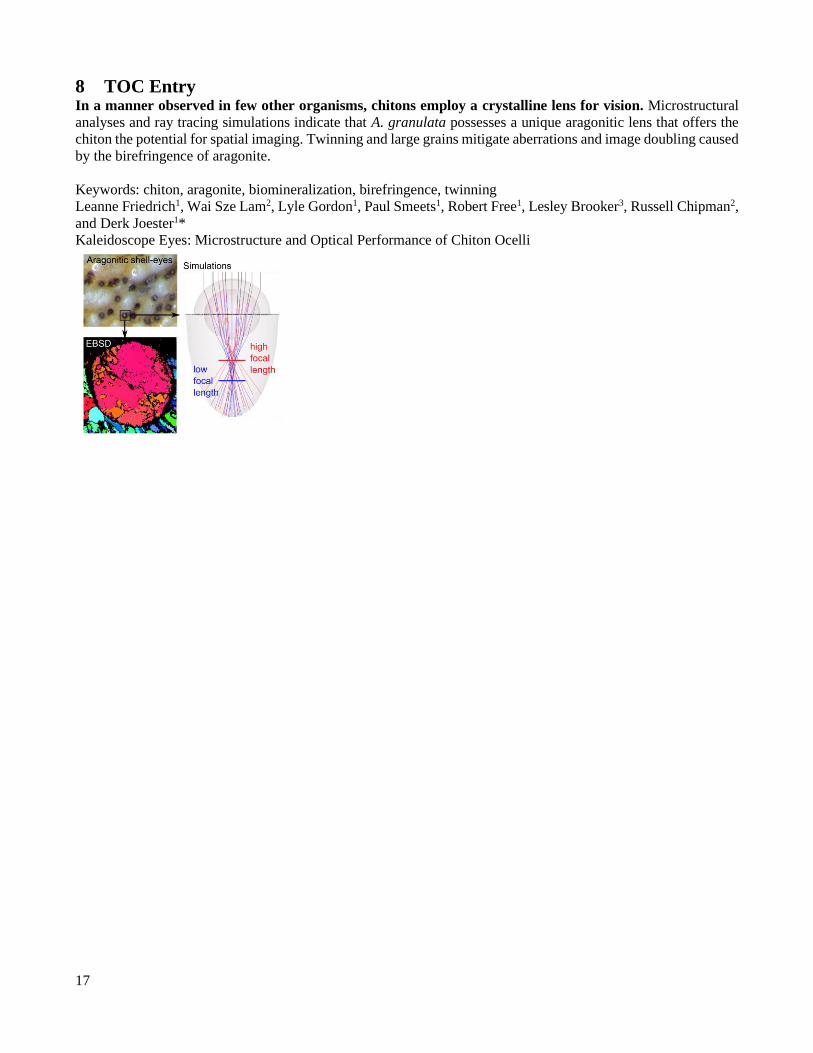
8 TOC Entry In a manner observed in few other organisms, chitons employ a crystalline lens for vision. Microstructural
analyses and ray tracing simulations indicate that A. granulata possesses a unique aragonitic lens that offers the
chiton the potential for spatial imaging. Twinning and large grains mitigate aberrations and image doubling caused
by the birefringence of aragonite.
Keywords: chiton, aragonite, biomineralization, birefringence, twinning
Leanne Friedrich1, Wai Sze Lam2, Lyle Gordon1, Paul Smeets1, Robert Free1, Lesley Brooker3, Russell Chipman2,
and Derk Joester1*
Kaleidoscope Eyes: Microstructure and Optical Performance of Chiton Ocelli
18
Supplemental Information for Kaleidoscope Eyes: Microstructure and Optical
Performance of Chiton Ocelli Leanne Friedrich1, Wai Sze Lam2, Lyle Gordon1, Paul Smeets1, Robert Free1, Lesley Brooker3, Russell Chipman2,
and Derk Joester1* 1 Materials Science and Engineering, Northwestern University, Evanston, IL 60208. 2 College of Optical Sciences, University of Arizona, Tucson, AZ 85721. 3 GeneCology Research Centre, University of the Sunshine Coast, Sippy Downs, QLD 4556, Australia.
* to whom correspondence should be addressed: [email protected]
19
S1.1 Microstructure
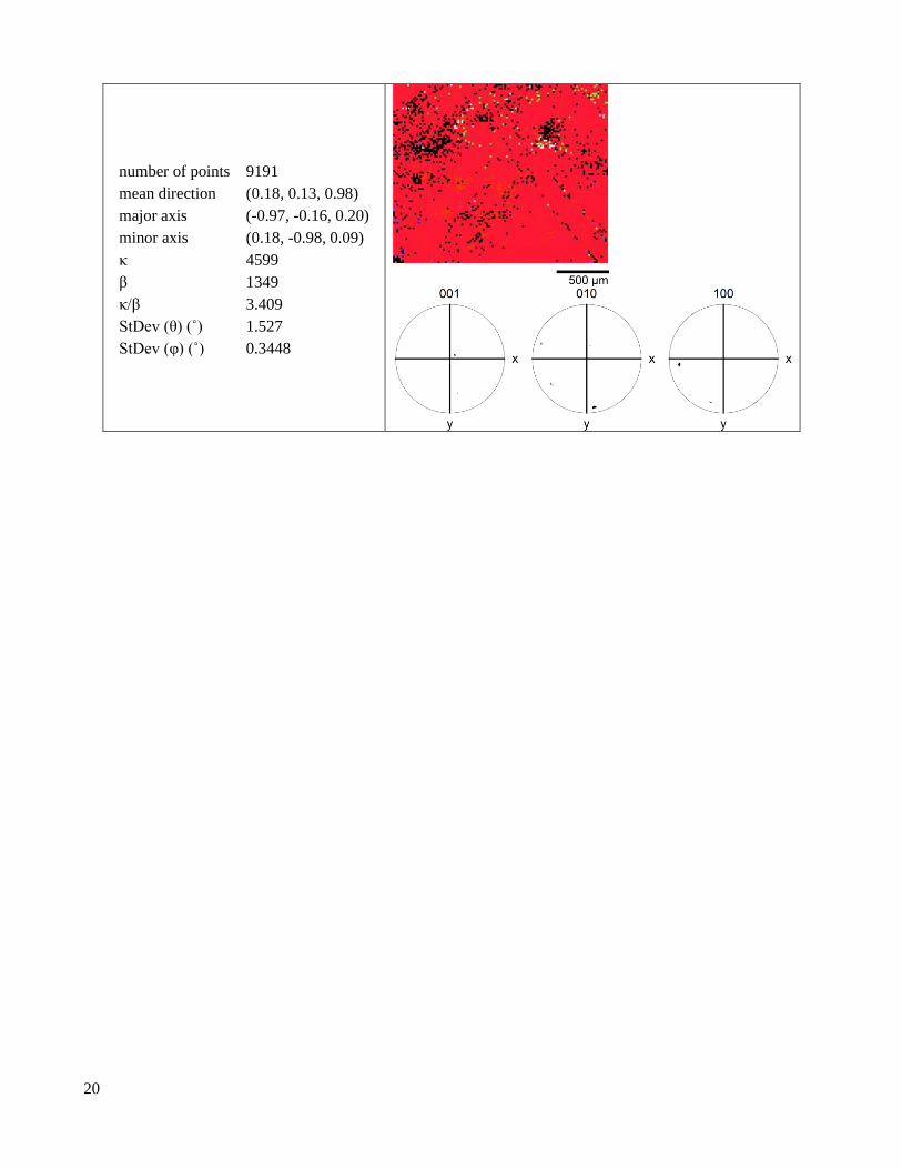
S1.1.1 Geological crystal
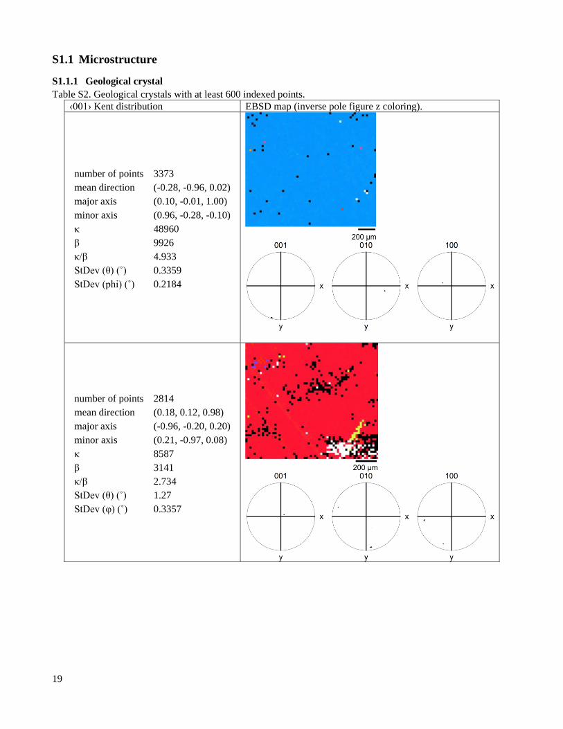
Table S2. Geological crystals with at least 600 indexed points.
‹001› Kent distribution EBSD map (inverse pole figure z coloring).
number of points 3373
mean direction (-0.28, -0.96, 0.02)
major axis (0.10, -0.01, 1.00)
minor axis (0.96, -0.28, -0.10)
κ 48960
β 9926
κ/β 4.933
StDev (θ) (˚) 0.3359
StDev (phi) (˚) 0.2184
number of points 2814
mean direction (0.18, 0.12, 0.98)
major axis (-0.96, -0.20, 0.20)
minor axis (0.21, -0.97, 0.08)
κ 8587
β 3141
κ/β 2.734
StDev (θ) (˚) 1.27
StDev (φ) (˚) 0.3357
20
number of points 9191
mean direction (0.18, 0.13, 0.98)
major axis (-0.97, -0.16, 0.20)
minor axis (0.18, -0.98, 0.09)
κ 4599
β 1349
κ/β 3.409
StDev (θ) (˚) 1.527
StDev (φ) (˚) 0.3448

21
S1.1.2 Oblique lenses
Table S3. Oblique lenses with at least 600 indexed points.
‹001› Kent distribution Optical micrograph, EBSD map (inverse pole figure z coloring).
Images are not necessarily aligned. Approximate location of EBSD
scan is shown.
number of points 2217
mean direction (-0.65, 0.41, 0.64)
major axis (-0.18, -0.90, 0.39)
minor axis (-0.74, -0.14, -0.66)
κ 1707
β 359.6
κ/β 4.747
StDev (θ) (˚) 1.841
StDev (φ) (˚) 1.16
number of points 2187
mean direction (0.35, 0.45, 0.82)
major axis (0.90, -0.43, -0.15)
minor axis (-0.28, -0.78, 0.55)
κ 635.2
β 32.59
κ/β 19.49
StDev (θ) (˚) 2.403
StDev (φ) (˚) 2.164
22
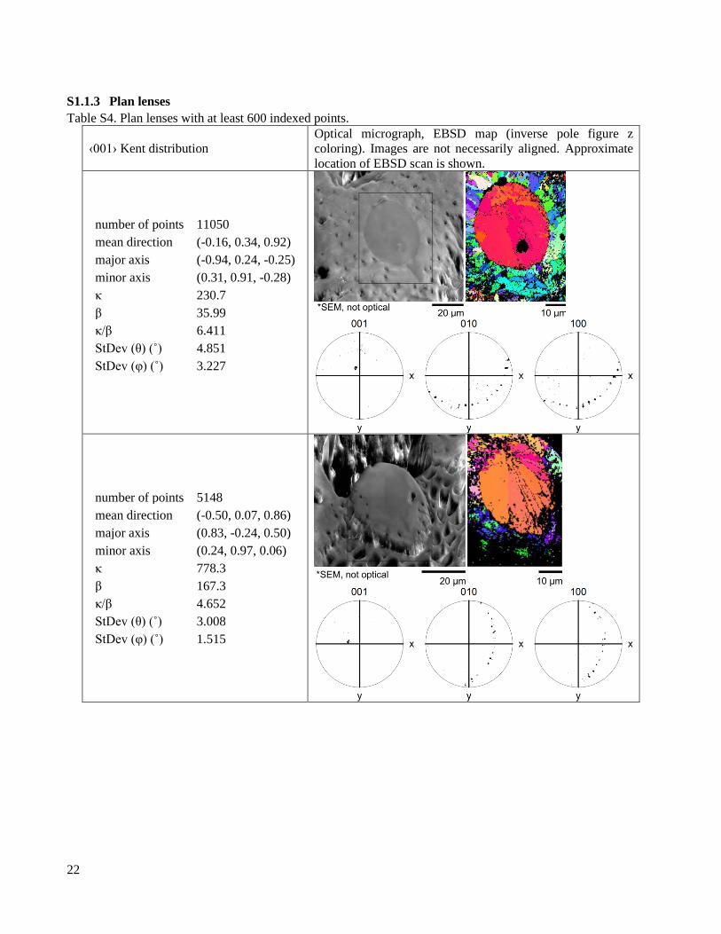
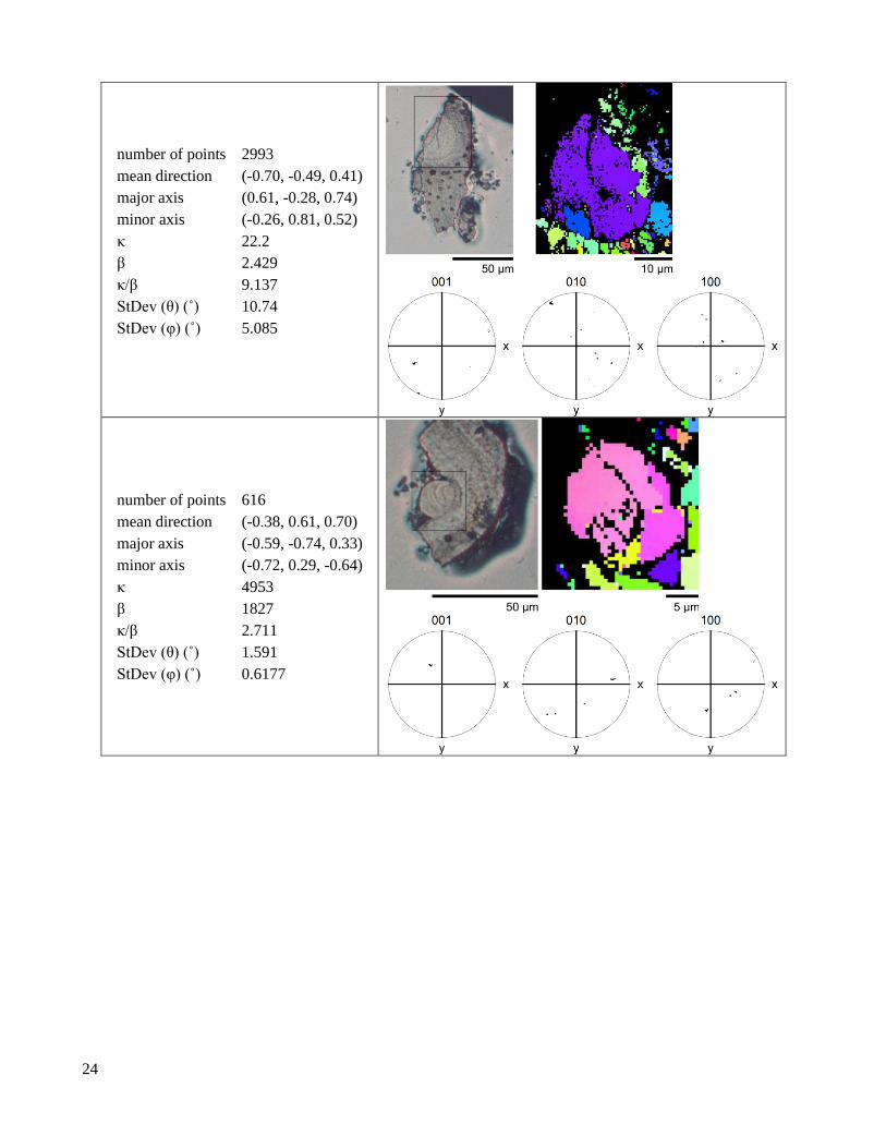
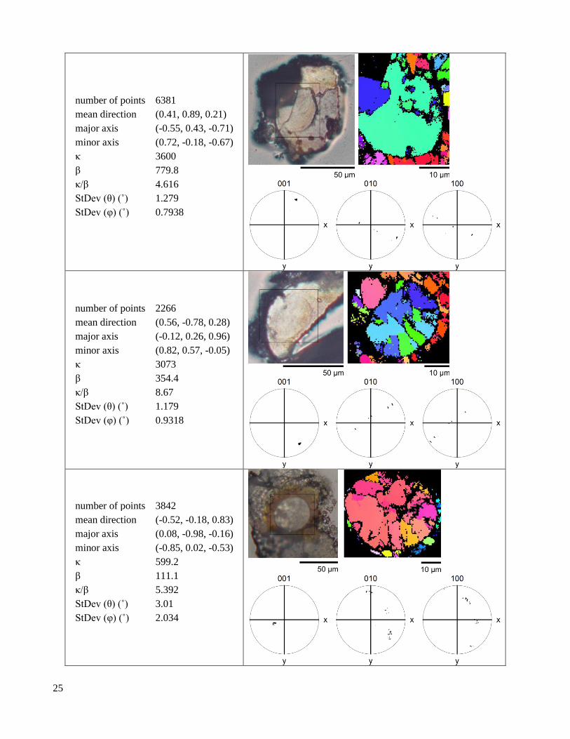
S1.1.3 Plan lenses
Table S4. Plan lenses with at least 600 indexed points.
‹001› Kent distribution
Optical micrograph, EBSD map (inverse pole figure z
coloring). Images are not necessarily aligned. Approximate
location of EBSD scan is shown.
number of points 11050
mean direction (-0.16, 0.34, 0.92)
major axis (-0.94, 0.24, -0.25)
minor axis (0.31, 0.91, -0.28)
κ 230.7
β 35.99
κ/β 6.411
StDev (θ) (˚) 4.851
StDev (φ) (˚) 3.227
number of points 5148
mean direction (-0.50, 0.07, 0.86)
major axis (0.83, -0.24, 0.50)
minor axis (0.24, 0.97, 0.06)
κ 778.3
β 167.3
κ/β 4.652
StDev (θ) (˚) 3.008
StDev (φ) (˚) 1.515

23
number of points 5896
mean direction (0.70, 0.26, 0.66)
major axis (0.40, 0.62, -0.67)
minor axis (-0.59, 0.74, 0.33)
κ 3087
β 1062
κ/β 2.907
StDev (θ) (˚) 1.847
StDev (φ) (˚) 0.793
number of points 7386
mean direction (0.26, -0.33, 0.91)
major axis (0.02, -0.94, -0.35)
minor axis (0.96, 0.11, -0.24)
κ 3024
β 984
κ/β 3.073
StDev (θ) (˚) 1.764
StDev (φ) (˚) 0.8106
24
number of points 2993
mean direction (-0.70, -0.49, 0.41)
major axis (0.61, -0.28, 0.74)
minor axis (-0.26, 0.81, 0.52)
κ 22.2
β 2.429
κ/β 9.137
StDev (θ) (˚) 10.74
StDev (φ) (˚) 5.085
number of points 616
mean direction (-0.38, 0.61, 0.70)
major axis (-0.59, -0.74, 0.33)
minor axis (-0.72, 0.29, -0.64)
κ 4953
β 1827
κ/β 2.711
StDev (θ) (˚) 1.591
StDev (φ) (˚) 0.6177
25
number of points 6381
mean direction (0.41, 0.89, 0.21)
major axis (-0.55, 0.43, -0.71)
minor axis (0.72, -0.18, -0.67)
κ 3600
β 779.8
κ/β 4.616
StDev (θ) (˚) 1.279
StDev (φ) (˚) 0.7938
number of points 2266
mean direction (0.56, -0.78, 0.28)
major axis (-0.12, 0.26, 0.96)
minor axis (0.82, 0.57, -0.05)
κ 3073
β 354.4
κ/β 8.67
StDev (θ) (˚) 1.179
StDev (φ) (˚) 0.9318
number of points 3842
mean direction (-0.52, -0.18, 0.83)
major axis (0.08, -0.98, -0.16)
minor axis (-0.85, 0.02, -0.53)
κ 599.2
β 111.1
κ/β 5.392
StDev (θ) (˚) 3.01
StDev (φ) (˚) 2.034
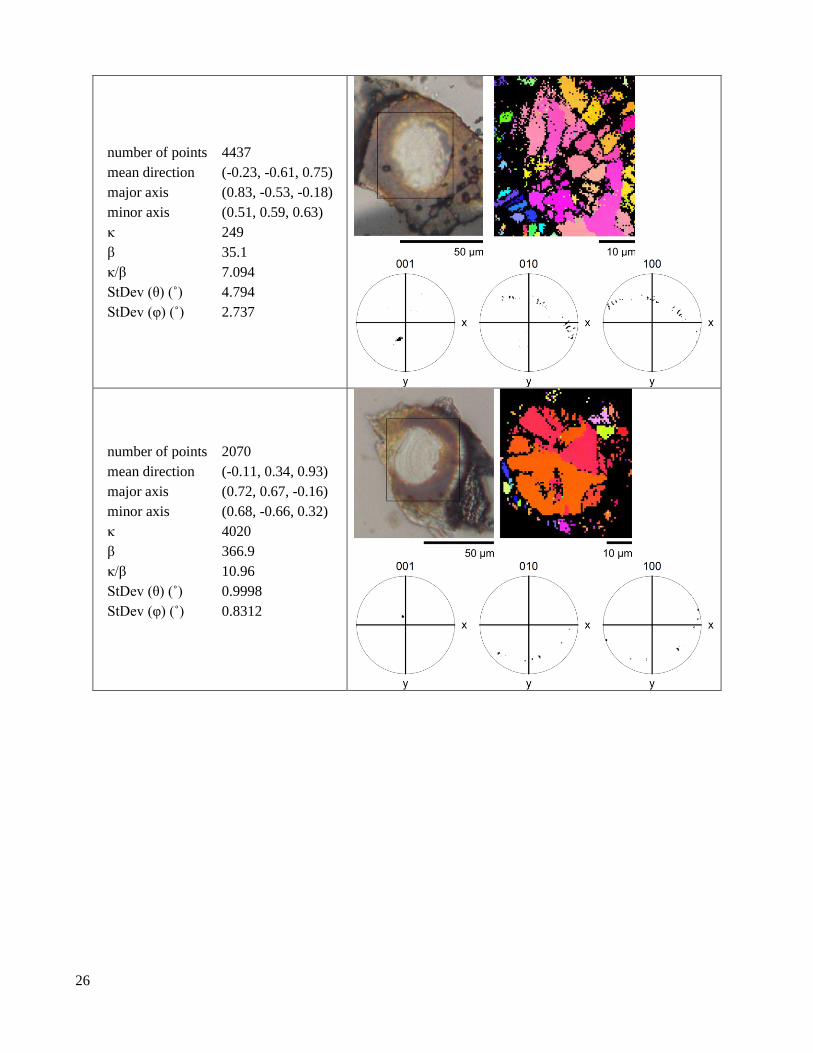
26
number of points 4437
mean direction (-0.23, -0.61, 0.75)
major axis (0.83, -0.53, -0.18)
minor axis (0.51, 0.59, 0.63)
κ 249
β 35.1
κ/β 7.094
StDev (θ) (˚) 4.794
StDev (φ) (˚) 2.737
number of points 2070
mean direction (-0.11, 0.34, 0.93)
major axis (0.72, 0.67, -0.16)
minor axis (0.68, -0.66, 0.32)
κ 4020
β 366.9
κ/β 10.96
StDev (θ) (˚) 0.9998
StDev (φ) (˚) 0.8312

27
number of points 2086
mean direction (-0.24, 0.36, 0.90)
major axis (0.51, -0.75, 0.43)
minor axis (0.83, 0.56, -0.01)
κ 3813
β 1548
κ/β 2.462
StDev (θ) (˚) 2.143
StDev (φ) (˚) 0.6887
number of points 5026
mean direction (0.07, 0.05, 0.99)
major axis (-0.68, -0.73, 0.08)
minor axis (0.73, -0.68, -0.02)
κ 654.5
β 219.5
κ/β 2.982
StDev (θ) (˚) 3.996
StDev (φ) (˚) 1.625
28
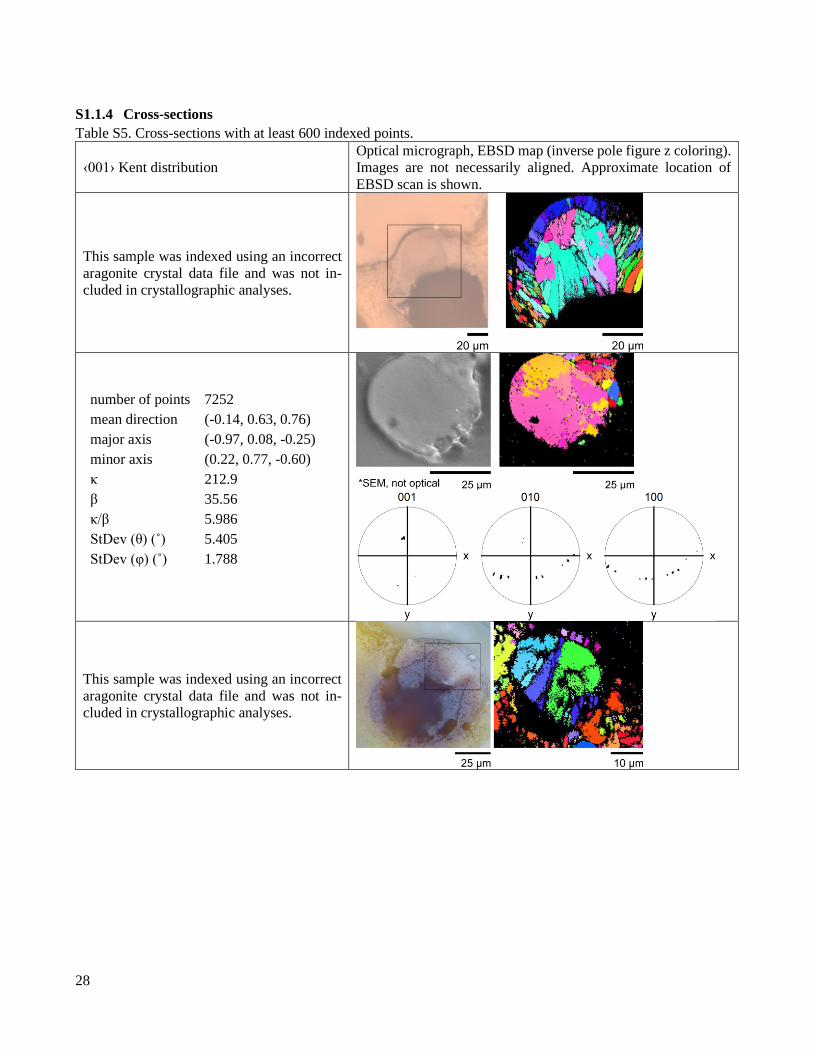
S1.1.4 Cross-sections
Table S5. Cross-sections with at least 600 indexed points.
‹001› Kent distribution
Optical micrograph, EBSD map (inverse pole figure z coloring).
Images are not necessarily aligned. Approximate location of
EBSD scan is shown.
This sample was indexed using an incorrect
aragonite crystal data file and was not in-
cluded in crystallographic analyses.
number of points 7252
mean direction (-0.14, 0.63, 0.76)
major axis (-0.97, 0.08, -0.25)
minor axis (0.22, 0.77, -0.60)
κ 212.9
β 35.56
κ/β 5.986
StDev (θ) (˚) 5.405
StDev (φ) (˚) 1.788
This sample was indexed using an incorrect
aragonite crystal data file and was not in-
cluded in crystallographic analyses.
29
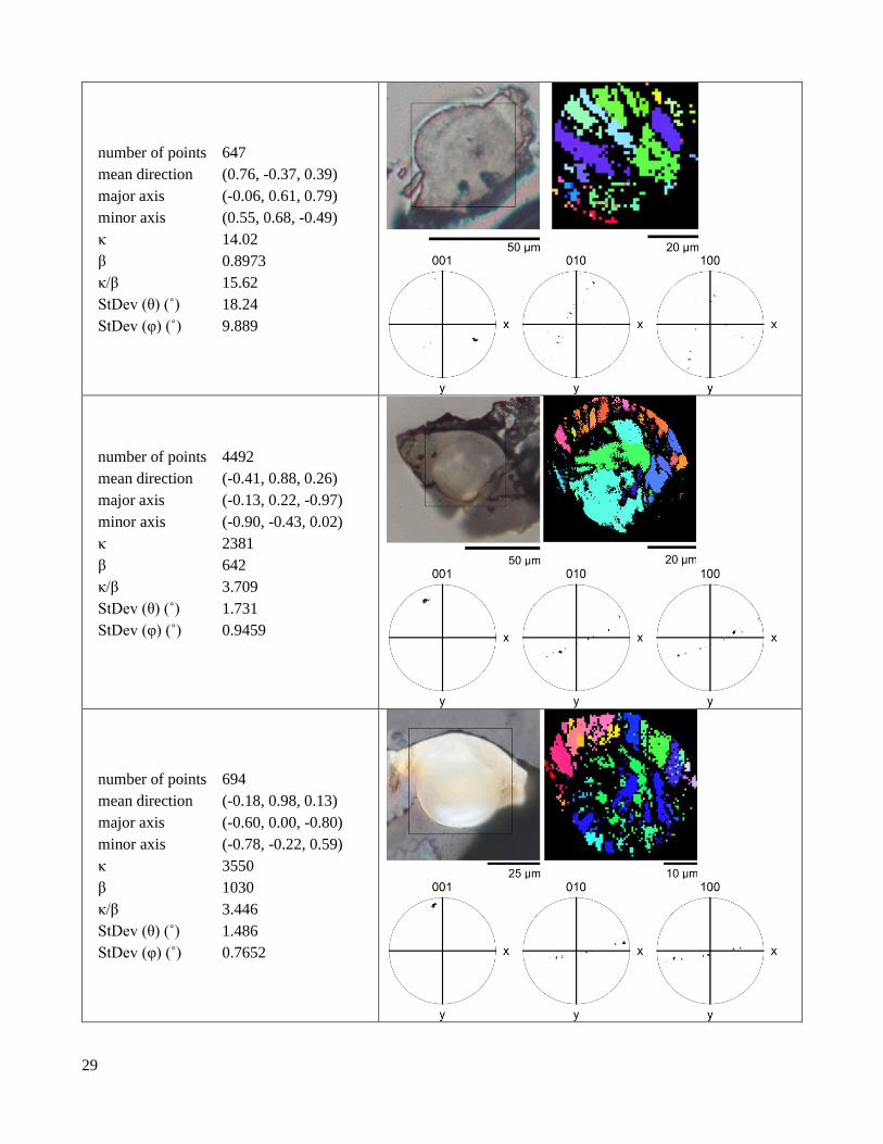
number of points 647
mean direction (0.76, -0.37, 0.39)
major axis (-0.06, 0.61, 0.79)
minor axis (0.55, 0.68, -0.49)
κ 14.02
β 0.8973
κ/β 15.62
StDev (θ) (˚) 18.24
StDev (φ) (˚) 9.889
number of points 4492
mean direction (-0.41, 0.88, 0.26)
major axis (-0.13, 0.22, -0.97)
minor axis (-0.90, -0.43, 0.02)
κ 2381
β 642
κ/β 3.709
StDev (θ) (˚) 1.731
StDev (φ) (˚) 0.9459
number of points 694
mean direction (-0.18, 0.98, 0.13)
major axis (-0.60, 0.00, -0.80)
minor axis (-0.78, -0.22, 0.59)
κ 3550
β 1030
κ/β 3.446
StDev (θ) (˚) 1.486
StDev (φ) (˚) 0.7652

30
number of points 1973
mean direction (-0.74, -0.13, 0.65)
major axis (-0.58, -0.37, -0.73)
minor axis (0.34, -0.92, 0.21)
κ 2822
β 1252
κ/β 2.254
StDev (θ) (˚) 3.216
StDev (φ) (˚) 0.7791
S1.1.5 Shell
Table S6. Shells with at least 600 indexed points.
‹001› Kent distribution EBSD map (inverse pole figure z coloring).
number of points 5980
mean direction (0.26, 0.10, 0.86)
major axis (0.60, -0.80, -0.10)
minor axis (-0.75, -0.60, 0.30)
κ 10.24
β 0.1981
κ/β 51.67
StDev (θ) (˚) 20
StDev (φ) (˚) 17.18

31
Table S7. Standard deviations of single grain ⟨001⟩ orientations within samples.
Type # pixels Long
STDEV (º)
Short
STDEV (º)
Geological 3546 0.352 0.272
Geological 3237 0.326 0.217
Geological 211 0.369 0.274
Geological 1484 0.361 0.260
Lens 665 1.066 0.435
Lens 387 0.641 0.304
Lens 728 1.767 0.283
Lens 1038 0.701 0.304
Lens 523 0.487 0.261
Lens 3641 0.912 0.406
Lens 1780 0.479 0.386
Lens 2484 1.679 0.455
Lens 4766 1.884 0.713
Lens 2281 0.603 0.424
Lens 232 0.999 0.699
Lens 5017 1.149 0.630
Lens 532 0.973 0.339
Lens 1044 0.755 0.568
Lens 3026 1.420 0.505
Lens 130 0.813 0.642
Lens 1949 1.069 0.498
Lens 503 0.684 0.231
Shell 531 0.621 0.334
Shell 383 0.379 0.256
Shell 548 0.402 0.337
Shell 319 0.350 0.259
Shell 229 0.858 0.445
Shell 159 0.305 0.227
Shell 438 0.736 0.306
Shell 195 0.372 0.260
Shell 161 0.306 0.242
Shell 124 0.550 0.380
Shell 129 0.512 0.358
Table S8. ANOVA tables of long standard deviation as a function of region (lens,
valve, geological). Because the p-value is below 0.05, these data indicate a significant
difference in single-grain overall ⟨001⟩ axis orientation distribution width between
lenses, valves, and geological crystals.
Long DF SumOfSq MeanSq FRatio PValue
Model 2 2.54172 1.27086 10.9187 0.000274
Error 30 3.4918 0.116393 Total 32 6.03351
Table S9. ANOVA table of short standard deviation as a function of region (lens,
valve, geological). Because the p-value is below 0.05, these data indicate a significant
difference in single-grain ⟨001⟩ axis orientation distribution width between lenses,
valves, and geological crystals.
Short DF SumOfSq MeanSq FRatio PValue
Model 2 0.202699 0.10135 6.8751 0.003484
Error 30 0.442247 0.014742
Total 32 0.644946
32
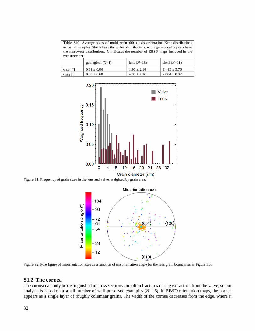
Table S10. Average sizes of multi-grain ⟨001⟩ axis orientation Kent distributions
across all samples. Shells have the widest distributions, while geological crystals have
the narrowest distributions. N indicates the number of EBSD maps included in the
measurement.
geological (N=4) lens (N=18) shell (N=11)
σshort [º] 0.31 ± 0.06 1.96 ± 2.14 14.13 ± 5.76
σlong [º] 0.89 ± 0.60 4.05 ± 4.16 27.84 ± 8.92
Figure S1. Frequency of grain sizes in the lens and valve, weighted by grain area.
Figure S2. Pole figure of misorientation axes as a function of misorientation angle for the lens grain boundaries in Figure 3B.
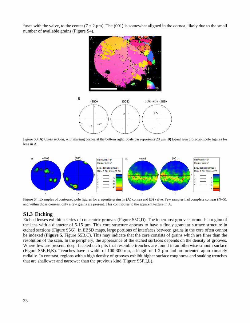
S1.2 The cornea The cornea can only be distinguished in cross sections and often fractures during extraction from the valve, so our
analysis is based on a small number of well-preserved examples (N = 5). In EBSD orientation maps, the cornea
appears as a single layer of roughly columnar grains. The width of the cornea decreases from the edge, where it
33
fuses with the valve, to the center (7 ± 2 µm). The ⟨001⟩ is somewhat aligned in the cornea, likely due to the small
number of available grains (Figure S4).
Figure S3. A) Cross section, with missing cornea at the bottom right. Scale bar represents 20 µm. B) Equal area projection pole figures for
lens in A.
Figure S4. Examples of contoured pole figures for aragonite grains in (A) cornea and (B) valve. Few samples had complete corneas (N=5),
and within those corneas, only a few grains are present. This contributes to the apparent texture in A.
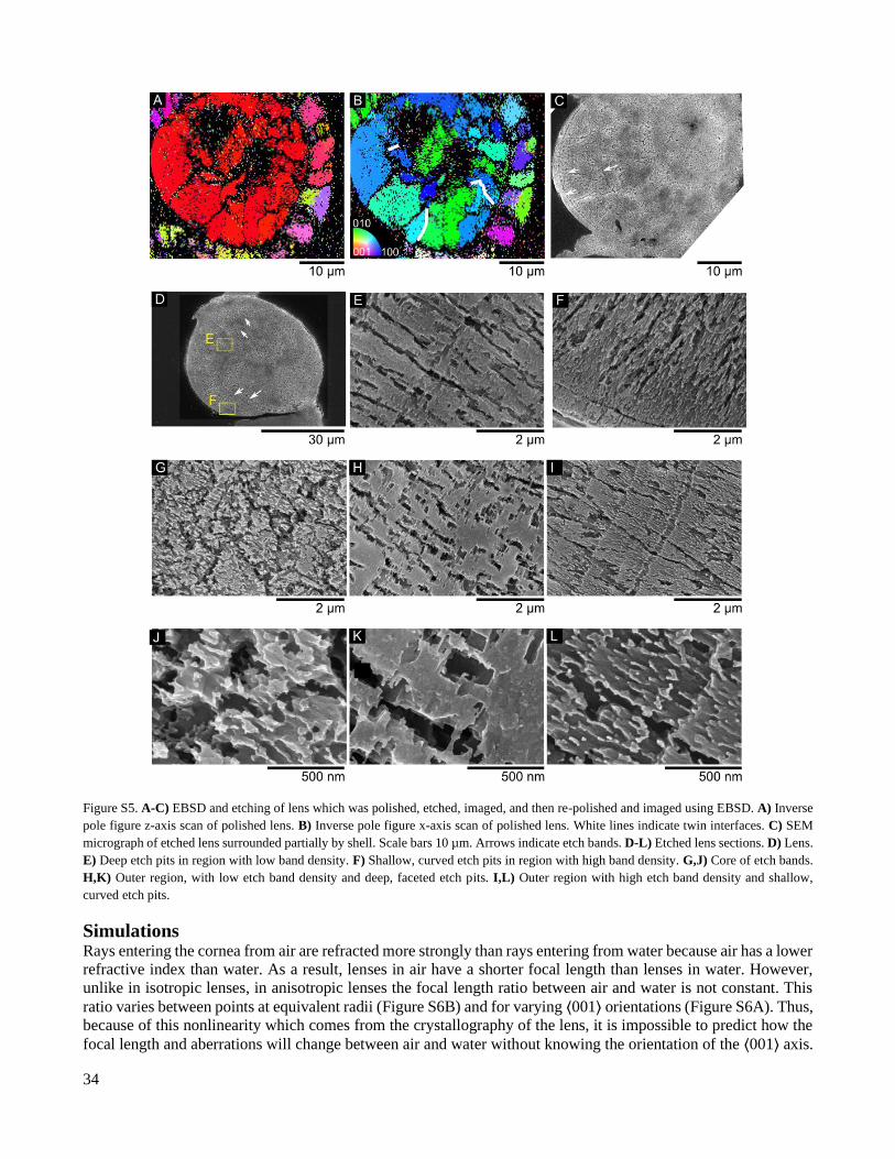
S1.3 Etching Etched lenses exhibit a series of concentric grooves (Figure S5C,D). The innermost groove surrounds a region of
the lens with a diameter of 5-15 µm. This core structure appears to have a finely granular surface structure in
etched sections (Figure S5G). In EBSD maps, large portions of interfaces between grains in the core often cannot
be indexed (Figure 5, Figure S5B,C). This may indicate that the core consists of grains which are finer than the
resolution of the scan. In the periphery, the appearance of the etched surfaces depends on the density of grooves.
Where few are present, deep, faceted etch pits that resemble trenches are found in an otherwise smooth surface
(Figure S5E,H,K). Trenches have a width of 100-300 nm, a length of 1-2 µm and are oriented approximately
radially. In contrast, regions with a high density of grooves exhibit higher surface roughness and snaking trenches
that are shallower and narrower than the previous kind (Figure S5F,I,L).
34
Figure S5. A-C) EBSD and etching of lens which was polished, etched, imaged, and then re-polished and imaged using EBSD. A) Inverse
pole figure z-axis scan of polished lens. B) Inverse pole figure x-axis scan of polished lens. White lines indicate twin interfaces. C) SEM
micrograph of etched lens surrounded partially by shell. Scale bars 10 µm. Arrows indicate etch bands. D-L) Etched lens sections. D) Lens.
E) Deep etch pits in region with low band density. F) Shallow, curved etch pits in region with high band density. G,J) Core of etch bands.
H,K) Outer region, with low etch band density and deep, faceted etch pits. I,L) Outer region with high etch band density and shallow,
curved etch pits.
Simulations Rays entering the cornea from air are refracted more strongly than rays entering from water because air has a lower
refractive index than water. As a result, lenses in air have a shorter focal length than lenses in water. However,
unlike in isotropic lenses, in anisotropic lenses the focal length ratio between air and water is not constant. This
ratio varies between points at equivalent radii (Figure S6B) and for varying ⟨001⟩ orientations (Figure S6A). Thus,
because of this nonlinearity which comes from the crystallography of the lens, it is impossible to predict how the
focal length and aberrations will change between air and water without knowing the orientation of the ⟨001⟩ axis.

35
Because the entire cell cavity is full of sensory cells, it is well-suited to detect focused light whether the chiton is
on land or underwater.
Figure S6. A) Paraxial focal length in air divided by the paraxial focal length in water. B) Ratios of individual ray focal lengths in water to
corresponding focal lengths in air for α=0º. C) Focal lengths of α=0º lenses in air and water. D) Intersections between rays and the plane of
least confusion. Both sets are centered on the lens optical axis. E, F) High ray focal regions, viewed 70º away from the ⟨010⟩ projection so
all rays can be seen. Black line indicates plane of least confusion. Dots on the black line indicate intersections with the plane of least
confusion. All other dots are focal points. Lens in (E) air and (F) water. Scale is in mm.
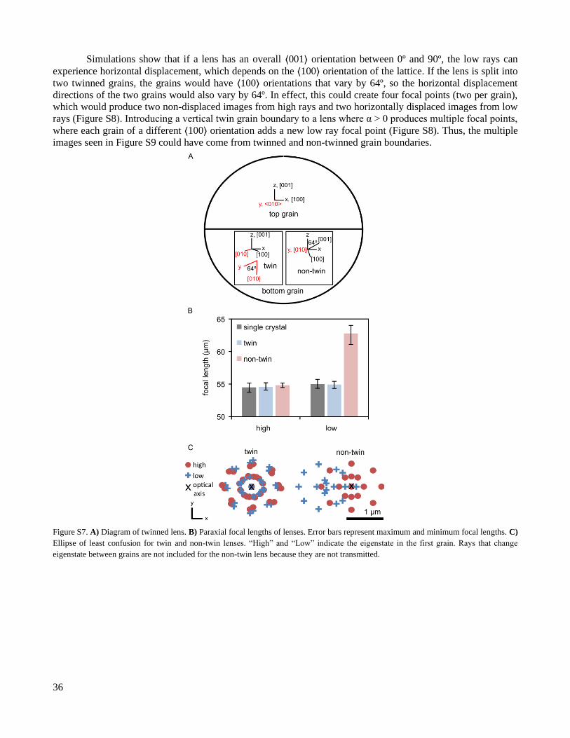
Introducing a horizontal twin grain boundary at the center of the lens changes the paraxial focal lengths
of the lens by no more than 0.16 µm, and it reduces longitudinal aberration (Figure S7B). In contrast, the non-twin
grain boundary has a larger low focal length and low ray aberrations, compared to the single-crystal lens (Figure
S7B, C). Because the non-twin interface changes the low focal length of the lens while the twin interface does not
create large changes, maintaining a high number of twin grain boundaries and low number of non-twin grain
boundaries is important.
36
Simulations show that if a lens has an overall ⟨001⟩ orientation between 0º and 90º, the low rays can
experience horizontal displacement, which depends on the ⟨100⟩ orientation of the lattice. If the lens is split into
two twinned grains, the grains would have ⟨100⟩ orientations that vary by 64º, so the horizontal displacement
directions of the two grains would also vary by 64º. In effect, this could create four focal points (two per grain),
which would produce two non-displaced images from high rays and two horizontally displaced images from low
rays (Figure S8). Introducing a vertical twin grain boundary to a lens where α > 0 produces multiple focal points,
where each grain of a different ⟨100⟩ orientation adds a new low ray focal point (Figure S8). Thus, the multiple
images seen in Figure S9 could have come from twinned and non-twinned grain boundaries.
Figure S7. A) Diagram of twinned lens. B) Paraxial focal lengths of lenses. Error bars represent maximum and minimum focal lengths. C)
Ellipse of least confusion for twin and non-twin lenses. “High” and “Low” indicate the eigenstate in the first grain. Rays that change
eigenstate between grains are not included for the non-twin lens because they are not transmitted.

37
Figure S8. A) Lens (α = 30º) containing two grains, twinned along the y-z plane. B) Intersections between rays and the ellipse of least
confusion. Right rays traveled through the right half of the lens, and left rays traveled through the left half of the lens. Three horizontally
distinct focal points (high rays, low left rays, and low right rays, marked as black X) are visible.
S1.4 Image Transmission Dozens of ocelli lenses were extracted from shells using a razor blade, placed on a glass slide in air, and
covered with a cover slip. The edges of the cover slip were sealed to the glass slide using nail polish. For compar-
ison, amorphous calcium carbonate (ACC) microlens arrays were prepared according to Lee (2012).[50] Briefly, 1
g of CaOH was dissolved in 100 mL water in a sealed jar. After three days, 23.4 µL of an aqueous solution of
Polysorbate 20 (0.22 M) was added to the solution, which was then stirred vigorously. The solution was appor-
tioned into 40 mm petri dishes. After 1 hour, microlens films formed at the surface of the solution. The films were
skimmed off the tops of the dishes onto a cover slip, and residual water was wicked from the side of the cover slip
using lint-free paper. Cover slips were dried in air and then placed film-side-down onto glass slides.
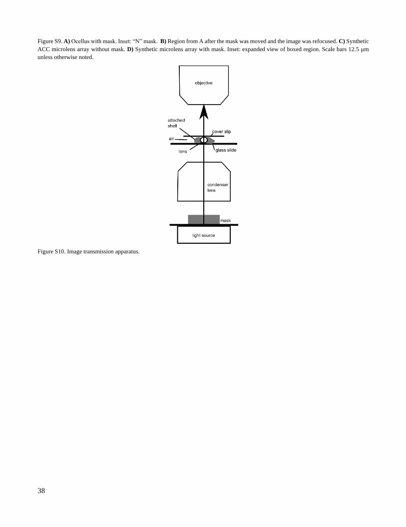
A mask was created by painting a glass slide with opaque nail polish and carving an “N” shape into the
dried paint (Figure S9A). The mask was placed directly on top of the light source of a Leica DM4000 upright
microscope (Figure S10). Using Köhler alignment, the image of the mask was focused below the ocellus lens such
that the entire microscope field of view was evenly illuminated.
To evaluate the performance of the lens, we transmitted images through isolated lenses. Optical perfor-
mance varies between lenses. In Figure S9A, the lens transmits a clear, intense “N”, but several fainter images are
projected beside the primary image. This “ghosting” effect can be seen in most lenses after moving the mask and
refocusing (Figure S9B). Ghost images in the ocelli lenses appear in varying number, size, shape, location, and
intensity. One to seven distinct images have been observed through ocelli lenses (Figure S9B). Image doubling is
not apparent in ACC lenses (Figure S9C,D).
38
Figure S9. A) Ocellus with mask. Inset: “N” mask. B) Region from A after the mask was moved and the image was refocused. C) Synthetic
ACC microlens array without mask. D) Synthetic microlens array with mask. Inset: expanded view of boxed region. Scale bars 12.5 µm
unless otherwise noted.
Figure S10. Image transmission apparatus.

39
10 Supplemental References
[1] H. A. Lowenstam, Science (80-. ). 1981, 211, 1126.
[2] D. Faivre, D. Schüler, Chem. Rev. 2008, 108, 4875.
[3] T. Tan, D. Wong, P. Lee, Opt. Express 2004, 12, 4847.
[4] Y. N. Kulchin, A. V. Bezverbny, O. A. Bukin, S. S. Voznesensky, S. S. Golik, A. Y. Mayor, Y. A.
Shchipunov, I. G. Nagorny, Laser Phys. 2011, 21, 630.
[5] K. Klančnik, K. Vogel-Mikuš, M. Kelemen, P. Vavpetič, P. Pelicon, P. Kump, D. Jezeršek, A. Gianoncelli,
A. Gaberščik, J. Photochem. Photobiol. B Biol. 2014, 140, 276.
[6] A. Gal, V. Brumfeld, S. Weiner, L. Addadi, D. Oron, Adv. Mater. 2012, 24, OP77.
[7] T. Fuhrmann, S. Landwehr, M. El Rharbi-Kucki, M. Sumper, Appl. Phys. B Lasers Opt. 2004, 78, 257.
[8] P. Vukusic, J. R. Sambles, Nature 2003, 424, 852.
[9] M. R. Lee, C. Torney, A. W. Owen, Palaeontology 2007, 50, 1031.
[10] E. Clarkson, R. Levi-Setti, Nature 1975, 254, 663.
[11] J. Aizenberg, A. Tkachenko, S. Weiner, L. Addadi, G. Hendler, Nature 2001, 412, 819.
[12] J. Aizenberg, G. Hendler, J. Mater. Chem. 2004, 14, 2066.
[13] S. Yang, G. Chen, M. Megens, C. K. Ullal, Y.-J. Han, R. Rapaport, E. L. Thomas, J. Aizenberg, Adv.
Mater. 2005, 17, 435.
[14] A. Berman, J. Hanson, L. Leiserowitz, T. Koetzle, S. Weiner, L. Addadi, Science (80-. ). 1993, 259, 776.
[15] D. I. Speiser, D. J. Eernisse, S. Johnsen, Curr. Biol. 2011, 21, 665.
[16] L. R. Brooker, Revision of Acanthopleura Guilding, 1829 (Mollusca: Polyplacophora) based on light and
electron microscopy, Western Australia, 2003.
[17] P. R. Boyle, Physiological and Behavioural Studies on the Ecology of Some New Zealand Chitons, 1967.
[18] P. R. Boyle, Nature 1969, 222, 895.
[19] D. I. Speiser, D. G. DeMartini, T. H. Oakley, J. Nat. Hist. 2014, 48, 2899.
[20] I. Kobayashi, J. Akai, Jour. Geol. Soc. Japan 1994, 100, 177.
[21] M. Suzuki, H. Kim, H. Mukai, H. Nagasawa, T. Kogure, J. Struct. Biol. 2012, 180, 458.
[22] Y. A. Shin, S. Yin, X. Li, S. Lee, S. Moon, J. Jeong, M. Kwon, S. J. Yoo, Y. M. Kim, T. Zhang, H. Gao,
S. H. Oh, Nat. Commun. 2016, 7, 10772.
[23] H. Mutvei, Zool. Scr. 1978, 7, 287.
[24] W. S. T. Lam, S. McClain, G. Smith, R. A. Chipman, Optical Society of America, Jackson Hole, Wyoming,
United States, 2010.
[25] W. L. Bragg, Proc. R. Soc. A Math. Phys. Eng. Sci. 1924, 105, 16.
[26] R. W. Gauldie, D. G. A. Nelson, Comp. Biochem. Physiol. Part A Physiol. 1988, 90, 501.
[27] N. V. Wilmot, D. J. Barber, J. D. Taylor, A. L. Graham, Philos. Trans. Biol. Sci. 1992, 337, 21.
[28] M. Marsh, R. L. Sass, Science (80-. ). 1980, 208, 1262.
[29] E. M. Harper, A. G. Checa, A. B. Rodríguez-Navarro, Acta Zool. 2009, 90, 132.
[30] D. Chateigner, C. Hedegaard, H.-R. Wenk, J. Struct. Geol. 2000, 22, 1723.
[31] A. G. Checa, A. Sánchez-Navas, A. Rodríguez-Navarro, Cryst. Growth Des. 2009, 9, 4574.
[32] C. Hedegaard, H.-R. Wenk, J. Molluscan Stud. 1998, 64, 133.
[33] M. G. Willinger, A. G. Checa, J. T. Bonarski, M. Faryna, K. Berent, Adv. Funct. Mater. 2016, 26, 553.
[34] A. Checa, E. M. Harper, M. Willinger, Invertebr. Biol. 2012, 131, 19.
[35] M. Kudo, J. Kameda, K. Saruwatari, N. Ozaki, K. Okano, H. Nagasawa, T. Kogure, J. Struct. Biol. 2010,
169, 1.
[36] T. Kogure, M. Suzuki, H. Kim, H. Mukai, A. G. Checa, T. Sasaki, H. Nagasawa, J. Cryst. Growth 2014,
397, 39.
[37] Z. Huang, H. Li, Z. Pan, Q. Wei, Y. J. Chao, X. Li, Sci. Rep. 2011, 1, 148.
[38] C. Torney, M. R. Lee, A. W. Owen, Palaeontology 2013, 57, 783.
[39] G. Dhanaraj, K. Byrappa, V. Prasad, M. Dudley, Springer Handbook of Crystal Growth, Springer,
Heidelberg, 2010.
[40] L. Li, M. J. Connors, M. Kolle, G. T. England, D. I. Speiser, X. Xiao, J. Aizenberg, C. Ortiz, Science (80-
. ). 2015, 350, 952.
[41] C. Z. Fernandez, M. J. Vendrasco, B. Runnegar, Veliger 2007, 49, 51.

40
[42] M. J. Vendrasco, C. Z. Fernandez, D. J. Eernisse, B. Runnegar, Am. Malacol. Bull. 2008, 25, 51.
[43] J. M. Baxter, A. M. Jones, J. Mar. Biol. Assoc. United Kingdom 1981, 61, 65.
[44] M. I. Aroyo, J. M. Perez-Mato, D. Orobengoa, E. Tasci, G. de la Flor, A. Kirov, Bulg. Chem. Commun.
2011, 43, 183.
[45] M. I. Aroyo, J. M. Perez-Mato, C. Capillas, E. Kroumova, S. Ivantchev, G. Madariaga, A. Kirov, H.
Wondratschek, Z. Krist. 2006, 221, 15.
[46] M. I. Aroyo, A. Kirov, C. Capillas, J. M. Perez-Mato, H. Wondratschek, Acta Cryst. 2006, A62, 115.
[47] F. J. Humphreys, Scr. Mater. 2004, 51, 771.
[48] F. J. Humphreys, J. Mater. Sci. 2001, 36, 3833.
[49] P. Leong, S. Carlile, J. Neurosci. Methods 1998, 80, 191.
[50] K. Lee, W. Wagermaier, A. Masic, K. P. Kommareddy, M. Bennet, I. Manjubala, S.-W. Lee, S. B. Park,
H. Cölfen, P. Fratzl, Nat. Commun. 2012, 3, 725.