What is the color science impact

of droplet size variation?

See the Appendix for a description of the color science model

Robert Cornell

Print System Science

March 2011

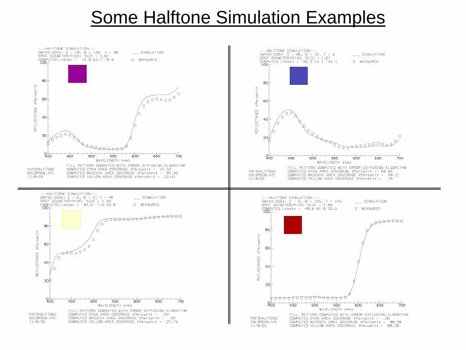
Some Halftone Simulation Examples

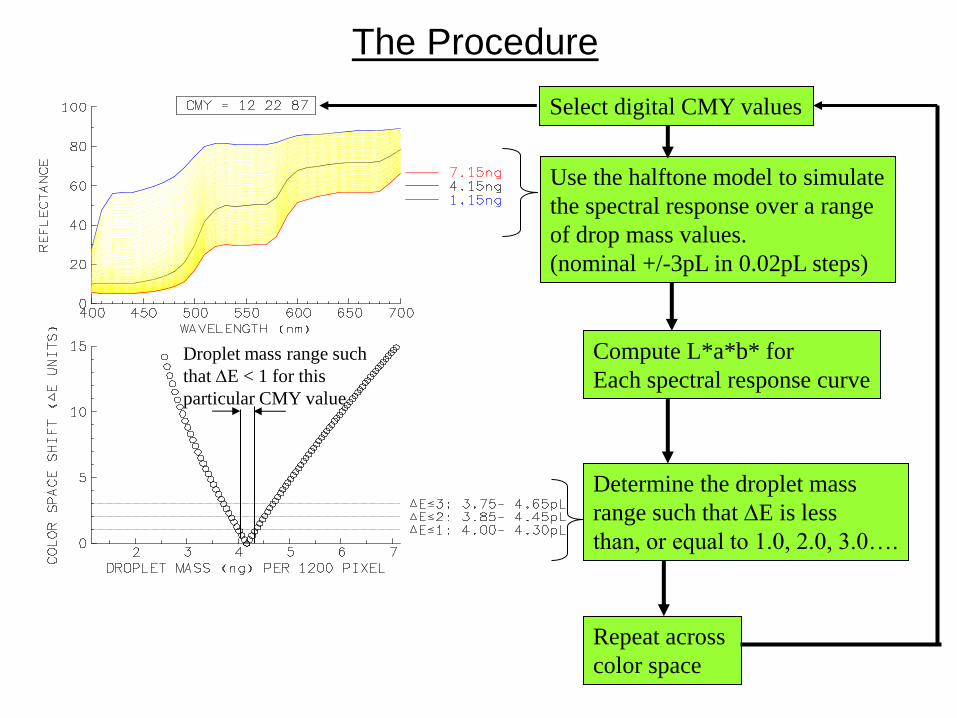
The Procedure

Use the halftone model to simulate

the spectral response over a range

of drop mass values.

(nominal +/-3pL in 0.02pL steps)

Select digital CMY values

Determine the droplet mass

range such that DE is less

than, or equal to 1.0, 2.0, 3.0….

Repeat across

color space

Compute L*a*b* for

Each spectral response curve

Droplet mass range such

that DE < 1 for this

particular CMY value

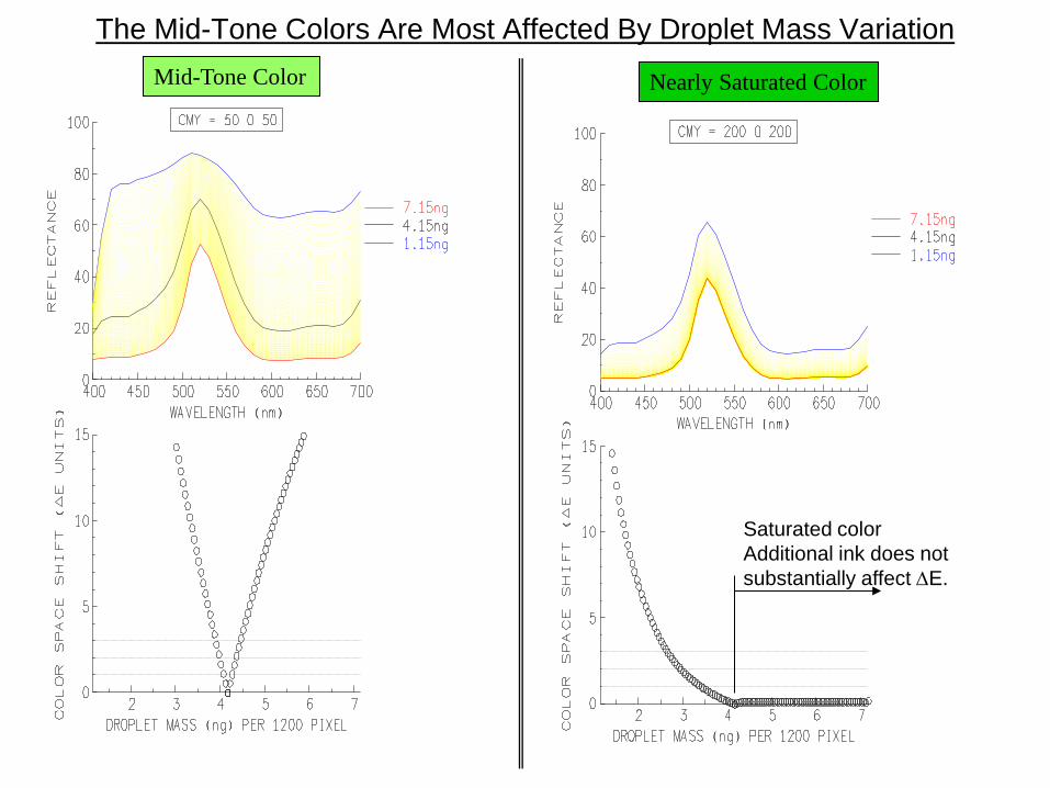
The Mid-Tone Colors Are Most Affected By Droplet Mass Variation

Mid-Tone Color Nearly Saturated Color

Saturated color

Additional ink does not

substantially affect DE.

To prevent visible color shifts in

the mid-tones, the droplet size

needs to be closely controlled DE = 3

DE = 2

DE = 1

Halftone Simulation Results

pL 1.0 -/

units E 8.6

DSlope

+/-

0.1

2p

L

+/-

0.2

7 p

L

These values are nearly identical

to the empirical direction

given by Rich Reel W

hite

Satu

rate

d

Colo

r

+/-

0.8

7 p

L

Mo

nte

Carlo

Resu

lt

6.2 DE

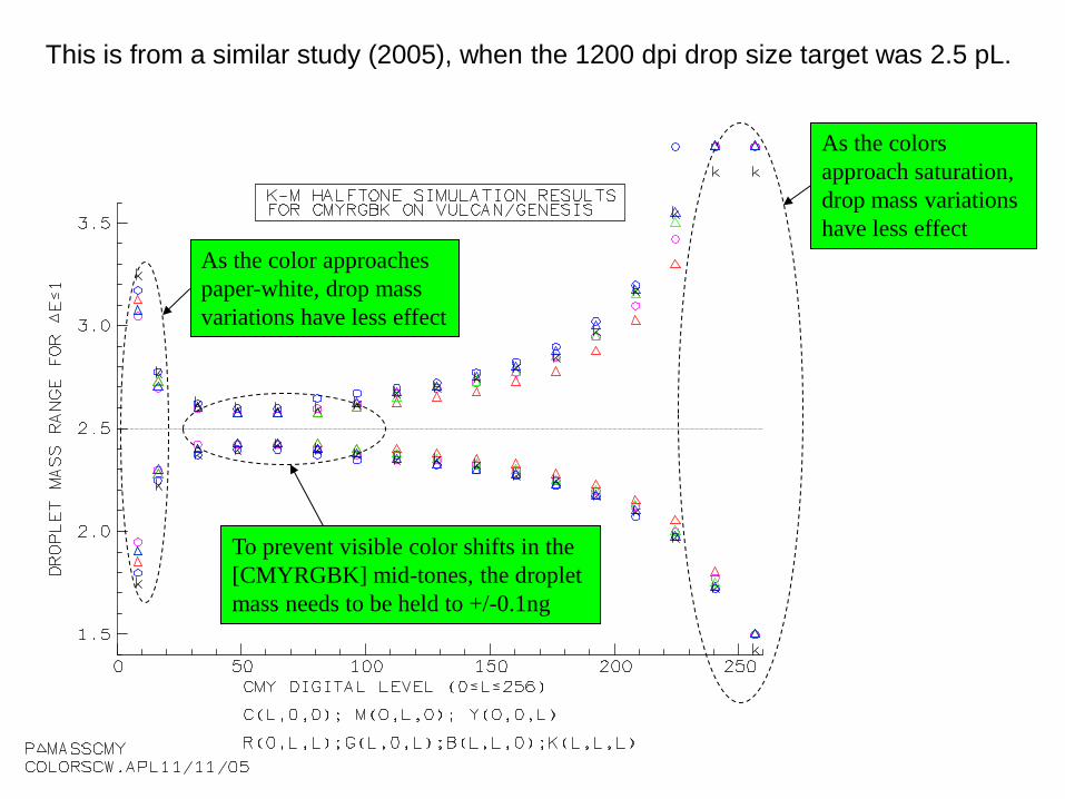
To prevent visible color shifts in the

[CMYRGBK] mid-tones, the droplet

mass needs to be held to +/-0.1ng

As the colors

approach saturation,

drop mass variations

have less effect

As the color approaches

paper-white, drop mass

variations have less effect

This is from a similar study (2005), when the 1200 dpi drop size target was 2.5 pL.

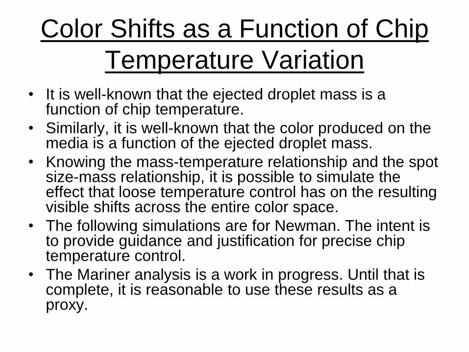
Color Shifts as a Function of Chip

Temperature Variation

• It is well-known that the ejected droplet mass is a function of chip temperature.

• Similarly, it is well-known that the color produced on the media is a function of the ejected droplet mass.

• Knowing the mass-temperature relationship and the spot size-mass relationship, it is possible to simulate the effect that loose temperature control has on the resulting visible shifts across the entire color space.

• The following simulations are for Newman. The intent is to provide guidance and justification for precise chip temperature control.

• The Mariner analysis is a work in progress. Until that is complete, it is reasonable to use these results as a proxy.

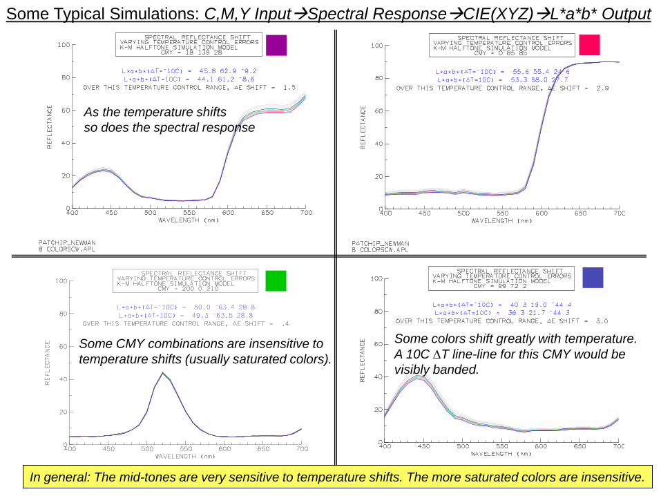
Some Typical Simulations: C,M,Y InputSpectral ResponseCIE(XYZ)L*a*b* Output

As the temperature shifts

so does the spectral response

Some colors shift greatly with temperature.

A 10C DT line-line for this CMY would be

visibly banded.

Some CMY combinations are insensitive to

temperature shifts (usually saturated colors).

In general: The mid-tones are very sensitive to temperature shifts. The more saturated colors are insensitive.

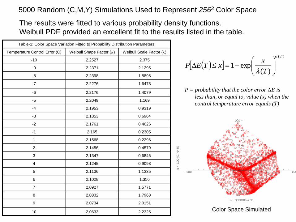
5000 Random (C,M,Y) Simulations Used to Represent 2563 Color Space

The results were fitted to various probability density functions.

Weibull PDF provided an excellent fit to the results listed in the table.

Table-1: Color Space Variation Fitted to Probability Distribution Parameters

Temperature Control Error (C) Weibull Shape Factor (a) Weibull Scale Factor (l)

-10 2.2527 2.375

-9 2.2371 2.1295

-8 2.2398 1.8895

-7 2.2276 1.6478

-6 2.2176 1.4079

-5 2.2049 1.169

-4 2.1953 0.9319

-3 2.1853 0.6964

-2 2.1761 0.4626

-1 2.165 0.2305

1 2.1568 0.2296

2 2.1456 0.4579

3 2.1347 0.6846

4 2.1245 0.9098

5 2.1136 1.1335

6 2.1028 1.356

7 2.0927 1.5771

8 2.0832 1.7968

9 2.0734 2.0151

10 2.0633 2.2325

)(

)(exp1

T

T

xxTEP

a

l

D

P = probability that the color error DE is

less than, or equal to, value (x) when the

control temperature error equals (T)

Color Space Simulated

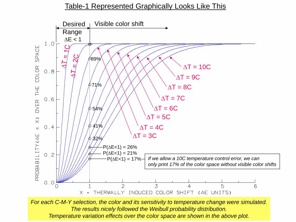
Visible color shift Desired

Range

DT = 10C

DT = 8C

DT = 5C

DT = 3C

DT = 4C

DT = 6C

DT = 7C

DT = 9C

If we allow a 10C temperature control error, we can

only print 17% of the color space without visible color shifts

P(DE<1) = 21%

P(DE<1) = 17%

P(DE<1) = 26%

32%

41%

54%

71%

89%

For each C-M-Y selection, the color and its sensitivity to temperature change were simulated.

The results nicely followed the Weibull probability distribution.

Temperature variation effects over the color space are shown in the above plot.

Table-1 Represented Graphically Looks Like This

DE < 1

Appendix

Color simulation technique

Kubelka-Munk Mixing Theory (1)

R

R

S

K

S

K

S

K

S

KR

2

1

21

2

2

Reflected Light Incident Light

Media

Colorant K = absorption coefficient

S = scattering coefficient

R = reflectance = J/I

The single constant K-M equation is often used for optically thick colorants. It has also been used

successfully in color mixing experiments on paper with foam brushes.(2)

The following discussion will illustrate

how to extend K-M mixing theory into

digital halftone printing applications.

(1) Judd & Wyszecki, Color In Business, Science and Industry, (1975). (2) Kang, H.R., Journal of Imaging Technology, Vol. 17, No.2, (1991).

For over half a century, K-M has been used to predict color in cases involving papers, dyes,

plastics, paints and textiles.

SjdxidxKSdi

jdxKSSidxdj

)(

)(J I

dx

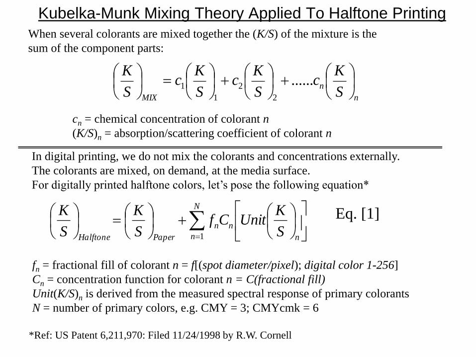
Kubelka-Munk Mixing Theory Applied To Halftone Printing

n

n

MIX S

Kc

S

Kc

S

Kc

S

K

......

2

2

1

1

When several colorants are mixed together the (K/S) of the mixture is the

sum of the component parts:

cn = chemical concentration of colorant n

(K/S)n = absorption/scattering coefficient of colorant n

In digital printing, we do not mix the colorants and concentrations externally.

The colorants are mixed, on demand, at the media surface.

For digitally printed halftone colors, let’s pose the following equation*

fn = fractional fill of colorant n = f[(spot diameter/pixel); digital color 1-256]

Cn = concentration function for colorant n = C(fractional fill)

Unit(K/S)n is derived from the measured spectral response of primary colorants

N = number of primary colors, e.g. CMY = 3; CMYcmk = 6

Eq. [1]

N

n n

nn

PaperHalftone S

KUnitCf

S

K

S

K

1

*Ref: US Patent 6,211,970: Filed 11/24/1998 by R.W. Cornell

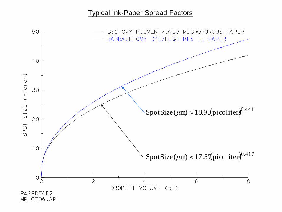
Typical Ink-Paper Spread Factors

417.0

441.0

picoliters17.57m)( SizeSpot

picoliters95.18m)( SizeSpot

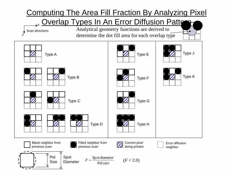
Computing The Area Fill Fraction By Analyzing Pixel

Overlap Types In An Error Diffusion Pattern

Type A

Type B

Type C

Type D

Type E

Type F

Type G

Type H

Blank neighbor from

previous scan

Filled neighbor from

previous scan

Current pixel

being printed Error diffusion

neighbor

x

y Scan directions

Pel

Size

Spot

Diameter size Pel

diameterSpot F

Type J

Type K

Analytical geometry functions are derived to

determine the dot fill area for each overlap type

(F < 2.0)

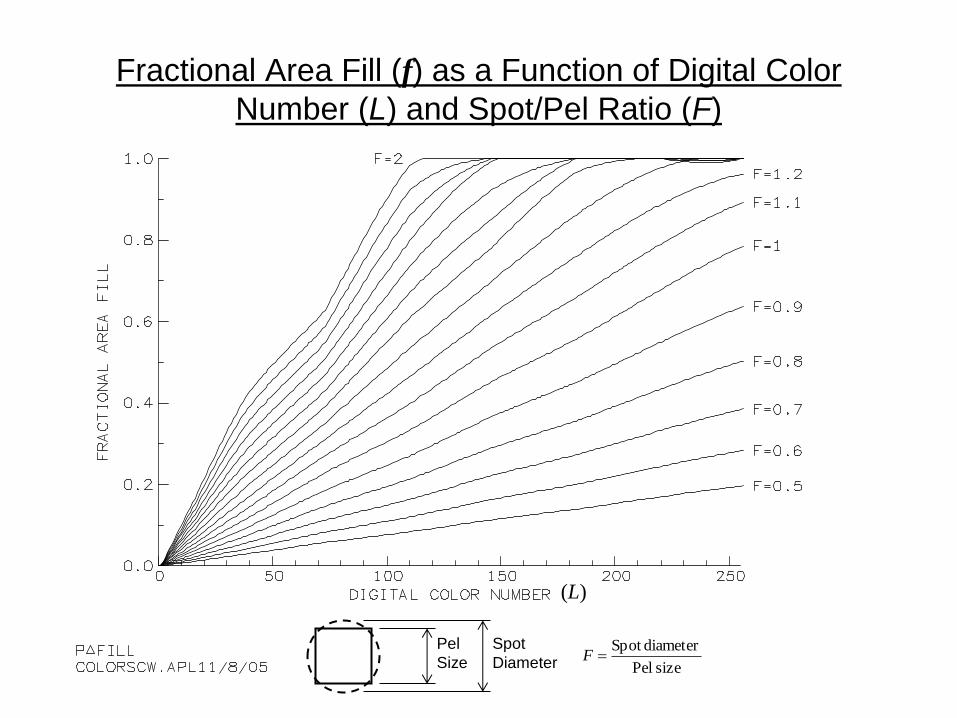
Fractional Area Fill (f) as a Function of Digital Color

Number (L) and Spot/Pel Ratio (F)

Pel

Size

Spot

Diameter size Pel

diameterSpot F

(L)

Measured Spectral Response Of Primary Colors

Cyan Magenta

Yellow

Using a spectra-photometer,

the tint ladders can be measured

for each primary color.

paper-white

saturated

paper-white

saturated

paper-white

saturated

Modeling The Ink: (K/S) Transformations

For each primary color and the blank paper, compute the following:

T

T

Paper

T

S

K

S

K

S

KUnit

S

K

S

K

S

K

R

R

S

K

h wavelengtabsorptionpeak At

FillSolid

2

Area Fill Fractional

2

1

l

l l

l

R(l) = measured spectral reflectance (400 < l < 700)nm

Eq. [2]

Eq. [3]

Eq. [4]

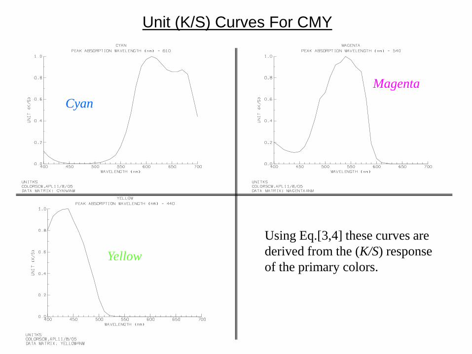
Unit (K/S) Curves For CMY

Cyan

Magenta

Yellow

Using Eq.[3,4] these curves are

derived from the (K/S) response

of the primary colors.

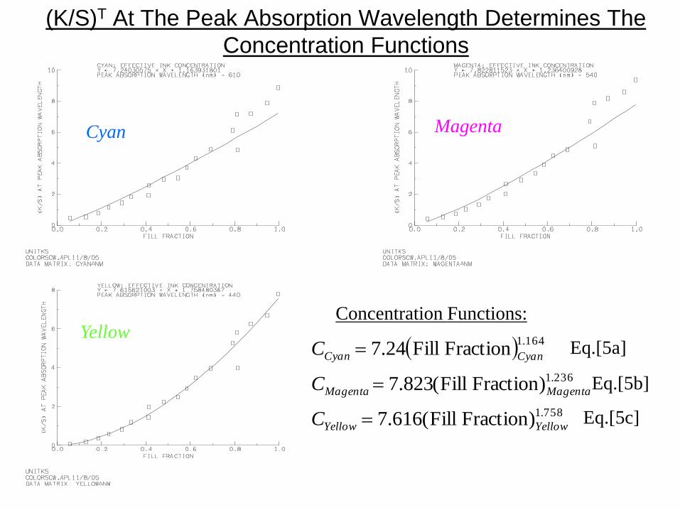
(K/S)T At The Peak Absorption Wavelength Determines The

Concentration Functions

Cyan Magenta

Yellow Concentration Functions:

758.1

236.1

164.1

) FractionFill(616.7

) FractionFill(823.7

FractionFill24.7

YellowYellow

MagentaMagenta

CyanCyan

C

C

C

Eq.[5a]

Eq.[5b]

Eq.[5c]

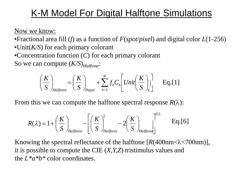
K-M Model For Digital Halftone Simulations

5.02

21)(

HalftoneHalftoneHalftone S

K

S

K

S

KR l

Now we know:

•Fractional area fill (f) as a function of F(spot/pixel) and digital color L(1-256)

•Unit(K/S) for each primary colorant

•Concentration function (C) for each primary colorant

So we can compute (K/S)Halftone:

From this we can compute the halftone spectral response R(l):

Knowing the spectral reflectance of the halftone [R(400nm<l<700nm)],

it is possible to compute the CIE (X,Y,Z) tristimulus values and

the L*a*b* color coordinates.

Eq.[1]

Eq.[6]

N

n n

nn

PaperHalftone S

KUnitCf

S

K

S

K

1

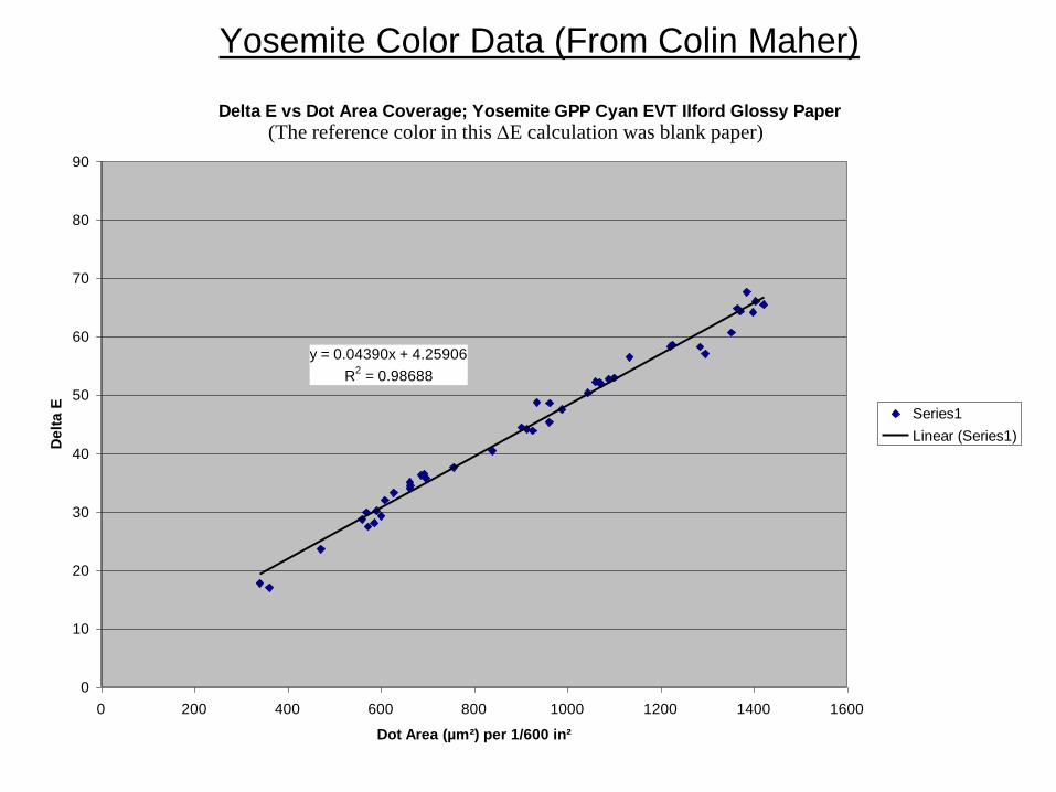
Yosemite Color Data (From Colin Maher)

Delta E vs Dot Area Coverage; Yosemite GPP Cyan EVT Ilford Glossy Paper

y = 0.04390x + 4.25906

R2 = 0.98688

0

10

20

30

40

50

60

70

80

90

0 200 400 600 800 1000 1200 1400 1600

Dot Area (µm²) per 1/600 in²

De

lta

E Series1

Linear (Series1)

(The reference color in this DE calculation was blank paper)

Does The K-M Halftone Model Still Apply?

• Characterizing the spectral response, K/S and concentration functions for an ink-media set takes several weeks, or more.

• Ink formations and media have changed many times over since this K-M halftone method was developed in 1997.

– Is it reasonable to use 1997 spectral response data of CMY-dyes and their K/S and concentration functions in an analysis of modern day CMY-pigment inks?

• Droplets and pixels are now much smaller too.

– While the K-M halftone model worked well for 18ng~80m spots, is it appropriate for today’s smaller spots?

• It will be shown on the following pages that the present K-M halftone model with the spectral response, K/S and concentration functions already presented will compare well with data taken on Yosemite-color (4-5ng) with GPP ink on Ilford glossy paper.

• Thus it is quite reasonable to use the K-M halftone model as a means of predicting the allowable droplet mass variation on a Newman ejector.

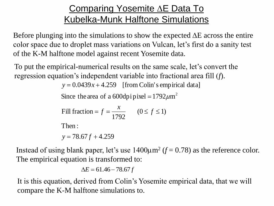
Comparing Yosemite DE Data To

Kubelka-Munk Halftone Simulations

259.467.78

:Then

)1(0 1792

fraction Fill

m1792 pixel 600dpia ofarea theSince

data] empirical sColin' [from 259.40439.0

2

fy

fx

f

xy

Before plunging into the simulations to show the expected DE across the entire

color space due to droplet mass variations on Vulcan, let’s first do a sanity test

of the K-M halftone model against recent Yosemite data.

To put the empirical-numerical results on the same scale, let’s convert the

regression equation’s independent variable into fractional area fill (f).

Instead of using blank paper, let’s use 1400m2 (f = 0.78) as the reference color.

The empirical equation is transformed to:

fE 67.7846.61 D

It is this equation, derived from Colin’s Yosemite empirical data, that we will

compare the K-M halftone simulations to.

K-M Halftone Simulation Results

Digital Level

(1-256)

Fractional Area

Fill (f)

L* a* b* DE

256 0.785

(1400m2/pel)

62.8

-26.9

-43.9 0

230 0.710

(1272m2/pel)

65.0 -27.3 -42.0 3.0

200 0.612

(1097m2/pel)

68.2 -27.2 -39.0 7.4

170 0.520

(932m2/pel)

71.6 -26.4 -35.5 12.2

140 0.433

(776m2/pel)

75.2 -24.6 -31.5 17.7

110 0.333

(597m2/pel)

79.9 -21.0 -25.9 25.6

80 0.249

(446m2/pel)

84.2 -16.4 -20.3 33.6

60 0.187

(335m2/pel)

87.6 -12.1 -15.7 40.4

Reference Color

Comparison Between Yosemite GPP-Cyan Data And The

K-M Halftone Simulations

The most important aspect of this analysis is the DE(Dmass) effect.

The f(mass) effect is known from the historical ink spread equations

shown earlier. So as long as the empirical d(DE)/df slope and the

slope resulting from the simulation is similar, we may use the existing

K-M halftone model for the Vulcan DE(Dmass) analysis.

(f)

DE

d(DE)/df = 78.7

d(DE)/df = 73.3

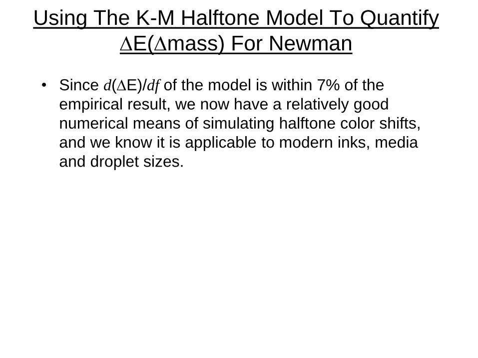
Using The K-M Halftone Model To Quantify

DE(Dmass) For Newman

• Since d(DE)/df of the model is within 7% of the

empirical result, we now have a relatively good

numerical means of simulating halftone color shifts,

and we know it is applicable to modern inks, media

and droplet sizes.