K-dimensional coding schemes in Hilbert spaces

Massimiliano Pontil

November 9, 2015

1 / 38

Plan

I Problem formulation

I Examples: PCA, K -means clustering, sparse coding,nonnegative matrix factorization, subspace clustering

I Risk bounds

I Application to the above examples

Main reference: A. Maurer and M. Pontil. K-dimensional coding schemes

in Hilbert spaces. IEEE Transactions on Information Theory, 2010

2 / 38

Problem formulation - I

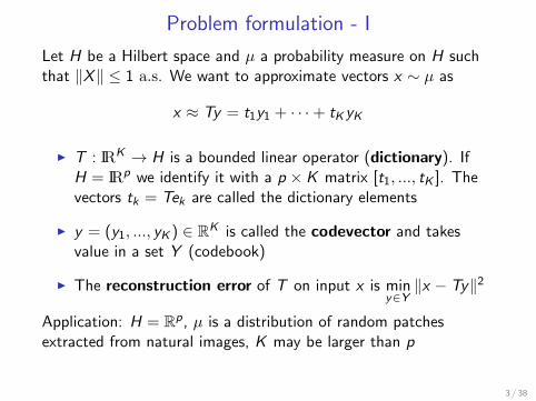
Let H be a Hilbert space and µ a probability measure on H suchthat ‖X‖ ≤ 1 a.s. We want to approximate vectors x ∼ µ as

x ≈ Ty = t1y1 + · · ·+ tKyK

I T : IRK → H is a bounded linear operator (dictionary). IfH = IRp we identify it with a p × K matrix [t1, ..., tK ]. Thevectors tk = Tek are called the dictionary elements

I y = (y1, ..., yK ) ∈ RK is called the codevector and takesvalue in a set Y (codebook)

I The reconstruction error of T on input x is miny∈Y‖x − Ty‖2

Application: H = Rp, µ is a distribution of random patchesextracted from natural images, K may be larger than p

3 / 38

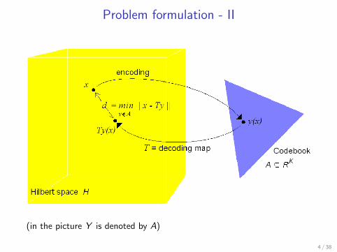
Problem formulation - II

(in the picture Y is denoted by A)

4 / 38

Problem formulation - III

LetfT (x) = min

y∈Y‖x − Ty‖2

I Average reconstruction error:

R(T ) = EfT (X ) =

∫fT (x)dµ(x)

I Think of fT as the loss and R(T ) as the expected risk of T

I Goal is to find a dictionary T within a prescribed set T , whichminimizes the risk

5 / 38

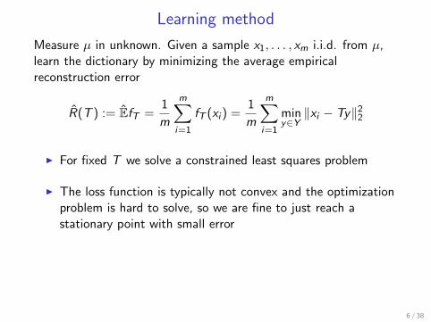
Learning method

Measure µ in unknown. Given a sample x1, . . . , xm i.i.d. from µ,learn the dictionary by minimizing the average empiricalreconstruction error

R(T ) := EfT =1

m

m∑i=1

fT (xi ) =1

m

m∑i=1

miny∈Y‖xi − Ty‖2

2

I For fixed T we solve a constrained least squares problem

I The loss function is typically not convex and the optimizationproblem is hard to solve, so we are fine to just reach astationary point with small error

6 / 38

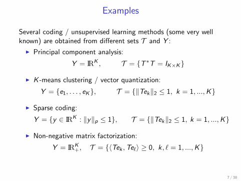
Examples

Several coding / unsupervised learning methods (some very wellknown) are obtained from different sets T and Y :

I Principal component analysis:

Y = IRK , T = T ∗T = IK×K

I K -means clustering / vector quantization:

Y = e1, . . . , eK, T = ‖Tek‖2 ≤ 1, k = 1, ...,K

I Sparse coding:

Y = y ∈ IRK : ‖y‖p ≤ 1, T = ‖Tek‖2 ≤ 1, k = 1, ...,K

I Non-negative matrix factorization:

Y = IRK+, T = 〈Tek ,Te`〉 ≥ 0, k, ` = 1, ...,K

7 / 38

PCA

If Y = RK we recover PCA, since

miny∈RK

‖x − Ty‖22 = ‖x − PT (x)‖2

2

where PT is the orthogonal projection on the range of T

I Require w.l.o.g. the tk be orthonormal (i.e. T ∗T = IK×K ), so

miny∈RK

‖xi − Ty‖22 = ‖xi‖2

2 − ‖T ∗xi‖22

I Minimizing the average reconstruction error is the same asfinding the K -dimensional linear subspace of maximumvariance

8 / 38

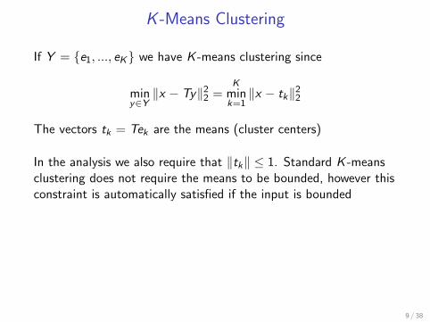
K -Means Clustering

If Y = e1, ..., eK we have K -means clustering since

miny∈Y‖x − Ty‖2

2 =K

mink=1‖x − tk‖2

2

The vectors tk = Tek are the means (cluster centers)

In the analysis we also require that ‖tk‖ ≤ 1. Standard K -meansclustering does not require the means to be bounded, however thisconstraint is automatically satisfied if the input is bounded

9 / 38

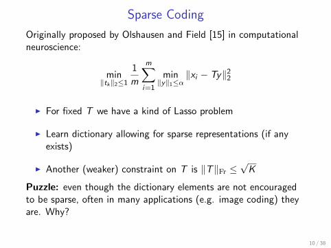
Sparse Coding

Originally proposed by Olshausen and Field [15] in computationalneuroscience:

min‖tk‖2≤1

1

m

m∑i=1

min‖y‖1≤α

‖xi − Ty‖22

I For fixed T we have a kind of Lasso problem

I Learn dictionary allowing for sparse representations (if anyexists)

I Another (weaker) constraint on T is ‖T‖Fr ≤√K

Puzzle: even though the dictionary elements are not encouragedto be sparse, often in many applications (e.g. image coding) theyare. Why?

10 / 38

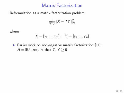
Matrix Factorization

Reformulation as a matrix factorization problem:

minT ,Y‖X − TY ‖2

Fr

whereX = [x1, ..., xm], Y = [y1, ..., ym]

I Earlier work on non-negative matrix factorization [11]:H = IRd , require that T ,Y ≥ 0

11 / 38

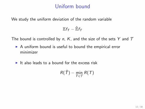
Uniform bound

We study the uniform deviation of the random variable

EfT − EfT

The bound is controlled by n, K , and the size of the sets Y and TI A uniform bound is useful to bound the empirical error

minimizer

I It also leads to a bound for the excess risk

R(T )− minT∈T

R(T )

12 / 38

Bounding the excess risk

I Recall R(T ) = EfT (X ) and R(T ) = 1m

m∑i=1

fT (xi )

I Let T ∗ such that R(T ∗) = minT∈T

R(T )

Decompose the excess risk as

R(T )−R(T ∗) = R(T ∗)−R(T ∗)︸ ︷︷ ︸unif. bound

+ R(T )−R(T ∗)︸ ︷︷ ︸≤0

+R(T )−R(T )︸ ︷︷ ︸unif. bound

Uniform bound is also nice if we can’t find T because ofnon-convexity!

13 / 38

Uniform bound

Theorem 1. If c = supT∈T ‖T‖∞ ≥ 1, Y ⊆ ‖y‖2 ≤ 1 andδ ∈ (0, 1), then with prob. ≥ 1− δ in the observed data x ∼ µm

supT∈T

EfT − EfT

≤ 6c2K

32

√π

m+ c2

√8 ln 1/δ

m

Corollary 2. If supT∈T ‖T‖∞ ≤ ∞ and Y ⊆ ‖y‖2 ≤ 1 then asm→∞

EfT −→ minT∈T

EfT

14 / 38

Uniform bound (cont.)

Theorem 3. If c = supT∈T ‖T‖∞ ≥ 1, Y ⊆ ‖y‖2 ≤ 1 andδ ∈ (0, 1), then with prob. ≥ 1− δ in the observed data x ∼ µm

supT∈T

EfT − EfT

≤ 6c2K

32

√π

m+ c2

√8 ln 1/δ

m

Method: we bound the Rademacher average,

R(F , µ) =2

mEx∼µmEσ sup

T∈T

m∑i=1

σi fT (xi )

where σ1, ..., σm are iid Rademacher. Then use

Theorem 4 ([2, 9]). If F is a [0, b]-valued function class, then withprob. ≥ 1− δ

supf∈F

Ef − Ef

≤ R(F , µ) + b

√log 1

δ

2m

15 / 38

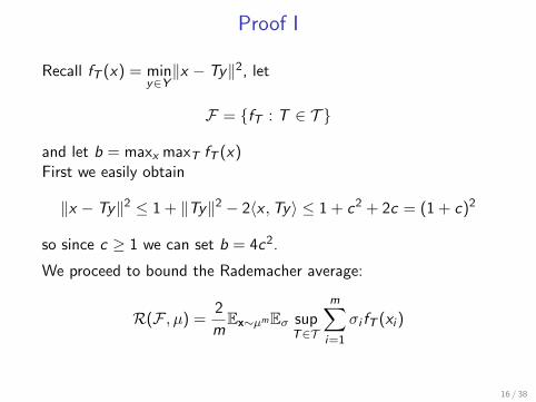
Proof I

Recall fT (x) = miny∈Y‖x − Ty‖2, let

F = fT : T ∈ T

and let b = maxx maxT fT (x)First we easily obtain

‖x − Ty‖2 ≤ 1 + ‖Ty‖2 − 2〈x ,Ty〉 ≤ 1 + c2 + 2c = (1 + c)2

so since c ≥ 1 we can set b = 4c2.

We proceed to bound the Rademacher average:

R(F , µ) =2

mEx∼µmEσ sup

T∈T

m∑i=1

σi fT (xi )

16 / 38

Proof - II

Let γ1, . . . , γm be i.i.d. N(0, 1). By the inequality [10]

Eσ supT∈T

m∑i=1

σi fT (xi ) ≤√π

2Eγ sup

T∈T

m∑i=1

γi fT (xi ) (1)

so the Rademacher average is controlled by the Gaussian average,which we bound by Slepian’s Lemma

Lemma 5 ([18]). If ΩT : T ∈ T and ΘT : T ∈ T areGaussian processes such that

E (ΩT1 − ΩT2)2 ≤ E (ΘT1 −ΘT2)2 ∀T1,T2 ∈ T

thenE sup

T∈TΩT ≤ E sup

T∈TΘT

17 / 38

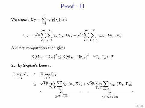
Proof - III

We choose ΩT =m∑i=1

γi fT (xi ) and

ΘT =√

8m∑i=1

K∑k=1

γik 〈xi ,Tek〉+√

2m∑i=1

K∑k,`=1

γi`k 〈Te`,Tek〉

A direct computation then gives

E (ΩT1 − ΩT2 )2 ≤ E (ΘT1 −ΘT2 )2 ∀T1,T2 ∈ T

So, by Slepian’s Lemma

E supT∈T

ΩT ≤ E supT∈T

ΘT

≤√

8E supT∈T

∑i,k

γik 〈xi ,Tek〉︸ ︷︷ ︸≤cK√

8m

+√

2E supT∈T

∑i,k,`

γik` 〈Tel ,Tek〉︸ ︷︷ ︸≤c2K

32√

2m

18 / 38

Proof IV

The last two inequalities follows by Cauchy-Schwarz’, Jensen’sinequalities and the orthogaussian properties of the γik and γik`:

E supT∈T

K∑k=1

m∑i=1

γik 〈xi ,Tek〉 ≤ cEK∑

k=1

∥∥∥∥∥m∑i=1

γikxi

∥∥∥∥∥ ≤ cK√m

and

E supT∈T

K∑k,`=1

m∑i=1

γik` 〈Tek ,Te`〉 = E supT∈T

∑k

⟨ek ,T

∗T∑i,`

γik`e`

⟩≤ Ec2

∑k

‖∑i,`

γik`e`‖

≤ c2K

√E‖∑i,`

γi`e`‖2 = c2K√Km

Multiply by√

2π/m to get a bound on the Rademacher complexity of

R (F , µ) ≤ 4cK

√π

m+ 2c2K 2

√π

m≤ 6c2K

32

√π

m.

19 / 38

Special case: K -means clustering

If Y = e1, . . . , eK and T = ‖Tek‖ ≤ 1, k = 1, ...,K we obtainK -means clustering:

fT (x) =K

mink=1‖x − Tek‖2

In this case Theorem 3 improves to

Theorem 6 (see also [4]). Let δ ∈ (0, 1). With probabilitygreater 1− δ in the sample x ∼ µm we have for all T ∈ T

Ex∼µfT (x) ≤ 1

m

m∑i=1

fT (xi ) + K

√18π

m+

√8 ln (1/δ)

m.

20 / 38

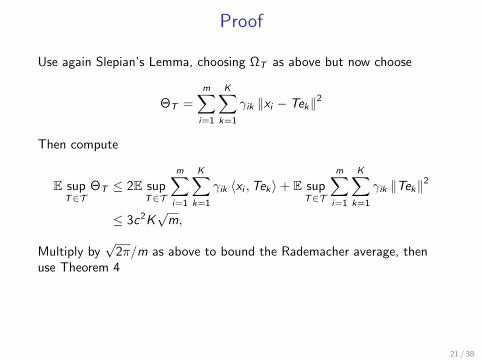
Proof

Use again Slepian’s Lemma, choosing ΩT as above but now choose

ΘT =m∑i=1

K∑k=1

γik ‖xi − Tek‖2

Then compute

E supT∈T

ΘT ≤ 2E supT∈T

m∑i=1

K∑k=1

γik 〈xi ,Tek〉+ E supT∈T

m∑i=1

K∑k=1

γik ‖Tek‖2

≤ 3c2K√m,

Multiply by√

2π/m as above to bound the Rademacher average, thenuse Theorem 4

21 / 38

Improved uniform bound

Let b = maxT∈T

max‖x‖≤1

fT (x), let ‖T‖Y = supy∈Y‖Ty‖ and assume that

ρ := supT∈T

supy∈Y‖Ty‖ ≥ 1

Theorem 7. Let δ ∈ (0, 1). With probability at least 1− δ in theobserved data x ∼ µm we have

supT∈T

EfT − EfT

≤ K√

m

(14ρ+

b

2

√ln (16mρ2)

)+ b

√ln 1/δ

2m

Idea: we decompose the function class by a finite union and use

Theorem 8. Let Fn : 1 ≤ n ≤ N be a finite collection of [0, b]-valuedfunction classes. With prob. ≥ 1− δ we have

maxn≤N

supf∈Fn

[Ef − Ef

]≤ max

n≤NRm (Fn, µ) + b

√lnN + ln

(1δ

)2m

22 / 38

Decomposition of the function class

For every map T : IRK → H there is an isometry U ∈ L(IRK ,H)and S ∈ IRK×K such that

T = US

We then have the decomposition:

F =⋃S∈SGS

GS = x 7→ miny∈Y‖x − USy‖2 : U∗U = I

where S = S ∈ IRK×K : ‖S‖Y ≤ ρ

23 / 38

Using covering numbers

Lemma 9. With probability at least 1− δ, for all T ∈ T

EfT − EfT ≤ supS∈SRm(GS , µ) +

bK

2

√ln (16mρ2)

m+

8ρ√m

+ b

√ln(1/δ)

2m.

Proof follows by a covering number argument and Theorem 8.

Step 1. There exists Sε ⊆ S, of cardinality |Sε| ≤ (4 ‖T ‖Y /ε)K 2

suchthat for every S ∈ S there exists Sε ∈ Sε with ‖S − Sε‖Y ≤ ε

Step 2. For every T ∈ T , T = US , there is Tε = USε such that‖S − Sε‖Y ≤ ε and

maxx|fT (x)− fUSε

(x)| ≤ 4 maxT

maxy‖Ty‖ε = 4ρε

Step 3. Use Theorem 8

24 / 38

Step 2

I Decompose T = US with U∗U = IK×K and S ∈ IRK×K

I Since U is an isometry ‖S‖Y = ‖T‖Y ≤ ‖T ‖YI Choose Sε ∈ Sε such that ‖Sε − S‖Y < ε

I For every x ∈ H, ‖x‖ ≤ 1, we have

|fT (x)− fUSε (x)| =

∣∣∣∣ infy∈Y‖x − USy‖2 − inf

y∈Y‖x − USεy‖2

∣∣∣∣≤ sup

y∈Y

∣∣∣‖x − USy‖2 − ‖x − USεy‖2∣∣∣

= supy∈Y|〈USεy − USy , 2x − (USy + USεy)〉|

≤ (2 + 2 ‖T ‖Y ) supy∈Y‖(Sε − S) y‖

≤ 4 ‖T ‖Y ε = 4ρε

25 / 38

Step 3

We apply Theorem 8 to the finite collection of function classesGS : S ∈ Sε to see that with probability at least 1− δ

supT∈T

Ex∼µfT (x)− 1

m

m∑i=1

fT (xi )

≤ maxS∈Sε

supU

Ex∼µfUS (x)− 1

m

m∑i=1

fUS (xi ) + 8ρε

≤ maxS∈Sε

Rm (GS , µ) + b

√ln |Sε|+ ln (1/δ)

2m+ 8ρε

≤ supS∈SRm (GS , µ) +

bK

2

√ln (16mρ2)

m+

8ρ√m

+ b

√ln (1/δ)

2m

The last line follows from the bound on |Sε|, the choice ε =√

1m

and subadditivity of the square root

26 / 38

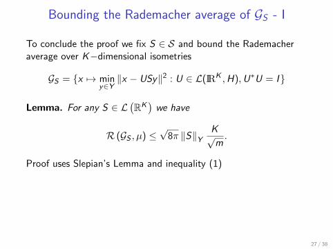
Bounding the Rademacher average of GS - I

To conclude the proof we fix S ∈ S and bound the Rademacheraverage over K−dimensional isometries

GS = x 7→ miny∈Y‖x − USy‖2 : U ∈ L(IRK ,H),U∗U = I

Lemma. For any S ∈ L(RK)

we have

R (GS , µ) ≤√

8π ‖S‖YK√m.

Proof uses Slepian’s Lemma and inequality (1)

27 / 38

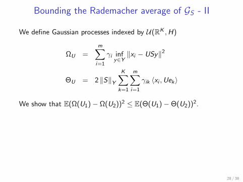
Bounding the Rademacher average of GS - II

We define Gaussian processes indexed by U(RK ,H)

ΩU =m∑i=1

γi infy∈Y‖xi − USy‖2

ΘU = 2 ‖S‖YK∑

k=1

m∑i=1

γik 〈xi ,Uek〉

We show that E(Ω(U1)− Ω(U2))2 ≤ E(Θ(U1)−Θ(U2))2.

28 / 38

Bounding the Rademacher average of GS - III

E (ΩU1 − ΩU2 )2 =m∑i=1

(infy∈Y‖xi − U1Sy‖2 − inf

y∈Y‖xi − U2S‖2

)2

≤m∑i=1

(supy∈Y‖xi − U1Sy‖2 − ‖xi − U2S‖2

)2

≤m∑i=1

supy∈Y

4〈xi , (U2 − U1)Sy〉2

≤ 4 ‖S‖2Y

m∑i=1

K∑k=1

(〈xi ,U1ek〉 − 〈xi ,U2ek〉)2

= E (ΘU1 −ΘU2 )2

Then ERγsupU

Ω(U) ≤︸︷︷︸Slepian

EsupU

ΘU ≤︸︷︷︸C.S.&Jensen

2 ‖S‖Y K√m

29 / 38

Examples

Leading term in the upper bound:

I Principal component analysis: cK√

log(m)m (can be improved

to c√

Km )

I K -means clustering: cK√

log(m)m (can be improved to c K√

m)

I Sparse coding: cK 2−1/p

√log(mK2−2/p)

m

I Non-negative matrix factorization cK 3/2√

log(mK)m

30 / 38

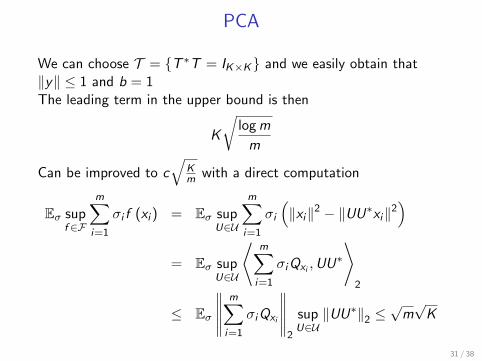
PCA

We can choose T = T ∗T = IK×K and we easily obtain that‖y‖ ≤ 1 and b = 1The leading term in the upper bound is then

K

√logm

m

Can be improved to c√

Km with a direct computation

Eσ supf ∈F

m∑i=1

σi f (xi ) = Eσ supU∈U

m∑i=1

σi

(‖xi‖2 − ‖UU∗xi‖2

)= Eσ sup

U∈U

⟨m∑i=1

σiQxi ,UU∗

⟩2

≤ Eσ

∥∥∥∥∥m∑i=1

σiQxi

∥∥∥∥∥2

supU∈U‖UU∗‖2 ≤

√m√K

31 / 38

Sparse coding

I Y = y : y ∈ RK , ‖y‖p ≤ 1

I T = T : RK → H : ‖Tek‖ ≤ 1, k = 1, ...,K

If p ≥ 1 we have

‖Ty‖ ≤K∑

k=1

|yk |‖Tek‖ ≤

(K∑

k=1

‖Tek‖q) 1

q

≤ K1q = K 1− 1

p

We then bound the estimation error by Theorem 8 with b = 1

K√m

(14K 1−1/p +

1

2

√ln(16mK 2−2/p

))+

√ln (1/δ)

2m

For p = 1 the order is comparable to K -means clustering

32 / 38

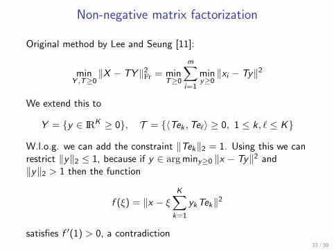
Non-negative matrix factorization

Original method by Lee and Seung [11]:

minY ,T≥0

‖X − TY ‖2Fr = min

T≥0

m∑i=1

miny≥0‖xi − Ty‖2

We extend this to

Y = y ∈ IRK ≥ 0, T = 〈Tek ,Te`〉 ≥ 0, 1 ≤ k, ` ≤ K

W.l.o.g. we can add the constraint ‖Tek‖2 = 1. Using this we canrestrict ‖y‖2 ≤ 1, because if y ∈ argminy≥0 ‖x − Ty‖2 and‖y‖2 > 1 then the function

f (ξ) = ‖x − ξK∑

k=1

ykTek‖2

satisfies f ′(1) > 0, a contradiction33 / 38

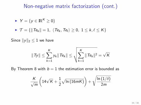
Non-negative matrix factorization (cont.)

I Y = y ∈ IRK ≥ 0

I T = ‖Tek‖ = 1, 〈Tek ,Te`〉 ≥ 0, 1 ≤ k, ` ≤ K

Since ‖y‖2 ≤ 1 we have

‖Ty‖ ≤K∑

k=1

yk‖Tek‖ ≤

√√√√ K∑k=1

‖Tek‖2 =√K

By Theorem 8 with b = 1 the estimation error is bounded as

K√m

(14√K +

1

2

√ln (16mK )

)+

√ln (1/δ)

2m

34 / 38

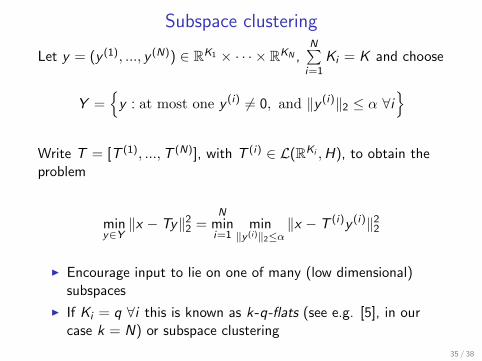
Subspace clustering

Let y = (y (1), ..., y (N)) ∈ RK1 × · · · × RKN ,N∑i=1

Ki = K and choose

Y =y : at most one y (i) 6= 0, and ‖y (i)‖2 ≤ α ∀i

Write T = [T (1), ...,T (N)], with T (i) ∈ L(RKi ,H), to obtain theproblem

miny∈Y‖x − Ty‖2

2 =N

mini=1

min‖y (i)‖2≤α

‖x − T (i)y (i)‖22

I Encourage input to lie on one of many (low dimensional)subspaces

I If Ki = q ∀i this is known as k-q-flats (see e.g. [5], in ourcase k = N) or subspace clustering

35 / 38

A bound for subspace clustering

Let y = (y (1), ..., y (N)) ∈ RK1 × · · · × RKN ,N∑i=1

Ki = K and choose

Y =y : at most one y (i) 6= 0, and ‖y (i)‖2 ≤ α ∀i

We have b = 1. W.l.o.g we can choose T (i) to be partialisometries, so

‖T‖Y ≤ maxT∈T‖Ty‖ =

Nmaxi=1

maxT (i)

max‖y (i)‖≤1

‖T (i)y (i)‖ ≤ 1

By Theorem 8 with b = 1 the estimation error is bounded as

K√m

(14 +

1

2

√ln (16m)

)+

√ln (1/δ)

2m

36 / 38

References I[1] A. Antos, L. Gyorfi, A. Gyorgy. Individual convergence rates in empirical vector quantizer design. IEEE

Transactions on Information Theory, 51(11):4013–4022, 2005.

[2] P. L. Bartlett and S. Mendelson. Rademacher and Gaussian Complexities: Risk Bounds and Structural Results.Journal of Machine Learning Research, 3: 463–482, 2002.

[3] P. Bartlett, T. Linder, G. Lugosi. The minimax distortion redundancy in empirical quantizer design. IEEETransactions on Information Theory, 44: 1802–1813, 1998.

[4] G. Biau, L. Devroye, G. Lugosi. On the performance of clustering in Hilbert spaces. IEEE Transactions onInformation Theory, 54:781–790, 2008.

[5] P.S. Bradley, O.L. Mangasarian. k-Plane clustering. Journal of Global Optimization 16(1)23-32, 2000.

[6] F. Cucker and S. Smale. On the mathematical foundations of learning, Bulletin of the American MathematicalSociety, 39 (1):1–49, 2001.

[7] W. Hoeffding. Probability inequalities for sums of bounded random variables, Journal of the AmericanStatistical Association, 58:13–30, 1963.

[8] P. O. Hoyer. Non-negative matrix factorization with sparseness constraints. Journal of Machine LearningResearch, 5:1457–1469, 2004.

[9] V. Koltchinskii and D. Panchenko. Empirical margin distributions and bounding the generalization error ofcombined classifiers, The Annals of Statistics, 30(1): 1–50, 2002.

[10] M. Ledoux, M. Talagrand. Probability in Banach Spaces, Springer, 1991.

[11] D. D. Lee and H. S. Seung. Learning the parts of objects by non-negative matrix factorization. Nature 401,788–791, 1999.

[12] S. Z. Li, X. Hou, H. Zhang, and Q. Cheng. Learning spatially localized parts-based representations. Proc.IEEE Conf. on Computer Vision and Pattern Recognition (CVPR), Vol. I, pages 207–212, Hawaii, USA, 2001.

37 / 38

References II[13] A. Maurer and M. Pontil. Generalization bounds for K -dimensional coding schemes in Hilbert spaces.

Proceedings of the 19th international conference on Algorithmic Learning Theory, pages 91, 2008,

[14] C. McDiarmid. Concentration, in Probabilistic Methods of Algorithmic Discrete Mathematics, p195-248,Springer, Berlin, 1998.

[15] B. A. Olshausen and D. J. Field. Emergence of simple-cell receptive field properties by learning a sparse codefor natural images. Nature, 381:607–609, 1996.

[16] J. Shawe-Taylor, C. K. I. Williams, N. Cristianini, J. S. Kandola. On the eigenspectrum of the Gram matrixand the generalization error of kernel-PCA. IEEE Transactions on Information Theory 51(7): 2510–2522, 2005.

[17] O. Wigelius, A. Ambroladze, J. Shawe-Taylor. Statistical analysis of clustering with applications. Preprint,2007.

[18] D. Slepian. The one-sided barrier problem for Gaussian noise. Bell System Tech. J., 41: 463–501, 1962.

[19] A.W. van der Vaart and J.A. Wallner. Weak Convergence and Empirical Processes, Springer Verlag, 1996.

[20] L. Zwald, L., O. Bousquet, and G. Blanchard. Statistical properties of kernel principal component analysis.Machine Learning 66(2-3): 259–294, 2006.

38 / 38