Juvenile Production Estimate (JPE) Calculation and Use/Application of Survival Data from Acoustically-tagged Chinook

Salmon Releases

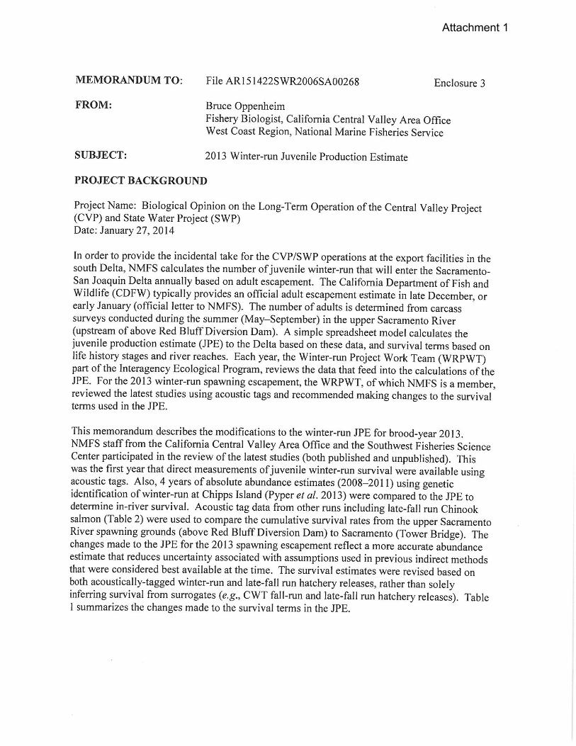
Report prepared by Bruce Oppenheim, NMFS, West Coast Region, Sacramento, California for the 2014 Annual Science Panel Review Workshop, November 6-7. Introduction Each year, NOAA’s National Marine Fisheries Service (NMFS) estimates the number of juvenile winter-run Chinook salmon expected to enter the Delta. NMFS’ June 4, 2009, biological and conference opinion on the long-term operation of the Central Valley Project and State Water Project provides an incidental take limit on natural juvenile winter-run based on the juvenile production estimate (JPE, attachment 1). Description of the Process to Calculate the Winter-run Chinook Salmon Juvenile Production Estimate (JPE) The JPE is a simple Excel spreadsheet model that starts with the official winter-run spawning escapement estimate from the California Department of Fish and Wildlife (CDFW), and subtracts a number of factors from the number of eggs produced (see enclosure 2 in Attachment 1). It contains 2 other models within it, along with the following 8 variable factors.

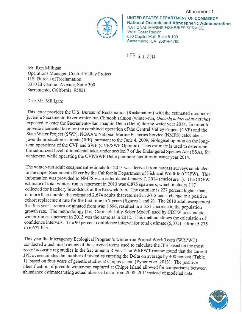
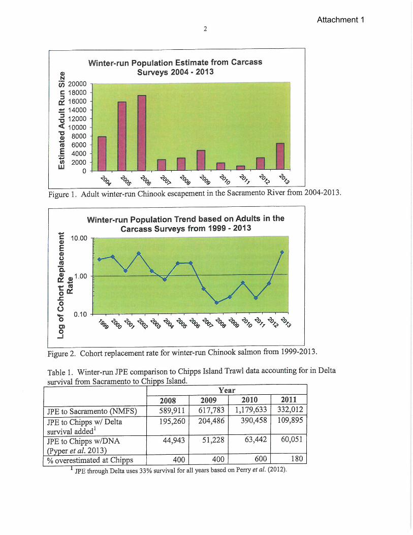
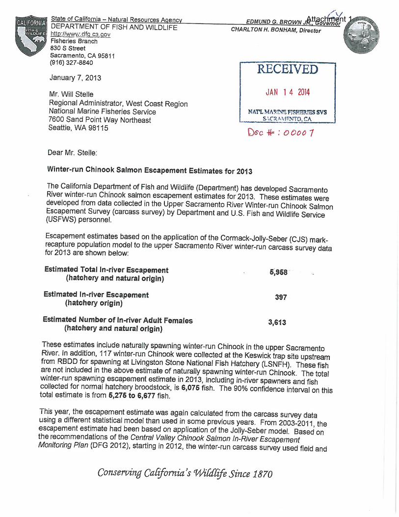
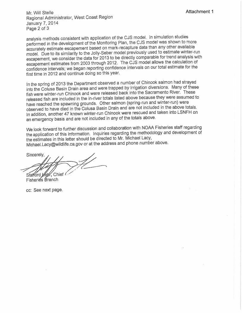
1. Escapement: Adult spawners are estimated from annual carcass counts using mark-recapture data conducted in the upper Sacramento River from the end of May to the beginning of September. Typically, peak spawning occurs in July. The official estimate of escapement is prepared by CDFW (see enclosure 1 in Attachment 1). The estimate is based on the application of the Cormack Jolly-Seber (CJS) model with the addition of 90 percent confidence intervals. It estimates the total number of naturally spawning in-river winter-run Chinook salmon, including hatchery returns, and those taken in for broodstock at the Livingston Stone National Fish Hatchery (LSNFH). Beginning in 2009, LSNFH stopped taking hatchery-origin spawners for its broodstock to reduce genetic drift, and now uses only natural fish (non-clipped) for its broodstock collection. The sex ratio in the CJS model is based on winter-run captured in the trap at the base of Keswick Dam for LSNFH broodstock. From the CDFW official estimate of escapement, NMFS obtains the estimated number of naturally-spawning females to use in the JPE.

2. Pre-spawn mortality: This is the number of females that die before spawning. It is estimated from observations made during the carcass counts. Typically, this number represents 1-2 percent of the total number of females.

3. Temperature impacts: The impact of high water temperatures is factored in to total production by calculating the percent redds observed below the temperature compliance point for that year and applying it to the number of eggs produced. For the JPE, NMFS assumes 100 percent mortality for any redds constructed downstream of the temperature

2  

compliance point. In reality, mortality would vary depending on the degree of exposure. Egg loss due to high water temperatures (greater than daily average of 56 ºF) is typically less than 0.5% of the total eggs produced in most years (~1-2 redds below the temperature compliance point).

4. Fecundity: This is the number of eggs per female spawner. Prior to 2000, NMFS used values for fecundity derived from the literature or female length regressions (e.g., 3,800 eggs/female). More recently, the value is obtained from an average of eggs per females spawned at LSNFH (typically, n <50). The number of eggs depends on female size, but ranges from 4,000–5,800 eggs/female. The average over the last 5 years (2009–2013) has been 4,925 eggs/female (Rueth 2013).

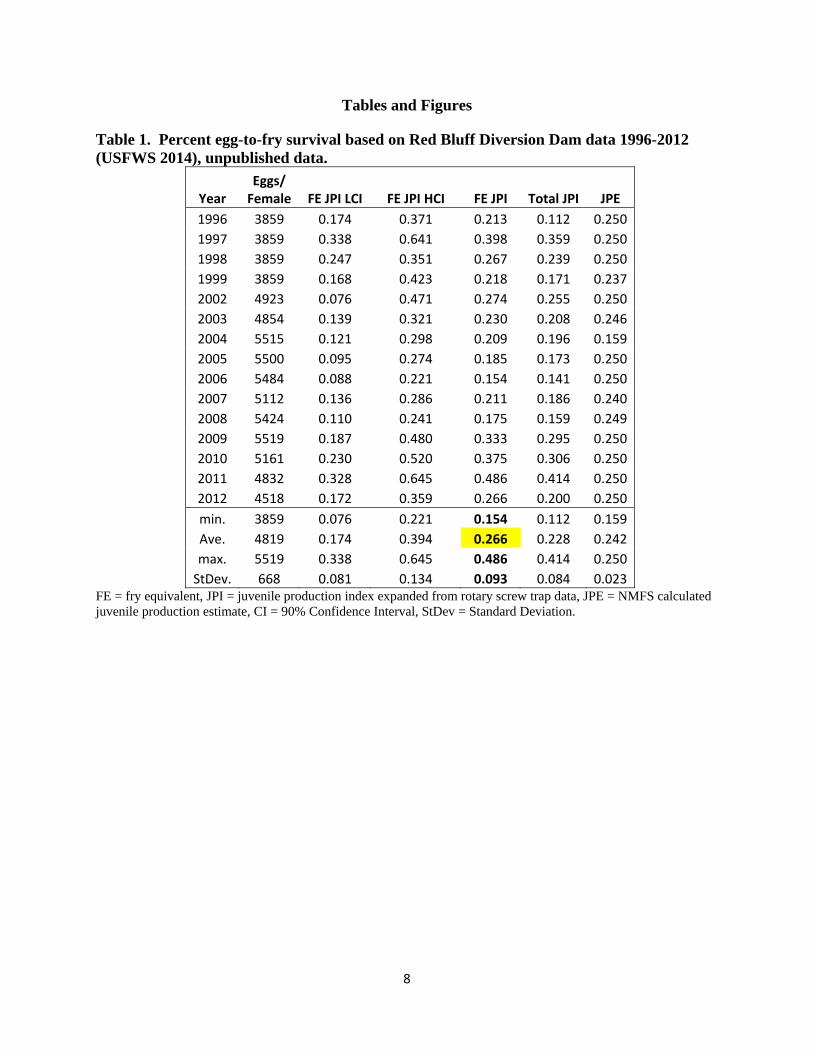
5. Survival (egg-to-fry): This is the first of 3 survival terms used to describe different juvenile life stages. It covers the time from when the eggs are laid to when fry leave the spawning gravel and begin migrating downstream past Red Bluff Diversion Dam (RBDD). In the past, this term was included in a larger term characterizing egg-to-smolt survival (S = 0.1475) derived from fall-run. However, starting in 2012, this survival term was split into egg-to-fry and fry-to-smolt survival, where egg-to-fry survival was S = 0.25 due to direct measurements of winter-run production (Table 1, Figure 1). In comparison, for the U.S. Fish and Wildlife Service’s (USFWS) juvenile production index (JPI), egg-to-fry survival was calculated based on annual data, comparing the number of juveniles estimated passing RBDD (based on expansion from rotary screw trap sampling) to the number of females estimated in the carcass surveys to determine average survival to the fry stage (Table 1).

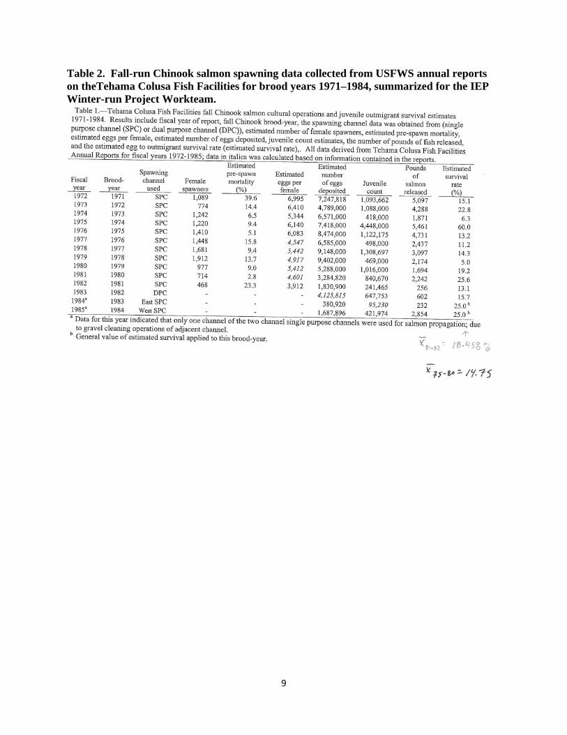
6. Survival (fry-to-smolt): The second survival term describes fry-to-smolt survival (S=0.59), which includes parr and pre-smolt life stages. Pre-smolts are used in calculating the number of fry equivalents passing RBDD (Poytress and Carrillo 2012), since not all winter-run are the same size when they begin migrating downstream. In 2012, this survival term was added after review by the Winter-run Project Work Team to describe juvenile growth and emigration for the 3-6 months spent holding in the upper Sacramento River (i.e., Red Bluff to Colusa). Previously, S=0.1475 was used as a combined egg-to-smolt survival term in the JPE to describe egg-to-smolt survival (i.e., 0.25 x 0.59 = 0.1475) based on the average fall-run Chinook survival rates obtained from the Tehama-Colusa Spawning Channel 1971–1984 (Table 2).

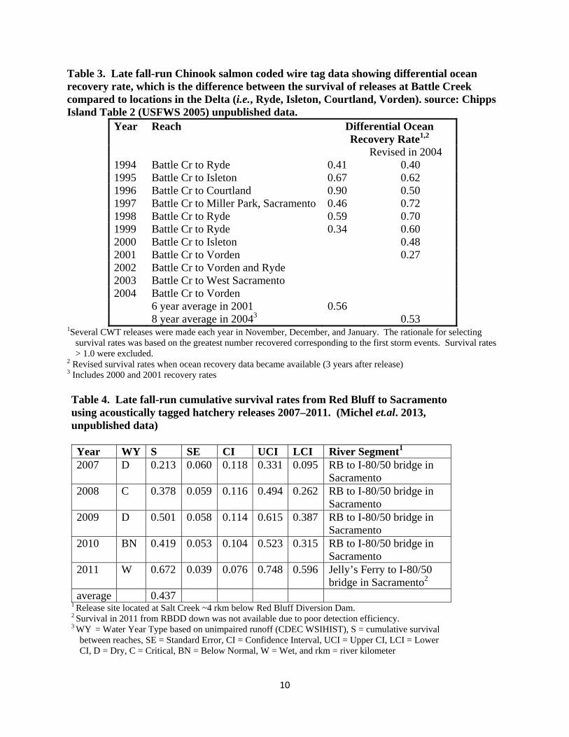
7. Survival (smolt-to-Delta): The third survival term describes survival from the smolt stage to the Delta (S = 0.53). Although the exact location in the Sacramento River that winter-run become smolts is unknown, for the JPE, this term describes downstream emigration from approximately Colusa to the time they enter the Delta (defined as Sacramento, or start of the legal Delta). This term was based on the difference in survival rates between paired coded wire tag (CWT) releases, using late fall-run Chinook as surrogates, between Battle Creek in the upper Sacramento River above RBDD, and Ryde located in the Delta (USFWS 2005, Table 3). Using ocean recoveries of the CWTs, the difference in survival between the two locations gave an approximate survival rate for in-river life-stages. These data were then updated as subsequent years became available and

3  

represents an average of 8 years, from 1994–2001. Data from 2002–2004 were not included because tag returns were not available. After 2004, the USFWS stopped making paired releases using CWTs due to funding restraints, concern about straying impacts, and the rising use of acoustic tags.1

8. Confidence Intervals (CIs): The need to recognize uncertainty in the JPE was a key component of early reviews (Brown and Kimmerer 2002). The application of confidence intervals to the JPE began in 2009 when NMFS contracted Cramer Fish Sciences (CFS) to develop a model that would incorporate CIs based on the best data available. The CFS model (CFS 2010) uses a GoldSim dashboard application with the following input data: (1) number of winter-run carcasses per day, (2) number of females, (3) daily average water temperatures, and (4) daily flow data from CDEC at Freeport. The CFS model fits a standard Ricker stock-recruitment curve to determine the number of fry produced using both carcass and RBDD data. Daily carcass data were used to determine egg deposition in time. A generalized additive model was used to fit non-linear temperature and survival data (CFS 2010). The default survival to the Delta was based on late fall-un CWT releases (S= 0.53) used in the winter-run JPE. The data for each year can be changed (e.g., temperature, survival, water year type, river flows, etc.).

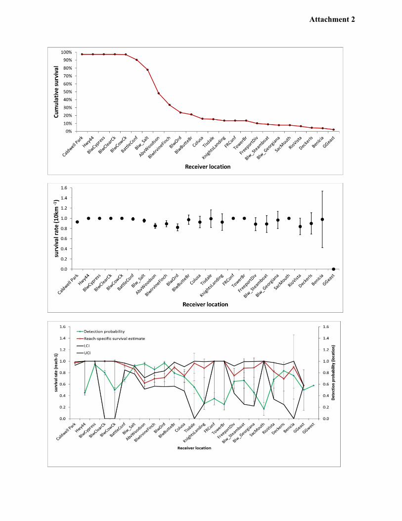
A. Recent Data from Acoustically-tagged Releases From November 2013 through January 2014, the Winter-run Project Work Team (WRPWT), under the Interagency Ecological Program, began a review of the JPE to assess the use of acoustic tag data on juvenile Chinook salmon releases in the upper Sacramento River. At the time most of these data were unpublished. A subteam of the WRPWT was formed to analyze the available acoustic data and compare them to the existing survival rates based on CWT data (attachments 2-4). Individual researchers were contacted for data (Figures 2-4). Reach survival from Red Bluff to Sacramento was compared between releases. In all, there were 6 years in which acoustic tag releases were made; 5 years using late fall-run, and 1 year using winter-run. The acoustic tag data showed significant differences in run timing and survival rates between the late fall-run releases and the winter-run release (attachment 2). In 2013, juvenile winter-run spent considerable time (from 30-50 days) holding in the upper Sacramento River as compared to the late fall-run releases that left the upper river immediately (Figure 2). In addition, when compared to average late fall-run survival (S=0.43), winter-run survival (S=0.15) was much lower between Red Bluff and Sacramento (see below).

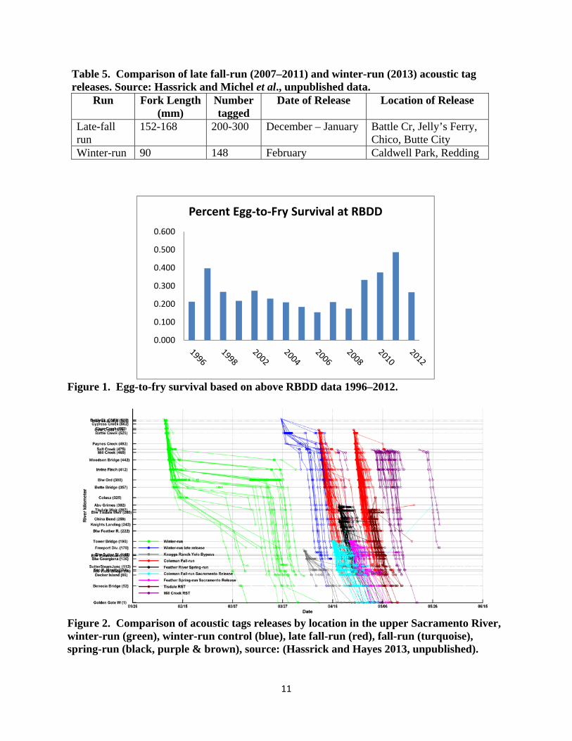
1. Late fall-run Chinook salmon: The average survival rate from Salt Creek (located at RM 240, approximately 2.5 river miles downstream of RBDD) to Sacramento (measured at the I-80/Hwy 50 bridge) for the five releases from 2007– 2011 was S=0.437 (Table 4). In comparison, the JPE uses S= 0.53 based on CWT data from late fall-run ocean recoveries. The 2007–2011 water years were all classified as dry, except for 2011, which was classified as a wet year with subsequently higher survival in that year (Figures 3-4).

                                                            1 For more information on these studies, see USFWS, Anadromous Fisheries Restoration Program/Delta Action 8, http://www.fws.gov/stockton/jfmp.  

4  

2. Winter-run Chinook salmon: 2013 was the first year direct measurements of winter-run survival became available using acoustic tag data. 148 hatchery winter-run were tagged and released in February near Caldwell Park (RM 299) in Redding. A later release of 48 control fish was made in March. The survival rate for the February release was S=0.156 (95% LCI=0.104, UCI=0.228) from Salt Creek to the Tower Bridge in Sacramento (Hassrick and Hayes 2013). Survival to the Delta was considerably lower than the 5 years of late fall-run acoustic tag releases, and lower than the previously-used survival rates in the JPE based on CWT data.

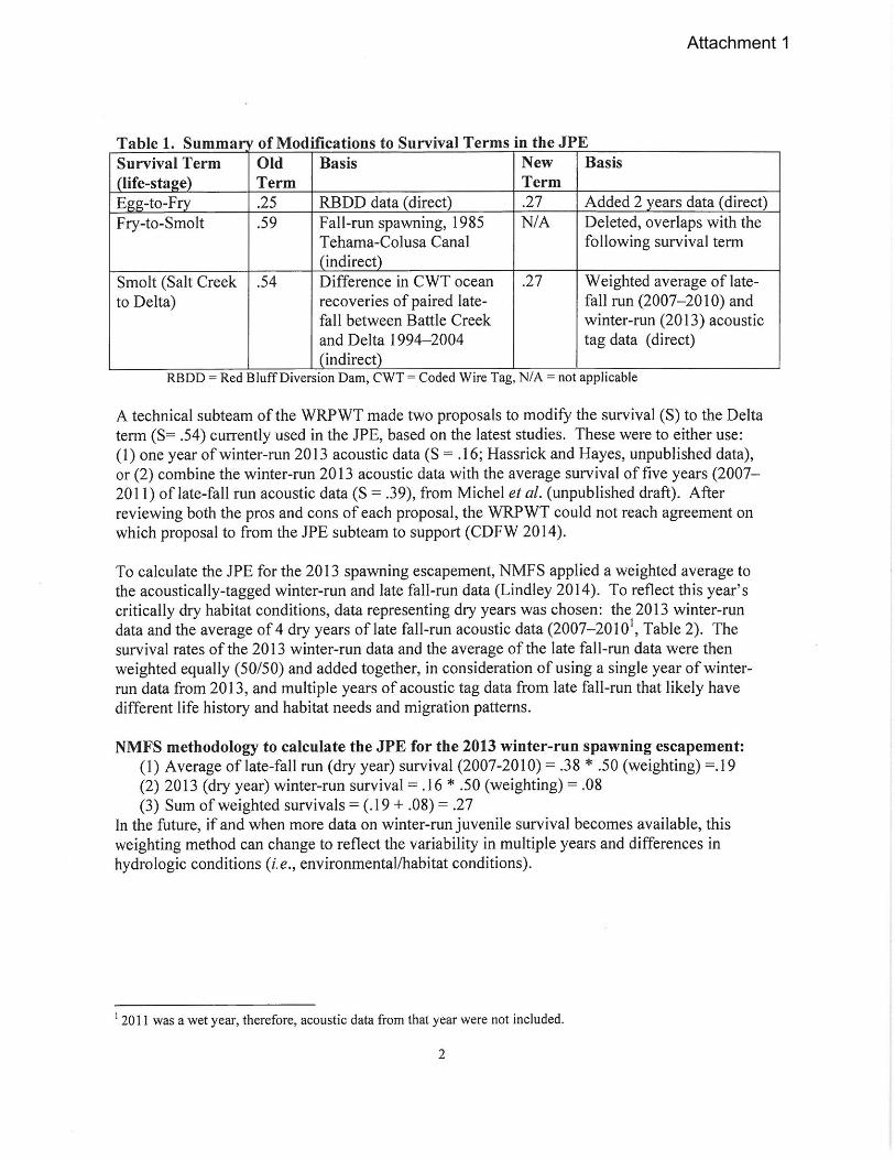
The subteam performed a number of analyses to determine survival rates to the Delta. It reviewed the current JPE methodology using Chipps Island ocean recoveries (CWTs) data up to 2011 (USFWS 2013). It reviewed the latest winter-run and late fall-run acoustic tag releases (Tables 4 and 5). Then it reviewed the latest trawl data from Chipps Island based on genetic identification (Pyper et al. 2013). The subteam back-calculated the different survival rates from acoustic tag and CWT data from RBDD to Chipps Island, minus through Delta survival (i.e., Sacramento to Chipps Island), to determine juvenile production estimates that were close to estimates based on observed genetic identification. The subteam recommended the following changes to the survival terms, along with pros and cons (attachment 4).

1. use of the 2013 winter-run acoustic tag survival (16%); 2. or, combine the 5-year average of late fall-run (2007-2011) and 2013 winter-run acoustic

data (39%); 3. apply 2 significant figures to survival terms; and 4. change egg-to-fry survival from 25% to 27% based on added 2 years of additional data.

The WRPWT provided a memorandum back to the subteam (attachment 5). Although the WRPWT could not reach consensus on which survival rate to use, it did agree that the use of data from acoustic tags rather than surrogate releases (i.e., CWT’ed late fall-run) provided direct information on the unique behaviors and life histories of the winter-run population instead of requiring additional inferences.  

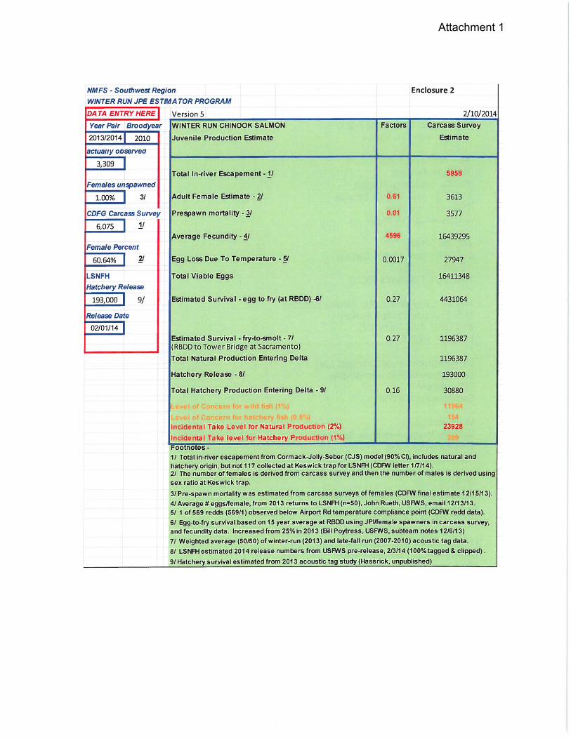
B. Application of Acoustic tag data After reviewing the WRPWT subteam analysis and options for consideration to estimate winter-run survival, NMFS conferred with its Southwest Fisheries Science Center on the appropriate data to use for the JPE. NMFS concluded that there was enough information to modify the JPE methodology using acoustic tag data (enclosure 3 in Attachment 1). The following changes were applied by NMFS to the winter-run JPE for broodyear 2013:

1. Egg-to-fry survival changed from 0.25 to 0.27 based on 2 years additional data from RBDD.

2. The previous fry-to-smolt and smolt-to-Delta survival terms were combined together using a combination of acoustic tag data from winter-run and late fall-run releases (Michel et. al. unpublished). This term would a more direct measure of survival and eliminate overlap between survival terms.

3. A 50 percent weighting factor was applied to the late fall-run and winter-run acoustic tag survival data to account for the one year of data from winter-run.

5  

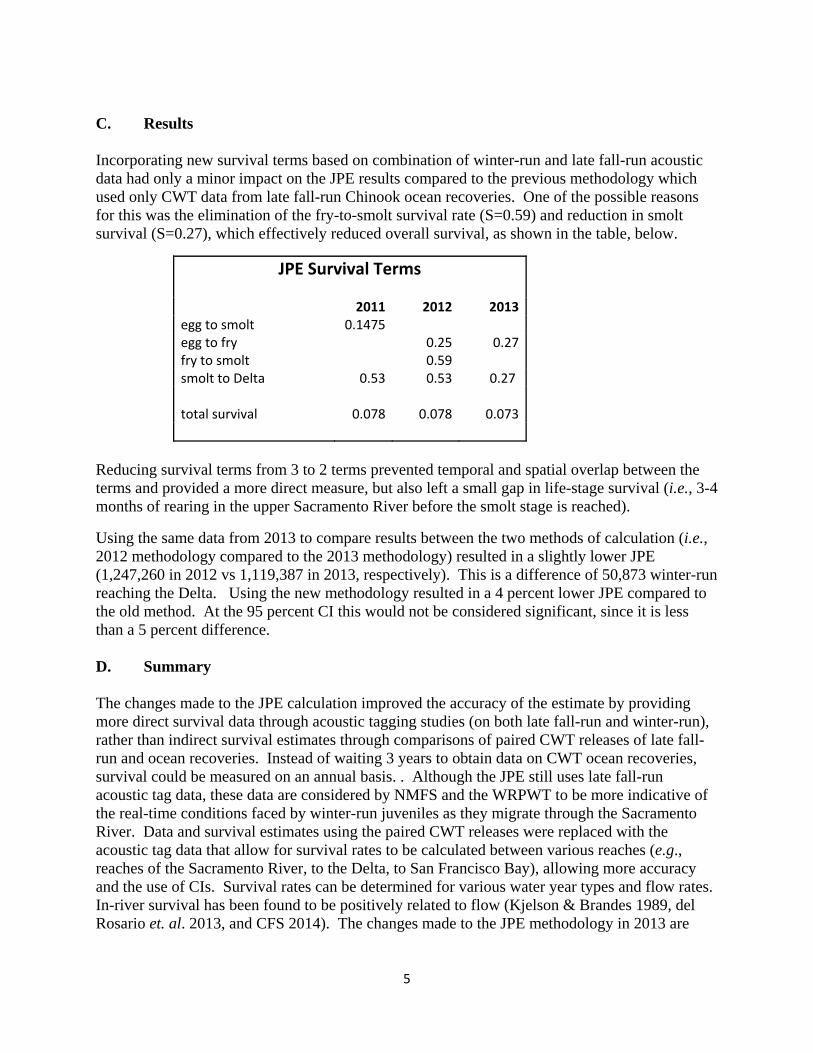
C. Results Incorporating new survival terms based on combination of winter-run and late fall-run acoustic data had only a minor impact on the JPE results compared to the previous methodology which used only CWT data from late fall-run Chinook ocean recoveries. One of the possible reasons for this was the elimination of the fry-to-smolt survival rate (S=0.59) and reduction in smolt survival (S=0.27), which effectively reduced overall survival, as shown in the table, below. 

JPE Survival Terms      2011 2012 2013egg to smolt  0.1475   egg to fry  0.25 0.27fry to smolt  0.59smolt to Delta  0.53 0.53        0.27 

total survival  0.078 0.078 0.073 

Reducing survival terms from 3 to 2 terms prevented temporal and spatial overlap between the terms and provided a more direct measure, but also left a small gap in life-stage survival (i.e., 3-4 months of rearing in the upper Sacramento River before the smolt stage is reached).

Using the same data from 2013 to compare results between the two methods of calculation (i.e., 2012 methodology compared to the 2013 methodology) resulted in a slightly lower JPE (1,247,260 in 2012 vs 1,119,387 in 2013, respectively). This is a difference of 50,873 winter-run reaching the Delta. Using the new methodology resulted in a 4 percent lower JPE compared to the old method. At the 95 percent CI this would not be considered significant, since it is less than a 5 percent difference. D. Summary

The changes made to the JPE calculation improved the accuracy of the estimate by providing more direct survival data through acoustic tagging studies (on both late fall-run and winter-run), rather than indirect survival estimates through comparisons of paired CWT releases of late fall-run and ocean recoveries. Instead of waiting 3 years to obtain data on CWT ocean recoveries, survival could be measured on an annual basis. . Although the JPE still uses late fall-run acoustic tag data, these data are considered by NMFS and the WRPWT to be more indicative of the real-time conditions faced by winter-run juveniles as they migrate through the Sacramento River. Data and survival estimates using the paired CWT releases were replaced with the acoustic tag data that allow for survival rates to be calculated between various reaches (e.g., reaches of the Sacramento River, to the Delta, to San Francisco Bay), allowing more accuracy and the use of CIs. Survival rates can be determined for various water year types and flow rates. In-river survival has been found to be positively related to flow (Kjelson & Brandes 1989, del Rosario et. al. 2013, and CFS 2014). The changes made to the JPE methodology in 2013 are

6  

consistent with improvements that have been made in the past (e.g., change to carcass surveys in 2000, change to CIs in 2004) as a result of WRPWT review and analysis.

E. Questions for Review Panel

1. How important is it to eliminate overlap in survival terms, vs. potentially not including the survival rate of the fry life history stage?

2. How should the missing life-stages (i.e., fry-to-smolt) and the gap in juvenile rearing from RBDD to Salt Creek be accounted for in the current JPE methodology?

3. Hatchery origin juvenile winter-run have shown a unique life-history strategy not seen in other runs, in that they hold upstream in dry years for 30-50 days. How should this behavior be incorporated into the JPE?

4. The weighting for the JPE in 2013 was 50% for the 5 years of late fall-run acoustic tag data, and 50% for the one year of winter-run acoustic tag data.

a. The late fall-run acoustic tag data included data from various water year types, and the year of winter-run acoustic tag survival was conducted in a dry water year. How should water year type be considered and factored into the weighting in any given water year?

b. What should the weighting be between late fall-run and winter-run acoustic tag data with each additional year of winter-run acoustic tag data? At what point (how many years of winter-run acoustic tag data) should we not consider the late fall-run acoustic tag data to develop the winter-run JPE?

5. What additional studies or methods would you recommend to improve the accuracy of

the JPE in the future?

6. Given that approximately 4.43 million fry were estimated to pass RBDD from the JPE calculator, but only 1.78 million fry were estimated to pass RBDD based on U.S. Fish and Wildlife Service’s rotary screw trapping, how should these conflicting data be interpreted?

F. References

Brown, R. and W. Kimmerer. 2002. Chinook Salmon and the Environmental Water Account: A Summary of the 2002 Salmonid Workshop. Prepared for the CALFED Science Program, October 2002, Sacramento, CA. 47 pg.

CFS (Cramer Fish Sciences) 2014. A Revised Sacramento River Winter Chinook Salmon Juvenile Production Model. Prepared by Kristopher Jones, Paul Bergman, and Brad Cavallo for the National Oceanic and Atmospheric Administration, Sacramento, CA. 21 pg.

7  

del Rosario, R. B, Y. J. Redler, K. Newman, P. L. Brandes, T. Sommer, K. Reece, and R. Vincik. 2013. Migration Patterns of Juvenile Winter-Run-Sized Chinook Salmon (Oncorhynchus tshawytscha) through the Sacramento–San Joaquin Delta. San Francisco Estuary & Watershed Science 11(1): 1-22.

Hassrick, J. and S. Hayes. 2013. Survival of Migratory Patterns of Juvenile Winter-run Chinook

salmon in the Sacramento River, Delta, and S.F. Bay. Unpublished results of first year acoustic tag study. NOAA, UCD, CFS, DWR, and USFWS.

Kjelson, M.A. and P.L. Brandes. 1989. The use of smolt estimates to quantify the effects if

habitat changes on salmonid stocks in the Sacramento-San Joaquin Rivers, California. Pages 100-115 in C.D. Levings, L.B. Holtby, and M.A. Henderson (editors), Proceedings of the National Workshop on Effects of Habitat Alteration on Salmonid Stocks. Canadian Special Publications of Fisheries and Aquatic Sciences 105.

Poytress, W. R. and F. D. Carrillo. 2012. Brood-Year 2010 Winter Chinook Juvenile Production

Indices with Comparisions to Juvenile Production Estimates Derived from Adult Escapement. Report of U.S. Fish and Wildlife Service to California Department of Fish and Game and U.S. Bureau of Reclamation. U.S. Fish and Wildlife Service, 42 pp.

8  

Tables and Figures

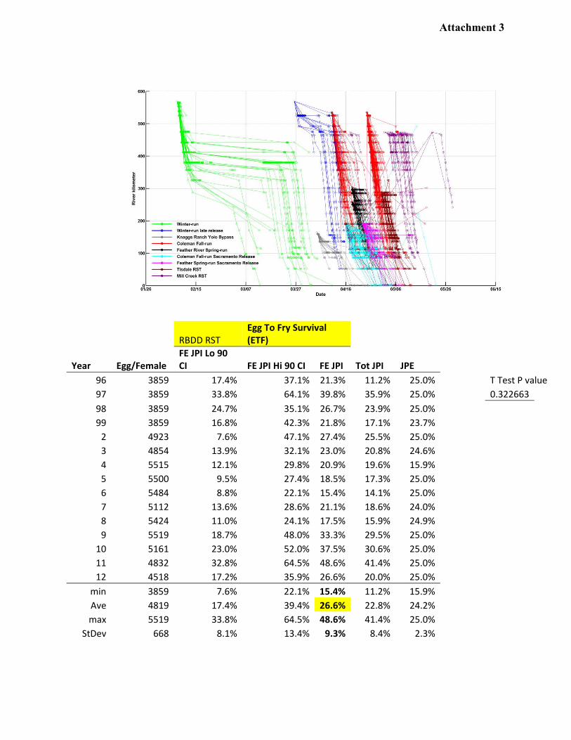
Table 1. Percent egg-to-fry survival based on Red Bluff Diversion Dam data 1996-2012 (USFWS 2014), unpublished data.

Year Eggs/ Female  FE JPI LCI  FE JPI HCI  FE JPI  Total JPI  JPE 

1996  3859  0.174  0.371  0.213  0.112  0.250 

1997  3859  0.338  0.641  0.398  0.359  0.250 

1998  3859  0.247  0.351  0.267  0.239  0.250 

1999  3859  0.168  0.423  0.218  0.171  0.237 

2002  4923  0.076  0.471  0.274  0.255  0.250 

2003  4854  0.139  0.321  0.230  0.208  0.246 

2004  5515  0.121  0.298  0.209  0.196  0.159 

2005  5500  0.095  0.274  0.185  0.173  0.250 

2006  5484  0.088  0.221  0.154  0.141  0.250 

2007  5112  0.136  0.286  0.211  0.186  0.240 

2008  5424  0.110  0.241  0.175  0.159  0.249 

2009  5519  0.187  0.480  0.333  0.295  0.250 

2010  5161  0.230  0.520  0.375  0.306  0.250 

2011  4832  0.328  0.645  0.486  0.414  0.250 

2012  4518  0.172  0.359  0.266  0.200  0.250 

min.  3859  0.076  0.221  0.154  0.112  0.159 

Ave.  4819  0.174  0.394  0.266  0.228  0.242 

max.  5519  0.338  0.645  0.486  0.414  0.250 

StDev.  668  0.081  0.134  0.093  0.084  0.023 FE = fry equivalent, JPI = juvenile production index expanded from rotary screw trap data, JPE = NMFS calculated juvenile production estimate, CI = 90% Confidence Interval, StDev = Standard Deviation.

9  

Table 2. Fall-run Chinook salmon spawning data collected from USFWS annual reports on theTehama Colusa Fish Facilities for brood years 1971–1984, summarized for the IEP Winter-run Project Workteam.

10  

Table 3. Late fall-run Chinook salmon coded wire tag data showing differential ocean recovery rate, which is the difference between the survival of releases at Battle Creek compared to locations in the Delta (i.e., Ryde, Isleton, Courtland, Vorden). source: Chipps Island Table 2 (USFWS 2005) unpublished data.

Year Reach Differential Ocean Recovery Rate1,2

Revised in 2004 1994 Battle Cr to Ryde 0.41 0.40 1995 Battle Cr to Isleton 0.67 0.62 1996 Battle Cr to Courtland 0.90 0.50 1997 Battle Cr to Miller Park, Sacramento 0.46 0.72 1998 Battle Cr to Ryde 0.59 0.70 1999 Battle Cr to Ryde 0.34 0.60 2000 Battle Cr to Isleton 0.48 2001 Battle Cr to Vorden 0.27 2002 Battle Cr to Vorden and Ryde 2003 Battle Cr to West Sacramento 2004 Battle Cr to Vorden 6 year average in 2001 0.56 8 year average in 20043 0.53

1Several CWT releases were made each year in November, December, and January. The rationale for selecting survival rates was based on the greatest number recovered corresponding to the first storm events. Survival rates > 1.0 were excluded.

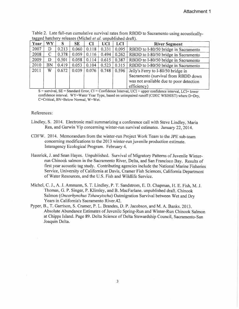
2 Revised survival rates when ocean recovery data became available (3 years after release) 3 Includes 2000 and 2001 recovery rates Table 4. Late fall-run cumulative survival rates from Red Bluff to Sacramento using acoustically tagged hatchery releases 2007–2011. (Michel et.al. 2013, unpublished data)

Year WY S SE CI UCI LCI River Segment1

2007 D 0.213 0.060 0.118 0.331 0.095 RB to I-80/50 bridge in Sacramento

2008 C 0.378 0.059 0.116 0.494 0.262 RB to I-80/50 bridge in Sacramento

2009 D 0.501 0.058 0.114 0.615 0.387 RB to I-80/50 bridge in Sacramento

2010 BN 0.419 0.053 0.104 0.523 0.315 RB to I-80/50 bridge in Sacramento

2011 W 0.672 0.039 0.076 0.748 0.596 Jelly’s Ferry to I-80/50 bridge in Sacramento2

average 0.437 1 Release site located at Salt Creek ~4 rkm below Red Bluff Diversion Dam. 2 Survival in 2011 from RBDD down was not available due to poor detection efficiency. 3 WY = Water Year Type based on unimpaired runoff (CDEC WSIHIST), S = cumulative survival

between reaches, SE = Standard Error, CI = Confidence Interval, UCI = Upper CI, LCI = Lower CI, D = Dry, C = Critical, BN = Below Normal, W = Wet, and rkm = river kilometer

11  

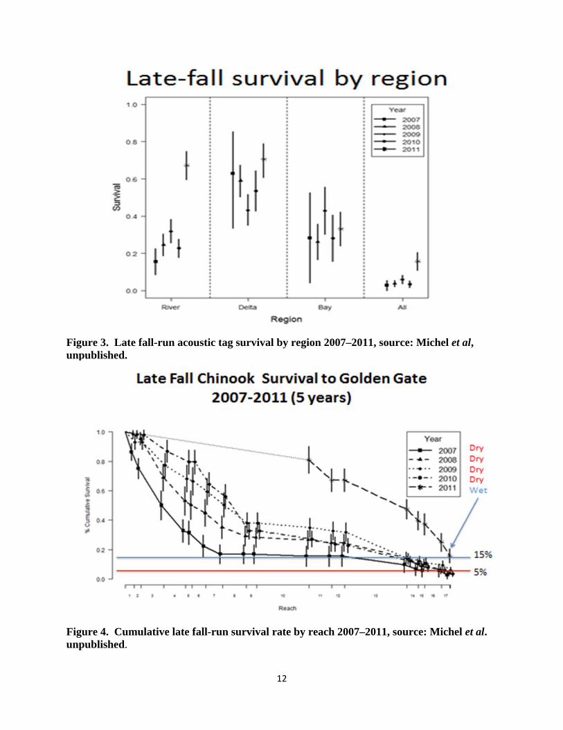
Table 5. Comparison of late fall-run (2007–2011) and winter-run (2013) acoustic tag releases. Source: Hassrick and Michel et al., unpublished data.

Run Fork Length (mm)

Number tagged

Date of Release Location of Release

Late-fall run

152-168 200-300 December – January Battle Cr, Jelly’s Ferry, Chico, Butte City

Winter-run 90 148 February Caldwell Park, Redding

Figure 1. Egg-to-fry survival based on above RBDD data 1996–2012.

Figure 2. Comparison of acoustic tags releases by location in the upper Sacramento River, winter-run (green), winter-run control (blue), late fall-run (red), fall-run (turquoise), spring-run (black, purple & brown), source: (Hassrick and Hayes 2013, unpublished).

0.000

0.100

0.200

0.300

0.400

0.500

0.600

Percent Egg‐to‐Fry Survival at RBDD

12  

Figure 3. Late fall-run acoustic tag survival by region 2007–2011, source: Michel et al, unpublished.

Figure 4. Cumulative late fall-run survival rate by reach 2007–2011, source: Michel et al. unpublished. 

13  

Attachments: 1. February 21, 2014, letter from NMFS to Reclamation transmitting the JPE 2. WRPWT subteam notes: November 26, 2013 3. WRPWT subteam notes: December 6, 2013 4. WRPWT subteam notes: December 19, 2013 5. Memorandum from the Winter-run Project Work Team to its subteam concerning

the subteam summary report of the Juvenile Production Estimate. Interagency Ecological Program, Winter-run Project Work Team. January 31, 2014. 2 pg.

Attachment 1

Attachment 1

Attachment 1

Attachment 1

Attachment 1

Attachment 1

Attachment 1

Attachment 1

Attachment 1

Attachment 1

Attachment 1

Attachment 1

Attachment 1

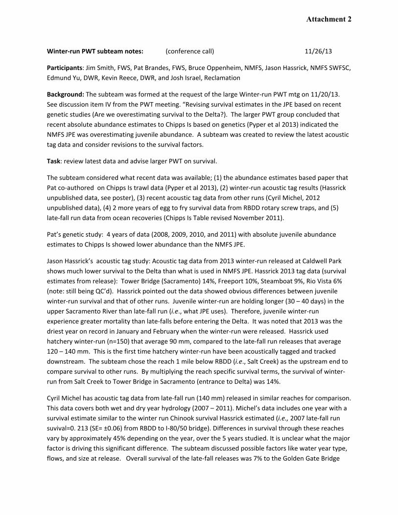
Winter‐run PWT subteam notes:   (conference call)        11/26/13 

Participants: Jim Smith, FWS, Pat Brandes, FWS, Bruce Oppenheim, NMFS, Jason Hassrick, NMFS SWFSC, 

Edmund Yu, DWR, Kevin Reece, DWR, and Josh Israel, Reclamation 

Background: The subteam was formed at the request of the large Winter‐run PWT mtg on 11/20/13.  

See discussion item IV from the PWT meeting. “Revising survival estimates in the JPE based on recent 

genetic studies (Are we overestimating survival to the Delta?).  The larger PWT group concluded that 

recent absolute abundance estimates to Chipps Is based on genetics (Pyper et al 2013) indicated the 

NMFS JPE was overestimating juvenile abundance.  A subteam was created to review the latest acoustic 

tag data and consider revisions to the survival factors. 

Task: review latest data and advise larger PWT on survival. 

The subteam considered what recent data was available; (1) the abundance estimates based paper that 

Pat co‐authored  on Chipps Is trawl data (Pyper et al 2013), (2) winter‐run acoustic tag results (Hassrick 

unpublished data, see poster), (3) recent acoustic tag data from other runs (Cyril Michel, 2012 

unpublished data), (4) 2 more years of egg to fry survival data from RBDD rotary screw traps, and (5) 

late‐fall run data from ocean recoveries (Chipps Is Table revised November 2011). 

Pat’s genetic study:  4 years of data (2008, 2009, 2010, and 2011) with absolute juvenile abundance 

estimates to Chipps Is showed lower abundance than the NMFS JPE.   

Jason Hassrick’s  acoustic tag study: Acoustic tag data from 2013 winter‐run released at Caldwell Park 

shows much lower survival to the Delta than what is used in NMFS JPE. Hassrick 2013 tag data (survival 

estimates from release):  Tower Bridge (Sacramento) 14%, Freeport 10%, Steamboat 9%, Rio Vista 6% 

(note: still being QC’d).  Hassrick pointed out the data showed obvious differences between juvenile 

winter‐run survival and that of other runs.  Juvenile winter‐run are holding longer (30 – 40 days) in the 

upper Sacramento River than late‐fall run (i.e., what JPE uses).  Therefore, juvenile winter‐run 

experience greater mortality than late‐falls before entering the Delta.  It was noted that 2013 was the 

driest year on record in January and February when the winter‐run were released.  Hassrick used 

hatchery winter‐run (n=150) that average 90 mm, compared to the late‐fall run releases that average 

120 – 140 mm.  This is the first time hatchery winter‐run have been acoustically tagged and tracked 

downstream.  The subteam chose the reach 1 mile below RBDD (i.e., Salt Creek) as the upstream end to 

compare survival to other runs.  By multiplying the reach specific survival terms, the survival of winter‐

run from Salt Creek to Tower Bridge in Sacramento (entrance to Delta) was 14%. 

Cyril Michel has acoustic tag data from late‐fall run (140 mm) released in similar reaches for comparison.  

This data covers both wet and dry year hydrology (2007 – 2011). Michel’s data includes one year with a 

survival estimate similar to the winter run Chinook survival Hassrick estimated (i.e., 2007 late‐fall run 

suvival=0. 213 (SE= ±0.06) from RBDD to I‐80/50 bridge). Differences in survival through these reaches 

vary by approximately 45% depending on the year, over the 5 years studied. It is unclear what the major 

factor is driving this significant difference.  The subteam discussed possible factors like water year type, 

flows, and size at release.   Overall survival of the late‐fall releases was 7% to the Golden Gate Bridge 

Attachment 2

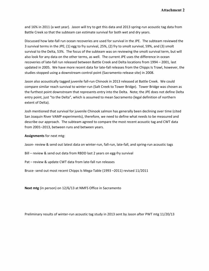
and 16% in 2011 (a wet year).  Jason will try to get this data and 2013 spring‐run acoustic tag data from 

Battle Creek so that the subteam can estimate survival for both wet and dry years.  

Discussed how late‐fall run ocean recoveries are used for survival in the JPE.  The subteam reviewed the 

3 survival terms in the JPE; (1) egg to fry survival, 25%, (2) fry to smolt survival, 59%, and (3) smolt 

survival to the Delta, 53%.  The focus of the subteam was on reviewing the smolt survival term, but will 

also look for any data on the other terms, as well.  The current JPE uses the difference in ocean 

recoveries of late‐fall run released between Battle Creek and Delta locations from 1994 – 2001, last 

updated in 2005.  We have more recent data for late‐fall releases from the Chipps Is Trawl, however, the 

studies stopped using a downstream control point (Sacramento release site) in 2008.  

Jason also acoustically tagged juvenile fall‐run Chinook in 2013 released at Battle Creek.  We could 

compare similar reach survival to winter‐run (Salt Creek to Tower Bridge).  Tower Bridge was chosen as 

the furthest point downstream that represents entry into the Delta.  Note; the JPE does not define Delta 

entry point, just “to the Delta”, which is assumed to mean Sacramento (legal definition of northern 

extent of Delta). 

Josh mentioned that survival for juvenile Chinook salmon has generally been declining over time (cited 

San Joaquin River VAMP experiments), therefore, we need to define what needs to be measured and 

describe our approach.  The subteam agreed to compare the most recent acoustic tag and CWT data 

from 2001–2013, between runs and between years. 

Assignments for next mtg: 

Jason‐ review & send out latest data on winter‐run, fall‐run, late‐fall, and spring‐run acoustic tags  

Bill – review & send out data from RBDD last 2 years on egg‐fry survival  

Pat – review & update CWT data from late‐fall run releases 

Bruce‐ send out most recent Chipps Is Mega‐Table (1993 –2011) revised 11/2011 

 

Next mtg (in person) on 12/6/13 at NMFS Office in Sacramento 

 

 

Preliminary results of winter‐run acoustic tag study in 2013 sent by Jason after PWT mtg 11/20/13 

Attachment 2

 

 

 

Attachment 2

Winter‐run Subteam Mtg (in person, NMFS Office Sacramento)        12/6/13 

Participants: Bruce Oppenheim, NMFS, Jason Hassrick, NMFS, Pat Brandes, FWS, Jim Smith, FWS, Bill 

Poytress, FWS, Josh Israel, Reclamation, Edmund Yu, DWR, Kevin Reece, DWR. 

Agenda: A) Review recent CWT and acoustic data on winter‐run 

   B) Review and revise survival terms in JPE based on recent data 

Started with the review of the Chipps Is ocean recoveries (CWTs) data up to 2011 (see Chipps Is Table 

1993‐2011) because that is what is currently used in the NMFS JPE.  Pat presented her analysis of data 

on survival based on paired hatchery late‐fall run releases from Battle Creek and an associated Delta 

location (e.g., Courtland, Sac, Ryde, Isleton) up to 2008. The data suffers from high variability, 

uncertainty in recapture efforts, and only yields an indirect measurement of survival. In some years, 

values are used as averages of releases, in other years a single value is used based on timing of release 

with storms or flow increases. In other years, biologists decided not to use any results since values > 1.0, 

suggesting the assumptions regarding recapture rates are not statistically valid.  No data for 2012 and 

2013 late‐fall releases yet, because they have not shown up in ocean harvest.  This limits use of most 

recent data for comparison, always 3 years behind.  However, FWS has not been conducting paired late‐

fall run Chinook salmon releases since about 2008. The subteam consensus was not to use this data due 

to the problems inherit in sampling, it results in an indirect measure of what we are attempting to 

capture in the term, and because of perceived differences in behavior between late‐fall and winter‐run 

emigration.  The subteam felt that there were better data available now in the more recent acoustic tag 

studies. 

Then reviewed the Hassrick 2013 winter‐run acoustic data (n=148).  Two releases were made, one in 

February with the normal hatchery release, and one later in March.   Jason presented the unpublished 

results of his study.  Livingston Stone National Fish Hatchery does one release a year (unlike Coleman), 

so the tagged 148 fish (shown in green) were released on February 7 with that group from Caldwell 

Park.  An additional 25 smolts (shown in blue) were retained to assess tag effects and released on March 

24th.  This is notable because even the later released fish held in the upper river before migrating 

downstream.  No other runs showed this behavior for this year.  This data included reach survival from 

Caldwell Park (Redding to the Golden Gate).   

One concern is that the results only represent one year, and it was the driest year on record.  Another 

concern was the limited sample size and detection probabilities used to estimate survival to Tower 

(n=19 being observed downstream of Tower, 5 being observed at Tower). Recent work on winter‐run 

emigration patterns, Rosario et al (2013), showed a different pattern between wet years and dry years.  

In dry years winter‐run hold in the upper river for 30–40 days, and  this pattern is captured in the 

migration timing of the 2013 acoustically tagged winter run which spent approximately  30‐50 days in 

the between Red Bluff and Colusa. In wet years, winter‐run move downstream quickly and rear in the 

Delta for 30–40 days.  The JPE only considers in‐river survival and not the Delta survival, so should we 

consider averaging wet and dry year survival? 

Attachment 3

Josh suggested we need to change the fry to smolt survival term (.59) because it was based on outdated 

fall‐run data from 1972–1981 at the Tehama‐Colusa Spawning Channel.  The fry to smolt survival term 

represents approximately 2 months in river (check old reports).  It should really represent 4 months 

from October – January.  We may need a daily mortality model for 120 days to incorporate variable 

rearing strategies in river.  Ken Newman, FWS statistician,  developed such a daily mortality model for 

the Rosario et al (2013) paper.  Pat explained the Newman model by referring to Figure 8 in the Rosario 

et al (2013).  The subteam looked at Jason’s graph of winter‐run compared to other runs (spring, fall, 

late‐fall) and concluded that winter‐run hold above Colusa for a considerable time compared to other 

runs which emigrated right out at release.  The winter‐run acoustic tag data also had a low detection 

probability (.40) between Knights Landing and Tower Bridge, but this could be due to the number of tags 

declining as they move downstream.  The standard error also increases as you move downstream.  Jason 

will look into methodology for estimating standard error.  

1st Approach: 

The subteam tried to develop a formula to account for daily mortality that could be incorporated into 

the JPE.  In particular, the subteam was interested in looking at daily mortality from Salt Creek to Colusa 

to better incorporate winter‐run rearing strategies in that reach based on a graph presented by Hassrick. 

The subteam came up with the following formula below:  

S/RKM x RKM/days = S/days  

For S/RKM, the subteam used 0.991 S/RKM, which is based on the average survival rate per km from Salt 

Creek to Colusa. For RKM/days, the subteam originally planned to use 150 RKM/40 days. Forty days was 

based on the period of 2/15 to 3/27 when winter‐run were in the Salt Creek to Colusa region (see 

Hassrick graph), while the 150 RKM represents the distance from Salt Creek to Colusa. This led to the 

following:  

(0.991 S/RKM) * (150 RKM/40 days). 

However, the above equation would give survival per 40 days and the subteam was interested in 

survival per day. To accomplish this, the subteam raised 0.991 to the 4th power and the results are below 

to capture the period of 160 days: 

(0.991^4)/4       0.991 to 4th Power = 0.964483 for 160 days 

S = 0.00238 for 4 months 

160 days represented the time period for fry to change to smolts 

S = 0.2%, In the end, the survival calculated using this approach was too low for even the Hassrick data. 

However, participants from the meeting felt this is something that would still be worth looking into as 

new ideas arise on how to determine survival per day.  

2nd Approach:   

Attachment 3

Josh proposed back‐calculating 2008–2012 data from JPI at RBDD to Chipps Is abundance estimates 

using different survival estimates (e.g., using winter‐run, spring‐run , and late‐fall acoustic data) and 

compare  to the absolute estimates made using genetics (Pyper, et al 2013).  The subteam went through 

this exercise by calculating the number entering the Delta at Sacramento based on winter‐run RBDD 

data using different survival estimates. Afterwards, the subteam compared the estimates of survival 

through the Delta, calculated by dividing the genetic estimate of winter run Chinook at Chipps by the 

number entering the Delta, to the estimated through‐delta survival reported by Perry using late‐fall 

Chinook (2007–2009 overall average survival 0.359, PWT notes). We were able to compare results from 

4 years (2008, 2009, 2010, and 2011).   

When the estimated survival to Chipps using WRC telemetry data was compared to the Perry estimates, 

the average survival estimated was very similar to the Perry estimates (Table 1).  A second modification 

using four observed years of survival from LFC releases resulted in estimated survival to Chipps that was 

an order of magnitude smaller than estimated during these years to results in the genetic estimates of 

WRC (Table 2).  An average of all acoustic releases (4 LFC +1WRC) was used for all 4 years, and resulted 

in estimated survival to Chipps that was less than half was was observed as the average Delta survival by 

Perry (Table 3).  The comparison that seemed to match estimated survival to through the Delta the best  

used the 16% survival of tagged  winter‐run Chinook from Salt Creek to Tower Bridge. 

The subteam did not reach a consensus on the best value to use, but proposed two estimates of rearing 

smolt to Delta survival; one based on the winter‐run data from 2013 (i.e., Salt Cr to Tower Bridge S =.156 

95% LCI=0.104, UCI=0.228), and the other based on late‐fall data from 2007–2011 and winter‐run data 

in 2013 (S=.39).  The subteam felt there were benefits and risks to using either survival estimate, but 

both were likely more accurate than late‐fall ocean recoveries of CWTs.  Also, some of the subteam felt 

better documentation, similar to that recently developed for the equation estimating loss at the 

facilities, should be developed with an additional section on recommendations for completing survival 

studies necessary to derive accurate estimates for calculating the JPE. There was also some discussion of 

whether the JPE calculator should continue to focus on using point estimates for survival or recommend 

completing studies documenting the relationships between survival and environmental covariates of 

interest to use in estimating JPEs.  

Arguments for and against using the WY13 winter run estimate: 

1) The winter‐run (.16) survival estimate was based on only one year of tag data in 2013 and that 

year was the driest on record.  This data should be updated every year that in‐river survival 

estimates are measured using winter run Chinook. Regardless, benefits from using this estimate 

include that it captures survival of actual winter‐run Chinook and not surrogates as in the past. 

Also, this value provides Delta survival estimates more similar to the overall average Delta 

survival based on existing genetic estimates for WRC juvenile abundance at Chipps Island (Pyper, 

et al 2013).  The back‐calculated survival estimate was similar in 3 out of 4 years (2008–2011). 

2) The late‐fall estimate (.43) survival value represents an average of both wet and dry year 

hydrology over the last 5 years (2007–2011) and includes approximately 45% variation in 

survival that may be attributed to environmental and/or experimental effects.  However, it is 

Attachment 3

not representative of winter‐run behavior.  This estimate leaves out mortality in the upper river 

due to 30–40 day known delay/rearing in winter‐run emigration and did not fit as well when 

back calculated with estimates from Chipps Is (2008–2011). 

3) A combination of late fall and winter run Chinook (0.39; 2007–2011 and 2013, respectively) 

value is inclusive of multiple species, multiple release timings, and captures low and high values 

of survival, which are anticipated to exist under different water year types and environmental 

conditions. This value is not exclusive to winter run Chinook, which is a desirable and should be 

recommended until a certain number of water year types, total release years, or some other 

measure of variation/repeatability is achieved. This value is not exclusive to releases including 

rearing smolt behavior, and there were multiple opinions about how to capture rearing survival 

in the survival values in the JPE calculator. Rearing smolt survival is incorporate currently in the 

JPE calculator in 1 term – “fry to smolt survival.” Once modified with this value or just the 

survival value using the 2013 winter run result, this term will incorporate data where rearing 

survival is incorporates into the “rearing smolt to Sacramento” survival term as well.   

4) Both estimates are based on the latest acoustic tag data, however, these data are unpublished 

at this time and may change after QC review.   

The subteam did reach agreement on keeping the fry to smolt survival (.59) the same based on no new 

data for that term, and changing the egg to fry survival from .25 to .26, or .27 (if rounded up) based on 

two more years of JPI data at RBDD rotary screw trap (see Bill’s table). 

Future Work: 

a) Subteam send notes to the larger PWT by 1/26/14 mtg 

b) Develop trawl efficiencies at Chipps Is from the Pyper (2013) report and expand the Winter‐run  

Hatchery Survival Index contained in the Chipps Is data table. 

c) NMFS should decide on significant figures in survival terms in JPE. 

d) Develop documentation (greater than footnotes) detailing term value data sources, 

certainty/comfort in term, and recommendations for how we will get results we would like for 

measuring point estimates and variation to achieve more accurate JPE.  

e) Potentially seek guidance on the JPE at the next annual review on long‐term operations of the 

State Water Project and Central Valley Project.  

f) Check in with other staff working on the winter‐run life cycle model to see what in‐river survival 

is currently being used for the model.   

 

Enclosures: a) Winter‐run 2013 acoustic tag results compared to other runs, b) RBDD data, and c) 

Winter‐run vs Late‐fall run out‐migration patterns. 

Attachment 3

 

RBDD RST Egg To Fry Survival (ETF) 

Year  Egg/Female FE JPI Lo 90 CI  FE JPI Hi 90 CI  FE JPI  Tot JPI  JPE 

96  3859  17.4% 37.1% 21.3% 11.2% 25.0%  T Test P value 

97  3859  33.8% 64.1% 39.8% 35.9% 25.0%  0.322663

98  3859  24.7% 35.1% 26.7% 23.9% 25.0% 

99  3859  16.8% 42.3% 21.8% 17.1% 23.7% 

2  4923  7.6% 47.1% 27.4% 25.5% 25.0% 

3  4854  13.9% 32.1% 23.0% 20.8% 24.6% 

4  5515  12.1% 29.8% 20.9% 19.6% 15.9% 

5  5500  9.5% 27.4% 18.5% 17.3% 25.0% 

6  5484  8.8% 22.1% 15.4% 14.1% 25.0% 

7  5112  13.6% 28.6% 21.1% 18.6% 24.0% 

8  5424  11.0% 24.1% 17.5% 15.9% 24.9% 

9  5519  18.7% 48.0% 33.3% 29.5% 25.0% 

10  5161  23.0% 52.0% 37.5% 30.6% 25.0% 

11  4832  32.8% 64.5% 48.6% 41.4% 25.0% 

12  4518  17.2% 35.9% 26.6% 20.0% 25.0% 

min  3859  7.6% 22.1% 15.4% 11.2% 15.9% 

Ave  4819  17.4% 39.4% 26.6% 22.8% 24.2% 

max  5519  33.8% 64.5% 48.6% 41.4% 25.0% 

StDev  668  8.1% 13.4% 9.3% 8.4% 2.3% 

Attachment 3

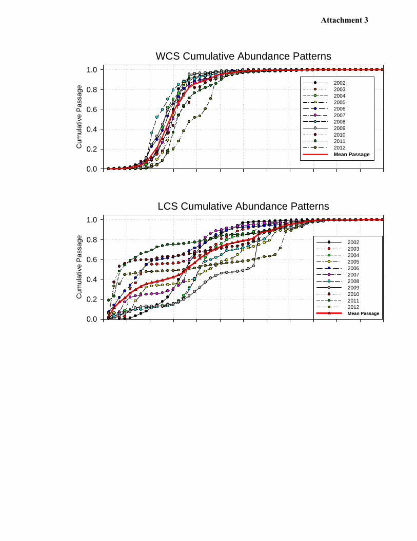
WCS Cumulative Abundance Patterns

Cum

ulat

ive

Pas

sage

0.0

0.2

0.4

0.6

0.8

1.0

20022003200420052006200720082009201020112012Mean Passage

 

 

LCS Cumulative Abundance Patterns

Cum

ulat

ive

Pas

sage

0.0

0.2

0.4

0.6

0.8

1.0

20022003200420052006200720082009201020112012 Mean Passage

 

 

 

 

 

 

 

Attachment 3

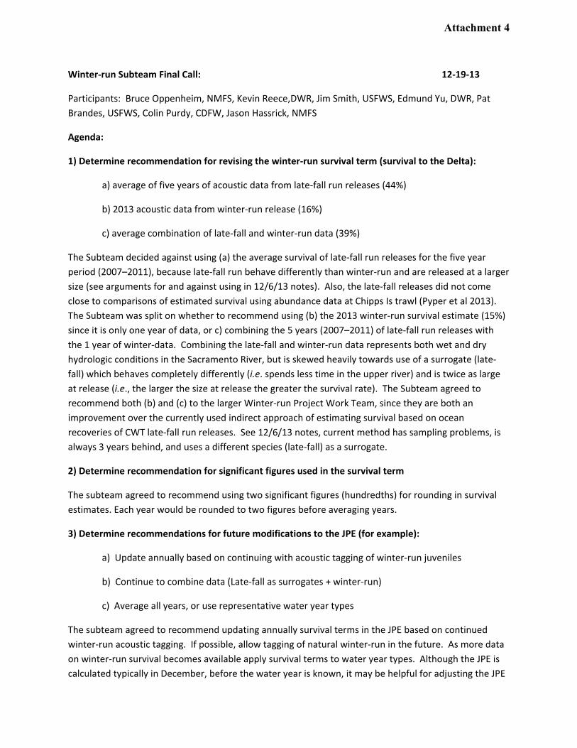
Winter‐run Subteam Final Call:                12‐19‐13 

Participants:  Bruce Oppenheim, NMFS, Kevin Reece,DWR, Jim Smith, USFWS, Edmund Yu, DWR, Pat 

Brandes, USFWS, Colin Purdy, CDFW, Jason Hassrick, NMFS 

Agenda: 

1) Determine recommendation for revising the winter‐run survival term (survival to the Delta): 

a) average of five years of acoustic data from late‐fall run releases (44%) 

b) 2013 acoustic data from winter‐run release (16%) 

c) average combination of late‐fall and winter‐run data (39%) 

The Subteam decided against using (a) the average survival of late‐fall run releases for the five year 

period (2007–2011), because late‐fall run behave differently than winter‐run and are released at a larger 

size (see arguments for and against using in 12/6/13 notes).  Also, the late‐fall releases did not come 

close to comparisons of estimated survival using abundance data at Chipps Is trawl (Pyper et al 2013).  

The Subteam was split on whether to recommend using (b) the 2013 winter‐run survival estimate (15%) 

since it is only one year of data, or c) combining the 5 years (2007–2011) of late‐fall run releases with 

the 1 year of winter‐data.  Combining the late‐fall and winter‐run data represents both wet and dry 

hydrologic conditions in the Sacramento River, but is skewed heavily towards use of a surrogate (late‐

fall) which behaves completely differently (i.e. spends less time in the upper river) and is twice as large 

at release (i.e., the larger the size at release the greater the survival rate).  The Subteam agreed to 

recommend both (b) and (c) to the larger Winter‐run Project Work Team, since they are both an 

improvement over the currently used indirect approach of estimating survival based on ocean 

recoveries of CWT late‐fall run releases.  See 12/6/13 notes, current method has sampling problems, is 

always 3 years behind, and uses a different species (late‐fall) as a surrogate. 

2) Determine recommendation for significant figures used in the survival term 

The subteam agreed to recommend using two significant figures (hundredths) for rounding in survival 

estimates. Each year would be rounded to two figures before averaging years. 

3) Determine recommendations for future modifications to the JPE (for example): 

a)  Update annually based on continuing with acoustic tagging of winter‐run juveniles 

b)  Continue to combine data (Late‐fall as surrogates + winter‐run) 

c)  Average all years, or use representative water year types 

The subteam agreed to recommend updating annually survival terms in the JPE based on continued 

winter‐run acoustic tagging.  If possible, allow tagging of natural winter‐run in the future.  As more data 

on winter‐run survival becomes available apply survival terms to water year types.  Although the JPE is 

calculated typically in December, before the water year is known, it may be helpful for adjusting the JPE 

Attachment 4

later in the year.  Since the most recent acoustic tag data allows survival estimates by reach, the group 

requested that NMFS define the reaches used for entrance into the Delta.  As for the other survival 

terms used in the JPE, the Subteam agreed to keeping the fry‐to‐smolt survival at 59% since there was 

no new data, and increase the egg‐to‐fry survival from 25 to 27% based on the addition of two more 

years of data at Red Bluff (see 12/6/13 notes).  In the future, consideration should be given to whether 

the 3 survival terms used in the JPE overlap and whether the fry‐to‐smolt survival (59%), which is based 

on fall‐run data from the Tehama‐Colusa spawning channel, could be eliminated. 

 

 

 

 

Attachment 4

State of California – Natural Resources Agency EDMUND G. BROWN JR., GovernorDEPARTMENT OF FISH AND WILDLIFE CHARLTON H. BONHAM, Director Fisheries Branch830 "S" StreetSacramento, CA 95811(916) 327-8840www.wildlife.ca.gov

MEMORANDUM

DATE: January 31, 2014

TO: Mr. Bruce Oppenheim, NMFS, Sacramento Office, and Chair of Winter-run Sub Team

FROM: Mr. Michael Lacy and Dr. Russell Bellmer, CDFW, Fisheries Branch, and Chairs of IEP Winter-run Satellite PWT

SUBJECT: Report titled, “Winter-run Sub team Summary” of the Winter-run Sub Team dated January 22, 2014 (Attached)

A Winter-run sub team was formed at the IEP Winter-run Satellite Project Work Team (WRPWT) meeting on 11/20/13 with the purpose of reviewing and revising survival terms used in the NMFS juvenile production estimate (JPE) in light of recent acoustic tag studies. The sub team met three (3) times to review the most recent data/information and current survival terms. After reviewing the current methodology which is based on the difference in survival rates between late-fall run Chinook coded wire tag (CWT) releases at Battle Creek and in the Delta, the sub team found that the current method has many sampling errors and likely over-estimates the number of natural origin winter-run Chinook entering the Delta. The sub team found that the use of acoustic tag data provided greater accuracy, had fewer sampling errors, and provided confidence intervals not available with the current JPE method; therefore it was considered to be the best available science. The use of acoustic data allowed comparisons of in-river reach survival between specific locations, which was not possible before. The sub team compared survival rates using acoustic tag data between Red Bluff Diversion Dam and Sacramento (Tower Bridge).

The sub team presented four (4) recommendations to the WRPWT:

1) Use of the 2013 winter-run acoustic tag survival (16%) in the JPE calculations2) or combine the 5 year average of late-fall run (2007-2011) and 2013 winter-run acoustic data (39%) in the JPE calculations.3) Apply 2 significant figures to survival terms; and4) change egg-to-fry survival from 25% to 27% based on added 2 years of additional data

The WRPWT members reviewed all documents provided by the sub team and it was the consensus of the group that the sub team did an excellent review, sound analysis of available information, and excellent presentation of the pros and cons of the recommendations.

Conserving California’s Wildlife Since 1870

Attachment 5

SUBJECT: Report titled, “Winter-run Sub team Summary” of the Winter-run Sub Team dated January 22, 2014 (Attached)Page 2The WRPWT members agreed that using study fish from the specific population of management importance (i.e., winter-run Chinook salmon), rather than from a surrogate population (late-fall run Chinook salmon) provides direct information on the influence of unique behaviors and life histories of the winter-run population on survival instead of requiring additional inference regarding surrogacy. However, with very limited (one year) acoustic winter-run data, the WRPWT could also not find consensus supporting a recommendation that NMFS shift to this metric this year. None of the alternatives provided by the sub team was clearly best; each present with strengths and weaknesses of different kinds. Although the WRPWT could not come to consensus about the best alternative to use this year, we are very supportive of undertaking the necessary acoustic studies to allow for a future shift in the JPE to the direct measurement of reach specific survival rate using winter-run Chinook. We feel that the best approach for the long-term is to create a time series of direct annual survival estimates representing different water-year, flow, and outmigrant population size to determine the annual survival coefficients for the JPE.

As to the other three (3) recommendations from the sub team, the WRPWT did not reach consensus on the approach for this year.

Attachment 5