justine dattani, phd thesis - spiral: home dattani ... ology into a data-rich field. ... the data...
TRANSCRIPT

Imperial College London
Department of Mathematics
Exact solutions of master equationsfor the analysis of gene transcription models
Justine Dattani
A thesis submitted in partial fulfilment of the requirements for the degree of Doctor of PhilosophyImperial College London, November 2015

Copyright
The copyright of this thesis rests with the author and is made available under a CreativeCommons Attribution Non-Commercial No Derivatives licence. Researchers are free tocopy, distribute or transmit the thesis on the condition that they attribute it, that theydo not use it for commercial purposes and that they do not alter, transform or build uponit. For any reuse or redistribution, researchers must make clear to others the licence termsof this work.
2
Abstract
This thesis is motivated by two associated obstacles we face for the solution and analysis of
master equation models of gene transcription. First, the master equation – a differential-
difference equation that describes the time evolution of the probability distribution of a
discrete Markov process – is difficult to solve and few approaches for solution are known,
particularly for non-stationary systems. Second, we lack a general framework for solving
master equations that promotes explicit comprehension of how extrinsic processes and
variation affect the system, and physical intuition for the solutions and their properties.
We address the second obstacle by deriving the exact solution of the master equa-
tion under general time-dependent assumptions for transcription and degradation rates.
With this analytical solution we obtain the general properties of a broad class of gene
transcription models, within which solutions and properties of specific models may be
placed and understood. Furthermore, there naturally emerges a decoupling of the dis-
crete component of the solution, common to all transcription models of this kind, and the
continuous, model-specific component that describes uncertainty of the parameters and
extrinsic variation. Thus we also address the first obstacle, since to solve a model within
this framework one needs only the probability density for the extrinsic component, which
may be non-stationary. We detail its physical interpretations, and methods to calculate
its probability density.
Specific models are then addressed. In particular we solve for classes of multistate
models, where the gene cycles stochastically between discrete states. We use the insights
gained from these approaches to deduce properties of several other models. Finally, we
introduce a quantitative characterisation of timescales for multistate models, to delineate
“fast” and “slow” switching regimes. We have thus demonstrated the power of the obtained
general solution for analytically predicting gene transcription in non-stationary conditions.
3

Declaration of originality
I hereby declare that the work presented in this thesis is my own, unless otherwise statedand referenced.
Justine Dattani
4

To my parents,
on whose shoulders I am standing.
5

6

Acknowledgments
I am incredibly priviledged and grateful to have had Prof. Mauricio Barahona as my PhDsupervisor; it is difficult to describe the all-permeating effects of his support, guidance,presence, and friendship on my academic development and general well-being, withoutdegenerating into paragraphs of flowery superlatives. He is a true super-human, and Iadmire him more than his modesty would allow him to acknowledge.
I thank the Engineering and Physical Sciences Research Council (EPSRC) and theDepartment of Mathematics at Imperial College London for funding my PhD, and givingme the opportunity to attend numerous conferences and workshops. I would also like tothank Philipp, Ed, Juan, and Andrea who proofread chapters and gave me invaluablefeedback, as well as all the people who worked behind the scenes to provide help andsupport, in particular Dr John Gibbons, Dr Tony Bellotti, Rusudan Svanidze, AndersonSantos, and Kalra Taylor.
The past 4 years would have been comparatively colourless without the friendship andsupport of my office mates over the years, who ensured that no workday was ever dull:Michael, Mariano, Antoine, Elias, Juan, and Ben, I’m going to miss you.
I would especially like to thank Ed for his friendship, love and support, and for keepingme happy, fed, and relatively rested during crunch time. Finally, I would not be here todaywithout my parents Anne-Marie and Satish, who have always done everything they couldso that I could do anything I wanted to. This thesis is their achievement too.
Justine DattaniLondon, February 2016
7

8

Contents
I Introduction to gene transcription models and master equations 17
1 Introduction 191.1 Brief review of approaches for the stochastic modelling of gene transcription 211.2 Outline of the thesis . . . . . . . . . . . . . . . . . . . . . . . . . . . . . . . 23
2 Preliminaries 252.1 Biological background and context . . . . . . . . . . . . . . . . . . . . . . . 25
2.1.1 Gene expression . . . . . . . . . . . . . . . . . . . . . . . . . . . . . 252.1.2 Transcriptional regulation . . . . . . . . . . . . . . . . . . . . . . . . 262.1.3 Experimental capabilities and data . . . . . . . . . . . . . . . . . . . 27
2.2 Master equations for gene transcription . . . . . . . . . . . . . . . . . . . . 302.2.1 Derivation of the master equation . . . . . . . . . . . . . . . . . . . 30
II Exact solution of the master equation 35
3 Derivation of the solution 393.1 Theoretical framework . . . . . . . . . . . . . . . . . . . . . . . . . . . . . . 393.2 The exact Poisson mixture solution . . . . . . . . . . . . . . . . . . . . . . . 413.3 Discussion . . . . . . . . . . . . . . . . . . . . . . . . . . . . . . . . . . . . . 46
4 On the mixture density fXt 494.1 Physical interpretations and intuition . . . . . . . . . . . . . . . . . . . . . . 49
4.1.1 Static cell-to-cell correlations . . . . . . . . . . . . . . . . . . . . . . 494.1.2 Dynamic cell-to-cell correlations . . . . . . . . . . . . . . . . . . . . 514.1.3 Relationship to ODE models of gene transcription . . . . . . . . . . 53
4.2 Obtaining fXt using the differential equation for Xt . . . . . . . . . . . . . 554.2.1 Obtaining fXt via a change of variables . . . . . . . . . . . . . . . . 564.2.2 Reduction of simulation costs . . . . . . . . . . . . . . . . . . . . . . 58
4.3 Kramers-Moyal equation for fXt . . . . . . . . . . . . . . . . . . . . . . . . 594.3.1 The Fokker-Planck equation can only be an approximation . . . . . 61
4.4 Multistate Kramers-Moyal equation . . . . . . . . . . . . . . . . . . . . . . 634.5 Equation for fXt using Fourier transforms . . . . . . . . . . . . . . . . . . . 674.6 Discussion . . . . . . . . . . . . . . . . . . . . . . . . . . . . . . . . . . . . . 69
9

5 Averaging in space or time 715.1 Ensemble moments . . . . . . . . . . . . . . . . . . . . . . . . . . . . . . . . 72
5.1.1 Derivation of the ensemble moments of Nt . . . . . . . . . . . . . . . 735.1.2 Ensemble Fano factor . . . . . . . . . . . . . . . . . . . . . . . . . . 745.1.3 Squared coefficient of variation . . . . . . . . . . . . . . . . . . . . . 76
5.2 Stationarity and ergodicity . . . . . . . . . . . . . . . . . . . . . . . . . . . 775.2.1 Alternative solution for ergodic systems . . . . . . . . . . . . . . . . 815.2.2 Temporal Fano factor . . . . . . . . . . . . . . . . . . . . . . . . . . 86
5.3 Discussion . . . . . . . . . . . . . . . . . . . . . . . . . . . . . . . . . . . . . 87
III Multistate models 89
6 Cyclic models 936.1 Theoretical framework for the M -cycle model . . . . . . . . . . . . . . . . . 936.2 Solution for P (n) via the probability generating function . . . . . . . . . . . 95
6.2.1 Derivation of the solution . . . . . . . . . . . . . . . . . . . . . . . . 956.2.2 Noise regulation . . . . . . . . . . . . . . . . . . . . . . . . . . . . . 101
6.3 Estimating parameter values and model selection . . . . . . . . . . . . . . . 1046.3.1 Generating in-silico data . . . . . . . . . . . . . . . . . . . . . . . . 1056.3.2 Maximum Likelihood estimation and model selection . . . . . . . . . 105
6.4 Solution for fX . . . . . . . . . . . . . . . . . . . . . . . . . . . . . . . . . . 1096.4.1 Derivation of the solution . . . . . . . . . . . . . . . . . . . . . . . . 1096.4.2 Using the mixing density to analyse parameter spaces . . . . . . . . 115
6.5 Final remarks . . . . . . . . . . . . . . . . . . . . . . . . . . . . . . . . . . . 117
7 Which models are solvable? 1217.1 Insights for Markov chain multistate models using Fuchsian theory . . . . . 121
7.1.1 Interlude: A very brief introduction to Fuchsian systems . . . . . . . 1227.1.2 Multistate Kramers-Moyal equations are Fuchsian . . . . . . . . . . 1247.1.3 Two-state model as a Fuchsian system . . . . . . . . . . . . . . . . . 1267.1.4 L-state models with two distinct transcription rates . . . . . . . . . 1297.1.5 Three-state models with three distinct transcription rates . . . . . . 132
7.2 ON-OFF models with non-Markovian promoter switching . . . . . . . . . . 1347.2.1 McFadden interval pdfs . . . . . . . . . . . . . . . . . . . . . . . . . 1357.2.2 Gamma waiting time densities . . . . . . . . . . . . . . . . . . . . . 136
7.3 Discussion . . . . . . . . . . . . . . . . . . . . . . . . . . . . . . . . . . . . . 137
8 Quantification of timescales 1398.1 The mean-first-passage time between stable states . . . . . . . . . . . . . . 1408.2 Derivation of E (Tup) and E (Tdown) . . . . . . . . . . . . . . . . . . . . . . . 1418.3 Regime characterisation using expected waiting times . . . . . . . . . . . . 145
10

8.4 Quantification of parameter regimes from published experiments . . . . . . 1488.5 Final remarks: Effects of waiting time densities . . . . . . . . . . . . . . . . 149
IV Further directions and discussion 151
9 Further directions 1559.1 ON-OFF feedback models . . . . . . . . . . . . . . . . . . . . . . . . . . . . 1559.2 Obtaining equations for fXt . . . . . . . . . . . . . . . . . . . . . . . . . . . 1579.3 First order autoactivation model . . . . . . . . . . . . . . . . . . . . . . . . 1619.4 First order autorepression model . . . . . . . . . . . . . . . . . . . . . . . . 1629.5 Further remarks . . . . . . . . . . . . . . . . . . . . . . . . . . . . . . . . . 163
10 Summary and discussion 165
Summary of permission for third party copyright works 183
11

12

List of Figures
2.1 Time-lapse microscopy using the MS2-GFP detection system . . . . . . . . 272.2 Single-molecule snapshot measurements of mRNA molecules in mouse liver 28
4.1 The effects of synchrony on a toy model with sinusoidal transcription rate . 514.2 Sample paths and probability distributions for a model with temporal con-
trol of the transcription rate . . . . . . . . . . . . . . . . . . . . . . . . . . . 524.3 Approximating fX via stochastic simulations . . . . . . . . . . . . . . . . . 594.4 Sample path of mRNA copy number for a model with Poisson white noise . 68
5.1 Spatial statistics and comparison of simulation results for the Kuramotomodel . . . . . . . . . . . . . . . . . . . . . . . . . . . . . . . . . . . . . . . 76
5.2 Time dependence of the random telegraph model describes only exponentialconvergence to the stationary distribution . . . . . . . . . . . . . . . . . . . 81
5.3 Comparison of models with periodic or stochastic transcription rate over arange of timescales . . . . . . . . . . . . . . . . . . . . . . . . . . . . . . . . 85
5.4 Temporal Fano factor over time for a single sample path of the leaky randomtelegraph model . . . . . . . . . . . . . . . . . . . . . . . . . . . . . . . . . . 87
6.1 M -cycle model of gene transcription . . . . . . . . . . . . . . . . . . . . . . 946.2 Probability mass functions and cumulative mass functions for the NcKap1
MLE results . . . . . . . . . . . . . . . . . . . . . . . . . . . . . . . . . . . . 1076.3 Probability mass functions and cumulative mass functions for the Hmga2
MLE results . . . . . . . . . . . . . . . . . . . . . . . . . . . . . . . . . . . . 1086.4 fX and corresponding P (n) for four qualitatively different behaviours of fX 1166.5 Identification of parameter regimes that give rise to desired qualitative char-
acteristics of the 2-cycle relative to the 1-cycle . . . . . . . . . . . . . . . . 1176.6 OFF-OFF-ON model of gene transcription . . . . . . . . . . . . . . . . . . . 118
7.1 Three-state ladder models of gene transcription . . . . . . . . . . . . . . . . 132
8.1 Characteristic timescales of the switching transients . . . . . . . . . . . . . 1418.2 Classification of parameter regimes in a normalised space that quantita-
tively delineates between “fast” and “slow” switching dynamics . . . . . . . 1478.3 Comparison of parameter regimes implied by fitting the 1-cycle and the
M -cycle to the same data . . . . . . . . . . . . . . . . . . . . . . . . . . . . 149
9.1 ON-OFF feedback models of gene transcription . . . . . . . . . . . . . . . . 158
13

14

List of Tables
6.1 Results of the maximum likelihood estimation procedure for in silico pop-ulation snapshot data . . . . . . . . . . . . . . . . . . . . . . . . . . . . . . 106
15

16

Part I
Introduction to gene transcriptionmodels and master equations
17

18

Chapter 1
Introduction
As early as the 1920s geneticists predicted that genes could “play a fundamental role indetermining the nature of all cell substances, cell structures and cell activities” (Muller1922; Pontecorvo 1968), via a “giant hereditary molecule” (Koltsov (1927), as cited inSoyfer 2001). It is now known that genetic information is transferred to the biologicalsystem via the reproduction (transcription) of a section of DNA (a gene) to producemessenger RNA (mRNA) molecules; the mRNA molecules are then used as templatesfor the synthesis of a protein, or small number of proteins (translation). This process ofinformation transfer is known as gene expression, and occurs in all known life forms tocontrol the structure, functions, decision processes, adaptability, and phenotypes of thecell. Understanding gene expression and its regulation is thus an issue of fundamentalinterest.
Despite gene expression being a control mechanism, its coordination is mired in mys-tery. The process requires a complex sequence of biological steps and potentially involvesa very low number of biomolecules, leading to a distinct kind of heterogeneity at thesingle cell level, beyond the standard randomness and variability widely present in bio-chemical systems. Heterogeneity is observed ubiquitously, even in clonal cell populationsin a homogeneous environment (Elowitz and Leibler 2000; Elowitz et al. 2002; Ozbudaket al. 2002; Blake et al. 2003; Raj et al. 2006; Zenklusen et al. 2008; Zenobi 2013; BaharHalpern et al. 2015), and across time in single cells (Rosenfeld et al. 2005; Golding et al.2005; Cai et al. 2006; Stevense et al. 2010; Yunger et al. 2010; Suter et al. 2011; Harperet al. 2011; Larson et al. 2013; Corrigan and Chubb 2014; Francesconi and Lehner 2014;Singer et al. 2014). So much so, that gene expression is now routinely labelled as beinga “fundamentally stochastic process” (Elowitz et al. 2002; Raser and E. K. O’Shea 2005;Kærn et al. 2005; Raj and Oudenaarden 2008; Raj and Oudenaarden 2009; Shahrezaeiand Swain 2008; Li and Xie 2011; Junker and Oudenaarden 2014). Since expression levelshave such important consequences for the proper functioning of the cell and the cell pop-ulation as a whole, the challenge of understanding gene expression brings us towards therealms of philosophy: how do cells operate with such randomness at their local level, yettogether they form a sentient being that can philosophise about how it can write aboutphilosophising? In that sense, the study of gene expression forms part of the “quantumfield theory” of biology1.
1In fact, Erwin Schrödinger himself addressed these questions in his book What is life? (Schrödinger1948).
19

Part I, Chapter 1 – Introduction
One can argue that, almost by definition, interesting philosophical questions have astheir essence innumerable facets, and are intractably nested in layers of other questions.It is ‘turtles all the way down’, even in a grain of salt2. The questions of life, even froma purely biological viewpoint, are a case in point; a real understanding of gene expressionand its regulation is hindered by the complexity of each cell, each network of intracellularinteractions and molecular species, and how each cell positions itself and its contributionswithin a wider population of cells and their own fluctuating environment, to name but afew of the turtles (Burger 1999; Tanaka et al. 2003; Rockman and Kruglyak 2006; Junkerand Oudenaarden 2014). We are only able to observe relatively few of the factors thatdetermine gene expression and regulation at any one time. The data we obtain can bethought of as the output from a black box, that contains all the information and processesthat we have not observed (Lestas et al. 2010).
The rapid technological advances of this century are transforming molecular cell bi-ology into a data-rich field. Mathematical models and analysis are now essential toolsfor increasing the yield of information from experiments by extracting information fromthe data and inferring properties hidden within the black box. However, the utility ofthe current mathematical models commonly used in the field is reaching two bottlenecks.First, we need to obtain exact, analytical solutions of models that match thekind of data being produced. Since we are now able to capture single-molecule mRNAcounts that change stochastically over time, mathematical formulations and understand-ing must be in terms of discrete probability distributions. We need to solve models thatgive us full, time-dependent distributions of integer random variables, not just averages,continuous approximations or stationary snapshots. Second, in order to keep up with theextraordinary rate at which experiments are performed, we are in particular need ofmathematical models and their properties that are general enough to be appli-cable to a wide range of investigations and datasets, while also being adaptableto each experimental hypothesis.
With these requirements in mind, Part II of this thesis answers the first bottleneck bypresenting the exact solution and properties of a broad class of gene transcription models.The mathematical framework this provides is general enough to include several of the mostwell-used models as specific cases, and naturally accounts for non-stationary systems. Inso doing, we respond to the second bottleneck. In Part III some of the general results areapplied to the commonly-used class of multistate models. The use of a general framework,rather than solving individual models one-by-one, gives us a contextual vantage pointfrom which we can gain physical intuition and predict several fruitful further directions.Exact expressions are also derived for a quantitative characterisation of timescales, andimplications in the context of a broad class of relevant gene transcription models arediscussed. Finally, further directions to explore are discussed in Part IV.
The mathematical framework that will be considered here is not restricted in its scopeto modelling gene transcription; the results are directly applicable to several gene expres-
2See Carl Sagan’s short essay Can we know the universe? Reflections on a grain of salt (Sagan 1979).
20

1.1. Brief review of approaches for the stochastic modelling of gene transcription
sion models for protein levels that use timescale arguments to omit transcription (Paulsson2004; Hornos et al. 2005; Iyer-Biswas et al. 2009; Ge et al. 2015). Further afield, our frame-work it is analogous to G/G/∞ systems in queueing theory (Brémaud 2001; Kendall 1953).We will also draw upon several concepts and classical results from other fields, includingstochastic processes, engineering, and the analysis and geometry of differential equations.However, the motivation to solve models of gene transcription has driven the direction ofthis work, so the focus of the physical interpretations and applications will remain firmlyon mRNA molecules as the objects of interest. A comprehensive account of the fields ofresearch that form the context of this work will not be helpful here, since they are bothvast and advancing at pace. The following brief review sets out the biological backgroundand quantitative paradigms that constitute the motivational basis of this work, focusingon the aspects of stochastic gene expression and master equation models of gene tran-scription that will be most relevant in this thesis. For more general overviews and furtherreading I recommend (Kærn et al. 2005; Raj and Oudenaarden 2008; Li and Xie 2011;Satija and Shalek 2014; Levine et al. 2014) for the causes and consequences of stochasticgene expression and heterogeneity, transcriptional machinery, and experimental strategies,and (Wilkinson 2009; Coulon et al. 2013; Sanchez-Osorio et al. 2014) for some quantitativeapproaches for modelling stochastic gene expression.
1.1 Brief review of approaches for the stochastic modelling of gene transcription
While this thesis has been motivated so far in the context of heterogeneous gene expression,and the increasing volume and quality of experimental data, variation in gene expressionis not itself a new discovery. Indeed, by 1932 Haldane was already predicting differencesin the time of action of genes (Haldane 1932), although it took several decades for clearexperimental evidence to emerge (Schwartz 1962; Spudich and Koshland Jr 1976). Themeasurements of gene products themselves were often limited to protein concentrations,which could be described in detail by traditional rate equations – ODE formulations ofindividual reactions and species (Smolen et al. 2000).
Observed fluctuations were, however, recognised as phenomena worthy of investiga-tion. Differing attitudes for which level to view the fluctuations from led to the emer-gence of two main approaches for modelling the stochasticity. The Langevin approachmaintained the viewpoint of chemical concentrations as the measurements of fundamentalinterest. Drawing upon the central limit theorem, the fluctuations were assumed to beGaussian and theoretical results were based on applications of the fluctuation-dissipationtheorem (Nitzan et al. 1974; Keizer 1975; Keizer 1976; Keizer 1977; Grossmann 1976).The second approach left the perspective of concentrations behind, in favour of the moreelementary viewpoint based on the collision theory of chemical reactions. Believing thatthe state of a chemical reaction system should describe the number of molecules, not theconcentration, stochasticity emerged naturally from the idea that chemical reactions takeplace when diffusing molecules collide with sufficient energy. The resulting differential-
21

Part I, Chapter 1 – Introduction
difference equations for the probability distributions of the number of molecules of eachchemical species of interest became known as the chemical master equations, or simply,master equations (Kramers 1940; Montroll and Shuler 1957; Bartholomay 1958; McQuarrie1967; Gardiner and Chaturvedi 1977; Kampen 1992).
However, the use of stochastic modelling in molecular biology was slow to take hold.This was partly due to a belief that for simple reactions, the probability distributionof the number of molecules in the system exhibits only small fluctuations around themean (McQuarrie 1967), but also because the master equations could only be solved for ahandful of simple reactions (Kampen 1992; Gillespie 1977; Gardiner et al. 1976; Berg 1978).Various methods were developed, including van Kampen’s system size expansion (Kampen1976; Kampen 1992), generating function methods (Bartholomay 1958; McQuarrie 1967),and Gardiner’s Poisson expansion (Gardiner and Chaturvedi 1977), but the methods couldnot always be applied systematically and were not easy to use. In practice, Gillespie’sexact stochastic simulation algorithm (Gillespie 1976; Gillespie 1977) was (and still is)used instead, which does not give expressions for the distributions that can be analysedmathematically.
For studies in gene expression, the lack of reliable single-cell data was an additionalmajor hindrance to motivating the use of master equation models. However, a shift in thatdirection was sparked by the pioneering work of Ko and his co-workers in the early 1990s.They obtained fluorescence intensity data for expression of the β-galactosidase gene insingle cells under different induction doses (Ko et al. 1990). The expression data displayedclear bimodality, meaning that the distributions had clear peaks at two distinct levels ofexpression. Since expression levels were not distributed around the mean value, traditionalODE models would not be able to capture the characteristics of the data. The data alsoconfirmed a conclusion reached several decades before by Novick and Wiener (Novickand Weiner 1957) that induction increased the proportion of cells with high expressionlevels, rather than increasing the expression in each cell linearly. However, Ko went a stepfurther in 1991 by proposing a corresponding stochastic model where in each cell the geneswitches between an active (ON) state, and an inactive (OFF) state according to a time-homogeneous Markov chain (Ko 1991). The implication was that gene expression levelswould change in single cells over time, since trancription would only occur during periodswhen the gene is active. This picture, usually referred to as transcriptional bursting ortranscriptional pulsing, is now known to be a common characteristic of gene expression,from bacteria to mammals (Blake et al. 2003; Raser and E. J. O’Shea 2004; Rosenfeld et al.2005; Golding et al. 2005; Raj et al. 2006; Chubb et al. 2006; Shahrezaei and Swain 2008;Stevense et al. 2010; Larson et al. 2013). Furthermore, since the master equation for Ko’sON-OFF model (also known as the random telegraph model) was solved exactly underthe assumption of ergodicity (Peccoud and Ycart 1995; Raj et al. 2006; Iyer-Biswas et al.2009), it has become widely used to explain the variability observed in gene expressiondata (Raj et al. 2006; Zenklusen et al. 2008; Suter et al. 2011; Larson et al. 2013).
As our experimental capabilities progress, the limitations of the two-state ON-OFF
22

1.2. Outline of the thesis
model and its solution are becoming increasingly evident. First, several studies haveshown that mechanisms for regulating transcription initiation can be highly complex andcombinatorial, and as such they are major sources of gene variability, including nucleosomeoccupancy, TATA box strength, the number of transcription factor binding sites, andtheir location on the promoter (Blake et al. 2006; Sánchez et al. 2008; Sánchez et al.2013; Senecal et al. 2014; Jones et al. 2014; Francesconi and Lehner 2014; Lin et al.2015). Some regulatory factors can induce different transcription rates, or interact witheach other in various ways, so that multi-state extensions of the two-state model areappropriate (Sánchez and Kondev 2008; Coulon et al. 2013; Sánchez et al. 2013; Senecalet al. 2014; Corrigan and Chubb 2014). Second, since the two-state model assumes thatthe gene state switching events are modelled by a Markov chain with constant transitionrates, waiting times in each state are exponentially distributed. However, recent time-lapse recordings of mammalian gene expression show peaked waiting time distributionsin the inactive state (Suter et al. 2011; Harper et al. 2011), suggesting that at least twoinactive states or non-Markovian dynamics at the promoter are necessary to capture theobserved refractory periods. Third, feedback motifs are known to be a common feature ofgene regulatory networks (Shen-Orr et al. 2002; Ji et al. 2013; Kueh et al. 2013), whichare not accounted for in the two-state model. Fourth, the model possesses a stationarysolution, so is unable to describe the observations of time-varying distributions that aredue to, for example, circadian genes (Bieler et al. 2014; Lück et al. 2014; Suter et al.2011), the cell cycle (Spellman et al. 1998; Sigal et al. 2006; Singer et al. 2014), externalsignalling (Larson et al. 2013; Corrigan and Chubb 2014; Olson et al. 2014), or couplingbetween cells (Feillet et al. 2014; Kuramoto 1975).
Unfortunately, exact solutions of the master equation for models of these observationsare rare, and are usually stationary solutions obtained via a probability generating func-tion (Hornos et al. 2005; Zhang et al. 2012; Huang et al. 2014). Instead, quantitativemodelling and analysis of the stochasticity observed in gene expression data must stillbe done via the methods known in the 1970s (McQuarrie 1967; Kampen 1992; Gardiner1985), moment-based measures of noise (Swain et al. 2002; Thattai and Oudenaarden2001), spectral methods (Walczak et al. 2009), approximations of the master equationunder various assumptions including timescale separations (Shahrezaei and Swain 2008;Thomas et al. 2012), numerical solutions (Munsky and Khammash 2006), or stochasticsimulations of the time evolution of the cell population (Gillespie 1976; Gillespie 1977).A general framework for gene transcription models that is applicable to non-stationarysystems is lacking. To fill this gap is precisely the aim of this thesis.
1.2 Outline of the thesis
The following chapter covers some preliminary material on the biological processes anddata that motivate the models we consider, and a simplified derivation of the master equa-tion itself for chemical reactions that are relevant to gene transcription and degradation
23
Part I, Chapter 1 – Introduction
of gene products.Part II gives results within the general framework that we consider, namely models of
mRNA transcription and degradation with time-varying rates and cell-to-cell correlations.Chapter 3 lays down this general theoretical framework, and I show that the solution of themaster equation in this general setting always takes the form of a Poisson mixture distri-bution. The random variable described by the mixing density is completely characterisedby the transcription and degradation rates of the model. In effect, the general solutiondecouples the discrete Poisson contribution of the solution that is common to all genetranscription models, from the model-specific extrinsic component that is encapsulatedentirely in the mixing density. Obtaining the solution of any gene transcription model isthus reduced to the task of calculating the model-specific mixing density; Chapter 4 givessome intuition for the physical interpretation of the extrinsic component, and the advan-tages conferred to us by decomposing the solution in this way. In particular, the extrinsicrandom variable is continuous and naturally encompasses time-dependent correlations be-tween cells, and there are several classical methods for obtaining its probability density.In Chapter 5 the ensemble and temporal moments and measures of noise are discussed asstraightforward corollaries of the full Poisson mixture solution.
Part III focuses on the implications of the general results from Part II on the multistatepromoter models that are found ubiquitously in the analysis of gene expression data.Chapter 6 derives the solution of the cyclic promoter progression model in two differentways, each giving us different tools for analysis and understanding of the behaviour of thesolution. Chapter 7 capitalises on the extra structural knowledge of model solutions thatwe obtain by determining the mixing density to infer which other models can be solvedand the forms of their solutions. In Chapter 8 an exact quantitative characterisation of thetimescales implied by ON-OFF model parameters is derived, and the validity of timescaleseparation arguments is discussed in terms of recent time-lapse experimental data fromthe literature.
Finally, Chapter 9 in Part IV discusses the connections of our framework to Pois-son expansions of feedback models, the potential gains from extending the framework tofeedback models, and proposes some initial approaches for pursuing them.
24

Chapter 2
Preliminaries
The purpose of this chapter is to provide only the necessary background material and andcontext for what follows in the rest of the thesis. We first give a basic introduction to theprocesses involved in gene expression and transcriptional regulation, based on Alberts etal. 2008, followed by an overview of the types of data that motivate our theoretical work.The following section gives a short derivation of the master equation for the single-speciesmodels that we will consider.
2.1 Biological background and context
2.1.1 Gene expression
Biology is a science of incredible diversity, based upon a set of common underlying princi-ples. From the relatively simple, single-celled archaea to large, highly complex organisms,common to all life forms1 is the cell as the fundamental unit of life. At the cellular leveltoo, there can be hundreds of different cell types that form a single species, yet the under-lying principles of structure and function share a number of common traits. In particular,for both prokaryotes (single-celled organisms without a nucleus, i.e. archaea and bacteria)and eukaryotes (organisms whose cells have a nucleus) the mechanisms for storing andusing hereditary information that influences form and function of all organisms are sur-prisingly similar; the information is stored in coded form as a sequence using four letters,within the now famous deoxyribonucleic acid (DNA) molecules.
In the traditional view, the information is divided into units, called genes, each of whichencodes a defined protein component. However, several more recent findings require theconcept of a gene to be revised. For example, alternative splicing allows a single sectionof DNA to code for multiple proteins, and some genes code for functional products thatare not used to synthesize proteins. Since there is no widely accepted consensus on thedefinition of a gene, for the modelling in this thesis it will be adequate to think of it as aparticular locus of a DNA molecule, that is copied to make the products we are interestedin.
Although DNA encodes all the necessary information to replicate an organism, theinformation needs to be expressed in order to produce the gene products that are requiredby the cell. Different cells need different gene products in varying amounts, at differenttimes, and according to its environment, so the cell expresses the information from the
1The classification of viruses as non-cellular life forms is still a controversial issue (Forterre 2010).
25

Part I, Chapter 2 – Preliminaries
relevant genes when required, in a process known as gene expression. There are severalsteps involved, but gene expression can be broadly split into two processes: transcription,followed by translation.
In transcription, the gene is copied, or transcribed, into a ribonucleic acid (RNA)molecule. The resulting RNA molecule is therefore sometimes referred to as a transcript.Since the gene can be used repeatedly for transcription, the transcript is a disposablecopy of the information stored in the DNA. The RNA molecules that serve as messengersof this information to guide protein synthesis are known as messenger RNA (mRNA)molecules, and are the type that we model in this thesis. Molecular complexes calledribosomes translate the mRNA molecules into proteins, in a process known as translation.Depending on its stability, each mRNA molecule can be used to synthesize many proteinmolecules before being degraded.
We will be concerned with modelling transcription. Since translation does not expendmRNA molecules, in general we will not need to consider translation in a direct manner.
2.1.2 Transcriptional regulation
Every cell needs to be able to control the type and amount of proteins and other geneproducts, in order to interact with and respond to internal signals, to other cells, and totheir environment in general. In a multicellular organism, each DNA molecule has thesame sequence and therefore the cell type depends on which genes are expressed, andwhich aren’t. Regulation of gene expression is thus essential for the proper and efficientfunctioning of any cell.
The main control point for gene regulation is at the start of the gene expression process,where the gene can be turned ‘on’ or ‘off’ (see Fig. 2.1 E,F). The strategies and mechanismsused for activating or inhibiting transcription initiation are numerous, and are generallydifferent for prokaryotic and eukaryotic cells. To limit our scope, we will focus on thegeneral mechanisms that motivate our work and are necessary to understand it.
For both prokaryotes and eukaryotes, transcription is initiated when an RNA poly-merase molecule binds to the promoter, a specialised sequence on the DNA strand that isusually located just upstream of the starting point for transcription. Regulatory proteinscalled transcription factors (TFs) bind to the DNA at specific loci in order to influence theaction of the RNA polymerase. In bacteria, genes are ‘on’ by default, so repressor proteinsare their main tools for the regulation of gene expression (Jacob and Monod 1961). Therepressor binds to the DNA close to the promoter site, thus blocking the RNA polymerasefrom binding and initiating transcription. When the repressor unbinds from its positionon the DNA strand, for example due to a conformational change caused by the binding ofanother regulatory molecule, the gene is available for transcription once more (Jacob andMonod 1962).
Transcriptional regulation is a far more complex process in eukaryotic cells, being acombination of the structural effects of the DNA, and more sophisticated interactions ofTFs. For eukaryotes, TFs usually activate transcription, and their action is said to be
26

2.1. Biological background and context
‘combinatorial’ (Remenyi et al. 2004; Lin et al. 2015): regulation requires interactionsbetween several proteins; RNA polymerase is often not able to bind to the promoter with-out this recruitment by TFs (Struhl 1999). Thus, eukaryotic genes are generally ‘off’ bydefault. The recruitment of TFs can be influenced by several factors, including the ex-istence of a conserved gene sequence called a TATA box, silencer elements for repressormolecules, and chromatin structure. Chromatin is the complex formed by the DNA withproteins, which causes the DNA strands to be highly condensed and wrapped around pro-teins called histones. For TFs to bind to the DNA at the correct positions, the chromatinstructure must be unwound into an ‘open’ domain. Thus even in the presence of severaltranscription factors, the genes in a closed chromatin domain remain inactive.
Figure 2.1: Time-lapse microscopy using the MS2-GFP detection system. (A-D) Fluo-rescence microscopy images of human U2-OS cells at different time points. Transcriptionsites are visible as fluorescent spots. Scale bar = 4 µm. (E, F) Fluorescence of single cellsas a function of time with highlighted ON and OFF intervals of transcription. Reprintedfrom eLife, 2, Larson et al., Direct observation of frequency modulated transcription insingle cells using light activation, e100750 (2013) under the Creative Commons CC0 publicdomain dedication.
2.1.3 Experimental capabilities and dataTo help understand gene expression and its regulation, we would ideally like to observeall the relevant molecules and their interactions, in single cells over time. We are still farfrom this ideal scenario which, given the complexities of gene regulation, may well alwaysremain science fiction. Nevertheless, our experimental capabilities are advancing at anastonishing rate, especially at the mRNA level. Where only a little over a decade ago
27

Part I, Chapter 2 – Preliminaries
single-cell observations of mRNA molecules in living cells were unheard of, we are nowable to reliably observe and quantify single molecules in single cells over time.
With this pace of progress in mind, the gene transcription models considered in thisthesis are formulated mathematically in order to obtain probability distributions for themRNA copy number in single cells over time. Since the main motivation of these modelsis to have the quantitative tools necessary to analyse the single-molecule, time-lapse datathat are emerging, we mention here the main single-mRNA detection approaches thatform the context for the examples we use in the main body of the text.
Population snapshot methods
Figure 2.2: Single-molecule population snapshot measurements of mRNA molecules inmouse liver cells, obtained using smFISH. Top: Red dots are single mRNA molecules,blue areas are stained nuclei, and green is staining of the cell membrane. PP, periportalzone. PC, pericentral zone. Scale bar is 30 mm. Below left: Dual-colour labelling oftranscription sites reveal active transcription sites, indicated by the arrowhead. Belowright: Distribution of the number of mRNA molecules per cell (bars), and theoreticalprobability density functions (lines) from two different mathematical models. Reprintedfrom Molecular Cell, 58, K. Bahar Halpern et al., Bursty gene expression in the intactmammalian liver, 147-156, Copyright 2015, with permission from Elsevier.
Population snapshot approaches tell us the number (or relative number) of mRNAmolecules in single cells of a population, at a single time point. The data is usually
28

2.1. Biological background and context
represented in the form of bar graphs or histograms (see Fig. 2.2 for an example).Single-molecule fluorescence in situ hybridization (smFISH) allows one to count mRNA
molecules in single cells and view their localisation (Femino et al. 1998; Raj and Oude-naarden 2008; Little et al. 2013; Lyubimova et al. 2013). Samples are fixed and thenhybridised using a set of fluorescently labelled oligonucleotides. Although this methodprovides only a single-time picture of the expression levels, the resolution of the moleculesis unparalleled, even with dual-colour labelling (Bahar Halpern et al. 2015).
Single-cell quantitative reverse transcriptase polymerase chain reaction (RT-PCR), anddigital single-cell RT-PCR are highly sensitive methods for counting mRNA molecules inhundreds of single cells. The method yields absolute numbers, rather than arbitraryfluorescence units, but does not give us any spatial information (Bengtsson et al. 2005;Warren et al. 2006; Ståhlberg et al. 2012).
Time-lapse methods
Time-lapse methods rely on engineering cells so that the transcripts of interest fluoresce,usually using fluorescent ‘tagging’ proteins. Previously, resolution at the mRNA level waslow, so we would infer the number of molecules present in a single cell by the fluorescenceintensity. However, methods have improved drastically in the past few years, so we arenow able to track single molecules (Fig 2.1 A-D), as well as obtain time-lapse traces thatindicate the expression levels of single cells over time (Fig 2.1 E-F, for example). As such,we are starting to overcome some of the usual limitations associated with fluorescencemeasurements, i.e., background fluorescence, low resolution, and inferring molecule num-bers from arbitrary fluorescence units. However, the confounding effects of the fluorescenttags must still be kept in mind.
The MS2-GFP mRNA detection system is the predominant procedure for the directobservation of single mRNA molecules in living cells, over time (Bertrand et al. 1998;Golding and Cox 2004; Golding et al. 2005; Muramoto et al. 2012; Larson et al. 2013;Coulon et al. 2014; Corrigan and Chubb 2014). The gene is engineered to encode for anumber of RNA hairpins, and an MS2-coat protein is tagged with a fluorescent protein,usually GFP, that binds with high affinity to the RNA loops (Bertrand et al. 1998; Goldingand Cox 2004). When the MS2-GFP fusion binds to the mRNA, the molecules fluoresceand can be followed over time using time-lapse microscopy (see Fig. 2.1). Two-coloursingle-mRNA imaging is also emerging (Coulon et al. 2014). The main disadvantagefor this method is that degradation of the reporter molecules is strongly inhibited, theexperiments are constrained to timescales of only a few hours, and relatively few cells canbe imaged (Golding et al. 2005).
High-throughput single-molecule assays have been developed recently, although themethod has so far been constrained to in vitro studies (Chong et al. 2014). The methodallows us to monitor the process of transcription itself, so that we can view transcriptioninitiation time points, and measure how long it takes to produce each transcript. A finalapproach worth mentioning, pioneered by the Naef lab, is to measure the fluorescence
29

Part I, Chapter 2 – Preliminaries
of short-lived proteins (Suter et al. 2011; Molina et al. 2013). The protein dynamicsmimic those of the mRNA molecules because of the short half-lives. The cells can then betracked over days instead of hours, and the data is not skewed by the slow degradation ofthe reporter molecules.
2.2 Master equations for gene transcription
In Chapter 1 we laid down the motivations for modelling gene expression with masterequations, and developing a framework for solving them. The purpose of this sectionis to outline the arguments used to derive the master equation, and to acknowledge theunderlying assumptions that are made, so that in later chapters we can start from this basisand immediately write down the master equation for a given model of gene transcription.
2.2.1 Derivation of the master equation
We are interested in modelling Nt, the number of mRNA molecules in a single cell overtime. It is understood that Nt refers only to mRNA molecules that were transcribed at aspecific gene that we are interested in. Since the number of transcripts of any particularkind in a single cell can be very low2, we do not permit Nt to be approximated by acontinuous variable. In other words, Nt takes only non-negative integer values.
As mentioned in Chapter 1, and illustrated by the experimental data in Figs 2.1 and 2.2,Nt changes stochastically in time. To accommodate our discrete, stochastic state variableNt mathematically, we need to describe its value by P (n, t) ..= Pr(Nt = n), the probabilitythat Nt has the value n ∈ N at time t.
Starting from the collision theory of chemical kinetics, that chemical reactions occurwhen two molecules collide with sufficient energy, we can derive an equation for the timeevolution of P (n, t) in a well-stirred system at thermal equilibrium (Gillespie 1992a).Equations of this kind are known generally as Kolmogorov forward equations, but whenthe random variable is discrete, as we have here, they are more often known as chemicalmaster equations, or simply master equations.
It is now known that the cell is a densely crowded, compartmentalised system, so thatmolecules can not freely diffuse within it. Nevertheless, the master equation as derivedusing arguments based on conventional chemical reaction rates has proved incredibly usefulfor characterising and explaining stochasticity in gene expression (McQuarrie 1967). Withthis caveat in mind, we briefly outline these arguments to derive master equations formodels of transcription for a single gene. Extensions for systems with more than onechemical species follow in a similar manner; see any of the references Gardiner 1985;Kampen 1992; Gillespie 1992b for derivations with more generality.
Let o(dt) denote terms such that limdt→0 o(dt)/dt = 0, and let n→ m denote the eventof a transition from state n to state m. We make the following assumptions:
2Average mRNA copy numbers usually range from less than one to a few hundred (Milo and Phillips2015); the median in mammalian cells has been reported as being only 17 (Schwanhäusser et al. 2011).
30

2.2. Master equations for gene transcription
i. The probability of a transition n→ n+ 1 in the infinitesimal time interval (t, t+ dt)is a(n, t)dt+ o(dt), where a(n, t) ∈ R≥0.
ii. The probability of a transition n→ n− 1 in the infinitesimal time interval (t, t+ dt)is b(n, t)dt+ o(dt), where b(n, t) ∈ R≥0.
iii. The probability of a transition n → n ± j, j > 1, in the time interval (t, t + dt) iso(dt).
Notice that under these assumptions, the system has the Markov property: the transitionprobabilities depend only on the current state of the system.
Now P (n, t+ dt) is given by the sum of:
i. the probability that the system is in state n at time t, and remains there until t+ dt,
ii. the probability that the system is in state n− 1 at time t, and transitions to state nby t+ dt
iii. the probability that the system is in state n+ 1 at time t, and transitions to state nby t+ dt, and
iv. the probability that the system is in state n ± j, j > 1 at time t, and transitions tostate n by t+ dt.
Using the multiplication law of probability, i.e. Pr(A and B) = Pr(A) × Pr(B given A),we have
P (n, t+ dt) = P (n, t)× [1− Prn→ n± j, j ≥ 1, in (t, t+ dt)]
+ Prn− 1→ n in (t, t+ dt)
+ Prn+ 1→ n in (t, t+ dt)
+ Prn± j → n, j ≥ 1, in (t, t+ dt)
= P (n, t)[1− a(n, t)dt− b(n, t)dt− o(dt)]
+ P (n− 1, t)[a(n, t)dt+ o(dt)]
+ P (n+ 1, t)[b(n, t)dt+ o(dt)] + o(dt).
Moving the P (n, t) term from the right hand side of the equation to the left, dividing bydt, and taking the limit dt→ 0, we obtain the master equation
dP (n, t)dt
= −[a(n, t) + b(n, t)]P (n, t) + a(n− 1, t)P (n− 1, t) + b(n+ 1, t)P (n+ 1, t).
Suppose the state transition n → n + 1 can only happen via a transcription event, andthe state transition n → n − 1 can only happen via a degradation event. Suppose alsothat mRNA molecules do not directly influence the processes of transcription at theirgene, and degradation. Then transcription is a zero-order chemical reaction: we have
31

Part I, Chapter 2 – Preliminaries
a(n, t) = α(t). On the other hand, degradation is a first-order chemical reaction: for eachmRNA molecule, the probability that it degrades in (t, t+dt) is β(t)dt+o(dt), β(t) ∈ R≥0,so with n mRNA molecules present in a system, the probability of a transition n→ n− 1in (t, t+ dt) is β(t)ndt+ o(dt), i.e. b(n, t) = β(t)n. We are then left with
dP (n, t)dt
= −[α(t) + β(t)n]P (n, t) + α(t)P (n− 1, t) + β(t)(n+ 1)P (n+ 1, t).
Example 2.2–1 walks through the steps of solving a simple master equation model ofgene transcription, using the probability generating function method that we will use inthe next chapter.
Example 2.2–1 — Gene transcription model with constant rates
The most simple gene transcription model assumes a constant transcription rate andlinear degradation, i.e. a(n, t) = α and b(n, t) = βn, where α, β > 0 are constants.The master equation for this model is therefore
dP (n, t)dt
= −[α+ βn]P (n, t) + αP (n− 1, t) + β(n+ 1)P (n+ 1, t). (2.1)
The usual approach for obtaining P (n, t) is to use the probability generating function,namely,
G(z, t) ..=∞∑n=0
znP (n, t),
to transform the master equation (2.1) into a partial differential equation (Bartholomay1958; Kampen 1992; Gardiner 1985). It is fairly straightforward to check that:
∑znP (n, t)dt
= ∂G
∂t∑nznP (n, t) = z
∑ ∂
∂zznP (n, t) = z
∂G
∂z∑znP (n− 1, t) = z
∑zn−1P (n− 1, t) = zG
∑(n+ 1)znP (n+ 1, t) = ∂G
∂z.
so if we multiply Eq. (2.1) through by zn and sum over all n, we can use the identitiesabove to find that G satisfies
∂G
∂t= α(z − 1)G− β(z − 1)∂G
∂z.
We can solve this equation for G using the method of characteristics with initial con-
32

2.2. Master equations for gene transcription
dition P (0, 0) = 1, P (n, 0) = 0 for n > 0, to find
G(z, t) = eαβ
[1−e−βt](z−1). (2.2)
Recall that, by definition, P (n, t) is the coefficient of zn in G(z, t) so by expandingEq. (2.2) we obtain
P (n, t) = 1n!
(α
β
[1− e−βt
])neαβ
[1−e−βt],
i.e.Nt ∼ Poi
(α
β
[1− e−βt
]).
33

Part I, Chapter 2 – Preliminaries
34

Part II
Exact solution of the masterequation
35

36

Part II: Exact solution of the master equation
Introduction
Fundamentally speaking, expression of a single gene can be measured in terms of thenumber of mRNA molecules present that were transcribed at the gene in question. SincemRNA copy number increases only via transcription events and decreases via degradationevents, in a coarse-grained sense gene transcription models simply describe the processesof transcription and degradation. Specificity and complexity of any particular model aredefined by the assumptions and levels of detail used to describe those processes for thecontext in which the model will be used.
In this part we work within the following simple framework: we consider the processesof transcription and degradation in a very general sense, and infer the resulting probabilitydistribution of the mRNA copy number over time, with several corollaries. The constraintson the mathematical or statistical descriptions of transcription and degradation are weak,so the results are applicable to most types of transcription models considered in the field.In particular, time-dependence due to correlated expression between cells in the populationcan be naturally accounted for here, a property that is often lacking in gene transcriptionmodels as stationarity is so often assumed. The chapters in Part III will apply the generalresults given here to more specific descriptions of transcription and degradation.
In Chapter 3, we describe the theoretical framework and derive the main result thatwill underpin the rest of the thesis: that the probability mass function of the mRNA copynumber is always a Poisson mixture. In Chapter 4 we give some physical intuition for themixture distribution, place it into the context of existing approaches for solving models ofgene transcription, and collect together results from several dissociated fields that can helpobtain it. Chapter 5 contains corollaries of the result in Chapter 3 to do with momentsand measures of noise.
37

Part II,
38

Chapter 3
Derivation of the solution
This chapter consists of the foundations that will underpin the rest of this work. Wedescribe the general, theoretical framework and model, and derive the main result that willbe used throughout the thesis. Despite its central importance, the mathematics requiredhere are fairly basic elements of probability theory and stochastic processes. However,it is the tool that has allowed us to understand what is already known about most genetranscription models, as specific cases of this result. This understanding has also guidedus towards all the new results that will be discussed in the rest of the thesis, as it allowsus to decouple the “Poisson” contribution that is common to all gene transcription modelsof the kind we consider, from the model-specific contribution.
3.1 Theoretical framework
We are interested in the expression in time of a specific gene, measured by the number ofmRNA molecules present in each cell of a population that were transcribed at that gene.We assume that the mRNA copy number changes only via transcription and degradationevents, both of which occur according to the principles of stochastic chemical kineticsdescribed in Chapter 2. We will refer to models of this broad category as transcription-degradation models.
Our measure for gene expression, the mRNA copy number, is a stochastic process incontinuous time t which we will denote by
N ≡ Ntt≥0 ≡ t 7→ ηω(t) : ω ∈ ΩN .
Ntt≥0 is a set of random variables Nt, one for each time t, and t 7→ ηω(t) : ω ∈ ΩN isthe set of all possible sample paths for the mRNA copy number in a single cell. We willdenote the probability mass function for Nt by
P (n, t) ≡ Pr(Nt = n), n ∈ N.
If N is a stationary process so that the law of Nt is independent of t, we will simply writeP (n) ≡ Pr(Nt = n).
In order to account for the variability in the transcription and degradation reactionrates, both in time and between cells, we allow them to be described by the stochastic
39

Part II, Chapter 3 – Derivation of the solution
processes
M≡ Mtt≥0 ≡ t 7→ µω(t) : ω ∈ ΩM and
L ≡ Ltt≥0 ≡ t 7→ λω(t) : ω ∈ ΩL ,
respectively. The notation here is the same as that for N : Mt and Lt are random variables,t 7→ µω(t) and t 7→ λω(t) are sample paths of the transcription and degradation rates,respectively, and ΩM and ΩL are the sample spaces. For continuous random variablessuch as Mt and Lt, we will denote the cumulative density function (cdf) and probabilitydensity function (pdf) according to usual conventions with a capital F and lower-case f ,respectively. For example FMt(m, t) and fMt(m, t) are the cdf and pdf of Mt at time t.We will sometimes refer to the transcription and degradation rates collectively as cellulardrives, or simply drives.
We do not specify any functional form for the cellular drives here, except to require thatt 7→ µω(t) and t 7→ λω(t) do not depend on the number of mRNAmolecules already present.Thus these sample paths may be thought of as example functions of time that describethe transcription and degradation rates in response to changing cellular architecture andenvironmental conditions in an example cell. Note that by allowing the drives to bedescribed by stochastic processes in this way, we have the freedom to explicitly specifyhow correlated we would like them to be1. In general, we will mention correlation betweensample paths in a broad manner, rather than in precise, quantitative terms. Therefore, toavoid confusion with statistical measures of correlation and dependence, we will refer tocells or cellular drives as having a “degree of synchrony”. A population will be perfectlysynchronous if the sample paths of the drives for every cell in the population is identical,or equivalently, if Mt and Lt have zero variance. For example, if the transcription rateis a deterministic sinusoidal function t 7→ g(t) and is perfectly synchronous for all cells,we would have fMt(m, t) = δ(g(t) −m) ∀ t ≥ 0, where δ is the Dirac delta function. If,however, cellular variability means that the transcription rate will be slightly out of phasebetween cells, we can impose that fMt be a more dispersed density: the wider the density,the more asynchronous the drive is. This control is discussed in Chapter 4 with severalexamples.
Note also that this framework generalises models that account for each step of tran-scription or degradation individually: the only gene expression model without a time-dependent drive is the standard first-order model with constant transcription and degra-dation rates µ and λ, and stationary solution Nt ∼ Poi(µ/λ)∀ t (see Example 3.2–1). Allother models implicitly or explicitly have drives that are not constant.
Ultimately, we would like to obtain the probability distribution of Nt for all t, withinthis context of time-varying and/or stochastic parameters. The following section derivesan expression for P (n, t) in the general case, which will be used in Chapters 4 and 5 to
1In fact, by defining M and L by the random variables Mt and Lt for each t, we can specify anystatistical characteristics of the population that we choose.
40

3.2. The exact Poisson mixture solution
derive properties of transcription-degradation models, and then throughout the rest of thethesis to solve and analyse several specific gene transcription models.
3.2 The exact Poisson mixture solution
We first consider a population whose cellular drives are perfectly synchronous, and usethe information we gain to derive the probability distribution P (n, t) for the general case.
Perfectly synchronous case: no cell-to-cell variation in cellular drives
Consider first a population of cells with perfectly synchronous transcription and degrada-tion rate functions Msync = µ(t)t≥0 and Lsync = λ(t)t≥0. In other words, every cellin the population has transcription rate t 7→ µ(t) and degradation rate t 7→ λ(t), so Mt
and Lt have zero variance ∀ t ≥ 0. We thus have an immigration-death process that canbe summarized by the following reaction diagram:
∅ µ(t)−−→ mRNA λ(t)−−→ ∅. (3.1)
Note that this is not a birth-death process because the mRNA do not reproduce; so thetranscription rate µ(t) has units t−1. In contrast, degradation is a first-order reaction, sothe unit for the degradation rate is t−1n−1.
Denote the probability mass function for the mRNA copy number Nt for this specialcase with synchronous drives by
Psync(n, t) ..= Pr (Nt = n|Msync,Lsync) .
The master equation for Psync(n, t) is then given by:
d
dtPsync(n, t) = µ(t)Psync(n− 1, t) + (n+ 1)λ(t)Psync(n+ 1, t)
− [µ(t) + nλ(t)]Psync(n, t). (3.2)
Using the definition of the probability generating function
G(z, t) ..=∞∑n=0
znPsync(n, t),
we can transform the master equation (3.2) into
∂G
∂t= (z − 1)µ(t)G− (z − 1)λ(t)∂G
∂z. (3.3)
We will solve this equation using the method of characteristics, assuming for now thatthere are initially n0 mRNA molecules in each cell. Introduce the characteristic equations
dt
ds= 1, dz
ds= (z − 1)λ(t), dG
ds= (z − 1)µ(t)G,
41

Part II, Chapter 3 – Derivation of the solution
where s is a parametrisation of the characteristic curve, and without loss of generality wecan let t(0) = 0. Solving this system, we have
t = s,
z − 1 = [z(0)− 1] e∫ s
0 λ(σ) dσ , and
G(s) = G(0) e[z(0)−1]∫ s
0 µ(τ)e∫ τ
0λ(σ) dσ
dτ .
Noticing that the initial condition P (n0, 0) = 1 implies that G(0) = G(z(0), t(0)) = z(0)n0 ,and eliminating the parameter s, we obtain the solution:
G(z, t|n0) =[(z − 1)e−
∫ t0 λ(τ) dτ + 1
]n0
ex(t)(z−1) (3.4)
=.. GN ict
(z, t)GNst(z, t),
wherex(t) ..=
∫ t
0µ(τ)e−
∫ tτλ(τ ′) dτ ′ dτ. (3.5)
We will refer to x as the extrinsic parameter.
Notice that G(z, t|n0) (Eq. (3.4)) is the product of two probability generating functions:GN ic
t(z, t) is the probability generating function for a binomial random variable N ic
t , with
n0 trials and success probability e−∫ t
0 λ(τ) dτ , and GNst(z, t) is the probability generating
function for a Poisson random variable N st , with parameter x(t). So for this special case
where all cells have perfectly synchronous drives, we deduce (Feller 1968) that
Nt = N ict +N s
t ; (3.6)
N ict ∼ Bin
(n0, e
−∫ t
0 λ(τ)dτ), (3.7)
N st ∼ Poi (x(t)) . (3.8)
The physical interpretation of this breakdown is that N ict describes the mRNA transcripts
that were initially present in the cell and still remain at time t, and N st describes the
number present in the cell that were transcribed since t = 0.
N ict and N s
t are independent, so it is easy to read off the first two moments:
E (Nt|Msync,Lsync, n0) = E(N ict
)+ E (N s
t )
= n0 e−∫ t
0 λ(τ)dτ + x(t),
Var(Nt|Msync,Lsync, n0) = Var(N ict ) + Var(N s
t )
= n0e−∫ t
0 λ(τ) dτ(
1− e−∫ t
0 λ(τ) dτ)
+ x(t).
We can go further and write down the explicit expression for Psync(n, t|n0), either by
42

3.2. The exact Poisson mixture solution
computing the coefficient of zn in G(z, t), or by using Eqs (3.6)-(3.8) to write
Psync(n, t|n0) = Pr(N ict +N s
t = n|n0)
=n∑k=0
Pr(N ict = k|n0) Pr(N s
t = n− k)
=n∑k=0
(n0k
)e−k
∫ t0 λ(τ)dτ
(1− e−
∫ t0 λ(τ)dτ
)n0−k x(t)n−k(n− k)! e
−x(t) .
If the initial condition n0 is not known, or if the state of each cell at t = 0 is not identical,it can be more appropriate to let the initial state be described by a random variable N0.In this case, the law of total probability gives us
Psync(n, t) =∑n0
Psync(n, t|n0) Pr(N0 = n0) . (3.9)
Notice that the contribution from N ict decreases exponentially for any sensible degra-
dation functions λ, as the transcripts that were present at t = 0 are expected to degrade,and the population is expected to be composed only of mRNA molecules that were tran-scribed since t = 0. Hence in this case where all cells are initialised in the same state,the distribution Psync(n, t|n0) displays a transient period until the contribution from N ic
t
is negligible. However, Nt = N ict + N s
t does not necessarily display transient behaviouruntil the contribution from N ic
t is negligible. Let us first fix ideas using a model with astationary solution, and then discuss the general case.
Example 3.2–1 — Time-dependent contributions from N ict and N s
t can bal-ance each other
Consider the gene transcription model with constant transcription and degradationrates µ and λ. Then, when there are initially n0 mRNA transcripts, Eqs (3.6)-(3.8)give us
N ict ∼ Bin
(n0, e
−λt),
N st ∼ Poi
(µ
λ
[1− e−λt
]).
As t→∞ the distribution ofNt will tend towards Poi(µ/λ), the stationary distributionof the population. We will show that if the system starts at stationarity, Nt = N ic
t +N st
will be independent of time ∀ t ≥ 0.
43

Part II, Chapter 3 – Derivation of the solution
Suppose that the population starts at stationarity, i.e.
Pr(N0 = n0) =(µ
λ
)n0 e−µ/λ
n0! .
We wish to find Psync(n, t) given this initial distribution. We still have
N st ∼ Poi
(µ
λ
[1− e−λt
]),
so we just need to determine the contribution to Nt from N ict . In this case, we have
Pr(N ict = k) =
∞∑n0=k
Pr(N ict = k|N0 = n0) Pr(N0 = n0)
=∞∑
n0=k
(n0k
)(e−λt
)k (1− e−λt
)n0−k(µ
λ
)n0 e−µ/λ
n0!
=(e−λt
)ke−µ/λ
∞∑r=0
(µ
λ
)r+k (1− e−λt)r
k! r!
=(µ
λ
)k (e−λt)k e−µ/λk!
∞∑r=0
(µ
λ
)r (1− e−λt)r
r!
=(µ
λe−λt
)k e−µ/λk! e
µλ
(1−e−λt)
=(µ
λe−λt
)k e−µλ e−λtk! .
In other words N ict ∼ Poi
(µλ e−λt), which cancels the time dependent contribution
from N st ∼ Poi
(µλ
[1− e−λt
]). Therefore ∀ t ≥ 0,
Nt ∼ Poi(µ
λ
).
The example shows that N ict and N s
t will combine to reproduce a stationary distributionat all times t > 0, when the system starts at stationarity. Thus we do not have a transientperiod where the initial distribution converges to the equilibrium of the system.
The same is true if the system is not stationary: suppose we let the system start att = −∞, with any initial condition. For t > 0, the system will be independent of the initialcondition and will be described by N s
t . Let us denote the state of the system for t > 0 bythe attracting distribution P∗. Although Pr(N s
t = n) = P∗(n, t) ∀ n ∈ N, ∀ t > 0, we wishto distinguish P∗ from Ps because we only have equality of the two distributions when the
44

3.2. The exact Poisson mixture solution
system starts at t = −∞. P∗ can be thought of as an inherent property of the system,analogous to the the stable point of a dynamical system that moves in time (sometimescalled a chronotaxic system (Suprunenko et al. 2013)).
Now, if we let Pr(N0 = n0) = P∗(n0, 0) ∀ n0 in Eq. (3.9), the contributions fromN ict and N s
t balance each other as they did in Example 3.2–1, and we have Psync(n, t) =P∗(n, t) ∀ n, ∀ t > 0. Thus we only observe an initial transient period if the initialdistribution starts away from its attracting distribution at t = 0. In all other cases,the following mathematical formulations are equivalent: i) assume that the system wasinitialised at t = −∞ and consider only N s
t , or ii) use the initial distribution P∗(n, 0) ∀ nat t = 0, and consider N ic
t +N st .
We wish to focus on the time dependence of P (n, t) induced through non-stationarityof the parameters, and/or synchronous behaviour of the cells within the population. So,unless otherwise stated, we will assume that the system was initialised at t = −∞ andthat the distribution of N s
t is the attracting distribution P∗(n, t) ∀ t > 0. A discussionof the transient period due to initial conditions can be found in Section 5.2. We willtherefore neglect the contribution from N ic
t , and use Nt ∼ Poi(x(t)) when the drives forthe population are perfectly synchronous, i.e.
Psync(n, t) = x(t)nn! e−x(t), x(t) ..=
∫ t
0µ(τ)e−
∫ tτλ(τ ′) dτ ′ dτ. (3.10)
General case: cell-to-cell variation in cellular drives
Let us return to the general case where several sample paths are possible, implying that thetranscription and degradation rates within the population have some degree of asynchrony:M ≡ t 7→ µω(t)ω∈ΩM and L ≡ t 7→ λω(t)ω∈ΩL , so that Mt and Lt have non-zerovariance for at least some t ≥ 0. The results above for the special case of synchronousdrives show that the relevant stochastic process to consider is in fact X , where
X ≡ Xtt≥0 ≡ t 7→ xω(t) : ω ∈ ΩX
=t 7→
∫ t
0µω′(τ)e−
∫ tτλω′′ (τ ′) dτ ′ dτ : ω′ ∈ ΩM, ω′′ ∈ ΩL
.
Notice that for all sensible cellular drives (for example, positive and finite), X is a contin-uous stochastic process. The properties of X are discussed in more detail in the followingchapter.
Now, Eq. (3.10) tells us that the conditional distribution of Nt given Xt = ξ is
P (n, t|Xt = ξ) = ξn
n! e−ξ,
hence to find the probability distribution for Nt we can simply take the expectation overthe distribution for Xt. This brings us to our central result:
45
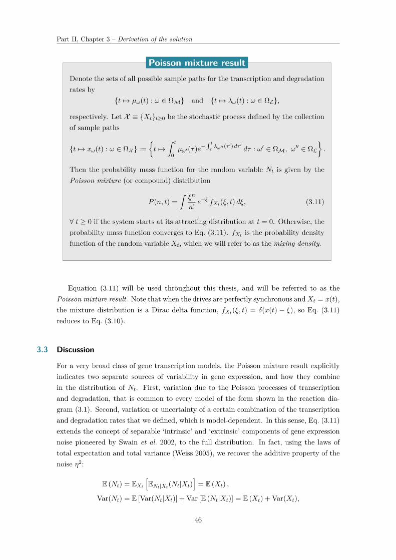
Part II, Chapter 3 – Derivation of the solution
Denote the sets of all possible sample paths for the transcription and degradationrates by
t 7→ µω(t) : ω ∈ ΩM and t 7→ λω(t) : ω ∈ ΩL,
respectively. Let X ≡ Xtt≥0 be the stochastic process defined by the collectionof sample paths
t 7→ xω(t) : ω ∈ ΩX ..=t 7→
∫ t
0µω′(τ)e−
∫ tτλω′′ (τ ′) dτ ′ dτ : ω′ ∈ ΩM, ω′′ ∈ ΩL
.
Then the probability mass function for the random variable Nt is given by thePoisson mixture (or compound) distribution
P (n, t) =∫ξn
n! e−ξ fXt(ξ, t) dξ, (3.11)
∀ t ≥ 0 if the system starts at its attracting distribution at t = 0. Otherwise, theprobability mass function converges to Eq. (3.11). fXt is the probability densityfunction of the random variable Xt, which we will refer to as the mixing density.
Poisson mixture result
Equation (3.11) will be used throughout this thesis, and will be referred to as thePoisson mixture result. Note that when the drives are perfectly synchronous andXt = x(t),the mixture distribution is a Dirac delta function, fXt(ξ, t) = δ(x(t) − ξ), so Eq. (3.11)reduces to Eq. (3.10).
3.3 Discussion
For a very broad class of gene transcription models, the Poisson mixture result explicitlyindicates two separate sources of variability in gene expression, and how they combinein the distribution of Nt. First, variation due to the Poisson processes of transcriptionand degradation, that is common to every model of the form shown in the reaction dia-gram (3.1). Second, variation or uncertainty of a certain combination of the transcriptionand degradation rates that we defined, which is model-dependent. In this sense, Eq. (3.11)extends the concept of separable ‘intrinsic’ and ‘extrinsic’ components of gene expressionnoise pioneered by Swain et al. 2002, to the full distribution. In fact, using the laws oftotal expectation and total variance (Weiss 2005), we recover the additive property of thenoise η2:
E (Nt) = EXt[ENt|Xt(Nt|Xt)
]= E (Xt) ,
Var(Nt) = E [Var(Nt|Xt)] + Var [E (Nt|Xt)] = E (Xt) + Var(Xt),
46

3.3. Discussion
soη2 = Var(Nt)
E (Nt)2 = 1E (Nt)
+ Var(Xt)E (Xt)
= η2int + η2
ext.
Note that the Poisson mixture result as an extension of the concepts of intrinsic andextrinsic noise emerged naturally from our initial assumptions, as did the relevant param-eter combination Xt to describe the extrinsic noise explicitly. We can use the Poissonmixture result to simplify analysis and explain properties of models in the same way asintrinsic and extrinsic noise components have (Elowitz et al. 2002; Volfson et al. 2006;Taniguchi et al. 2010). The problem of solving and analysing master equation models ofgene transcription is reduced to the problem of obtaining and studying only the variationthat is model-dependent, given by the mixing distribution fXt . This ability to discard the“Poisson part” of the model until we need it confers to us significant simplifications andadvantages compared to working with the full distribution P (n, t), not least because Xt
is a continuous random variable. In Chapter 4 we collect together some tools and meth-ods available to us for obtaining fXt analytically or numerically, and note how the costof stochastic simulations can be significantly reduced with the knowledge of Eq. (3.11).Similarly, obtaining moments and expressions for the noise become simple corollaries ofthe Poisson mixture result, as we will show in Chapter 5. Less obvious advantages becomeclear in Part III, where studying fXt instead of P (n, t) gives us a far deeper understandingof the models and their properties.
Let us begin.
47

Part II, Chapter 3 – Derivation of the solution
48

Chapter 4
On the mixture density fXt
We showed in Chapter 3 that for transcription-degradation models the distribution P (n, t)for the number of mRNA molecules at time t is given by the mixture density
P (n, t) =∫ξn
n! e−ξ fXt(ξ, t) dξ.
The challenge of obtaining P (n, t) is thus reduced to the task of obtaining the mixingdensity fXt , which contains all the model-specific properties of the solution.
We start this chapter by giving some intuition for how sample paths of the stochasticprocess X relate to sample paths for N , and how they relate to differential rate equationsused in ordinary differential equation (ODE) models of gene expression. We then collecttogether more general results from several fields that can aid us to determine fXt .
4.1 Physical interpretations and intuition
Before we look at methods for obtaining fXt , let us first try to gain some intuition viasome simple examples that:
• For a particular cell with extrinsic parameter xω(t)t≥0, xω(t) is a priori the ex-pected value of ηω(t), the sample path for the mRNA copy number for that cell attime t;
• the more synchronous or correlated the drives are in the population, the less dispersedthe distribution fXt will be (and hence the less dispersed P (n, t) will be);
• given the mean value E (Nt) = x for a population at time t, the Poisson distributionwith parameter x is the least dispersed possible distribution for P (n, t).
4.1.1 Static cell-to-cell correlations
Let’s consider a gene with sinusoidal transcription rate. This type of behaviour hasbeen observed for genes linked to circadian or cell cycles (Lück and Westermark 2015;Bieler et al. 2014), genes responding to cAMP signalling (Corrigan and Chubb 2014), andexternally-driven gene expression (Larson et al. 2013; Olson et al. 2014), for example. Aswe did in Chapter 3, we’ll first consider the case where the transcription and degradationrates are perfectly correlated for all cells, and then see how variability in the rates affectsthe extrinsic parameters and the distribution P (n, t).
49

Part II, Chapter 4 – On the mixture density fXt
Without extrinsic variation
Let us assume that the transcription rate is perfectly synchronous between all cells in thepopulation: every cell has transcription rate (Lück et al. 2014)
µ(t) ..= m[cos(θt) + 1]/2,
say. We can then easily calculate the extrinsic parameter x : t 7→ x(t) using its definition(Eq. (3.5)), which in this hypothetical scenario is deterministic. With λ ≡ 1 we have:
x(t) ..=∫ t
0µ(τ)e−(t−τ) dτ.
Since Xt = x(t) ∀ t, the density of Xt is given by
fXt(ξ, t) = δ(ξ − x(t)),
where δ is the Dirac delta function (Fig. 4.1, left column).
Despite knowing the drives precisely, transcription and degradation are still stochasticprocesses so each cell i in the population will have a different sample path ηi for the mRNAcopy number. We showed in Section 3.2 that in this special case with synchronous drives,at all times t, Nt = ηi(t) is distributed according to a Poisson distribution with meanx(t). In other words, if we took a snapshot of the population at time t and recorded thedistribution of the copy numbers, we would find that
P (n, t) = P (n, t|µ, λ) = xn(t)n! e−x(t).
Exemplary sample paths of N with the resulting distribution P (n, t) = P (n, t|µ, λ) areshown in Fig. 4.1, left column.
With extrinsic variation
Now suppose we extend the model to account for random cell-to-cell variation by assumingthat the transcription rates within the population are not completely synchronized. Weallow the phase Φ to be a random variable with some probability density that we maychoose, i.e.,
µi(t) = m[cos(θt+ φi) + 1]/2.
If we now pick a cell i at random from the population at time t, we do not know preciselywhat the value of its extrinsic parameter xi(t) will be; it is an outcome from a randomvariable Xt that has non-zero variance. The density fXt , which we derive in Example 4.2–1, will depend on the density of Φ. In turn, the distribution of Nt will be given by thePoisson mixture
P (n, t) =∫ m
0
ξn
n! e−ξfXt(ξ, t) dξ,
50

4.1. Physical interpretations and intuition
Figure 4.1: The effects of synchrony on a toy model with sinusoidal transcription rate,period T . Derivation of fXt is treated in Example 4.2–1. Left column: Synchronous drive,all heterogeneity is due to the Poisson processes of transcription and degradation. Thegraph for fXt for this synchronous case is a representation of a Dirac delta distributionwith mass at x(t) at time t. The snapshot distributions shown in the graph for P (n, t) arePoisson with mean x(t). Middle and right columns: The phase is uniformly distributedon an interval of range T/2 (middle), and T (right). Sample paths of the cellular driveX (top row), corresponding distribution fXt (second row), sample paths of the number ofmRNA molecules N (third row), and the exact solution P (n, t) (bottom). Throughout wehave taken m = 20.
which will necessarily be wider than a Poisson distribution to account for our uncertaintyin the extrinsic parameter. In Fig. 4.1 we show some sample paths xi(t) and ηi(t) alongwith fXt and P (n, t), when Φ is uniformly distributed on intervals of range T/2 andT , where T is the period. It is clear to see how decreasing the degree of synchrony ofthe cellular drives in the population increases the width of fXt and P (n, t). When thedrives are completely asynchronous, i.e. Φ ∼ Unif[−T/2, T/2], the model shows no timedependence: we have P (n, t) = P (n) ∀ t.
4.1.2 Dynamic cell-to-cell correlations
To give a better idea of how µ, λ, and x are related, let’s consider an example with a discretetranscription rate where the degree of synchrony (cell-to-cell correlation) fluctuates overtime. Suppose that for each cell i and at all times t we are able to keep track of themRNA copy number ηi(t) during the experiment. Assume also for the purposes of thissubsection that we are able to precisely control the transcription rate over time for singlecells, for example using light activation (Larson et al. 2013; Olson et al. 2014). For alltimes t when the light is on (resp. off), the transcription rate for all cells under the lightsource is µ(t) = m min−1 (resp. µ(t) = 0 min−1), say. At all times, the transcription rateis λ(t) = 1 min−1 per mRNA molecule.
51

Part II, Chapter 4 – On the mixture density fXt
0
5
10
15
200 0.3
0
5
10
15
200 0.3
0
5
10
15
200 0.3
ON ONOFF OFFON ON ... ON ONOFF OFFON ON ...
(a)
(b) (d)
(c)
Figure 4.2: Sample paths and probability distributions for a model with temporal controlof the transcription rate. (a, b) Immediate response of the transcription rate to the externalcontrol mechanism (light sequence) in all cells. (a) Time series of the light sequence, thetranscription rate µ (blue) and the corresponding extrinsic parameter x (black) that applyto every cell in the population. Hence fXt(ξ, t) = δ(ξ − x(t)) (representation omitted).Sample paths for the number of mRNA transcripts N are shown by the coloured lines. (b)Corresponding distribution P (n, t|µ, λ ≡ 1) over time, with x shown in black as a guide.A cross-section of the figure at any time ti would show the probability mass function ofa Poisson distribution with mean x(ti). (c, d) Response times to changes in the externalcontrol mechanism (light sequence) are exponentially distributed. (c) Sample paths of thetranscription rate (solid lines) and the corresponding extrinsic parameter (dashed lines).Sample paths of N have been omitted to maintain clarity. Inset: The density fXti fortimes ti indicated by the vertical dotted lines, to give an idea of its dynamic behaviour overtime. (d) Corresponding distribution P (n, t) over time, with sample paths of X shown asa guide. Cross-sections are now Poisson mixture distributions. Throughout we have takenm = 20.
Without extrinsic variation
Suppose that we have pre-programmed the light sequence so we have a population withperfectly synchronous drives µ : t 7→ µ(t) ∈ 0,m and λ : t 7→ 1 that we know precisely.As always, each cell i in the population will have a different sample path ηi for the mRNAcopy number. The trajectories ηi : t 7→ ηi(t) “follow” the extrinsic parameter x : t 7→ x(t),fluctuating around it. As before, the distribution of the ηi is a Poisson distribution withmean x(t), since the mixing density is fXt(ξ, t) = δ(ξ−x(t)). This will always be the casefor a population with perfectly synchronous drives, but in this example it is particularlyclear to see when looking at sample paths (Fig. 4.2a). Notice also that although thetranscription rate µ is discrete, x is a continuous function of time.
With extrinsic variation
Now suppose that when the light is turned on or off, there is a stochastic delay beforethe transcription rate responds; the switch is no longer synchronised. For each cell i, the
52

4.1. Physical interpretations and intuition
sample path µi is slightly different, particularly in the period immediately following thechange in the light, and it follows that the same will be the case for the sample pathsxi. Now, if we pick a cell i at random from the population at time t, we do not knowprecisely what the value of its extrinsic parameter xi(t) will be; it is an outcome from arandom variable Xt that now has non-zero variance. The density fXt will depend on thedensity of the response times to the light switching, and will be time-dependent (see theinsets of Fig. 4.2c). In turn, the distribution of Nt will again be given by the Poissonmixture, which will be more dispersed than a Poisson distribution. However, this timethe dispersion will fluctuate according to the dispersion of fXt (see Fig. 4.2c,d). fXt willbe most dynamic immediately after a change in the light sequence, since that is when thedistribution of the random variable Mt for the transcription rates will be evolving. Givena long enough waiting time between changes of the light sequence, the sample paths xiwould become almost indistinguishable, with values approaching m when the light is on,and zero when the light is off. As time increases without a switch in the light sequence,fXt would tend towards a delta distribution with mass at m or zero, and hence P (n, t)would tend towards a Poisson distribution with mean m or zero.
4.1.3 Relationship to ODE models of gene transcription
In chemical reaction kinetics it is common to approximate the number of molecules Nt bya continuous variable, or equivalently, to work in terms of its concentration. Given thereaction rates, we can then write down the differential rate law: an ordinary differentialequation that describes how the concentration varies in time. Here we will show how thedifferential rate laws for gene transcription models of the form (3.1) are related to themixing density fXt .
Denote the concentration of mRNA molecules in our cell population at time t by x(t).Suppose we know that the transcription rate is µ(t) and the degradation rate is λ(t).Under the assumptions laid out at the beginning of Chapter 3, transcription is a zeroorder reaction and degradation is a first order reaction. Hence the differential rate law is
dx
dt= µ(t)− λ(t)x(t). (4.1)
Importantly, this is precisely the equation we obtain by differentiating our integral defini-tion of x(t) (Eq. (3.5)).
Following the same reasoning as in Chapter 3 and the previous subsection, we canextend the use of the differential rate equation further to account for cell-to-cell variabilityor uncertainty in the reaction rates, or stochastic rates. Any sample paths t 7→ µω(t) andt 7→ λω(t) satisfy the differential rate equation (4.1), in turn defining the sample patht 7→ xω(t). For each t, the collection of all possible values xω(t) : ω ∈ ΩX defines ourrandom variable Xt, and the collection of all such ordinary differential equations can be
53
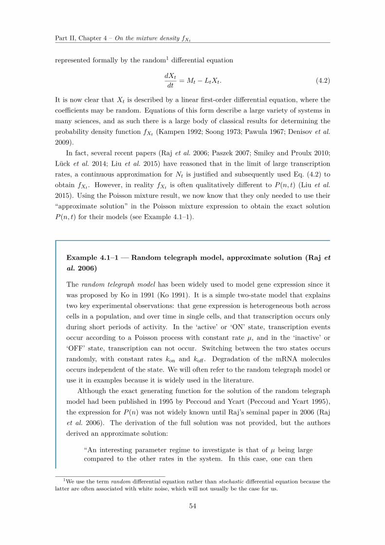
Part II, Chapter 4 – On the mixture density fXt
represented formally by the random1 differential equation
dXt
dt= Mt − LtXt. (4.2)
It is now clear that Xt is described by a linear first-order differential equation, where thecoefficients may be random. Equations of this form describe a large variety of systems inmany sciences, and as such there is a large body of classical results for determining theprobability density function fXt (Kampen 1992; Soong 1973; Pawula 1967; Denisov et al.2009).
In fact, several recent papers (Raj et al. 2006; Paszek 2007; Smiley and Proulx 2010;Lück et al. 2014; Liu et al. 2015) have reasoned that in the limit of large transcriptionrates, a continuous approximation for Nt is justified and subsequently used Eq. (4.2) toobtain fXt . However, in reality fXt is often qualitatively different to P (n, t) (Liu et al.2015). Using the Poisson mixture result, we now know that they only needed to use their“approximate solution” in the Poisson mixture expression to obtain the exact solutionP (n, t) for their models (see Example 4.1–1).
Example 4.1–1 — Random telegraph model, approximate solution (Raj etal. 2006)
The random telegraph model has been widely used to model gene expression since itwas proposed by Ko in 1991 (Ko 1991). It is a simple two-state model that explainstwo key experimental observations: that gene expression is heterogeneous both acrosscells in a population, and over time in single cells, and that transcription occurs onlyduring short periods of activity. In the ‘active’ or ‘ON’ state, transcription eventsoccur according to a Poisson process with constant rate µ, and in the ‘inactive’ or‘OFF’ state, transcription can not occur. Switching between the two states occursrandomly, with constant rates kon and koff . Degradation of the mRNA moleculesoccurs independent of the state. We will often refer to the random telegraph model oruse it in examples because it is widely used in the literature.
Although the exact generating function for the solution of the random telegraphmodel had been published in 1995 by Peccoud and Ycart (Peccoud and Ycart 1995),the expression for P (n) was not widely known until Raj’s seminal paper in 2006 (Rajet al. 2006). The derivation of the full solution was not provided, but the authorsderived an approximate solution:
“An interesting parameter regime to investigate is that of µ being largecompared to the other rates in the system. In this case, one can then
1We use the term random differential equation rather than stochastic differential equation because thelatter are often associated with white noise, which will not usually be the case for us.
54

4.2. Obtaining fXt using the differential equation for Xt
make the approximation that N is a continuous variable, X†. With thisapproximation, the dynamics can be described by
dX
dt= −λX + µr(t)
Here, r(t) ∈ 0, 1 is a random telegraph signal representing the active andinactive states of the gene.”
They go on to derive the steady-state probability density function for this approxima-tion, which is a scaled Beta distribution:
P (n) ≈ fX(x) =(µ
λ
)1− konλ− koff
λ Γ(konλ + koff
λ
)Γ(konλ
)Γ(koffλ
) x konλ−1(µ
λ− x
) koffλ−1
(4.3)
where kon and koff are the rates of switching on and off, resp.However, this approximation is precisely the mixture distribution required to write
down the exact solution as a Poisson mixture. Therefore, using the Poisson mixtureresult (3.11) the exact solution of the random telegraph model is:
P (n) =∫ µ/λ
0
ξn
n! e−ξ fX(ξ) dξ
=(µ
λ
)1− konλ− koff
λ Γ(konλ + koff
λ
)Γ(konλ
)Γ(koffλ
) ∫ µ/λ
0
ξn
n! e−ξ ξ
konλ−1(µ
λ− ξ
) koffλ−1
dξ (4.4)
=Γ(konλ + n
)Γ(konλ
) Γ(konλ + koff
λ
)Γ(konλ + koff
λ + n) (µλ)n
n! F1 1
(konλ
+ n,konλ
+ koffλ
+ n;−µλ
),
where F1 1 is the confluent hypergeometric function (Abramowitz and Stegun 1964).The last line is the form of the exact solution that was stated in the supplementarymaterial of (Raj et al. 2006), but was not derived. It can be deduced from the Poissonmixture form using a standard integral representation of the confluent hypergeometricfunction (Abramowitz and Stegun 1964).†Notation changed from the original text to be consistent with the notation used in this thesis.
Note that, unlike the approximation to a continuous variable, we do not need to make anyassumptions about the value of any parameters to obtain the exact solution.
4.2 Obtaining fXt using the differential equation for Xt
Obtaining the distribution of a random variable can be difficult if not impossible, andusually requires one to solve an equation for the density function explicitly. However,
55

Part II, Chapter 4 – On the mixture density fXt
since our random variable Xt satisfies the simple, first-order linear differential equation
dXt
dt+ LtXt = Mt, (4.5)
we can sometimes obtain the density function fXt more directly. Here we give two ex-amples: first, when the solution Xt of Eq. (4.5) is an invertible function of a randomvariable which we know the distribution of, and second, when we do not require (or cannot otherwise obtain) an explicit expression for fXt and need to resort to cost-effectivesimulations.
4.2.1 Obtaining fXt via a change of variablesIf we solve the formal differential equation for Xt directly and find that it can be writtenin the form
Xt = g(Φt),
where Φt is a random variable whose probability density we know, we can calculate fXtusing standard techniques for transformations of random variables. Suppose the transfor-mation g is “nice enough” that the preimage g−1(x) = φ : g(φ) = x is countable for anyx in the range of Xt. We can then obtain the cumulative distribution function FXt or theprobability density function fXt from first principles. When g is injective, φ ..= g−1(x) isunique and the procedure is fairly straightforward:
FXt(x, t) = Pr(Xt ≤ x)
= P (g(Φt) ≤ x)
= P (Φt ≤ g−1(x))
= FΦt(g−1(x), t)
= FΦt(φ, t),
and
fXt(x, t) = d
dxFXt(x, t)
= fΦt(g−1(x), t)∣∣∣∣∣dg−1(x)
dx
∣∣∣∣∣= fΦt(φ, t)
∣∣∣∣ 1g′(φ)
∣∣∣∣ .When g is not injective, the same steps can be taken but extra care is required. Theclearest way to demonstrate is with an example.
56

4.2. Obtaining fXt using the differential equation for Xt
Example 4.2–1 — Sinusoidal transcription rate with distributed phase
Consider the toy model discussed at the beginning of this chapter, where the tran-scription rate in each cell is sinusoidal with a distributed phase Φ:
Mt..= m[cos(θt+ Φ) + 1]/2,
and constant degradation rate λ ≡ 1.Solving Eq. (4.5) and ignoring the effects of initial conditions for simplicity, we
obtain
Xt = m
2(1 + θ2)[1 + θ2 + cos(θt+ Φ) + θ sin(θt+ Φ)
]= B +A sin(θt+ Φa),
where A ..= m/2√
1 + θ2, B ..= m/2 and Φa..= Φ + arctan(1/θ). Then,
FXt(x, t) ..= P (Xt ≤ x)
= P
(sin(θt+ Φa) ≤
x−BA
).
Now, the set of intervals[φ1, φ2] : ∀ ψ ∈ [φ1, φ2] , sin(θt+ ψ) ≤ x−B
A
is countable, so we may proceed. Suppose for example that Φa is uniformly distributedon the interval [−r, r], with r ≤ π. It is then easy to show that
FXt(x, t) = s(t)2r arcsin
(x−BA
)+ terms independent of x,
where s(t) ∈ 0, 1, 2 is the number of solutions of
sinϕ = x−BA
, ϕ ∈ (θt− r, θt+ r).
Differentiating, we finally obtain
fXt(x, t) = s(t)2r√A2 − (x−B)2
= s(t)2r
([m
2(1 + θ2)
]2−[x− m
2
]2)− 1
2
(see Fig. 4.1, second row). Clearly, as r tends to zero, i.e. the phase difference betweenany two cells tends to zero, fXt(x, t) tends to the Dirac delta function centred at
57

Part II, Chapter 4 – On the mixture density fXt
B + A sin(θ t). Substituting back into the Poisson mixture solution in this limit werecover the Poisson solution for the case of a synchronous population, as expected (seeFig. 4.1, left column):
P (n, t) = x(t)n e−x(t)
n!= 1n! [B +A sin(θ t)]n e−[B+A sin(θ t)]
4.2.2 Reduction of simulation costsAn explicit expression for P (n, t) is difficult to obtain for all but a handful of gene transcrip-tion models. Even with the Poisson mixture result and the tools to obtain fXt analyticallythat are presented in the rest of this chapter, one can not always obtain an exact, practicalexpression for P (n, t).
Several approximation methods have been proposed to approximate P (n, t) (Kam-pen 1992; Munsky and Khammash 2006; Thomas et al. 2012), but probably the moststraightforward, popular approach is to use a stochastic simulation algorithm to gener-ate sample paths of the model in question (Gillespie 1976; Gillespie 1977; Cao et al.2006). The distribution of the sample paths can then be used as an approximation forthe theoretical probability distribution P (n, t), with the approximation approaching thetheoretical one in the limit of infinite sample paths. Although this approach is simple, canbe applied to complex systems, and does not require any equations to be solved, it canbe extremely computationally expensive and can fail dramatically when time-dependentrates are used (Voliotis et al. 2015).
However, the Poisson mixture result tells us that we need only obtain fXt , and thenperform the mixture. Simulating sample paths of X instead of N can drastically decreasesimulation costs, as we do not need to consider the stochastic processes of transcription ordegradation explicitly. We are then balancing the costs of simulating ηω(t) : t ≥ 0 fromxω(t) : t ≥ 0, versus performing some numerical integration to obtain P (n, t) from fXt .
Example 4.2–2 — Stochastic simulations for the multistate “Ladder” model
Consider an extension of the random telegraph model where the gene may switchbetween three different gene states in a ladder structure, as shown in Fig. 4.3 (Senecalet al. 2014). The transcription rate is modelled by a continuous-time Markov chainwith state space 0, µ1, µ2, µ1 < µ2, corresponding to the states OFF,ON1,ON2,respectively. The degradation rate λ is a constant and independent of gene state.
An exact solution for this model is not known†, but obtaining an approximation for
58

4.3. Kramers-Moyal equation for fXt
fXt via stochastic simulations is extremely quick because X is a piecewise-deterministicMarkov process (Davis 1984). In other words, the behaviour of the sample paths xω isgoverned by the random jumps between gene states at countable times ti, but in be-tween those times the value of xω evolves deterministically according to the ODE (4.1)(see Fig. 4.3 for an sample path of X ). Assuming that the cells are uncoupled, thesystem is ergodic so we can simulate one sample path xω(t)t∈[0,T ] and compute atime average (see Section 5.2), which will tend to the exact solution as T → ∞ ifsimulated for example according to the Gillespie algorithm (Gillespie 1977). The sta-tionary solution P (n) can then be obtained by performing the Poisson mixture withthe approximation for fX , via numerically integration.
Without knowledge of the Poisson mixture result and the differential rate equa-tion (4.1) for the sample paths of X , we would need to use the Markov chain for thegene state to simulate a sample path of N . In this case we need to obtain event timesfor every transcription and degradation event, as well as the gene state switching times,so in general the costs will be much higher than the method described above.
Time average
mRNA
mRNA
(a) (b) (c)
Figure 4.3: Approximating fX via stochastic simulations. (a) Three-state Laddermodel of gene transcription. The gene switches between an inactive state (OFF)and two active states (ON1 and ON2), with transition rates indicated in the figure.Transcription takes place according to a Poisson process with rate µ1 in ON1 andµ2 > µ1 in ON2. Degradation of transcripts occurs stochastically with rate λ permolecule per unit time. (b) Sample path of X , using biologically realistic parametervalues (Senecal et al. 2014). The gene state is indicated by pink (OFF), light green(ON1), and dark green (ON2) shading. (c) The resulting stationary probability densityfX .
†However, in Chapter 7 we show that fXt satisfies Heun’s equation (Ronveaux 1995).
The cost reduction is particularly noteworthy when we do not have an ergodic2 system,because millions of simulations are required to obtain enough data for a reliable probabilitydistribution of Nti at each time point ti.
4.3 Kramers-Moyal equation for fXt
Although X ≡ Xtt≥0 satisfies a simple linear equation, when both M ≡ Mtt≥0
and L ≡ Ltt≥0 are stochastic processes expressions can quickly become intractable.2See Section 5.2 for a definition of ergodicity and the implications this has for obtaining solutions.
59

Part II, Chapter 4 – On the mixture density fXt
See Soong 1973 for a readable introduction to the theory and results for these kinds ofdifferential equation. Fortunately, in terms of the transcription and degradation of mRNAmolecules it has been shown that most of the variability in N comes from the dynamics atthe promoter (Coulon et al. 2010; Suter et al. 2011; Carey et al. 2013; Sánchez and Golding2013). Indeed, frequently the degradation probability is approximately constant (Raj et al.2006; Harper et al. 2011; Suter et al. 2011) and in this case fXt can often be determined.
Taking L ≡ λ = constant, the differential equation for Xt (Eq. (4.2)) becomes anordinary differential equation with a random inhomogeneous part, which can be consideredas the output of a dynamical system governed by a simple first-order ordinary differentialequation with random drive Mt. Equations of this form have been studied since 1908when Paul Langevin investigated Brownian motion, and are still of paramount importancefor applications in fields as wide as electrical engineering, neuroscience, civil engineering,communication theory, economics and finance, and biology (Langevin 1908; Zon et al. 2004;Fitzhugh 1983; Crandall and Zhu 1983; Rolski et al. 2009). As such, there is a large bodyof results relating to ordinary differential equations with a random drive. Importantly,the following classical results (Kramers 1940; Moyal 1949) provide us with a differentialequation for fXt , and some general properties. We demonstrate a brief derivation of thedifferential equation for completeness.
Let fXt be the probability density function of the random variable Xt that satisfies
dXt
dt+ λXt = Mt, (4.6)
where Xtt≥0 and Mtt≥0 are continuous-time processes, Xt can take a continuum ofvalues, and λ is a constant. Denoting the conditional density for Xt+∆t = x given thatXt = x′ by fXt+∆t|Xt(x, t+ ∆t|x′, t), the Markov property gives us
fXt+∆t(x, t+ ∆t) =∫ ∞−∞
fXt+∆t|Xt(x, t+ ∆t | x′, t) fXt(x′, t) dx′. (4.7)
Now consider the conditional characteristic function φ of the random variable ∆Xt..=
Xt+∆t −Xt given that Xt = x′:
φ(u, t+ ∆t|x′, t) = E(eiu∆X
∣∣∣x′, t)=∫ ∞−∞
eiu∆x fXt+∆t|Xt(x, t+ ∆t|x′, t) dx,
where ∆x ..= x − x′. Perform the inverse Fourier transform and expand φ(u, t + ∆t|x′, t)in a Taylor series around u = 0:
fXt+∆t(x, t+ ∆t|x′, t) = 12π
∫ ∞−∞
e−iu∆x φ(u, t+ ∆t|x′, t) du
=∞∑n=0
an(x′, t)2πn!
∫ ∞−∞
(iu)n e−iu∆x du
60

4.3. Kramers-Moyal equation for fXt
=∞∑n=0
(−1)nn! an(x′, t) dn
dxnδ(∆x), (4.8)
wherean(x′, t) ..= 1
in∂nφ
∂un
∣∣∣∣u=0
= E([∆Xt]n|x′, t
).
Substituting Eq. (4.8) into Eq. (4.7) and performing the integration by parts, we obtain
fXt+∆t(x, t+ ∆t) =∞∑n=0
(−1)nn!
∂n
∂xn[an(x, t) fXt(x, t)]
= fXt(x, t) +∞∑n=1
(−1)nn!
∂n
∂xn[an(x, t) fXt(x, t)].
Finally, putting fXt(x, t) on the left hand side, dividing by ∆t and taking the limit ∆t→ 0gives the Kramers-Moyal equation:
∂fXt(x, t)∂t
=∞∑n=1
(−1)nn!
∂n
∂xn[αn(x, t)fXt(x, t)], (4.9)
whereαn(x, t) ..= lim
∆t→0
1∆tE ([Xt+∆t −Xt]n | Xt = x) , n = 1, 2, . . . (4.10)
We will refer to the αn as the jump moments, although they are sometimes known as theKramers-Moyal moments, or derivate moments. Similarly, the Kramers-Moyal equationis sometimes referred to as the kinetic equation associated with the stochastic processX † (Soong 1973).
4.3.1 The Fokker-Planck equation can only be an approximationThe Kramers-Moyal equation (4.9) is, a priori, a partial differential equation of infiniteorder. However, Pawula (Pawula 1967) showed that in fact it is either of infinite order, orit is of order at most two:
If αn <∞ ∀ n and if αn = 0 for some even n, then
αn = 0 ∀ n ≥ 3. (4.11)
In the finite case, Eq. (4.9) becomes the well-known Fokker-Planck equation, sometimescalled the Kolmogorov forward equation:
∂fXt∂t
= − ∂
∂x(α1fXt) + 1
2∂2
∂x2 (α2fXt) .
Clearly, when solving a gene transcription model one would rather be in the positionwhere fXt satisfies the Fokker-Planck equation, instead of the infinite order Kramers-†Note that the Kramers-Moyal equation (4.9) is (in general) a partial differential equation of infinite
order, in one dimension. It is thus different from the multidimensional Fokker-Planck equation, which is asecond-order partial differential equation in several dimensions.
61

Part II, Chapter 4 – On the mixture density fXt
Moyal equation. An interesting question, then, is to ask for what kind of process Xcan we obtain the full statistical description by solving only the Fokker-Planck equation?Physically, αn = 0 for n ≥ 3 implies that X can only change by a small amount in a smalltime interval: E ([X(t+ ∆t)−X(t)]n) approaches zero faster than ∆t as ∆t→ 0. To ourknowledge, no one has yet been able to fully characterise all stochastic processes X thatsatisfy this condition. However, a sufficient constraint is that X be a continuous Markovprocess - for a proof see for example (Gillespie 1992b; Risken 1989).
Now, ifM has stationary, independent increments, X is a Markov process. However,sinceM does not depend on X in our framework, the only example where X is a continuousMarkov process is the Ornstein-Uhlenbeck process, whereM is a white Gaussian process.This assumption implies that there is a non-zero probability that X will become negative,and hence it can not be part of a physical model of gene transcription. In other words,no physical model of gene transcription will enjoy having a stochastic process X whosestatistical properties are fully described by the Fokker-Planck equation. Nevertheless, sincethe Ornstein-Uhlenbeck process is the only example where the Fokker-Planck equationwould result in an exact solution, we include it to give an intuition as to how X fits inwith more well-known frameworks from the physics literature.
Example 4.3–1 — When X is a continuous Markov process
Suppose the degradation rate L ≡ λ is a constant, and the transcription rateM is aconstant µ with an added noise term, which is normally distributed. Then Xt satisfiesthe Ornstein-Uhlenbeck equation
dXt = λ
(µ
λ−Xt
)+ σdWt,
where σ > 0 is the standard deviation of the noise andWt denotes the Wiener process.fXt then satisfies the Fokker-Planck equation
∂fXt∂t
= −λ ∂
∂x
[(µ
λ− x
)fXt
]+ σ2
2∂2fXt∂x2 ,
with solution
fXt(x, t|X0 = x0) =exp
−[x−µ
λ−e−λt(x0−µλ )]2
σ2(1−e−2λt)/λ
√πσ2(1− e−2λt)/λ
.
HenceXt ∼ N
(µ
λ+ e−λt
(x0 −
µ
λ
),σ2
2λ(1− e−2λt
)).
62

4.4. Multistate Kramers-Moyal equation
One might hope that a higher order truncation of the Kramers-Moyal equation wouldyield a good approximate solution for fXt . Unfortunately, a naïve truncation is not alegitimate procedure (Risken 1989; Kampen 1992; Plyukhin 2008) as it can prescribenegative values for fXt and give a worse approximation than truncation at order two.A system-size expansion as pioneered by van Kampen (Kampen 1992) can yield betterapproximations (Grima et al. 2011).
4.4 Multistate Kramers-Moyal equation
The Kramers-Moyal equation (4.9) in theory provides a means for obtaining fXt . However,as explained in the previous section this partial differential equation will always be ofinfinite order for realistic models of gene transcription. In addition, the steady-stateKramers-Moyal equations will be degenerate for certain choices of transcription processes,including the important class of multistate promoter models (Pawula 1967), which we willdefine and discuss in Part III. Fortunately, by extending our state space the Kramers-Moyal equation can be extended to account for multistate models, giving a system ofdifferential equations.
In this section we present the multistate Kramers-Moyal equations, and apply them tothe random telegraph model to demonstrate how easily the known solution for this modelcan be rederived using these results. We defer new results to Part III, where we describein detail how these systems of equations can be solved for more complex, as-yet unsolvedexamples, and how they can help us deduce which models are solvable.
Consider a multistate model where the promoter transitions between a set of J discretestates sjJj=1, each with its own transcription rateMj and degradation rate Lj . We needto consider the expanded state space Xt, St, where Stt≥0 is a discrete random processthat describes the promoter state. Our desired probability density function fXt is thengiven by
fXt(x, t) =∑j
fXt,St(x, sj , t),
with
∂
∂tfXt,St(x, sj , t) =
∞∑n=1
(−1)nn!
∂n
∂xn[αn(x, sj , t)fXt,St(x, sj , t)]
+J∑k=1
βk(x, sj , t)fXt,St(x, sk, t), (4.12)
whereαn(x, sj , t) = lim
∆t→0
1∆tE ([Xt+∆t −Xt]n | Xt = x, St = sj) (4.13)
are the jump moments as before, and
βk(x, sj , t) = lim∆t→0
1∆t [Pr(St+∆t = sj | Xt = x, St = sk, t)− δjk] , (4.14)
63
Part II, Chapter 4 – On the mixture density fXt
are the transition rates between states. δjk denotes the Kronecker δ-function (Pawula1967; Pawula 1970). We will refer to these as the multistate Kramers-Moyal equations. Ofcourse if we only have one state, there are no transition probabilities and the multistateKramers-Moyal equations (4.12) reduce to the standard Kramers-Moyal equations (4.9)from the previous section.
If the jump moments terminate and Stt≥0 is Markovian, then so too is the jointprocess Xt, Stt≥0 so Equations (4.12) are of finite order. Any model with constanttransition rates, as is most common in the literature, is of this type. Furthermore, unlessthe model uses white noise, α2j = 0 ∀ j = 1, . . . , J so the multistate Kramers-Moyalequations reduce to:
∂
∂tfXt,St(x, sj , t) = − ∂
∂x[α1(x, sj , t)fXt,St(x, sj , t)] +
J∑k=1
βjk(x, t)fXt,St(x, sk, t)
= − ∂
∂x[(µj(t)− λjx)fXt,St(x, sj , t)] +
J∑k=1
βjk(x, t)fXt,St(x, sk, t),
for j = 1, . . . , J .The most simple, well-known multistate promoter model is the random telegraph
model, which has two promoter states and constant parameters. As mentioned in Ex-ample 4.1–1, fXt for the random telegraph model was obtained as an approximation tothe full solution in the supplementary material of Raj et al. 2006. They did this by brieflyjustifying and solving the multistate Kramers-Moyal equations for this particular model,seemingly without being aware of Pawula’s more general results. In the following examplewe will show how to use the definitions of the jump moments (4.13) to write down thesesame equations to solve, but for the most general form of the random telegraph model. Forcompleteness, we then solve the simultaneous equations by substitution as shown in (Rajet al. 2006), although a more general method that dispenses of the need for substitutionby hand is presented in Chapter 6.
Example 4.4–1 — Random telegraph model with leaky transcription andstate-dependent degradation rates
Consider a 2-state model where the gene state transitions stochastically between anactive state son and an inactive state soff . Transcription occurs at rate µon in son, andinefficiently at rate µoff < µon in soff . Although degradation is usually assumed tooccur independently of promoter state, it does not complicate the derivations here ifwe allow the degradation rates λon and λoff in states son and soff , resp., to be distinct.
64

4.4. Multistate Kramers-Moyal equation
To simplify notation we will write
fXt(x, t) = fon(x, t) + foff(x, t), where
fon(x, t) ..= fXt,St(x, son, t), and
foff(x, t) ..= fXt,St(x, soff , t).
In order to write down the multistate Kramers-Moyal equations for fon and foff weneed to determine the jump moments αn for n ∈ N, and the transition rates β. Thelatter are simply the transition rates given in the model description:
βoff,on = lim∆t→0
1∆t [Pr(St+∆t = soff | Xt = x, St = son)− δoff,on]
= koff
βon,on = lim∆t→0
1∆t [Pr(St+∆t = son | Xt = x, St = son)− δon,on]
= −koff
and similarly, βon,off = kon and βoff,off = −kon.To determine the jump moments, first notice that in the derivation of the Kramers-
Moyal equation (4.9) the jump moments αn appear from the Taylor expansion of theconditional characteristic function, so we can write:
αn(x, t) = 1in
lim∆t→0
1∆t
∂nφ
∂un
∣∣∣∣u=0
(4.15)
For the multistate Kramers-Moyal equations the notation is slightly different, to ac-count for the expanded state space: we will need the jump moments αn,on and αn,off .They will satisfy this same equation above, Eq. (4.15), but the conditional character-istic function φ will be conditional on the state St as well as on Xt.
To find this conditional characteristic function φ, write Eq. (4.6) in difference form:
lim∆t→0
Xt+∆t −Xt
∆t = Mt − LtXt,
i.e.∆Xt = Mt∆t− LtXt∆t+ o(∆t),
where o(∆t) denotes terms that tend to zero faster than ∆t as ∆t → 0. Rememberthat in this random telegraph model the transcription rate and the degradation ratejump between two discrete values: Mt ∈ µon, µoff and Lt ∈ λon, λoff. Then wehave:
φ(u, t+ ∆t∣∣Xt = x, St = son) = E
(eiu∆Xt
∣∣∣Xt = x, St = son)
= E(eiu[Mt∆t−LtXt∆t+o(∆t)]
∣∣∣Xt = x, St = son)
65

Part II, Chapter 4 – On the mixture density fXt
= eiu[µon∆t−λonx∆t+o(∆t)],
and similarly
φ(u, t+ ∆t∣∣Xt = x, St = soff) = eiu[µoff∆t−λoffx∆t+o(∆t)].
Using the definition of the jump moment, Eq. (4.15), we find:
α1,on(x, t) = 1i
lim∆t→0
1∆t
∂
∂u
eiu[µon∆t−λonx∆t+o(∆t)]
∣∣∣u=0
= µon − λonx, and similarly
α1,off(x, t) = µoff − λoffx;
α2,on(x, t) = 1i2
lim∆t→0
1∆t
∂2
∂u2
eiu[µon∆t−λonx∆t+o(∆t)]
∣∣∣u=0
= 0, and similarly
α2,off(x, t) = 0.
Since the second jump moments are zero, we can immediately deduce using Eq. (4.11)that αn,on = 0 and αn,off = 0 ∀ n ≥ 2. Note that since the expanded state spaceXt, Stt≥0 is Markovian, finite multistate Kramers-Moyal equations were expectedanyway.
Putting this all together into the multistate Kramers-Moyal equations (4.12), andsetting the time derivatives equal to zero so that we obtain the steady-state solution,we finally obtain
d
dx[(µon − λonx)fon] = −kofffon + konfoff
d
dx[(µoff − λoffx)foff ] = kofffon − konfoff
These simultaneous ordinary differential equations can be solved straightforwardly bysubstitution, as shown in more detail in (Raj et al. 2006) for example. The finalsolution is then
fXt(x, t) = C(µon − λonx)koffλon−1(λoffx− µoff)
konλoff−1[(µon − µoff)− (λon − λoff)x] ∀ t,
where the constant of integration C can be determined with the integral condition∫ maxµon/λon, µoff/λoff
minµon/λon, µoff/λofffX(x) dx = 1.
When λon = λoff = λ, we obtain the usual solution for the leaky random telegraph
66

4.5. Equation for fXt using Fourier transforms
model (Smiley and Proulx 2010):
fXt(x, t) = λ(µon − λx)koffλ−1(λx− µoff)
konλ−1
(µ1 − µ0)kon+koff
λ−1B
(konλ ,
koffλ
) ,
where B is the beta function.
4.5 Equation for fXt using Fourier transforms
The differential equation (4.2) for Xtt≥0 can be thought of as a description of the timeevolution of a dynamical system that interacts with a randomly fluctuating environment.As such, in the field of statistical physics this equation would be called a Langevin equation(with a non-Gaussian noise termMt). Obtaining the probability density fXt of the solutionof a Langevin equation is often a primary concern to statistical physicists, so we are ableto draw on some of the results derived in that field to help us determine fXt .
For brevity, here we mention only one fairly recent result derived in Denisov et al.2008; Denisov et al. 2009, that provides an equation and some exact solutions for fXtin certain cases. Note that their results apply to a slightly different general setting thanwe are constrained to by Eq. (4.5), so the expressions that we include here are only thespecific cases of their original results that apply to our system. Additionally, for theirresults to hold we must assume that i) our degradation rate L ≡ λ is constant, and ii) Mt
can be written as the time derivative of the “noise generating process” Ξt, i.e.:
∆Ξt ..= Ξt+∆t − Ξt =∫ t+∆t
tMτ dτ.
Then, the increment ∆Xt..= Xt+∆t − Xt during a time interval of ∆t, ∆t → 0, can be
written in the form∆Xt = −λXt∆t+ ∆Ξt.
Write the probability density function of the random variable ∆Ξt as f∆Ξt(ξ,∆t), denoteits Fourier transform by f∆Ξt(k, t), and define
φk ..= lim∆t→0
1∆t
[f∆Ξt(k, t)− 1
],
which is a measure of the strength of the influence of Mt on the system. Denoting also byfXt(k, t) the Fourier transform of fXt(x, t), we have (Denisov et al. 2009)
fXt(k, t) = exp(− 1λ
∫ k
0
φze−λt − φzz
dz
),
67

Part II, Chapter 4 – On the mixture density fXt
or equivalently
fXt(x, t) = F−1
exp(− 1λ
∫ k
0
φze−λt − φzz
dz
), (4.16)
where F−1 is the inverse Fourier transform operator.
Example 4.5–1 — Poisson white noise: in the limit of infinitesimally shortburst intervals
Pedraza and Paulsson (Pedraza and Paulsson 2008) assumed that transcriptionalbursts occurred on timescales so short that they could be modelled by discrete jumpsin the sample paths of N (see Figure 4.4). They were able to obtain expressions forthe mean and variance of Nt in the stationary case, but using the Fourier transformmethod we can obtain a closed-form expression for P (n, t) for certain waiting time andburst size distributions.
0
10
20
30
40
Figure 4.4: Sample path of N for a model with Poisson white noise: random bursttimes ti occur according to a Poisson process with constant rate β, and the burst sizessi are drawn from a probability distribution q. Degradation of mRNA transcripts is afirst-order process with constant rate.
Suppose L ≡ λ and transcription only occurs during short “burst” intervals, withexponentially distributed waiting times between bursts. Suppose further that eachburst at time t increases the expectation of Nt by a random variable S, i.e. S describesthe burst size. In the limit of infinitesimally short burst times, the transcription ratecan be modelled by a Poisson sequence of Dirac delta pulses:
µω(t) =Bt∑i=1
si δ(t− ti),
where
Bt ∼ Poi(β) is a Poisson process that counts the bursts up to time t,
ti are the burst times of this Poisson process,
68
4.6. Discussion
si are independent outcomes from the random variable S
with probability density q,
δ(·) is the Dirac delta function.
In this caseφk = β(qk − 1),
where qk is the Fourier transform of the probability density of the burst sizes, sosubstitution into Eq. (4.16) gives
fXt(x, t) = F−1
exp(−βλ
∫ k
0
qze−λt − qzz
dz
). (4.17)
For certain choices of q we can evaluate Eq. (4.17) to give an explicit solution in termsof x and t only. For example, choosing the exponential distribution we have (Denisovet al. 2009)
q(s) = r
2e−rs, r, s > 0
so qk = r2
r2 + k2
and fXt(x, t) = F−1
exp(−βλ
∫ k
0
r2(1− e−2λt)z(r2 + z2)(r2 + z2e−λt) dz
)
= F−1
(r2 + k2e−2λt
r2 + k2
) β2λ .
Letting t→∞ we can invert the Fourier transform to obtain the stationary distribu-tion:
fX(x) =√
2π
r(rx)(β−λ)/2λ
2β/2λΓ(β2λ
) K(β−λ)/2λ(rx),
where K is the modified Bessel function of the second kind (Abramowitz and Stegun1964).
4.6 Discussion
As noted at the end of Chapter 3, the mixing density fXt is the essence of any transcription-degradation model of the kind we consider in this thesis. Before moving on to using thePoisson mixture result to derive solutions and properties of models, this chapter aimedto give some physical intuition for the extrinsic random variable Xt, and introduce somemethods one may use to obtain its density fXt . It is far from a complete exposition of theknown approaches to derive or approximate fXt , which would have taken us away fromthe scope of this thesis.
69

Part II, Chapter 4 – On the mixture density fXt
In particular, we could have dwelt far longer on the advantages afforded to us by thePoisson mixture result when obtaining numerical solutions. We stated in Section 4.2.2that approximating fXt using a stochastic simulation algorithm can be much quicker thanapproximating P (n, t), but a more detailed investigation would exemplify how significantthe savings can be.
70
Chapter 5
Averaging in space or time
The previous two chapters were concerned with obtaining the complete statistical descrip-tion P (n, t) = Pr(Nt = n) of the random process N = Ntt≥0. In general, this solutionwould give information about cell-to-cell heterogeneity of a population, as well as how thatis expected to change over time. However, in certain circumstances such detailed infor-mation may not be required or relevant, and simpler characterisations based on averagesare of more interest. This chapter uses what we know about the full distribution P (n, t)to derive some corollaries in this direction.
In particular, a fundamental question in the study of gene expression concerns thenature and origins of the heterogeneity due to stochastic processes, or “noise”, that isobserved so ubiquitously in this field. Noise is characterised using different metrics ac-cording to the type of data or model being analysed, but many of the most simple, intuitivemetrics use combinations of moments. These include the two that are most commonlyused for gene expression data: the coefficient of variation, η, (or the squared coefficient ofvariation, η2) (Elowitz et al. 2002; Swain et al. 2002; Paulsson 2005):
η ..= standard deviationmean , or η2 ..= variance
mean2 ,
and the Fano factor (Thattai and Oudenaarden 2001; Golding et al. 2005; Munsky et al.2012):
Fano factor ..= variancemean .
It is clear from the definitions that these metrics are very similar, and one is usuallychosen over the other based only on how easy they are to interpret in the given con-text. The coefficient of variation is a dimensionless quantity, so it gives a standardisedmeasure of dispersion. The Fano factor has been popularized more recently by van Oude-naarden (Thattai and Oudenaarden 2001; Raj and Oudenaarden 2009) specifically for thekinds of gene transcription models we consider here; under the assumption that thereis no gene regulation, transcription and degradation of mRNA are zero- and first-orderstochastic processes with constant rates µ and λ, say, and the stationary distribution ofN is a Poisson distribution with parameter µ/λ. The Fano factor equals one for a Pois-son distribution, so it is a useful measure of deviation from the constant-rate model ofunregulated gene expression.
Although it is rarely explicitly stated, Fano factor analysis of gene transcription dataor models so far have used ensemble moments in the definition (see below). However,
71

Part II, Chapter 5 – Averaging in space or time
the Fano factor was originally defined to characterise noise in time course data (Fano1947), using the mean and variance calculated over a time window (temporal moments,see below). We will refer to the Fano factor calculated using ensemble (resp. temporal)moments as the ensemble (resp. temporal) Fano factor, and discuss each separately in thecorresponding sections below, as they have very different interpretations and will not givethe same value.
Before we continue, let’s clarify what we mean by ensemble and temporal moments:under the general framework outlined in Chapter 3, the distribution P (n, t) has two di-mensions across which we may take an average. First, for each fixed t we can consider theensemble moments
E(Nkt
)..=∑n
nk P (n, t).
They correspond to averaging on a snapshot of the population at time t, and will betime-dependent if the statistical properties of the transcription and/or degradation ratesare. For example, mean expression levels of circadian genes exhibit approximately periodicbehaviour over 24-hour intervals (Bieler et al. 2014; Lück and Westermark 2015). Expres-sions for the ensemble moments and other corollaries will be discussed in Section 5.1.
Second, with single-cell time course data or ergodic models we can consider the temporalmoments
〈Nkt 〉 ..= 1
T
∫ T
0nk P (n, t) dt.
As the name suggests, temporal moments can allow us to compare the average expressionof single cells over a time interval, such as a cell cycle, duration of an experiment, or aftera change at the promoter. In addition, the temporal average can be used to derive analternative solution of the master equation for ergodic models which is especially usefulwhen we have periodic drives. All these concepts will be discussed in more detail inSection 5.2.
5.1 Ensemble moments
Ensemble moments hold an important place in gene expression analysis. Experimentalmethods such as northern blotting, microarrays, qPCR, and RNA-Seq are only capable ofobtaining the concentration or a measure of the total amount of a substance or molecule ina cell population, equivalent to the mean value of a population snapshot. Even with singlecell data, moments are useful quantitative characterisations of the data that can be usedfor comparisons or expression summaries. On the theoretical side, we showed in Chapter 3that the solution P (n, t) can always be written in Poisson mixture form, but if fXt can notbe determined or the integration is difficult this description might not be fit for purpose.On the other hand, expressions for the moments are usually easier to obtain and/or workwith, and can be used to approximate the full distribution if necessary (Lasserre 2002;Bertsimas and Popescu 2005). In addition, conclusions regarding gene expression noiseare usually based on the squared coefficient of variation or ensemble Fano factor (Paulsson
72

5.1. Ensemble moments
2004; Ozbudak et al. 2002; Thattai and Oudenaarden 2001).Our possession of the integral form of the solution (Eq. (3.11)) enables us to determine
the time-dependent moments E(Nkt ) from E (Xr
t )kr=1, and vice versa. We will firstderive these relations, and then use them to deduce properties of the ensemble noisecharacteristics.
5.1.1 Derivation of the ensemble moments of Nt
In Section 3.2 we showed that Nt conditioned on Xt = x is a Poisson random variablewith parameter x (Eq. (3.10)):
P (n, t|Xt = x(t)) = x(t)nn! e−x(t).
Now, the kth conditional moment of a Poisson random variable is
E(Nkt
∣∣∣Xt = x)
=k∑r=1
xr S(k, r),
where
S(k, r) ≡k
r
..= 1
r!
r∑j=1
(−1)r−j(r
j
)jk
are the Stirling numbers of the second kind (Riordan 1937). The law of total expectationthen gives us
E(Nkt
)=∫
E(Nkt
∣∣∣Xt = x)fXt(x, t) dx
=k∑r=1
S(k, r)∫xrfXt(x, t) dx
=k∑r=1
S(k, r)E (Xrt ) . (5.1)
In particular,
E (Nt) = E (Xt) , and
E(N2t
)= E
(X2t
)+ E (Xt)⇒ Var(Nt) = Var(Xt) + E (Xt) .
Conversely, given the moments E (N rt )kr=1 we can use the relationship (5.1) to find
E(Xkt ): Eq. (5.1) can be written in matrix form
E (Nt)E(N2t
)E(N3t
)...
E(Nkt
)
=
S(1, 1) 0 0 . . . 0S(2, 1) S(2, 2) 0 . . . 0S(3, 1) S(3, 2) S(3, 3) . . . 0
......
... . . . ...S(k, 1) S(k, 2) S(k, 3) . . . S(k, k)
E (Xt)E(X2t
)E(X3t
)...
E(Xkt
)
.
73

Part II, Chapter 5 – Averaging in space or time
The matrix above is easily invertible (Usmani 1994), but the set of equations can also besolved simply by forward substitution. For example,
E (Nt) = S(1, 1)E (Xt)
⇒ E (Xt) = E (Nt)S(1, 1) = E (Nt) ,
E(N2t ) = S(2, 1)E (Xt) + S(2, 2)E(X2
t ) = S(2, 1)E (Nt) + S(2, 2)E(X2t )
⇒ E(X2t ) = E
(N2t
)− S(2, 1)E (Nt)S(2, 2) = E(N2
t )− E (Nt) ,
etc.
See Fig. 5.1 for an illustration of the ensemble moments of Xt and Nt as they vary in time,for a model with promoter strengths coupled via a simple Kuramoto model.
Remark: Parameter estimation via the method of momentsThe above shows that given the moments E (N r
t )kr=1, we can easily obtain E (Xrt )kr=1.
This correspondence makes parameter estimation using the method of moments straight-forward: suppose we have a model with k unknown parameters, and mRNA countdata for a population at times ti. We can estimate E(N r
ti)kr=1 using the data, and
thus find the corresponding estimates for E(Xrti)
kr=1. These will give us k equations
for the k unknown parameters to be found at each time ti.
5.1.2 Ensemble Fano factor
Recall that the ensemble Fano factor, Fano(Nt), is defined by:
Fano(Nt) ..= Var(Nt)E (Nt)
.
Since it is calculated on population snapshots, the statistics of the population may changeover time whilst maintaining a constant value of Fano(Nt). For example, by Eq. (3.10)snapshots of a population with perfectly synchronous transcription and degradation rateshas a Poisson distribution at any given time t, and thus has ensemble Fano factor equal toone. The Poisson parameter x(t)t≥0 may change in time, but the degree of synchronyremains constant and therefore so does the Fano factor (Figs. 4.1 and 5.1).
In fact, Fano(Nt) can be thought of as a measure of synchrony in a population at timet. Using Eq. (5.1), the theoretical value for the Fano factor of the population at time t is
Fano(Nt) ..= Var(Nt)E (Nt)
= E (Xt) + Var(Xt)E (Xt)
= 1 + Fano(Xt).
74

5.1. Ensemble moments
Here we see why the ensemble Fano factor is highly suited to the analysis of transcription-degradation models and systems, and how it can be used as a measure of synchrony;all deviation from the Poisson distribution is contained in the Fano factor of the mixingdensity fXt . The more correlated or “synchronised” the cellular drives are, the closer theFano factor of Nt will be to one. In particular, the Fano factor will be greater than or equalto one, with equality only when the Fano factor of X is zero, i.e. when the transcriptionand degradation rate functions are perfectly synchronous for all cells in the population.
Example 5.1–1 — Kuramoto model
The Kuramoto model is a set of coupled oscillators whose coupling strength can betuned and phase coherence measured, which has found numerous applications in bi-ological, chemical, and some physical systems (Kuramoto 1975; Strogatz 2000). Wewill use it to illustrate how the spatial characteristics of a population vary in time andaccording to the degree of synchrony of the cellular drives.
Consider a set of 100 coupled oscillators θi(t)100i=1 under the Kuramoto model with
coupling strength K (Kuramoto 1975; Strogatz 2000). The order parameter rt ∈ [0, 1]measures the phase coherence of the oscillators at time t; the closer rt is to 1 thegreater the degree of synchrony at that point in time.
Assuming transcription rate µi(t) := 8 cos θi(t) + 16 and degradation rate λ ≡1, we determined xi(t) and simulated ηi(t) over a range of K (Fig. 5.1, rows 1-2).Using both sets of this in silico data, we calculated the ensemble mean, variance, andFano factor for Nt at every time point t (Fig. 5.1, rows 3-6). For K = 0.002, theoscillators are so weakly coupled the phase coherence rt is close to zero and the systemis effectively stationary. Hence all ensemble statistics are approximately constant overtime, and the Fano factor is large. On the other end of the scale, for K = 0.4 theoscillators are coupled strongly enough to maintain phase coherence rt extremely closeto one; the drives are almost in perfect synchrony over all times. Notice how thisensures that the Fano factor remains approximately constant around the value ofone, even though the mean and variance vary in time. K = 0.1 takes the oscillatorsbetween the two extremes, where there is some degree of order but the oscillationsoccur on different timescales or with phase differences. Here, the Fano factor showssome periodic behaviour, indicating that the degree of synchrony of the populationvaries over time.
The order parameter rt measures the phase coherence of the oscillators, so if theensemble Fano factor is an effective measure of the degree of synchrony in a populationover time, there should be a strong correlation between rt and Fano(Nt). For each valueof K we plot in Fig. 5.1b the time-average of the Fano factor, 〈Fano(Nt)〉, against thetime-average of the order parameter, 〈rt〉. The negative correlation is clear: the greater
75

Part II, Chapter 5 – Averaging in space or time
the degree of synchrony, the closer the Fano factor is to 1. Similarly, there is a clearrelationship between the coupling parameter K and Fano(Nt) (Fig. 5.1b inset), thatmirrors the well-known relationship between rt and K (Strogatz 2000).
t
x(t)
0
20
40K =0.002
t
η(t)
0
20
40
tE(N
t)
0
20
40
tVar(N
t)
0
40
80
tFan
o(N
t)
0
2
4
t
rt
0.0
0.5
1.0
t0
20
40K =0.1
t0
20
40
t0
20
40
t0
40
80
t0
2
4
t0.0
0.5
1.0
t0
20
40K =0.4
t0
20
40
t0
20
40
t0
40
80
t0
2
4
t0.0
0.5
1.0
0 15 30 450
0.02
0.04
0.06
0.08
nP(n,100)
0.1 0.4 0.7 1.01.0
2.0
3.0
K = 0.002
K = 0.1
K = 0.4
〈rt〉
〈Fan
o(N
t)〉
0 0.41
3
K
〈Fano(N
t)〉
(a) (b)
(c)
Figure 5.1: Spatial statistics and comparison of results from simulations of X vs Nfor the Kuramoto model. (a) Using the numerical solution of the Kuramoto modelfor 100 oscillators θi(t)100
i=1 with coupling strength K = 0.002 (left column), K = 0.1(middle column), K = 0.4 (right column), the transcription rates for each oscillatorare defined as µi(t)100
i=1 = 8 cos θi(t) + 16. The degradation rate is λ ≡ 1. Rows 1-2:Sample paths of X and N , respectively. Rows 3-5: Mean, variance, and ensembleFano factor calculated from the sample paths of N (blue lines), and the correspondingestimations calculated from the sample paths of X (black dashed lines). Row 6: Theorder parameter rt that measures the phase coherence of the oscillators. (b) Scatterplot of the time-averaged Fano factors against the time-averaged order parameters forcoupling parameter values between K = 0.002 and K = 0.4. (c) P (n, t) at fixed timet = 100 for a system of 10 000 oscillators, using simulated sample paths for N (blue)and X (red).
5.1.3 Squared coefficient of variation
The coefficient of variation η, or more usually the squared coefficient of variation η2, isa popular measure of noise for models of gene expression, particularly those consideringproteins as well as mRNA transcripts.
As a dimensionless quantity η2 is useful for comparisons across species, and in aninfluential paper by Swain et al. 2002 it was shown that it can be decomposed into asum of its “intrinsic” and “extrinsic” components η2
int and η2int, from which we can try to
deduce the sources of the noise. They defined intrinsic noise as variation generated by the“inherent stochasticity of biochemical processes such as transcription and translation”,
76

5.2. Stationarity and ergodicity
and extrinsic noise as “fluctuations in the amounts or states of other cellular components”.This additive property is naturally recovered when we use the expressions for the ensemblemoments (Eq. (5.1)) to write down an expression for η2, as we did for the ensemble Fanofactor. We have:
η2 ..= Var(Nt)E (Nt)2
= E (Xt) + Var(Xt)E (Xt)2
= 1E (Xt)
+ η2X
=.. η2int + η2
ext.
As could be expected, the intrinsic noise for gene transcription models is simply the squaredcoefficient of variation for a Poisson random variable. The extrinsic noise can now be moreprecisely defined as the squared coefficient of variation for the random variable Xt.
5.2 Stationarity and ergodicity
The results presented so far have not placed many restrictions on the stochastic processesfor transcription M and degradation L, so in general the distributions fXt and P (n, t)depended on time. However, many gene transcription models assume (at least implicitly)that there is no coupling or correlations between cells in the population, and that thestatistics of the stochastic processes M and L do not change over time. In these cases,the system will be ergodic and/or stationary, so fXt and P (n, t) will tend to equilibriumdistributions fX and P (n) that are independent of time.
In this section we discuss some corollaries of the Poisson mixture result that are relatedto these important properties: in Section 5.2.1 we give an alternative expression for P (n)under the assumption of ergodicity, which is especially useful when considering periodicdrives. In Section 5.2.2 we discuss the temporal Fano factor in the context of stationarityand use a simple example to illustrate shifts between stationary and non-stationary inter-vals in time course in silico data. Before proceeding, however, let us recall the definitionsof stationarity and ergodicity, the difference between them, and what they each imply inthe context of gene transcription models.
A stationary process, or a system at stationarity, means that its joint probabilitydistribution does not change when shifted in time: ∀ k, ∀ τ , and ∀ t1, . . . , tk,
Pr(Nt1 = n1, . . . , Ntk = nk) = Pr(Nt1+τ = n1, . . . , Ntk+τ = nk),
and similarly for the mixing density fXt . Simply speaking, and for our purposes, thismeans that the mRNA distribution and mixing density do not depend on time:
P (n, ti) = P (n, tj) ≡ P (n) ∀ n ∈ N, ∀ ti, tj > 0, and
77
Part II, Chapter 5 – Averaging in space or time
fXti (x, ti) = fXtj (x, tj) ≡ fX(x) ∀ x > 0, ∀ ti, tj > 0.
Since the probability distribution of a stationary process does not depend on time, thetime derivatives ∂P/∂t, ∂G/∂t, and ∂fXt/∂t that appear in the master equation (3.2), thecorresponding equation for the probability generating function (3.3), and the Kramers-Moyal equation (4.9), respectively, can be set equal to zero. This greatly simplifies theprocess of solving the equations, and usually the solutions themselves are much easier towork with.
However, it must be remembered that in terms of cell populations, the stationarityassumption implies that distributions from snapshot population data should look the sameregardless of when they are taken. (Note that the expression for each individual cell can(and usually does) change in time, but taken as a whole the statistical properties of thepopulation remain constant). In particular, the mean, variance, autocovariance and otherfunctions of ensemble moments are not time-dependent. Therefore, there can not be anysynchrony or coupling between cells, andM and L must be stationary.
Ergodicity is stronger than stationarity: for a random process in an ergodic population,the distribution obtained from observing a single cell for a time T , T →∞, is equivalentto the distribution obtained from a single-time snapshot of the population of C cells,C →∞. For example, if we follow a cell with sample path ηω(t)t≥0 from the stochasticprocess N , for any n ∈ N the proportion of time spent with ηω(t) = n will be equal toP (n). Since time averages do not depend on time, ergodic systems are also stationary.However, the converse is not true. Models of ergodic systems must assume that all cellsare indistinguishable from each other in terms of parameter values and behaviour. Theflip-side of this means that ergodic populations can not consist of subpopulations.
Example 5.2–1 — Non-ergodic, stationary systems
Consider a population consisting of two subpopulations of equal size. In the firstsubpopulation, the cells transcribe stochastically at constant rate µ and degrade atconstant rate λ. Cells in the second subpopulation do not transcribe this particulargene, i.e. they never have any mRNA molecules of the type that we are interestedin. Assume each subpopulation is at stationarity, and let N1 and N2 be the randomvariables describing the number of mRNA transcripts in a randomly chosen cell fromthe first and second subpopulation, respectively. N describes the number of transcriptsin a cell chosen at random from the population as a whole. Then we have:
Pr(N1 = n) =(µλ
)ne−µ/λ
n! , n ∈ N
78
5.2. Stationarity and ergodicity
Pr(N2 = n) =
1 if n = 0,
0 otherwise.
so P (n) = Pr(N = n) = 12Pr(N1 = n) + 1
2Pr(N2 = n)
=
12e−µ/λ + 1
2 if n = 0,12
(µλ)ne−µ/λn! otherwise.
This distribution is clearly stationary, but it is not ergodic: there are cells in the pop-ulation (in fact, all of them) whose averaged behaviour over time would not reproducethe distribution of N shown above. On the other hand, each subpopulation taken byitself is ergodic.
Extending the idea of subpopulations, we can easily concoct a toy example thatreproduces the stationary distribution of the standard random telegraph model, but isnot ergodic. Suppose we have a population where each cell i has constant transcriptionrate mi drawn from a random variable M that takes values on the interval [0, µ], andall cells have degradation rate λ. Then X = M/λ. Suppose the transcription ratesare distributed such that X has the same scaled Beta distribution that we saw for themixing density for the random telegraph model in Chapter 4 (Eq. (4.3)):
fX(ξ) =(µ
λ
)1− konλ− koff
λ Γ(konλ + koff
λ
)Γ(konλ
)Γ(koffλ
) ξ konλ−1(µ
λ− ξ
) koffλ−1, where ξ ∈
(0, µλ
).
Then the distribution for the number of mRNA transcripts is the same as for therandom telegraph model:
P (n) =∫ µ/λ
0
ξn
n! e−ξ fX(ξ) dξ
=Γ(konλ + n
)Γ(konλ
) Γ(konλ + koff
λ
)Γ(konλ + koff
λ + n) (µλ)n
n! F1 1
(konλ
+ n,konλ
+ koffλ
+ n;−µδ
).
Again, this system is stationary but not ergodic: each cell i has its own constanttranscription rate mi, so over time its averaged behaviour would tend to a Poissondistribution with parameter mi/λ.
The second example above highlights the fact that a distribution is not sufficient initself to describe a population.
Many of the models that are currently used assume ergodicity and the stationarysolution is used (Iyer-Biswas et al. 2009; Shahrezaei and Swain 2008). In particular,multistate models where the gene state is governed by a Markov chain, and the state-dependent transcription and degradation rates are constant, all have a stationary solution.
79

Part II, Chapter 5 – Averaging in space or time
This sometimes causes confusion as to the meaning of “time-dependent solutions” in thesesystems. This time dependence is due only to choosing an initial distribution away from thestationary, equilibrium distribution. The time-dependent solution P (n, t) thus describesthe relaxation to the usual stationary solution. When enough time has passed for the initialcondition to be negligible, the system can be considered to be ergodic and the stationarysolution can be used. The transient part of the solution is usually only of interest if oneis investigating the response of a whole population to a stimulus or step-change in theenvironment, for example. Timescales for the duration of this transience are derived inChapter 8. The example below, from Iyer-Biswas et al. 2009 illustrates this scenario.
Example 5.2–2 — Exponential relaxation to stationarity: random telegraphmodel (Iyer-Biswas et al. 2009)
In their 2009 paper, Iyer-Biswas et al. 2009 considered the random telegraph modelassuming that the system started out of equilibrium: that all cells start in the inactivestate with zero mRNA transcripts. Not stated, but implicit in the random telegraphmodel because of the stochastic switching of the promoter states, is that the cellsare uncoupled and so behaviour of each cell is uncorrelated with any of the others.In other words, if the system started at equilibrium it would be ergodic. Here, theauthors assume that the system starts with the initial distribution P (n, 0) = δn,0, sowe expect it to relax towards the usual stationary solution (4.4).
Denoting here the transcription rate by µ, the degradation rate by λ, and thetransition rates between the active and inactive states by kon and koff , they derivedthe probability generating function G(z, t) for the solution P (n, t):
G(z, t) = Fs(t) F1 1 (kon, kon + koff ;−µ(1− z))
+ Fns(t) F1 1 (1− koff , 2− kon − koff ;−µ(1− z)) , where
Fs(t) ..= F1 1
(−kon, 1− kon − koff ;µe−t(1− z)
), and
Fns(t) ..= konµ e−(kon+koff)t(1− z)
(kon + koff)(1− kon − koff) F1 1
(koff , 1 + kon + koff ;µe−t(1− z)
),
where F1 1 is the confluent hypergeometric function (Abramowitz and Stegun 1964).From here, one needs to obtain P (n, t) by writing G explicitly in polynomial form, orusing the identity
P (n, t) = 1n!∂G
∂z
∣∣∣z=0
.
A visualisation of the solution P (n, t) is shown in Fig. 5.2, but the expression for P (n, t)itself is extremely unwieldy and is omitted here. It is clear from the time dependence inG, that unless one is specifically interested in the relaxation to the stationary solution
80

5.2. Stationarity and ergodicity
(in this case, timescales up to about four times the lifetime of an mRNA), one shouldassume that the system starts at stationarity.
t
µ(t)
t
η(t) t
n=30n
=20n
=10n
=0
0
0.2
0.4
0.6
P(n
,t)
(a)
(b)
(c)
Figure 5.2: Time dependence of the random telegraph model describes only exponen-tial convergence to the stationary distribution. (a) Sample paths of the transcriptionrateM, (b) sample paths of the number of mRNA moleculesN , and (c) the probabilitydistribution P (n, t) for the random telegraph model with initial condition P (0, 0) = 1and all cells initialised in the inactive state (Iyer-Biswas et al. 2009). The distributionat t = 0 is omitted for scaling purposes.
5.2.1 Alternative solution for ergodic systemsConsider a model of an ergodic cell population: the transcription and degradation ratesof each cell are sample paths from the same stationary stochastic processes M and L,respectively, and the population itself starts at stationarity. Choose a cell at random,and denote its sample paths from M and L by µω(t)t≥0 and λω(t)t≥0, respectively.As shown in Chapter 3, given these transcription and degradation rates the probabilitydistribution for the number of mRNA transcripts N for this particular cell will be givenby
Pω(n, t) ..= P (n, t|µω, λω) = xω(t)nn! e−xω(t), where
xω(t) ..=∫ t
0µω(τ)e−
∫ tτλω(τ ′) dτ ′ dτ.
Since we have assumed ergodicity, the time average of this sequence Pω(n, t)t≥0 is equalto the ensemble average P (n) for the whole population, at any time t:
P (n) = limT→∞
1T
∫ T
0
xω(t)nn! e−xω(t) dt. (5.2)
This expression for P (n) suffers from the fact that for an exact solution in practice, itrequires the sample path xω to be known ∀ t ≥ 0. Nonetheless, it can be used to ouradvantage when sample paths are periodic, because then the integral only needs to beover a single time period, T say:
P (n) = 1T
∫ T
0
xω(t)nn! e−xω(t) dt. (5.3)
81

Part II, Chapter 5 – Averaging in space or time
The following example shows how we can use this simple solution to investigate how thechoice between stochastic and periodic drives affects population distributions, for examplewhen modelling cell cycles or oscillatory signalling. Such questions have been studied inthe context of fluctuating environments, using stochastic simulations and expressions forensemble moments (Thattai and Oudenaarden 2004; Hilfinger and Paulsson 2011).
Example 5.2–3 — Ergodic systems: stochastic vs deterministic drives
Oscillatory expression in single cells has been observed in several systems that couldbe modelled as being ergodic, due for example to dynamics linked with cell cycles ornegative feedback loops. The oscillations are usually noisy and not precisely regular,but since our observations are mRNA or protein counts rather than the transcriptionor degradation rates themselves, it is natural to wonder whether the oscillations werecaused by deterministic periodic drives (at least approximately), or stochastic drives.Additionally, deterministic periodic drives are easier to work with mathematicallythan stochastic drives, so we may wonder how much the output of our models mightbe affected if we approximated stochastic drives with deterministic ones.
As an example, consider three directly comparable gene expression models overdifferent timescales T . The transcription rate for each model has sample paths t 7→µω(t) : ω ∈ ΩM that oscillate between the values 0 and 20 with period (or expectedperiod) T , with either
1. sinusoidal form,
2. square wave form, or
3. random telegraph form, the stochastic analogue of the square wave.
For simplicity we take the degradation rate to be λ ≡ 1 throughout.
Sinusoidal modelSample paths for the transcription rate of the sinusoidal model are given by
µsin,ω(t) ..= 10[1 + cos
(2πT
(t+ ω))]
,
where necessarily for ergodicity the ω are drawn from the random variable Ωsin whichhas a uniform distribution on the interval [0, T ). Since we have an ergodic model wecan pick any sample path to use in Eq. (5.3), so without loss of generality take thesample path µsin,0(t)t≥0. To obtain the corresponding sample path xsin,0(t)t≥0,
82
5.2. Stationarity and ergodicity
solve the differential rate equation
dxsin,0dt
+ xsin,0 = µsin,0 = 10[1 + cos
(2πtT
)]to obtain
xsin,0(t) = 10[1 +A cos
(2πtT− α
)],
where A ..= T/√T 2 + 4π2, α ..= arctan 20, and the initial condition xsin,0(0) = 10[1 +
A cos(−α)] has been chosen to ensure periodicity of the solution. Then using Eq. (5.3),we can immediately write down the exact solution Psin(n) for the sinusoidal model inintegral form as
Psin(n) = 10nn!T
∫ T
0
[1 +A cos
(2πtT− α
)]ne−10[1+A cos( 2πt
T−α)] dt.
Squarewave modelTranscription rates for the square wave model are simply step functions that switchbetween the values 0 and 20 every T/2 time units. Without loss of generality we cantake the sample path µsqw,0 that starts with value 20 at t = 0, so we have to solve:
dxsqw,0dt
+ xsqw,0 =
20, if t ∈[kT,
(k + 1
2
)T), k ∈ N,
0 otherwise.
We obtain:
xsqw,0(t) =
x
(on)sqw,0(t) ..= 20 + [xsqw,0(kT )− 20] e−t, for t ∈
[kT,
(k + 1
2)T) ), k ∈ N,
x(off)sqw,0(t) ..= xsqw,0
((k + 1
2)T)e−t, for t ∈
[ (k + 1
2
)T, (k + 1)T
), k ∈ N,
and to ensure ergodicity we need to determine the values of xsqw,0 at the switch timeskT and (k + 1/2)T , k ∈ N so that
xsqw,0(kT ) = xsqw,0(lT ), and
xsqw,0
((k + 1
2
)T
)= xsqw,0
((l + 1
2
)T
)∀ k, l ∈ N.
Finding the values of xsqw,0 at the switching times given any initial condition, ourdesired values are those in the limit of k →∞:
xsqw,0(kT ) = 20e−T/21 + e−T/2
, and
xsqw,0
((k + 1
2
)T
)= 20
1 + e−T/2∀ k ∈ N.
83
Part II, Chapter 5 – Averaging in space or time
Finally,
Psqw(n) = 1n!T
[∫ T/2
0
(x
(on)sqw,0(t)
)ne−x
(on)sqw,0(t) dt+
∫ T/2
0
(x
(off)sqw,0(t)
)ne−x
(off)sqw,0(t) dt
].
Random telegraph modelDenote the solution of the random telegraph model by P rt(n, t). Analytical expressionsfor it are already known (Eq. (4.4)) and (Raj and Oudenaarden 2008): setting µ = 20,λ = 1, and kon = koff = 1/T , we have:
P rt(n, t) = 201− 2T
Γ(
2T
)Γ(
1T
)2
∫ 20
0
ξn
n! e−ξ ξ
1T−1 (20− ξ)
1T−1 dξ
=Γ(
1T + n
)Γ(
1T
) Γ(
2T
)Γ(
2T + n
) 20nn! F1 1
( 1T
+ n,2T
+ n;−20)
It is easy to see that similarities between the three models vary considerably ac-cording to the timescale of the period T . At all timescales the distribution of therandom telegraph model has greater weight at n low and n high, caused by the wait-ing times in either state that are longer than T/2. The longer waiting times allow moretime for the sample paths of N to reach the equilibrium states at n = 0 and n = 20,although this effect is less pronounced when state switching is fast (T = 1/5) becausethe longer waiting times are not significant relative to the timescales of transcriptionand degradation. Indeed, the variable waiting times of the random telegraph modelhave a greater effect on the distribution than the wave forms do (i.e. discrete jumpsor continuous sinusoids), until T is large: for all timescales shown in Fig. 5.3 apartfrom T = 50, the distribution of the square wave is more similar to the distribution ofthe sinusoidal model than its own stochastic analogue, the random telegraph model.When T = 50, the state switches for the square wave and random telegraph modelsare so slow that sample paths of N are able to reach equilibrium in both the activeand inactive states, and the transient periods of convergence to either state are negligi-ble. Hence the differences between the square wave and random telegraph models arenegligible and far different to the solution of the sinusoidal model, where the expectednumber of mRNA transcripts in each cell is more dynamic.
84

5.2. Stationarity and ergodicity
Time
averageNumber of
mRNADrive
Sinusoidal
model
Square wave
model
Random
telegraph model
0 10 20 300
0.1
0.2
n
P(n)
0 10 20 300
0.1
0.2
nP(n)
0 10 20 300
0.1
0.2
n
P(n)
0 10 20 300
0.1
0.2
n
P(n)
T = 1/5 T = 1
T = 5 T = 25
Figure 5.3: Comparison of models with periodic or stochastic transcription rate overa range of timescales. Stationary probability mass functions P (n) for models withtranscription rate alternating between the values 0 and 20 via i) a sinusoidal wavewith period T (yellow), ii) a square wave with period T (red), or iii) a random tele-graph process with expected waiting time T/2 in each state (blue). Insets: Examplesinusoidal wave with the period indicated to illustrate the timescales for each figurerelative to each other.
Furthermore, Eq. (5.2) provides another straightforward way to reduce costs whenapproximating P (n) numerically for an ergodic system using a stochastic simulation algo-rithm. For models where an exact analytical solution is not known, a common approachis to simulate sample paths of the trancription and degradation rates, µ(t)t∈[0,T ] andλ(t)t∈[0,T ], and use these to simulate the sample path of N , η(t)t∈[0,T ]. The solutionof the model P (n) is then approximated by the proportion of time spent with η(t) = n,i.e.
P (n) ≈ 1T
∫ T
01n(η(t)) dt,
where 1n is the indicator function.
85
Part II, Chapter 5 – Averaging in space or time
However, simulating η(t)t∈[0,T ] can be computationally expensive, so Eq. (5.2) canreduce these costs by removing the need to simulate a sample path for N whatsoever. Weonly require a sample path x(t)t∈[0,T ], which may even be deterministic or piecewise-deterministic, for example the Ladder model illustrated in Example 4.2–2.
5.2.2 Temporal Fano factor
The temporal Fano factor is calculated using the variance and mean of a single timeseriesin some time window W . This is in fact the original definition of the Fano factor, usedin signal processing to estimate statistical fluctuations of a count variable in a time win-dow (Fano 1947). However, the random variable Nt in transcription-degradation modelsdecreases with degradation events, and hence is not a count variable. We therefore can notuse the temporal Fano factor to analyse gene expression data in the same way as it wasoriginally intended. Nevertheless, knowing the Poisson result from Chapter 3 (Eq. (3.10)),we can use the temporal Fano factor to infer windows of stationarity and timescales whenanalysing single-cell time course data.
Consider a stochastic simulation η(t)t≥0 of a cell under the leaky random telegraphmodel, where the transcription rate in the inactive and active promoter states are µ0
and µ1, respectively, and the degradation rate is λ. Given sufficient time before a statetransition, there will be a time window W where η(t)t∈W can be considered to be atstationarity: its behaviour averaged over W will be described by a Poisson distributionwith parameter µ0/λ (resp. µ1/λ) in the inactive (resp. active) state. Therefore, thetemporal Fano factor for W should be approximately equal to one. After each promoterstate transition there is a transient period W ′ during which the statistics of η(t)t∈W ′are time-dependent. Over W ′ the averaged behaviour will therefore not be described bya Poisson distribution, and the temporal Fano factor will be greater than one.
Fig. 5.4a illustrates this dynamical behaviour of the temporal Fano factor using a fixedwindow length. The moving windows are indicated by the horizontal bars, and are akinto a moving average. Notice that the right-hand edge of the moving windows (indicatedby the purple solid line) are a good predictor of the switching times of the gene state, asthe change in the distribution causes the Fano factor to increase sharply.
We can also calculate the temporal Fano factor over growing windows, to estimate thetime taken for the sample path to describe a stationary regime immediately following aswitch in the gene state. We will refer to this function as the cumulative Fano factor. Tobe more specific, for a start time t0 that we choose, the cumulative Fano factor at time Tfor the sample path ηω is its temporal Fano factor calculated over the time interval [t0, T ].Fig. 5.4b zooms in on the first part of the sample path ηω(t) shown in Fig. 5.4a, and showsfour instances of the cumulative Fano factor, starting at each of the first four gene switchingevent times. For example, the height of the blue line at time T indicates the temporalFano factor for ηω(t)t∈[0,T ], since the first switch event takes place at t = 0. Notice thatthe cumulative Fano factor increases initially as ηω adjusts to the regime change after theswitch, before returning towards the value of one as ηω increasingly behaves like a sample
86

5.3. Discussion
path from a stationary process. The rate at which it does this gives an indication as to thetimescales involved in transitioning between the ‘active’ and the ‘inactive’ regime. Thecumulative Fano factor increases again at each gene switch, thus it can also be used toestimate the switching event time where the next cumulative Fano factor function shouldstart.
Figure 5.4: Temporal Fano factor over time for a single sample path ηω : t → ηω(t) ofthe leaky random telegraph model. Time periods when the gene is in the active state areindicated by background shading. (a) The height of each horizontal bar corresponds tothe temporal Fano factor of η(t)t∈W , with the time window W indicated by the lengthand position of the bar along the time axis. When W falls upon a section of the samplepath that is at stationarity, the Fano factor is at or close to the value 1 (indicated bythe black dotted line). (b) The Fano factor calculated over growing windows (cumulativeFano factor), starting from each of the first four gene switch event times shown in (a). Acumulative Fano factor starting at time t0 has value approximately one at time t whenthe sample path describes a stationary process over the domain [t0, t].
5.3 Discussion
This chapter presented some immediate corollaries of the Poisson mixture result basedon ensemble and temporal moments. The ability to decouple the Poisson variation fromthe model-specific variation mentioned at the end of Chapter 3 manifests itself cleanlyfor the ensemble moments of Nt, which can easily be written in terms of moments of Xt.It is well-known in the field that (ensemble) gene expression noise can be decomposedinto “intrinsic” and “extrinsic” components, although there is sometimes confusion asto the precise definition of each; often, a list of possible sources of each type of noiseis given, as opposed to a precise mathematical definition (Swain et al. 2002; Wikipedia2014). Using our expressions for the ensemble moments, the Fano factor and squaredcoefficient of variation were shown to break down naturally into the sum of a “Poisson”component common to all transcription-degradation models, and a component from the
87

Part II, Chapter 5 – Averaging in space or time
mixing density fXt that is model-specific. Each of these noise components correspondsto the “intrinsic” and “extrinsic” noise discussed in the influential paper by Swain et al.2002, clarifying precisely what they represent in the context of gene transcription models.
The use of temporal averages to analyse gene transcription models is relatively rare,apart from data analyses using autocorrelation. We have not discussed autocorrelationhere, as its properties are well-defined and we would not be able to contribute any morehere. Alternatively, we capitalised on the insights given by the Poisson mixture result togive a few novel examples using temporal averages. In particular, we are not aware ofany investigations into the potential uses of the temporal Fano factor for the analysis oftime-lapse gene transcription data beyond our short discussion in Section 5.2.2.
88
Part III
Multistate models
89

90

Part II: Multistate models
Introduction
In the early 1990s, Ko et al. observed bimodal and long-tailed gene expression in singlecells (Ko et al. 1990). Ko attributed this heterogeneity to “the randomness correspond-ing to the random timing of molecular collisions and dissociations between transcriptionfactors and a gene copy, since at any instant each copy is thought to be either ‘switchedon’ by having a transcription complex bound to it, or ‘switched off’ by not having a tran-scription complex bound” (Ko 1991). In doing so, he sparked a paradigm shift from usingdeterministic models of gene expression, to models based on stochastic changes in thepromoter architecture, especially for eukaryotes. As a general framework, multistate pro-moter models are biologically interpretable and flexible enough to model most hypothesesfor transcriptional regulation. As such they are now almost ubiquitous, and are regularlyused to model the effects of nucleosome occupancy and chromatin remodelling (Kim andE. K. O’Shea 2008; Tirosh and Barkai 2008), TATA box strength (Raser and E. J. O’Shea2004; Hornung et al. 2012), the binding of transcription factors, and the number of theirsites (Raj et al. 2006; Suter et al. 2011; Senecal et al. 2014), for example.
In this part we focus on stochastic models under this “multistate” framework. We usethe term multistate model to refer to the class of models where the temporal behaviourof the transcription and/or degradation rates in single cells is governed by a continuous-time random walk between a finite number of discrete states. We refer to the subset ofmultistate models with a Markovian random walk by Markov chain multistate models. Inorder to avoid confusion with the term “state of the system”, which is sometimes used torefer to the number of mRNA transcripts in a cell, we will refer to the discrete states hereas promoter states or gene states. Each promoter state has a transcription and degradationrate associated with it, which we will take to be constants unless otherwise stated, as isusual in the literature. Thus sample paths of the stochastic processesM and L are stepfunctions, with waiting times in each state drawn from a probability function specifiedby the model. As is usual for multistate models, switching events are assumed to occurindependently of other cells and at random times, and therefore the models consideredin this part describe ergodic systems and possess a stationary solution. As explained inSections 3.2 and 5.2, we are not interested in the convergence to the stationary distributionfrom an initial condition, so we will be deriving and analysing stationary solutions P (n)in this part.
In Chapter 6, we solve the multistate model with a cyclic promoter structure in twodifferent ways, each of which conferring different insights into the behaviour and propertiesof the solution. One of these insights leads us to discuss in Chapter 7 how the multistateKramers-Moyal equations for multistate models governed by a continuous-time Markov
91

Part III,
chain (i.e., waiting times in each gene state are exponentially distributed), can help usdeduce some models which are solvable, and the form that their solutions will take. Wealso obtain solutions for non-Markovian gene-state switching by drawing upon classicalresults in the electrical engineering and information theory literature, as well as relativelyrecent results from investigations into Dubins-Freedman processes. Finally, in Chapter 8we introduce a quantitative characterisation of timescales for gene switching in order todelineate between “fast” and “slow” switching behaviour and classify parameter regimes.
92

Chapter 6
Cyclic models
Gene transcription often occurs in discrete burst periods, which are punctuated by intervalsof inactivity. Quantitative data analysis for such transcription kinetics commonly uses therandom telegraph model, a two-state (ON-OFF) model of gene transcription, for whichthe exact solution is known (Raj et al. 2006). However, this model implies that the waitingtimes in both the ON and OFF states should be exponentially distributed, whereas recenttime-lapse recordings show that the silent intervals often show a refractory period (Suteret al. 2011; Harper et al. 2011; Kandhavelu et al. 2012). A model with several inactivestates in sequence is sufficient to capture the dynamical behaviour that has been observed,so could provide a more realistic basis for data analysis (Suter et al. 2011; Zoller et al.2015; Rybakova et al. 2015). We will refer to this model with one active promoter stateand M inactive promoter states as the M -cycle (see Fig. 6.1).
In this chapter we will derive the exact stationary solution for the M -cycle via twodifferent routes. First, we obtain P (n) concisely in terms of standard functions and explic-itly in terms of the parameters of the model, via the probability generating function. Wewill use it to infer noise characteristics of the model, and perform preliminary maximumlikelihood estimation (MLE) and model selection using the Akaike Information Criterion(AIC) on in silico generated data. Second, we derive the solution of the M -cycle usingthe Poisson mixture result derived in Chapter 3 (Eq. (3.11)), by solving the appropriatemultistate Kramers-Moyal equations (4.9) to obtain fX . We use the solution to help usnavigate parameter space when searching for different qualitative behaviours for P (n).
6.1 Theoretical framework for the M-cycle model
As described briefly above, we extend the random telegraph (two-state) model to accountfor refractory periods in gene reactivation by adding several inactive promoter states thatare visited in sequence. We will refer to the cyclic model with an active promoter stateand M inactive states as the M -cycle:
Suppose we have a population of identical, uncoupled cells. In each cell, the promotermust cycle throughM inactive (OFF) states s1, . . . , sM in sequence before returning to theactive (ON) state son, where the gene is transcribed according to a Poisson process withrate µ. Regardless of promoter state, degradation of mRNAmolecules occurs stochasticallyat rate λ per molecule per unit time. Stochastic transitions away from promoter state sioccur at rate ki (see Fig. 6.1).
Maintaining the same notation as in Part II, the random variables that describe the
93
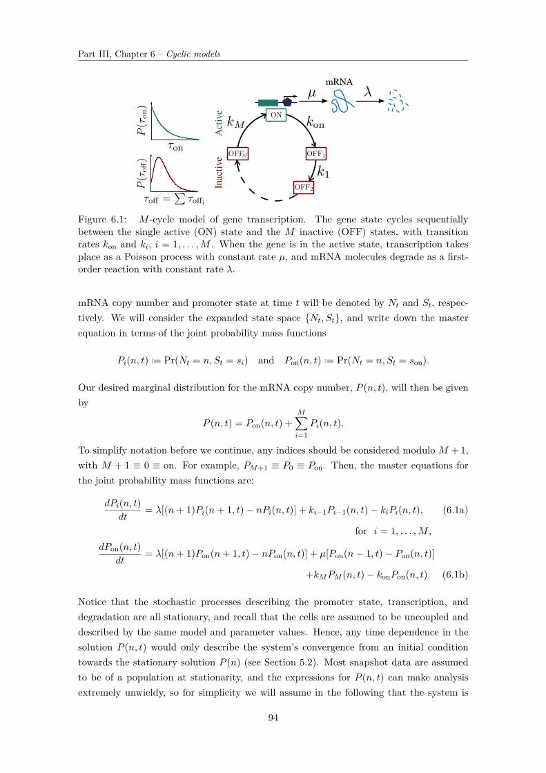
Part III, Chapter 6 – Cyclic models
Active
Inactive
mRNA
Figure 6.1: M -cycle model of gene transcription. The gene state cycles sequentiallybetween the single active (ON) state and the M inactive (OFF) states, with transitionrates kon and ki, i = 1, . . . ,M . When the gene is in the active state, transcription takesplace as a Poisson process with constant rate µ, and mRNA molecules degrade as a first-order reaction with constant rate λ.
mRNA copy number and promoter state at time t will be denoted by Nt and St, respec-tively. We will consider the expanded state space Nt, St, and write down the masterequation in terms of the joint probability mass functions
Pi(n, t) ..= Pr(Nt = n, St = si) and Pon(n, t) ..= Pr(Nt = n, St = son).
Our desired marginal distribution for the mRNA copy number, P (n, t), will then be givenby
P (n, t) = Pon(n, t) +M∑i=1
Pi(n, t).
To simplify notation before we continue, any indices should be considered modulo M + 1,with M + 1 ≡ 0 ≡ on. For example, PM+1 ≡ P0 ≡ Pon. Then, the master equations forthe joint probability mass functions are:
dPi(n, t)dt
= λ[(n+ 1)Pi(n+ 1, t)− nPi(n, t)] + ki−1Pi−1(n, t)− kiPi(n, t), (6.1a)
for i = 1, . . . ,M ,dPon(n, t)
dt= λ[(n+ 1)Pon(n+ 1, t)− nPon(n, t)] + µ[Pon(n− 1, t)− Pon(n, t)]
+kMPM (n, t)− konPon(n, t). (6.1b)
Notice that the stochastic processes describing the promoter state, transcription, anddegradation are all stationary, and recall that the cells are assumed to be uncoupled anddescribed by the same model and parameter values. Hence, any time dependence in thesolution P (n, t) would only describe the system’s convergence from an initial conditiontowards the stationary solution P (n) (see Section 5.2). Most snapshot data are assumedto be of a population at stationarity, and the expressions for P (n, t) can make analysisextremely unwieldy, so for simplicity we will assume in the following that the system is
94

6.2. Solution for P (n) via the probability generating function
already at stationarity and will omit the variable t.
6.2 Solution for P (n) via the probability generating function
In this section we will follow the usual route for solving a system of master equationsof the form (6.1), by transforming them into a system of ordinary differential equationsfor the corresponding probability generating functions. A solution for this model hasbeen published using this method, but the derivation is opaque in parts and the finalexpression is not given explicitly in terms of the parameters of the using a relevant adjugatematrix to show that P (n) can be expressed concisely in terms of gamma functions andhypergeometric functions. The relevant parameter set is the model parameters themselves,and the eigenvalues of the transition matrix for the promoter cycle. As a result, propertiesof the solution, including expressions for the moments and noise, are transparent.
We will use this expression for P (n) to show how the noise characteristics can betuned with the timescales at the promoter, and perform maximum likelihood estimation(MLE) and model selection using the Akaike Information Criterion (AIC) on in silicogenerated data. In doing so, we exemplify how the assumption of the minimal two-state(random telegraph) model can lead to gross mis-estimation of the underlying parameters,and demonstrate that for many parameter regimes snapshot population data cannot beused to infer the underlying timescales. This quantitative data analysis is only possibledue to our possession of the algebraic expression for P (n) that we derive in the nextsubsection.
6.2.1 Derivation of the solution
Define for each state si, i = 1, . . . ,M, on, the stationary probability generating functions
Gi(z) ..=∞∑n=0
znPi(n), Gon(z) ..=∞∑n=0
znPon(n),
and
G(z) ..=∞∑n=0
znP (n) = Gon(z) +M∑i=1
Gi(z).
Transform the master equations (6.1) in the usual manner, by multiplying through by zn
and summing over n ∈ N to obtain, at stationarity:
λ(z − 1)dGidz
= ki−1Gi−1(z, t)− kiGi(z, t), i = 1, . . . ,M, (6.2a)
λ(z − 1)dGondz
= kMGM (z, t)− konGon(z) + µ(z − 1)Gon(z). (6.2b)
Without loss of generality let λ = 1, and to simplify notation, make the change of variable
s ..= µ(z − 1); Hi(s) ..= Gi(z), i = 1, . . . ,M, on,
95

Part III, Chapter 6 – Cyclic models
and write Eqs (6.2) in the form
s dds + k1 −kon
−k1 s dds + k2
−k2. . .. . . s dds + kM
−kM s dds + kon
H1
H2...
HM
Hon
=
00
. . .0
s
H1
H2...
HM
Hon
(6.3)
i.e.(θI −K) H = s eM+1eTM+1 H, (6.4)
where
θ ..= sd
ds, H ..=
H1...
HM
Hon
, eM+1..=
0...01
and K is the state transition matrix
K ..=
−k1 kon
k1 −k2
k2. . .. . . −kM
kM −kon
Before we continue, let us take a small detour to consider some properties of the promoterstate transition matrix K; our desired distribution P (n) ≡ Pr(Nt = n) is a marginal ofthe joint distribution Pr(Nt = n, St = si), so integral conditions based on the propertiesof the continuous-time Markov process Stt≥0, with associated transition rate matrix K,will be required later.
Denote the probability of being in state si at time t by PS (si, t) ..= Pr(St = si), anddefine
PS (s, t) ..=
PS (s1, t)
...PS (sM , t)PS (son, t)
.
By definition of the Markov chain Stt≥0, we have
dPS
dt= K PS .
K clearly has a zero eigenvalue1, and by Gershgorin’s circle theorem (Horn and Johnson
1The columns of K sum to zero, for example.
96

6.2. Solution for P (n) via the probability generating function
1999) the non-zero eigenvalues of K have negative real parts. Hence a stationary solutionπ = (π1, . . . , πM , πon)T always exists, that satisfies
Kπ = 0 ;M+1∑i=1
πi = 1.
π is the eigenvector corresponding to the zero eigenvalue of K, which is normalized sothat its elements sum to 1 (since π represents a probability mass function). It can easilybe shown that π has elements
πi =∏j 6=i kj∑M+1
r=1∏j 6=r kj
.
For example for M = 2, πon = π3 = k1k2/(k2kon + k1kon + k1k2).Returning to the derivation of P (n), sum the rows of Eq. (6.3) to see that
dH
ds≡ d
ds(H1 + · · ·+HM +Hon) = Hon(s), (6.5)
so to determine H(s) ≡ G(z) we need only determine Hon, and integrate once under thecondition H(0) = G(1) = ∑
n P (n) = 1.In order to obtain an uncoupled equation for Hon, we will employ a trick using an
adjugate matrix and capitalise on the structure of the model. Multiply both sides ofEq. (6.4) on the left by the transposed matrix of cofactors adj(θI−K), remembering thatfor any square invertible matrix A, adj(A)A = det(A)I:
det(θI −K) H = adj(θI −K) s eM+1 eTM+1 H (6.6)
=
(−1)M+2MM+1,1
...(−1)2M+2MM+1,M+1
sHon,
where Mi,j is the (i, j)th minor of [θI −K].Notice that the submatrix of [θI−K] formed by deleting the last row and last column
is lower triangular, so
(−1)2M+2MM+1,M+1 = MM+1,M+1 =M∏i=1
(θ + ki).
Also, the determinant is equal to the product of the eigenvalues and hence
det(θI −K) =M+1∏i=1
(θ − νi) = θM∏i=1
(θ − νi),
where the νi are the eigenvalues of the matrix K, and without loss of generality we havetaken νM+1 to be the zero eigenvalue. The first coordinate of this equation is now an
97

Part III, Chapter 6 – Cyclic models
uncoupled equation in terms of Hon only:
θM∏i=1
(θ − νi)Hon(s) =M∏i=1
(θ + ki) sHon(s)
= sM∏i=1
(θ + ki + 1)Hon(s),
where we used the operator identity (θ + a)s = s(θ + a + 1), for a a constant. Thisdifferential equation is satisfied by the generalized hypergeometric function FM M (Erdelyi1953), where
Fp q
[a1, a2 . . . , ap
b1, b2 . . . , bq; z
]..=
∞∑n=0
(a1)n(a2)n . . . (ap)n(b1)n(b2)n . . . (bq)n
zn
n! ,
where (x)n ..= x(x+ 1) . . . (x+ n− 1) = Γ(x+ n)/Γ(x) is Pochhammer’s function2. Thuswe can immediately write down the general solution for Hon:
Hon(s) = c0 FM M
[1 + k1, . . . , 1 + kM1− ν1, . . . , 1− νM
; s]
+M∑i=1
ci sνi FM M
[1 + k1 + νi, . . . . . . , 1 + kM + νi
1 + νi, 1− ν1 + νi, . . ∨ . . , 1− νM + νi; s
], (6.7)
where . . ∨ . . denotes suppression of the term 1− νi + νi, and c0, . . . , cM are constants tobe determined.
Notice that νi ∈ C, and we want sνi ∈ R ∀ s ∈ R. Hence ci = 0 for i = 1, . . . ,M . Weare left only with c0, which is given by:
c0 = Hon(0) ≡ Gon(1) = πon =∏Mj=1 kj∑M+1
r=1∏j 6=r kj
.
Hence Eq. (6.7) is reduced to
Hon(s) = πon FM M
[k1 + 1, . . . , kM + 1−ν1 + 1, . . . , −νM + 1
; s]
=.. πon FM M
[(k) + 1
(−ν) + 1; s
],
where here we have introduced the notation in the latter equation, similar to that usedin (Slater 1966), for compactness and clarity.
2The notation (x)n itself is known as Pochhammer’s symbol. Confusingly, in combinatorics and statis-tics Pochhammer’s function is usually denoted x(n) and is referred to as the rising factorial, whereasPochhammer’s symbol (x)n denotes the falling factorial. However, in the theory of special functionsand in particular the hypergeometric functions that we will be using, Pochhammer’s symbol is standardnotation for Pochhammer’s function, or the rising factorial, as defined in the text.
98

6.2. Solution for P (n) via the probability generating function
Now, recall from Eq. (6.5) that we can integrateHon(s) to obtainH(s). Using standardproperties of generalized hypergeometric functions (Erdelyi 1953), we get
H(s) = πon
∏Mj=1(−νj)∏Mj=1 kj
FM M
[(k)
(−ν); s
]+ cH ,
where cH is a constant of integration. To see that cH = 0, we can use our expression forHon and Eq. (6.3) to obtain HM , . . . ,H1 via back substitution. Since these operations willonly involve differentiation, no function Hi, i = 1, . . . ,M , will have any additive constantterms. Therefore, neither will H ..= H1 + · · ·+HM +Hon, so we must have cH = 0.
Furthermore, we need 1 = ∑n P (n) = G(1) = H(0)†, so we are left with
H(s) = FM M
[(k)
(−ν); s
], or
G(z) = FM M
[(k)
(−ν); µ(z − 1)
]. (6.8)
Now expand G(z) in a Taylor expansion around z = 0 so that we will be able to find P (n)by reading off the coefficient of zn:
G(z) =∞∑n=0
zn
n!dnG
dzn
∣∣∣∣∣z=0
=∞∑n=0
zn
n! µn (k1)n . . . (kM )n
(−ν1)n . . . (−νM )nFM M
[(k) + n
(−ν) + n; −µ
].
Again using some notation introduced in (Slater 1966) for compactness:
Γ[(k) + n, (−ν)
(k), (−ν + n)
]..= Γ(k1 + n)
Γ(k1) . . .Γ(kM + n)
Γ(kM )Γ(−ν1)
Γ(−ν1 + n) . . .Γ(−νM )
Γ(−νM ) + n,
we finally have
P (n) = (k1)n . . . (kM )n(−ν1)n . . . (−νM )n
µn
n! FM M
[(k) + n
(−ν) + n; −µ
]
†Incidentally, this property provides us with an expression for the pseudo-inverse of the promoter statetransition matrix K:
1 = H(0) =∏M
j=1(−νj)∏M
j=1 kjπon =
∏M
j=1(−νj)∏M
j=1 kj
∏M
j=1 kj∑M+1r=1
∏j 6=r kj
,
i.e.M+1∑r=1
∏j 6=r
kj =M∏j=1
(−νj) = (−1)M × pseudo-inverse of K.
99

Part III, Chapter 6 – Cyclic models
= Γ[(k) + n, (−ν)
(k), (−ν + n)
]µn
n! FM M
[(k) + n
(−ν) + n; −µ
]. (6.9)
Example 6.2–1 — Rederivation of the solution of the random telegraphmodel (1-cycle)
It is easy to check that our results reproduce the known solution of the random tele-graph model (Ko 1991; Peccoud and Ycart 1995; Raj et al. 2006; Iyer-Biswas et al.2009). Substituting M = 1 into the above, we have
K =(−k1 kon
k1 −kon
), (6.10)
with eigenvalues ν1 = −(kon + k1) and ν2 = 0. Eq. (6.9) then becomes
P (n) = Γ(k1 + n)Γ(k1)
Γ(kon + k1)Γ(kon + k1 + n)
µn
n! F1 1 (k1 + n, kon + k1 + n;−µ) , (6.11)
as shown in (Raj et al. 2006; Iyer-Biswas et al. 2009).
Example 6.2–2 — Explicit solution for the 2-cycle
The 2-cycle has already been proposed to account for the non-exponential waitingtimes observed in the inactive gene state in single-molecule, single-cell time coursedata (Suter et al. 2011; Molina et al. 2013; Harper et al. 2011; Kandhavelu et al.2012). However, an algebraic expression for P (n) was not available so fitting andanalysis was done computationally. Using Eq. (6.9) we can straightforwardly write thedown the required expression.
For M = 2, (ν) = ν1, ν2 are the non-zero eigenvalues of K, which are
ν1,2 = 12
(−kon − k1 − k2 ±
√(kon − k1 − k2)2 − 4k1k2
), (6.12)
100

6.2. Solution for P (n) via the probability generating function
so the stationary solution of the model is
P (n) = Γ(k1 + n)Γ(k1)
Γ(k2 + n)Γ(k2)
Γ(−ν1)Γ(−ν1 + n)
Γ(−ν2)Γ(−ν2 + n)
µn
n! F2 2
[k1 + n, k2 + n
−ν1 + n, −ν2 + n; −µ
].
(6.13)
6.2.2 Noise regulation
With the exact solution, and certain other elements of its derivation, we can obtain prop-erties of the M -cycle and analyse how they differ from the two-state random telegraphmodel (the 1-cycle).
First, the moments can be straightforwardly obtained from the probability generatingfunction (Eq. (6.8)):
E (N) = dG
dz
∣∣∣∣∣z=1
= µ
∏Mi=1 ki∏M
i=1(−νi), (6.14)
and
Var(N) = d2G
dz2
∣∣∣∣∣z=1
+ dG
dz
∣∣∣∣∣z=1
−
dGdz
∣∣∣∣∣z=1
2
(6.15)
= µ
∏Mi=1 ki∏M
i=1(−νi)
(µ
∏Mi=1(ki + 1)∏Mi=1(−νi + 1)
+ 1− µ∏Mi=1 ki∏M
i=1(−νi)
). (6.16)
However, it would be helpful to write these expressions explicitly in terms of the expectedwaiting times in each state, denoted
τon = 1kon
, τi = 1ki, and τoff =
M∑i=1
τi.
Thus we need to employ some manoeuvres to obtain expressions for ∏Mi=1(−νi) and∏M
i=1(−νi+1). For the former, we continue from the last footnote remarking thatH(0) = 1implies that:
M∏j=1
(−νj) =M+1∑r=1
∏j 6=r
kj
=M+1∑r=1
1kr
M+1∏i=1
ki
=M+1∑r=1
τr
M+1∏i=1
1τi
= τon + τoff
τon∏Mi=1 τi
. (6.17)
101

Part III, Chapter 6 – Cyclic models
In order to obtain a similar expression for ∏Mi=1(−νi + 1), notice that it is equal to the
determinant of the matrix [I −K] (since νM+1 = 0):
M∏i=1
(−νi + 1) =M+1∏i=1
(−νi + 1) (6.18)
= det(I −K)
= det
1 + k1 −kon
−k1 1 + k2
−k2. . .. . . 1 + kM
−kM 1 + kon
= (−1)M+2(−kon)(−k1) . . . (−kM ) + (−1)2M+2(1 + kon)(1 + k1) . . . (1 + kM )
= (1 + kon)M∏i=1
(1 + ki)− kon
M∏i=1
ki
= (τon + 1)∏Mi=1(τi + 1)− 1
τon∏Mi=1 τi
. (6.19)
Substituting these expressions in terms of waiting times (Eqs (6.17) and (6.19)) into theexpressions for the mean and variance obtained above (Eqs (6.14) and (6.15)), we have
E (N) = µ∏Mi=1 ki
(τon + τoff)kon∏Mi=1 ki
(6.20)
= µ τonτon + τoff
,
Var(N) = E (N)(
µ τon∏Mi=1(τi + 1)
(τon + 1)∏Mi=1(τi + 1)− 1
+ 1− E (N)). (6.21)
Notice that the expression for E (N) is the same as for the random telegraph model; it isthe expectation for the constitutive (Poisson) model with only one state, µ, scaled by theproportion of time the promoter is active. In particular, the expectation is independentof the individual expected waiting times τi in each inactive state, although the variance isnot. Hence we may fix the waiting times τon and τoff = ∑
τi, thus fixing the expectation,whilst tuning the noise by varying the expected waiting time in each inactive state τi.
Let us investigate in more detail how noise is affected by the choice of τi, i = 1, . . . ,M ,and byM , the number of inactive states. We will use the ensemble Fano factor as a measurefor noise, although we would arrive at the same conclusions if we chose the coefficient ofvariation, η ..=
√Var(N)/E (N) instead, since we have fixed E (N) = τon/(τon +τoff). Since
the number of inactive states will now be a variable, we will specify it using a superscript,
102
6.2. Solution for P (n) via the probability generating function
i.e., Fano(2) refers to the Fano factor for the 2-cycle. The waiting times τi are also variables,but it should not cause confusion if we do not specify them explicitly.
Suppose τon and τoff are fixed constants, but the τi, i = 1, . . . ,M , can vary under theconstraints
τi > 0, i = 1, . . . ,M, andM∑i=1
τi = τoff .
For now, the number of inactive states M is fixed. Using Eqs (6.20) and (6.21), we have
Fano(M) ..= Var(N)E (N)
= µ τon∏Mi=1(τi + 1)
(τon + 1)∏Mi=1(τi + 1)− 1
+ 1− E (N) ,
which we can minimize over the τi’s using for example the method of Lagrange multipliers.The minimum Fano(M)
min occurs when τi = τj = τoff/M ∀ i, j ∈ 1, . . . ,M, giving
Fano(M) ≥ Fano(M)min = µ τon(τoff/M + 1)M
(τon + 1)(τoff/M + 1)M − 1 + 1− E (N) .
On the other hand, the maximum possible Fano factor occurs at the other extreme ofτi-space, where without loss of generality τ1 → τoff , and τi → 0, i = 2, . . . ,M . Notice thatin the limit τi = 0, i = 2, . . . ,M , the M -cycle is reduced to the 1-cycle, i.e. the usualtwo-state random telegraph model, so we have:
Fano(M) ≤ Fano(M)max < Fano(1)
= µ τon(τoff + 1)(τon + 1)(τoff + 1)− 1 + 1− E (N)
= µ τonτ2off
(τonτoff + τon + τoff)(τon + τoff) + 1.
Now to see how the number of states M affects the noise characteristics of the model,we now allow M to be a variable. Consider first the expression above for Fano(M)
min , theminimum Fano factor given M . The function
g(M) ..= µτon(τoff/M + 1)M(τon + 1)(τoff/M + 1)M − 1 ,M ∈ N
is a monotonically decreasing function of M , hence (since E (N) is fixed) the minimumpossible Fano factor for anM -cycle decreases as the number of inactive statesM increases:
Fano(L)min < Fano(M)
min ∀ L > M.
Since any M -cycle reduces to the 1-cycle in the limit τ1 = τoff , τi = 0, i = 2, . . . ,M , wehave
sup(Fano(M)
max
)= Fano(1).
103

Part III, Chapter 6 – Cyclic models
To sum up, for an M -cycle model with expected waiting times in the inactive states τi,i = 1, . . . ,M , the Fano factor Fano(M) satisfies
Fano(L)min < Fano(M)
min ≤ Fano(M) < Fano(1)min ≡ Fano(1)
max ≡ Fano(1) ∀ L > M > 1.
In other words, assuming the simple two-state random telegraph model of gene tran-scription necessarily implies assuming the maximum level of noise for the given expectedwaiting times. It is well-known that negative feedback motifs can reduce gene expres-sion noise (Austin et al. 2006; Nevozhay et al. 2009; Shimoga et al. 2013), but here wehave shown that we may achieve similar effects via the introduction of additional genestates, and/or tuning the transition rates towards the parameter regime τi = τoff/M, i =1, . . . ,M .
6.3 Estimating parameter values and model selection
In 2006 Raj et al. published their seminal paper where for the first time the exact expres-sion for P (n) for the 1-cycle (random telegraph model) was known, and could be used tofit to their fluorescence in situ hybridization (FISH) data (Raj et al. 2006). More recently,several different 1-cycle parameter regimes have been shown to fit snapshot data for yeastequally well (Zenklusen et al. 2008; Senecal et al. 2014), and several groups have shown thatwaiting time distributions in the inactive state are not exponentially distributed (whichthe 1-cycle can not account for) (Suter et al. 2011; Zoller et al. 2015; Harper et al. 2011).Nevertheless, in the absence of an exact, practical3 solution, it remains common practiceto estimate transcription rates and timescales at the promoter by fitting snapshot datato the solution of the 1-cycle, or by using expected waiting times τon and τoff to estimatethe 1-cycle transition rates kon = 1/τoff and koff = 1/τon (Suter et al. 2011; Senecal et al.2014).
Now that we have the exact solution explicitly in terms of measurable parameters, wecan use it to estimate M -cycle parameter values for snapshot data, and perform quanti-tative model selection. As an example, we generated in-silico snapshot data for 5-cyclemodels designed to mimic the results published in (Zoller et al. 2015), where M -cyclesare fitted to time-lapse data. We then used maximum likelihood estimation (MLE) toestimate the parameter values under the assumptions of several M -cycle models, and theAkaike Information Criterion (AIC) to perform model selection. We use these results:
• to exemplify how the assumption of the minimal 1-cycle (random telegraph) modelcan lead to gross mis-estimation of the underlying parameters; and
• to demonstrate that for many parameter regimes, snapshot population data cannotbe used to infer the underlying timescales. In those cases single-cell time seriesanalysis is necessary to validate the results.
3Although an exact solution for theM -cycle was published in 2012 (Zhang et al. 2012), it was not givenexplicitly in terms of the model parameters µ, k1, . . . , kM , kon as we were able to do here.
104

6.3. Estimating parameter values and model selection
However, a thorough parameter fitting exercise would require more detailed investiga-tions into which measures should be used to measure disparity between two probabilitydistributions.
6.3.1 Generating in-silico data
To be able to critically analyse the output of the MLE, we generated several sets of in-silicodata using Gillespie’s stochastic simulation algorithm (SSA) (Gillespie 1977). The expres-sion for P (n) (Eq. (6.9)) was derived under assumptions that imply an ergodic system, soto obtain “snapshot” data it is sufficient to simulate a single time trace η(t)0≤t≤T forthe number of mRNA transcripts in a single cell4. We conservatively discarded the first1000 minutes after the sample path first reached its expected mean value to avoid effectsfrom the initial condition. Then, what we refer to as the empirical probability distributionPemp was given by
Pemp(n) = 1T
∫ T
01n(η(t))dt,
where 1n is the indicator function:
1n(η(t)) =
1 if η(t) = n,
0 otherwise.
We sampled 200 data points from the empirical distribution to use in the maximum like-lihood estimation procedure.
To work only within biologically relevant parameter regimes, we used the models andparameter values for the NcKap1 and Hmga2 genes, which were recently estimated fromtime-lapse recordings of mammalian cells (Zoller et al. 2015).
6.3.2 Maximum Likelihood estimation and model selection
Despite the expression for P (n) (6.9) being a concise function of relatively few parame-ter combinations, the gamma functions and generalized hypergeometric function lead tounwieldy likelihood and log-likelihood functions that are impractical to maximise analyt-ically. As such, we used the ‘Squeeze-and-breathe’ numerical optimization algorithm tomaximise the log-likelihood function, since it has been shown to be robust to situationswhere parameter values may span several orders of magnitude, and can find parameterregimes that lie outside of the range of the initial prior (Beguerisse-Díaz et al. 2012). Themethod iteratively refines a sequence of parameter distributions using local optimisationand partial resampling of the historical prior, followed by ranking and culling of the lo-cal optima. The iteration continues until the parameter distributions and the negativelog-likelihood values converge.
The results of the parameter estimation process for the NcKap1 and Hmga2 genes4As per the discussions in Sections 4.2.2 and Example 5.1–1, an estimate for P (n) could have been
obtained quicker using sample paths of X instead of N . However, the simulation process here was notprohibitively slow because only one sample path was required.
105
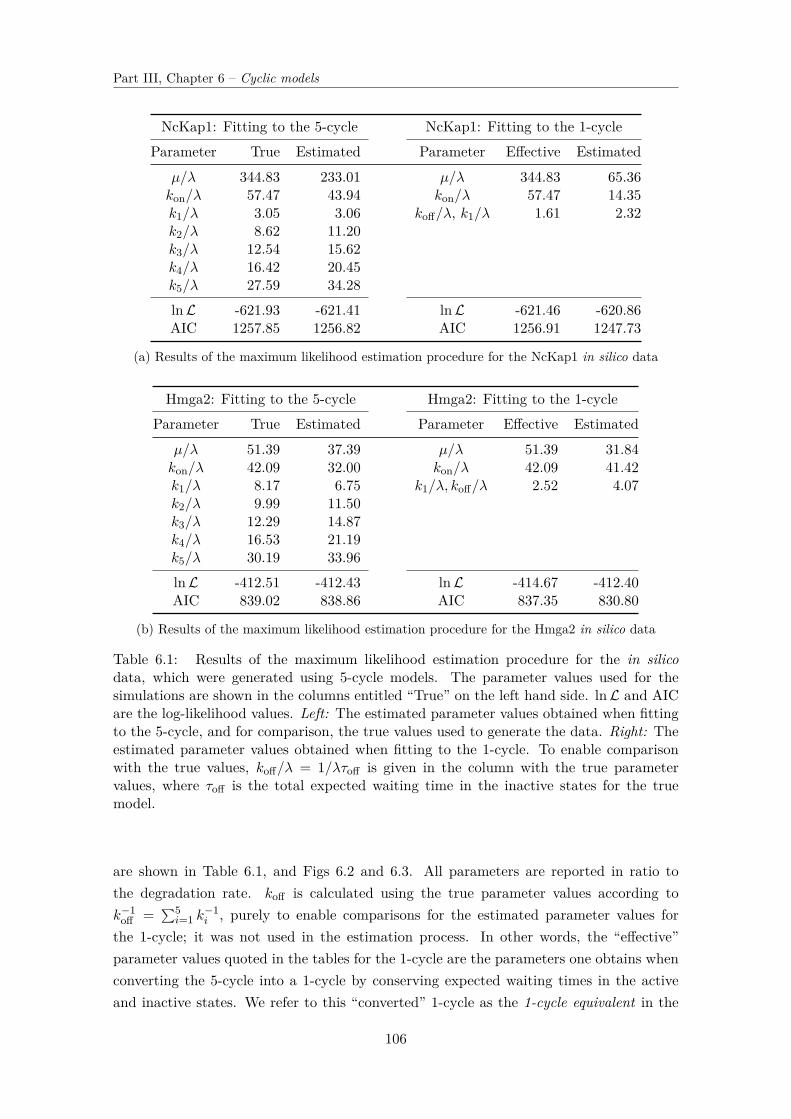
Part III, Chapter 6 – Cyclic models
NcKap1: Fitting to the 5-cycle NcKap1: Fitting to the 1-cycleParameter True Estimated Parameter Effective Estimated
µ/λ 344.83 233.01 µ/λ 344.83 65.36kon/λ 57.47 43.94 kon/λ 57.47 14.35k1/λ 3.05 3.06 koff/λ, k1/λ 1.61 2.32k2/λ 8.62 11.20k3/λ 12.54 15.62k4/λ 16.42 20.45k5/λ 27.59 34.28lnL -621.93 -621.41 lnL -621.46 -620.86AIC 1257.85 1256.82 AIC 1256.91 1247.73
(a) Results of the maximum likelihood estimation procedure for the NcKap1 in silico data
Hmga2: Fitting to the 5-cycle Hmga2: Fitting to the 1-cycleParameter True Estimated Parameter Effective Estimated
µ/λ 51.39 37.39 µ/λ 51.39 31.84kon/λ 42.09 32.00 kon/λ 42.09 41.42k1/λ 8.17 6.75 k1/λ, koff/λ 2.52 4.07k2/λ 9.99 11.50k3/λ 12.29 14.87k4/λ 16.53 21.19k5/λ 30.19 33.96lnL -412.51 -412.43 lnL -414.67 -412.40AIC 839.02 838.86 AIC 837.35 830.80
(b) Results of the maximum likelihood estimation procedure for the Hmga2 in silico data
Table 6.1: Results of the maximum likelihood estimation procedure for the in silicodata, which were generated using 5-cycle models. The parameter values used for thesimulations are shown in the columns entitled “True” on the left hand side. lnL and AICare the log-likelihood values. Left: The estimated parameter values obtained when fittingto the 5-cycle, and for comparison, the true values used to generate the data. Right: Theestimated parameter values obtained when fitting to the 1-cycle. To enable comparisonwith the true values, koff/λ = 1/λτoff is given in the column with the true parametervalues, where τoff is the total expected waiting time in the inactive states for the truemodel.
are shown in Table 6.1, and Figs 6.2 and 6.3. All parameters are reported in ratio tothe degradation rate. koff is calculated using the true parameter values according tok−1
off = ∑5i=1 k
−1i , purely to enable comparisons for the estimated parameter values for
the 1-cycle; it was not used in the estimation process. In other words, the “effective”parameter values quoted in the tables for the 1-cycle are the parameters one obtains whenconverting the 5-cycle into a 1-cycle by conserving expected waiting times in the activeand inactive states. We refer to this “converted” 1-cycle as the 1-cycle equivalent in the
106

6.3. Estimating parameter values and model selection
figures showing probability mass functions (pmfs) and cumulative mass functions (cmfs)for the 1-cycles (bottom rows), again solely for the purposes of comparison.
Using the log-likelihood values, we can use the AIC to select the preferred model for thedata we used. The AIC is a measure for statistical model selection based on informationtheory (Akaike 1974), defined by
AIC ..= −2 lnL+ 2(number of independently adjusted parameters within the model).
The AIC values are shown in Tables 6.1; the preferred model is the one with lowest AICvalue.
n
0 10 20 30 40
P(n
)
0
0.02
0.04
0.06
0.08NcKap1 5-cycle pmfs
EmpiricalMLETheoretical
n
0 10 20 30 40
F(n
)
0.0
0.2
0.4
0.6
0.8
1.0NcKap1 5-cycle cmfs
n
0 10 20 30 40
P(n
)
0
0.02
0.04
0.06
0.08NcKap1 1-cycle pmfs
EmpiricalMLETheoreticalTheoretical
1-cycle equivalent
n
0 10 20 30 40
F(n
)
0.0
0.2
0.4
0.6
0.8
1.0NcKap1 1-cycle cmfs
Figure 6.2: The probability mass functions P (n) and cumulative mass functions F (n) forthe NcKap1 empirical data (blue) and the theoretical mass functions, calculated using: theparameter values from the maximum likelihood estimation (red); true parameter values(yellow); and the parameter values for the 1-cycle with the same expected waiting timesin each gene state as the true model (purple). The legends apply to both the pmf and cmfgraphs.
There are several observations to be made from these maximum likelihood estimatesand corresponding AIC values. First, the 1-cycle maximum likelihood parameter estimatesdo better in terms of the log-likelihood lnL than both the true values, and the estimatesobtained when fitting the 5-cycle (the true model). Second, since the log-likelihood valuesfor the fitted models are very similar, selection using the AIC amounts to choosing themodel with the fewest parameters, in this case the 1-cycle. However, the 1-cycle parametervalues are grossly mis-estimated. Although the 5-cycle estimates are incorrect, they aresignificantly closer to the true values than the 1-cycle estimates are, in particular for µ/λ.
Third, as can be clearly seen from the figures, we recover the observations from Zen-
107

Part III, Chapter 6 – Cyclic models
n
0 5 10 15
P(n
)
0.00
0.05
0.10
0.15
0.20
0.25Hgma2 5-cycle pmfs
EmpiricalMLETheoretical
n
0 5 10 15
F(n
)
0.0
0.2
0.4
0.6
0.8
1.0Hgma2 5-cycle cmfs
n
0 5 10 15
P(n
)
0.00
0.05
0.10
0.15
0.20
0.25Hgma2 1-cycle pmfs
EmpiricalMLETheoreticalTheoretical
1-cycle equivalent
n
0 5 10 15
F(n
)0.0
0.2
0.4
0.6
0.8
1.0Hgma2 1-cycle cmfs
Figure 6.3: The probability mass functions P (n) and cumulative mass functions F (n) forthe Hmga2 empirical data (blue) and the theoretical mass functions, calculated using: theparameter values from the maximum likelihood estimation (red); true parameter values(yellow); and the parameter values for the 1-cycle with the same expected waiting timesin each gene state as the true model (purple). The legends apply to both the pmf and cmfgraphs.
klusen et al. 2008 that these models are unidentifiable – several different models can fitpopulation snapshot data equally well. The estimated parameter values outperform thetrue parameter values when maximising the log-likelihood function, suggesting that thelog likelihood function is extremely flat for these models, and perhaps not an effectivemeasure for these models. Precision tolerances must be kept low when maximising thelog-likelihood function numerically, and one typically needs to restrain the parameter spaceif possible (Murphy and Vaart 2000).
Taken together, these results issue a stark warning to those inferring timescales ofactivities at the promoter from snapshot data (Raj et al. 2006; Taniguchi et al. 2010;Senecal et al. 2014; Bahar Halpern et al. 2015), even with more complex models than thesimple 1-cycle. In particular, good fits to the empirical distribution are not necessarilyindicative of the best parameter estimates; the 1-cycle equivalent effective parametersproduce the worst fits to the data (Figs 6.2 and 6.3), but the timescales implied by themare closer to reality than those implied by the MLE for the 1-cycle.
There are several functions apart from the likelihood or log-likelihood that can be usedto measure the disparity between two discrete probability distributions, for example theKullback-Leibler divergence or the related Jensen-Shannon divergence, the total variationdistance, or the Wasserstein (or earth mover’s) distance, to name just a few. Each diver-gence or metric has a bias towards certain kinds of differences between two distributions,
108

6.4. Solution for fX
for example the Kullback-Leibler divergence emphasizes tails more strongly than the totalvariation distance. A thorough parameter-fitting exercise would need to check the resultsobtained from several appropriate divergences or metrics, possibly defining a new measureif a particular property of the distribution needed to be given particular importance. Vali-dation using single-cell time series analysis is in general necessary to confirm the reliabilityof the results (Zoller et al. 2015; Suter et al. 2011).
6.4 Solution for fX
Recall from Chapter 3 that the probability mass function P (n) for the mRNA copy numbercan be written in Poisson mixture form
P (n) =∫ξn e−ξ
n! fX(ξ) dξ,
so that one route to obtaining P (n) is simply to search for the mixing density fX . Sincewe already have an explicit expression for P (n) from the previous section, we will not needto use the Poisson mixture property to obtain a solution of the M -cycle. However, thevalue of fX extends far beyond simply being a stepping stone towards an expression forP (n). Since fX is the central, model-specific core of any transcription-degradation model,we gain a deeper understanding of the mathematical structure and properties of the modelthan we do when only looking at P (n). After deriving fX using the multistate Kramers-Moyal equations, in Section 6.4.2 we will use it to help navigate parameter space to searchfor qualitatively different solution behaviours. We defer discussion of the mathematicalstructures that reveal themselves when deriving fX until Chapter 7, as the scope extendsbeyond M -cycle models.
6.4.1 Derivation of the solution
The M -cycle is a multistate promoter model that falls within the framework described inSection 4.4 on the multistate Kramers-Moyal equations: we have a Markov jump processS between M + 1 discrete states s1, . . . , sM , son, and the bivariate process X,S isMarkovian. Therefore we can straightforwardly write down the multistate Kramers-Moyalequations in the same way as we did for the solution of the leaky random telegraph model(Example 4.4–1).
Define for each state s1, . . . , sM , son the joint probability density function fi(x) ..=fX,S(x, si), and recall the convention introduced in Section 6.1 that indices should beconsidered modulo M + 1, with M + 1 ≡ 0 ≡ on. The law of total probability gives us
fX(x) =M+1∑i=1
fi(x),
109
Part III, Chapter 6 – Cyclic models
and the multistate Kramers-Moyal equations are (Pawula 1967; Pawula 1970):
d
dx[−λxfi(x)] = ki−1fX,S(x, si−1)− kifi(x), i = 1, . . . ,M, and (6.22a)
d
dx[(µ− λx)fon(x)] = kMfM (x)− konfon(x). (6.22b)
To simplify notation, set λ = 1 and use the change of variables z = λx/µ. We will keep thesame notation for the joint probability density functions, but specify the variable for themarginal, i.e. we will now work to obtain fZ(z) = f1(z) + · · ·+ fM (z) + fon(z)z ∈ (0, 1).Eqs (6.22) become
d
dz[A(z)f(z)] = Kf(z), (6.23)
where f = (f1, . . . , fM , fon)T , A(z) = (eM+1eTM+1 − zI), eM+1 = (0, . . . , 0, 1)T , and K isthe state transition matrix
K =
−k1 kon
k1 −k2
k2. . .. . . −kM
kM −kon
As we saw in Section 6.2.1, K has a zero eigenvalue and by Gershgorin’s circle theoremthe non-zero eigenvalues of K have negative real parts, so a stationary solution exists.The probabilities πi =
∫ 10 fi(z) dz of being in state si, i = 1, . . . , sM , son, evolve to an
equilibrium state given by the eigenvector π that corresponds to the zero eigenvalue,where
πi =∫ 1
0fi(z) dz =
∏j 6=i kj∑M+1
r=1∏j 6=r kj
. (6.24)
Now, integrating (6.23) we have
[A(z)f(z)]10 = K
∫ 1
0f(z) dz = Kπ = 0,
hence we get the boundary conditions
fi(1) = 0, i = 1, . . . ,M, and (6.25a)
fon(0) = 0. (6.25b)
Also, for 1T := (1, . . . , 1), we have
ddz(1TA(z)f
)= 1TKf = 0
110
6.4. Solution for fX
(equivalent to summing the rows), so that
1TA(z)f = −zf1(z)− · · · − zfM (z) + (1− z)fon(z) = C. (6.26)
Equation (6.26) is true for all z ∈ (0, 1), so substituting in z = 0 or z = 1 we can showthat the constant of integration C is equal to 0. Hence
fZ =M+1∑i=1
fi = 1zfon, (6.27)
so we need only solve the Kramers-Moyal equations (6.23) for fon, the marginal probabilitydensity corresponding to the active state. In order to obtain an uncoupled equation forfon, we will employ the same trick we used in Section 6.2.1, using an adjugate matrix andcapitalise on the structure of Eq. (6.23).
Define θ ..= z ddz and write the Kramers-Moyal equations (6.23) in the form
(θI + I +K) f = eM+1eTM+1
1zθ f .
Multiply both sides on the left by the transposed matrix of cofactors adj(θI + I + K),remembering that for any square invertible matrix A, adj(A)A = det(A)I:
det(θI + I +K) f = adj(θI + I +K) eM+1eTM+1
1zθf
=
(−1)M+2MM+1,1
...(−1)2M+2MM+1,M+1
1zθ fon,
where Mi,j is the (i, j)th minor of [θI + I +K].
Notice that the submatrix of [θI + I + K] formed by deleting the M th row and theM th column is lower triangular, so
MM+1,M+1 =M∏i=1
(θ + 1− ki).
Also, the determinant is equal to the product of the eigenvalues and hence
det(θI + I +K) =M+1∏i=1
(θ + 1 + νi),
where the νi are the eigenvalues of the matrix K. The M th coordinate of this equation isnow an uncoupled equation in terms of fon only:
M+1∏i=1
(θ + 1 + νi) fon(z) =M∏i=1
(θ + 1− ki)1zθ fon(z)
111

Part III, Chapter 6 – Cyclic models
= 1z
M∏i=1
(θ − ki) θ fon(z), (6.28)
where we used the operator identity (θ+ a)1z = 1
z (θ+ a− 1). This is a Fuchsian5 equationof order M + 1 with singularities at 0, 1, and +∞, so we can write down the solutionof this equation directly in terms of generalised hypergeometric functions (Slater 1966).When the ki are distinct modulo 1, the general solution is given by
fon(z) = c0 z0 FM+1 M
[1 + ν1, . . . . . . , 1 + νM , 11− k1, . . ∨ . . , 1− kM
; z]
+M∑i=1
ci zki FM+1 M
[1 + ν1 + ki, . . . . . . , 1 + νM + ki, 1 + ki
1− k1 + ki, . . ∨ . . , 1− kM + ki, 1 + ki; z
](6.29a)
≡ c0 FM+1 M
[1 + ν1, . . . . . . , 1 + νM , 11− k1, . . ∨ . . , 1− kM
; z]
+M∑i=1
ci zki FM M−1
[1 + ν1 + ki, . . . . . . , 1 + νM + ki
1− k1 + ki, . . ∨ . . , 1− kM + ki; z
], (6.29b)
where without loss of generality we have taken νM+1 to be the zero eigenvalue of K, andc0, . . . , cM are constants. Here . . ∨ . . denotes suppression of the term 1 − ki + ki, and
FM+1 M and FM M−1 are generalised hypergeometric functions (Erdelyi 1953).
At this point, we will adopt the contracted notation introduced in (Slater 1966), asit will greatly improve clarity later on. For generalized hypergeometric functions we willwrite
Fp q
[a1, . . . , ap
b1, . . . , bq; z
]=.. Fp q
[(a)(b)
; z],
for a product of several Gamma functions we will write
Γ(a1)Γ(a2) . . .Γ(ap)Γ(b1)Γ(b2) . . .Γ(bq)
=.. Γ[a1, a2, . . . , ap
b1, b2, . . . , bq
]
=.. Γ[(a)(b)
],
and a dash will denote the omission of a zero factor in a sequence, for example
(a)′ − ai ..= a1 − ai, . . . , ai−1 − ai, ai+1 − ai, . . . , ap − ai.
The general solution (6.29b) can then be written
fon(z) = c0 FM M−1
[1 + (ν)1− (k)′
; z]
+M∑i=1
ci zki FM M−1
[1 + (ν) + ki
1− (k)′ + ki; z
], (6.30)
5Fuchsian equations will be defined and discussed in Chapter 7.
112
6.4. Solution for fX
where (ν) denotes the sequence ν1, . . . , νM (we omit νM+1 = 0), and (k) denotes thesequence k1, . . . , kM .
Now, recall that fZ(z) = fon(z)/z, and the boundary condition (6.25b) implies thatc0 = 0, so finally we have the general solution
fZ(z) =M∑i=1
ci zki−1 FM M−1
[1 + (ν) + ki
1− (k)′ + ki; z
]. (6.31)
The constants ci can be determined using the integral constraints∫ 1
0 fi(z) dz = πi and∫ 10 fZ(z) dz = 1, and the identity (Rainville 1960)
∫ 1
0zk−1 Fp p−1
[(a)(b)
; z]dz = 1
kFp+1 p
[(a), k
(b), k + 1; 1
].
However, using the solution for P (n) derived in Section 6.2.1 and the Poisson mixtureresult, we can do better. First, use our general solution for fZ (6.31) to write down anexpression for P (n) using the Poisson mixture result:
P (n) =∫ 1
0
(µz)nn! e−µz
M∑i=1
ci zki−1 FM M−1
[1 + (ν) + ki
1− (k)′ + ki; z
]dz
= µn
n!
M∑i=1
ci
∫ 1
0e−µz zki−1+n FM M−1
[1 + (ν) + ki
1− (k)′ + ki; z
]dz. (6.32)
Now, identity 4.8.3.13 from (Slater 1966) is (with letters and symbols as found in thereference):
Γ[(a) + s
(c) + s
]FA+E A+F
[(a) + s, (e)(c) + s, (f)
; y]
=A∑µ=1
Γ[(a)− aµ(c)− aµ
] ∫ 1
0xs+aµ−1 FA A−1
[1 + aµ − (c)1 + aµ − (a)′
; x]
FE F
[(e)(f)
; xy]dx,
for E < F or for E = F and |y| < 1. Use this identity with E = F = 0, (e) = (f) = (0),(a) = (k), (c) = (−ν), and y = −µ to write our explicit solution for P (n) (6.9) in the form
P (n) = Γ[(k) + n, (−ν)(k), (−ν) + n
]µn
n! FM M
[(k) + n
(−ν) + n; −µ
]
= µn
n!
M∑i=1
Γ[(−ν)(k)
]Γ[
(k)′ − ki(−ν)− ki
] ∫ 1
0e−µz zki−1+n FM M−1
[1− (−ν) + ki
1− (k)′ + ki; z
]dz.
(6.33)
113

Part III, Chapter 6 – Cyclic models
Finally, compare Eqs (6.32) and (6.33) to find
ci = Γ[(−ν)(k)
]Γ[
(k)′ − ki(−ν)− ki
].
Putting everything together, we finally obtain the solution
fZ(z) = Γ[(−ν)(k)
]M∑i=1
Γ[
(k)′ − ki(−ν)− ki
]zki−1 FM M−1
[1 + (ν) + ki
1− (k)′ + ki; z
], (6.34)
for z ∈ (0, 1). We can easily obtain fX by changing variables back to X = µZ/λ:
fX(x) = λ
µfZ
(λ
µz
)(6.35)
= λ
µΓ[(−ν)(k)
]M∑i=1
Γ[
(k)′ − ki(−ν)− ki
] (λ
µ
)ki−1xki−1 FM M−1
[1 + (ν) + ki
1− (k)′ + ki; λµx
],
(6.36)
for x ∈ (0, µ/λ).
Example 6.4–1 — Rederivation of the solution of the random telegraphmodel (1-cycle)
As for the explicit solution for P (n) (6.9), we can easily check that our results reproducethe known solution of the random telegraph model (Ko 1991; Peccoud and Ycart 1995;Raj et al. 2006; Iyer-Biswas et al. 2009). For M = 1, λ = 1 we have eigenvaluesν1 = −(kon + k1) and ν2 = 0. Eq. (6.34) then becomes
fZ(z) = Γ(kon + k1)Γ(k1)
1Γ(kon + k1 − k1) z
k1−1 F1 0 [1− kon − k1 + k1 ; z ]
= Γ(kon + k1)Γ(k1)Γ(kon) z
k1−1(1− z)kon−1 .
In other words, Z ∼ Beta(k1, kon), so the final solution is a Poisson-Beta mixture:
P (n) =∫ 1
0
(µz)nn! e−µz
Γ(k1 + k2)Γ(k1)Γ(k2) z
k1−1(1− z)k2−1 dz
= Γ (k1 + n)Γ (k1)
Γ (kon + k1)Γ (kon + k1 + n)
µn
Γ (n+ 1) F1 1 (k1 + n, kon + k1 + n;−µ) ,
as shown in (Raj et al. 2006; Iyer-Biswas et al. 2009).
114

6.4. Solution for fX
Example 6.4–2 — Mixture distribution for the 2-cycle
For M = 2, (ν) = ν1, ν2 are the non-zero eigenvalues of K, which are
ν1,2 = 12
(−kon − k1 − k2 ±
√(kon − k1 − k2)2 − 4k1k2
),
so the stationary solution of the mixing density is
fZ(z) = Γ(−ν1)Γ(−ν2)Γ(k1)Γ(k2)
(Γ(k2 − k1) zk1−1
Γ(−ν1 − k1)Γ(−ν2 − k1) F2 1
[1 + ν1 + k1, 1 + ν2 + k1
1− k2 + k1; z
]
+ Γ(k1 − k2) zk2−1
Γ(−ν1 − k2)Γ(−ν2 − k2) F2 1
[1 + ν1 + k2, 1 + ν2 + k2
1− k1 + k2; z
])
= Γ(−ν1)Γ(−ν2)Γ(k1)Γ(k2)
(Γ(k2 − k1) zk1−1(1− z)kon−1
Γ(−ν1 − k1)Γ(−ν2 − k1) F2 1
[−ν1 − k2,−ν2 − k2
1− k2 + k1; z
]
+ Γ(k1 − k2) zk2−1(1− z)kon−1
Γ(−ν1 − k2)Γ(−ν2 − k2) F2 1
[−ν1 − k1,−ν2 − k1
1− k1 + k2; z
]).
6.4.2 Using the mixing density to analyse parameter spaces
We would like to be able to use the exact expression (6.35) for the mixing density todemarcate the parameter space into regions that produce qualitatively different solutionbehaviour for P (n), for example to find bimodality. The usefulness of this technique hasalready been shown for a certain type of feedback model (Iyer-Biswas and Jayaprakash2014).
For example, Zhang et al. 2012 searched for multimodality in the solution P (n) of the2-cycle via large-scale sampling of the system parameters; with our possession of fZ wecan deduce that multimodality does not exist6 for any M -cycle: Recall from Eq. (6.28)that fon is Fuchsian with only 2 finite singularities, and therefore so are fZ and fX . SinceP (n) = E(Xne−X/n!), P (n) can be bimodal, but not multimodal (see Chapter 7 for amore detailed discussion about what we can learn from the Fuchsian properties).
To see if we can deduce any more, for simplicity we consider the 2-cycle here. Thesame approach can be taken for M > 2, using the Euler-type identity for generalizedhypergeometric functions given in (Miller and Paris 2011). Using the Euler identity tofactorize (1− z) from the expression for fZ (6.34), and writing the constant coefficients of
6We do not count the trivial cases where modes are adjacent to each other.
115

Part III, Chapter 6 – Cyclic models
x or n
0 10 20 30
fX(x
)
0
6
12
P(n
)
0
0.3
0.6
x or n
0 10 20 30
fX(x
)
0
1.5
3P
(n)
0
0.05
0.1
x or n
0 10 20 30
fX(x
)
0
3
6
P(n
)
0
0.1
0.2
x or n
0 10 20 30
fX(x
)0
6
12
P(n
)
0
0.05
0.1
a) b)
c) d)
Figure 6.4: fX (blue) and corresponding P (n) (red) for four different qualitative be-haviours of fX . (a) fX monotonically decreasing leads to P (n) monotonically decreasing.(b) fX concave downwards (peaked away from zero) leads to P (n) concave downwardswith peak more towards zero. (c) fX concave upwards (bimodal) can lead to P (n) bi-modal. (d) fX monotonically increasing leads to P (n) concave downwards with peak moretowards the upper end of the support of Xt.
each term as c1 and c2 to improve readability, we have
fZ(z) = (1− z)kon−1(c1 z
k1−1 F2 1
[−ν1 − k2,−ν2 − k2
1− k2 + k1; z
]
+c2 zk2−1 F2 1
[−ν1 − k1,−ν2 − k1
1− k1 + k2; z
])
= zk1−1(1− z)kon−1(c1 F2 1
[−ν1 − k2,−ν2 − k2
1− k2 + k1; z
]
+c2 zk2−k1 F2 1
[−ν1 − k1,−ν2 − k1
1− k1 + k2; z
])
= zk1−1(1− z)kon−1( ∞∑i=0
[aiz
i + bizi+k2−k1
]),
where without loss of generality we assumed that k1 < k2, and the ai and bi are constants.Due to the generalised hypergeometric functions, we have not been able to factorize theexpression any further. Nonetheless, fZ and fX enable us to search for qualitativelydifferent behaviours of P (n) using “informed” trial and improvement. Fig. 6.4 shows
116

6.5. Final remarks
0 10 20 300
2
4
x
fX(x)
0 10 20 300
2
4
x
fX(x)
1-cycle
2-cycle
0 10 20 300
0.02
0.04
0.06
0.08
n
P(n)
0 10 20 300
0.02
0.04
0.06
0.08
n
P(n)
1-cycle
2-cycle
Figure 6.5: Use of the mixing density fX (top row) to identify parameter regimes wherethe probability distributions P (n) (bottom row) for the 1-cycle (blue) and the 2-cycle (red)are similar (left) and qualitatively different (right). Legends apply to both graphs in itsrow
fX and P (n) for four sets of parameters for the 2-cycle. For P (n) to show bimodalityfor example, we require fX to be bimodal (which corresponds to slow switching at thepromoter, see Chapter 5). fX monotonically decreasing implies that P (n) will be too. fXunimodal or monotonically increasing leads to a unimodal P (n), with non-zero mode.
The same idea can be used for testing whether the addition of inactive states has anyqualitative effect on the resulting distributions P (n). Since all model-specific behaviouris contained in the mixing density, it suffices to find parameter regimes where fX is qual-itatively different for each model. Fig. 6.5 illustrates this concept for comparisons of the1-cycle and 2-cycle, where the expected waiting times τon and τoff were kept equal forthe two models. If the mixing density is similar for the two models, we can immediatelydeduce that P (n) will also be similar. Conversely, when searching for parameter regimeswhere P (n) are qualitatively different, we need to find regimes where fX displays differentbehaviour for each model.
6.5 Final remarks
We have shown how to calculate the exact solution of the M -cycle in two ways, eachof which is useful for different purposes. Using an adjugate matrix, we determined thatthe relevant parameter combinations are the transition rate constants for the gene stateswitching process, and the non-zero eigenvalues of the transition matrix K. The ap-pearance of the eigenvalues is significant; further properties of the solution or implied
117

Part III, Chapter 6 – Cyclic models
timescales may be forthcoming via spectral analysis procedures, as has been achieved inseveral related fields to show how perturbations die away, to characterise convergence tostationarity, or to describe how noise propagates in a system (Walczak et al. 2009; Kampen1992). Moreover, the eigenvalues for the M -cycle always appear in products of the form∏Mi=1(−νi + r), r ∈ N, which we can calculate as we did for ∏M
i=1(−νi + 1) (see Eq. (6.18))to obtain
M∏i=1
(−νi + r) = (r + kon)M∏i=1
(r + ki)− kon
M∏i=1
ki (6.37)
= (rτon + 1)∏Mi=1(rτi + 1)− 1
τon∏Mi=1 τi
. (6.38)
Hence P (n) can be written explicitly in terms of only the expected waiting times τi ineach state, and the transcription rate µ.
Figure 6.6: OFF-OFF-ON model of gene transcription. The gene transitions betweenthe active state (ON) and the inactive states (OFF1 and OFF2) with the rates shown.Transcription only takes place in the ON state, with rate constant µ. Degradation occursas a first-order reaction with rate constant λ, independently of gene state.
Note also that we can use the same method of solution for any multistate model withone active state andM inactive states; the solution will still be in terms of gamma functionsand a FM M generalised hypergeometric function with eigenvalues in the denominator,but for the parameters in the numerator we need to obtain the roots of an M th-orderpolynomial (the polynomial is given by the (M + 1,M + 1)st minor of [θI − K]). Forexample, for the OFF-OFF-ON ladder model with transition rate matrix
K =
−k12 k21 0k12 −(k12 + k23) k32
0 k23 −k32
, (6.39)
(see Fig. 6.6), we can follow the method in Section 6.2.1 step-by-step until we reachEq. (6.6), where the (M + 1)st coordinate is
det(θI −K)Hon(s) = MM+1,M+1 sHon(s) (6.40)
118

6.5. Final remarks
and
MM+1,M+1 = det(θ + k12 −k21
−k12 θ + (k23 + k21)
)(6.41)
= (θ + κ+)(θ + κ−); (6.42)
κ± = 12
[k12 + k21 + k23 ±
√(k12 + k21 + k23)2 − 4k12k23
]. (6.43)
We can then straightforwardly continue as for theM -cycle, replacing k1 and k2 by κ+ andκ− where appropriate, to obtain the solution
P (n) = Γ(κ+ + n)Γ(κ+)
Γ(κ− + n)Γ(κ−)
Γ(−ν1)Γ(−ν1 + n)
Γ(−ν2)Γ(−ν2 + n)
µn
n! F2 2
[κ+ + n, κ− + n
−ν1 + n, −ν2 + n; −µ
].
For these examples with only one active state, we needed only obtain Hon(s), since thetransformed probability generating function H(s) satisfied dH/ds = Hon(s). For modelswith more than one active state, we can still use the same general approach but we wouldfind that dH/ds is a linear combination of each function Hi(s) corresponding to an activestate.
Similar comments can be made for finding the mixing densities of other multistatepromoter models, but we can make further deductions because, as alluded to in the text,we obtain Fuchsian equations. These properties are discussed in Chapter 7.
119

Part III, Chapter 6 – Cyclic models
120

Chapter 7
Which models are solvable?
The Poisson mixture result shows that extrinsic fluctuations or cell-to-cell variation inparameter values can be completely described by the single explanatory variable Xt. Fur-ther, in Chapter 4 we showed that Xt satisfies a simple first-order random differentialequation that has countless applications in numerous fields, and has been studied for overa century (Soong 1973; Langevin 1908; Risken 1989). In this chapter, we take advantageof both of these insights to find shortcuts towards solutions and properties of multistatemodels that have not yet been solved.
In Section 7.1 we show that all Markov chain multistate models have certain regularityproperties that enable several deductions about the form that solutions should take, andwhy. In Section 7.2, we draw from literature in other fields where fXt has already beencalculated for non-Markovian ON-OFF models, so we can write down the exact Poissonmixture form for P (n) directly.
7.1 Insights for Markov chain multistate models using Fuchsian theory
In Section 6.4 we showed how to use the multistate Kramers-Moyal equations to obtainP (n) and the mixing density fX for theM -cycle model. The same approaches can be usedfor any multistate model where the random walk between promoter states is independentof the state of the system, n: we can write down the set of L ODEs for the probability gen-erating functions for each state, or write down the L multistate Kramers-Moyal equations.In theory, the systems of equations can be solved to obtain P (n) and fX .
Arguably more important than a solution for a particular model, however, is a means ofpredicting which models are solvable and the form the solutions might take. The derivationof fX via the multistate Kramers-Moyal equations allows us to do just that for Markovchain multistate models, where the random walk between the promoter states is a Markovchain.
Essentially, for Markov chain multistate models the system of multistate Kramers-Moyal equations is Fuchsian, meaning that it has numerous important properties thatallow us to make immediate inferences about the form of the equivalent Lth-order differ-ential equation, and in some cases the form of the solution. A full treatment of thesequestions requires a fairly advanced level of analysis and geometry of differential equa-tions, so after a brief interlude to introduce some context and required definitions, we willonly state some relevant classical results and briefly describe the implications and possibleroutes for further work.
121

Part III, Chapter 7 – Which models are solvable?
7.1.1 Interlude: A very brief introduction to Fuchsian systems
We will be considering a system of L first-order ODEs for f ..= (f1, . . . , fL)T . It is wellknown that an Lth-order ODE can be rewritten as a system of L first-order ODEs, butthe converse is also true: any coupled system of first-order ODEs is equivalent to a systemwhich comes from an ODE (Beukers 2009).
Now, consider the differential equation
dLy
dxL+ q1(x)d
L−1y
dxL−1 + · · ·+ qL−1(x)dydx
+ qL(x)y = 0,
where the qi(x) are rational functions. To study this ODE it is useful to know whetherit has any singularities, and how the solution will grow close to those singular points. Inparticular, close to a regular singularity at point p, |y(x)| will grow at a rate of at most|x − p|−L. Hence around regular singularities any growth is moderate, and ensures thatseveral important properties will hold. For example, y will only have a finite number ofLaurent terms.
An ODE or a system of first-order ODEs where all points are either regular or aregular singularity is called Fuchsian, and for the reasons mentioned above they havebeen of great interest to mathematicians, physicists, and engineers for centuries. In fact,Hilbert’s twenty-first problem concerned Fuchsian systems, and such greats as Poincaré,Riemann, Birkhoff, and Grothendieck contributed far-reaching, general results to the field.We are thus extremely fortunate to find that our multistate Kramers-Moyal equations areFuchsian for Markov chain multistate models (as will be shown in the next section), as itmeans that we can immediately apply some of these results. Here we mention the mostrelevant conclusions.
First, when studying a differential equation or an analytic function it is useful to findand classify the singularities. In general, detecting regular singularities can be difficultbut Fuchsian systems have a particularly simple form: if our L × L system of ODEs fory ..= (y1, . . . , yL)T is given by
dydx
= A(x)y, with A(x) =r∑i=1
Aix− pi
, (7.1)
where the Ai are constant matrices, the system is Fuchsian with finite regular singularitiespiri=1. The point x = ∞ is regular if and only if ∑iAi = 0. Hence it is relatively easyto determine whether we have a Fuchsian system, and usually we simultaneously obtainthe regular singular points. We will see this at play in the next section where we use thisproperty to show that we have a Fuchsian system ourselves.
It has been proven (under certain assumptions) that a solution for Lth-order equationswith r singularities exists (Plemelj 1964), and in certain cases one can construct an ansatzfor the analytic solution near the singularities according to prescribed forms (Ilyashenkoand Yakovenko 2008). Further, Fuchsian equations with few singularities can be com-pletely characterised, or characterised to some extent:
122
7.1. Insights for Markov chain multistate models using Fuchsian theory
One singularity: Any Fuchsian equation with only one singularity can be transformedinto the equation
dLy
dxL= 0,
which has a regular singularity at x = ∞ (Beukers 2009). The solutions thereforetake the form
y = c1xL−1 + · · ·+ cL−1x+ cL,
where c1, . . . , cL are constants.
Two singularities: Any Fuchsian equation with two singularities can be transformedinto an Euler equation:
xLdLy
dxL+ a1x
L−1 dL−1y
dxL−1 + · · ·+ aL−1xdy
dx+ aLy = 0,
which has regular singularities at x = 0 and x = ∞ (Beukers 2009). The change ofvariable x = eu reduces this equation to a linear differential equation with constantcoefficients.
Three singularities: Any Fuchsian equation with three singularities can be transformedinto the equation
xL−1(1− x)dLy
dxL+ xL−2(a1x− b1)d
L−1y
dxL−1 + · · ·+ aLy = 0, (7.2)
with regular singularities at x = 0, x = 1, and x =∞ (Slater 1966). Assuming thatb1, . . . , bL−1 are distinct modulo 1, Eq. (7.2) has L linearly independent solutions for|x| < 1, given by the generalised hypergeometric functions
FL L−1
[a1, . . . , aL
b1, . . . , bL−1; x
], and
x1−bi FL L−1
[1 + a1 − bi, . . . . . . , 1 + aL−1 − bi, 1 + aL − bi1 + b1 − bi, . . ∨ . . , 1 + bL−1 − bi, 2− bi
; x], i = 1, . . . , L− 1,
where the ∨ indicates that the term 1 + bi − bi is omitted from the sequence in thedenominator. This was the case we saw for the M -cycle in Chapter 6.
Order two, four singularities: Second-order Fuchsian equations with four singular pointsare usually called Heun’s equation. Its solutions are listed in Maier’s recent arti-cle (Maier 2007). See Ronveaux’s excellent book (Ronveaux 1995) for a comprehen-sive discussion of Heun’s equation, its solutions and its properties.
Order one, r singularities: Any first-order Fuchsian equation with singularities p1, . . . , prcan be written in the form
dy
dx+(
a1x− p1
+ · · ·+ a1x− pr
)y = 0,
123

Part III, Chapter 7 – Which models are solvable?
where the a1, . . . , ar are scalar constants, and hence y has the form
y = C
(x− p1)a1 . . . (x− pr)ar,
where C is a constant of integration.
7.1.2 Multistate Kramers-Moyal equations are Fuchsian
Now we know some basics of Fuchsian systems, let us return to multistate models of genetranscription and use this knowledge to our advantage. To avoid confusion with the M -cycle model from the previous chapter, in this section we specify the general Markov chainmultistate model we will be considering here, and show that we obtain a Fuchsian system.The following sections will use this information to draw conclusions regarding specific genetranscription models.
We consider a multistate model with L distinct promoter states s1, . . . , sL, wherein state si the transcription and degradation rates are constants µi and λi, respectively.Promoter state transitions are modelled by a Markov chain, with kij the transition ratefrom state sj to si. We assume that the cells are uncoupled, so the system has a stationarysolution. For simplicity, we assume the system is already at stationarity.
Ultimately, we are interested in the probability distribution P (n) for the number n ofmRNA transcripts, but we showed in Section 3.2 that P (n) can be written as a mixturedistribution
P (n) =∫ξn
n! e−ξ fX(ξ) dξ.
Recall from Section 4.4 that to find fX , we can expand the state space to X,S andconsider the joint probability density functions fi(x) ..= fX,S(x, si) for i = 1, . . . , L. Thenwe have fX = ∑
i fi, and the fi satisfy the multistate Kramers-Moyal equations
d
dx[(µi − λix)fi] =
L∑j=1
kijfj −
L∑j=1
kji
fi.In matrix form, we have
d
dx[diagµi − λixf ] = Kf , (7.3)
where
f ..= (f1, . . . , fL)T ,
diagµi − λix ..= diag(µ1 − λ1x, . . . , µL − λLx),
and Ki,j..=
−∑r 6=j krj if i = j,
kij otherwise.
124

7.1. Insights for Markov chain multistate models using Fuchsian theory
Using the product rule on the left hand side of Equation (7.3), we can rewrite it as:
dfdx
= [diagµi − λix]−1(K + diagλi)f
=L∑i=1
Aix− µi
λi
f ,
where the Ai, i = 1, . . . , L, are L×L matrices formed of the ith row of −(K+diagλi)/λi,and zeros everywhere else, i.e.
(Ai)n,m =
−(Ki,mλi
+ δi,m)
if n = i,
0 otherwise.
Hence, by definition (see Eq. (7.1)), we have a Fuchsian system with finite singularitiespi ..= µi/λiLi=1, and p∞ = ∞. Notice that for a Markov chain multistate model wehave at least three singularities1, including p∞. Furthermore, by employing a Möbiustransformation we can map any three singularities to a second set of three distinct points.Since it is not usual to have different degradation rates for different gene states, we willassume that distinct singularities simply correspond to distinct transcription rates, andwithout loss of generality we will always map the smallest and largest finite singularitiesto zero and one, respectively. In doing so, we transform the extrinsic random variable Xto the random variable Z, which takes values from the interval (0, 1).
It is worth pointing out here that the Fuchsian equations that correspond to the Fuch-sian system are usually in terms of one of the components of f . For our multistate models,conservation of probability constrains the rows of the transition matrix K to sum to zero.We then have one degree of freedom less than the dimension of the system, so that for anL- state model we obtain Fuchsian equations of order L − 1. This effect was seen in thederivation of the mixing density for the cyclic model (Section 6.4), but for ease of readingit will be demonstrated for the two state model in Section 7.1.3.
Note that we have not imposed a Fuchsian system on our model; the general multistatemodel considered in this chapter is almost ubiquitous in studies involving gene transcrip-tion models for a single gene. In studying them from the context of the Poisson mixtureresult in Chapter 3, we were able to see this extremely fortunate2 underlying structure.
Armed with this information, we can now look back at the properties of Fuchsiansystems to help us in two directions. First, to understand the results we already have formultistate gene transcription models in this wider context, and second, to guide us towardspotentially profitable directions to explore. As mentioned before, a thorough exploration
1For simplicity we are ignoring any cases where µi/λi = µj/λj , µi 6= µj , λi 6= λj , i 6= j, because theyare not likely to be relevant for gene expression models.
2It is “fortunate” that the multistate Kramers-Moyal equations for the mixture distribution in thesemodels is Fuchsian, as it means that we can draw upon the tremendous amount of work that has beenconducted over centuries to understand the properties of Fuchsian systems. On the other hand, in a senseit is not surprising that the system is Fuchsian because as a model representing variation in transcriptionrates due to promoter state switching, we would expect it to behave moderately near singularities.
125

Part III, Chapter 7 – Which models are solvable?
of the possibilities afforded to us with the Fuchsian tools would require a strong grasp ofareas of mathematics that are beyond the scope of this thesis. Nevertheless, with only thebasic properties mentioned in Section 7.1.1 we will use the following sections to:
• clarify why the solution of the two-state (random telegraph) model is completelycharacterised and takes the form that it does;
• say why the mixing density for any Markov chain L-state model with only twodistinct transcription rates should be a linear combination of zk FL−1 L−2 functions;and
• justify that the mixing density for any three-state model with three distinct tran-scription rates should give us Heun’s equation, the solution of which is known forcertain cases.
7.1.3 Two-state model as a Fuchsian systemRecall that a Markov chain multistate model has a minimum of three singularities, includ-ing p∞ =∞. Therefore for the two state model we have two finite singularities, which canbe mapped using a Möbius transformation to zero and one. We have no extra degrees offreedom, so the model is completely characterised.
As mentioned in Section 7.1.1, a priori the solution of a Fuchsian equation derivingfrom a second order Fuchsian system with three singularities should be a linear combina-tion of F2 1 functions. However, because the 2 × 2 transition matrix K only has rank 1,the F2 1 functions reduce to F1 0. Let’s illustrate this property to see how the reductionhappens.
Assume we have already applied a Möbius transformation, so the singularity for theinactive state is at zero and the singularity for the active state is at one. As we did whenderiving the mixing density for the cyclic model in Section 6.4, denote the transformedextrinsic random variable by Z and the joint probability density functions by fon and foff .fZ = fon +foff thus has support on the interval (0, 1). kon and koff are the transition ratesto the active and inactive states respectively, as shown in the multistate Kramers-Moyalequations for this system:
d
dz[−zfoff ] = −konfoff + kofffon (7.4a)
d
dz[(1− z)fon] = konfoff − kofffon. (7.4b)
Direct substitution method
With only two equations, this system can easily be solved by direct substitution. SumEqs (7.4) to obtain
d
dz[− zfoff(z) + (1− z)fon(z)] = 0,
i.e.
126

7.1. Insights for Markov chain multistate models using Fuchsian theory
− zfoff(z) + (1− z)fon(z) = c1,
where c1 is a constant of integration. Using the boundary condition fon(0) = 0 (seeEq. (6.25b) for a reminder), we find that c1 = 0, so we can write
foff = 1− zz
fon (7.5)
and substitute into Eq. 7.4b. Rearranging, we find
z(1− z)dfondz
= [kon + (1− kon − koff)z] fon,
with general solution
fon(z) = c2zkon(1− z)koff−1
= c2zkon F1 0 [1− koff ; ; z ] .
The integral condition (Eq. (6.24))∫ 1
0fon(z) dz = kon
kon + koff
gives us the particular solution
fon(z) = Γ(koff + kon)Γ(koff)Γ(kon) z
kon(1− z)koff−1
≡ Γ(koff + kon)Γ(koff)Γ(kon) z
kon F1 0 [1− koff ; ; z ] . (7.6)
Using Eq. (7.5) it follows that
foff(z) = Γ(koff + kon)Γ(koff)Γ(kon) z
kon−1(1− z)koff
≡ Γ(koff + kon)Γ(koff)Γ(kon) z
kon−1 F1 0 [−koff ; ; z ] ,
and so
fZ(z) = fon(z) + foff(z)
= Γ(koff + kon)Γ(koff)Γ(kon) z
kon−1(1− z)koff−1
≡ Γ(koff + kon)Γ(koff)Γ(kon) z
kon−1 F1 0 [1− koff ; ; z ] .
Notice that using this method of direct substitution, we immediately obtain solutions interms of F1 0 [1− koff ; ; z ] because we used the fact that the row sum of the transition
127

Part III, Chapter 7 – Which models are solvable?
matrix K is equal to zero at the beginning.
Matrix method of solution shown in Section 6.4
Following the method shown in Section 6.4 for the cyclic model, write Eqs (7.4a)-(7.4b)in the following form:(
z ddz + 1− kon koff
kon z ddz + 1− koff
)(foff
fon
)=(
0 00 1
)d
dz
(foff
fon
).
Denote the matrix on the left of this last equation by (θI+I+K), with θ ..= z ddz . Multiply
both sides of the equation on the left by
adj(θI + I +K) =(θ + 1− koff −koff
−kon θ + 1− kon
)
to obtain
det(θI + I +K)(foff
fon
)=(
0 −koff
0 θ + 1− kon
)1zθ
(foff
fon
). (7.7)
Recall that the determinant of a matrix is equal to the product of its eigenvalues; theeigenvalues of K are 0 and −kon − koff , so the second coordinate of Eq. (7.7) is
(θ + 1)(θ + 1− kon − koff)fon = (θ + 1− kon)1zθ fon
= 1z
(θ − kon) θ fon,
or, when expanded out,
z(1− z)d2fondz2 + [1− kon − (3− kon − koff)z] dfon
dz− (1− kon − koff)fon = 0.
This last equation is Euler’s hypergeometric differential equation, which has general solu-tion (Slater 1966)
fon(z) = c0 F2 1
[1− koff − kon, 1
1− kon; z
]
+ c1 zkon F2 1
[1− koff − kon + kon, 1 + koff
1 + koff; z
]
= c0 F2 1
[1− koff − kon, 1
1− kon; z
]+ c1 z
kon F1 0 [1− koff ; ; z ]
= c0 F2 1
[1− koff − kon, 1
1− kon; z
]+ c1 z
kon(1− z)koff−1.
Notice that the second F2 1 reduced to a F1 0 because of the equal parameters in thenumerator and denominator. The remaining F2 1 does not appear in the particular solution
128
7.1. Insights for Markov chain multistate models using Fuchsian theory
because of the boundary condition at z = 0 (see Eq. (6.25b)). Using the conditions
fon(0) = 0 and∫ 1
0fon(z) dz = kon
kon + koff,
(see Eqs (6.25b) and (6.24)) we obtain
fon(z) = konkon + koff
Γ(kon + koff + 1)Γ(kon + 1)Γ(koff) z
kon(1− z)koff−1
= Γ(kon + koff)Γ(kon)Γ(koff) z
kon(1− z)koff−1
= Γ(kon + koff)Γ(kon)Γ(koff) z
kon F1 0 [1− koff ; ; z ] .
Similarly,
foff(z) = koffkon + koff
Γ(kon + koff + 1)Γ(kon)Γ(koff + 1) z
kon−1(1− z)koff
= Γ(kon + koff)Γ(kon)Γ(koff) z
kon−1(1− z)koff
= Γ(kon + koff)Γ(kon)Γ(koff) z
kon−1 F1 0 [−koff ; ; z ] ,
so finally
fZ(z) = fon(z) + foff(z)
= Γ(kon + koff)Γ(kon)Γ(koff) z
kon−1(1− z)koff−1
= Γ(kon + koff)Γ(kon)Γ(koff) z
kon−1 F1 0 [1− koff ; ; z ] .
Notice that using this method, we obtained solutions in terms of F2 1 first, as expectedfor a Fuchsian system of dimension two with three singularities. However, the solutioneventually reduces to the form F1 0, to be consistent with the solution (7.6) we obtain bydirect substitution.
7.1.4 L-state models with two distinct transcription rates
Here we consider a generalisation of the two-state ON-OFF model by increasing the num-ber of states, without increasing the number of distinct transcription rates. In other words,we have L gene states that can be separated into two mutually exclusive subsets accordingto transcription rate, which we will refer to as the inactive (or OFF) states, and the active(or ON) states.
As usual, we use a Möbius transformation to map the finite singularity correspondingto the inactive (resp. active) state to zero (resp. one). This Lth-order Fuchsian system
129
Part III, Chapter 7 – Which models are solvable?
has three singularities (including the singularity at infinity). In general, correspondingFuchsian equations have solutions that are linear combinations of functions of the formzk FL L−1 for |z| < 1 (Slater 1966), but since we have the extra constraint that the row sumof the transition matrix K is equal to zero, the solutions reduce to linear combinations offunctions of the form zk FL−1 L−2. One example has already been given in the derivation ofthe mixing density of theM -cycle (Section 6.4): the model has a total ofM+1 states, andwe found that fon(z) (and hence fZ) is a linear combination of the functions zki FM M−1(see Eqs (6.30) and (6.31)). The following example shows that it holds true for a differentstructure of the gene states.
Example 7.1–1 — Mixing density for the OFF-OFF-ON ladder model
Consider the OFF-OFF-ON “ladder” model as illustrated in Fig. 7.1a, and map thefinite singularity µ/λ to one. The multistate Kramers-Moyal equations for this system,where f1 and f2 correspond to the gene states OFF1 and OFF2, respectively, and fon
corresponds to the ON state, are
d
dz
[(e3eT3 − zI
)f(z)
]= Kf(z),
where e3 = (0, 0, 1)T , f = (f1, f2, fon)T , and
K =
−k21 k12 0k21 −(k12 + k32) k23
0 k32 −k23
.Denoting z d
dz by θ and following the method shown in Section 6.4, we obtain
fZ = f1 + f2 + fon = 1zfon,
f1(1) = f2(1) = fon(0) = 0,
anddet(θI + I +K) f = adj(θI + I +K) e3 eT3
1zθ f .
The third coordinate of this equation is
(θ + 1 + ν+)(θ + 1 + ν−)(θ + 1) fon(z) = (θ + 1 + κ+)(θ + 1 + κ−) 1zθ fon(z)
= 1z
(θ − κ+)(θ − κ−) θ fon(z), (7.8)
where ν± are the eigenvalues of K and κ± are obtained when factorising the minor
130

7.1. Insights for Markov chain multistate models using Fuchsian theory
M3,3 of the matrix [θI + I +K]:
ν± = 12
(−k21 − k12 − k32 − k23 ±
√(k21 + k12 + k32 + k23)2 − 4(k21k32 + k21k23 + k12k23)
)κ± = 1
2
(k21 + k12 + k32 ±
√(k21 + k12 + k32)2 − 4k21k32)
).
Equation (7.8) has the form of a generalised hypergeometric equation (Beukers 2009),so we can straightforwardly write down the general solution:
fon(z) = c0 z0 F3 2
[1 + ν+, 1 + ν−, 11− κ+, 1− κ−
; z]
+ c1 zκ+ F3 2
[1 + ν+ + κ+, 1 + ν− + κ+, 1 + κ+
1− κ− + κ+, 1 + κ+; z
]
+ c2 zκ− F3 2
[1 + ν+ + κ−, 1 + ν− + κ−, 1 + κ−
1− κ+ + κ−, 1 + κ−; z
]
= c0 z0 F3 2
[1 + ν+, 1 + ν−, 11− κ+, 1− κ−
; z]
+ c1 zκ+ F2 1
[1 + ν+ + κ+, 1 + ν− + κ+
1− κ− + κ+; z
]
+ c2 zκ− F2 1
[1 + ν+ + κ−, 1 + ν− + κ−
1− κ+ + κ−; z
].
Notice again that the F3 2 functions reduced to F2 1, and the boundary conditionfon(0) = 0 implies that c0 = 0, so that
fZ(z) = 1zfon(z)
= c1 zκ+−1 F2 1
[1 + ν+ + κ+, 1 + ν− + κ+
1− κ− + κ+; z
]
+ c2 zκ−−1 F2 1
[1 + ν+ + κ−, 1 + ν− + κ−
1− κ+ + κ−; z
].
We could also obtain a differential equation for fon via substitution by hand (as wedid in Section 7.1.3), getting Euler’s hypergeometric equation and hence the Gaussian( F2 1) hypergeometric functions directly.
131

Part III, Chapter 7 – Which models are solvable?
a) b)
Figure 7.1: 3-state ladder models of gene transcription. (a) OFF-OFF-ON model, wherethe gene transitions between the active state (ON) and the inactive states (OFF1 andOFF2) with the rates shown. Transcription only takes place in the ON state, with rateconstant µ. (b) OFF-ON-ON model, where the gene transitions between the inactivestate (OFF) and the active states (ON1 and ON2) with the rates shown. Transcriptiononly takes place in the ON1 state with rate constant µ1, and in the ON2 state with rateconstant µ2 > µ1. Degradation occurs as a first-order reaction with rate constant λ forboth models, independently of gene state.
7.1.5 Three-state models with three distinct transcription rates
We showed in Section 7.1.2 that the multistate Kramers-Moyal equations for any Markovchain multistate model form a Fuchsian system. The finite regular singularities are givenby the distinct transcription rates and infinity. Recall that the order of the correspondingFuchsian equations reduce by one because the rows of K sum to zero. Hence, three-statemodels with three distinct transcription rates give rise to second order Fuchsian equationswith four singularities, otherwise known as Heun’s equation (Ronveaux 1995; Maier 2007).The canonical form of Heun’s equation is
d2y
dz2 +(γ
z+ δ
z − 1 + ε
z − a
)dy
dz+ αβz − qz(z − 1)(z − a) y = 0, (7.9)
with the Fuchsian constraintγ + δ + ε = α+ β + 1
to ensure that the singular point at z =∞ is regular (Maier 2007).Like the hypergeometric equation, solutions of Heun’s equation are usually given as
power-series solutions. However, the coefficients of the series are governed by three-termrecursion relations so it is generally impossible to write down the series solution explic-itly (Ronveaux 1995; Maier 2007). In some cases, the solution of Heun’s equation canbe written as a linear combination of Gauss hypergeometric ( F2 1) functions (Craster andHoàng 1998; Shanin and Craster 2002; Maier 2007; Ishkhanyan and Suominen 2009), orin integral form (Takemura 2008).
Due to the difficulties involved in solving Heun’s equation, and the geometrical analysisof differential equations that would be required, obtaining the mixing density for a modelwith three distinct transcription rates goes beyond the scope of this thesis. However,we will show that we do indeed obtain Heun’s equation for a relevant model of genetranscription.
132

7.1. Insights for Markov chain multistate models using Fuchsian theory
Example 7.1–2 — Heun’s equation for the OFF-ON-ON ladder model
The OFF-ON-ON “ladder” model (Fig. 7.1b) has been proposed to model interplaybetween the TATA box and the nucleosome (Tirosh and Barkai 2008), DNA conden-sation by nucleoid proteins or changes in DNA supercoiling (Sánchez et al. 2013),and variable polymerase initiation frequency (Senecal et al. 2014). Apply a Möbiustransformation, so that the singularities corresponding to the OFF, ON1 and ON2
transcription rates are at z = 0, z = a, and z = 1, respectively, with a < 1. kij is thetransition rate from gene state j to gene state i, as shown in Fig. 7.1. The multistateKramers-Moyal equations for this system, where f0 corresponds to the OFF state andf1 and f2 correspond to the gene states ON1 and ON2, respectively, are
d
dz[−zf0] = −k10f0 + k01f1 (7.10a)
d
dz[(a− z)f1] = k10f0 − (k01 + k21)f1 + k12f2 (7.10b)
d
dz[(1− z)f2] = k21f1 − k12f2. (7.10c)
As we did for the cyclic model, we can show that
f0(1) = f1(0) = f2(0) = 0,
hence if we sum the three equations (7.10) and integrate, the constant of integrationwill be equal to zero and we obtain
−zf0 + (a− z)f1 + (1− z)f2 = 0. (7.11)
We want to obtain an equation in terms of f2 only, via substitution; the details areomitted, as they simply involve some tedious algebra. There are several routes, but forexample one can use Eq. (7.11) to eliminate f0 from Eq. (7.10b), and then Eq. (7.10c)to eliminate f1, to obtain
0 = z(a− z)(1− z)d2f2dz2
+ (k12 − 2)z(a− z) + (1− z) [(k01 + k21 − 1)z − k10(a− z)] df2dz
+ (k10k21 + k10k12 + k01k12 − k10 − k01 − k21 − k12 + 1)z . . .
−k10(k12m−m+ k21) f2(z)
= d2f2dz2 +
−k10z
+ 2− k12z − 1 + 1− k01 − k21
z − a
df2dz
+ αβz − qz(z − 1)(z − a)f2, (7.12)
133

Part III, Chapter 7 – Which models are solvable?
where
αβ = (k10k21 + k10k12 + k01k12 − k10 − k01 − k21 − k12 + 1),
q = k10(k12m−m+ k21).
Comparison to Eq. (7.9) shows that Eq. (7.12) is indeed Heun’s equation. An equationfor f0 can be obtained via a similar approach, and an equation for f1 can be calculatedby substitution of Eq. (7.12) into Eq. (7.10c).
7.2 ON-OFF models with non-Markovian promoter switching
The Markov chain two-state model is inadequate for describing systems with non-exponentiallydistributed waiting times in either gene state (Suter et al. 2011; Harper et al. 2011; Kand-havelu et al. 2012). So far, we have considered extensions of the two-state model thatcater for such observations by increasing the number of ON and/or OFF states. The dis-tribution for the total waiting time τon (resp. τoff) spent in the active (resp. inactive) genestates then depends on the structure of the Markov chain gene state transition matrix K.However, extending the Markov chain two state model in this way constrains the possiblewaiting time distributions, as the time spent in each individual gene is still exponentiallydistributed. For example, for the M -cycle described in Chapter 6, the total waiting timeτoff spent in the inactive gene states before returning to the active state is the sum of Mindependent, exponentially-distributed waiting times (and hence τoff is hypo-exponentiallydistributed (Smaili et al. 2013)).
A more general approach to account for non-exponential waiting times is to maintainonly two gene states, but allow the waiting times τon and τoff to be independent randomvariables drawn from any distribution we choose (Schwabe et al. 2012; Stinchcombe et al.2012). In other words, we allow the jump process for the gene state to be non-Markovian.
Despite the simplicity of this system, we are not aware of any analytical expressionsfor the probability distribution P (n) of the mRNA copy number that have been derived.The Poisson mixture result tells us that we need only obtain the mixing density fX ,but the corresponding multistate Kramers-Moyal-type equations require numerical solu-tions (Stinchcombe et al. 2012). Nevertheless, if we look further afield we find severaluseful results: calculating fX for problems of this sort was of significant interest to elec-trical engineers in the 1950s–1980s, since the process X models the output of an RC filterdriven by a binary random process (Wonham and Fuller 1958; McFadden 1959; Pawulaand Rice 1986). More recently, Dubins-Freedman chains were shown to be special cases ofRC filters (Mazza and Piau 2001). We can therefore draw directly from a fairly substantialbody of existing results, including some exact solutions, elementary relations and integralequations for the conditional density of X given the gene state and the densities of X atthe switching times, moment expressions and Laplace transforms, several approximationmethods, and inevitably, indications as to which waiting time distributions might allow
134
7.2. ON-OFF models with non-Markovian promoter switching
us to obtain analytical solutions. We refer the interested reader to the excellent papersby Pawula and Rice (1986) and Mazza and Piau (2001) for an overview of the availableresults. For completeness we nevertheless state the exact solutions they obtained here, asthey are instructive for suggesting amenable waiting time densities.
In the following, we assume without loss of generality that λ = 1 and we have alreadymade the appropriate change of variable, e.g. X = µZ, so that the mixing density fZ hassupport on (0, 1) and its sample paths ζ satisfy
dζ
dt+ ζ(t) = ξ(t),
where ξ(t) ∈ 0, 1 is the binary random process.
7.2.1 McFadden interval pdfs
Suppose the waiting times τ in both the active and the inactive gene states are distributedaccording to the McFadden interval pdf (McFadden 1959)
fτ (t) = e−at(1− e−t
)b−a−1
B(a, b− a) , b > a,
whereB(α, β) =
∫ 1
0sα−1(1− s)β−1 ds
is the Beta function. Then fZ is given by (Pawula and Rice 1986)
fZ(z) = 1− Iz(b, a)− I1−z(b, a)2[ψ(b)− ψ(a)]z(1− z) ,
whereIx(α, β) =
∫ x0 s
α−1(1− s)β−1 ds
B(α, β)
is the regularized incomplete beta function (Abramowitz and Stegun 1964), and
ψ(x) = Γ′(x)Γ(x)
is the logarithmic derivative of the gamma function, often referred to as the digammafunction (Abramowitz and Stegun 1964). When b− a ∈ N,
ψ(b)− ψ(a) =b−a−1∑k=0
1k + a
,
and when a, b ∈ N, fZ reduces to
fZ(z) =1−∑a−1
k=0(b+a−1
k
) [zk(1− z)b+a−1−k + zb+a−1−k(1− z)k
]2z(1− z)∑b−a−1
k=01
k+a. (7.13)
135

Part III, Chapter 7 – Which models are solvable?
b = a + 1 and b = a + 2
Surprisingly, the first two cases of Eq. (7.13) give the same distribution for Z. Whenb = a + 1, the McFadden interval pdf reduces to the exponential distribution and weobtain the Beta distribution for Z, as expected. We obtain the same distribution whenb = a+ 2: for waiting time distributions
fτ (t) = ae−at or fτ (t) = a(a+ 1)e−at(1− e−t),
the density of Z is given by the Beta distribution
fZ(z) = za−1(1− z)a−1
B(a, a) .
7.2.2 Gamma waiting time densities
Using integral equations adapted from McFadden 1959, in 1986 Pawula and Rice derivedseveral differential equations for the conditional pdfs fZ|ON and fZ|OFF, the densities of thelocal minima and maxima of Z, and fZ . Taken together, once the waiting time densitiesare specified they can be used to obtain a differential equation in terms of fZ only.
When the waiting times are gamma distributed with shape parameter 2 and rateparameter β, i.e.
fτ (t) = β2te−βt,
the equation to solve is
0 = z2(1− z)2f′′′Z − (5− 2β)z(1− z)(2z − 1)f ′′Z
+ [(β − 2)2 − 2(3β2 − 11β + 12)z(1− z)]f ′Z (7.14)
+ (3− 2β)(β2 − 2β + 2)(2z − 1)fZ .
Pawula and Rice: τ ∼ Γ(2,1/2)
When β = 1/2, Eq. (7.14) simplifies and can be solved:
fZ(z) =√
2π3
∣∣∣Γ (3−i4
)∣∣∣2√
1− zF2 1
[(1 + i)/4, (1− i)/4 ; 1/2 ; (2z − 1)2
].
When β 6= 1/2, (Pawula and Rice 1986) instead provides recurrence formulae for thecoefficients of the series expansion of fZ .
Mazza and Piau: τ ∼ Γ(2, β)
In a veritable tour de force, Mazza and Piau investigated the properties of a certain kind ofiterated random function (Mazza and Piau 2001), and in doing so obtained several resultsfor RC filters of the kind we are interested in. Here we note only their most relevant,explicit results which extend those given above for Γ(2, β)-distributed waiting times.
First, they show how to find an explicit solution of Eq. (7.14), which are linear com-
136

7.3. Discussion
binations of functions
[4z(1− z)]−n F3 2[a1, a2, a3 ; b1, b2 ; 4z(1− z)]
for n satisfying an indicial equation which in this case gives n = 0, 1− β.When β = 1, all the exponents of the indicial equation coincide and they show that
fZ has the form
fZ(z) = c1
(F3 2
[2a, 2b, 1
21, 1
; z]
+ F3 2
[2a, 2b, 1
21, 1
; 1− z])
+ c2 F2 1
[a, b
1; z
]F2 1
[a, b
1; 1− z
],
wherea ..= 1− i
4 , b ..= 1 + i
4 .
7.3 Discussion
As far as we are aware, the Fuchsian property of the multistate Kramers-Moyal equationsfor Markov chain multistate models has not yet been explored, but given the insightsgained here with only minimal tools from the theory of Fuchsian systems and equations,the subject merits deeper investigations. Beyond the obvious advantage of obtainingsolutions for more Markov chain multistate models, the Fuchsian properties can assist withunderstanding potential qualitative behaviour of the solutions. For example, Zhang et al.2012 searched for multimodal behaviour in P (n) for the 2-cycle, whereas we know that themixing density fXt for any M -cycle has only two finite singularities, and therefore P (n)can have a maximum of two (non-adjacent) modes. The potential insights that could begained from applications of more sophisticated Fuchsian theorems remain to be uncovered.
Similarly, in Section 7.2 we drew upon on the associated results from just two differentfields to obtain some solutions for multistate models with non-exponential waiting timesin each gene state. Given the vast number of fields for which a random variable Xt satisfiesa first-order random differential equation, there are likely more results for the taking.
137

Part III, Chapter 7 – Which models are solvable?
138

Chapter 8
Quantification of timescales
As mentioned in Chapters 1 and 2, it is widely accepted that changes in promoter architec-ture, or other kinds of “gene state switching”, cause the transcription rate in single cells tochange stochastically in time (Sánchez et al. 2013). Multistate promoter models describethese gene state transitions explicitly, giving rise to several timescales: (i) the degradationrate of the mRNA molecules λ, which we are assuming here to be independent of the genestate, (ii) the transcription rates µi, i = 1, . . . , L, one for each gene state, and (iii) thetransition rates kij , i, j = 1, . . . , L, i 6= j. The dynamical behaviour of the mRNA copynumber in single cells, and the properties of the solution P (n) of the master equation forthe model depend on the balance of these timescales relative to each other.
Parameter regimes with timescale separations between the gene state switching ratesand the transcription rates have been well studied. First, if gene state switching is suffi-ciently slow the copy number distribution P (n) can be multimodal. For some organisms,each mode can correspond to a different phenotypic state (Choi et al. 2008; Gupta et al.2011; Ozbudak et al. 2004). It has been shown that stochastic transitioning betweenmultiple phenotypic states can be an effective survival strategy for cell populations influctuating or unpredictable environments (Balaban et al. 2004; Kussell and Leibler 2005;Acar et al. 2005; Thattai and Oudenaarden 2004). On the other hand, in other casestimescales of gene switching are often assumed to be in “rapid pre-equilibrium” (Ge et al.2015), i.e., much faster than the timescales for transcription, to take advantage of the sim-plifications that follow for the mathematical analysis of a model (Shahrezaei and Swain2008; Hu et al. 2011; Thomas et al. 2012).
However, true understanding and practical applications of results under timescale sep-arations suffer from two limitations. First, there is no exact quantification or measure for“fast” or “slow” switching regimes, so it is difficult to judge how applicable results obtainedunder such assumptions are for real data. Second, timescale assumptions are usually basedon mean waiting times, and there has been little investigation into the effects of the waitingtime distribution on parameter regime estimates. It is plausible that these effects couldbe important in intermediate switching regimes in particular. These issues are becomingmore pertinent now that more and more time course data is emerging showing switchingin intermediate switching regimes (Li and Xie 2011; Taniguchi et al. 2010; Choi et al.2008; Gupta et al. 2011; Ozbudak et al. 2004), the appearance of non-exponential waitingtimes (Suter et al. 2011; Harper et al. 2011; Kandhavelu et al. 2012), and the emergenceof exact solutions for models that are opening the door to the analysis of models with
139

Part III, Chapter 8 – Quantification of timescales
non-exponential waiting times (Hornos et al. 2005; Huang et al. 2014; Stinchcombe et al.2012; Zhang et al. 2012).
We will address the first limitation using the mean-first-passage time to reach onestable state from another to characterise parameter regimes quantitatively (Szabo et al.1980). We then apply our results to parameter sets that have been inferred from publishedexperiments in gene expression (Golding et al. 2005; Zenklusen et al. 2008; Suter et al.2011; Molina et al. 2013; Zoller et al. 2015), and show that most genes fall within interme-diate regimes where approximations based on timescale separations are invalid. Finally,we make some preliminary remarks on the effects of waiting time distributions, basedin part on our observations from our classification of the parameter sets from publishedexperiments.
8.1 The mean-first-passage time between stable states
The dynamical responses of multistate models can be understood as follows. An L-statepromoter model is a hybrid dynamical system with steady states corresponding to distinctvalues of µi/λLi=1. When there is a state transition, there is a ‘transience period’ duringwhich the probability distribution of the mRNA evolves in time approaching the newsteady state. The dominance of this transient behavior thus depends on the amountof time spent in the transience periods, compared to the time spent in each gene statebefore a switch occurs. In ‘slow switching’ regimes, for example, the transience time isnegligible compared to the waiting time in each state, whereas in ‘fast switching’ regimesthe transience time is far longer than the waiting times in the gene states, so the steadystates are never reached.
In order to quantitatively compare parameter regimes and distinguish between ‘fast’,‘slow’ and ‘intermediate’ promoter switching, we need to first define the characteristictimes of the transients. For simplicity, assume we have an inactive (OFF) state with notranscription, and an active (ON) state with constant transcription rate µ. The degra-dation rate is a constant, λ, independently of gene state. At steady state in the active(resp. inactive) gene state, the expected value of the mRNA copy number is µ/λ (resp.zero). Hence, we define the time it takes for a sample path to transition from the inactivesteady state to the active steady state by its first passage time to dµλe when starting atzero (in the absence of gene switches). These transition times are outcomes from a randomvariable that we denote by Tup. Similarly, the random variable Tdown denotes the time ittakes for a sample path of the mRNA copy number to reach zero when the gene is inactive,having started with dµλe transcripts. See Fig. 8.1 for an example outcome of (a) Tup and(b) Tdown. We characterise the transient times by the mean-first-passage times E (Tup)and E (Tdown).
Notice that E (Tup) and E (Tdown) are completely specified by the transcription anddegradation rate constants µ and λ. In the following section we derive their exact expres-sions.
140

8.2. Derivation of E (Tup) and E (Tdown)
a) b)
Figure 8.1: Characteristic timescales of the switching transients. (a) Outcome of therandom variable Tup, which describes the time it takes for a sample path of the mRNAcopy number to reach the value dµλe while the gene is active, from starting value zero.(b) Outcome of the random variable Tdown, which describes the time it takes for a samplepath of the mRNA copy number to reach the value zero while the gene is inactive, fromstarting value dµλe.
8.2 Derivation of E (Tup) and E (Tdown)
Denote the mean of the active steady state by
m ..=⌈µ
λ
⌉.
We will use the theory of absorbing Markov chains to show that
E (Tup) = 1µ
m∑i=1
1i
m!(m− i)!
1mi−1 ,
E (Tdown) = 1λ
m∑i=1
1i.
Note that these two transient times are non-trivial functions of µ, λ, and m ..= dµ/λe.Since Tup and Tdown are calculated in the absence of gene state switching, η : t 7→ η(t)
is a continuous-time absorbing Markov chain with m + 1 states 0, 1, . . . ,m. In thecalculation of Tup, η(0) = 0 and has reached its absorbing state when η(t) = m, whereasin the calculation of Tdown, η(0) = m and has reached its absorbing state when η(t) = 0.The Markov process can be represented by the infinitesimal generator:
Q =(S S0
0 0
),
where S is an m ×m matrix such that Sii < 0 for i = 1, . . . ,m, Sij ≥ 0 for i 6= j, andS 1m×1 +S0 = 0m×1. We wish to calculate the expected time until absorption in the staterepresented by the (m + 1)st row. The time T to absorption is phase-type distributed,with probability distribution corresponding to the initial probability vector (α1×m, αm+1)given by (Neuts 1981):
F (t) = 1−α exp (St)1, t ≥ 0.
141

Part III, Chapter 8 – Quantification of timescales
The expectation is thus given by
E (T ) = −αS−11m×1.
In our case, α = (1, 0, . . . , 0) so we need only calculate the sum of the first row of −S−1
to obtain the result.
To avoid confusion, in the calculation of E (Tup) (resp. E (Tdown)) we denote the matrixS by Sup (resp. Sdown).
Inversion of S−1down to obtain E (Tdown)
For a Markov chain with absorbing state 0 represented by the (m + 1)st row of the in-finitesimal generator Q, S−1
down is
Sdown =
−mλ mλ 00 −(m− 1)λ (m− 1)λ
0· · ·
−(m− 2)λ· · ·
(m− 2)λ· · ·
0 −2λ 2λ0 0 −λ
.
Tdown is given by the sum of the first row of −S−1down.
To invert Sdown, write it in the form Sdown = −λD(I − N), where D = diagm,m −1, . . . , 1, I is the m×m identity matrix, and N is a nilpotent matrix with ones along theupper diagonal and zeros everywhere else, i.e. Ni,i+1 = 1 for i = 1, . . . ,m−1, and Nij = 0otherwise. Then
S−1down = [−λD(I −N)]−1
= − 1λ
(I +
m−1∑k=1
Nk
)D−1
= − 1λ
1 1 1 . . . 10 1 1 . . . 10 0 1 . . . 1...
...... . . . ...
0 0 0 . . . 1
1m
1m−1
. . .12
1
.
The expression for E (Tdown) follows immediately:
E (Tdown) = 1λ
m∑i=1
1i.
142
8.2. Derivation of E (Tup) and E (Tdown)
Inversion of S−1up to obtain E (Tup)
For a Markov chain with absorbing state m represented by the (m + 1)st row of theinfinitesimal generator Q, Sup is given by
Sup =
−µ µ
λ −µ− λ µ
2λ· · ·
−µ− 2λ· · ·
µ
· · ·(m− 2)λ −µ− (m− 2)λ µ
(m− 1)λ −µ− (m− 1)λ
To invert Sup we use the results from Usmani 1994 to calculate each element of the firstrow of [σij ] ..= S−1
up .
Denote the lower diagonal elements of Sup by ai, the diagonal elements by bi and theupper diagonal elements by ci. We have
ai = (i− 1)λ,
bi = −µ− (i− 1)λ,
ci = µ.
Let Θn denote the n × n submatrix formed from the first n rows and columns of Sup,θn ..= det(Θn), and define the sequence φini=1 as follows:
φi = biφi+1 − ai+1ciφi+2, i = n, n− 1, . . . , 2, 1,
φn+1 = 1,
φn+2 = 0.
It can easily be shown by induction that θn = (−µ)n for n = 0, 1, . . . ,m. So, using theidentity
σ1j = (−1)j+1c1c2 . . . cj−1φj+1θn
, j 6= 1,
(Eq. (4.3) in Usmani 1994) directly gives the jth element of the first row of S−1up :
σ1j = (−1)j+1µj−1φj+1(−µ)m
= − 1µ
(−µ)jφj+1(−µ)m .
Now defineFj ..= (−µ)jφj+1
(−µ)m .
143

Part III, Chapter 8 – Quantification of timescales
Then E (Tup) = (1/µ)∑mj=1 Fj , and using the identity
θkφk+1 − ak+1ckθk−1φk+2 = θn, k = n, n− 1, . . . , 1,
(Lemma 2 in Usmani 1994) we have the recurrence relation
Fj = 1 + j
mFj+1; Fm = 1.
It can then be verified that
Fj = 1(j − 1)!
m−j∑s=0
(j + s− 1)!ms
,
so that
m∑j=1
Fj =m∑j=1
1(j − 1)!
m−j∑s=0
(j + s− 1)!ms
=m−1∑s=0
1ms
m−s∑j=1
(j + s− 1)!(j − 1)!
=m∑i=1
1mi−1
m+1−i∑j=1
(i+ j − 2)!(j − 1)!
=m∑i=1
1mi−1
m+1−i∑j=1
(i+ j − 2)i−1, (8.1)
where (x)i ..= x(x− 1) . . . (x− i+ 1) = x!/(x−m)! is the falling factorial.
Now using the recurrence relation i(x)i−1 = (x+ 1)i − (x)i (Roman 1984), we have
m+1−i∑j=1
(i+ j − 2)i−1 = (i− 1)i−1 + 1i
m+1−i∑j=2
[(i+ j − 1)i − (i+ j − 2)i
]
= (i− 1)!0! − 1
i
i!0! + 1
i
m!(m− i)!
= 1i
m!(m− i)! . (8.2)
Finally, using Eqs. (8.1) and (8.2) we have
E (Tup) = 1µ
m∑j=1
Fj = 1µ
m∑i=1
1i
m!(m− i)!
1mi−1 ,
as required.
144

8.3. Regime characterisation using expected waiting times
8.3 Regime characterisation using expected waiting times
In order to characterise parameter regimes in terms of state switching timescales, weneed to compare the characteristic transient times E (Tup) and E (Tdown) with the waitingtimes in each state. The most straightforward way to characterise the waiting times isto use E (Ton) and E (Toff), the expected waiting times in the active and inactive states,respectively. For Markov chain multistate promoter models, the expected waiting timescan usually be easily determined by the transition rates kij . For example, if k is the(constant) transition rate from the inactive to the active state, Toff ∼ Exp(1/k) so thatE (Toff) = 1/k. For the M -cycle we presented in Chapter 6, Toff is hypoexponentiallydistributed with E (Toff) = ∑ 1/ki.
Slow switching regimes
If E (Toff) E (Tdown) and E (Ton) E (Tup), or equivalently E (Toff) /E (Tdown) 1 andE (Ton) /E (Tup) 1, the system displays slow-switching behavior, i.e., the system hassufficient time to reach the steady states at N = 0 and N = µ/λ when the promoteris inactive and active, respectively, and the average time spent in each promoter statebefore switching is longer than the transience periods where the system moves betweenthe two steady states (Fig. 8.2a, top-right corner). Hence steady states around N = 0and N = µ/λ are reached, leading to bimodal copy number distributions as seen in geneexpression with stochastic transitioning between two phenotypic states, or transcriptionalbursting with long silent periods.
In the limits E (Toff) /E (Tdown) → ∞ and E (Ton) /E (Tup) → ∞, the dynamical be-havior can be described as a mixture of the two stationary distributions Poi(0) = δ0,n andPoi(µ/λ). The limiting distribution can easily be shown more rigorously using the resultsfrom Chapter 3. For example, the stationary distribution of the Markov chain two-state(random telegraph) model in the Poisson mixture form is (Raj et al. 2006)
P (n) =∫ 1
0
e−µλz
n!
(µ
λz
)nfZ(z) dz, (8.3)
where
Z ∼ Beta(konλ,koffλ
),
i.e. fZ(z) =Γ(konλ + koff
λ
)Γ(konλ
)Γ(koffλ
) z konλ−1(1− z)
koffλ−1,
and kon and koff are the transition rates to the active and inactive states, respectively.The limits E (Toff) /E (Tdown) → ∞ and E (Ton) /E (Tup) → ∞ correspond to the limitskon → 0 and koff → 0, and the Beta distribution becomes concentrated at 0 and 1 withweights koff/(kon + koff) and kon/(kon + koff), respectively. Substituting into Eq. (8.3), in
145

Part III, Chapter 8 – Quantification of timescales
this slow-switching limit P (n) becomes
P (n) =∫ 1
0
e−µλz
n!
(µ
λz
)n [ koffkon + koff
δ(z) + konkon + koff
δ(z − 1)]dz
= koffkon + koff
δ0,n + konkon + koff
e−µλ
n!
(µ
λ
)n
= E (Toff)E (Ton) + E (Ton) δ0,n + E (Ton)
E (Ton) + E (Ton)e−
µλ
n!
(µ
λ
)n,
where δ is the Dirac delta function and δ0,n is the Kronecker delta function.
Fast-switching regimes
If E (Toff) /E (Tdown) 1 and E (Ton) /E (Tup) 1, the system has no time to reachthe steady states before promoter switching occurs (Fig. 8.2a, bottom-left corner). Werefer to this as the fast-switching regime, although it is sometimes referred to as rapidpre-equilibrium (Ge et al. 2015).
In the limiting case where E (Toff) /E (Tdown) → 0 and E (Ton) /E (Tup) → 0, the dis-tribution of N becomes a scaled Poisson distribution. Again using the random telegraphmodel as an example, E (Toff) /E (Tdown) → 0 and E (Ton) /E (Tup) → 0 correspond tokon/λ → ∞ and koff/λ → ∞, so that the Beta distribution tends to a Dirac delta distri-bution centred at kon/(kon + koff). Substitution into Eq. (8.3) leads to
P (n) =∫ 1
0
e−µλz
n!
(µ
λz
)nδ
(z − kon
kon + koff
)dz
= e−µλ
konkon+koff
n!
(µ
λ
konkon + koff
)n,
i.e. N ∼ Poi((µ/λ)(kon/(kon + koff))).
Intermediate, transient-dominated regimes
Finally, for parameter sets leading to the intermediate regimes, i.e. E (Toff) /E (Tdown) ∼ 1and E (Ton) /E (Tup) ∼ 1, the system is dominated by transients: the promoter remainsactive for just long enough so that on average the sample paths of the mRNA copy numberreach values close to or just past µ/λ, at which point the promoter switches to the inactivestate for just long enough for them to return close to zero (Fig. 8.2a, centre). These arethe regimes where transient dynamics become significant aspects of the system, and thefull distribution P (n) is required.
146

8.3. Regime characterisation using expected waiting times
10−2
10−1
100
101
102
10−2
10−1
100
101
102
Golding 2005Zenklusen 2008Suter 2011Molina 2013Zoller 2015
10−2
10−1
100
101
102
10−2
10−1
100
101
102
Golding 2005Zenklusen 2008Suter 2011Molina 2013Zoller 2015
a)
b)
Active more
than inactive
Inactive more
than active
Fast
switching
Slow
switching
Figure 8.2: Classification of parameter regimes in a normalised space that quantitativelydelineates between “fast” and “slow” switching dynamics. (a) Sample paths of the genestate switching and mRNA copy number, and corresponding time-average probabilitydistributions for five illustrative points in the normalised regime space. Light blue shadingindicates an active gene state. The horizontal axis measures the value of E (Ton), theexpected time spent in the active state, relative to E (Tup), the mean-first-passage timefor the mRNA copy number to transition from zero to dµλe. Similarly, the vertical axismeasures the value of E (Toff), the expected time spent in the inactive state, relative toE (Tdown), the mean-first-passage time for the mRNA copy number to transition fromdµλe to zero. Thus parameter regimes falling in the upper right-hand corner display slowpromoter switching dynamics, and those in the lower left-hand corner display fast switchingdynamics. Transient-dominated gene-state switching fall around the centre of the figure.(b) Characterisation of the parameter sets reported in published data sets. All but one ofthe points lie in the “fast”-switching quadrant of the regime space.
147

Part III, Chapter 8 – Quantification of timescales
8.4 Quantification of parameter regimes from published experiments
When working with experimental data, it would be useful to characterise the parameterregime in order to judge whether approximate solutions of an ON-OFF model wouldsuffice for the description of the system. For example, an important parameter regimeis that of instantaneous bursts, where one can assume that all the mRNA molecules thatare transcribed during an active period of the gene state appear at the same time. Inthis case the model can be described fully in terms of just three parameters: the ‘burstfrequency’, the ‘burst size’, and the degradation rate (Cai et al. 2006; Raj et al. 2006; Daret al. 2012). However, without a quantitative characterisation of the relevant timescales,parameter values are described in vague relational terms such as “when x is much largerthan y” (Popović et al. 2015; Munsky et al. 2012; Raj and Oudenaarden 2009).
Using the characterisation that we described in the previous sections, we can quan-titatively check where in parameter space real data lie, and whether the timescale as-sumptions that are often used to analyse them are valid. We have used parameter values(kon = 1/E (Toff) , koff = 1/E (Ton) , µ, λ) from the literature that were estimated by fittingthe two-state random telegraph model to time-lapse data (Golding et al. 2005; Suter et al.2011; Molina et al. 2013) and snapshot data (Zenklusen et al. 2008). We have also usedthe parameter values estimated by Zoller et al. 2015, where timeseries data from Suteret al. 2011 were fit to M -cycle models. The results are shown in Fig. 8.2b.
We can see that all but one of the parameter regimes lie in the lower left quadrant ofthe plane, corresponding to ‘fast’ switching between both states. Here we use ‘fast’ in thesense of the fast-switching paragraph in the previous section: the gene state switches overtimescales that are too short for the mRNA numbers to reach either steady state aroundN = 0 or N = µ/λ. The only gene in the lower right quadrant, where the gene state isactive most of the time, is the NcKap1 gene1 from Suter et al. 2011.
With the exception of the data point for the Golding et al. 2005 parameter values, whichused data from E. coli, the other studies obtained data from eukaryotes. Interestingly,the parameter regime for the prokaryote imply that the gene was inactive more than itwas active, and the switching occurred on slower timescales than reported for most of theother genes. As expected for eukaryotic genes, most of the data lie above the line y = x,indicating that the gene was inactive more than it was active. The genes furthest abovethe line y = x are the ones that display the most “bursty” behaviour, where transcriptiononly takes place during short, infrequent time intervals. However, none of the parameterregimes are in the upper quadrant, where the ‘instantaneous bursts’ regime would lie.Since none of the genes lie in the upper right quadrant, which would be indicative of slowswitching, we can deduce immediately that none of the fitted models displayed bimodality.A quick check of the figures in the references (Golding et al. 2005; Suter et al. 2011; Molinaet al. 2013; Zoller et al. 2015) confirms the validity of this deduction.
1However, when the same data was evaluated in Zoller et al. 2015 using the M -cycle rather than thetwo-state random telegraph model, the NcKap1 gene appears in a regime with short waiting times in theactive state. We discuss this effect briefly in the following section.
148

8.5. Final remarks: Effects of waiting time densities
8.5 Final remarks: Effects of waiting time densities
10−3
10−2
10−1
100
101
102
103
10−2
100
102
Bmal1a
Bmal1b
DBP
Gls
Serbp1
Prl2C2
Sh3kbp1
Hmga2
Ctgf
NcKap1
H1
H2
H2 1M
H2 2M
10−3
10−2
10−1
100
101
10−2
10−1
100
Figure 8.3: Comparison of parameter regimes implied by fitting the 1-cycle (in Suteret al. 2011) and the M -cycle (in Zoller et al. 2015) to the same data. Different colourscorrespond to different genes; circles correspond to results from Suter et al. 2011, andcrosses correspond to results from Zoller et al. 2015. The legend is valid for both subfigures.(a) Zoomed-in view of the region in regime space where the scatter points lie to compareresults from fitting data to models with different waiting time densities in each state.Circles show fitting to the 1-cycle, crosses show fitting to theM -cycle, whereM is indicatedby a number next to each cross. (b) All the scatter points lie in the lower-left region ofregime space.
In Fig. 8.2 the expected waiting times were plotted to characterise regimes and makecomparisons between different genes and datasets. Clearly, differences in experimentaland parameter estimation procedures will bias comparisons between datasets, but it isinteresting to see that despite using the same data, the parameter characterisation from theSuter et al. 2011 and Zoller et al. 2015 papers are markedly different (note the logarithmicscale). The difference between the parameter estimation for the two studies is that inSuter et al. 2011 all data parameters were fit to the random telegraph model (1-cycle),whereas in Zoller et al. 2015 both parameter estimation and model selection fromM -cycleswere performed. To allow for a more direct comparison, Fig. 8.3 includes only the ‘Suter2011’ and ‘Zoller 2015’ scatter points from Fig. 8.2 where the same data was analysed inboth papers. The number of OFF states used to model each gene in Zoller et al. 2015 areindicated next to each data point in subfigure (a).
Notwithstanding differences in estimation procedures, one might expect the regimecharacterisations to be different since here we have only considered the expected waitingtimes E (Ton) and E (Toff). Recalling how the “1-cycle equivalent” model (where for the5-cycle we used the effective rate 1/koff = ∑ 1/ki) performed so poorly in the MLEestimation Section 6.3, perhaps the effects are similar: when fitting to the 1-cycle someparameters overcompensate the others. Indeed, Suter et al. 2011 found that parameterestimation overestimated koff and underestimated kon when fitting the 1-cycle to 2-cycle
149

Part III, Chapter 8 – Quantification of timescales
data, even when fitting using time-series rather than snapshot data (Suter et al. 2011,supplementary material).
A possible cause is that any property other than the expected waiting times are lost.For example, the waiting time in the inactive state is exponential for the 1-cycle, with zeromode, whereas the total waiting time in the inactive state τoff for the M -cycle is hypoex-ponentially distributed (Neuts 1981), and can be peaked away from zero. Furthermore,the coefficient of variation of an exponentially distributed random variable is equal to one,whereas for a hypoexponentially distributed random variable it is less than one (Neuts1981).
Estimated parameter values and the corresponding timescales form an essential com-ponent of data analysis of gene expression since we can not observe all the processes atwork. With increasing evidence to show that the dynamical properties of waiting timedistributions can not be accounted for by the random telegraph model (1-cycle), investi-gations into the effects of waiting time distributions on parameter estimation is becomingmore pertinent. The timescale quantification introduced in this chapter, combined withmodel fitting using time-lapse data with consistent estimation procedures, could be a stepforward in this direction.
150

Part IV
Further directions and discussion
151

152
Part IV: Further directions and discussion
Introduction
Having derived and evaluated the Poisson mixture result in Part II, and utilised it moresystematically in Part III, this part can be viewed as a two-part discussion of the potentialgains of working within the Poisson mixture framework, how it fits within previous workwhich followed similar courses, and future directions to extend the scope of the work.
Chapter 9 shows how we can extend some of our approaches to be applicable to certaintypes of feedback model. Suggestions are given for how we can compare and contrast theinitial results with what we know about non-feedback models, to make progress towardsgreater understanding and facility with feedback models. Chapter 10 concludes the thesiswith a short summary.
153

Part IV,
154

Chapter 9
Further directions
Several sequential steps, requiring various biomolecules, are involved in the transcriptionof a gene. Mathematically, this means that a realistic model of gene transcription can notsimply assume constant transcription and degradation rates. Indeed, the resulting Poissondistributions fail to describe much of the gene expression data that has been collected froma broad range of species, and thousands of genes. For this reason, we derived the resultsof Chapter 3 starting from a theoretical framework that allows the transcription anddegradation rates in the population to have general, time-dependent distributions.
However, in addition to the process of transcription itself, it is becoming increasinglyclear that gene expression is controlled by large regulatory networks (Lee et al. 2002;Austin et al. 2006). Autoregulation of gene expression has been identified in many cellularprocesses (Becskei and Serrano 2000; Thattai and Oudenaarden 2001; Rosenfeld et al.2002; Austin et al. 2006; Süel et al. 2007), and is an important control mechanism for thecell. The derivation of the Poisson mixture result does not account for transcription anddegradation rates that depend on the current state of the system itself, i.e., the number ofmRNA transcripts present in the cell. However, it was recently shown that a simple au-toregulation model has a Poisson mixture solution (Iyer-Biswas and Jayaprakash 2014). Inlight of this, the purpose of this section is to discuss some of the connections between feed-back models and Poisson mixtures. Several papers presenting the solution of a certain typeof autoregulation model with first-order feedback terms have appeared recently (Hornoset al. 2005; Visco et al. 2008; Grima et al. 2012; Vandecan and Blossey 2013; Pendar et al.2013; Kumar et al. 2014; Huang et al. 2014; Iyer-Biswas and Jayaprakash 2014), so weshow how to derive differential equations for the mixing density for models with nth-orderfeedback terms. Using the understanding we have about Poisson mixture solutions fornon-feedback models presented in previous chapters, we mention the nuances of the Pois-son mixture approach for feedback models compared to non-feedback models, and posesome questions that naturally follow for further investigation.
9.1 ON-OFF feedback models
Autoregulation models for transcription of a single gene usually take the form of a two-state, ON-OFF model where a feedback mechanism regulates the switching rates betweenthe two gene states. There are two main justifications for this. First, transcription isusually assumed to be a zero-order reaction because the mRNA molecules are not directlyinvolved in the transcription process, and the transcriptional ‘machinery’ – the number of
155
Part IV, Chapter 9 – Further directions
DNA molecules, and the number and location of promoter sites, for example – does notchange. Second, autoregulation is often effectuated in an indirect manner, by activating orrepressing the production of transcription factors or other proteins that are necessary for orpromote transcription initiation (Navarro et al. 2012; Fidalgo et al. 2012). Mathematically,this autoregulatory effect can be described by allowing the propensities of the gene stateswitching to depend on the mRNA copy number (see Fig. 9.1).
Under the assumption of such ON-OFF feedback models, sample paths of the tran-scription rate are random binary processes. At stationarity, the waiting times in each genestate have some distribution, at least one of which will be non-exponential. Examples ofON-OFF models with non-exponential waiting times were studied in Part III under thePoisson mixture framework, where we could say a priori that we could find a mixingdensity that would completely specify the full distribution P (n, t) for the mRNA copynumber. It thus seems reasonable to assume that the feedback models have solutions thatcan be written in Poisson mixture form, and then search for the mixing densities. In fact,Gardiner and Chaturvedi 1977 proposed such an approach for handling any chemical mas-ter equation, including those for multi-molecular reactions and systems of several species(although they do not appear to have studied feedback models). They showed that anydiscrete probability distribution could be represented in what they termed the Poissonrepresentation, as long as we allow the quasiprobability distribution (the equivalent of ourmixing density fX) to be complex.
Iyer-Biswas and Jayaprakash 2014 recently used the Poisson representation to obtainan exact solution for an ON-OFF autoregulation model with a linear feedback term. Theyfound that the solution for the autoactivation model can always be written as a Pois-son mixture, but the weight function for the autorepression model is complex for certainparameter regimes (see Section 9.4). When the weight function is complex, the mRNAdistribution P (n) can be sub-Poissonian, i.e., the Fano factor is less than one. As shownin Chapter 5, Poisson mixtures have a minimum Fano factor of 1, and therefore autore-pression is able to minimize noise to an extent that is not possible for autoactivation ornon-feedback models. The form of the weight function in this case is simple enough toinfer the relevant parameter combinations that determine the shape of the distribution.As such, the authors were able to justify using the Poisson representation for these simplemodels that had already been solved for P (n) explicitly several times (Hornos et al. 2005;Visco et al. 2008; Grima et al. 2012; Vandecan and Blossey 2013; Pendar et al. 2013;Huang et al. 2014).
Although it is extremely useful to be able to demarcate parameter space according toqualitatively different properties of the solution, in the context of the properties of Poissonmixtures presented in this thesis, it seems that far more could be gained from comparingthe properties of the Poisson representation for feedback and non-feedback models. Forexample:
156

9.2. Obtaining equations for fXt
• We showed that all models without feedback can be written in Poisson-mixture form,where the mixing density fXt is a true density on the positive real line, and theextrinsic random variable Xt has clear physical interpretations. What, if anything,does the weight function physically represent for feedback models?
• Sample paths of the transcription rates for ON-OFF autoregulation models can pro-duce sub-Poissonian mRNA distributions, which is not possible for models withoutfeedback. This phenomenon is due to sufficient feedback control of the gene switchtimes in such a way as to reduce variability of the mRNA copy numbers. Considerthe following thought experiment. Suppose we observe the cellular drives in eachcell of a stationary population, which, due to feedback effects, has a sub-Poissonianprobability distribution P (n). Then feed the same drives to a cell population withidentical initial conditions, but no capacity for feedback. The non-feedback popula-tion would still produce super-Poissonian behaviour. The density fXt of the extrinsicrandom variable Xt would be the same in both systems, so we can immediately de-duce that the weight function is different to fXt . However, are fXt and the weightfunction related?
• Since the weight function for the autoactivation model with a linear feedback termis always a mixing density, can we work forwards to derive the Poisson mixtureresult for this model, and others with the same property, as we did for non-feedbackmodels?
Answering these questions falls beyond the scope of this thesis. However, one way to worktowards answering the first and second bullet points is to derive equations for the weightfunctions, and compare them to the multistate Kramers-Moyal equations we obtain formodels without feedback. Since such a discussion was not included in the recent paper thatgave the Poisson mixture solution for the model with a linear feedback term (Iyer-Biswasand Jayaprakash 2014), we take the first steps towards addressing the idea below. Weshow how to derive equations for the weight function for polynomial feedback terms, sincethe method was omitted from Iyer-Biswas and Jayaprakash 2014 and they only gave theequations for linear feedback. We will then make some comparisons between the equationsfor the weight functions, the forms of the weight functions themselves for these ON-OFFfeedback models, and the mixing density for non-feedback models.
9.2 Obtaining equations for fXt
We consider two-state ON-OFF models where one or both of the gene switching rates is afunction of the number of transcripts present in the cell. Denote the transition rate fromON to OFF (resp. OFF to ON) by the function a(n) (resp. b(n)). The transcriptionrate constant is µ in the ON state, and zero in the OFF state, and the degradation rateconstant is λ, irrespective of gene state (see Fig. 9.1a).
157

Part IV, Chapter 9 – Further directions
a) General autoregulatory model First-order autoactivation model
First-order autorepression modelSecond-order autorepression modelb)
c)
d)
Figure 9.1: ON-OFF feedback models of gene transcription. The gene transitions betweenthe active (ON) state and the inactive (OFF) state with rates that may depend on n, thenumber of mRNA molecules in the system. Transcription only takes place in the ONstate, with rate µ. Degradation occurs as a first-order reaction with rate constant λ,independently of gene state. (a) General autoregulatory model where transition rates areundefined functions of n. (b) Autorepression model with second-order feedback terms. (c)Autoactivation model with linear feedback term. (d) Autorepression model with linearfeedback term.
Similar to our approach when writing down multistate Kramers-Moyal equations forfXt , use the law of total probability to write
P (n, t) = Pon(n, t) + Poff(n, t),
where Pon and Poff denote the probability that there are n ∈ N mRNA molecules, and thegene is ON and OFF, respectively. The master equations for Pon and Poff are
Pondt
= µ[Pon(n− 1, t)− Pon(n, t)] + λ[(n+ 1)Pon(n+ 1, t)− nPon(n, t)]
− a(n)Pon(n, t) + b(n)Poff(n, t) (9.1a)Poffdt
= λ[(n+ 1)Poff(n+ 1, t)− nPoff(n, t)] + a(n)Pon(n, t)− b(n)Poff(n, t). (9.1b)
For models without feedback we can use the Poisson mixture result to infer that Pon andPoff can be written as Poisson mixtures, but for feedback models we must assume that wecan write
Pon(n, t) =∫xn
n! e−xfon(x, t) dx, and (9.2a)
Poff(n, t) =∫xn
n! e−xfoff(x, t) dx, (9.2b)
where fon and foff are functions of the continuous variables x and t, not necessarily densityfunctions. Thus we refer fon and foff as weight functions rather than mixing densities.
To obtain equations for the weight functions, we substitute the assumed expressions (9.2)for Pon and Poff into the master equations (9.1), and attempt to consolidate the weight
158

9.2. Obtaining equations for fXt
functions under the integral sign. Below we take each term that can appear in a masterequation individually, and show how to consolidate the weight function. For clarity, wedrop the subscripts and dependence on t for the purpose of these illustrations. Throughoutwe will use the fact that the weight functions have zero boundary conditions.
Degradation terms
Degradation terms always appear in the form (n+ 1)P (n+ 1)− nP (n). We have
(n+ 1)P (n+ 1)− nP (n) =∫ [
xn+1
n! e−x f(x)− xn
(n− 1)! e−x f(x)
]dx
=∫ [
xn
n! e−x − xn−1
(n− 1)! e−x]xf(x) dx
=∫xn
n! e−x d
dx[xf(x)] dx, (9.3)
where we used integration by parts to obtain the final line.
Transcription terms
Transcription terms always appear in the form P (n− 1)− P (n). We have
P (n− 1)− P (n) =∫ [
xn−1
(n− 1)! e−x − xn
n! e−x]f(x) dx
=∫xn
n! e−x d
dx[−f(x)] dx,
again using integration by parts.
Feedback terms
When a(n) and b(n) are linear combinations of n(n − 1) . . . (n − k), k < n, k ∈ N (andhence linear combinations of ni, i ∈ N), we can consolidate the weight functions so thatthey are independent of n using integration by parts. For linear feedback terms, we have
nP (n) =∫
xn−1
(n− 1)! e−x x f(x) dx
=∫ [
xn−1
(n− 1)! e−x − xn
n! e−x]x f(x) dx+
∫xn
n! e−x x f(x) dx
= −∫xn
n! e−x d
dx[x f(x)] dx+
∫xn
n! e−x x f(x) dx
=∫xn
n! e−x(x f(x)− d
dx[x f(x)]
)dx.
For terms of the form n(n− 1)P (n), we have
n(n− 1)P (n) =∫
xn−2
(n− 2)! e−x x2 f(x) dx
159

Part IV, Chapter 9 – Further directions
=∫ [
xn−2
(n− 2)! e−x − xn−1
(n− 1)! e−x]x2 f(x) dx
+∫
xn−1
(n− 1)! e−x x2 f(x) dx
=∫
xn−1
(n− 1)! e−x(x2 f(x)− d
dx
[x2 f(x)
])dx
=∫ [
xn−1
(n− 1)! e−x − xn
n! e−x] (
x2 f(x)− d
dx
[x2 f(x)
])dx
+∫xn
n! e−x(x2 f(x)− d
dx
[x2 f(x)
])dx
= −∫xn
n! e−x d
dx
(x2 f(x)− d
dx
[x2 f(x)
])dx
+∫xn
n! e−x(x2 f(x)− d
dx
[x2 f(x)
])dx
=∫xn
n! e−xx2 f(x)− d
dx
[x2 f(x)
]− d
dx
(x2 f(x)− d
dx
[x2 f(x)
])dx.
The process of iterated integration by parts yields expressions for terms of the form n(n−1) . . . (n − k), k < n, k ∈ N, and hence any polynomial feedback terms can be deduced.For example, for an autoregression model with ON to OFF transition rate a2n
2 +a1n+a0,we have
a(n) = a2n2 + a1n+ a0 = a2n(n− 1) + (a2 + a1)n+ a0,
so with OFF to ON transition rate k1, transcription rate µ, and degradation rate parameterλ (Fig. 9.1b), so the equations for fon and foff are:
∂fon∂t
= − ∂
∂x[(µ− λx)fon] + k1foff
− a2
x2fon −
∂
∂x
[x2fon
]− ∂
∂x
(x2f(x)− ∂
∂x
[x2fon
])− (a2 + a1)
xfon −
∂
∂x[xfon]
− a0fon
∂foff∂t
= − ∂
∂x[−λxfoff ]− k1foff
+ a2
x2fon −
∂
∂x
[x2fon
]− ∂
∂x
(x2f(x)− ∂
∂x
[x2fon
])+ (a2 + a1)
xfon −
∂
∂x[xfon]
+ a0fon,
or, factorising:
∂fon∂t
= − ∂
∂x[(µ− λx)fon] + k1foff
160

9.3. First order autoactivation model
− a2
(∂
∂x− 1
)2x2fon
+ (a2 + a1)
(∂
∂x− 1
)xfon
− a0fon
∂foff∂t
= − ∂
∂x[−λxfoff ]− k1foff
+ a2
(∂
∂x− 1
)2x2fon
− (a2 + a1)
(∂
∂x− 1
)xfon
− a0fon.
9.3 First order autoactivation model
Consider the ON-OFF autoactivation model with linear n-dependence in the transitionrate from the inactive to the active state, i.e. b(n) = βn+ k1 (Fig. 9.1c). The transitionrate from the active to the inactive state is a constant, k0. The master equations for Pon
and Poff are then
∂Pon∂t
= µ[Pon(n− 1, t)− Pon(n, t)] + λ[(n+ 1)Pon(n+ 1, t)− nPon(n, t)]
− k0Pon(n, t) + (βn+ k1)Poff(n, t)∂Poff∂t
= λ[(n+ 1)Poff(n+ 1, t)− nPoff(n, t)]
+ k0Pon(n, t)− (βn+ k1)Poff(n, t),
and using the expressions in the previous subsection for each term, we obtain the followingequations for the weight functions:
∂fon∂t
=− ∂
∂x[(µ− λx)fon]− k0fon + k1foff + βxfoff −
∂
∂x[βxfoff ]
∂foff∂t
=− ∂
∂x[−λxfoff ] + k0fon − k1foff − βxfoff + ∂
∂x[βxfoff ] .
These are the multistate Kramers-Moyal equations for the usual non-feedback ON-OFFmodel, with the addition of the terms involving β.
As could be expected, the autoactivation term β increases the propensity of the genestate to switch from OFF to ON, in proportion to x. We also see from the ∂
∂x [βxfoff ] termthat feedback has an effect on foff in the same way as degradation does; we can interpretthis part of the feedback effect as an increase in the rate of degradation from λ to λ+ β.
If one prefers, interpretation can be made on the system as written in the form
∂fon∂t
+ ∂
∂x[(µ− λx)fon] = −k0fon + k1foff + β(x− 1)foff − βx
∂foff∂x
∂foff∂t
+ ∂
∂x[−λxfoff ] = k0fon − k1foff − β(x− 1)foff + βx
∂foff∂x
.
In this way we see that autoactivation adds
−βx ∂foff∂x , an advection term, and
β(x− 1)foff , a source term
161

Part IV, Chapter 9 – Further directions
to the equation for fon, and similar interpretations can be made for foff .These coupled equations can easily be solved at stationarity (Iyer-Biswas and Jayaprakash
2014), to obtain for fX ..= fon + foff
fX(x) = C eβ
β+λxxk1β+λ−1(µ− λx)
k0β+λ−1
,
where C is a normalisation constant. Comparison to the solution of the non-feedback(random telegraph) model, which has the form C xk1/λ−1(µ − λx)k0/λ−1, where C is aconstant, shows explicitly that the linear feedback effectively increased the “degradationrate” from λ to λ+β, as predicted. The increasing propensity to switch from OFF to ONwhen x is increasing manifests itself in the exponential term.
9.4 First order autorepression model
We can proceed in the same way to investigate the effects of adding a term αn to the rate ofswitching from ON to OFF, to produce a negative motif (Fig. 9.1d). With a(n) = k0 +αn,the equations for the weight functions are
∂fon∂t
=− ∂
∂x[(µ− λx)fon]− k0fon + k1foff − αxfon + ∂
∂x[αxfon]
∂foff∂t
=− ∂
∂x[−λxfoff ] + k0fon − k1foff + αxfon −
∂
∂x[αxfon] ,
and the solution for fX at stationarity is
fX(x) = C eα
α+λxxk1λ−1(µ− λx)
aµ
(α+λ)2+ k0α+λ−
αk1λ(α+λ)−1
.
Interestingly, the effects of the feedback term are harder to interpret here: the exponentialterm still increases with x, the index of x is still k1/λ − 1, not k1/(λ + α) − 1, and theindex of µ− λx is quite different to the form taken for the autoactivation model, and therandom telegraph (non-feedback) model. In particular, the index of µ− λx here can takevalues below -1, which is not the case for the autoactivation or non-feedback models.
According to Iyer-Biswas and Jayaprakash 2014, when the index of µ−λx takes valuesbelow -1, P (n) is sub-Poissonian so fX has support on the complex plane. An explanationthat aids some intuition and physical interpretation for such results could lead to significantbenefits for this field; analytical investigations into several very similar models have beenconducted (Hornos et al. 2005; Visco et al. 2008; Grima et al. 2012; Pendar et al. 2013;Kumar et al. 2014; Huang et al. 2014; Liu et al. 2015), which, individually, do not domuch to further our tools or understanding for quantitative analysis of gene expression.The hope is that, in the same way as we were able to show how the results and methodspresented in this thesis follow from working within a general framework, the same couldbe done for feedback models.
162

9.5. Further remarks
9.5 Further remarks
With the exception of Iyer-Biswas and Jayaprakash 2014, to our knowledge all othersolutions for master equation feedback models have been obtained using the probabilitygenerating function (Hornos et al. 2005; Visco et al. 2008; Grima et al. 2012; Pendar et al.2013; Kumar et al. 2014; Huang et al. 2014; Liu et al. 2015). We note that in the sameway as the equations for fon and foff were derived here, we can also obtain correspondingequations for the probability generating functions, which, if solved, would give us anexpression for P (n) directly. However, our preference lies with the weight function in theinterests of gaining physical intuition and further insights into the whole class of ON-OFFfeedback models.
163

Part IV, Chapter 9 – Further directions
164

Chapter 10
Summary and discussion
This thesis set out to address two obstacles faced when using master equation models bothto understand the process and regulation of gene transcription, and to make inferencesfrom mRNA count data. First, few models have been solved analytically; even then thevast majority of those for which we do have solutions were obtained using the probabilitygenerating function at stationarity. Second, with the field quickly becoming data-rich, weneed to move past a culture of only solving specific models one-by-one, so that our findingscan be understood and placed within a wider context. These issues were addressed by firstsolving a transcription-degradation model under a general framework, allowing for non-stationarity of the processes involved. Only with the solution for the general model in hand,and its properties, did we then consider specific models. By doing so our understandingof these models was enhanced, leading to greater physical insight.
Under this framework, the Poisson mixture form of the solution of the general modelwas derived in Chapter 3, which then provides access to numerous analytical tools. Thisapproach of solving the general model first, and then capitalising on its Poisson mixtureform, brings with it two broad advantages. The first is more directly pragmatic: Sincethe mixing density is the only model-specific component of the Poisson mixture solution,we have identified another approach for solving models of this kind, namely, obtaining anexpression for the mixing density fXt . As described in Chapter 4, the random variableXt is continuous and satisfies a simple random differential equation that has been well-studied. We can thus draw upon the rich theory and results that already exist in theliterature to help us calculate fXt , even for non-stationary models. If we are unable todetermine fXt analytically, obtaining a numerical solution via stochastic simulations ofXt is far quicker than simulating the mRNA copy number directly, and standard ODE orPDE solvers give further options for solving the differential equations for fXt . As a result,solutions of several previously-unsolved models were derived in Chapters 4-7. In Chapter 5we saw how the Poisson mixture form allows us to derive moment expressions in terms ofthe mixing density that are common to all gene transcription models, including the resultsfor ‘intrinsic’ and ‘extrinsic’ noise (Swain et al. 2002), which simplify and explain analysisof noise in data.
The second broad advantage of this more general approach is more fundamental, moreprofound: By studying a model via the natural decoupling of the solution into its discrete,Poisson component and continuous, mixing component, we gain a far deeper intuition for,and understanding of, the model’s structure and the properties of its solution. Through the
165

Part IV, Chapter 10 – Summary and discussion
derivation of the Poisson mixture solution in Chapter 3, we understood that all extrinsicfluctuations, that is, uncertainty or variability in the transcription and degradation rates,take effect exclusively via a certain combination of the parameters that we used to definethe extrinsic variable Xt. Moreover, in Chapter 4 we saw how Xt has clear physicalinterpretations. Both of these realisations clarify how extrinsic fluctuations combine toaffect the final probability distribution of the mRNA copy number, and we start to gainsome intuition for the sources of, and reasons for, solution behaviour and characteristics.Stripping the model down to its extrinsic component by solving for fXt provides us withadditional understanding of the structure of a model. We utilised this understanding inChapter 6 to navigate parameter space and identify regimes with qualitative characteristicsof our choosing, and in Chapter 7 to deduce properties of models without first needing tosolve them.
Continuing with the philosophy that biomathematicians should aim to develop toolsand derive results that are applicable to whole classes of situations or models, and whichaid comprehension of models or data within a wider context, Chapter 8 proposes a quan-titative characterisation of timescales in the ubiquitous ON-OFF gene switching models.Parameter regimes can then be classified objectively in a normalised space that quantita-tively delineates between “fast” and “slow” switching dynamics.
Finally, it would be remiss of me not to mention the “Poisson representation” for han-dling master equations (Gardiner and Chaturvedi 1977). While Gardiner and Chaturvedirecognised the utility of working within a Poisson representation framework, their intentwas different: They showed that their Poisson representation is a basis for solutions ofmaster equation models, if we allow the weight function (or quasiprobability distribution,in their nomenclature) to have support on the complex plane. They thus proposed toassume that a solution of the master equation can be written in terms of the Poissonrepresentation, in order to derive the weight function and in so doing, obtain an exactsolution of the master equation. On the other hand, we arrived at the Poisson mixtureform organically for the transcription-degradation models in our framework, where theweight function is a true density with support on the positive real line and with strongphysical interpretations, without making any prior assumptions.
Armed with our understanding of the Poisson mixture solution for transcription-degradation models without feedback, as discussed in this thesis, better comprehension ofthe Poisson representation for feedback models may well be forthcoming. Some prelimi-nary results and initial questions to prompt investigations were discussed in Chapter 9,but a more complete comprehension of the transition from Poisson mixture solutions ofnon-feedback models to Poisson representations of the solutions of feedback models maywell yield fruitful extensions of the results presented in this thesis.
166

Bibliography
Abramowitz, M. and I. A. Stegun (1964). Handbook of Mathematical Functions. Dover.
Acar, M., A. Becskei, and A. van Oudenaarden (2005). Enhancement of cellular memoryby reducing stochastic transitions. Nature 435, pp. 228–232.
Akaike, H. (1974). A new look at the statistical model identification. IEEE Transactionson Automatic Control 19.6, pp. 716–723.
Alberts, B., A. Johnson, J. Lewis, M. Raff, K. Roberts, and P. Walter (2008). MolecularBiology of the Cell. 5th ed. Garland Science.
Austin, D., M. Allen, J. McCollum, R. Dar, J. Wilgus, G. Sayler, N. Samatova, C. Cox,and M. Simpson (2006). Gene network shaping of inherent noise spectra. Nature 439,pp. 608–611.
Bahar Halpern, K., S. Tanami, S. Landen, M. Chapal, L. Szlak, A. Hutzler, A. Nizh-berg, and S. Itzkovitz (2015). Bursty gene expression in the intact mammalian liver.Molecular Cell 58, pp. 147–156.
Balaban, N. Q., J. Merrin, R. Chait, L. Kowalik, and S. Leibler (2004). Bacterial persis-tence as a phenotypic switch. Science 305.5690, pp. 1622–1625.
Bartholomay, A. F. (1958). Stochastic models for chemical reactions: I. Theory of theunimolecular reaction process. The Bulletin of Mathematical Biophysics 20.3, pp. 175–190.
Becskei, A. and L. Serrano (2000). Engineering stability in gene networks by autoregula-tion. Nature 405, pp. 590–593.
Beguerisse-Díaz, M., B. Wang, R. Desikan, and M. Barahona (2012). Squeeze-and-breatheevolutionary Monte Carlo optimization with local search acceleration and its applica-tion to parameter fitting. Journal of the Royal Society Interface 9.73, pp. 1925–1933.
Bengtsson, M., A. Ståhlberg, P. Rorsman, and M. Kubista (2005). Gene expression pro-filing in single cells from the pancreatic islets of Langerhans reveals lognormal distri-bution of mRNA levels. Genome Research 15, pp. 1388–1392.
Bertsimas, D. and I. Popescu (2005). Optimal inequalities in probability theory: A convexoptimization approach. SIAM Journal on Optimization 15.3, pp. 780–804.
167

Bertrand, E., P. Chartrand, M. Schaefer, S. M. Shenoy, R. H. Singer, and R. M. Long(1998). Localization of ASH1 mRNA particles in living yeast. Molecular Cell 2.4,pp. 437–445.
Berg, O. G. (1978). A model for the statistical fluctuations of the protein numbers in amicrobial population. Journal of Theoretical Biology 71.4, pp. 587–603.
Beukers, F. (2009). Notes on differential equations and hypergeometric functions. http://
www.staff.science.uu.nl/~beuke106/HypergeometricFunctions/HGFcourse2009.
pdf. [Online; accessed 20-September-2015].
Bieler, J., R. Cannavo, K. Gustafson, C. Gobet, D. Gatfield, and F. Naef (2014). Robustsynchronization of coupled circadian and cell cycle oscillators in single mammaliancells. Molecular Systems Biology 10.7.
Blake, W. J., M. Kærn, C. R. Cantor, and J. Collins (2003). Noise in eukaryotic geneexpression. Nature 422, pp. 633–637.
Blake, W. J., G. Balázsi, M. A. Kohanski, F. J. Isaacs, K. F. Murphy, Y. Kuang, C. R.Cantor, D. R. Walt, and J. J. Collins (2006). Phenotypic consequences of promoter-mediated transcriptional noise. Molecular Cell 24, pp. 853–865.
Brémaud, P. (2001). Markov chains, Gibbs fields, Monte Carlo Simulation and Queues.Springer.
Burger, R. (1999). Evolution of genetic variability and the advantage of sex and recombi-nation in changing environments. Genetics 153, pp. 1055–1069.
Cai, L., N. Friedman, and X. S. Xie (2006). Stochastic protein expression in individualcells at the single molecule level. Nature 440, pp. 358–362.
Cao, Y., D. T. Gillespie, and L. R. Petzold (2006). Efficient step size selection for thetau-leaping simulation method. The Journal of Chemical Physics 124, 044109.
Carey, L. B., D. van Dijk, P. M. A. Sloot, J. A. Kaandorp, and E. Segal (2013). Promotersequence determines the relationship between expression level and noise. PLoS Biol11.4, pp. 1–15.
Choi, P. J., L. Cai, K. Frieda, and X. S. Xie (2008). A stochastic single-molecule eventtriggers phenotype switching of a bacterial cell. Science 322.5900, pp. 442–446.
Chong, S., C. Chen, H. Ge, and X. S. Xie (2014). Mechanism of transcriptional burstingin bacteria. Cell 158, pp. 314–326.
Chubb, J. R., T. Trcek, S. M. Shenoy, and R. H. Singer (2006). Transcriptional pulsing ofa developmental gene. Current Biology 16, pp. 1018–1025.
168

Corrigan, A. M. and J. R. Chubb (2014). Regulation of transcriptional bursting by anaturally oscillating signal. Current Biology 24, pp. 205–211.
Coulon, A., O. Gandrillon, and G. Beslon (2010). On the spontaneous stochastic dynamicsof a single gene: Complexity of the molecular interplay at the promoter. BMC SystemsBiology 4.2.
Coulon, A., C. C. Chow, R. H. Singer, and D. R. Larson (2013). Eukaryotic transcriptionaldynamics: From single molecules to cell populations. Nature Reviews Genetics 14.8,pp. 572–584.
Coulon, A., M. L. Ferguson, V. de Turris, M. Palangat, C. C. Chow, and D. R. Larson(2014). Kinetic competition during the transcription cycle results in stochastic RNAprocessing. eLife 3, e03939.
Crandall, S. H. andW. Q. Zhu (1983). Random vibration: A survey of recent developments.Journal of Applied Mechanics 50, pp. 953–962.
Craster, R. V. and V. H. Hoàng (1998). Applications of Fuchsian differential equations tofree boundary problems. Proceedings of the Royal Society A 454, pp. 1241–1252.
Dar, R. D., B. S. Razooky, A. Singh, T. V. Trimeloni, J. M. McCollum, C. D. Cox, M. L.Simpson, and L. S. Weinberger (2012). Transcriptional burst frequency and burst sizeare equally modulated across the human genome. Proceedings of the National Academyof Sciences 109.43, pp. 17454–17459.
Davis, M. H. A. (1984). Piecewise-deterministic Markov processes: A general class of non-diffusion stochastic models. Journal of the Royal Statistical Society. Series B (Method-ological) 46.3, pp. 353–388.
Denisov, S. I., W. Horsthemke, and P. Hänggi (2008). Steady-state Lévy flights in a con-fined domain. Phys. Rev. E 77, 061112 (6).
Denisov, S. I., W. Horsthemke, and P. Hänggi (2009). Generalized Fokker-Planck equation:Derivation and exact solutions. The European Physical Journal B 68.4, pp. 567–575.
Elowitz, M. B. and S. Leibler (2000). A synthetic oscillatory network of transcriptionalregulators. Nature 403, pp. 335–339.
Elowitz, M. B., A. J. Levine, E. D. Siggia, and P. S. Swain (2002). Stochastic gene expres-sion in a single cell. Science 297, pp. 1183–1186.
Erdelyi, A. (1953). Higher Transcendental Functions. Vol. I. Bateman manuscript project.McGraw-Hill.
169
Fano, U. (1947). Ionization yield of radiations. II. The fluctuations of the number of ions.Physical Review 72.1, pp. 26–29.
Feillet, C., P. Krusche, F. Tamanini, R. C. Janssens, M. J. Downey, P. Martin, M. Teboul,S. Saito, F. A. Lévi, T. Bretschneider, G. T. J. van der Horst, F. Delaunay, andD. A. Rand (2014). Phase locking and multiple oscillating attractors for the coupledmammalian clock and cell cycle. Proceedings of the National Academy of Sciences111.27, pp. 9828–9833.
Feller, W. (1968). An Introduction to Probability Theory and its Applications. Vol. I. WileySeries in Probability and Mathematical Statistics. Wiley.
Femino, A. M., F. S. Fay, K. Fogarty, and R. H. Singer (1998). Visualization of singleRNA transcripts in situ. Science 280.5363, pp. 585–590.
Fidalgo, M., F. Faiola, C.-F. Pereira, J. Ding, A. Saunders, J. Gingold, C. Schaniel, I. R.Lemischka, J. C. R. Silva, and J. Wang (2012). Zfp281 mediates Nanog autorepressionthrough recruitment of the NuRD complex and inhibits somatic cell reprogramming.Proceedings of the National Academy of Sciences 109.40, pp. 16202–16207.
Fitzhugh, R. (1983). Statistical properties of the asymmetric random telegraph signal,with applications to single-channel analysis. Mathematical Biosciences 64.1, pp. 75–89.
Forterre, P. (2010). Defining life: The virus viewpoint. Origins of Life and Evolution ofBiospheres 40.2, pp. 151–160.
Francesconi, M. and B. Lehner (2014). The effects of genetic variation on gene expressiondynamics during development. Nature 505, pp. 208–211.
Gardiner, C. W., K. J. McNeil, D. F. Walls, and I. S. Matheson (1976). Correlations instochastic theories of chemical reactions. Journal of Statistical Physics 14.4, pp. 307–331.
Gardiner, C. W. and S. Chaturvedi (1977). The Poisson representation. I. A new techniquefor chemical master equations. Journal of Statistical Physics 17.6, pp. 429–468.
Gardiner, C. W. (1985). Handbook of Stochastic Methods. 2nd. Springer.
Ge, H., H. Qian, and X. S. Xie (2015). Stochastic phenotype transition of a single cell inan intermediate region of gene state switching. Physical Review Letters 114, 078101.
Gillespie, D. T. (1976). A general method for numerically simulating the stochastic timeevolution of coupled chemical reactions. Journal of Computational Physics 22, pp. 403–434.
170
Gillespie, D. T. (1977). Exact stochastic simulation of coupled chemical reactions. Journalof Physical Chemistry 81, pp. 2340–2361.
Gillespie, D. T. (1992a). A rigorous derivation of the chemical master equation. PhysicaA 188, pp. 404–425.
Gillespie, D. T. (1992b). Markov Processes: An Introduction for Physical Scientists. Aca-demic Press Inc.
Golding, I. and E. C. Cox (2004). RNA dynamics in live Escherichia coli cells. Proceedingsof the National Academy of Sciences 101.31, pp. 11310–11315.
Golding, I., J. Paulsson, S. M. Zawilski, and E. C. Cox (2005). Real-time kinetics of geneactivity of individual bacteria. Cell 123, pp. 1025–1036.
Grima, R., P. Thomas, and A. V. Straube (2011). How accurate are the nonlinear chemicalFokker-Planck and chemical Langevin equations? The Journal of Chemical Physics135, 084103.
Grima, R., D. R. Schmidt, and T. J. Newman (2012). Steady-state fluctuations of a geneticfeedback loop: An exact solution. The Journal of Chemical Physics 137, 035104.
Grossmann, S. (1976). Langevin forces in chemically reacting multicomponent fluids. TheJournal of Chemical Physics 65.5, pp. 2007–2012.
Gupta, P. B., C. M. Fillmore, G. Jiang, S. D. Shapira, K. Tao, C. Kuperwasser, andE. S. Lander (2011). Stochastic state transitions give rise to phenotypic equilibrium inpopulations of cancer cells. Cell 146.4, pp. 633–644.
Haldane, J. B. S. (1932). The time of action of genes, and its bearing on some evolutionaryproblems. The American Naturalist 66.702, pp. 5–24.
Harper, C. V., B. Finkenstadt, D. J. Woodcock, S. Friedrichsen, S. Semprini, L. Ashall,D. G. Spiller, J. J. Mullins, D. A. Rand, J. R. E. Davis, and M. R. H. White (2011).Dynamic analysis of stochastic transcription cycles. PLoS Biology 9.4.
Hilfinger, A. and J. Paulsson (2011). Separating intrinsic from extrinsic fluctuations indynamic biological systems. Proceedings of the National Academy of Sciences 108.29,pp. 12167–12172.
Hornos, J. E. M., D. Schultz, G. C. P. Innocentini, J. Wang, A. M. Walczak, J. N. Onuchic,and P. G. Wolynes (2005). Self-regulating gene: An exact solution. Physical Review E72.5, 051907.
171
Hornung, G., R. Bar-Ziv, D. Rosin, N. Tokuriki, D. S. Tawfik, M. Oren, and N. Barkai(2012). Noise–mean relationship in mutated promoters.Genome Research 22.12, pp. 2409–2417.
Horn, R. A. and C. R. Johnson (1999). Matrix Analysis. Cambridge University Press.
Hu, B., D. A. Kessler, W.-J. Rappel, and H. Levine (2011). Effects of input noise on asimple biochemical switch. Physical Review Letters 107.14, 148101.
Huang, L., Z. Yuan, P. Liu, and T. Zhou (2014). Feedback-induced counterintuitive corre-lations of gene expression noise with bursting kinetics. Physical Review E 90.5, 052702.
Ilyashenko, Y. and S. Yakovenko (2008). Lectures on Analytic Differential Equations.Vol. 86. Graduate Studies in Mathematics. American Mathematical Society.
Ishkhanyan, A. and K.-A. Suominen (2009). New solutions of Heun’s general equation.arXiv:0909.1684 [math-ph].
Iyer-Biswas, S., F. Hayot, and C. Jayaprakash (2009). Stochasticity of gene products fromtranscriptional pulsing. Physical Review E 79.3, 031911.
Iyer-Biswas, S. and C. Jayaprakash (2014). Mixed Poisson distributions in exact solutionsof stochastic autoregulation models. Physical Review E 90.5, 052712.
Jacob, F. and J. Monod (1961). Genetic regulatory mechanisms in the synthesis of proteins.Journal Of Molecular Biology 3, pp. 318–356.
Jacob, F. and J. Monod (1962). On the regulation of gene activity. Cold Spring HarborSymposia on Quantitative Biology 26, pp. 193–211.
Ji, N., T. C. Middelkoop, R. A. Mentink, M. C. Betist, S. Tonegawa, D. Mooijman, H. C.Korswagen, and A. van Oudenaarden (2013). Feedback control of gene expression vari-ability in the Caenorhabditis elegans Wnt pathway. Cell 155.4, pp. 869–880.
Jones, D. L., R. C. Brewster, and R. Phillips (2014). Promoter architecture dictates cell-to-cell variability in gene expression. Science 346.6216, pp. 1533–1536.
Junker, J. P. and A. van Oudenaarden (2014). Every cell is special: Genome-wide studiesadd a new dimension to single-cell biology. Cell 157.1, pp. 8–11.
Kærn, M., T. C. Elston, W. J. Blake, and J. J. Collins (2005). Stochasticity in geneexpression: From theories to phenotypes. Nature reviews 6, pp. 451–464.
Kampen, N. G. van (1976). Fluctuations in continuous systems. AIP Conference Proceed-ings 27.1, pp. 153–186.
Kampen, N. G. van (1992). Stochastic Processes in Physics and Chemistry. 2nd. Elsevier.
172

Kandhavelu, M., A. Häkkinen, O. Yli-Harja, and A. S. Ribeiro (2012). Single-moleculedynamics of transcription of the lar promoter. Physical Biology 9.2, 026004.
Keizer, J. (1975). Concentration fluctuations in chemical reactions. The Journal of Chem-ical Physics 63.11, pp. 5037–5043.
Keizer, J. (1976). Dissipation and fluctuations in nonequilibrium thermodynamics. TheJournal of Chemical Physics 64.11, pp. 1679–1687.
Keizer, J. (1977). Master equations, Langevin equations, and the effect of diffusion onconcentration fluctuations. The Journal of Chemical Physics 67.4, pp. 1473–1476.
Kendall, D. G. (1953). Stochastic processes occurring in the theory of queues and theiranalysis by the method of the imbedded Markov Chain. The Annals of MathematicalStatistics 24.3, pp. 338–354.
Kim, H. D. and E. K. O’Shea (2008). A quantitative model of transcription factor–activated gene expression. Nature Structural & Molecular Biology 15, pp. 1192–1198.
Ko, M. S. H., H. Nakauchi, and N. Takahashi (1990). The dose dependence of glucocorticoid-inducible gene expression results from changes in the number of transcriptionally activetemplates. EMBO Journal 9.9, pp. 2835–2842.
Ko, M. S. H. (1991). A stochastic model for gene induction. Journal of Theoretical Biology153, pp. 181–194.
Kramers, H. A. (1940). Brownian motion in a field of force and the diffusion model ofchemical reactions. Physica 7.4, pp. 284–304.
Kueh, H. Y., A. Champhekar, S. L. Nutt, M. B. Elowitz, and E. V. Rothenberg (2013).Positive feedback between PU.1 and the cell cycle controls myeloid differentiation.Science 341.6146, pp. 670–673.
Kumar, N., T. Platini, and R. V. Kulkarni (2014). Exact distributions for stochastic geneexpression models with bursting and feedback. Physical Review Letters 113, 268105.
Kuramoto, Y. (1975). Self-entrainment of a population of coupled non-linear oscillators. In:International Symposium on Mathematical Problems in Theoretical Physics. Vol. 39.Lecture Notes in Physics, pp. 420–422.
Kussell, E. and S. Leibler (2005). Phenotypic diversity, population growth and informationin fluctuating environments. Science 309, pp. 2075–2077.
Langevin, P. (1908). Sur la théorie du mouvement brownien. C. R. Acad. Sci. Paris 146,pp. 530–533.
173
Larson, D. R., C. Fritzsch, L. Sun, X. Meng, D. S. Lawrence, and R. H. Singer (2013).Direct observation of frequency modulated transcription in single cells using light ac-tivation. eLife 2, e00750.
Lasserre, J. B. (2002). Bounds on measures satisfying moment conditions. The Annals ofApplied Probability 12.3, pp. 1114–1137.
Lee, T. I., N. J. Rinaldi, F. Robert, D. T. Odom, Z. Bar-Joseph, G. K. Gerber, N. M.Hannett, C. T. Harbison, C. M. Thompson, I. Simon, J. Zeitlinger, E. G. Jennings,H. L. Murray, D. B. Gordon, B. Ren, J. J. Wyrick, J.-B. Tagne, T. L. Volkert, E.Fraenkel, D. K. Gifford, and R. A. Young (2002). Transcriptional regulatory networksin Saccharomyces cerevisiae. Science 298, pp. 799–804.
Lestas, I., G. Vinnicombe, and J. Paulsson (2010). Fundamental limits of the suppressionof molecular fluctuations. Nature 467, pp. 174–178.
Levine, M., C. Cattoglio, and R. Tjian (2014). Looping back to leap forward: Transcriptionenters a new era. Cell 157, pp. 13–25.
Li, G.-W. and X. S. Xie (2011). Central dogma at the single-molecule level in living cells.Nature 475, pp. 308–315.
Lin, Y., C. H. Sohn, C. K. Dalal, L. Cai, and M. B. Elowitz (2015). Combinatorial generegulation by modulation of relative pulse timing. Nature 527, pp. 54–58.
Little, S. C., M. Tikhonov, and T. Gregor (2013). Precise developmental gene expressionarises from globally stochastic transcriptional activity. Cell 154.4, pp. 789–800.
Liu, P., Z. Yuan, L. Huang, and T. Zhou (2015). Roles of factorial noise in inducingbimodal gene expression. Physical Review E 91.6, 062706.
Lück, S., K. Thurley, P. F. Thaben, and P. O. Westermark (2014). Rhythmic degrada-tion explains and unifies circadian transcriptome and proteome data. Cell Reports 9,pp. 741–751.
Lück, S. and P. O. Westermark (2015). Circadian mRNA expression: Insights from mod-eling and transcriptomics. Cellular and Molecular Life Sciences, pp. 1–25.
Lyubimova, A., S. Itzkovitz, J. P. Junker, Z. P. Fan, X. Wu, and A. van Oudenaarden(2013). Single-molecule mRNA detection and counting in mammalian tissue. NatureProtocols 8, pp. 1743–1758.
Maier, R. S. (2007). The 192 solutions of the Heun equation. Mathematics of Computation76.258, pp. 811–843.
174
Mazza, C. and D. Piau (2001). Dubins-Freedman processes and RC filters. The Annals ofApplied Probability 11.4, pp. 1330–1352.
McFadden, J. A. (1959). The probability density of the output of an RC filter whenthe input is a binary random process. IRE Transactions on Informatino Theory 5.4,pp. 174–178.
McQuarrie, D. (1967). Stochastic approach to chemical kinetics. Journal of Applied Prob-ability, pp. 413–478.
Miller, A. R. and R. B. Paris (2011). Euler-type transformations for the generalized hyper-geometric function. Zeitschrift für angewandte Mathematik und Physik 62.1, pp. 31–45.
Milo, R. and R. Phillips (2015). Cell Biology by the Numbers. Garland Science.
Molina, N., D. M. Suter, R. Cannavo, B. Zoller, I. Gotic, and F. Naef (2013). Stimulus-induced modulation of transcriptional bursting in a single mammalian gene. Proceed-ings of the National Academy of Sciences 110.51, pp. 20563–20568.
Montroll, E. W. and K. E. Shuler (1957). The Application of the Theory of StochasticProcesses to Chemical Kinetics. Vol. 1. John Wiley & Sons, Inc., pp. 361–399.
Moyal, J. E. (1949). Stochastic Processes and Statistical Physics. Journal of the RoyalStatistical Society. Series B (Methodological) 11.2, pp. 150–210.
Muller, H. J. (1922). Variation due to change in the individual gene. The American Nat-uralist 56, pp. 32–50.
Munsky, B. and M. Khammash (2006). The finite state projection algorithm for the solu-tion of the chemical master equation. The Journal of Chemical Physics 124, 044104.
Munsky, B., G. Neuert, and A. van Oudenaarden (2012). Using gene expression noise tounderstand gene regulation. Science 336.6078, pp. 183–187.
Murphy, S. A. and A. W. van der Vaart (2000). On profile likelihood. Journal of theAmerican Statistical Association 95.450, pp. 449–465.
Muramoto, T., D. Cannona, M. Gierliński, A. Corrigan, G. J. Barton, and J. R. Chubb(2012). Live imaging of nascent RNA dynamics reveals distinct types of transcriptionalpulse regulation. Proceedings of the National Academy of Sciences 109.19, pp. 7350–7355.
Navarro, P., N. Festuccia, D. Colby, A. Gagliardi, N. P. Mullin, W. Zhang, V. Karwacki-Neisius, R. Osorno, D. Kelly, M. Robertson, and I. Chambers (2012). OCT4/SOX2-
175

independent Nanog autorepression modulates heterogeneous Nanog gene expression inmouse ES cells. The EMBO Journal 31.24, pp. 4547–4562.
Neuts, M. F. (1981). Matrix-Geometric Solutions in Stochastic Models: An AlgorithmicApproach. Dover Publications Inc.
Nevozhay, D., R. M. Adams, K. F. Murphy, K. Josić, and G. Bálazsi (2009). Negativeautoregulation linearizes the dose–response and suppresses the heterogeneity of geneexpression. Proceedings of the National Academy of Sciences 106.13, pp. 5123–5128.
Nitzan, A., P. Ortoleva, J. Deutch, and J. Ross (1974). Fluctuations and transitionsat chemical instabilities: The analogy to phase transitions. The Journal of ChemicalPhysics 61.3, pp. 1056–1074.
Novick, A. and M. Weiner (1957). Enzyme induction as an all-or-nothing phenomenon.Proceedings of the National Academy of Sciences 43, pp. 553–566.
Olson, E. J., L. A. Hartsough, B. P. Landry, R. Shroff, and J. J. Tabor (2014). Char-acterizing bacterial gene circuit dynamics with optically programmed gene expressionsignals. Nature Methods 11, pp. 449–455.
Ozbudak, E. M., M. Thattai, I. Kurtser, A. D. Grossman, and A. van Oudenaarden (2002).Regulation of noise in the expression of a single gene. Nature Genetics 31, pp. 69–73.
Ozbudak, E. M., M. Thattai, H. N. Lim, B. I. Shraiman, and A. van Oudenaarden (2004).Multistability in the lactose utilization of Esherichia coli. Nature 427, pp. 737–740.
Paszek, P. (2007). Modeling stochasticity in gene regulation: Characterization in the termsof the underlying distribution function. Bulletin of Mathematical Biology 69, pp. 1567–1601.
Paulsson, J. (2004). Summing up the noise in gene networks. Nature 427, pp. 415–419.
Paulsson, J. (2005). Models of stochastic gene expression. Physics of Life Reviews 2,pp. 157–175.
Pawula, R. and S. O. Rice (1986). On filtered binary processes. IEEE Transactions onInformation Theory 32.1, pp. 63–72.
Pawula, R. (1967). Generalizations and extensions of the Fokker-Planck-Kolmogorov equa-tions. IEEE Transactions on Information Theory 13.1, pp. 33–41.
Pawula, R. (1970). The transition probability density function of the low-pass filteredrandom telegraph signal. International Journal of Control 12.1, pp. 25–32.
176

Peccoud, J. and B. Ycart (1995). Markovian modeling of gene-product synthesis. Theoret-ical Population Biology 48.2, pp. 222–234.
Pedraza, J. M. and J. Paulsson (2008). Effects of molecular memory and bursting onfluctuations in gene expression. Science 319, pp. 339–343.
Pendar, H., T. Platini, and R. V. Kulkarni (2013). Exact protein distributions for stochas-tic models of gene expression using partitioning of Poisson processes. Physical ReviewE 87.4, 042720.
Plemelj, J. (1964). Problems in the Sense of Riemann and Klein. Vol. 16. InterscienceTracts in Pure and Applied Mathematics. Interscience Publishers.
Plyukhin, A. V. (2008). Generalized Fokker-Planck equation, Brownian motion, and er-godicity. Physical Review E 77.6, 061136.
Pontecorvo, G. (1968). Hermann Joseph Muller. Annual Review of Genetics 2, pp. 1–10.
Popović, N., C. Marr, and P. S. Swain (2015). A geometric analysis of fast-slow modelsfor stochastic gene expression. Journal of Mathematical Biology, pp. 1–36.
Rainville, D. (1960). Special Functions. Macmillan.
Raj, A., C. S. Peskin, D. Tranchina, D. Y. Vargas, and S. Tyagi (2006). Stochastic mRNAsynthesis in mammalian cells. PLoS Biology 4.10, pp. 1707–1719.
Raj, A. and A. van Oudenaarden (2008). Nature, nurture, or chance: Stochastic geneexpression and its consequences. Cell 135.2, pp. 216–226.
Raj, A. and A. van Oudenaarden (2009). Single-molecule approaches to stochastic geneexpression. Annual Review of Biophysics 38, pp. 255–70.
Raser, J. M. and E. J. O’Shea (2004). Control of stochasticity in eukaryotic gene expres-sion. Science 304.5678, pp. 1811–1814.
Raser, J. M. and E. K. O’Shea (2005). Noise in gene expression: Origins, consequencesand control. Science 309, pp. 2010–2013.
Remenyi, A., H. Scholer, and M. Wilmanns (2004). Combinatorial control of gene expres-sion. Nature Structural and Molecular Biology 11, pp. 812–815.
Riordan, J. (1937). Moment recurrence relations for binomial, Poisson and hypergeometricfrequency distributions. The Annals of Mathematical Statistics 8.2, pp. 103–111.
Risken, H. (1989). The Fokker-Planck equation - Methods of Solutions and Applications.2nd. Springer.
177

Rockman, M. V. and L. Kruglyak (2006). Genetics of global gene expression. NatureReviews Genetics 7, pp. 862–872.
Rolski, T., H. Schmidli, V. Schmidt, and J. Teugels (2009). Stochastic Processes for In-surance and Finance. John Wiley & sons.
Roman, S. (1984). The Umbral Calculus. Dover Publications Inc.
Ronveaux, A. (1995). Heun’s Differential Equations. Oxford University Press.
Rosenfeld, N., M. B. Elowitz, and U. Alon (2002). Negative autoregulation speeds up theresponse times of transcription networks. Journal Of Molecular Biology 323, pp. 785–793.
Rosenfeld, N., J. W. Young, U. Alon, P. S. Swain, and M. B. Elowitz (2005). Gene regu-lation at the single-cell level. Science 307, pp. 1962–1965.
Rybakova, K. N., F. J. Bruggeman, A. Tomaszewska, M. J. Moné, C. Carlberg, and H. V.Westerhoff (2015). Multiplex eukaryotic transcription (in)activation: Timing, burstingand cycling of a ratchet clock mechanism. PLoS Computational Biology 11.4, e1004236.
Sagan, C. (1979). Can we know the universe? Reflections on a grain of salt. In: Broca’sBrain. Random House. Chap. 2.
Sánchez, A., H. G. Garcia, D. Jones, R. Phillips, and J. Kondev (2008). Effect of promoterarchitecture on the cell-to-cell variability in gene expession. PLoS Computational Bi-ology 105.13, pp. 5081–5086.
Sánchez, A. and J. Kondev (2008). Transcriptional control of noise in gene expression.Proceedings of the National Academy of Sciences 105.13, pp. 5081–5086.
Sánchez, A., S. Choubey, and J. Kondev (2013). Regulation of noise in gene expression.Annual Review of Biophysics 42, pp. 469–491.
Sánchez, A. and I. Golding (2013). Genetic determinants and cellular constraints in noisygene expression. Science 342, pp. 1188–1193.
Sanchez-Osorio, I., F. Ramos, P. Mayorga, and E. Dantan (2014). Foundations for model-ing the dynamics of gene regulatory networks: A multilevel-perspective review. Journalof Bioinformatics and Computational Biology 12.1, 1330003.
Satija, R. and A. K. Shalek (2014). Heterogeneity in immune responses: From populationsto single cells. Trends in Immunology 352.
178

Schwanhäusser, B., D. Busse, N. Li, G. Dittmar, J. Schuchhardt, J. Wolf, W. Chen, and M.Selbach (2011). Global quantification of mammalian gene expression control. Nature473.7347, pp. 337–42.
Schwabe, A., K. N. Rybakova, and F. J. Bruggeman (2012). Transcription stochasticity ofcomplex gene regulation models. Biophysical Journal 103.6, pp. 1152–1161.
Schrödinger, E. (1948).What is life? The physical aspect of the living cell. Based on lecturesdelivered under the auspices of the Institute at Trinity College, Dublin, in February1943. Cambridge University Press.
Schwartz, D. (1962). Genetic studies on mutant enzymes in maize. III Control of geneaction in the synthesis of pH 7.5 esterase. Genetics 47, pp. 1609–1615.
Senecal, A., B. Munsky, F. Proux, N. Ly, F. E. Braye, C. Zimmer, F. Mueller, and X.Darzacq (2014). Transcription factors modulate c-Fos transcriptional bursts. Cell Re-ports 8, pp. 75–83.
Shanin, A. V. and R. V. Craster (2002). Removing false singular points as a method ofsolving ordinary differential equations. European Journal of Applied Mathematics 13,pp. 617–639.
Shahrezaei, V. and P. S. Swain (2008). Analytical distributions for stochastic gene expres-sion. Proceedings of the National Academy of Sciences 105.45, pp. 17256–17261.
Shen-Orr, S. S., R. Milo, S. Mangan, and U. Alon (2002). Network motifs in the transcrip-tional regulation network of Escherichia coli. Nature Genetics 31, pp. 64–68.
Shimoga, V., J. T. White, Y. Li, E. Sontag, and L. Bleris (2013). Synthetic mammaliantransgene negative autoregulation. Molecular Systems Biology 9.670.
Sigal, A., R. Milo, A. Cohen, N. Geva-Zatorsky, Y. Klein, Y. Liron, N. Rosenfeld, T.Danon, N. Perzov, and U. Alon (2006). Variability and memory of protein levels inhuman cells. Nature 444, pp. 643–646.
Singer, Z. S., J. Yong, J. Tischler, J. A. Hackett, A. Altinok, M. A. Surani, L. Cai, andM. B. Elowitz (2014). Dynamic Heterogeneity and DNA Methylation in EmbryonicStem Cells. Molecular Cell 55.2, pp. 319–331.
Slater, L. J. (1966). Generalized Hypergeometric Functions. Cambridge University Press.
Smaili, K., T. Kadri, and S. Kadry (2013). Hypoexponential distribution with differentparameters. Applied Mathematics 4, pp. 624–631.
Smiley, M. W. and S. R. Proulx (2010). Gene expression dynamics in randomly varyingenvironments. Journal of Mathematical Biology 61, pp. 231–251.
179
Smolen, P., D. A. Baxter, and J. H. Byrne (2000). Modeling transcriptional control in genenetworks—methods, recent results, and future directions. Bulletin of MathematicalBiology 62.2, pp. 247–292.
Soong, T. T. (1973). Random Differential Equations in Science and Engineering. Vol. 103.Mathematics in Science and Engineering. Academic Press.
Soyfer, V. N. (2001). The consequences of political dictatorship for Russian science. NatureReviews Genetics 2.3, pp. 723–729.
Spellman, P. T., G. Sherlock, M. Q. Zhang, V. R. Iyer, K. Anders, M. B. Eisen, P. O.Brown, D. Botstein, and B. Futcher (1998). Comprehensive identification of cell cy-cle–regulated genes of the yeast Saccharomyces cerevisiae by microarray hybridization.Molecular Biology of the Cell 9, pp. 3273–3297.
Spudich, J. L. and D. E. Koshland Jr (1976). Non-genetic individuality: Chance in thesingle cell. Nature 262, pp. 467–471.
Ståhlberg, A., C. Thomsen, D. Ruff, and P. Aman (2012). Quantitative PCR analysis ofDNA, RNAs, and proteins in the same single cell. Clinical Chemistry.
Stevense, M., T. Muramoto, I. Müller, and J. R. Chubb (2010). Digital nature of theimmediate-early transcriptional response. Development 137, pp. 579–584.
Stinchcombe, A. R., C. S. Peskin, and D. Tranchina (2012). Population density approachfor discrete mRNA distributions in generalized switching models for stochastic geneexpression. Physical Review E 85.6, 061919.
Strogatz, S. H. (2000). From Kuramoto to Crawford: Exploring the onset of synchroniza-tion in populations of coupled oscillators. Physica D: Nonlinear Phenomena 143.1–4,pp. 1–20.
Struhl, K. (1999). Fundamentally different logic of gene regulation in eukaryotes andprokaryotes. Cell 98, pp. 1–4.
Süel, G. M., R. P. Kulkarni, J. Dworkin, J. Garcia-Ojalvo, and M. B. Elowitz (2007).Tunability and noise dependence in differentiation dynamics. Science 315, pp. 1716–1719.
Suprunenko, Y. F., P. T. Clemson, and A. Stefanovska (2013). Chronotaxic systems: Anew class of self-sustained nonautonomous oscillators. Physical Review Letters 111.2,024101.
180

Suter, D. M., N. Molina, D. Gatfield, K. Schneider, U. Schibler, and F. Naef (2011).Mammalian genes are transcribed with widely different bursting kinetics. Science 332,pp. 472–474.
Swain, P. S., M. B. Elowitz, and E. D. Siggia (2002). Intrinsic and extrinsic contributionsto stochasticity in gene expression. Proceedings of the National Academy of Sciences99.20, pp. 12795–12800.
Szabo, A., K. Schulten, and Z. Schulten (1980). First passage time approach to diffusioncontrolled reactions. The Journal of Chemical Physics 72, pp. 4350–4357.
Takemura, K. (2008). Integral representation of solutions to Fuchsian system and Heun’sequation. Journal of Mathematical Analysis and Applications 342, pp. 52–69.
Tanaka, M. M., C. T. Bergstrom, and B. R. Levin (2003). The evolution of mutator genesin bacterial populations: The roles of environmental change and timing. Genetics 164,pp. 843–854.
Taniguchi, Y., P. J. Choi, G.-W. Li, H. Chen, M. Babu, J. Hearn, A. Emili, and X. S. Xie(2010). Quantifying E. coli proteome and transcriptome with single-molecule sensitivityin single cells. Science 329.5991, pp. 533–538.
Thattai, M. and A. van Oudenaarden (2001). Intrinsic noise in gene regulatory networks.Proceedings of the National Academy of Sciences 98.15, pp. 8614–8619.
Thattai, M. and A. van Oudenaarden (2004). Stochastic gene expression in fluctuatingenvironments. Genetics 167, pp. 523–530.
Thomas, P., R. Grima, and A. V. Straube (2012). Rigorous elimination of fast stochas-tic variables from the linear noise approximation using projection operators. PhysicalReview E 86, 041110.
Tirosh, I. and N. Barkai (2008). Two strategies for gene regulation by promoter nucleo-somes. Genome Research 18, pp. 1084–1091.
Usmani, R. (1994). Inversion of Jacobi’s tridiagonal matrix. Computers & Mathematicswith Applications 27.8, pp. 59–66.
Vandecan, Y. and R. Blossey (2013). Self-regulatory gene: An exact solution for the genegate model. Physical Review E 87.4, 042705.
Visco, P., R. J. Allen, and M. R. Evans (2008). Exact solution of a model DNA-inversiongenetic switch with orientational control. Physical Review Letters 101.11, 118104.
Volfson, D., J. Marciniak, W. J. Blake, N. Ostroff, L. S. Tsimring, and J. Hasty (2006).Origins of extrinsic variability in eukaryotic gene expression. Nature 439, pp. 861–864.
181

Voliotis, M., P. Thomas, R. Grima, and C. G. Bowsher (2015). Stochastic simulation ofbiomolecular networks in dynamic environments. arXiv: 1511.01268 [q-bio.QM].
Walczak, A. M., A. Mugler, and C. H. Wiggins (2009). A stochastic spectral analysis oftranscriptional regulatory cascades. Proceedings of the National Academy of Sciences106.16, pp. 6529–6534.
Warren, L., D. Bryder, I. Weissman, and S. Quake (2006). Transcription factor profiling inindividual hematopoietic progenitors by digital RT-PCR. Proceedings of the NationalAcademy of Sciences 103, pp. 17807–17812.
Weiss, N. A. (2005). A Course in Probability. Addison-Wesley.
Wikipedia (2014). Cellular noise — Wikipedia, The Free Encyclopedia. [Online; accessed09-Nov-2015]. url: https://en.wikipedia.org/wiki/Cellular_noise.
Wilkinson, D. J. (2009). Stochastic modelling for quantitative description of heterogeneousbiological systems. Nature Reviews Genetics 10, pp. 122–133.
Wonham, W. M. and A. T. Fuller (1958). Probability densities of the smoothed randomtelegraph signal. Journal of Electronics and Control 4, pp. 567–576.
Yunger, S., L. Rosenfeld, Y. Garini, and Y. Shav-Tal (2010). Single-allele analysis of tran-scription kinetics in living mammalian cells. Nature methods 7.8, pp. 631–633.
Zenklusen, D., D. R. Larson, and R. H. Singer (2008). Single-RNA counting reveals al-ternative modes of gene expression in yeast. Nature Structural and Molecular Biology15.12, pp. 1263–1271.
Zenobi, R. (2013). Single-cell metabolomics: Analytical and biological perspectives. Science342.6163.
Zhang, J., L. Chen, and T. Zhou (2012). Analytical distribution and tunability of noise ina model of promoter progress. Biophysical Journal 102, pp. 1247–1257.
Zoller, B., D. Nicolas, N. Molina, and F. Naef (2015). Structure of silent transcriptionintervals and noise characteristics of mammalian genes. Molecular Systems Biology11.823.
Zon, R. van, S. Ciliberto, and E. G. D. Cohen (2004). Power and heat fluctuation theoremsfor electric circuits. Physical Review Letters 92, 130601 (13).
182
A. Summary of permission for third party copyright works
Page 13: Figure 2.2Source: Molecular Cell, 58, K. Bahar Halpern et al., Bursty gene expression in the intactmammalian liver, 147-156.Copyright holder and year: Elsevier 2015Permission to reproduce granted.
ELSEVIER LICENSETERMS AND CONDITIONS
Nov 29, 2015
This is a License Agreement between Justine Dattani ("You") andElsevier ("Elsevier") provided by Copyright Clearance Center ("CCC").The license consists of your order details, the terms and conditionsprovided by Elsevier, and the payment terms and conditions.
All payments must be made in full to CCC. For payment instructions, please seeinformation listed at the bottom of this form.
Supplier Elsevier LimitedThe Boulevard,Langford LaneKidlington,Oxford,OX5 1GB,UK
Registered CompanyNumber
1982084
Customer name Justine Dattani
Customer address Department of Mathematics
London, SW7 2AZ
License number 3754140585846
License date Nov 22, 2015
Licensed content publisher Elsevier
Licensed content publication Molecular Cell
Licensed content title Bursty Gene Expression in the Intact Mammalian Liver
Licensed content author Keren Bahar Halpern,Sivan Tanami,Shanie Landen,MichalChapal,Liran Szlak,Anat Hutzler,Anna Nizhberg,Shalev Itzkovitz
Licensed content date 2 April 2015
Licensed content volumenumber
58
Licensed content issuenumber
1
Number of pages 10
Start Page 147
End Page 156
Type of Use reuse in a thesis/dissertation
Portion figures/tables/illustrations
Number of figures/tables/illustrations
2
Format both print and electronic
Are you the author of thisElsevier article?
No
Will you be translating? No
Original figure numbers figures 1A, 1C, 2C
Title of yourthesis/dissertation
Exact solutions of master equations for the analysis of genetranscription models
Expected completion date Dec 2015
Estimated size (number ofpages)
150
Elsevier VAT number GB 494 6272 12
Permissions price 0.00 GBP
VAT/Local Sales Tax 0.00 GBP / 0.00 GBP
RightsLink Printable License https://s100.copyright.com/CustomerAdmin/PLF...
1 of 6 30/11/15 04:53
183

Total 0.00 GBP
Terms and Conditions
INTRODUCTION1. The publisher for this copyrighted material is Elsevier. By clicking"accept" in connection with completing this licensing transaction, youagree that the following terms and conditions apply to this transaction(along with the Billing and Payment terms and conditions established byCopyright Clearance Center, Inc. ("CCC"), at the time that you openedyour Rightslink account and that are available at any time athttp://myaccount.copyright.com).
GENERAL TERMS2. Elsevier hereby grants you permission to reproduce theaforementioned material subject to the terms and conditions indicated.3. Acknowledgement: If any part of the material to be used (for example,figures) has appeared in our publication with credit or acknowledgementto another source, permission must also be sought from that source. Ifsuch permission is not obtained then that material may not be includedin your publication/copies. Suitable acknowledgement to the sourcemust be made, either as a footnote or in a reference list at the end ofyour publication, as follows:"Reprinted from Publication title, Vol /edition number, Author(s), Title ofarticle / title of chapter, Pages No., Copyright (Year), with permissionfrom Elsevier [OR APPLICABLE SOCIETY COPYRIGHT OWNER]." AlsoLancet special credit - "Reprinted from The Lancet, Vol. number,Author(s), Title of article, Pages No., Copyright (Year), with permissionfrom Elsevier."4. Reproduction of this material is confined to the purpose and/or mediafor which permission is hereby given.5. Altering/Modifying Material: Not Permitted. However figures andillustrations may be altered/adapted minimally to serve your work. Anyother abbreviations, additions, deletions and/or any other alterationsshall be made only with prior written authorization of Elsevier Ltd.(Please contact Elsevier at [email protected])6. If the permission fee for the requested use of our material is waived inthis instance, please be advised that your future requests for Elseviermaterials may attract a fee.7. Reservation of Rights: Publisher reserves all rights not specificallygranted in the combination of (i) the license details provided by you andaccepted in the course of this licensing transaction, (ii) these terms andconditions and (iii) CCC's Billing and Payment terms and conditions.8. License Contingent Upon Payment: While you may exercise the rightslicensed immediately upon issuance of the license at the end of thelicensing process for the transaction, provided that you have disclosedcomplete and accurate details of your proposed use, no license is finallyeffective unless and until full payment is received from you (either bypublisher or by CCC) as provided in CCC's Billing and Payment termsand conditions. If full payment is not received on a timely basis, thenany license preliminarily granted shall be deemed automatically revokedand shall be void as if never granted. Further, in the event that youbreach any of these terms and conditions or any of CCC's Billing andPayment terms and conditions, the license is automatically revoked andshall be void as if never granted. Use of materials as described in arevoked license, as well as any use of the materials beyond the scope ofan unrevoked license, may constitute copyright infringement andpublisher reserves the right to take any and all action to protect itscopyright in the materials.9. Warranties: Publisher makes no representations or warranties withrespect to the licensed material.
RightsLink Printable License https://s100.copyright.com/CustomerAdmin/PLF...
2 of 6 30/11/15 04:53
184

10. Indemnity: You hereby indemnify and agree to hold harmlesspublisher and CCC, and their respective officers, directors, employeesand agents, from and against any and all claims arising out of your useof the licensed material other than as specifically authorized pursuant tothis license.11. No Transfer of License: This license is personal to you and may notbe sublicensed, assigned, or transferred by you to any other personwithout publisher's written permission.12. No Amendment Except in Writing: This license may not be amendedexcept in a writing signed by both parties (or, in the case of publisher, byCCC on publisher's behalf).13. Objection to Contrary Terms: Publisher hereby objects to any termscontained in any purchase order, acknowledgment, check endorsementor other writing prepared by you, which terms are inconsistent withthese terms and conditions or CCC's Billing and Payment terms andconditions. These terms and conditions, together with CCC's Billing andPayment terms and conditions (which are incorporated herein), comprisethe entire agreement between you and publisher (and CCC) concerningthis licensing transaction. In the event of any conflict between yourobligations established by these terms and conditions and thoseestablished by CCC's Billing and Payment terms and conditions, theseterms and conditions shall control.14. Revocation: Elsevier or Copyright Clearance Center may deny thepermissions described in this License at their sole discretion, for anyreason or no reason, with a full refund payable to you. Notice of suchdenial will be made using the contact information provided by you. Failure to receive such notice will not alter or invalidate the denial. Inno event will Elsevier or Copyright Clearance Center be responsible orliable for any costs, expenses or damage incurred by you as a result of adenial of your permission request, other than a refund of the amount(s)paid by you to Elsevier and/or Copyright Clearance Center for deniedpermissions.
LIMITED LICENSEThe following terms and conditions apply only to specific license types:15. Translation: This permission is granted for non-exclusive worldEnglish rights only unless your license was granted for translationrights. If you licensed translation rights you may only translate thiscontent into the languages you requested. A professional translator mustperform all translations and reproduce the content word for wordpreserving the integrity of the article.16. Posting licensed content on any Website: The following termsand conditions apply as follows: Licensing material from an Elsevierjournal: All content posted to the web site must maintain the copyrightinformation line on the bottom of each image; A hyper-text must beincluded to the Homepage of the journal from which you are licensing athttp://www.sciencedirect.com/science/journal/xxxxx or the Elsevierhomepage for books at http://www.elsevier.com; Central Storage: Thislicense does not include permission for a scanned version of the materialto be stored in a central repository such as that provided byHeron/XanEdu.Licensing material from an Elsevier book: A hyper-text link must beincluded to the Elsevier homepage at http://www.elsevier.com . Allcontent posted to the web site must maintain the copyright informationline on the bottom of each image.
Posting licensed content on Electronic reserve: In addition to theabove the following clauses are applicable: The web site must bepassword-protected and made available only to bona fide students
RightsLink Printable License https://s100.copyright.com/CustomerAdmin/PLF...
3 of 6 30/11/15 04:53
185

registered on a relevant course. This permission is granted for 1 yearonly. You may obtain a new license for future website posting.17. For journal authors: the following clauses are applicable inaddition to the above:Preprints:A preprint is an author's own write-up of research results and analysis, ithas not been peer-reviewed, nor has it had any other value added to itby a publisher (such as formatting, copyright, technical enhancementetc.).Authors can share their preprints anywhere at any time. Preprintsshould not be added to or enhanced in any way in order to appear morelike, or to substitute for, the final versions of articles however authorscan update their preprints on arXiv or RePEc with their Accepted AuthorManuscript (see below).If accepted for publication, we encourage authors to link from thepreprint to their formal publication via its DOI. Millions of researchershave access to the formal publications on ScienceDirect, and so linkswill help users to find, access, cite and use the best available version.Please note that Cell Press, The Lancet and some society-owned havedifferent preprint policies. Information on these policies is available onthe journal homepage.Accepted Author Manuscripts: An accepted author manuscript is themanuscript of an article that has been accepted for publication andwhich typically includes author-incorporated changes suggested duringsubmission, peer review and editor-author communications.Authors can share their accepted author manuscript:
- immediatelyvia their non-commercial person homepage or blogby updating a preprint in arXiv or RePEc with the accepted
manuscriptvia their research institute or institutional repository for
internal institutional uses or as part of an invitation-onlyresearch collaboration work-group
directly by providing copies to their students or to researchcollaborators for their personal use
for private scholarly sharing as part of an invitation-onlywork group on commercial sites with which Elsevier hasan agreement
- after the embargo periodvia non-commercial hosting platforms such as their
institutional repositoryvia commercial sites with which Elsevier has an agreement
In all cases accepted manuscripts should:
- link to the formal publication via its DOI- bear a CC-BY-NC-ND license - this is easy to do- if aggregated with other manuscripts, for example in a repository
or other site, be shared in alignment with our hosting policy not beadded to or enhanced in any way to appear more like, or tosubstitute for, the published journal article.
Published journal article (JPA): A published journal article (PJA) isthe definitive final record of published research that appears or willappear in the journal and embodies all value-adding publishing activitiesincluding peer review co-ordination, copy-editing, formatting, (ifrelevant) pagination and online enrichment.
RightsLink Printable License https://s100.copyright.com/CustomerAdmin/PLF...
4 of 6 30/11/15 04:53
186

Policies for sharing publishing journal articles differ for subscription andgold open access articles:Subscription Articles: If you are an author, please share a link to yourarticle rather than the full-text. Millions of researchers have access tothe formal publications on ScienceDirect, and so links will help yourusers to find, access, cite, and use the best available version.Theses and dissertations which contain embedded PJAs as part of theformal submission can be posted publicly by the awarding institutionwith DOI links back to the formal publications on ScienceDirect.If you are affiliated with a library that subscribes to ScienceDirect youhave additional private sharing rights for others' research accessedunder that agreement. This includes use for classroom teaching andinternal training at the institution (including use in course packs andcourseware programs), and inclusion of the article for grant fundingpurposes.Gold Open Access Articles: May be shared according to the author-selected end-user license and should contain a CrossMark logo, the enduser license, and a DOI link to the formal publication on ScienceDirect.Please refer to Elsevier's posting policy for further information.18. For book authors the following clauses are applicable in addition tothe above: Authors are permitted to place a brief summary of theirwork online only. You are not allowed to download and post thepublished electronic version of your chapter, nor may you scan theprinted edition to create an electronic version. Posting to a repository:Authors are permitted to post a summary of their chapter only in theirinstitution's repository.19. Thesis/Dissertation: If your license is for use in athesis/dissertation your thesis may be submitted to your institution ineither print or electronic form. Should your thesis be publishedcommercially, please reapply for permission. These requirements includepermission for the Library and Archives of Canada to supply singlecopies, on demand, of the complete thesis and include permission forProquest/UMI to supply single copies, on demand, of the completethesis. Should your thesis be published commercially, please reapply forpermission. Theses and dissertations which contain embedded PJAs aspart of the formal submission can be posted publicly by the awardinginstitution with DOI links back to the formal publications onScienceDirect.
Elsevier Open Access Terms and ConditionsYou can publish open access with Elsevier in hundreds of open accessjournals or in nearly 2000 established subscription journals that supportopen access publishing. Permitted third party re-use of these openaccess articles is defined by the author's choice of Creative Commonsuser license. See our open access license policy for more information.Terms & Conditions applicable to all Open Access articlespublished with Elsevier:Any reuse of the article must not represent the author as endorsing theadaptation of the article nor should the article be modified in such a wayas to damage the author's honour or reputation. If any changes havebeen made, such changes must be clearly indicated.The author(s) must be appropriately credited and we ask that youinclude the end user license and a DOI link to the formal publication onScienceDirect.If any part of the material to be used (for example, figures) has appearedin our publication with credit or acknowledgement to another source itis the responsibility of the user to ensure their reuse complies with theterms and conditions determined by the rights holder.
RightsLink Printable License https://s100.copyright.com/CustomerAdmin/PLF...
5 of 6 30/11/15 04:53
187

Additional Terms & Conditions applicable to each CreativeCommons user license:CC BY: The CC-BY license allows users to copy, to create extracts,abstracts and new works from the Article, to alter and revise the Articleand to make commercial use of the Article (including reuse and/or resaleof the Article by commercial entities), provided the user givesappropriate credit (with a link to the formal publication through therelevant DOI), provides a link to the license, indicates if changes weremade and the licensor is not represented as endorsing the use made ofthe work. The full details of the license are available athttp://creativecommons.org/licenses/by/4.0.CC BY NC SA: The CC BY-NC-SA license allows users to copy, to createextracts, abstracts and new works from the Article, to alter and revisethe Article, provided this is not done for commercial purposes, and thatthe user gives appropriate credit (with a link to the formal publicationthrough the relevant DOI), provides a link to the license, indicates ifchanges were made and the licensor is not represented as endorsing theuse made of the work. Further, any new works must be made availableon the same conditions. The full details of the license are available athttp://creativecommons.org/licenses/by-nc-sa/4.0.CC BY NC ND: The CC BY-NC-ND license allows users to copy anddistribute the Article, provided this is not done for commercial purposesand further does not permit distribution of the Article if it is changed oredited in any way, and provided the user gives appropriate credit (with alink to the formal publication through the relevant DOI), provides a linkto the license, and that the licensor is not represented as endorsing theuse made of the work. The full details of the license are available athttp://creativecommons.org/licenses/by-nc-nd/4.0. Any commercial reuseof Open Access articles published with a CC BY NC SA or CC BY NC NDlicense requires permission from Elsevier and will be subject to a fee.Commercial reuse includes:
- Associating advertising with the full text of the Article- Charging fees for document delivery or access- Article aggregation- Systematic distribution via e-mail lists or share buttons
Posting or linking by commercial companies for use by customers ofthose companies.
20. Other Conditions:
v1.8
Questions? [email protected] or +1-855-239-3415 (toll free in the US) or+1-978-646-2777.
RightsLink Printable License https://s100.copyright.com/CustomerAdmin/PLF...
6 of 6 30/11/15 04:53
188