just-in-time adaptive disturbance estimation for run-to-run control of semiconductor processes

298 IEEE TRANSACTIONS ON SEMICONDUCTOR MANUFACTURING, VOL. 19, NO. 3, AUGUST 2006

Just-in-Time Adaptive Disturbance Estimation forRun-to-Run Control of Semiconductor Processes

Stacy K. Firth, W. Jarrett Campbell, Anthony Toprac, and Thomas F. Edgar

Abstract—Run-to-run control is the term used for the applica-tion of discrete parts manufacturing control as practiced in thesemiconductor industry. This paper presents a new algorithm foruse in run-to-run control that has been designed to address someof the challenging issues unique to batch-type manufacturing.Just-in-time adaptive disturbance estimation (JADE) uses recur-sive weighted least squares parameter estimation to identify thecontributions to variation that are dependent upon manufacturingcontext. The strengths and weaknesses of the JADE algorithm aredemonstrated in a series of test cases developed to separate thevarious disturbances and processing issues a control system wouldbe expected to encounter.

Index Terms—Advanced process control, parameter estimation,run-to-run control.

I. INTRODUCTION

THE CLASSIC exponentially weighted moving average(EWMA) control algorithm [15], [16] is frequently used

in run-to-run control applications. Use of the EWMA controllerassumes that the process is nonstationary and that the variation,or process noise, can be modeled as an integrated movingaverage (IMA) process. Therefore, a model bias can be updatedrecursively using an EWMA filter to remove the random noiseelements and capture the deterministic trends. The EWMA al-gorithm uses a linear process model, assuming that the processoutput quality characteristic, or controlled variable (CV), varieslinearly with the process input recipe, or manipulated variable(MV). Such a process model can be written as

(1)

where is the predicted output at run for the given processinput , is the process gain, and is the process bias. Thelinear model (1) is not the true process model and is not alwaysaccurate due to unmodeled process dynamics and disturbancesthat enter the process. Therefore, the bias term is replacedwith , an estimated state recursively determined at each runaccording to the EWMA filter, or observer

(2)

Manuscript received July 20, 2004; revised April 27, 2006. This work wasperformed in part with the support of Yield Dynamics, Inc.

S. K. Firth is with SKF Consulting, Bountiful, UT 84010 USA ([email protected]).

W. J. Campbell is with Schneider Electric, Cary, NC 27513 USA([email protected]).

A. Toprac is with A. Toprac Consultancy, Inc., Austin, TX 78731 USA([email protected]).

T. F. Edgar is with the Department of Chemical Engineering, University ofTexas, Austin, TX 78712 USA ([email protected]).

Digital Object Identifier 10.1109/TSM.2006.879409

where is an adjustable tuning parameter for theEWMA algorithm and is the observed process output. Thecontrol law used to determine the appropriate process input issimply a plant model inversion

(3)

where is the process target.As run-to-run control has become more widely used

throughout the semiconductor industry, it has become apparentthat some of its unique manufacturing characteristics aredriving the need for enhanced algorithm development. Onesuch trait is the high mix of products made in a single factory(such as an ASIC fab or foundry). Not only might there be agreat many different products, but as industry requirementschange and technology advances, new products are introducedand old ones are phased out. The mix of products is thereforeconstantly changing. Another trait stems from the economicconditions specific to the semiconductor industry. The capitalcost as a fraction of the revenue earned in the semiconductorindustry is higher than in other types of manufacturing indus-tries. The high cost of process equipment drives manufacturersto maximize the use of their tools, having as little down or idletime as possible. In order to achieve this goal, it is necessaryto use whichever tool is available for processing in a givenprocess step, leaving little room for dedication of tools to spe-cific product process streams. Therefore, one lot of a specificproduct may take a very different processing path through thefab than the next lot of that same product.

Variations in product quality often are functions of theproduct being produced as well as the manufacturing toolsbeing used, which is termed manufacturing context. Differentproducts behave differently during processing due to factorssuch as differences in materials used, configuration or layout ofdevices and interconnects, feature size, and overall chip size.To further complicate matters, seemingly identical tools mayprocess identical wafers differently based on such conditions asthe number of lots processed since the last maintenance event,small differences in tool construction, or minor variations inambient conditions. The necessity of addressing these sourcesof product quality variation within control system design hasrecently become an important research topic.

To address the dependence of product variation on manufac-turing context, control systems can use only feedback data fromlots that are the same product and have experienced certain ofthe same elements of upstream process flow as the lot currentlybeing processed [3]. With this approach, only lots matching apreviously defined set of context criteria are used to update the

0894-6507/$20.00 © 2006 IEEE

FIRTH et al.: JUST-IN-TIME ADAPTIVE DISTURBANCE ESTIMATION FOR RUN-TO-RUN CONTROL OF SEMICONDUCTOR PROCESSES 299

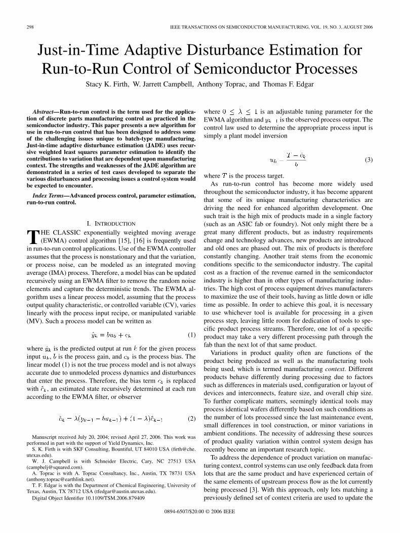
Fig. 1. Example of information grouping for feedback using control threads.

state in a control model similar to (1). The context criteria arechosen based on knowledge of the sources of variation of a givenprocess. These sets of equivalent context criteria are termed con-trol threads or streamlines. There exist as many values for thisstate term as there are possible combinations of the context cri-teria.

A simple example of the way in which information would begrouped for feedback with control threads is shown in Fig. 1.The context criteria are “tool” and “product” with two tools andthree products included in the control application. These criteriaresult in six groupings, or control threads, for feedback of infor-mation. Each of these threads has its own control model state,which is only updated using information from within that thread.The drawback to using control threads is evident when exam-ining how a disturbance in a context item is handled. Considera disturbance in Tool 1. Each of the three control threads ,

, and must experience and reject this disturbance sepa-rately because there is no information sharing between threads.So, when the disturbance occurs, the control thread can only“learn” about the disturbance when lots in this thread are run.The same is true for threads and , resulting in an adjust-ment period for each thread while each state is updated with thedisturbance information.

As a more realistic example, consider a typical fab where ap-proximately 150 different products are made [17]. A specificcontrol application in this fab may include two more contextcriteria in addition to “product,” such as “process tool,” the toolused in the current process step, and “previous process tool,” thetool on which the lot was run in the previous process step. Sup-pose that each of these criteria consists of five realizations. Inthis case, there would need to be over 3750 feedback loops for asingle application. Typically, a fab has an uneven mix of prod-ucts, where there are a few products which have many lots andmany products of which only a few lots are run. These so-calledlow-runner products present specific challenges to control sys-tems. In high-mix fabs with many products, some of the feed-back loops may operate with long time periods between datapoints in the feedback loop. This long delay results in a lossof information about the process tool contribution to the vari-ance in that specific product. The state of the process tool mayexperience drifts or shifts during the time period in betweenlow-runner product feedback loop data points. These changes tothe process tool state cannot be inferred by the controller stateuntil the next lot with the same context is run. At that time, thecontroller sees the process tool state change as a disturbance to

the particular feedback loop which must be rejected. Each feed-back loop must comprehend and reject this disturbance sepa-rately, because there is no sharing of information between feed-back loops.

Miller [11] characterized this problem and suggested the de-velopment of control systems that share decoupled informationamong tools and products. Recently, several authors have pro-posed solutions to the multiproduct control problem for bothchemical–mechanical polishing [6], [13] and photolithographyCD [20].

Pasadyn [12] used a Kalman filter method to perform stateestimation and control and to take into account the tools, prod-ucts, and processes within a process area. In this method, statesare assigned to each of these relevant context items within theprocess area and a state-space model formulation is used. Thestate error covariance matrix is then used with the Kalman filterto provide updates to the state estimates. One of the chief diffi-culties [12] is that of unobservability in the observer matrix. Thesolution put forth was the use of additional on-line experimentsto measure the separate states or reduce the number of states byadding constraints.

This paper details a new algorithm developed to address theissues raised with multiple process stream control in the semi-conductor industry. The algorithm, called just-in-time adaptivedisturbance estimation (JADE), is outlined and applied to sev-eral test cases designed to isolate typical types of process dis-turbances observed in the semiconductor industry.

II. JADE CONTROLLER DESIGN

The JADE algorithm is designed to estimate the error betweena control model and the semiconductor manufacturing processunder control. The proposed JADE algorithm includes a newtechnique for disturbance modeling by decoupling the processvariation and attributing each portion to the contributing contextitems, such as process tool, product, technology, reticle, etc. Aweighted recursive least squares estimation method is used toadaptively identify the contributions to variation from each in-dividual context item.

A. Process Model

The process model used by JADE for model-based control isof the same form as that for EWMA (1) with one minor modifi-cation. The bias term, or state, now represents the sum total ofall of the context-based states of the context items contributingto the variation for a particular lot. Including this modification,the JADE process model is

(4)

The bias term, , at each run , is defined as

(5)

where the summation is over the specific context items. Thistotal bias, or state, can be viewed as the superposition of thecontext-based bias from each of the contributing context items.


For example, (5) for photolithography overlay could be writtenas

(6)

so that the state is broken down into its components related to thespecific tool, reticle, reference tool, and reference reticle used toprocess each lot. In practice, these context categories (tool, ret-icle, etc.) would be chosen for inclusion in the algorithm basedon knowledge of the specific process and what is likely to be re-lated to significant disturbances to the process. JADE estimateseach of these component errors after each lot is processed.

B. Control Law

The control objective is to maintain the process output asclose to target as possible. Therefore, the JADE control al-gorithm also uses a plant model inversion for the control law,similar to (3) for the EWMA algorithm. The difference is thatthe single bias term estimate is replaced by the sum of thecontext-based error estimates for the relevant context items

(7)

(8)

As with the EWMA algorithm, the JADE algorithm uses a dead-beat (plant inverse) control law.

C. Observer

The bias component estimation can be thought of as a pa-rameter estimation. For individual context items (e.g., eachtool, reticle, etc.) and given runs such that all possible uniquecombinations of the individual context items are included, theresulting set of linear equations would be

(9)

where is an vector of context-based state estimates andis an vector of total observed biases, the components

of which are calculated from

(10)

The matrix in (9) is an matrix of ones and zeros forthe assignment of relevant context items for inclusion in the totalstate. The value of depends on the number of context items ineach context category, e.g., the number of tools in the category“tool,” and the number of context categories, e.g., “tool” and“reticle.” For example, given a reduced context of only two toolsand two reticles, would become

(11)

where columns 1, 2, 3, and 4 represent Tool 1, Tool 2, Reticle1, and Reticle 2, respectively. A one in a column corresponds tothe use of that context item in the lot corresponding to that row.For example, the lot for the first row was run using Tool 1 withReticle 1. Using a least squares method of parameter estimation,the solution of (9) is

(12)

In the general least squares problem, the number of observa-tions must be equal to or greater than the number ofvector variables to be estimated. However, the structure of ,as exemplified in (11) where , poses a further problem.The separate context items are confounded with one another, re-sulting in being rank deficient. Therefore, there is no longer aguarantee of uniqueness for the solution of (9) using these leastsquares methods even when the number of observations exceedsthe number of variables to be estimated. There are two ways toformulate such that it will have full rank in the limit: 1) makeuse of qualification runs, thereby adding more measurements,effectively adding linearly independent rows to and 2) makeuse of correlations between specific context items, effectivelyadding another equation and allowing a degree of freedom to beeliminated from the estimation procedure. In photolithography,the first condition can be accomplished by using tool qualifi-cation runs on so-called “golden” reference wafers to identifythe bias contribution from each of the tools and reference toolsused. These qualification runs are performed periodically, be-tween lots, during normal operation of a fab. The bias measure-ment from these qualification runs can be attributed directly tothe tool used. The periodic reuse of such golden wafers requiresthe wafers can be returned to their preprocess state, a capabilityparticular to the photolithography process and a further limita-tion of the golden wafer method. The second condition couldbe met if there is a high correlation between reticle and refer-ence reticle. The additional data and equations added into (9)will vary based on individual manufacturing practices.

Once (9) has been assembled such that has full rank, thequestion of how it may be used in practice arises. Keeping alldata necessary to construct the equation is not plausible becausedata storage and acquisition, as well as solution time, wouldrapidly become problematic. The time necessary to access avery large number of data points from a database and the com-putation to invert the resulting large matrix would be prohibitivefor a control application. However, it is not sufficient to simplyupdate (9) with new rows as runs are completed and measure-ments are made, while removing rows corresponding to old data.There is no guarantee in a manufacturing environment that runswill occur in an order such that the invertibility of willalways be assured.

A general method, here called the JADE algorithm, addressesthe issue of providing full rank without necessitating goldenwafer runs or requiring correlations between context items. Fora recursive update of the context-based state contributions, (9)may be truncated to a specified number of rows of the latestobservations and augmented as

(13)


where is an identity matrix and is the estimate of con-text-based state contributions for run . In this equation, the newestimates for the context-based biases are updated basedon new information in the latest runs and knowledge of the oldestimates . In this way, only the biases for the context itemsused in these latest runs are updated. Biases for context itemsnot used remain unchanged. The number of rows to keep in therecursive estimation is chosen by the user of the algorithm andcan be set to achieve best performance for a particular process.For simplicity in notation, define

(14)

which can be substituted into (13) to yield a more compact ex-pression

(15)

The augmenting of ensures the invertibility of . As withthe EWMA algorithm, it is assumed that the process to whichJADE will be applied is an IMA process. A weighting matrixis used as the means to assign preference to the current measure-ment versus past measurements and state contribution estimates.With the inclusion of this weighting matrix and the above sub-stitutions, an objective function can be written for the solutionof the JADE observer

(16)

is defined as

(17)

where is a matrix and is an matrix whosestructure is

......

. . .

......

. . .(18)

where is a tuning parameter to weight current state measure-ments against past context-based state estimates and the rep-resent relative weighting between the context-based state esti-mates. In general, it is not required that all be identical, butit is written as such for the sake of simplicity. Also, the morefreedom allowed in the number of tuning parameters, the morecomplicated the procedure of identification of those parametersbecomes. and are matrices of zeros with sizes and

, respectively. If the JADE algorithm is reduced to onecontext item and a sliding window of one lot ,it can be proven that the JADE and EMWA observers are equiv-alent under these conditions [8]. Equation (16) is solved for thecontext-based states using a least squares solution procedure,resulting in the following realization for the context-based stateestimates:

(19)

Equation (19) can be considered to be the observer for the JADEalgorithm. While each of the 1 to diagonal terms of and

in (18) assume a single-valued variable, in general, a dif-ferent value of could be used in each of the correspondingrows of and . Further, there is no mathematical require-ment for bounding in the EWMA sense between one and zero.In this paper, has been restricted to the same EWMA-boundedvalue in each row of and in order to retain analogousproperties to the widely implemented EWMA run-to-run con-trol algorithm.

At each iteration of JADE, (8) is solved, based on the totalbias estimated by JADE from the data previous to run , to ob-tain the input to be used in the process at run . When run iscompleted and the measurements are known, the actual bias forrun is calculated using (10). The individual biases to be usedin the calculations for run are then calculated using (19)and summed using (5). Using this procedure, the JADE algo-rithm is used to determine how the contributing context itemsmay be varying and how best to compensate for that variation.By segregating the states into the variation contributed by eachcontext item, the JADE algorithm does not suffer from the lackof information sharing experienced by threaded EWMA. JADEmore readily allows for full mix and match production.

III. SIMULATION DESCRIPTION

The following sections contain general test cases that are de-signed to give insight into the operation of JADE and to rep-resent aspects of processing conditions present in real applica-tions in the semiconductor industry. As a point of comparison,the EWMA algorithm, as the most prominent control algorithmused in industry, is also applied to the test cases.

The data for the case studies presented were generated viasimulation in order to isolate different aspects of processingand investigate their effects on the performance of the JADEand EWMA algorithms. The data were generated in such a waythat the actual context item variation and JADE calculated con-text item variation could be compared. Two values for each offour contexts were used for lot context, resulting in a total ofeight context items. Signals for each of the eight specific con-text items were generated separately using a possible combi-nation of two typical disturbances, step and ramp. The contextrealization for each lot was randomly selected based on a givenprobability of occurrence for the two choices in each of the fourcategories of context. The probability used for selection of thecontext items for each lot is shown in Table I. The total signalfor input into the controller was calculated by summing the in-dividual signals from the selected context items. This simulatedsignal was given to the JADE and EWMA algorithms to test


TABLE IPROBABILITY OF CONTEXT SELECTION FOR

JADE SIMULATIONS

how accurately each could estimate the total state using their re-spective observer [(2) and (19)]. For completeness, the EWMAalgorithm was also simulated without control threads for stepand ramp disturbances in Sections IV-A and IV-B, respectively.Unless otherwise specified, EWMA will refer to the threadedimplementation of the algorithm throughout the remainder ofthis paper. Both JADE and EWMA algorithms were run mul-tiple times to determine the optimal tuning for the set of inputdata. The results presented have been generated using the op-timal tuning for each algorithm.

The process model used to represent the actual process isshown as follows; the process is linear such that the processoutput is directly proportional to the process input:

(20)

Here, the bias or state is the quantity estimated by both theJADE and EWMA algorithms and is the process proportion-ality constant, or gain. Disturbances are injected into the stateof the process, which is modeled as

(21)

where , , , and represent the contexts included in themodel. These contexts can each take one of two realizations,dependent on the lot . This model is analogous to the statemodel that would be used for lithography where the contextsare tool, reticle, reference tool, and reference reticle and thereare two of each context available for use during processing.

The process model used by the controller is

(22)

where is the predicted output, is the controller processmodel gain, and is the estimated state. For all simulations,except those in Section V-A, and are equal. The sum ofsquared errors (SSE) between the process state and the state es-timated by the algorithm is used to demonstrate the ability ofthe control algorithm to correctly estimate the process state. Forlot , the squared error (SE) between the actual and estimatedstate is

SE (23)

The purpose of the simulations is to compare state estimatesonly and no feedback is provided. Since the base recipe settingsare assumed, , . The SSE is obtained by summing theSE over all lots

SSE SE (24)

Improvement in CV (or output) performance for semicon-ductor manufacturing is often measured by the increase in theprocess capability . is defined as the ratio of the spec-ification range to the process range corrected for noncenteringof the process around the target [10]. It is a statistical quantityused to measure how close the process mean is to the targetand how tight the process distribution is. Equation (25) is usedto calculate

LSL USL(25)

In this equation, LSL and USL are the lower and upper specifi-cation limits for the process and is the process standard devi-ation. An increase in indicates a movement of the processmean towards the target and a tightening of the process distri-bution.

IV. PROCESS DISTURBANCES

A disturbance to a process can be described as any occurrenceor series of occurrences that result in a change in the processingconditions. This disturbance is often not measurable; therefore,the disturbance information may not be available to the con-troller. The controller must reduce the effects of the disturbanceon the process output. In the sections that follow, we investigatethe influence of certain types of disturbances on the ability ofthe EWMA and JADE algorithms to accurately perform stateestimation. The goal is to minimize the deviation of the processoutput away from its setpoint.

A. Step Disturbance

The case where a context item undergoes a step disturbanceis investigated in this section. This type of disturbance is seenas an abrupt change in the context item’s contribution to thetotal state. For instance, such a disturbance might occur whena tool undergoes a maintenance event affecting the processingconditions. This event would be seen by the process as a stepdisturbance in the output variable.

Simulations were performed in which the value of one contextitem was changed from zero to a nonzero value abruptly, thusproducing the step disturbance. The value for context item ,i.e., context item number 1 of the context , was changed at the250th lot run using that context item. In the following plots, theactual number of total lots processed before this disturbance oc-curred resulted from the particular sequence of lots of randomlyselected context. In other words, the disturbance is observed at alater lot number because lots processed using both context items

and are included in the overall lot numbering sequence.The magnitude of the step was varied from a value of 0.01 to a


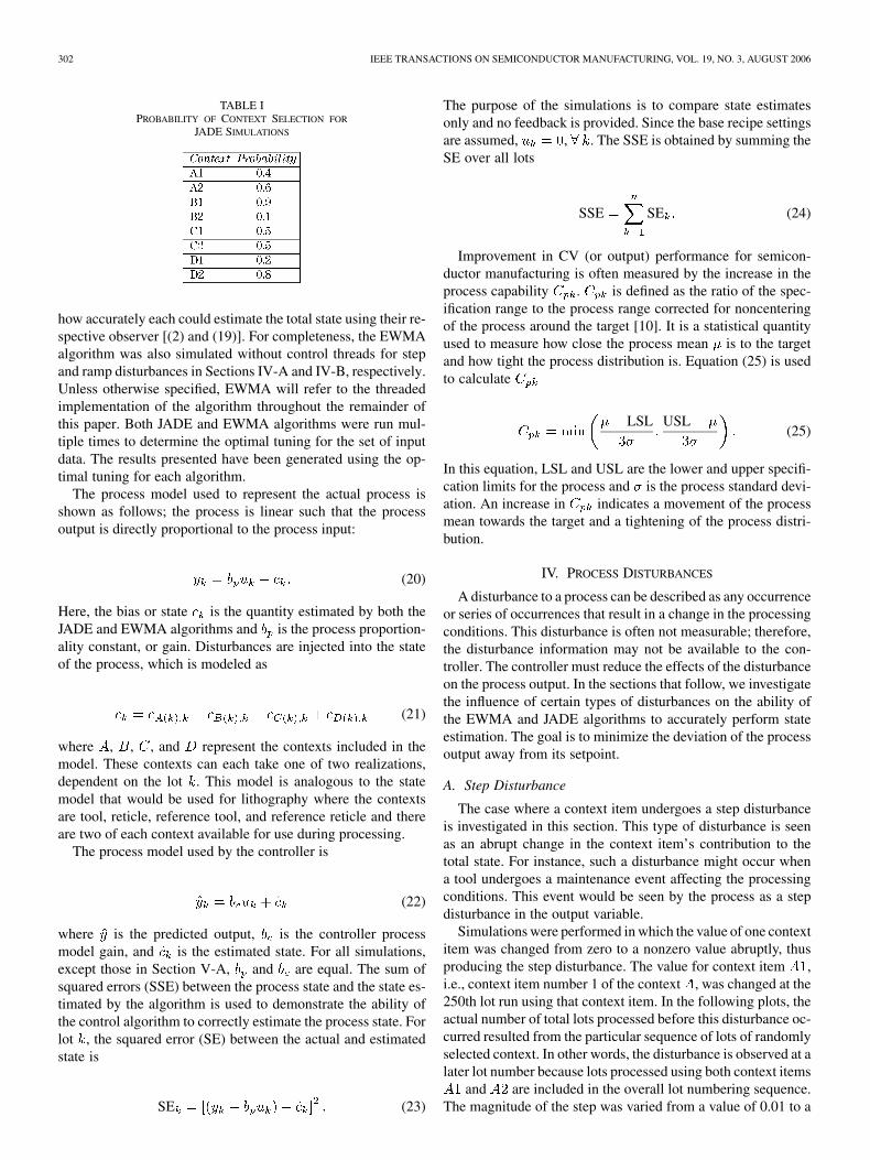
Fig. 2. Evolution of state with lot number for step disturbance in one context item.

value of 0.1. Signals for the other context items were held con-stant.

Fig. 2 shows the evolution of the JADE and EWMA estimatesof the state, as well as the actual state of the lots that includedcontext item for a simulation with a step of magnitude 0.05.From the figure, it can be observed that the step occurs at lotnumber 432. After the occurrence of the step disturbance, bothalgorithms “learn” about the disturbance.

The learning period for the JADE algorithm is characterizedby an initial change in signal from 0 to 0.05 with some damp-ening oscillation. The oscillation experienced by JADE is dueto the procedure of estimating the eight parameters in this sim-ulation. The threaded EWMA algorithm suffers from less oscil-lation; however, several spikes in the state are observed as eachthread containing context item is processed for the first timeafter the step disturbance. In the absence of noise, the threadedEWMA algorithm’s optimal tuning parameter is 1.0. There-fore, threaded EWMA can estimate a step disturbance in onelot. However, this step disturbance must be estimated for eachthread containing the context item undergoing the disturbance,resulting in the observed spikes. As the noise in the process in-creases, must decrease, in order to detune the controller andmake the controller less aggressive. A decrease in results in agreater number of lots required by each thread in the threadedEWMA algorithm to estimate a disturbance. So, with the ad-dition of process noise, the threaded EWMA algorithm perfor-mance would decrease further.

Because there are lots that do not contain the step distur-bance, the EWMA algorithm without threads is only able to

choose some operating point between 0 and 0.05. The re-sulting performance is poor when compared to threaded EWMAand JADE.

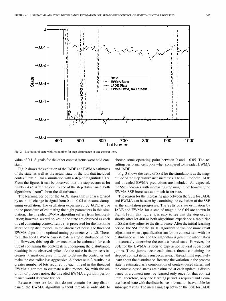
Fig. 3 shows the trend of SSE for the simulations as the mag-nitude of the step disturbance increases. The SSE for both JADEand threaded EWMA predictions are included. As expected,the SSE increases with increasing step magnitude; however, theEWMA SSE increases at a much faster rate.

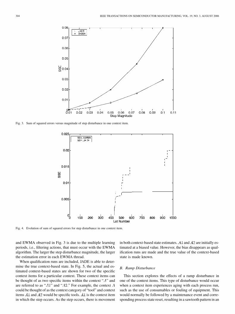
The reason for the increasing gap between the SSE for JADEand EWMA can be seen by examining the evolution of the SSEas the simulation progresses. The SSEs of state estimation byJADE and EWMA for a step of magnitude 0.05 are shown inFig. 4. From this figure, it is easy to see that the step occursshortly after lot 400 as both algorithms experience a rapid risein SSE as they adjust to the disturbance. After the initial learningperiod, the SSE for the JADE algorithm shows one more smalladjustment when a qualification run for the context item with thedisturbance is made and the algorithm is given the informationto accurately determine the context-based state. However, theSSE for the EWMA is seen to experience several subsequentjumps. These jumps occur each time a thread containing thestepped context item is run because each thread must separatelylearn about the disturbance. Because the variation in the processstate is estimated as a combination of context-based states, andthe context-based states are estimated at each update, a distur-bance in a context must be learned only once for that contextitem. Therefore, only one learning period is required and a con-text-based state with the disturbance information is available forsubsequent runs. The increasing gap between the SSE for JADE


Fig. 3. Sum of squared errors versus magnitude of step disturbance in one context item.

Fig. 4. Evolution of sum of squared errors for step disturbance in one context item.

and EWMA observed in Fig. 3 is due to the multiple learningperiods, i.e., filtering actions, that must occur with the EWMAalgorithm. The larger the step disturbance magnitude, the largerthe estimation error in each EWMA thread.

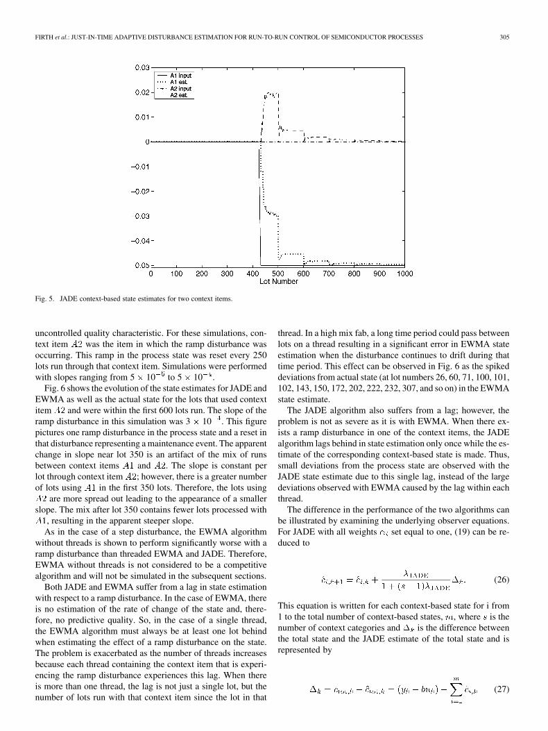
When qualification runs are included, JADE is able to deter-mine the true context-based state. In Fig. 5, the actual and es-timated context-based states are shown for two of the specificcontext items for a particular context. These context items canbe thought of as two specific items within the context “ ” andare referred to as “ ” and “ .” For example, the contextcould be thought of as the context category of “tool” and contextitems and would be specific tools. is the context itemin which the step occurs. As the step occurs, there is movement

in both context-based state estimates. and are initially es-timated at a biased value. However, the bias disappears as qual-ification runs are made and the true value of the context-basedstate is made known.

B. Ramp Disturbance

This section explores the effects of a ramp disturbance inone of the context items. This type of disturbance would occurwhen a context item experiences aging with each process run,such as the use of consumables or fouling of equipment. Thiswould normally be followed by a maintenance event and corre-sponding process state reset, resulting in a sawtooth pattern in an


Fig. 5. JADE context-based state estimates for two context items.

uncontrolled quality characteristic. For these simulations, con-text item was the item in which the ramp disturbance wasoccurring. This ramp in the process state was reset every 250lots run through that context item. Simulations were performedwith slopes ranging from 5 10 to 5 10 .

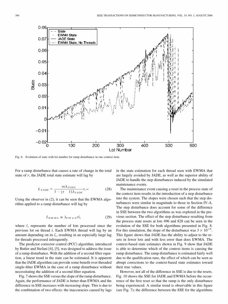
Fig. 6 shows the evolution of the state estimates for JADE andEWMA as well as the actual state for the lots that used contextitem and were within the first 600 lots run. The slope of theramp disturbance in this simulation was 3 10 . This figurepictures one ramp disturbance in the process state and a reset inthat disturbance representing a maintenance event. The apparentchange in slope near lot 350 is an artifact of the mix of runsbetween context items and . The slope is constant perlot through context item ; however, there is a greater numberof lots using in the first 350 lots. Therefore, the lots using

are more spread out leading to the appearance of a smallerslope. The mix after lot 350 contains fewer lots processed with

, resulting in the apparent steeper slope.As in the case of a step disturbance, the EWMA algorithm

without threads is shown to perform significantly worse with aramp disturbance than threaded EWMA and JADE. Therefore,EWMA without threads is not considered to be a competitivealgorithm and will not be simulated in the subsequent sections.

Both JADE and EWMA suffer from a lag in state estimationwith respect to a ramp disturbance. In the case of EWMA, thereis no estimation of the rate of change of the state and, there-fore, no predictive quality. So, in the case of a single thread,the EWMA algorithm must always be at least one lot behindwhen estimating the effect of a ramp disturbance on the state.The problem is exacerbated as the number of threads increasesbecause each thread containing the context item that is experi-encing the ramp disturbance experiences this lag. When thereis more than one thread, the lag is not just a single lot, but thenumber of lots run with that context item since the lot in that

thread. In a high mix fab, a long time period could pass betweenlots on a thread resulting in a significant error in EWMA stateestimation when the disturbance continues to drift during thattime period. This effect can be observed in Fig. 6 as the spikeddeviations from actual state (at lot numbers 26, 60, 71, 100, 101,102, 143, 150, 172, 202, 222, 232, 307, and so on) in the EWMAstate estimate.

The JADE algorithm also suffers from a lag; however, theproblem is not as severe as it is with EWMA. When there ex-ists a ramp disturbance in one of the context items, the JADEalgorithm lags behind in state estimation only once while the es-timate of the corresponding context-based state is made. Thus,small deviations from the process state are observed with theJADE state estimate due to this single lag, instead of the largedeviations observed with EWMA caused by the lag within eachthread.

The difference in the performance of the two algorithms canbe illustrated by examining the underlying observer equations.For JADE with all weights set equal to one, (19) can be re-duced to

(26)

This equation is written for each context-based state for i from1 to the total number of context-based states, , where is thenumber of context categories and is the difference betweenthe total state and the JADE estimate of the total state and isrepresented by

(27)


Fig. 6. Evolution of state with lot number for ramp disturbance in one context item.

For a ramp disturbance that causes a rate of change in the totalstate of , the JADE total state estimate will lag by

(28)

Using the observer in (2), it can be seen that the EWMA algo-rithm applied to a ramp disturbance will lag by

(29)

where represents the number of lots processed since theprevious lot on thread . Each EWMA thread will lag by anamount depending on its , resulting in an especially large lagfor threads processed infrequently.

The predictor corrector control (PCC) algorithm, introducedby Butler and Stefani [4], [5], was designed to address the issueof a ramp disturbance. With the addition of a second filter equa-tion, a linear trend in the state can be estimated. It is apparentthat the JADE algorithm can provide some benefit over threadedsingle-filter EWMA in the case of a ramp disturbance withoutnecessitating the addition of a second filter equation.

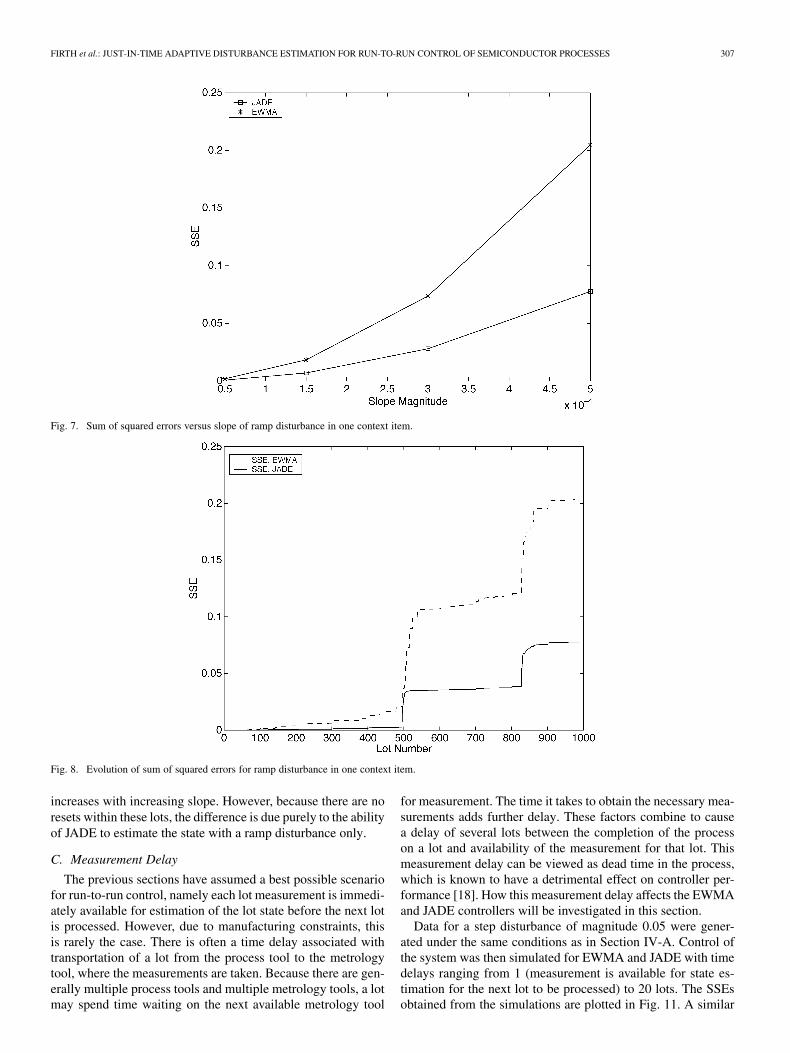
Fig. 7 shows the SSE versus the slope of the ramp disturbance.Again, the performance of JADE is better than EWMA and thedifference in SSE increases with increasing slope. This is due tothe combination of two effects: the inaccuracies caused by lags

in the state estimation for each thread seen with EWMA thatare largely avoided by JADE, as well as the superior ability ofJADE to handle the step disturbances induced by the simulatedmaintenance events.

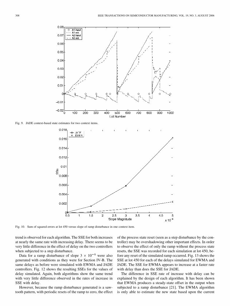
The maintenance event causing a reset in the process state ofthe context item results in the introduction of a step disturbanceinto the system. The slopes were chosen such that the step dis-turbances were similar in magnitude to those in Section IV-A.The step disturbance does account for some of the differencein SSE between the two algorithms as was explored in the pre-vious section. The effect of the step disturbance resulting fromthe process state resets at lots 496 and 828 can be seen in theevolution of the SSE for both algorithms presented in Fig. 8.For this simulation, the slope of the disturbance was 3 10 .This figure shows that JADE has the ability to adjust to the re-sets in fewer lots and with less error than does EWMA. Thecontext-based state estimates shown in Fig. 9 show that JADEis able to determine which of the context items is causing theramp disturbance. The ramp disturbance is estimated fairly welldue to the qualification runs, the effect of which can be seen asabrupt corrections to the context-based state estimates towardtheir true values.

However, not all of the difference in SSE is due to the resets.Fig. 10 shows the SSE for JADE and EWMA before the occur-rence of the first reset so that the ramp is the only disturbancebeing experienced. A similar trend is observable in this figure(see Fig. 7); the difference between the SSE for the algorithms


Fig. 7. Sum of squared errors versus slope of ramp disturbance in one context item.

Fig. 8. Evolution of sum of squared errors for ramp disturbance in one context item.

increases with increasing slope. However, because there are noresets within these lots, the difference is due purely to the abilityof JADE to estimate the state with a ramp disturbance only.

C. Measurement Delay

The previous sections have assumed a best possible scenariofor run-to-run control, namely each lot measurement is immedi-ately available for estimation of the lot state before the next lotis processed. However, due to manufacturing constraints, thisis rarely the case. There is often a time delay associated withtransportation of a lot from the process tool to the metrologytool, where the measurements are taken. Because there are gen-erally multiple process tools and multiple metrology tools, a lotmay spend time waiting on the next available metrology tool

for measurement. The time it takes to obtain the necessary mea-surements adds further delay. These factors combine to causea delay of several lots between the completion of the processon a lot and availability of the measurement for that lot. Thismeasurement delay can be viewed as dead time in the process,which is known to have a detrimental effect on controller per-formance [18]. How this measurement delay affects the EWMAand JADE controllers will be investigated in this section.

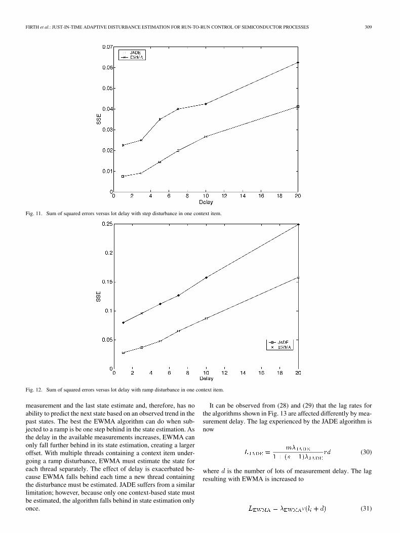
Data for a step disturbance of magnitude 0.05 were gener-ated under the same conditions as in Section IV-A. Control ofthe system was then simulated for EWMA and JADE with timedelays ranging from 1 (measurement is available for state es-timation for the next lot to be processed) to 20 lots. The SSEsobtained from the simulations are plotted in Fig. 11. A similar


Fig. 9. JADE context-based state estimates for two context items.

Fig. 10. Sum of squared errors at lot 450 versus slope of ramp disturbance in one context item.

trend is observed for each algorithm. The SSE for both increasesat nearly the same rate with increasing delay. There seems to bevery little difference in the effect of delay on the two controllerswhen subjected to a step disturbance.

Data for a ramp disturbance of slope 3 10 were alsogenerated with conditions as they were for Section IV-B. Thesame delays as before were simulated with EWMA and JADEcontrollers. Fig. 12 shows the resulting SSEs for the values ofdelay simulated. Again, both algorithms show the same trendwith very little difference observed in the rates of increase inSSE with delay.

However, because the ramp disturbance generated is a saw-tooth pattern, with periodic resets of the ramp to zero, the effect

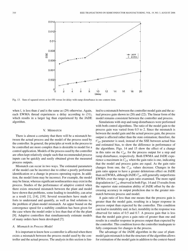
of the process state reset (seen as a step disturbance by the con-troller) may be overshadowing other important effects. In orderto observe the effect of only the ramp without the process stateresets, the SSE was recorded for each simulation at lot 450, be-fore any reset of the simulated ramp occurred. Fig. 13 shows theSSE at lot 450 for each of the delays simulated for EWMA andJADE. The SSE for EWMA appears to increase at a faster ratewith delay than does the SSE for JADE.

The difference in SSE rate of increase with delay can beexplained by the design of each algorithm. It has been shownthat EWMA produces a steady-state offset in the output whensubjected to a ramp disturbance [21]. The EWMA algorithmis only able to estimate the new state based upon the current


Fig. 11. Sum of squared errors versus lot delay with step disturbance in one context item.

Fig. 12. Sum of squared errors versus lot delay with ramp disturbance in one context item.

measurement and the last state estimate and, therefore, has noability to predict the next state based on an observed trend in thepast states. The best the EWMA algorithm can do when sub-jected to a ramp is be one step behind in the state estimation. Asthe delay in the available measurements increases, EWMA canonly fall further behind in its state estimation, creating a largeroffset. With multiple threads containing a context item under-going a ramp disturbance, EWMA must estimate the state foreach thread separately. The effect of delay is exacerbated be-cause EWMA falls behind each time a new thread containingthe disturbance must be estimated. JADE suffers from a similarlimitation; however, because only one context-based state mustbe estimated, the algorithm falls behind in state estimation onlyonce.

It can be observed from (28) and (29) that the lag rates forthe algorithms shown in Fig. 13 are affected differently by mea-surement delay. The lag experienced by the JADE algorithm isnow

(30)

where is the number of lots of measurement delay. The lagresulting with EWMA is increased to

(31)


Fig. 13. Sum of squared errors at lot 450 versus lot delay with ramp disturbance in one context item.

when is less than and is the same as (29) otherwise. Again,each EWMA thread experiences a delay according to (31),which results in a larger lag than experienced by the JADEalgorithm.

V. MISMATCH

There is almost a certainty that there will be a mismatch be-tween the actual process and the model of the process used bythe controller. In general, the principles at work in the process tobe controlled are more complex than is desirable to model for acontrol application. Models of the process used by the controllerare often kept relatively simple such that recommended processinputs can be quickly and easily obtained given the measuredprocess outputs.

Mismatch can occur in two ways. The estimated parametersof the model can be incorrect due to either a poorly performedidentification or a change in process operating region. In addi-tion, the model form may be incorrect. For example, the modelmay be linear, whereas significant nonlinearities may exist in theprocess. Studies of the performance of adaptive control whenthere exists structural mismatch between the plant and modelhave shown that problems, some leading to instability, can ariseas a result [1], [14], [19]. Several researchers have made ef-forts to understand and quantify, as well as find solutions to,the problem of plant-model mismatch. An upper bound on theconvergence speed for a stability condition has been given forthe case where the model order is less than that of the the plant[9]. Adaptive controllers that simultaneously estimate modelsof many orders have been developed [7].

A. Mismatch in Process Model

It is important to know how a controller is affected when thereexists a mismatch between the process model used by the con-troller and the actual process. The analysis in this section is lim-

ited to a mismatch between the controller model gain and the ac-tual process gain shown in (20) and (22). The linear form of themodel remains consistent between the controller and process.

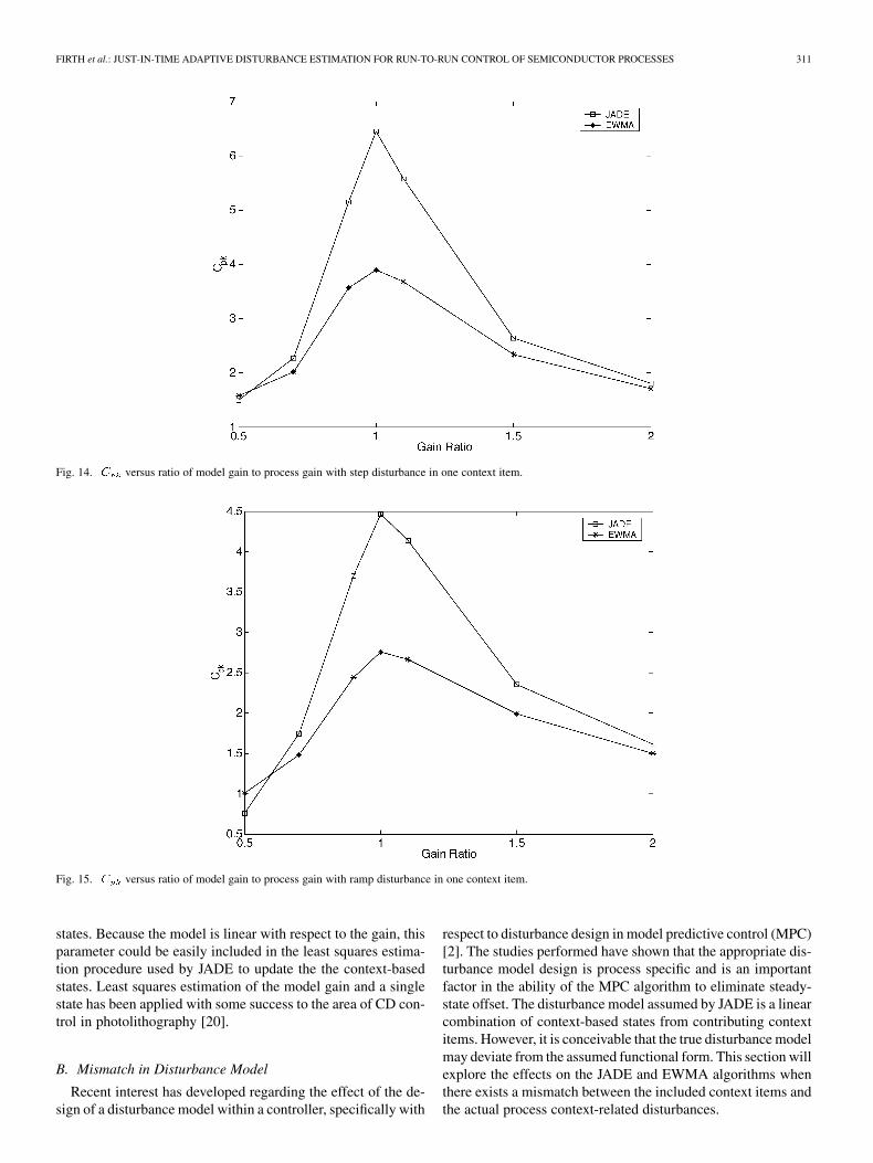
Simulations with step and ramp disturbances were performedwith both control algorithms. The ratio of the model gain to theprocess gain was varied from 0.5 to 2. Since the mismatch isbetween the model gain and the actual process gain, the processoutput is affected rather than the state estimation; therefore, the

parameter is used, instead of the SSE between actual biasand estimated bias, to show the difference in performance ofthe algorithms. Figs. 14 and 15 show the effect of a changein this ratio on the for the process output for a step andramp disturbance, respectively. Both EWMA and JADE expe-rience a maximum in when the gain ratio is one, indicatingthat the model and process gains are equal. As the gain ratiochanges from one, the values decrease. Changes in thegain ratio appear to have a greater deleterious effect on JADEthan on EWMA, although JADE still generally outperformsEWMA over the range in gain ratio examined. The more rapiddegradation in observed in both Figs. 14 and 15 results fromthe superior state estimation ability of JADE offset by the de-creasing accuracy in output prediction due to the greater mis-match between process and model.

A gain ratio of less than one means that the process gain isgreater than the model gain, resulting in a larger response inprocess output than expected by the controller. This conditioncan lead to instability and, in fact, instability in the response wasobserved for ratios of 0.5 and 0.7. A process gain that is lessthan the model gain gives a gain ratio of greater than one andresults in a smaller response in process output than expected bythe controller. This condition leaves the controller inadequate tofully compensate for changes in the process.

The advantage of the JADE algorithm in the case of plant-model gain mismatch is that the structure of the algorithm allowsfor estimation of the model gain in addition to the context-based


Fig. 14. C versus ratio of model gain to process gain with step disturbance in one context item.

Fig. 15. C versus ratio of model gain to process gain with ramp disturbance in one context item.

states. Because the model is linear with respect to the gain, thisparameter could be easily included in the least squares estima-tion procedure used by JADE to update the the context-basedstates. Least squares estimation of the model gain and a singlestate has been applied with some success to the area of CD con-trol in photolithography [20].

B. Mismatch in Disturbance Model

Recent interest has developed regarding the effect of the de-sign of a disturbance model within a controller, specifically with

respect to disturbance design in model predictive control (MPC)[2]. The studies performed have shown that the appropriate dis-turbance model design is process specific and is an importantfactor in the ability of the MPC algorithm to eliminate steady-state offset. The disturbance model assumed by JADE is a linearcombination of context-based states from contributing contextitems. However, it is conceivable that the true disturbance modelmay deviate from the assumed functional form. This section willexplore the effects on the JADE and EWMA algorithms whenthere exists a mismatch between the included context items andthe actual process context-related disturbances.


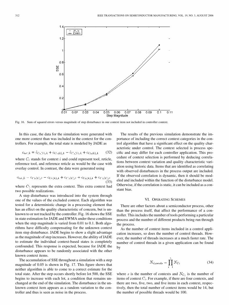
Fig. 16. Sum of squared errors versus magnitude of step disturbance in one context item not included in controller context.

In this case, the data for the simulation were generated withone more context than was included in the context for the con-trollers. For example, the total state is modeled by JADE as

(32)

where stands for context and could represent tool, reticle,reference tool, and reference reticle as would be the case withoverlay control. In contrast, the data were generated using

(33)where represents the extra context. This extra context hadtwo possible realizations.

A step disturbance was introduced into the system throughone of the values of the excluded context. Each algorithm wastested for a deterministic change in a processing element thathas an effect on the quality characteristic of concern, but is un-known to or not tracked by the controller. Fig. 16 shows the SSEin state estimation for JADE and EWMA under these conditionswhen the step magnitude is varied from 0.01 to 0.1. Both algo-rithms have difficulty compensating for the unknown contextitem step disturbance. JADE begins to show a slight advantageas the magnitude of step increases. However, the ability of JADEto estimate the individual context-based states is completelyconfounded. This response is expected, because for JADE thedisturbance appears to be randomly associated with the otherknown context items.

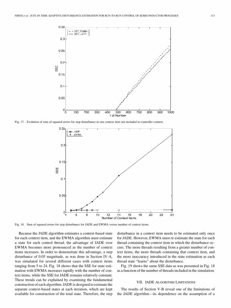
The accumulation of SSE throughout a simulation with a stepmagnitude of 0.05 is shown in Fig. 17. This figure shows thatneither algorithm is able to come to a correct estimate for thetotal state. After the step occurs shortly before lot 500, the SSEbegins to increase with each lot, a condition that remains un-changed at the end of the simulation. The disturbance in the un-known context item appears as a random variation to the con-troller and thus is seen as noise in the process.

The results of the previous simulation demonstrate the im-portance of including the correct context categories in the con-trol algorithm that have a significant effect on the quality char-acteristic under control. The context selected is process spe-cific and may differ for each controller application. This pro-cedure of context selection is performed by deducing correla-tions between context variation and quality characteristic vari-ation using historic data. Items that are identified as correlatingwith observed disturbances in the process output are included.If the observed correlation is dynamic, then it should be mod-eled and included within the function of the disturbance model.Otherwise, if the correlation is static, it can be included as a con-stant bias.

VI. OPERATING SCHEMES

There are other factors about a semiconductor process, otherthan the process itself, that affect the performance of a con-troller. This includes the number of tools performing a particularprocess and the number of different products being run throughthe process.

As the number of context items included in a control appli-cation increases, so does the number of control threads. How-ever, the number of threads increases at a much faster rate. Thenumber of control threads in a given application can be foundby

(34)

where is the number of contexts and is the number ofitems of context . For example, if there are four contexts, andthere are two, five, two, and five items in each context, respec-tively, then the total number of context items would be 14, butthe number of possible threads would be 100.


Fig. 17. Evolution of sum of squared errors for step disturbance in one context item not included in controller context.

Fig. 18. Sum of squared errors for step disturbance for JADE and EWMA versus number of context items.

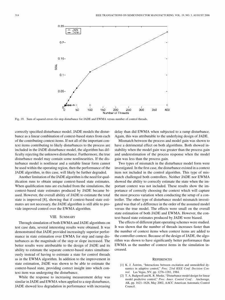
Because the JADE algorithm estimates a context-based statefor each context item, and the EWMA algorithm must estimatea state for each control thread, the advantage of JADE overEWMA becomes more pronounced as the number of contextitems increases. In order to demonstrate this advantage, a stepdisturbance of 0.05 magnitude, as was done in Section IV-A,was simulated for several different cases with context itemsranging from 5 to 24. Fig. 18 shows that the SSE for state esti-mation with EWMA increases rapidly with the number of con-text items, while the SSE for JADE remains relatively constant.These trends can be explained by examining the fundamentalconstruction of each algorithm. JADE is designed to estimate theseparate context-based states at each iteration, which are keptavailable for construction of the total state. Therefore, the step

disturbance in a context item needs to be estimated only oncefor JADE. However, EWMA must re-estimate the state for eachthread containing the context item in which the disturbance oc-curs. The more threads resulting from a greater number of con-text items, the more threads containing that context item, andthe more inaccuracy introduced in the state estimation as eachthread state “learns” about the disturbance.

Fig. 19 shows the same SSE data as was presented in Fig. 18as a function of the number of threads included in the simulation.

VII. JADE ALGORITHM LIMITATIONS

The results of Section V-B reveal one of the limitations ofthe JADE algorithm—its dependence on the assumption of a


Fig. 19. Sum of squared errors for step disturbance for JADE and EWMA versus number of control threads.

correctly specified disturbance model. JADE models the distur-bance as a linear combination of context-based states from eachof the contributing context items. If not all of the important con-text items contributing to likely disturbances to the process areincluded in the JADE disturbance model, the algorithm has dif-ficulty rejecting the unknown disturbance. Furthermore, the truedisturbance model may contain some nonlinearities. If the dis-turbance model is nonlinear and a suitable linear form cannotbe used within the operating region, then the performance of theJADE algorithm, in this case, will likely be further degraded.

Another limitation of the JADE algorithm is the need for qual-ification runs to obtain unique context-based state estimates.When qualification runs are excluded from the simulations, thecontext-based state estimates produced by JADE became bi-ased. However, the overall ability of JADE to estimate the totalstate is improved [8], showing that if context-based state esti-mates are not necessary, the JADE algorithm is still able to pro-vide improved control over the EWMA algorithm.

VIII. SUMMARY

Through simulation of both EWMA and JADE algorithms ontest case data, several interesting results were obtained. It wasdemonstrated that JADE provided increasingly superior perfor-mance in state estimation over EWMA for step and ramp dis-turbances as the magnitude of the step or slope increased. Thebetter results were attributable to the design of JADE and itsability to estimate the separate context-based states simultane-ously instead of having to estimate a state for control threadsas in the EWMA algorithm. In addition to the improvement instate estimation, JADE was shown to be able to estimate thecontext-based state, providing correct insight into which con-text item was undergoing the disturbance.

While the response to increasing measurement delay wassimilar in JADE and EWMA when applied to a step disturbance,JADE showed less degradation in performance with increasing

delay than did EWMA when subjected to a ramp disturbance.Again, this was attributable to the underlying design of JADE.

Mismatch between the process and model gain was shown tohave a detrimental effect on both algorithms. Both showed in-stability when the model gain was greater than the process gainand underestimation of the process response when the modelgain was less than the process gain.

Two types of mismatch in the disturbance model form wereinvestigated. In the first case, the disturbance existed in a contextitem not included in the control algorithm. This type of mis-match challenged both controllers. Neither JADE nor EWMAshowed the ability to correctly estimate the state when the im-portant context was not included. These results show the im-portance of correctly choosing the context which will capturethe most process variation when conducting the setup of a con-troller. The other type of disturbance model mismatch investi-gated was that of a difference in the order of the assumed modelversus the true model. The effects were small on the overallstate estimation of both JADE and EWMA. However, the con-text-based state estimates produced by JADE were biased.

The effects of different plant operating schemes were studied.It was shown that the number of threads increases faster thanthe number of context items when context items are added tothe controller context. Because of the design of JADE, the algo-rithm was shown to have significantly better performance thanEWMA as the number of context items in the simulation in-creased.

REFERENCES

[1] K. J. Åström, “Interactions between excitation and unmodelled dy-namics in adaptive control,” Proc. 23rd IEEE Conf. Decision Con-trol. Las Vegas, NV, pp. 1276–1281, 1984.

[2] T. A. Badgwell and K. R. Muske, “Disturbance model design for linearmodel predictive control,” Proc. Amer. Control Conf.. Anchorage,AK, pp. 1621–1626, May 2002, AACC American Automatic ControlCouncil.


[3] C. A. Bode, “Run-to-Run control of overlay and linewidth in semicon-ductor manufacturing,” Ph.D. dissertation, Univ. Texas, Austin, 2001.

[4] S. W. Butler, “Texas Instruments’ overview of control needs for man-ufacturing in the 90’s,” in Proc. AEC/APC Workshop V. SEMATECH,Oct. 1993.

[5] S. W. Butler and J. A. Stefani, “Supervisory run-to-run control ofpolysilicon gate etch using in situ ellipsometry,” IEEE Trans. Semi-conduct. Manufact., vol. 7, no. 2, pp. 193–201, May 1994.

[6] W. J. Campbell, “Model predictive run-to-run control of chemical me-chanical planarization,” Ph.D. dissertation, Univ. Texas, Austin, 1999.

[7] D. W. Clarke, “Adaptive predictive control,” Annu. Rev. Contr., vol.20, pp. 83–94, 1996.

[8] S. K. Firth, “Just-in-Time adaptive disturbance estimation forrun-to-run control in semiconductor processes,” Ph.D. dissertation,Univ. Texas, Austin, 2002.

[9] Y. Fu and G. A. Dumont, “A stability condition for STCwith model mismatch,” Proc. 26th Conf. Decision Control pp.1555–1560. Tampa, FL, Dec. 1989.

[10] S. Kotz and C. R. Lovelace, Process Capability Indices in Theory andPractice. New York: Edward Arnold, 1998.

[11] M. L. Miller, “Use of scatterometric measurements for control ofphotolithography,” Ph.D. dissertation, Univ. California, Santa Barbara,1994.

[12] A. J. Pasadyn, “Simultaneous control and identification for multipleproduct and process environments in semiconductor manufacturing,”Ph.D. dissertation, Univ. Texas, Austin, 2001.

[13] N. S. Patel, G. A. Miller, C. Guinn, A. C. Sanchez, and S. T. Jenkins,“Device dependent control of chemical-mechanical polishing of dielec-tric films,” IEEE Trans. Semiconduct. Manufact., vol. 13, no. 3, pp.331–343, Aug. 2000.

[14] C. Rohrs, L. Valavani, M. Athans, and G. Stein, “Robustness of con-tinuous-time adaptive control algorithms in the presence of unmodeleddynamics,” IEEE Trans. Automat. Contr., vol. AC-30, pp. 881–889,1985.

[15] E. Sachs, S. Ha, A. Hu, and W. Metz, “Automated on-line optimizationof an epitaxial process,” Proc. Semiconductor Manufacturing ScienceSymp. IEEE/SEMI, 1990.

[16] E. Sachs, A. Hu, A. Ingolfsson, and P. H. Langer, “Modeling and con-trol of an epitaxial silicon deposition process with step disturbances,”in Proc. IEEE/SEMI Advanced Semiconductor Manufacturing Conf.,1991.

[17] J. Schmitz, “A view on advanced control techniques from a wafer fabmanager’s perspective,” in Proc. 3rd Eur. AEC/APC Conf., Apr. 2002.

[18] D. E. Seborg, T. F. Edgar, and D. A. Mellichamp, Process Dynamicsand Control, 2nd ed. New York: Wiley, 2004.

[19] D. E. Seborg, T. F. Edgar, and S. L. Shah, “Adaptive control strategiesfor process control: A survey,” AIChE J., vol. 32, no. 6, pp. 881–913,Jun. 1986.

[20] J. D. Stuber, F. Pagette, and S. Tang, “Device dependent run-to-run con-trol of transistor critical dimension by manipulating photolithogralhyexposure settings,” B. Van Eck, Ed., Proc. AEC/APC Symp. XII vol. I,Int. SEMATECH, 2000.

[21] A. J. Toprac, S. K. Firth, and W. J. Campbell, “Tutorial: Compar-ison of run-to-run control algorithms,” Proc. AEC/APC Symp. XIII SE-MATECH, Oct. 2001.

Stacy K. Firth received the B.S. and M.S. degreesfrom the University of Utah, in 1995 and 1998, re-spectively. She received the Ph.D. degree in chemicalengineering from the University of Texas, Austin, in2002, under the direction of Dr. T. F. Edgar.

She worked as a Research Engineer for Yield Dy-namics, Inc., for two years, during which time her re-search resulted in two patents. She currently consultsprivately.

W. Jarrett Campbell received the Ph.D. degree inchemical engineering (with an emphasis on advancedprocess control (APC) applied to semiconductor pro-cesses) from the University of Texas, Austin, in 1999.

He is a Strategic Marketing Manager at SchneiderElectric, Cary, NC. He has more than nine years expe-rience applying APC solutions in the semiconductorindustry including former positions as a Member ofthe Technical Staff at both Advanced Micro Devices(AMD) and Yield Dynamics and as the Process Con-trol Engineering Manager at KLA-Tencor. During his

career, he has developed and overseen the deployment of APC solutions in theareas of chimical–mechanical polishing, etch, deposition, and lithography. Hehas been granted 21 U.S. patents and has published over 20 articles in the areaof APC and semiconductor manufacturing.

Anthony Toprac received the Ph.D. degree in chem-ical engineering from the University of Texas, Austin.

He is Principal of A. Toprac Consultancy, Inc., aprivate consulting firm specializing in manufacturingcontrol systems. He is the author of numerous publi-cations and patents in the area of process control insemiconductor processing and is a registered Profes-sional Engineer in the state of Texas.

Thomas F. Edgar received the B.S.Ch.E. degreefrom the University of Kansas and Ph.D. degreefrom Princeton University, Princeton, NJ, in 1971.

He is a Professor of chemical engineering at theUniversity of Texas, Austin. His research interests in-clude the areas of process modeling, control, and op-timization.

just-in-time adaptive disturbance estimation for run-to-run control of semiconductor processes

Documents