junction trees: motivation standard algorithms (e.g., variable elimination) are inefficient if the...
TRANSCRIPT
Junction Trees: Motivation
• Standard algorithms (e.g., variable elimination) are inefficient if the undirected graph underlying the Bayes Net contains cycles.
• We can avoid cycles if we turn highly-interconnected subsets of the nodes into “supernodes.”
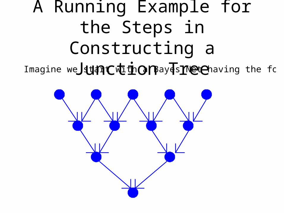
A Running Example for the Steps in Constructing a Junction Tree
Imagine we start with a Bayes Net having the following structure.
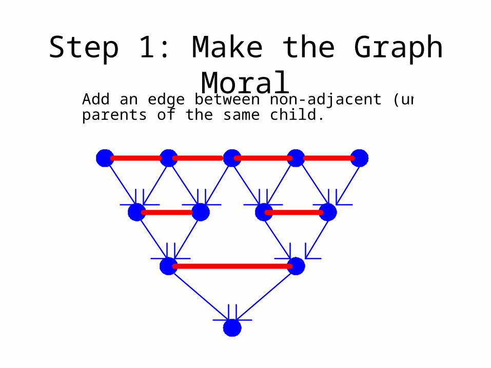
Step 1: Make the Graph MoralAdd an edge between non-adjacent (unmarried)parents of the same child.
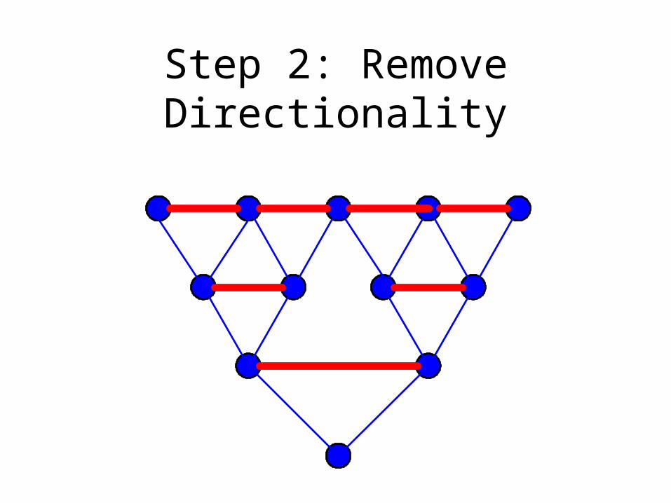
Step 2: Remove Directionality

Step 3: Triangulate the GraphRepeat while there exists a cycle of length > 3 with no chord:
Add a chord (edge between two non-adjacentvertices in such a cycle).
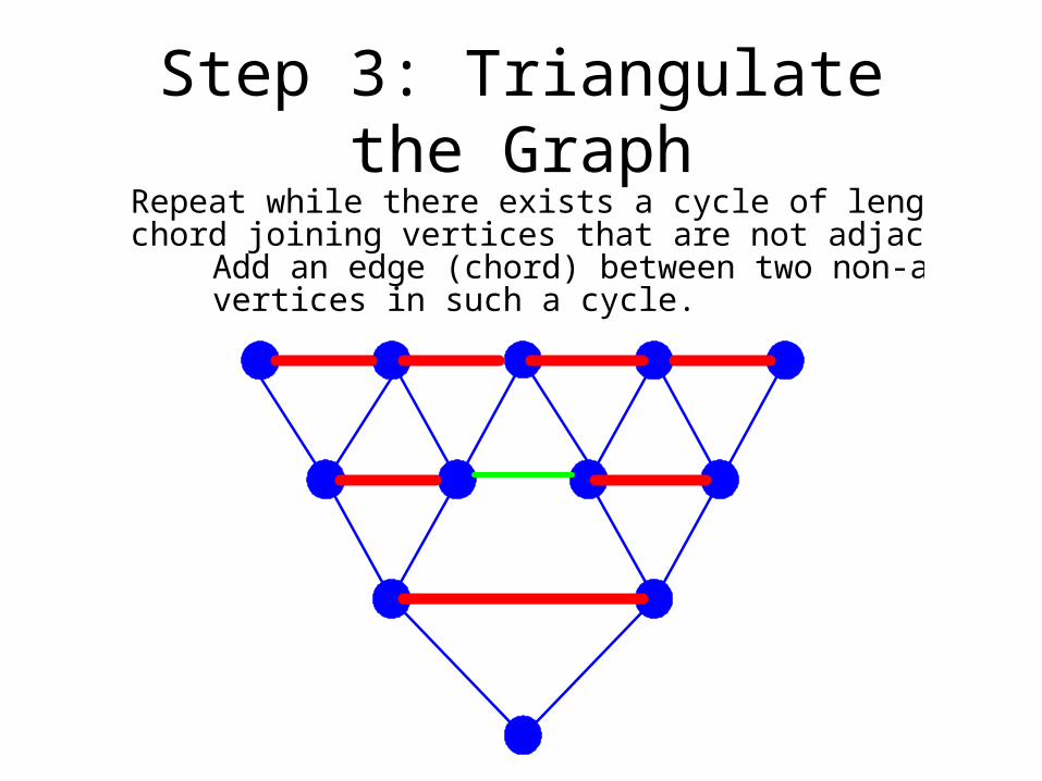
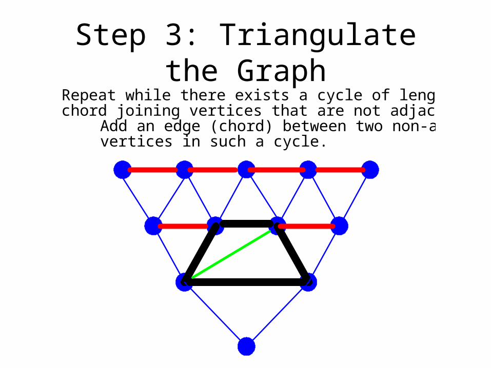
Step 3: Triangulate the GraphRepeat while there exists a cycle of length > 3 with nochord joining vertices that are not adjacent in the cycle:
Add an edge (chord) between two non-adjacentvertices in such a cycle.
Step 3: Triangulate the GraphRepeat while there exists a cycle of length > 3 with nochord joining vertices that are not adjacent in the cycle:
Add an edge (chord) between two non-adjacentvertices in such a cycle.

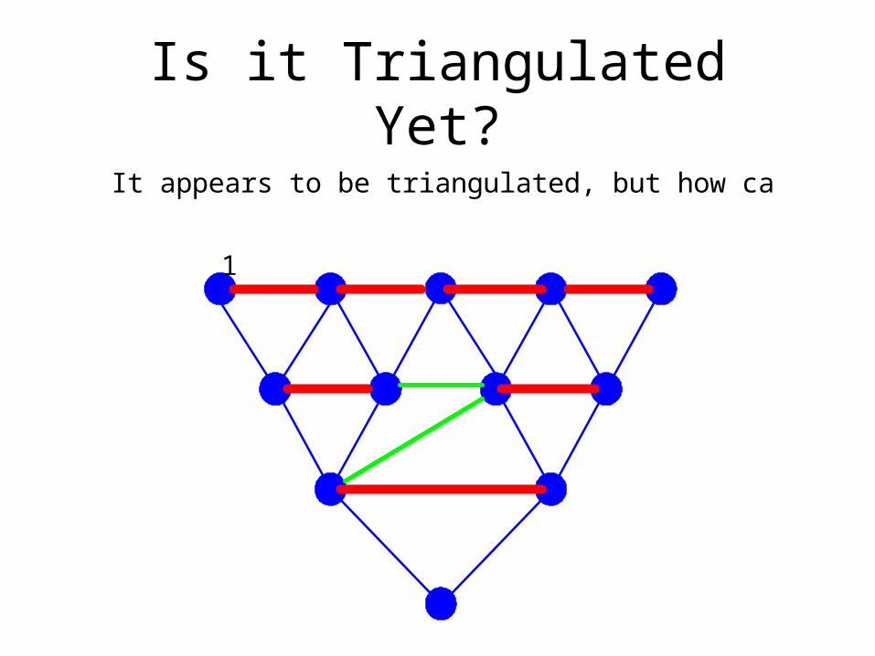
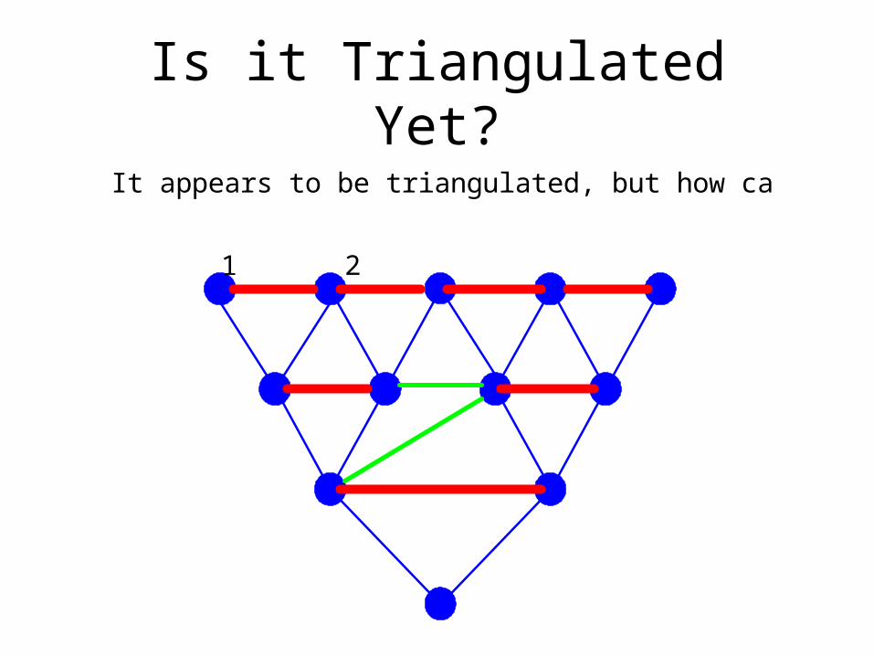
Is it Triangulated Yet?
It appears to be triangulated, but how can we be sure?
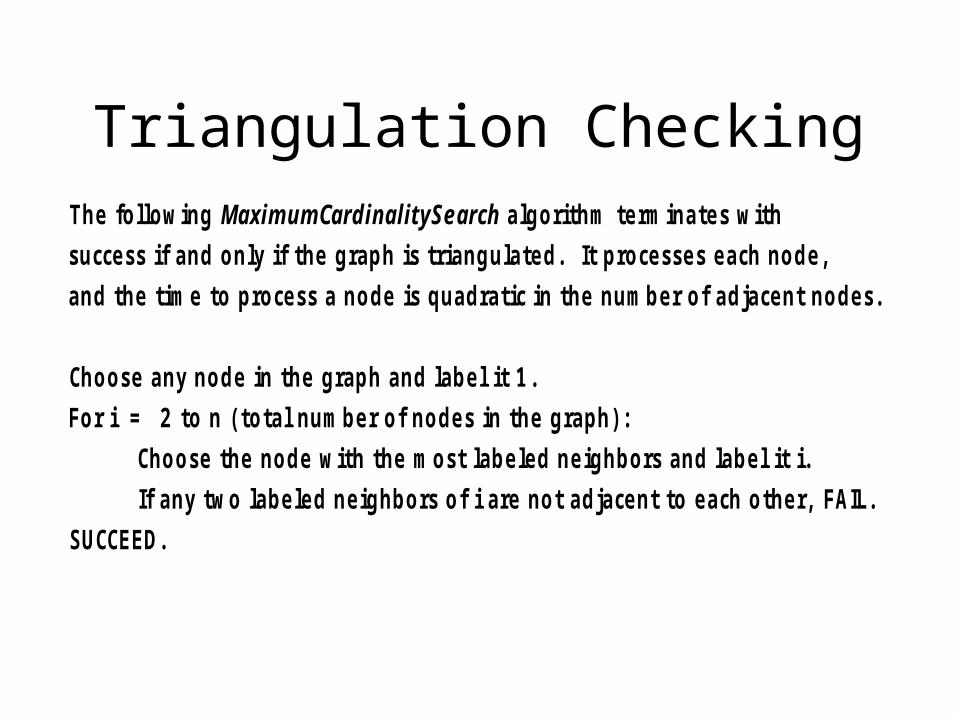
Triangulation CheckingThe following algorithm terminates with
success if and only if the graph is triangulated. It processes each node,
and the time to process a node is quadratic in the number of adjacent nodes.
Choose any node in the graph and label it 1.
For i = 2 to n ( total number of nodes in the graph) :
Choose the node with the most labeled neighbors and label it i.
If any two labeled neighbors of i are not adjacent to each other, FAIL.
SUCCEED.
MaximumCardinalitySearch
Is it Triangulated Yet?
It appears to be triangulated, but how can we be sure?
1
Is it Triangulated Yet?
It appears to be triangulated, but how can we be sure?
1 2

Is it Triangulated Yet?
It appears to be triangulated, but how can we be sure?
1 2
3

Is it Triangulated Yet?
It appears to be triangulated, but how can we be sure?
1 2
3 4
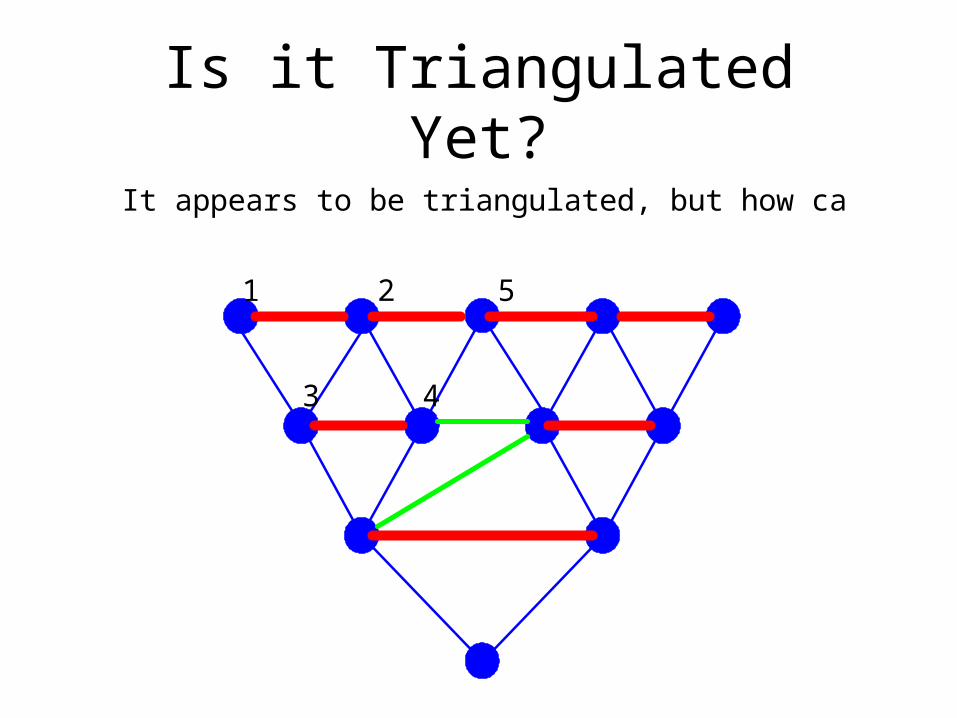
Is it Triangulated Yet?
It appears to be triangulated, but how can we be sure?
1 2
3 4
5

Is it Triangulated Yet?
It appears to be triangulated, but how can we be sure?
1 2
3 4
5
6
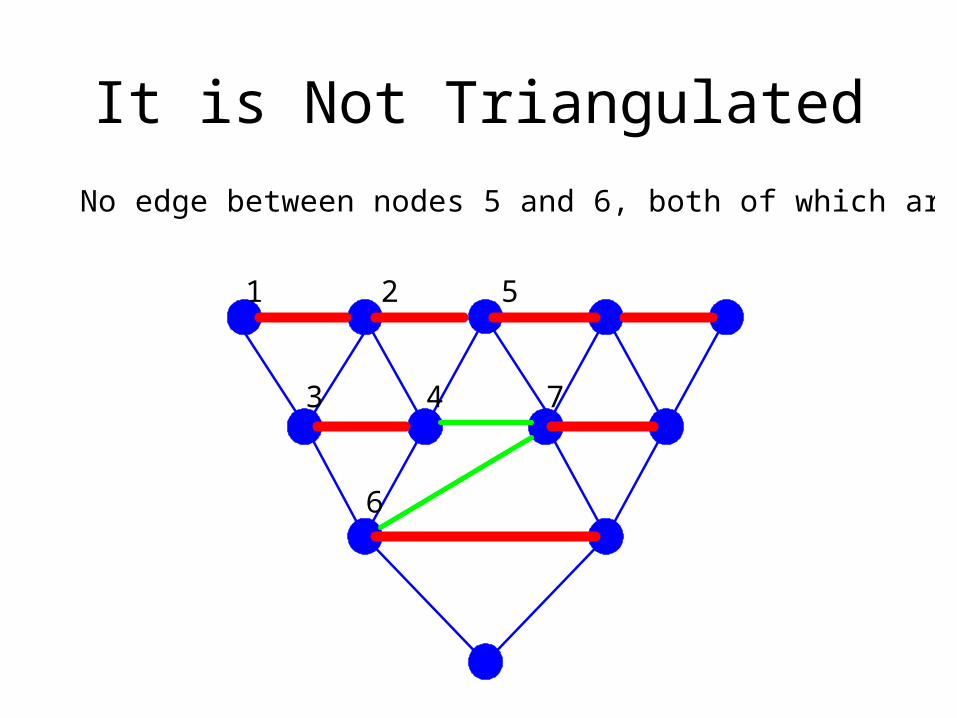
It is Not Triangulated
No edge between nodes 5 and 6, both of which are parents of 7.
1 2
3 4
5
6
7
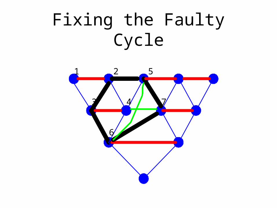
Fixing the Faulty Cycle
1 2
3 4
5
6
7
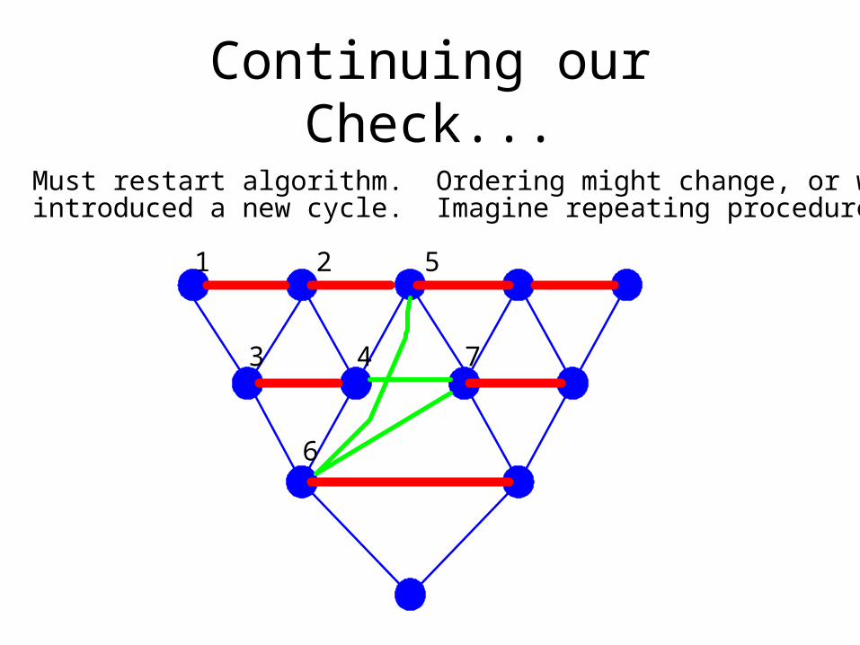
Continuing our Check...
Must restart algorithm. Ordering might change, or we might have.
1 2
3 4
5
6
7
introduced a new cycle. Imagine repeating procedure with this graph.
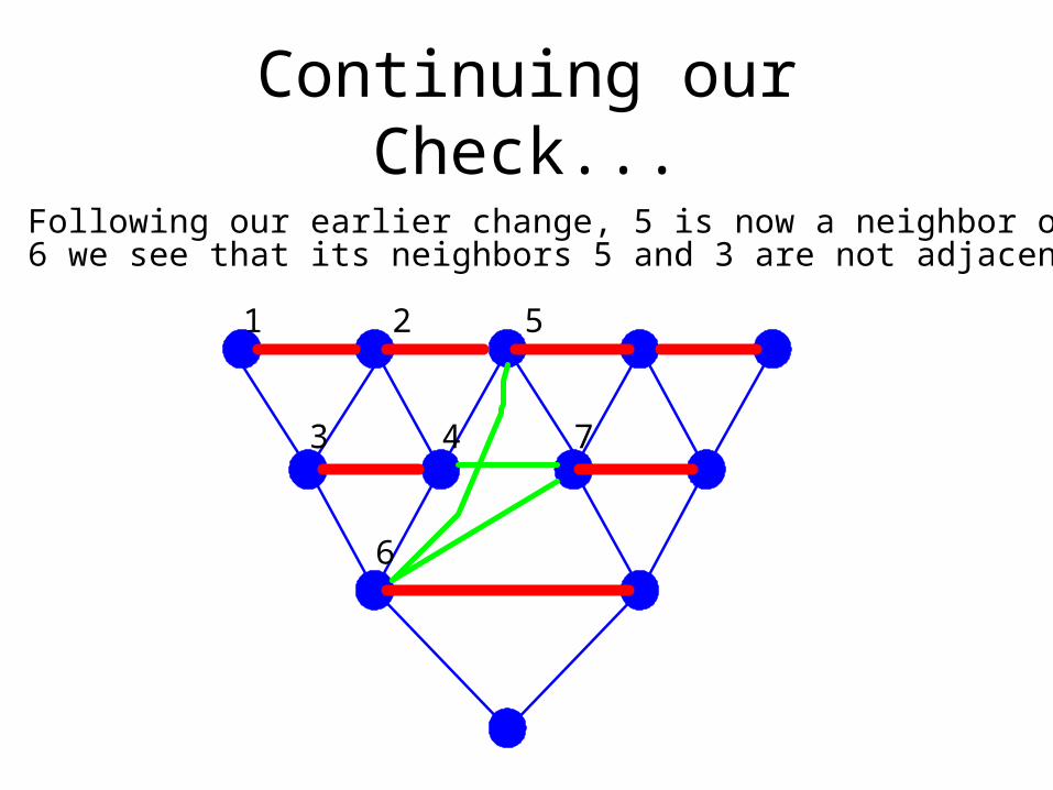
Continuing our Check...
Following our earlier change, 5 is now a neighbor of 6. When we reach
1 2
3 4
5
6
7
6 we see that its neighbors 5 and 3 are not adjacent -- another fix...
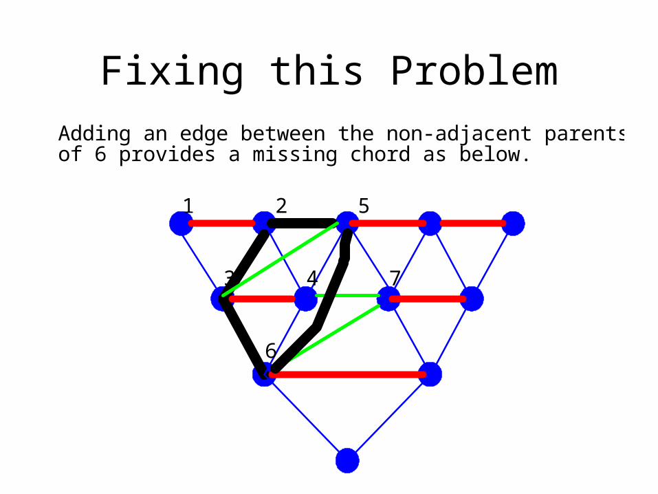
Fixing this Problem
Adding an edge between the non-adjacent parents 3 and 5
1 2
3 4
5
6
7
of 6 provides a missing chord as below.
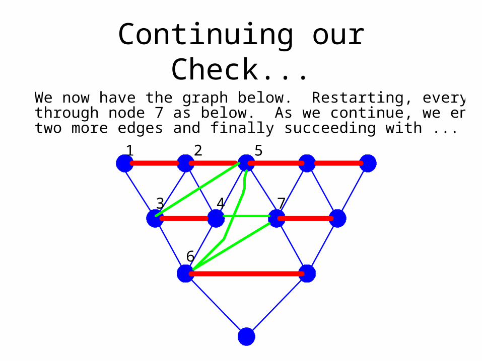
Continuing our Check...
We now have the graph below. Restarting, everything is fine
1 2
3 4
5
6
7
through node 7 as below. As we continue, we end up adding two more edges and finally succeeding with ...
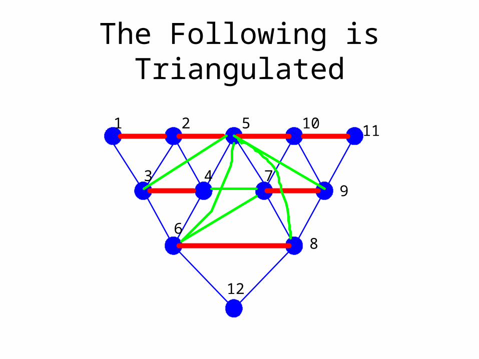
The Following is Triangulated
1 2
3 4
5
6
7
8
9
10 11
12
Triangulation: Key Points
• Previous algorithm is an efficient checker, but not necessarily best way to triangulate.
• In general, many triangulations may exist. The only efficient algorithms are heuristic.
• Jensen and Jensen (1994) showed that any scheme for exact inference (belief updating given evidence) must perform triangulation (perhaps hidden as in Draper 1995).
Definitions
• Complete graph or node set: all nodes are adjacent.
• Clique: maximal complete subgraph.
• Simplicial node: node whose set of neighbors is a complete node set.
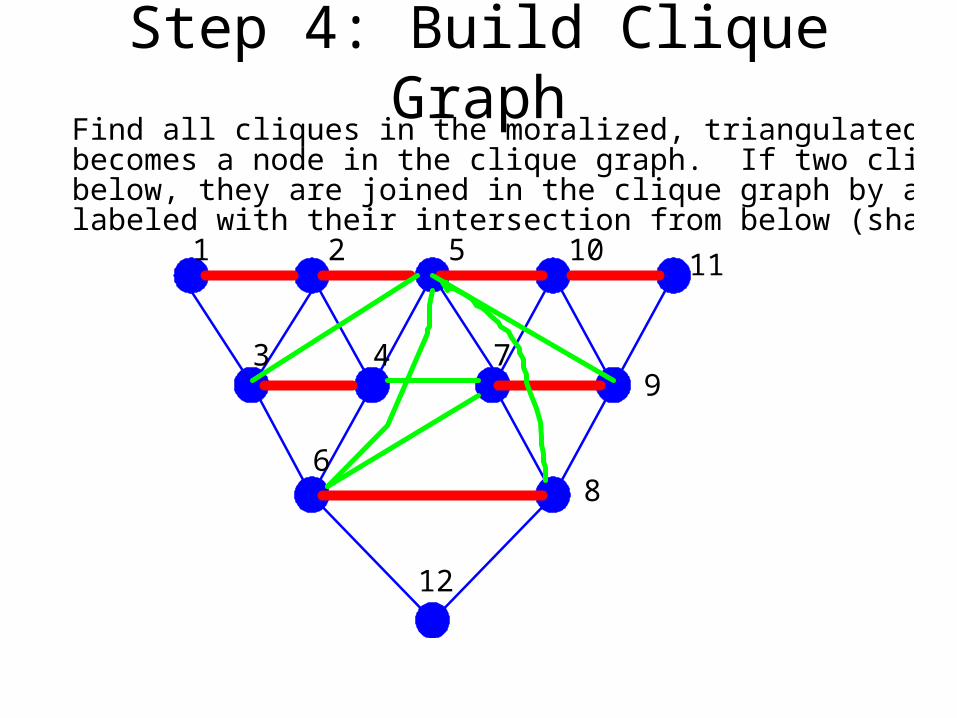
Step 4: Build Clique Graph
1 2
3 4
5
6
7
8
9
10 11
12
Find all cliques in the moralized, triangulated graph. A cliquebecomes a node in the clique graph. If two cliques intersect below, they are joined in the clique graph by an edgelabeled with their intersection from below (shared nodes).
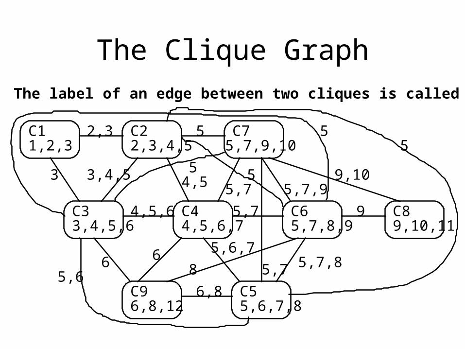
The Clique Graph
C11,2,3
C22,3,4,5
C75,7,9,10
C33,4,5,6
C44,5,6,7
C89,10,11
C96,8,12
C55,6,7,8
C65,7,8,9
2,3
3 3,4,5
5
4,5
4,5,6
5,79,10
9
5,7,9
5,7
6 68
5,6,7
6,8
5,7,8
The label of an edge between two cliques is called the separator.
5,6
5 5
5,7
55
Junction Trees
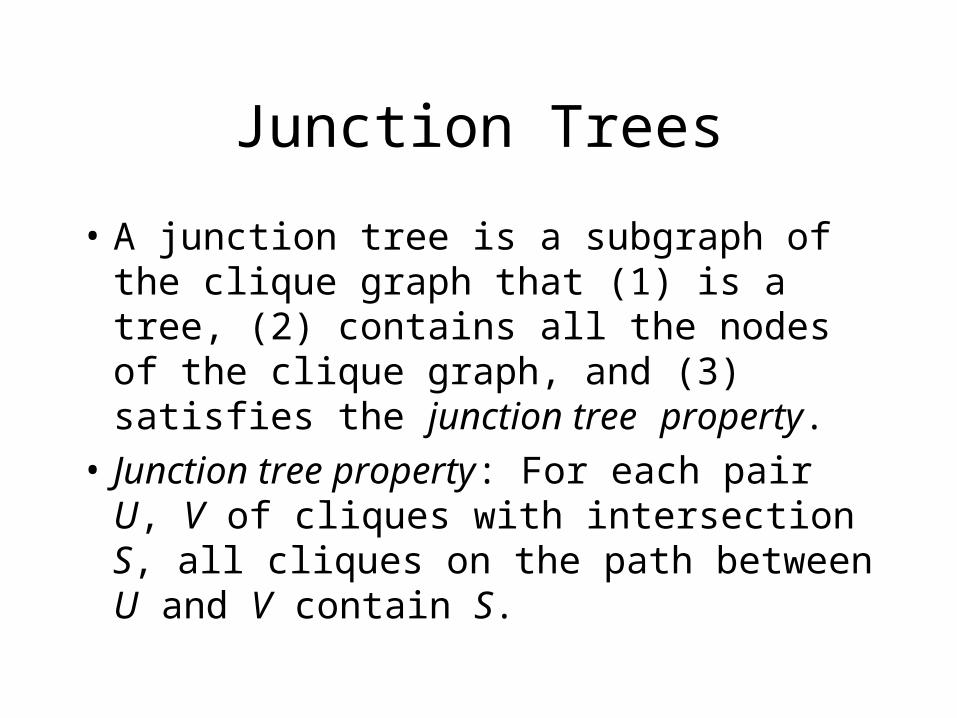
• A junction tree is a subgraph of the clique graph that (1) is a tree, (2) contains all the nodes of the clique graph, and (3) satisfies the junction tree property.
• Junction tree property: For each pair U, V of cliques with intersection S, all cliques on the path between U and V contain S.
Clique Graph to Junction Tree
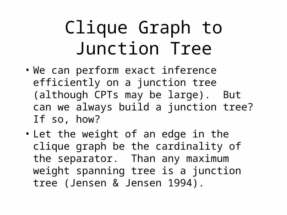
• We can perform exact inference efficiently on a junction tree (although CPTs may be large). But can we always build a junction tree? If so, how?
• Let the weight of an edge in the clique graph be the cardinality of the separator. Than any maximum weight spanning tree is a junction tree (Jensen & Jensen 1994).
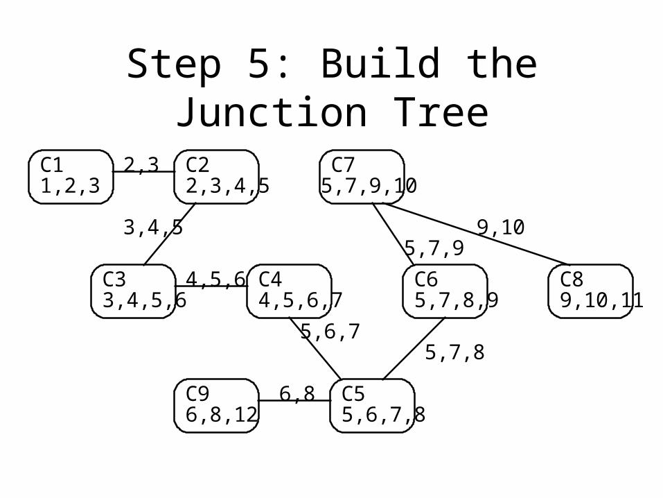
Step 5: Build the Junction Tree
C11,2,3
C22,3,4,5
C75,7,9,10
C33,4,5,6
C44,5,6,7
C89,10,11
C96,8,12
C55,6,7,8
C65,7,8,9
2,3
3,4,5
4,5,6
9,105,7,9
5,6,7
6,8
5,7,8
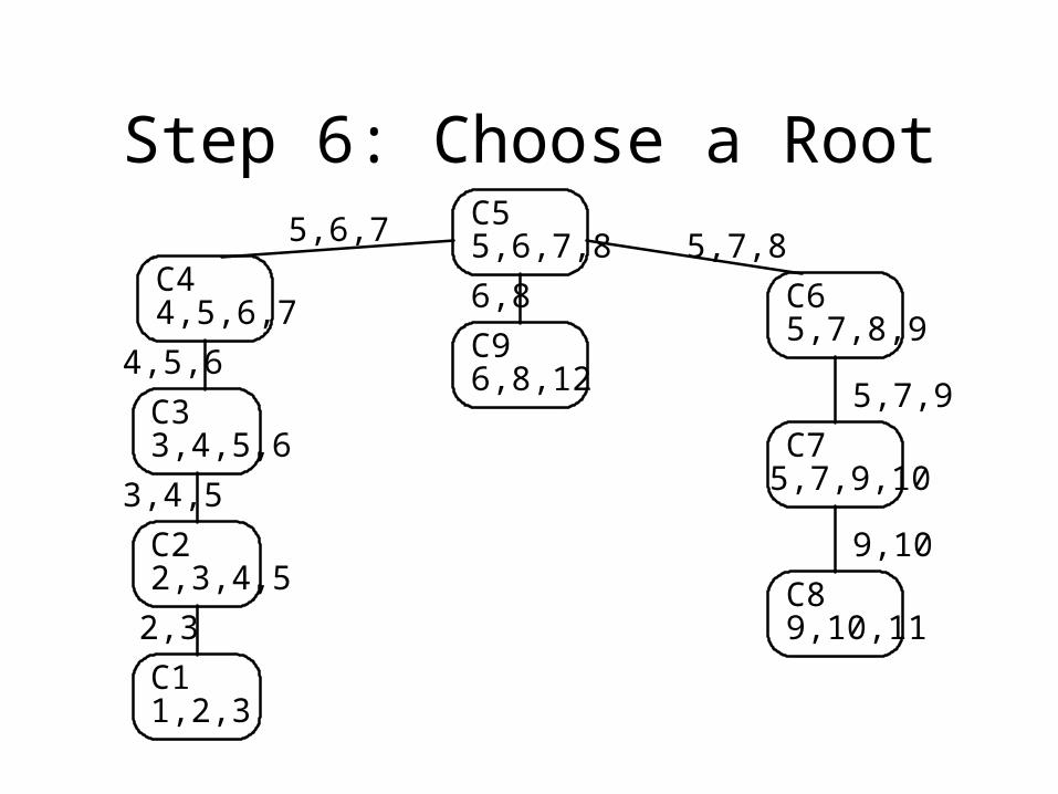
Step 6: Choose a Root
C75,7,9,10
C44,5,6,7
C89,10,11
C65,7,8,9
C11,2,3
C22,3,4,5
C33,4,5,6
3,4,5
2,3
C96,8,12
C55,6,7,8
6,8
5,6,7 5,7,8
4,5,65,7,9
9,10
Step 7: Populate Clique Nodes
• For each distribution (CPT) in the original Bayes Net, put this distribution into one of the clique nodes that contains all the variables referenced by the CPT. (At least one such node must exist because of the moralization step).
• For each clique node, take the product of the distributions (as in variable elimination).
Better Triangulation Algorithm Specifically for Bayes Nets,
Based on Variable Elimination
• Repeat until no nodes remain:– If the graph has a simplicial node, eliminate it (consider
it “processed” and remove it together with all its edges).
– Otherwise, find the node whose elimination would give the smallest potential possible. Eliminate that node, and note the need for a “fill-in” edge between any two non-adjacent nodes in the resulting potential.
• Add the “fill-in” edges to the original graph.
Find Cliques while Triangulating(or in triangulated graph)
• While executing the previous algorithm: for each simplicial node, record that node with all its neighbors as a possible clique. (Then remove that node and its edges as before.)
• After recording all possible cliques, throw out any one that is a subset of another.
• The remaining sets are the cliques in the triangulated graph.
• O(n3), guaranteed correct only if graph is triangulated.
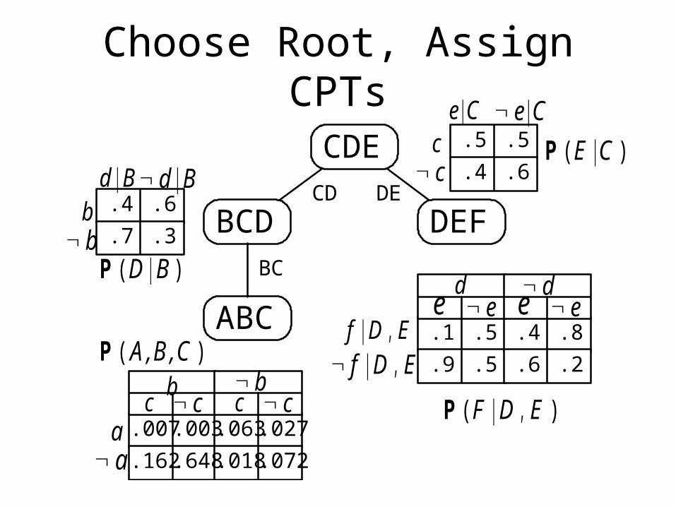
Choose Root, Assign CPTs
DEFBCD.7 .3
.6.4
.5 .5
.4 .6
.1 .5
.5.9 .6 .2
.4 .8ABC
CDE
.007.003
.648.162 .018.072
.063.027
CD DE
BC
a a
d B|d B|b
b
e C| e C|c
c
de e e e
d
f D E| , f D E| ,
b bcc c c
P ( )A ,B ,C
P ( )E C|
P ( )D B|
P ( )F D E| ,
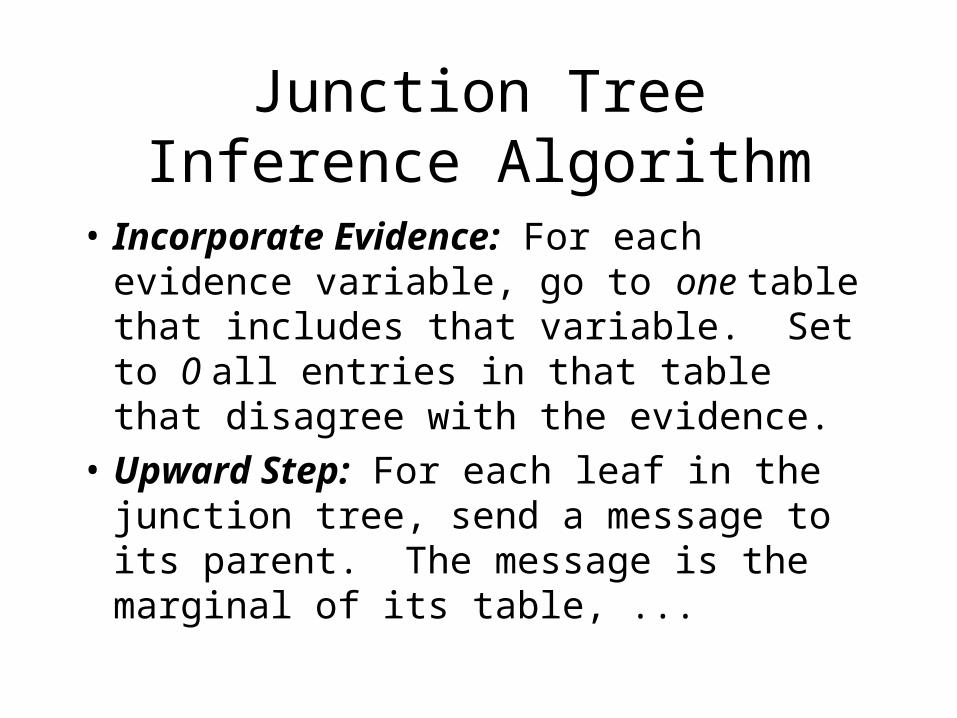
Junction Tree Inference Algorithm
• Incorporate Evidence: For each evidence variable, go to one table that includes that variable. Set to 0 all entries in that table that disagree with the evidence.
• Upward Step: For each leaf in the junction tree, send a message to its parent. The message is the marginal of its table, ...
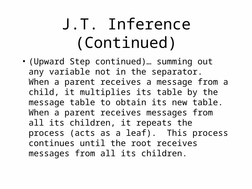
J.T. Inference (Continued)
• (Upward Step continued)… summing out any variable not in the separator. When a parent receives a message from a child, it multiplies its table by the message table to obtain its new table. When a parent receives messages from all its children, it repeats the process (acts as a leaf). This process continues until the root receives messages from all its children.
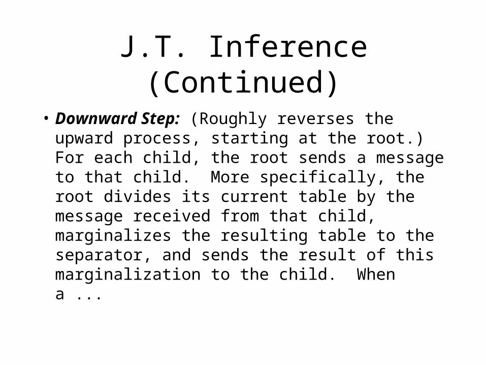
J.T. Inference (Continued)
• Downward Step: (Roughly reverses the upward process, starting at the root.) For each child, the root sends a message to that child. More specifically, the root divides its current table by the message received from that child, marginalizes the resulting table to the separator, and sends the result of this marginalization to the child. When a ...
J.T. Inference (Continued)
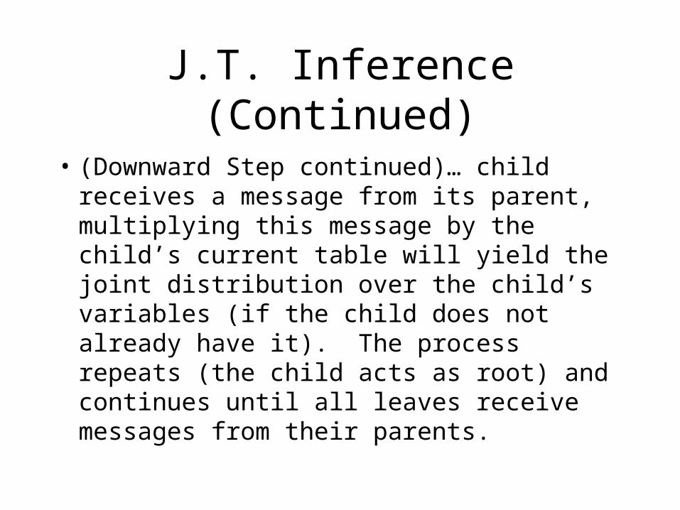
• (Downward Step continued)… child receives a message from its parent, multiplying this message by the child’s current table will yield the joint distribution over the child’s variables (if the child does not already have it). The process repeats (the child acts as root) and continues until all leaves receive messages from their parents.


One Catch for Division
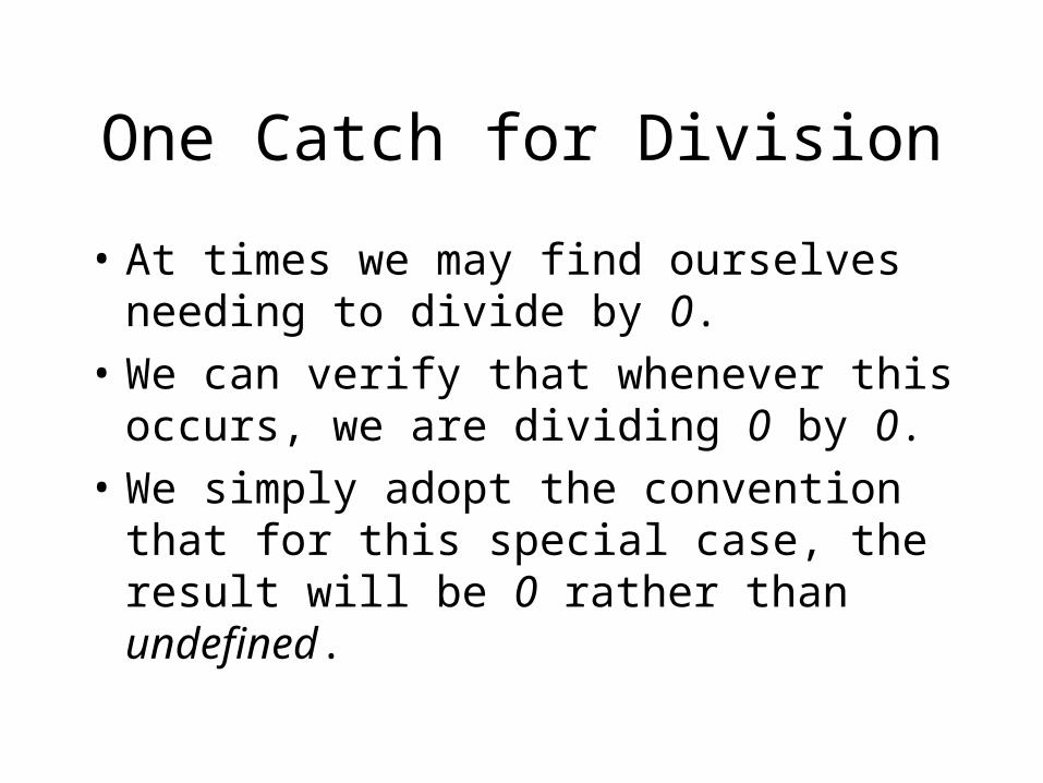
• At times we may find ourselves needing to divide by 0.
• We can verify that whenever this occurs, we are dividing 0 by 0.
• We simply adopt the convention that for this special case, the result will be 0 rather than undefined.
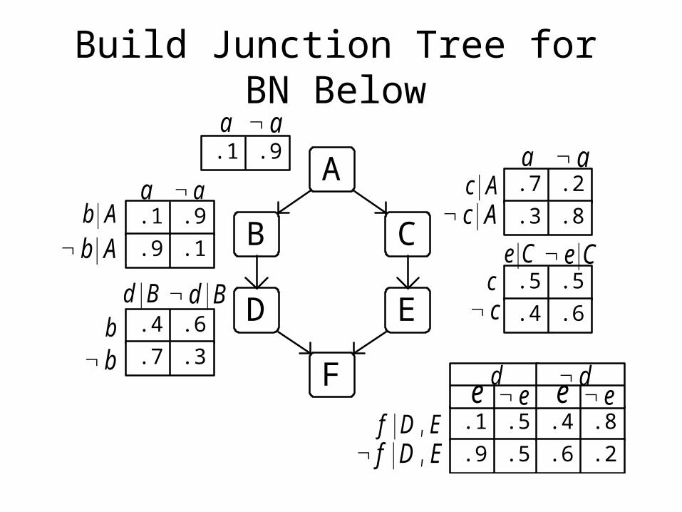
Build Junction Tree for BN Below
A
D E
F
CB
.1 .9
.9
.9
.1
.1
.7
.3 .8
.2
.7 .3
.4 .6
.5 .5
.4 .6
.1 .5
.5.9 .6 .2
.4 .8
a
a
a
ab A|
b A|
a ac A|
c A|
d B|d B|b
b
e C| e C|c
c
de e e e
d
f D E| , f D E| ,
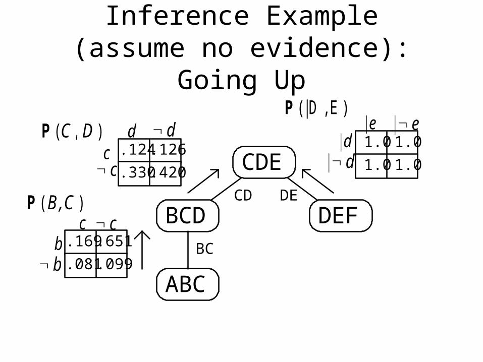
Inference Example (assume no evidence): Going Up
.081.099
.651.169
1.0 1.0
1.0 1.0
DEFBCD
ABC
CDECD DE
BC
.330
.124.126
.420
ddc
c
|e | e|d
| d
b b
c cP ( )B ,C
P ( D , E )|P ( )C D,
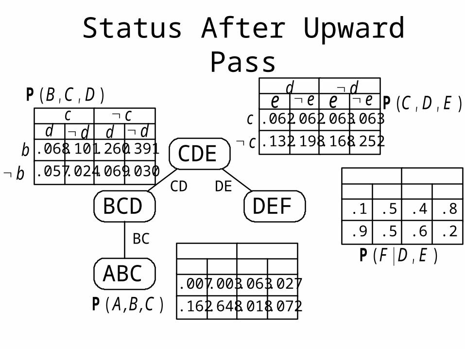
Status After Upward Pass
.1 .5
.5.9 .6 .2
.4 .8
.007.003
.648.162 .018.072
.063.027
DEFBCD
ABC
CDECD DE
BC
.068.101
.024.057 .069.030
.260.391
.062.062
.198.132 .168.252
.063.063
b b
c d
e e
P ( )A ,B ,C
P ( )C D E, ,P ( )B C D, ,
P ( )F D E| ,
ed c
e
ddc
c
d d
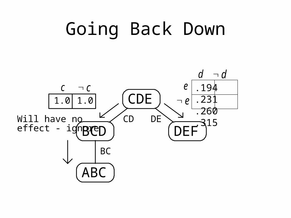
Going Back Down
.194.260
.231.315
DEFBCD
ABC
CDECD DE
BC
1.0 1.0
Will have noeffect - ignore
dde
ec c .194 .231
.260 .315
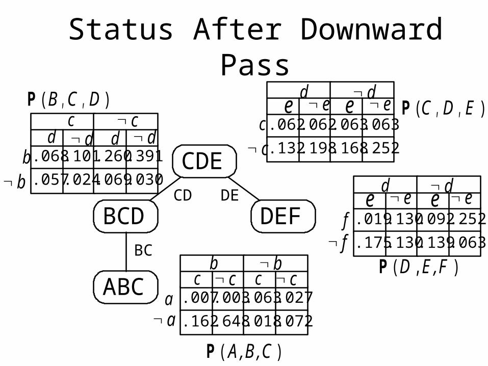
Status After Downward Pass
.019.130
.130.175 .139.063
.092.252
.007.003
.648.162 .018.072
.063.027
DEFBCD
ABC
CDECD DE
BC
.068.101
.024.057 .069.030
.260.391
.062.062
.198.132 .168.252
.063.063
b b
c d
e e
P ( )A ,B ,C
P ( )C D E, ,P ( )B C D, ,
P ( , )D E ,F
ed c
e
ddc
c
d d
d dee e e
f f
b bc c c c
a a
Answering Queries: Final Step
• Having built the junction tree, we now can ask about any variable. We find the clique node containing that variable and sum out the other variables to obtain our answer.
• If given new evidence, we must repeat the Upward-Downward process.
• A junction tree can be thought of as storing the subjoints computed during elimination.
Significance of Junction Trees
• “…only well-understood, efficient, provably correct method for concurrently computing multiple queries (AI Mag’99).”
• As a result, they are the most widely-used and well-known method of inference in Bayes Nets, although…
• Junction trees soon may be overtaken by approximate inference using MCMC.
The Link Between Junction Trees and Variable Elimination
• To eliminate a variable at any step, we combine all remaining distributions (tables) indexed on (involving) that variable.
• A node in the junction tree corresponds to the variables in one of the tables created during variable elimination (the other variables required to remove a variable).
• An arc in the junction tree shows the flow of data in the elimination computation.
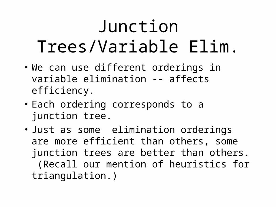
Junction Trees/Variable Elim.
• We can use different orderings in variable elimination -- affects efficiency.
• Each ordering corresponds to a junction tree.
• Just as some elimination orderings are more efficient than others, some junction trees are better than others. (Recall our mention of heuristics for triangulation.)
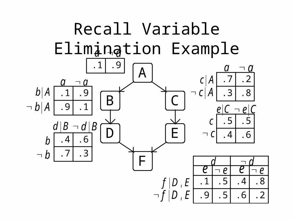
Recall Variable Elimination Example
A
D E
F
CB
.1 .9
.9
.9
.1
.1
.7
.3 .8
.2
.7 .3
.4 .6
.5 .5
.4 .6
.1 .5
.5.9 .6 .2
.4 .8
a
a
a
ab A|
b A|
a ac A|
c A|
d B|d B|b
b
e C| e C|c
c
de e e e
d
f D E| , f D E| ,
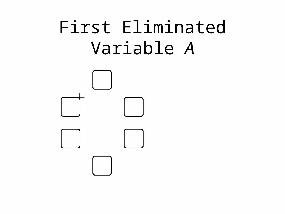
First Eliminated Variable A
A
D E
F
CB.007.003
.648.162 .018.072
.063.027
.169.651
.081.099
a a
b bc c c c
b b
c c
A
P P P P( ) = ( ) ( ) ( )A ,B ,C B |A C |A A
P ( )B ,C
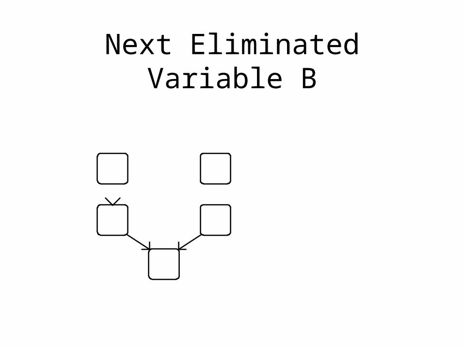
Next Eliminated Variable B
D E
F
CB.068.101
.024.057 .069.030
.260.391
.124.126
.330.420
b b
c dd
c
d dB
dd
c c
P P P( ) = ( ) ( )B ,C ,D D |B B ,C
P ( )C ,D
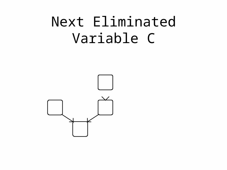
Next Eliminated Variable C
D E
F
C.062.062
.198.132 .168.252
.063.063
.194.260
.231.315
c c
d ee
d
e eC
ee
d d
P P P( ) = ( ) ( )C ,D ,E E |C C ,D
P ( )D E,
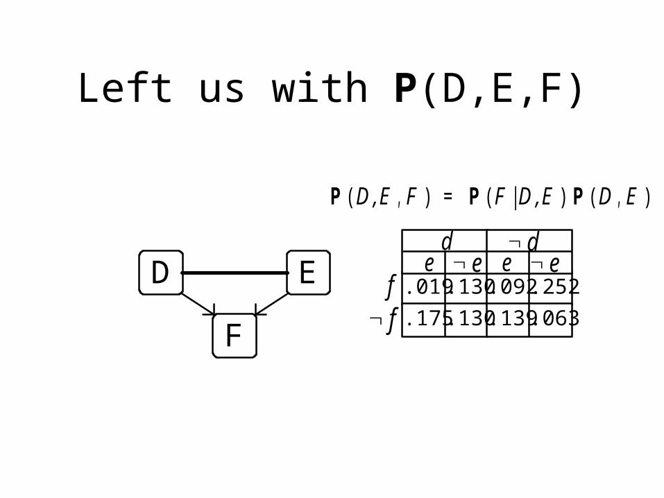
Left us with P(D,E,F)
D E
F
.019.130
.130.175 .139.063
.092.252f f
d ee
d ee
P P P( ) = ( | ) ( )D ,E F F D ,E D E, ,
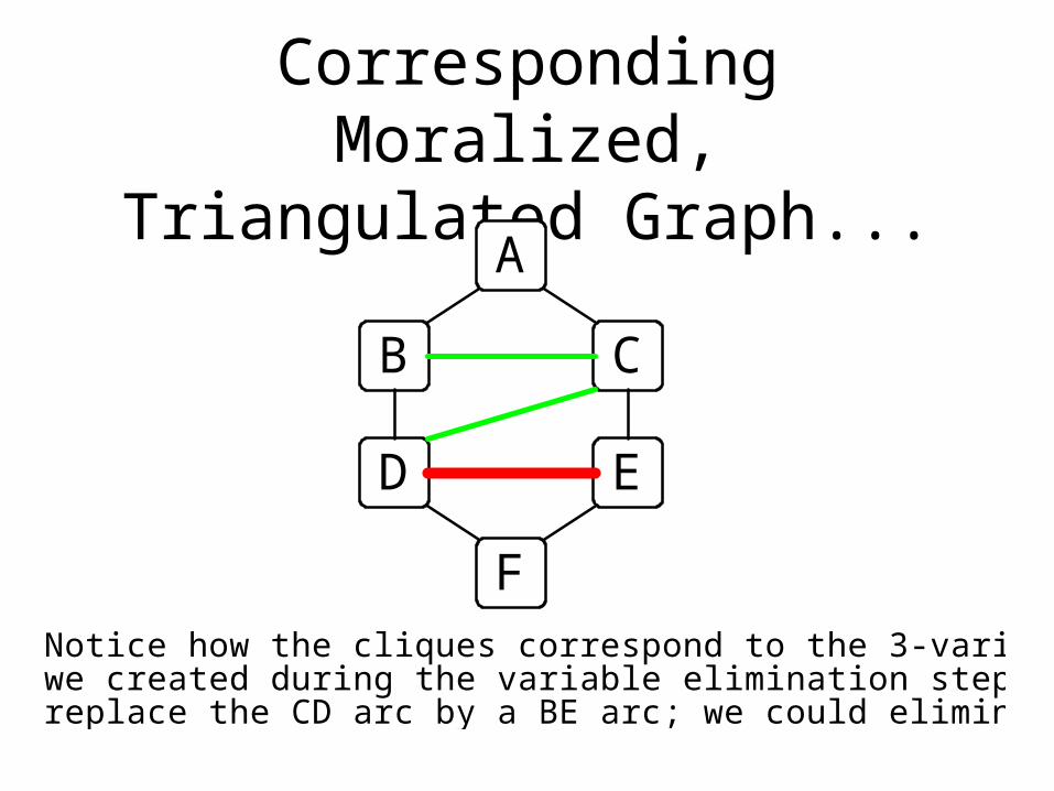
Corresponding Moralized, Triangulated Graph...
A
D E
F
CB
Notice how the cliques correspond to the 3-variable joint tables we created during the variable elimination steps. We couldreplace the CD arc by a BE arc; we could eliminate C before B.