Jumping off of the Great Gatsby Curve: How Institutions

Facilitate Entrepreneurship and Intergenerational Mobility

Journal of Institutional Economics 10(2), 2014: pp. 231-255

DOI: http://dx.doi.org/10.1017/S1744137414000034

Christopher J. Boudreaux

The Florida State University

Abstract:

Income inequality is often attributed to declines in income mobility following

the Great Gatsby Curve, but this relationship is of secondary importance in

determining the factors of income mobility if one considers that changing rules

is more important than changing outcomes under defined rules. Rather,

improvements in institutional quality are hypothesized to increase income

mobility by allowing entrepreneurs the freedom to pursue their dreams. This

paper is the first empirically analyze the institutional determinants behind

entrepreneurship, and their effect on income mobility. The findings from a

cross country analysis suggest that secure property rights and less corruption

are associated with less income persistence leading to higher income mobility,

independent of the Great Gatsby Effect. This suggests that reducing corruption

and the protection of property rights increases income mobility through the

channels of entrepreneurship.

1

I. Introduction

It has been argued that inequality distorts democracy by providing a false sense of the

very idea at the heart of America: If you work hard and you really try, you can make something

of yourself (Wehner & Beschel, 2012). Inequality presents a choice to society: restore an

economy where everyone gets a fair shot, does a fair share, and plays by the same set of rules or

else settle for a country where a smaller number of people do really well and a growing number

of people barely make ends meet. However, while this discussion refers to the pitfalls of income

inequality, income mobility is truly at the center of the issue.

Income inequality only provides an idea of how stratified one country is based on

income. It might be true that a country has a large degree of income inequality, but this does not

mean that the individuals in the lowest income brackets are not becoming better off. Former

president John F. Kennedy once said, "A rising tide lifts all boats but some are raised higher than

others." This adage suggests income inequality is not the real problem. If economic growth raises

income inequality but raises some more than others, then inequality should be of virtually little

importance unless individuals express concerns of equity itself. However, this is not to say that

societies do not benefit from a more equitable income distribution; citizens may value equality of

individuals and not just the well-being of all individuals. Rawls' theory of principle of difference

captures this sentiment. According to his theory, individuals behind a veil of ignorance will

choose societal rules that will provide equal opportunity and maximize the utility of the worst

individual (Rawls, 1971). However, any policy recommendation short of raising substantial

marginal tax rates on individuals with higher income would not make the poor in a society better

off, but instead make the rich worse off. This accomplishes little to help a society. On the other

hand, policies that allow the poor to become better off should not only reduce income inequality

2

but also increase the well-being of the poorest individuals (Wehner & Beschel, 2012). Stated

alternatively, changing the rules of the game (North, 1991) to permit the poorest in society the

equal opportunity to improve their situation is the best policy a society can consider. Buchanan

& Tullock (1962) suggest economists have two choices: they can analyze either a change in

outcomes within a set of narrowly defined rules (Hayek, 1960) or a change in the rules

themselves.

Cross country studies have provided some evidence of association between inequality

and corruption (Gupta et al., 2002), economic freedom (Berggren, 1999), per capita income (Ku

& Salmon, 2012) and many others. Even if there turns out to be no relationship between income

inequality and per capita income (Barro, 2000), income inequality remains an important

launching pad for the institution of income mobility.

Income mobility addresses this idea of the possibility or the potential of an individual to

move from one income bracket to another. Typically, individuals are grouped into five brackets

known as quintiles. The idea of income mobility then can be analyzed by looking at the

likelihood of an individual of moving from one income bracket into another. While individuals

can move between any income brackets, the interesting case is how likely an individual is to

move out of a lower quintile and into a higher one during his lifetime. This idea can be measured

two ways: the first method is to look at the income of an individual when he is young and then

look at that same individual’s income later on in life when he is older. Then one can compare to

see if his income has increased, and more importantly if he has changed income quintiles. This is

known as intragenerational mobility. The alternative is to compare the income information for

an individual and his parent.

3

The idea behind this method is that parents who are better off economically will invest

more in their children’s futures. Parents who derive more utility from raising successful offspring

tend to endow their children with a greater variety of investment and consumption opportunities.

As a consequence, children whose parents invest more in their future will be better off

economically. As Becker & Tomes (1979) point out, the endowment of children's attributes, "are

determined by the reputation and connections of their families, and the learning, skills, goals, and

other family commodities acquired through belonging to a particular family culture." This latter

measure is known as intergenerational mobility or the "rise and fall of families" (Becker &

Tomes, 1986). This method is much more commonly used for research. Empirical estimates of

intergenerational mobility are known as intergenerational earnings elasticities, and these are

measured as follows:

(1)

where Yi,t is the logarithmic income of a descendent, Yi,s is the log wage of the parents, and εi,t is

a white-noise error term. The coefficient, β, is the measure of the intergenerational income

elasticity (Solon, 1992; Zimmerman 1992; Altzinger & Schnetzer, 2013).

Andrews & Leigh (2009) specify criteria for which good measures can be taken for

income mobility. Ideally, they claim this data should come from comparable sources to capture

cross-country differences. This way one would receive meaningful results and not just results

stemming from the differences in the data construction. Also, they mention that the data should

come from estimates based on fathers and sons during economically active ages. Therefore, the

first strategy in this article will be to analyze the sub sample of intergenerational elasticity

estimates from Corak (2012). These estimates possess the smallest measurement error since they

are derived from fathers and sons in a comparable manner. Analyzing these cross country

4

observations provides the best chance that differences in outcomes are not due to differences in

data construction. First, qualitative results are drawn from scatter plots using the smaller sub-

sample. Second, quantitative results are derived from Ordinary Least Squares (OLS) using the

entire sample of cross country observations sample of intergenerational elasticity estimates from

Corak (2012).

The paper will proceed in the following manner: Section II is a review of the literature.

Section III discusses the data and methodology. Section IV discusses the quantitative and

qualitative strategies involved in analyzing the relationship between institutions that facilitate

entrepreneurship and income mobility. Section V discusses the results while section VI closes

with concluding remarks and suggestions for further research.

II. Literature Review

Corak (2012) looks at the intergenerational earnings elasticity between the United States

and twenty-four other countries, and he uses the most common method of analyzing the

intergenerational earnings elasticity between fathers and sons (Corak, 2012). For a recent review

of the literature on intergenerational income mobility see Corak (2013). Sometimes data is drawn

from mothers and sons, fathers and daughters, mothers and daughters, and some combination of

parents and children (Schnetzer &Altzinger, 2013). Schnetzer & Altzinger (2013) only refer to

their estimate of the intergenerational earnings elasticity for Austria as parents to children.

Furthermore, concerns might arise due to different studies using data from different years of

cohorts. Data for intergenerational income mobility is derived from two surveys for the United

States: the Panel Study of Income Dynamics (PSID) and the National Longitudinal Surveys

(NLS) of labor market experience (Solon, 2002).

5

Andrews & Leigh (2009) examine the relationship between income inequality and

mobility. They find evidence to suggest that there is indeed a negative association between

inequality and mobility. That is, more income inequality is correlated with less income mobility;

sons who grew up in countries that were more unequal in the 1970s had a worse chance for

increased social mobility in the late 1990s.

Corak (2012) analyzes the relationship between income inequality and mobility and calls

this the “Great Gatsby Curve.” Income inequality is captured by the Gini coefficient and is

measured on the horizontal axis. Income mobility is captured by the intergenerational income

elasticity measures and is displayed on the vertical axis. Gini coefficients are measured between

0 and 100 where zero means complete income equality and 100 means complete income

inequality. The intergenerational income elasticity, β, measures the persistence of income from

one generation to the next. That is, it measures how likely one individual is to follow in a

parent’s footsteps in relation to the income distribution. Thus, a lower β means an individual has

lower earnings persistence and therefore higher income mobility. The positive trend line on the

Great Gatsby Curve illustrates an inverse relationship between income inequality and income

mobility; countries with more income inequality have greater earnings persistence between

generations and less income mobility.

The Great Gatsby Curve (Corak, 2012) has certain policy recommendations. If the

relationship is such that the higher inequality in a country, the lower the mobility, then policies

for higher social mobility are recommended to be accompanied by policies for more equal

societies. In a policy recommendation, OECD (2010) suggests progressive tax systems and social

transfer programs should not only make a society more equal but also strengthen the chances for

6

individual social and economic advancement. Alternatively, economic regulations and

ineffective government may explain declines in income mobility.

Policies consistent with improvements in economic institutions are hypothesized to allow

for greater income mobility. If citizens are free to engage in commerce with others and if they do

not fear their property will be stolen from them, then they should face better opportunities to

experience the American Dream through income mobility. Specifically, regulatory constraints

should have a large impact on income mobility. Indeed, this has been offered as an explanation

of why income mobility (inequality) has decreased (increased) in the United States in the past

few decades (Clark & Lawson, 2008).

In his inquiry on the mystery of capital, De Soto (2000) finds that capitalism succeeds in

the west, and fails everywhere else. One contributing factor is that the barriers to

entrepreneurship and acquiring private property are so tedious that citizens cannot improve their

economic well-being. De Soto's team of researchers found that it took them 289 days to register a

legal business enterprise in Peru while working at it for six hours a day filling out forms,

standing in lines, and acquiring certifications necessary to operate. In total, the cost of legal

registration was $1,231, which was 31 times the monthly minimum wage. Similarly, in the

Philippines, the process to registering private property required 168 steps, involving 53 private

and public agencies, and taking anywhere from 13 to 25 years. They also found it would take

someone 5 to 14 years in Egypt and 2 years in Haiti (De Soto 2000, p. 20-21). Therefore, it

follows that sound economic institutions for commerce and entrepreneurship matter; sound rules

allow individuals to prosper, and this is hypothesized to be reflected in greater income mobility.

III. Data & Methodology

7

Data on political and economic institutions is available to test the hypothesis that fewer

burdens and regulations allow for more income mobility. There are six World Wide Governance

Indicators (WGI) from Kauffman et al. (2011): government effectiveness, control of corruption,

voice and accountability, regulatory environment, rule of law, political stability and absence of

violence and terrorism. Since entrepreneurship is hypothesized to influence income mobility,

only three of these variables are used to ascertain whether burdens and regulations stymie

income mobility; (i) government effectiveness, (ii) regulatory quality, and (iii) the rule of law.

According to the WGI, government effectiveness "reflects perceptions of the quality of public

services, the quality of the civil service and the degree of its independence from political

pressures, the quality of policy formulation and implementation, and the credibility of the

government's commitment to such policies." Regulatory quality "reflects perceptions of the

ability of the government to formulate and implement sound policies and regulations that permit

and promote private sector development." Rule of law "reflects perceptions of the extent to

which agents have confidence in and abide by the rules of society, and in particular the quality of

contract enforcement, property rights, the police, and the courts, as well as the likelihood of

crime and violence" (Kauffman et al. 2011). All three of these explanatory variables range from -

2.5 to 2.5 where 2.5 indicates a country has a more productive regulatory environment, an

effective quality of government, and a judicial and legal system that protects property rights.

These three measures are then interpreted as follows: higher political, economic, and judicial

quality of institutions as measured by the WGI are associated with higher numbers on the scale

of -2.5 to 2.5.

Transparency International collects annual data on corruption known as the corruption

perceptions index (CPI). It measures the perceived levels of public sector corruption in 176

8

countries and territories around the world by utilizing surveys from multiple, comparable

sources, and it aggregates the results to construct the CPI index. The data are measured on a

scale of 1 to 10 where 1 has very little corruption and 10 is the most corrupt. The CPI index by

Transparency International was chosen for the analysis rather than the World Bank's control of

corruption measure because the latter is another measure under the World Governance Indicator

similar to government effectiveness and regulatory quality. Multiple sources and alternative

institutional measures will do a better job of ascertaining the effects of institutional quality on

income mobility.

To the best of my knowledge, there are currently 32 countries with an available β

coefficient, the measure of intergenerational earnings elasticity derived from equation (1).

Twenty-five of these estimates are available from Corak (2012). The other seven come from

other studies. In total there are 15 studies with at least one estimate of the intergenerational

earnings elasticity for a country. These studies and their β coefficients are listed in Table 1.

While there are some countries with only one β coefficient from one study, there are also quite a

few countries with multiple β coefficients from multiple studies. For the empirical estimates

derived in this study, intergenerational earnings elasticity estimates are taken from Corak (2012)

which provides β coefficients for 25 countries. The other studies have been listed in Table 1 in

hopes that the data from these studies are useful to other researchers, but their estimates are not

included in the scatter plots, correlation coefficients, and Ordinary Least Squares (OLS)

regressions. The other intergenerational earnings elasticity estimates are not included in an

attempt to minimize measurement error because they may use other combinations of cohorts

such as: fathers and daughters, mothers and sons, and different time spans of study. Thus,

empirical estimates derived from sources other than Corak (2012) may actually capture

9

differences in data collection rather than cross country differences in income mobility. A more

concerning issue is with the accuracy of the parental income available from the NCDS.

Zimmerman (1992) has critiqued the increase in income mobility as a result of measurement

error arising from attenuation bias in the NCDS. The results here are reported using income data

from the NCDS, and it cannot be ruled out that attenuation bias is not present. However, Blanden

et al (2013) argue that their findings run counter to these claims because they stem from

observable characteristics, which are free from the influence of attenuation bias. Therefore, this

provides some evidence that increases in income mobility may arise for reasons other than

attenuation bias.

[Insert Table 1 About Here]

The gini coefficient is another explanatory variable used to capture the Great Gatsby

effect, and it is taken from Deininger & Squire (1996). This gini is subject to a couple of

criticisms (Atkinson & Brandolini, 2001; Galbraith & Kum, 2005). Most notably, the gini for

China is lower than in Europe, which is a striking result. However, the results presented here are

robust to the substitution of the gini measure used by the World Bank.1 The distance to the

equator is also included as an additional measure of economic institutional quality (Hall & Jones,

1999). It is hypothesized that countries located farther away from the equator set up better

economic institutions.2

The Great Gatsby Curve and the relationship between institutional measures and income

mobility are depicted in Figure 1 below. The correlation coefficient of income inequality and the

intergenerational earnings elasticity is 0.47, which is the lowest correlation coefficient among all

five measures. In addition, there are four institutional measures hypothesized to be associated

10

with income mobility: (i) government effectiveness, (ii) regulatory quality, (iii) rule of law, and

(iv) corruption.

[Insert Figure 1 About Here]

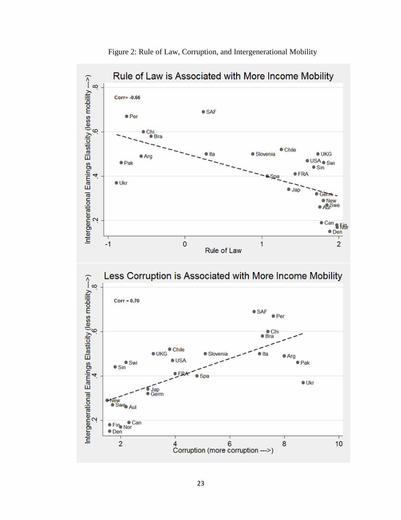
Rule of law is located at the top of Figure 2, and it has a correlation coefficient of -0.66.

This suggests that the security of property rights is positively correlated with income mobility as

measured by intergenerational earnings elasticity. The relationship between corruption and

income mobility is depicted at the bottom of Figure 2. This relationship boasts the highest

correlation coefficient of 0.70; more corruption is associated with higher earnings persistence

and lower income mobility.

[Insert Figure 2 About Here]

Regulatory quality, is depicted at the top of Figure 3, and the correlation coefficient is -

0.52, which suggests a lower regulatory burden is associated with lower earnings persistence and

higher income mobility. Finally, government effectiveness is located at the bottom of Figure 3,

and its correlation coefficient with income mobility is -0.62; an effective government is

associated with less income persistence and higher income mobility. All five of these measures

and the correlation coefficients are illustrated in Figure 4 below.

[Insert Figure 3 About Here]

[Insert Figure 4 About Here]

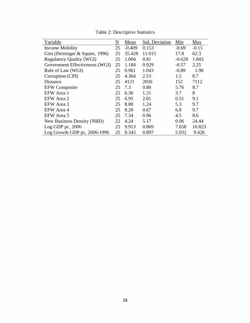
Table 2 illustrates the descriptive statistics for the variables used in this study. The

dependent variable is a measure of income mobility using collected data on intergenerational

income elasticity measures. Values for the intergenerational earnings elasticity range from -0.15

to -0.69 which correspond to Denmark and South Africa, respectively. Typically, these values

are positive as shown in Table 1 and Figure 1, but in order to make the results easier to interpret,

11

the signs have been flipped for the intergenerational earnings elasticity measure in the regression

output. The way to interpret the income mobility measure is simple; it measures the degree of

earnings persistence from one generation to the next. Higher values for the intergenerational

income elasticity translate into more persistence in earnings and consequently less income

mobility. Since smaller values mean more income mobility, it makes more sense to make them

negative. This would allow larger numbers to express more income mobility as it is easier to

interpret. Thus, income mobility measures are multiplied by negative unity.

The gini coefficient is measured on a scale of 0 to 100 where 0 means completely equal

wealth and 100 means one person owns all of the wealth. The minimum in the 25 country data is

17.8 and the maximum is 62.3 with a mean gini coefficient of 35.428. The largest gini coefficient

corresponds to South Africa, and the smallest gini coefficient corresponds to China. Data on per

capita income and the growth of per capita income are taken from the Penn World Tables

(Heston et al., 2012).

[Insert Table 2 About Here]

Kirzner (1979) argues that private property rights, free enterprise, and sound money

foster an environment where subconscious learning can occur, and the alert entrepreneur

discovers these profitable opportunities. Excessive regulations which curtail business activity

and consequently make it harder for poorer people to become entrepreneurs are barriers to

increasing income mobility. If this is true, removing some of these barriers, regulations, and red

tape are posited to improve income mobility. This leads to the first hypothesis.

Proposition 1: Institutional quality that allows entrepreneurs the chance to flourish is

associated with greater income mobility.

12

Another alternative has been suggested by OECD (2010). The idea captures the Great

Gatsby relationship. Subsequently, they suggest a policy recommendation of increasing social

transfers which should reduce income inequality and increase income mobility. These social

transfers can be thought of as increased government spending on education and healthcare. It is

hypothesized that education expenditures by the government allows economically disadvantaged

groups the opportunity to increase their earnings capacity by receiving an education. In a study

of US states, Mayer & Lopoo (2008) find that high spending states possess greater income

mobility than low spending states. Similarly, healthcare expenditures help to ensure citizens in

society are healthy and facilitate movement between income brackets for economically

disadvantaged citizens. Several studies support this claim. Case et. al (2005) suggest that a large

share of the intergenerational transmission of socioeconomic status works through the channel of

parents' income to their children's health. Eriksson et. al (2005) report that the intergenerational

earnings elasticity in Denmark falls by 25-28% when controlling for their parental health status.

Hertz (2007) finds that the relationship between parental income and health status explains 8% of

intergenerational correlation of income in the United States. Similarly, poor health explains 5-

10% of the variation in an offspring's income mobility (Esping-Anderson & Wagner, 2010). For

a larger review of the literature, see Nolan et. al (2010).

Proposition 2: Countries with greater spending on education and healthcare should be

associated with greater income mobility.

In order to test these two hypotheses, an empirical specification using Ordinary Least Squares

(OLS) is employed, and the form of the equations estimated is specified as follows:

for i=1…n (2)

13

where the dependent variable, Income Mobility, refers to the intergenerational income

elasticity; X', is a vector of institutional variables that are of interest in explaining the variation in

income mobility, and it includes rule of law, corruption, regulatory quality, and government

effectiveness; δ' is a vector of control variables that may be important in analyzing the

relationship between institutional quality and income mobility. Included in this control vector are

the growth of per capita income, the level of GDP per capita, the gini coefficient, distance to the

equator, government expenditures on education, and government expenditures on healthcare.

IV. Results

The first relationship to empirically measure is the association between income inequality

and intergenerational earnings elasticity. The measure of income inequality, gini coefficient, is

statistically significant in all five specifications under OLS, but it is only marginally significant

(p<.10). Analyzing the marginal effects suggests that increasing a country's income inequality by

10 points on the gini coefficient is associated with a 0.07 increase in intergenerational elasticity,

which is an increase (decrease) in income persistence (income mobility).3 Table 3 These

specifications capture both the effect of gini coefficient on intergenerational earnings elasticity

without institutional controls in column (1) and with alternative institutional controls in columns

(2) through (5). Note that the t-statistics are above the common critical value in large sample

studies. However, due to the small sample size, the critical value has increased from 1.96 to 2.11.

Thus, one can only discern a marginally statistically significant relationship illustrating the Great

Gatsby Effect.

The first institutional measure, corruption, is the only measure that exhibits a statistically

significant relationship (p<0.05) with intergenerational earnings elasticity; the results suggest

14

that corruption is inversely related to income mobility. Analyzing the marginal effect suggests

that a one point increase in corruption as measured by Transparency International's Corruption

Perception Index (CPI) is associated with a 0.04 increase in earnings persistence, which is a

decrease in income mobility. Further, the greatest proportion of the variation in income mobility

is explained by the specification that includes both the gini coefficient and corruption in column

(2) with an adjusted R2 of 0.53.

Column (3) is the only other alternative specification that exhibits a statistically

significant influence on intergenerational earnings elasticity, but the positive relationship

between rule of law and intergenerational earnings elasticity is only marginally significant with a

t-statistic of 1.95. The results suggest that for every one point increase in rule of law there is an

associated 0.086 decrease in income persistence or increase in income mobility.

The remaining two institutional measures exhibit very little statistical influence on

intergenerational earnings elasticity. Further, the social transfer variables such as government

spending on education and healthcare are never statistically significant in any empirical

specification. In addition, there is scant evidence that variations in income alone have any

statistical influence on income mobility. The one exception is in column (1), which excludes any

controls for institutional measures. Income information on the levels of Gross Domestic Product

(GDP) per capita and growth rates of GDP per capita are generally statistically insignificant. The

level of GDP per capita has a positive effect on income mobility, and the growth rates of GDP

per capita have a negative effect on income mobility. The level of GDP per capita in the first and

last specification of Table 3 does possess a positive and statistically significant relationship with

income mobility. The marginal effects suggest that a 1% increase in per capita GDP is associated

with a 0.17-0.19 decrease in the intergenerational elasticity, which is an increase in income

15

mobility. However, these results are fragile to the specifications (2) through (5). Finally, distance

to the equator (Hall & Jones, 1999) exhibits no statistical influence on income mobility.

Baumol (1990) discusses how individuals can either be productive or destructive as

entrepreneurs, contingent on the institutional environment; market institutions that promote

commerce will experience productive environment, and institutions that promote government

intervention and favoritism will largely be destructive. Sobel (2008) finds evidence to confirm

this theory. Following this work, table 4 analyzes the same relationship between institutions

and income mobility, but it also considers a more direct link of entrepreneurship using a measure

of new business density (NBD) taken from the World Bank's Doing Business project. While this

is not a perfect measure of entrepreneurship, it serves as a proxy to the extent that individuals can

start their own business and ventures. A greater number of new businesses suggests that the

market environment is conducive to entrepreneurship. The positive relationship between NBD

and income mobility in Table 4 confirms the a priori expectations; countries that have a greater

number of new businesses tend to also have higher income mobility and lower earnings

persistence, but this relationship erodes when controlling for the institutional framework and

healthcare and education expenditures per person. One interpretation is that institutions matter

for entrepreneurship; it is not the density of new business startups that affect income mobility.

Rather, it is the environment that allows or prohibits entrepreneurship that matters. Another

explanation is that healthcare and education expenditures allow for individuals to start new

business.

The Great Gatsby effect is stronger under the specifications in Table 4 than in the

previous table. While the magnitudes of the coefficient are slightly larger, the real change is that

all specifications exhibit a statistically significant (p<0.05) and inverse relationship between

16

income inequality and income mobility. The relationship between the institutional measures and

income mobility remains largely unchanged in Table 4 from the previous table. Corruption

exhibits an inverse and statistically significant relationship with income mobility, and the rule of

law exhibits a positive association with income mobility. However, the rule of law measure fails

to meet the 5% rejection threshold, which is the same result from Table 3. However, the rule of

law possesses a t-statistic that is very close to rejection at the 5% threshold, and this relationship

deserves a closer examination.

Table 5 looks closer at the relationship between institutions and income mobility using

the composite index of economic freedom, and its individual component areas using the

Economic Freedom of the World Index (EFW) updated annually by Gwartney & Lawson (2012).

The EFW index provides a robustness check, as it is a frequently used measure of the quality of

economic institutions. The EFW index is designed to measure the degree of economic freedom

that exists in a country, and to leave out measures of political freedom, such as civil liberties or

democratic government. The EFW index measures economic freedom by grouping 42

components into five areas: (1) size of government, (2) legal structure and security of property

rights, (3) access to sound money, (4) freedom to trade internationally, and (5) freedom from

regulation. Refer to Berggren (2003) and Faria & Montesinos (2009) for literature reviews of the

EFW index.

Analyzing the individual component areas suggests that the rule of law is positively

associated with income mobility, and it is statistically significant at conventional levels (p<0.05).

The marginal effects suggests that an increase of one in area 2 of the EFW index is correlated

with a 0.028 decrease in income persistence, which is an increase in income mobility. Notice that

the magnitude is smaller using area 2 of the EFW index than the rule of law (WGI). This is

17

because EFW is measured on a scale of 1 to 10, and the World Governance Indicator's rule of

law is scaled from -2.5 to 2.5. The composite EFW index is used under the sixth specification,

and the results suggests a positive relationship between institutional quality and income mobility.

However, this effect is statistically insignificant at conventional levels (p<0.05), and it has a t-

statistic of 2.05, which is just over the threshold. One explanation is that the rule of law, equality

under governance and the protection of property rights, affects income mobility, but the

remaining individual component areas exhibit little to no influence on income mobility. Finally,

notice that income information has been omitted in the first six specifications, and it is included

in the last specification. It has been purposely omitted in order to avoid the multicollinearity

present between economic freedom, income levels, and income growth. The last specification

includes the composite economic freedom measure, the level of GDP per capita, and the growth

of GDP per capita. As expected, economic freedom exhibits very little influence on income

mobility under this specification.

V. Concluding Remarks

This article has provided evidence to suggest improvements in institutional quality can

increase income mobility. Economic theory supports these findings because improvements in

regulations and a less burdensome economy facilitate income mobility. The empirical estimates

in this study suggest that lack of corruption and secure property rights are associated with

reductions in intergenerational earnings persistence, which leads to greater income mobility. In

addition, empirical support is found for the Great Gatsby effect in the data. However,

independent of this effect, the results suggest that the dream of income mobility can be supported

18

through high quality institutions that facilitate entrepreneurship and the protection of property

rights.

The other hypothesis, that social transfer programs such as government spending on

education and healthcare will increase income mobility for a society finds little support, although

other studies do find a relationship between healthcare spending and income mobility (See Nolan

et al, 2010 for a review of this literature). This finding in conjunction with the first suggests that

institutions matter (North, 1991) for income mobility by facilitating the entrepreneurial process.

In order to allow everyone the opportunity to realize the dream of income mobility, countries

must allow sound institutions to foster entrepreneurship. Only then will income mobility persist

as a reality and not merely a dream.

References

Andrews, D. & Leigh, A. (2009). More inequality, less social mobility. Applied Economics

Letters. 16(15), 1489-92.

Atkinson, A. & Brandolini, A. (2001): “Promise and Pitfalls in the Use of Secondary Data-Sets:

Income Inequality in OECD Countries as a Case Study”. Journal of Economic Literature

39(3), 771–799.

Barro, R. (2000). Inequality and Growth in a Panel of Countries. Journal of economic growth,

5(1), 5-32.

Baumol, W., 1990. Entrepreneurship: productive, unproductive and destructive. Journal of

Political Economy 98 (5), 893–921.

Becker, G., & Tomes, N. (1979). An equilibrium theory of the distribution of income and

intergenerational mobility. The Journal of Political Economy, 1153-1189.

Becker, G., & Tomes, N. (1986) "Human Capital and the Rise and Fall of Families." Journal of

Labour Economics, July, (4), 1-39.

Berggren, N. (1999). Economic Freedom and Equality: Friends or Foes? Public Choice.

100, 203-223

Berggren, N. (2003). The benefits of economic freedom: a survey. The Independent

Review, 8(2), 193-212.

Blanden, J., Gregg, P., & Macmillan, L. (2013). Intergenerational persistence in income and

social class: the effect of within-group inequality. Journal of the Royal Statistical Society:

Series A (Statistics in Society), 176(2), 541-563.

Buchanan, J. M., & G. Tullock (1962). The calculus of consent. Ann Arbor, 306.

Carter, J. (2006). An empirical note on economic freedom and income inequality. Public

Choice, 130(1-2), 163-177.

Case, A., Angela F., & Paxson, C. (2005). The lasting impact of childhood

19

health and circumstances. Journal of Health Economics, 24: 365-389.

Clark, J., & Lawson, R. (2008). The impact of economic growth, tax policy, and economic

freedom on income inequality. Journal of Private Enterprise, 24(1), 23-31.

Corak, M. (2006). Do poor children become poor adults? Lessons from a cross country

comparison of generational earnings mobility, IZA Discussion Papers, No. 1993.

Corak, M. (2012). Inequality from generation to generation: the United States in comparison.

The Economics of Inequality, Poverty, and Discrimination in the 21st century.

Corak, M. (2013). Income Inequality, Equality of Opportunity, and Intergenerational Mobility.

The Journal of Economic Perspectives. 27(3), 79-102.

Deininger, K. & Squire, L. (1996). A New Data Set Measuring Income Inequality, The

World Bank Economic Review, 10(3), 565-91.

De Soto, H. (1989). The Other Path. Basic Books.

De Soto, H. (2000). The Mystery of Capital. Why Capitalism Triumphs in the West and Fails

Everywhere Else. Basic Books.

Dunn, C. (2003). Intergenerational Earnings Mobility in Brazil and its determinants. Working

Paper.

Eriksson, T., Bratsberg, B. & Raaum, O. (2005). Earnings persistence across

generations: Transmission through health? Working Paper. Department of

Economics, Oslo: University of Oslo.

Esping-Andersen, G., & Wagner, S. (2010). Learnings About Intergenerational

Mobility from the EU-SILC Module 2005. Department of Sociology Working Paper.

Barcelona: Universitat Pompeu Fab

Faria, H., & Montesinos, H. (2009). Does economic freedom cause prosperity? An IV

approach. Public Choice, 141(1-2), 103-127.

Galbraith, J., & Kum, H. (2005). Estimating the inequality of household incomes: a statistical

approach to the creation of a dense and consistent global data set. Review of Income and

Wealth, 51(1), 115-143.

Gibbons, M. (2011). Intergenerational Economic Mobility in New Zealand. Policy Quarterly.

7(2), 53-60.

Gong, H., Leigh, A. & Meng, X. (2012) Intergenerational income mobility in urban China.

Review of Income and Wealth 58 (3), pp. 481–503.

Grawe, N., (2001). Intergenerational Mobility in the US and Abroad: Quantile and Mean

Regression Measures. Ph.D. Dissertation, Department of Economics, University of Chicago.

Gupta, S., Davoodi, H., & Alonso-Terme, R. (2002). Does corruption affect income inequality

and poverty? Economics of Governance, 3(1), 23-45.

Gwartney, J., & Lawson, R.,(2012). Economic Freedom of the World 2012 Annual Report. The

Fraser Institute.

Hall, R., & Jones, C. (1999). Why do some countries produce so much more output per worker

than others? The Quarterly Journal of Economics, 114(1), 83-116.

Hayek, F. (1960). The constitution of liberty. University of Chicago Press, 195

Hertz, T. (2007). Trends in the Intergenerational Elasticity of Family Income in the

United States. Industrial Relations, 46 (1): 22-50.

Heston, A. Summers, R. & Aten, B. (2012). Penn World Table Version 7.1, Center for

International Comparisons of Production, Income and Prices at the University of

Pennsylvania.

20

Kaufmann, D., Kraay, A., & Mastruzzi, M. (2011). The Worldwide Governance Indicators

(WGI) project. WGI World Bank Institute. Washington DC, USA.

Kirzner, I. (1979). Perception, opportunity, and profit: Studies in the theory of entrepreneurship.

142-143. Chicago: University of Chicago Press.

Ku, H., & Salmon, T. (2012). The Incentive Effects of Inequality: An Experimental

Investigation. Southern Economic Journal, 79(1), 46-70.

Leigh, A. (2007). Intergenerational mobility in Australia. The BE Journal of Economic Analysis

& Policy, 7(2).

Li, I. (2011). Intergenerational Income Mobility in Taiwan. working paper.

Lillard, L., & Kilburn, R. (1995). Intergenerational earnings links: Sons and daughters. Rand.

Mayer, S., & Lopoo, L. (2008). Government Spending and Intergenerational

Mobility. Journal of Public Economics, 92: 139-158.

Meng, X., Leigh, A., and Gong, C. (2010). Intergenerational Income Mobility in Urban China.

Working Paper.

Mulligan, Casey (1999): Galton versus the Human Capital Approach to Inheritance. The Journal

of Political Economy, Vol. 107, No. 6, pp. 184–224

NG, I. (2007) Intergenerational Income Mobility in Singapore. The B.E. Journal of Economic

Analysis & Policy 7(2).

Nolan, B., Esping-Andersen, G., Whelan, C., Maitre, B., & Wagner, S. (2010). The role of social

institutions in inter-generational mobility. UCD Geary Institute Discussion Paper Series.

University College Dublin.

North, D. С. (1991). Institutions. The Journal of Economic Perspectives, 5(1), 97-112.

Nunez, J., & Miranda, L. (2011). Intergenerational income and educational mobility in

urban Chile. Estudios de Economia. 38, 195-221.

OECD. (2010). A family affair: intergenerational social mobility across OECD countries.

Economic Policy Reforms, Going for Growth.

Rawls, J. (1971). A Theory of Justice. Cambridge. Massachusetts: Harvard University.

Schnetzer, M. & Altzinger, W. (2013) Intergenerational transmission of socioeconomic

conditions in Austria in the context of European welfare regimes. Momentum Quarterly 2(3),

pp. 108–126.

Scully, G. (2002). Economic freedom, government policy and the trade-off between equity and

economic growth. Public choice, 113(1-2), 77-96.

Sobel, R. (2008). Testing Baumol: Institutional quality and the productivity of

entrepreneurship. Journal of Business Venturing, 23(6), 641-655.

Solon, G. (1992). Intergenerational Income Mobility in the United States. The American

Economic Review. 82(3), 393–408.

Solon, G. (2002). Cross-Country Differences in Intergenerational Earnings Mobility.

Journal of Economic Perspectives.16(3), 59-66

Theologou, A., Christofides, L., Kourtellos, A, & Konstantinos V. (2009).

Intergenerational Income Mobility in Cyprus. University of Cyprus, Economic Centre. Policy

Paper No. 09-09

Ueda, A. (2009). Intergenerational Mobility of Earnings and Income in Japan. B.E. Journal of

Economic Analysis and Policy, 9(1).

Vere, J. (2010). Intergenerational Earnings Mobility in Hong Kong. Working paper.

Wehner, P. & Beschel, R. (2012). How to Think About Inequality. National Affairs.

21

Zimmerman, D. (1992). Regression Toward Mediocrity in Economic Stature. The American

Economic Review. 82(3), 409–429.

Figure 1: Great Gatsby Curve

23

Figure 2: Rule of Law, Corruption, and Intergenerational Mobility

24

Figure 3: Regulatory Quality, Government Efficacy, and Intergenerational Mobility

25

Figure 4: Correlation Coefficients of Income Inequality, Institutions, and Income

Mobility

Note - the correlation coefficients are calculated as the correlation between intergenerational earnings elasticity and

five measures: income inequality, regulatory quality, government effectiveness, rule of law, and corruption.

0.7

0.66

0.62

0.52

0.47

Corruption (CPI)

Rule of Law (WGI)

Government Effectiveness (WGI)

Regulatory Quality (WGI)

Income Inequality (GINI)

26

Table 1 - β coefficients from Corak (2012) and other studies on intergenerational mobility

Study Country Data Source Cohorts β

Corak (2012) Denmark PSID & NLS Father & Son .15

Corak (2012) Australia PSID & NLS Father & Son .26

Corak (2012) Norway PSID & NLS Father & Son .17

Corak (2012) Finland PSID & NLS Father & Son .18

Corak (2012) Canada PSID & NLS Father & Son .19

Corak (2012) Singapore PSID & NLS Father & Son .44

Corak (2012) New Zealand PSID & NLS Father & Son .29

Corak (2012) Sweden PSID & NLS Father & Son .27

Corak (2012) Japan PSID & NLS Father & Son .34

Corak (2012) Germany PSID & NLS Father & Son .32

Corak (2012) Ukraine PSID & NLS Father & Son .37

Corak (2012) Switzerland PSID & NLS Father & Son .46

Corak (2012) Spain PSID & NLS Father & Son .40

Corak (2012) France PSID & NLS Father & Son .41

Corak (2012) Pakistan PSID & NLS Father & Son .46

Corak (2012) U.S.4 PSID & NLS Father & Son .47

Corak (2012) Italy PSID & NLS Father & Son .50

Corak (2012) Argentina PSID & NLS Father & Son .49

Corak (2012) U.K. PSID & NLS Father & Son .50

Corak (2012) Chile PSID & NLS Father & Son .52

Corak (2012) Slovenia PSID & NLS Father & Son .54

Corak (2012) Brazil PSID & NLS Father & Son .58

Corak (2012) Peru PSID & NLS Father & Son .67

Corak (2012) China PSID & NLS Father & Son .60

Corak (2012) South Africa PSID & NLS Father & Son .69

Li (2011) Taiwan 2001 National Health

Interview Survey

Father & Son .17-.23

Ng (2007) Singapore 2002 National Youth Survey Parents & Children .26

Gibbons (2011) New Zealand Dunedin Study of Children,

1972-1973 & Occupation data

Election Study, 1993

Parents & Children .26

Dunn (2003) Brazil Pesquisa Nacional por

Amonstra de Domicilios

(PNAD)

Father & Son .53

Vere (2010) Hong Kong General Household Survey,

2008

Father & Son .42

Lillard and Kilburn

(1995)

Malaysia Malaysia Family Life Survey,

1976

Father & Son .26

Leigh (2007) Australia Australian Household,

Income, and Labour

Dynamics Survey

Father & Son .25

Ueda (2009) Japan Japanese Panel Survey of

Consumers

Parents & Married

Sons

.41-.46

Schnetzer and Altzinger

(2013)

Austria European Union Statistics on

Income and Living

Conditions, 2005

Average elasticity

from 16 studies in

Mulligan (1999, p.

187)

.34

Grawe (2001) Nepal World Bank Living Standards

Measurement Study

Father & Son .44

27

Table 1 - Continued

Grawe (2001) Ecuador World Bank Living Standards

Measurement Study

Father & Son 1.13

Theologou et al (2009) Cyprus Cyprus Survey of Household

Expenditure and Income

Parents & Children .54

Nunez and Miranda

(2011)

Chile Employment and

Unemployment Survey

Father & Son .53

Meng et al (2010) China Chinese Urban Household

Education and Employment

Survey 2004, with repeated

cross sectional data

Father & Son .74

28

Table 2: Descriptive Statistics

Variable N Mean Std. Deviation Min Max

Income Mobility 25 -0.409 0.153 -0.69 -0.15

Gini (Deininger & Squire, 1996) 25 35.428 11.015 17.8 62.3

Regulatory Quality (WGI) 25 1.004 0.81 -0.628 1.843

Government Effectiveness (WGI) 25 1.184 0.929 -0.57 2.25

Rule of Law (WGI) 25 0.961 1.043 -0.89 1.98

Corruption (CPI) 25 4.364 2.53 1.5 8.7

Distance 25 4121 2026 152 7112

EFW Composite 25 7.3 0.80 5.76 8.7

EFW Area 1 25 6.36 1.21 3.7 8

EFW Area 2 25 6.95 2.01 0.51 9.1

EFW Area 3 25 8.88 1.24 5.3 9.7

EFW Area 4 25 8.28 0.67 6.8 9.7

EFW Area 5 25 7.34 0.96 4.5 8.6

New Business Density (NBD) 22 4.24 5.17 0.06 24.44

Log GDP pc, 2006 25 9.913 0.869 7.658 10.823

Log Growth GDP pc, 2006-1996 25 8.343 0.897 5.932 9.426

29

Table 3: Effect of Institutions on Income Mobility

Intergenerational Earnings Elasticity

(1) (2) (3) (4) (5)

Gini -0.00737* -0.00658

* -0.00769

* -0.00738

* -0.00746

*

(2.10) (1.88) (2.06) (2.02) (2.03)

Distance† 0.0148 0.0126 0.0121 0.0132 0.0157

(0.66) (0.65) (0.58) (0.60) (0.67)

Log PCI 0.196**

0.0642 0.104 0.132 0.175*

(2.66) (0.81) (1.29) (1.33) (2.04)

Log PCI Growth -0.111 -0.0884 -0.117 -0.103 -0.114

(1.38) (1.21) (1.49) (1.28) (1.40)

Education Spending 0.0153 0.00850 0.0136 0.0147 0.0151

(1.47) (0.71) (1.21) (1.34) (1.39)

Healthcare Spending -0.00570 0.000880 -0.00396 -0.00284 -0.00540

(0.50) (0.09) (0.39) (0.24) (0.46)

Corruption -0.0397**

(2.63)

Rule of Law 0.0863*

(1.95)

Government 0.0527

Effectiveness (0.92)

Regulatory 0.0261

Quality (0.52)

_cons -1.396***

-0.0831 -0.496 -0.906 -1.198**

(3.75) (0.15) (1.00) (1.30) (2.27)

N 25 25 25 25 25

Adj. R2 0.42 0.53 0.47 0.40 0.41

Note - |t| statistics in parentheses. Degrees of freedom corresponds to the critical value, α=0.05

of 2.11. † denotes thousands of miles. *

p < 0.10, **

p < 0.05, ***

p < 0.01

30

Table 4 - The Effect of New Business Density on Intergenerational Mobility

Intergenerational Mobility

(1) (2) (3) (4) (5) (6) (7)

New business 0.011**

0.009**

0.006**

0.003 -0.001 0.001 0.002

density (2.22) (2.69) (2.27) (0.72) (0.15) (0.13) (0.50)

Gini -0.008***

-0.007**

-0.009**

-0.009**

-0.009**

-0.01**

(5.17) (2.74) (2.52) (2.56) (2.48) (2.61)

Distance† 0.002 0.002 -0.003 -0.002 -0.004

(0.14) (0.07) (0.15) (0.08) (0.20)

Log PCI growth -0.021 -0.064 -0.044 -0.074 -0.045

(0.39) (0.72) (0.57) (0.83) (0.50)

Log PCI 0.073 0.109 -0.023 0.031 -0.005

(1.35) (1.24) (0.28) (0.36) (0.04)

Education spending 0.0123 0.008 0.013 0.012

(0.95) (0.59) (0.90) (0.90)

Healthcare spending 0.008 0.015 0.01 0.014

(0.44) (1.08) (0.59) (0.83)

Corruption -0.043**

(2.97)

Rule 0.082*

(1.85)

Government 0.087

effectiveness (1.57)

_cons -0.453***

-0.157**

-0.759**

-0.878* 0.472 -0.0838 -0.00628

(12.30) (2.18) (2.37) (1.98) (0.99) (0.19) (0.01)

N 22 22 22 22 22 22 22

Adj R2

0.09 0.43 0.42 0.38 0.54 0.44 0.41

|t| statistics in parentheses. † denotes thousands of miles. * p < 0.10,

** p < 0.05,

*** p < 0.01

31

Table 5 - Does Economic Freedom Effect Intergenerational Mobility?

Intergenerational Mobility

(1) (2) (3) (4) (5) (6) (7)

Size of Government -0.039

(1.59)

Rule of Law 0.028**

(2.17)

Sound Money 0.016

(1.02)

Free to Trade 0.009

Internationally (0.26)

Freedom from 0.036

Regulations (1.33)

EFW 0.069* -0.02

(2.05) (0.39)

Gini -0.006 -0.005 -0.005 -0.006 -0.004 -0.005 -0.007*

(1.54) (1.17) (1.20) (1.27) (0.97) (1.12) (2.10)

Distance† 0.003 0.017 0.02 0.017 0.02 0.024 0.012

(0.11) (0.75) (0.75) (0.66) (0.81) (0.99) (0.49)

Education 0.012 0.009 0.01 0.009 0.006 0.004 0.016

spending (1.62) (1.25) (1.38) (1.18) (0.72) (0.56) (1.56)

Healthcare 0.012 0.007 0.011 0.014 0.01 0.004 -0.006

spending (1.02) (0.56) (0.70) (0.90) (0.69) (0.30) (0.55)

Log PCI 0.214**

(2.56)

Log PCI growth -0.112

(1.37)

_cons -0.210 -0.685**

-0.672**

-0.593 -0.756**

-0.947***

-1.419***

(0.67) (2.93) (2.38) (1.62) (2.49) (2.99) (3.61)

N 25 25 25 25 25 25 25

Adj R2 0.25 0.33 0.20 0.18 0.23 0.31 0.40

Note -|t| statistics in parentheses. Degrees of freedom corresponds to the critical value, α=0.05 of 2.11.†

denotes thousands of miles. * p < 0.10,

** p < 0.05,

*** p < 0.01.

32

Appendix Table 1 - Correlation Coefficients for Institutional Measures

Rule of Law

(WGI)

Corruption

(CPI)

Government

Effectiveness (WGI)

Regulatory

Quality (WGI)

EFW

(Fraser Institute)

Rule of Law (WGI) 1.00

Corruption (CPI) -0.97 1.00

Gov Effectiveness (WGI) 0.94 -0.90 1.00

Reg Quality (WGI) 0.96 -0.92 0.92 1.00

EFW (Fraser Institute) 0.85 -0.86 0.82 0.92 1.00

33

Appendix Table 2 - Effect of Institutions on Income Mobility (World Bank Gini)

Intergenerational Earnings Elasticity

(1) (2) (3) (4) (5)

Gini -0.013***

-0.012***

-0.013***

-0.0134***

-0.014***

(4.82) (5.61) (5.75) (6.15) (5.44)

Distance† -0.0131 -0.0133 -0.0150 -0.0168 -0.0127

(0.74) (0.95) (0.99) (1.13) (0.72)

Log PCI 0.085 -0.0203 -0.002 -0.009 0.034

(1.48) (0.37) (0.03) (0.11) (0.50)

Log PCI -0.03 -0.018 -0.031 -0.018 -0.034

Growth (0.55) (0.38) (0.58) (0.32) (0.61)

Healthcare 0.004 0.009 0.005 0.008 0.005

Spending (0.43) (1.37) (0.67) (0.96) (0.59)

Education 0.011 0.005 0.008 0.01 0.01

Spending (1.59) (0.83) (1.34) (1.48) (1.54)

Corruption -0.035***

(3.94)

Rule 0.08***

(3.45)

Government 0.077*

Effectiveness (1.99)

Regulatory 0.06*

Quality (1.94)

_cons -0.651**

0.443 0.170 0.092 -0.151

(2.37) (1.27) (0.51) (0.20) (0.42)

N 25 25 25 25 25

Adj R2 0.69 0.77 0.75 0.71 0.70

Note - |t| statistics in parentheses. Degrees of freedom corresponds to the critical

value, α=0.05 of 2.11. † denotes thousands of miles. * p < 0.10,

** p < 0.05,

*** p < 0.01

1 These results are not reported, but they are available upon request.

34

2 The latitudes of country capitals are found at http://lab.Imnixon.org/4th/worldcapitals.html, and the calculator used

to convert this data to distance from the equator is found at http://www.eaae-

astronomy.org/eratosthenes/index.php?option=com_content&view=article&id=47&item&id-68; 3

Increase in income persistence and decrease in income mobility are used interchangeably. Recall the

intergenerational elasticity estimates are multiplied by negative unity. This allows for an easier interpretation of

changes in income mobility, but the signs can be flipped and interpreted as changes in income persistence. 4 Source of United States data is described in Corak (2006).