julien langou, university of colorado denver. wednesday ... · pdf filemixed single-double...
TRANSCRIPT

Mixed single-double precision solver
Julien Langou, University of Colorado Denver.
Mixed single-double precision solverWednesday April 1st, 2008.
1. Mixed single-double precision solver2. Rectangular Full Packed Format3. Communication optimal algorithm

Mixed single-double precision solver
Architecture (BLAS/LAPACK) n DGEMM/SGEMM DGETRF/SGETRFIntel Pentium III Coppermine (Goto) 3500 2.10 2.24Intel Pentium III Katmai (Goto) 3000 2.12 2.11SunUltraSPARC IIe (Sunperf) 3000 1.45 1.79Intel Pentium IV Prescott (Goto) 4000 2.00 1.86Intel Pentium IV-M Northwood (Goto) 4000 2.02 1.98AMD Opteron (Goto) 4000 1.98 1.93Cray X1 (libsci) 4000 1.68 1.54IBM Power PC G5 (2.7 GHz) (VecLib) 4000 2.29 2.03Compaq Alpha EV6 (CXML) 3000 0.99 1.08IBM SP Power3 (ESSL) 2000 1.03 1.13SGI Octane (ATLAS) 1500 1.08 1.13Intel Itanium 2 (Goto) 1500 0.71 –

Mixed single-double precision solver
Single Doublex87 SSE 3DNow! x87 SSE2 speedup
Pentium 1 0 0 1 0 1Pentium II 1 0 0 1 0 1Pentium III 1 4 0 1 0 4Pentium IV 1 4 0 1 2 2Atlhon 2 0 4 2 0 2Enhanced Atlhon 2 0 4 2 0 2Atlhon 4 2 4 4 2 0 2Atlhon MP 2 4 4 2 0 2
MMX Set of “MultiMedia eXtensions” to the x86 ISA. Mainly new instructions for integer performance, and maybe some prefetch. For Intel, allchips starting with the Pentium MMX processor possess these extensions. For AMD, all chips starting with the K6 possess these extensions.
SSE Streaming SIMD (Single Instruction Multiple Data) Extensions. SSE is a superset of MMX. These instructions are used to speed up singleprecision (32 bit) floating point arithmetic. For Intel, all chips listed starting with the Pentium III possess SSE extensions. For AMD, all chipsstarting from Athlon4 possess SSE.
3DNow! AMD’s extension to MMX that does almost the exact same thing SSE does, except the single precision arithmetic is not IEEE compliant.It is also a superset of MMX (but not of SSE; 3DNow! was released before SSE). It is supported only on AMD, starting with the K6-2 chip.
SSE2 Additional instructions that perform double precision floating arithmetic. Allows for 2 double precision FLOPs every cycle. For Intel, supportedon the Pentium 4 and for AMD, supported on the Opteron.

Mixed single-double precision solver
• – Factorize the matrix in single precision (O(n3) FLOPs)
– Then use this factorization as a preconditioner in a double precision iterative method (O(n2))
• The single LU factorization is a poor double LU factorization but an excellent preconditioner.
• Typically the iterative methods will converge in a few steps
• single precision computation dominate the # of FLOP: O(n3) in single vs O(n2) in double:
Speed of single precision
• Double precision iterative solver:
Accuracy in double precision

Mixed single-double precision solver
Mixed precision, Iterative Refinement for Direct Solvers1: LU← PA (εs)2: solve Ly = Pb (εs)3: solve Ux0 = y (εs)
do k = 1,2, ...
4: rk← b−Axk−1(εd)5: solve Ly = Prk (εs)6: solve Uzk = y (εs)7: xk← xk−1 + zk (εd)
check convergencedone
T IME = ρ32
(23
n3)
+#IT ER∗ρ64 ∗O(n2)

Mixed single-double precision solver
Hardware and software details of the systems used for performance experiments.
Architecture Clock Peak SP Memory BLAS Compiler[GHz] / Peak DP [MB]
AMD Opteron 246 2.0 2 2048 Goto-1.13 Intel-9.1IBM PowerPC 970 2.5 2 2048 Goto-1.13 IBM-8.1Intel Xeon 5100 3.0 2 4096 Goto-1.13 Intel-9.1STI Cell BE 3.2 14 512 – Cell SDK-1.1

Mixed single-double precision solver
Performance improvements for direct dense methods when going from a full double precision solve (refer-ence time) to a mixed precision solve.
Nonsymmetric SymmetricAMD Opteron 246 1.82 1.54IBM PowerPC 970 1.56 1.35
Intel Xeon 5100 1.56 1.43STI Cell BE 8.62 10.64
Mixed precision, iterative refinement method for the solution of dense linear systems on the STI Cell BEprocessor.
500 1000 1500 2000 2500 3000 35000
50
100
150
problem size
Gflo
p/s
LU Solve −− Cell Broadband Engine 3.2 GHz
Full−singleMixed−precisionPeak−double
1000 2000 3000 40000
50
100
150
200
problem size
Gflo
p/s
Cholesky Solve −− Cell Broadband Engine 3.2 GHz
Full−single
Mixed−precision
Peak−double

Mixed single-double precision solver
Intel Pentium III CopperMine (0.9GHz), Goto BLAS

Mixed single-double precision solver
Cluster AMD Opteron(tm) 64 processors, Open MPI (MX) (nb=121,p=4,q=16)

Mixed single-double precision solver
Test matrices for sparse mixed precision, iterative refinement solution methods.
n. Matrix Size Nonzeroes symm. pos. def. C. Num.1 SiO 33401 1317655 yes no O(103)2 Lin 25600 1766400 yes no O(105)3 c-71 76638 859554 yes no O(10)4 cage-11 39082 559722 no no O(1)5 raefsky3 21200 1488768 no no O(10)6 poisson3Db 85623 2374949 no no O(103)
Performance improvements for direct sparse methods when going from a full double precision solve (refer-ence time) to a mixed precision solve.
Matrix number1 2 3 4 5 6
AMD Opteron 246 1.827 1.783 1.580 1.858 1.846 1.611IBM PowerPC 970 1.393 1.321 1.217 1.859 1.801 1.463
Intel Xeon 5100 1.799 1.630 1.554 1.768 1.728 1.524
1 2 3 4 5 60
0.5
1
1.5
2
2.5
matrix numbersp
eedu
p
Intel Woodcrest 3.0 GHz
33
32
2
2
Single/doubleMixed prec./double

Mixed single-double precision solver
Mixed precision, inner-outer FGMRES(mout)-GMRESSP(min)
1: for i = 0,1, ... do2: r = b−Axi (εd)3: β = h1,0 = ||r||2 (εd)4: check convergence and exit if done5: for k = 1, . . . ,mout do6: vk = r / hk,k−1 (εd)7: Perform one cycle of GMRESSP(min) in order to (approximately) solve Azk = vk, (initial guess zk = 0) (εs)8: r = A zk (εd)9: for j=1,. . . ,k do
10: h j,k = rT v j (εd)11: r = r−h j,k v j (εd)12: end for13: hk+1,k = ||r||2 (εd)14: end for15: Define Zk = [z1, . . . ,zk], Hk = {hi, j}1≤i≤k+1,1≤ j≤k (εd)16: Find yk, the vector of size k, that minimizes ||βe1−Hk yk||2 (εd)17: xi+1 = xi +Zk yk (εd)18: end for

Mixed single-double precision solver
Mixed precision iterative refinement with FGMRES-GMRESSP vs FGMRES-GMRESDP (left) and vs fulldouble precision GMRES (right).
1 2 3 4 5 60
0.5
1
1.5
2
2.5
matrix number
spee
dup
GMRES SP−DP/DP−DP
Intel Woodcrest 3.0 GHzAMD Opteron 246 2.0 GHzIBM PowerPC 970 2.5 GHz
1 2 3 4 5 60
1
2
3
4
5
6
matrix number
spee
dup
GMRES SP−DP/DP
Intel Woodcrest 3.0 GHzAMD Opteron 246 2.0 GHzIBM PowerPC 970 2.5 GHz
matrix n. min mout m1 30 20 1502 20 10 403 100 9 3004 10 4 185 20 20 3006 20 10 50

Mixed single-double precision solver
Number of iterations needed for our mixed precision method to converge to an accuracy better than the oneof the associated double precision solve as a function of the condition number of the coefficient matrix in thecontext of direct dense nonsymmetric solves.
100 102 104 106 108 10100
5
10
15
20
25
30
35
condition number of the coefficient matrix
# ite
ratio
ns o
f ite
rativ
e re
finem
ent

Mixed single-double precision solver
Improving the robustness of the solverUse FGMRES instead of Richardson.
• M. Arioli and I. Duff. FGMRES to obtain backward stability in mixed precision. RAL-TR-2008-006. 2008.
• J. D. Hogg and J. A. Scott. A fast and robust mixed precision solver for the solution of sparse symmetriclinear systems. RAL-TR-2008-023. 2008.
Mixed single-double precision solver
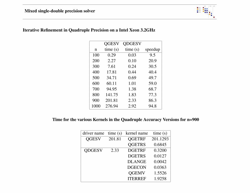
Iterative Refinement in Quadruple Precision on a Intel Xeon 3.2GHz
QGESV QDGESVn time (s) time (s) speedup
100 0.29 0.03 9.5200 2.27 0.10 20.9300 7.61 0.24 30.5400 17.81 0.44 40.4500 34.71 0.69 49.7600 60.11 1.01 59.0700 94.95 1.38 68.7800 141.75 1.83 77.3900 201.81 2.33 86.31000 276.94 2.92 94.8
Time for the various Kernels in the Quadruple Accuracy Versions for n=900
driver name time (s) kernel name time (s)QGESV 201.81 QGETRF 201.1293
QGETRS 0.6845QDGESV 2.33 DGETRF 0.3200
DGETRS 0.0127DLANGE 0.0042DGECON 0.0363QGEMV 1.5526ITERREF 1.9258

Mixed single-double precision solver
Extension to Other Algorithms
• As a rule of thumb, any algorithm with O(n3) computation and O(n) output can benefit from mixed precisioniterative refinement. (Idea: the residual computation needs to be at most O(n2).)
• This is not the case for eigendecomposition, SVD, matrix-matrix multiplication. This is the case for linearsystem of equations solve.
• – J. J. Dongarra, C. B. Moler and J. H. Wilkinson, Improving the Accuracy of Computed Eigenvalues andEigenvectors, SIAM Journal on Numerical Analysis, 20(1):23-45, 1983.
– J. J. Dongarra, Improving the Accuracy of Computed Singular Values, SIAM Journal on Scientific andStatistical Computing, 4(4):712-719, 1983.
– J. J.Dongarra, Algorithm 589: SICEDR: A FORTRAN Subroutine for Improving the Accuracy of Com-puted Matrix Eigenvalues, ACM Transactions on Mathematical Software, 8(4):371-375, 1982.

Mixed single-double precision solver
Julien Langou, University of Colorado Denver.
Mixed single-double precision solverWednesday April 1st, 2008.
1. Mixed single-double precision solver2. Rectangular Full Packed Format3. Communication optimal algorithm

Mixed single-double precision solver
F. G. Gustavson, J. Wasniewski, J. J. Dongarra, and Julien Langou.Rectangular Full Packed Format for Cholesky’s Algorithm: Factorization, Solution and Inversion.arXiv:0901.1696.

Mixed single-double precision solver
Case n is odd (n= 7), TRANSR = ’N’, UPLO = ’L’
COMPLEX Rectangular Full Packed Format.
EIGHT cases: N is ODD or EVEN TRANSR = 'L' or TRANSR = 'C' UPLO = 'L' or UPLO = 'U'
COMPLEX => entries are complex numbers. They are represented below by ( REAL_PART, IMAG_PART ).
On the LEFT: example matrix in Full Format (so ZHE, ZSY, ZTR), the entry (***,***) represents unreference memory spaces.On the RIGHT: example matrix in Rectangular Full Packed Format (so ZHF, ZSF, ZTF)
The GREEN entries represents the part of the matrix that is not tranpose in the RFP format.The RED entries represents the part of the matrix that is conjugate-tranpose in the RFP format.
This web page is automatically generated by the following C-code: visualize_html.tar.gz.( There is also a TERMINAL version with colors :) visualize_terminal.tar.gz. )
Case n is odd (n= 7), TRANSR = 'N', UPLO = 'L'
( +0,+97) (***,***) (***,***) (***,***) (***,***) (***,***) (***,***) ( +0,+97) (+32,-65) (+33,-64) (+34,-63) ( +1,+96) ( +8,+89) (***,***) (***,***) (***,***) (***,***) (***,***) ( +1,+96) ( +8,+89) (+40,-57) (+41,-56) ( +2,+95) ( +9,+88) (+16,+81) (***,***) (***,***) (***,***) (***,***) ( +2,+95) ( +9,+88) (+16,+81) (+48,-49) ( +3,+94) (+10,+87) (+17,+80) (+24,+73) (***,***) (***,***) (***,***) ====== > ( +3,+94) (+10,+87) (+17,+80) (+24,+73) ( +4,+93) (+11,+86) (+18,+79) (+25,+72) (+32,+65) (***,***) (***,***) ( +4,+93) (+11,+86) (+18,+79) (+25,+72) ( +5,+92) (+12,+85) (+19,+78) (+26,+71) (+33,+64) (+40,+57) (***,***) ( +5,+92) (+12,+85) (+19,+78) (+26,+71) ( +6,+91) (+13,+84) (+20,+77) (+27,+70) (+34,+63) (+41,+56) (+48,+49) ( +6,+91) (+13,+84) (+20,+77) (+27,+70)
Case n is odd (n= 7), TRANSR = 'N', UPLO = 'U'
( +0,+97) ( +7,+90) (+14,+83) (+21,+76) (+28,+69) (+35,+62) (+42,+55) (+21,+76) (+28,+69) (+35,+62) (+42,+55) (***,***) ( +8,+89) (+15,+82) (+22,+75) (+29,+68) (+36,+61) (+43,+54) (+22,+75) (+29,+68) (+36,+61) (+43,+54) (***,***) (***,***) (+16,+81) (+23,+74) (+30,+67) (+37,+60) (+44,+53) (+23,+74) (+30,+67) (+37,+60) (+44,+53) (***,***) (***,***) (***,***) (+24,+73) (+31,+66) (+38,+59) (+45,+52) ====== > (+24,+73) (+31,+66) (+38,+59) (+45,+52) (***,***) (***,***) (***,***) (***,***) (+32,+65) (+39,+58) (+46,+51) ( +0,-97) (+32,+65) (+39,+58) (+46,+51) (***,***) (***,***) (***,***) (***,***) (***,***) (+40,+57) (+47,+50) ( +7,-90) ( +8,-89) (+40,+57) (+47,+50) (***,***) (***,***) (***,***) (***,***) (***,***) (***,***) (+48,+49) (+14,-83) (+15,-82) (+16,-81) (+48,+49)
Case n is odd (n= 7), TRANSR = 'C', UPLO = 'L'
( +0,+97) (***,***) (***,***) (***,***) (***,***) (***,***) (***,***) ( +0,-97) ( +1,-96) ( +2,-95) ( +3,-94) ( +4,-93) ( +5,-92) ( +6,-91) ( +1,+96) ( +8,+89) (***,***) (***,***) (***,***) (***,***) (***,***) (+32,+65) ( +8,-89) ( +9,-88) (+10,-87) (+11,-86) (+12,-85) (+13,-84) ( +2,+95) ( +9,+88) (+16,+81) (***,***) (***,***) (***,***) (***,***) (+33,+64) (+40,+57) (+16,-81) (+17,-80) (+18,-79) (+19,-78) (+20,-77) ( +3,+94) (+10,+87) (+17,+80) (+24,+73) (***,***) (***,***) (***,***) ====== > (+34,+63) (+41,+56) (+48,+49) (+24,-73) (+25,-72) (+26,-71) (+27,-70) ( +4,+93) (+11,+86) (+18,+79) (+25,+72) (+32,+65) (***,***) (***,***) ( +5,+92) (+12,+85) (+19,+78) (+26,+71) (+33,+64) (+40,+57) (***,***) ( +6,+91) (+13,+84) (+20,+77) (+27,+70) (+34,+63) (+41,+56) (+48,+49)
Case n is odd (n= 7), TRANSR = 'C', UPLO = 'U'
( +0,+97) ( +7,+90) (+14,+83) (+21,+76) (+28,+69) (+35,+62) (+42,+55) (+21,-76) (+22,-75) (+23,-74) (+24,-73) ( +0,+97) ( +7,+90) (+14,+83) (***,***) ( +8,+89) (+15,+82) (+22,+75) (+29,+68) (+36,+61) (+43,+54) (+28,-69) (+29,-68) (+30,-67) (+31,-66) (+32,-65) ( +8,+89) (+15,+82) (***,***) (***,***) (+16,+81) (+23,+74) (+30,+67) (+37,+60) (+44,+53) (+35,-62) (+36,-61) (+37,-60) (+38,-59) (+39,-58) (+40,-57) (+16,+81) (***,***) (***,***) (***,***) (+24,+73) (+31,+66) (+38,+59) (+45,+52) ====== > (+42,-55) (+43,-54) (+44,-53) (+45,-52) (+46,-51) (+47,-50) (+48,-49) (***,***) (***,***) (***,***) (***,***) (+32,+65) (+39,+58) (+46,+51) (***,***) (***,***) (***,***) (***,***) (***,***) (+40,+57) (+47,+50) (***,***) (***,***) (***,***) (***,***) (***,***) (***,***) (+48,+49)
Case n is even (n= 6), TRANSR = 'N', UPLO = 'L'
( +0,+71) (***,***) (***,***) (***,***) (***,***) (***,***) (+21,-50) (+22,-49) (+23,-48)
Case n is odd (n= 7), TRANSR = ’N’, UPLO = ’U’
COMPLEX Rectangular Full Packed Format.
EIGHT cases: N is ODD or EVEN TRANSR = 'L' or TRANSR = 'C' UPLO = 'L' or UPLO = 'U'
COMPLEX => entries are complex numbers. They are represented below by ( REAL_PART, IMAG_PART ).
On the LEFT: example matrix in Full Format (so ZHE, ZSY, ZTR), the entry (***,***) represents unreference memory spaces.On the RIGHT: example matrix in Rectangular Full Packed Format (so ZHF, ZSF, ZTF)
The GREEN entries represents the part of the matrix that is not tranpose in the RFP format.The RED entries represents the part of the matrix that is conjugate-tranpose in the RFP format.
This web page is automatically generated by the following C-code: visualize_html.tar.gz.( There is also a TERMINAL version with colors :) visualize_terminal.tar.gz. )
Case n is odd (n= 7), TRANSR = 'N', UPLO = 'L'
( +0,+97) (***,***) (***,***) (***,***) (***,***) (***,***) (***,***) ( +0,+97) (+32,-65) (+33,-64) (+34,-63) ( +1,+96) ( +8,+89) (***,***) (***,***) (***,***) (***,***) (***,***) ( +1,+96) ( +8,+89) (+40,-57) (+41,-56) ( +2,+95) ( +9,+88) (+16,+81) (***,***) (***,***) (***,***) (***,***) ( +2,+95) ( +9,+88) (+16,+81) (+48,-49) ( +3,+94) (+10,+87) (+17,+80) (+24,+73) (***,***) (***,***) (***,***) ====== > ( +3,+94) (+10,+87) (+17,+80) (+24,+73) ( +4,+93) (+11,+86) (+18,+79) (+25,+72) (+32,+65) (***,***) (***,***) ( +4,+93) (+11,+86) (+18,+79) (+25,+72) ( +5,+92) (+12,+85) (+19,+78) (+26,+71) (+33,+64) (+40,+57) (***,***) ( +5,+92) (+12,+85) (+19,+78) (+26,+71) ( +6,+91) (+13,+84) (+20,+77) (+27,+70) (+34,+63) (+41,+56) (+48,+49) ( +6,+91) (+13,+84) (+20,+77) (+27,+70)
Case n is odd (n= 7), TRANSR = 'N', UPLO = 'U'
( +0,+97) ( +7,+90) (+14,+83) (+21,+76) (+28,+69) (+35,+62) (+42,+55) (+21,+76) (+28,+69) (+35,+62) (+42,+55) (***,***) ( +8,+89) (+15,+82) (+22,+75) (+29,+68) (+36,+61) (+43,+54) (+22,+75) (+29,+68) (+36,+61) (+43,+54) (***,***) (***,***) (+16,+81) (+23,+74) (+30,+67) (+37,+60) (+44,+53) (+23,+74) (+30,+67) (+37,+60) (+44,+53) (***,***) (***,***) (***,***) (+24,+73) (+31,+66) (+38,+59) (+45,+52) ====== > (+24,+73) (+31,+66) (+38,+59) (+45,+52) (***,***) (***,***) (***,***) (***,***) (+32,+65) (+39,+58) (+46,+51) ( +0,-97) (+32,+65) (+39,+58) (+46,+51) (***,***) (***,***) (***,***) (***,***) (***,***) (+40,+57) (+47,+50) ( +7,-90) ( +8,-89) (+40,+57) (+47,+50) (***,***) (***,***) (***,***) (***,***) (***,***) (***,***) (+48,+49) (+14,-83) (+15,-82) (+16,-81) (+48,+49)
Case n is odd (n= 7), TRANSR = 'C', UPLO = 'L'
( +0,+97) (***,***) (***,***) (***,***) (***,***) (***,***) (***,***) ( +0,-97) ( +1,-96) ( +2,-95) ( +3,-94) ( +4,-93) ( +5,-92) ( +6,-91) ( +1,+96) ( +8,+89) (***,***) (***,***) (***,***) (***,***) (***,***) (+32,+65) ( +8,-89) ( +9,-88) (+10,-87) (+11,-86) (+12,-85) (+13,-84) ( +2,+95) ( +9,+88) (+16,+81) (***,***) (***,***) (***,***) (***,***) (+33,+64) (+40,+57) (+16,-81) (+17,-80) (+18,-79) (+19,-78) (+20,-77) ( +3,+94) (+10,+87) (+17,+80) (+24,+73) (***,***) (***,***) (***,***) ====== > (+34,+63) (+41,+56) (+48,+49) (+24,-73) (+25,-72) (+26,-71) (+27,-70) ( +4,+93) (+11,+86) (+18,+79) (+25,+72) (+32,+65) (***,***) (***,***) ( +5,+92) (+12,+85) (+19,+78) (+26,+71) (+33,+64) (+40,+57) (***,***) ( +6,+91) (+13,+84) (+20,+77) (+27,+70) (+34,+63) (+41,+56) (+48,+49)
Case n is odd (n= 7), TRANSR = 'C', UPLO = 'U'
( +0,+97) ( +7,+90) (+14,+83) (+21,+76) (+28,+69) (+35,+62) (+42,+55) (+21,-76) (+22,-75) (+23,-74) (+24,-73) ( +0,+97) ( +7,+90) (+14,+83) (***,***) ( +8,+89) (+15,+82) (+22,+75) (+29,+68) (+36,+61) (+43,+54) (+28,-69) (+29,-68) (+30,-67) (+31,-66) (+32,-65) ( +8,+89) (+15,+82) (***,***) (***,***) (+16,+81) (+23,+74) (+30,+67) (+37,+60) (+44,+53) (+35,-62) (+36,-61) (+37,-60) (+38,-59) (+39,-58) (+40,-57) (+16,+81) (***,***) (***,***) (***,***) (+24,+73) (+31,+66) (+38,+59) (+45,+52) ====== > (+42,-55) (+43,-54) (+44,-53) (+45,-52) (+46,-51) (+47,-50) (+48,-49) (***,***) (***,***) (***,***) (***,***) (+32,+65) (+39,+58) (+46,+51) (***,***) (***,***) (***,***) (***,***) (***,***) (+40,+57) (+47,+50) (***,***) (***,***) (***,***) (***,***) (***,***) (***,***) (+48,+49)
Case n is even (n= 6), TRANSR = 'N', UPLO = 'L'
( +0,+71) (***,***) (***,***) (***,***) (***,***) (***,***) (+21,-50) (+22,-49) (+23,-48)
Case n is odd (n= 7), TRANSR = ’C’, UPLO = ’L’
COMPLEX Rectangular Full Packed Format.
EIGHT cases: N is ODD or EVEN TRANSR = 'L' or TRANSR = 'C' UPLO = 'L' or UPLO = 'U'
COMPLEX => entries are complex numbers. They are represented below by ( REAL_PART, IMAG_PART ).
On the LEFT: example matrix in Full Format (so ZHE, ZSY, ZTR), the entry (***,***) represents unreference memory spaces.On the RIGHT: example matrix in Rectangular Full Packed Format (so ZHF, ZSF, ZTF)
The GREEN entries represents the part of the matrix that is not tranpose in the RFP format.The RED entries represents the part of the matrix that is conjugate-tranpose in the RFP format.
This web page is automatically generated by the following C-code: visualize_html.tar.gz.( There is also a TERMINAL version with colors :) visualize_terminal.tar.gz. )
Case n is odd (n= 7), TRANSR = 'N', UPLO = 'L'
( +0,+97) (***,***) (***,***) (***,***) (***,***) (***,***) (***,***) ( +0,+97) (+32,-65) (+33,-64) (+34,-63) ( +1,+96) ( +8,+89) (***,***) (***,***) (***,***) (***,***) (***,***) ( +1,+96) ( +8,+89) (+40,-57) (+41,-56) ( +2,+95) ( +9,+88) (+16,+81) (***,***) (***,***) (***,***) (***,***) ( +2,+95) ( +9,+88) (+16,+81) (+48,-49) ( +3,+94) (+10,+87) (+17,+80) (+24,+73) (***,***) (***,***) (***,***) ====== > ( +3,+94) (+10,+87) (+17,+80) (+24,+73) ( +4,+93) (+11,+86) (+18,+79) (+25,+72) (+32,+65) (***,***) (***,***) ( +4,+93) (+11,+86) (+18,+79) (+25,+72) ( +5,+92) (+12,+85) (+19,+78) (+26,+71) (+33,+64) (+40,+57) (***,***) ( +5,+92) (+12,+85) (+19,+78) (+26,+71) ( +6,+91) (+13,+84) (+20,+77) (+27,+70) (+34,+63) (+41,+56) (+48,+49) ( +6,+91) (+13,+84) (+20,+77) (+27,+70)
Case n is odd (n= 7), TRANSR = 'N', UPLO = 'U'
( +0,+97) ( +7,+90) (+14,+83) (+21,+76) (+28,+69) (+35,+62) (+42,+55) (+21,+76) (+28,+69) (+35,+62) (+42,+55) (***,***) ( +8,+89) (+15,+82) (+22,+75) (+29,+68) (+36,+61) (+43,+54) (+22,+75) (+29,+68) (+36,+61) (+43,+54) (***,***) (***,***) (+16,+81) (+23,+74) (+30,+67) (+37,+60) (+44,+53) (+23,+74) (+30,+67) (+37,+60) (+44,+53) (***,***) (***,***) (***,***) (+24,+73) (+31,+66) (+38,+59) (+45,+52) ====== > (+24,+73) (+31,+66) (+38,+59) (+45,+52) (***,***) (***,***) (***,***) (***,***) (+32,+65) (+39,+58) (+46,+51) ( +0,-97) (+32,+65) (+39,+58) (+46,+51) (***,***) (***,***) (***,***) (***,***) (***,***) (+40,+57) (+47,+50) ( +7,-90) ( +8,-89) (+40,+57) (+47,+50) (***,***) (***,***) (***,***) (***,***) (***,***) (***,***) (+48,+49) (+14,-83) (+15,-82) (+16,-81) (+48,+49)
Case n is odd (n= 7), TRANSR = 'C', UPLO = 'L'
( +0,+97) (***,***) (***,***) (***,***) (***,***) (***,***) (***,***) ( +0,-97) ( +1,-96) ( +2,-95) ( +3,-94) ( +4,-93) ( +5,-92) ( +6,-91) ( +1,+96) ( +8,+89) (***,***) (***,***) (***,***) (***,***) (***,***) (+32,+65) ( +8,-89) ( +9,-88) (+10,-87) (+11,-86) (+12,-85) (+13,-84) ( +2,+95) ( +9,+88) (+16,+81) (***,***) (***,***) (***,***) (***,***) (+33,+64) (+40,+57) (+16,-81) (+17,-80) (+18,-79) (+19,-78) (+20,-77) ( +3,+94) (+10,+87) (+17,+80) (+24,+73) (***,***) (***,***) (***,***) ====== > (+34,+63) (+41,+56) (+48,+49) (+24,-73) (+25,-72) (+26,-71) (+27,-70) ( +4,+93) (+11,+86) (+18,+79) (+25,+72) (+32,+65) (***,***) (***,***) ( +5,+92) (+12,+85) (+19,+78) (+26,+71) (+33,+64) (+40,+57) (***,***) ( +6,+91) (+13,+84) (+20,+77) (+27,+70) (+34,+63) (+41,+56) (+48,+49)
Case n is odd (n= 7), TRANSR = 'C', UPLO = 'U'
( +0,+97) ( +7,+90) (+14,+83) (+21,+76) (+28,+69) (+35,+62) (+42,+55) (+21,-76) (+22,-75) (+23,-74) (+24,-73) ( +0,+97) ( +7,+90) (+14,+83) (***,***) ( +8,+89) (+15,+82) (+22,+75) (+29,+68) (+36,+61) (+43,+54) (+28,-69) (+29,-68) (+30,-67) (+31,-66) (+32,-65) ( +8,+89) (+15,+82) (***,***) (***,***) (+16,+81) (+23,+74) (+30,+67) (+37,+60) (+44,+53) (+35,-62) (+36,-61) (+37,-60) (+38,-59) (+39,-58) (+40,-57) (+16,+81) (***,***) (***,***) (***,***) (+24,+73) (+31,+66) (+38,+59) (+45,+52) ====== > (+42,-55) (+43,-54) (+44,-53) (+45,-52) (+46,-51) (+47,-50) (+48,-49) (***,***) (***,***) (***,***) (***,***) (+32,+65) (+39,+58) (+46,+51) (***,***) (***,***) (***,***) (***,***) (***,***) (+40,+57) (+47,+50) (***,***) (***,***) (***,***) (***,***) (***,***) (***,***) (+48,+49)
Case n is even (n= 6), TRANSR = 'N', UPLO = 'L'
( +0,+71) (***,***) (***,***) (***,***) (***,***) (***,***) (+21,-50) (+22,-49) (+23,-48)
Case n is odd (n= 7), TRANSR = ’C’, UPLO = ’U’
COMPLEX Rectangular Full Packed Format.
EIGHT cases: N is ODD or EVEN TRANSR = 'L' or TRANSR = 'C' UPLO = 'L' or UPLO = 'U'
COMPLEX => entries are complex numbers. They are represented below by ( REAL_PART, IMAG_PART ).
On the LEFT: example matrix in Full Format (so ZHE, ZSY, ZTR), the entry (***,***) represents unreference memory spaces.On the RIGHT: example matrix in Rectangular Full Packed Format (so ZHF, ZSF, ZTF)
The GREEN entries represents the part of the matrix that is not tranpose in the RFP format.The RED entries represents the part of the matrix that is conjugate-tranpose in the RFP format.
This web page is automatically generated by the following C-code: visualize_html.tar.gz.( There is also a TERMINAL version with colors :) visualize_terminal.tar.gz. )
Case n is odd (n= 7), TRANSR = 'N', UPLO = 'L'
( +0,+97) (***,***) (***,***) (***,***) (***,***) (***,***) (***,***) ( +0,+97) (+32,-65) (+33,-64) (+34,-63) ( +1,+96) ( +8,+89) (***,***) (***,***) (***,***) (***,***) (***,***) ( +1,+96) ( +8,+89) (+40,-57) (+41,-56) ( +2,+95) ( +9,+88) (+16,+81) (***,***) (***,***) (***,***) (***,***) ( +2,+95) ( +9,+88) (+16,+81) (+48,-49) ( +3,+94) (+10,+87) (+17,+80) (+24,+73) (***,***) (***,***) (***,***) ====== > ( +3,+94) (+10,+87) (+17,+80) (+24,+73) ( +4,+93) (+11,+86) (+18,+79) (+25,+72) (+32,+65) (***,***) (***,***) ( +4,+93) (+11,+86) (+18,+79) (+25,+72) ( +5,+92) (+12,+85) (+19,+78) (+26,+71) (+33,+64) (+40,+57) (***,***) ( +5,+92) (+12,+85) (+19,+78) (+26,+71) ( +6,+91) (+13,+84) (+20,+77) (+27,+70) (+34,+63) (+41,+56) (+48,+49) ( +6,+91) (+13,+84) (+20,+77) (+27,+70)
Case n is odd (n= 7), TRANSR = 'N', UPLO = 'U'
( +0,+97) ( +7,+90) (+14,+83) (+21,+76) (+28,+69) (+35,+62) (+42,+55) (+21,+76) (+28,+69) (+35,+62) (+42,+55) (***,***) ( +8,+89) (+15,+82) (+22,+75) (+29,+68) (+36,+61) (+43,+54) (+22,+75) (+29,+68) (+36,+61) (+43,+54) (***,***) (***,***) (+16,+81) (+23,+74) (+30,+67) (+37,+60) (+44,+53) (+23,+74) (+30,+67) (+37,+60) (+44,+53) (***,***) (***,***) (***,***) (+24,+73) (+31,+66) (+38,+59) (+45,+52) ====== > (+24,+73) (+31,+66) (+38,+59) (+45,+52) (***,***) (***,***) (***,***) (***,***) (+32,+65) (+39,+58) (+46,+51) ( +0,-97) (+32,+65) (+39,+58) (+46,+51) (***,***) (***,***) (***,***) (***,***) (***,***) (+40,+57) (+47,+50) ( +7,-90) ( +8,-89) (+40,+57) (+47,+50) (***,***) (***,***) (***,***) (***,***) (***,***) (***,***) (+48,+49) (+14,-83) (+15,-82) (+16,-81) (+48,+49)
Case n is odd (n= 7), TRANSR = 'C', UPLO = 'L'
( +0,+97) (***,***) (***,***) (***,***) (***,***) (***,***) (***,***) ( +0,-97) ( +1,-96) ( +2,-95) ( +3,-94) ( +4,-93) ( +5,-92) ( +6,-91) ( +1,+96) ( +8,+89) (***,***) (***,***) (***,***) (***,***) (***,***) (+32,+65) ( +8,-89) ( +9,-88) (+10,-87) (+11,-86) (+12,-85) (+13,-84) ( +2,+95) ( +9,+88) (+16,+81) (***,***) (***,***) (***,***) (***,***) (+33,+64) (+40,+57) (+16,-81) (+17,-80) (+18,-79) (+19,-78) (+20,-77) ( +3,+94) (+10,+87) (+17,+80) (+24,+73) (***,***) (***,***) (***,***) ====== > (+34,+63) (+41,+56) (+48,+49) (+24,-73) (+25,-72) (+26,-71) (+27,-70) ( +4,+93) (+11,+86) (+18,+79) (+25,+72) (+32,+65) (***,***) (***,***) ( +5,+92) (+12,+85) (+19,+78) (+26,+71) (+33,+64) (+40,+57) (***,***) ( +6,+91) (+13,+84) (+20,+77) (+27,+70) (+34,+63) (+41,+56) (+48,+49)
Case n is odd (n= 7), TRANSR = 'C', UPLO = 'U'
( +0,+97) ( +7,+90) (+14,+83) (+21,+76) (+28,+69) (+35,+62) (+42,+55) (+21,-76) (+22,-75) (+23,-74) (+24,-73) ( +0,+97) ( +7,+90) (+14,+83) (***,***) ( +8,+89) (+15,+82) (+22,+75) (+29,+68) (+36,+61) (+43,+54) (+28,-69) (+29,-68) (+30,-67) (+31,-66) (+32,-65) ( +8,+89) (+15,+82) (***,***) (***,***) (+16,+81) (+23,+74) (+30,+67) (+37,+60) (+44,+53) (+35,-62) (+36,-61) (+37,-60) (+38,-59) (+39,-58) (+40,-57) (+16,+81) (***,***) (***,***) (***,***) (+24,+73) (+31,+66) (+38,+59) (+45,+52) ====== > (+42,-55) (+43,-54) (+44,-53) (+45,-52) (+46,-51) (+47,-50) (+48,-49) (***,***) (***,***) (***,***) (***,***) (+32,+65) (+39,+58) (+46,+51) (***,***) (***,***) (***,***) (***,***) (***,***) (+40,+57) (+47,+50) (***,***) (***,***) (***,***) (***,***) (***,***) (***,***) (+48,+49)
Case n is even (n= 6), TRANSR = 'N', UPLO = 'L'
( +0,+71) (***,***) (***,***) (***,***) (***,***) (***,***) (+21,-50) (+22,-49) (+23,-48)

Mixed single-double precision solver
Case n is even (n= 6), TRANSR = ’N’, UPLO = ’L’
COMPLEX Rectangular Full Packed Format.
EIGHT cases: N is ODD or EVEN TRANSR = 'L' or TRANSR = 'C' UPLO = 'L' or UPLO = 'U'
COMPLEX => entries are complex numbers. They are represented below by ( REAL_PART, IMAG_PART ).
On the LEFT: example matrix in Full Format (so ZHE, ZSY, ZTR), the entry (***,***) represents unreference memory spaces.On the RIGHT: example matrix in Rectangular Full Packed Format (so ZHF, ZSF, ZTF)
The GREEN entries represents the part of the matrix that is not tranpose in the RFP format.The RED entries represents the part of the matrix that is conjugate-tranpose in the RFP format.
This web page is automatically generated by the following C-code: visualize_html.tar.gz.( There is also a TERMINAL version with colors :) visualize_terminal.tar.gz. )
Case n is odd (n= 7), TRANSR = 'N', UPLO = 'U'
( +0,+97) ( +7,+90) (+14,+83) (+21,+76) (+28,+69) (+35,+62) (+42,+55) (+21,+76) (+28,+69) (+35,+62) (+42,+55) (***,***) ( +8,+89) (+15,+82) (+22,+75) (+29,+68) (+36,+61) (+43,+54) (+22,+75) (+29,+68) (+36,+61) (+43,+54) (***,***) (***,***) (+16,+81) (+23,+74) (+30,+67) (+37,+60) (+44,+53) (+23,+74) (+30,+67) (+37,+60) (+44,+53) (***,***) (***,***) (***,***) (+24,+73) (+31,+66) (+38,+59) (+45,+52) ====== > (+24,+73) (+31,+66) (+38,+59) (+45,+52) (***,***) (***,***) (***,***) (***,***) (+32,+65) (+39,+58) (+46,+51) ( +0,-97) (+32,+65) (+39,+58) (+46,+51) (***,***) (***,***) (***,***) (***,***) (***,***) (+40,+57) (+47,+50) ( +7,-90) ( +8,-89) (+40,+57) (+47,+50) (***,***) (***,***) (***,***) (***,***) (***,***) (***,***) (+48,+49) (+14,-83) (+15,-82) (+16,-81) (+48,+49)
Case n is odd (n= 7), TRANSR = 'C', UPLO = 'L'
( +0,+97) (***,***) (***,***) (***,***) (***,***) (***,***) (***,***) ( +0,-97) ( +1,-96) ( +2,-95) ( +3,-94) ( +4,-93) ( +5,-92) ( +6,-91) ( +1,+96) ( +8,+89) (***,***) (***,***) (***,***) (***,***) (***,***) (+32,+65) ( +8,-89) ( +9,-88) (+10,-87) (+11,-86) (+12,-85) (+13,-84) ( +2,+95) ( +9,+88) (+16,+81) (***,***) (***,***) (***,***) (***,***) (+33,+64) (+40,+57) (+16,-81) (+17,-80) (+18,-79) (+19,-78) (+20,-77) ( +3,+94) (+10,+87) (+17,+80) (+24,+73) (***,***) (***,***) (***,***) ====== > (+34,+63) (+41,+56) (+48,+49) (+24,-73) (+25,-72) (+26,-71) (+27,-70) ( +4,+93) (+11,+86) (+18,+79) (+25,+72) (+32,+65) (***,***) (***,***) ( +5,+92) (+12,+85) (+19,+78) (+26,+71) (+33,+64) (+40,+57) (***,***) ( +6,+91) (+13,+84) (+20,+77) (+27,+70) (+34,+63) (+41,+56) (+48,+49)
Case n is odd (n= 7), TRANSR = 'C', UPLO = 'U'
( +0,+97) ( +7,+90) (+14,+83) (+21,+76) (+28,+69) (+35,+62) (+42,+55) (+21,-76) (+22,-75) (+23,-74) (+24,-73) ( +0,+97) ( +7,+90) (+14,+83) (***,***) ( +8,+89) (+15,+82) (+22,+75) (+29,+68) (+36,+61) (+43,+54) (+28,-69) (+29,-68) (+30,-67) (+31,-66) (+32,-65) ( +8,+89) (+15,+82) (***,***) (***,***) (+16,+81) (+23,+74) (+30,+67) (+37,+60) (+44,+53) (+35,-62) (+36,-61) (+37,-60) (+38,-59) (+39,-58) (+40,-57) (+16,+81) (***,***) (***,***) (***,***) (+24,+73) (+31,+66) (+38,+59) (+45,+52) ====== > (+42,-55) (+43,-54) (+44,-53) (+45,-52) (+46,-51) (+47,-50) (+48,-49) (***,***) (***,***) (***,***) (***,***) (+32,+65) (+39,+58) (+46,+51) (***,***) (***,***) (***,***) (***,***) (***,***) (+40,+57) (+47,+50) (***,***) (***,***) (***,***) (***,***) (***,***) (***,***) (+48,+49)
Case n is even (n= 6), TRANSR = 'N', UPLO = 'L'
( +0,+71) (***,***) (***,***) (***,***) (***,***) (***,***) (+21,-50) (+22,-49) (+23,-48) ( +1,+70) ( +7,+64) (***,***) (***,***) (***,***) (***,***) ( +0,+71) (+28,-43) (+29,-42) ( +2,+69) ( +8,+63) (+14,+57) (***,***) (***,***) (***,***) ( +1,+70) ( +7,+64) (+35,-36) ( +3,+68) ( +9,+62) (+15,+56) (+21,+50) (***,***) (***,***) ====== > ( +2,+69) ( +8,+63) (+14,+57) ( +4,+67) (+10,+61) (+16,+55) (+22,+49) (+28,+43) (***,***) ( +3,+68) ( +9,+62) (+15,+56) ( +5,+66) (+11,+60) (+17,+54) (+23,+48) (+29,+42) (+35,+36) ( +4,+67) (+10,+61) (+16,+55) ( +5,+66) (+11,+60) (+17,+54)
Case n is even (n= 6), TRANSR = 'N', UPLO = 'U'
( +0,+71) ( +6,+65) (+12,+59) (+18,+53) (+24,+47) (+30,+41) (+18,+53) (+24,+47) (+30,+41) (***,***) ( +7,+64) (+13,+58) (+19,+52) (+25,+46) (+31,+40) (+19,+52) (+25,+46) (+31,+40)
Case n is even (n= 6), TRANSR = ’N’, UPLO = ’U’
( +1,+70) ( +7,+64) (***,***) (***,***) (***,***) (***,***) ( +0,+71) (+28,-43) (+29,-42) ( +2,+69) ( +8,+63) (+14,+57) (***,***) (***,***) (***,***) ( +1,+70) ( +7,+64) (+35,-36) ( +3,+68) ( +9,+62) (+15,+56) (+21,+50) (***,***) (***,***) ====== > ( +2,+69) ( +8,+63) (+14,+57) ( +4,+67) (+10,+61) (+16,+55) (+22,+49) (+28,+43) (***,***) ( +3,+68) ( +9,+62) (+15,+56) ( +5,+66) (+11,+60) (+17,+54) (+23,+48) (+29,+42) (+35,+36) ( +4,+67) (+10,+61) (+16,+55) ( +5,+66) (+11,+60) (+17,+54)
Case n is even (n= 6), TRANSR = 'N', UPLO = 'U'
( +0,+71) ( +6,+65) (+12,+59) (+18,+53) (+24,+47) (+30,+41) (+18,+53) (+24,+47) (+30,+41) (***,***) ( +7,+64) (+13,+58) (+19,+52) (+25,+46) (+31,+40) (+19,+52) (+25,+46) (+31,+40) (***,***) (***,***) (+14,+57) (+20,+51) (+26,+45) (+32,+39) (+20,+51) (+26,+45) (+32,+39) (***,***) (***,***) (***,***) (+21,+50) (+27,+44) (+33,+38) ====== > (+21,+50) (+27,+44) (+33,+38) (***,***) (***,***) (***,***) (***,***) (+28,+43) (+34,+37) ( +0,-71) (+28,+43) (+34,+37) (***,***) (***,***) (***,***) (***,***) (***,***) (+35,+36) ( +6,-65) ( +7,-64) (+35,+36) (+12,-59) (+13,-58) (+14,-57)
Case n is even (n= 6), TRANSR = 'C', UPLO = 'L'
( +0,+71) (***,***) (***,***) (***,***) (***,***) (***,***) (+21,+50) ( +0,-71) ( +1,-70) ( +2,-69) ( +3,-68) ( +4,-67) ( +5,-66) ( +1,+70) ( +7,+64) (***,***) (***,***) (***,***) (***,***) (+22,+49) (+28,+43) ( +7,-64) ( +8,-63) ( +9,-62) (+10,-61) (+11,-60) ( +2,+69) ( +8,+63) (+14,+57) (***,***) (***,***) (***,***) (+23,+48) (+29,+42) (+35,+36) (+14,-57) (+15,-56) (+16,-55) (+17,-54) ( +3,+68) ( +9,+62) (+15,+56) (+21,+50) (***,***) (***,***) ====== > ( +4,+67) (+10,+61) (+16,+55) (+22,+49) (+28,+43) (***,***) ( +5,+66) (+11,+60) (+17,+54) (+23,+48) (+29,+42) (+35,+36)
Case n is even (n= 6), TRANSR = 'C', UPLO = 'U'
( +0,+71) ( +6,+65) (+12,+59) (+18,+53) (+24,+47) (+30,+41) (+18,-53) (+19,-52) (+20,-51) (+21,-50) ( +0,+71) ( +6,+65) (+12,+59) (***,***) ( +7,+64) (+13,+58) (+19,+52) (+25,+46) (+31,+40) (+24,-47) (+25,-46) (+26,-45) (+27,-44) (+28,-43) ( +7,+64) (+13,+58) (***,***) (***,***) (+14,+57) (+20,+51) (+26,+45) (+32,+39) (+30,-41) (+31,-40) (+32,-39) (+33,-38) (+34,-37) (+35,-36) (+14,+57) (***,***) (***,***) (***,***) (+21,+50) (+27,+44) (+33,+38) ====== > (***,***) (***,***) (***,***) (***,***) (+28,+43) (+34,+37) (***,***) (***,***) (***,***) (***,***) (***,***) (+35,+36)
Case n is even (n= 6), TRANSR = ’C’, UPLO = ’L’
( +1,+70) ( +7,+64) (***,***) (***,***) (***,***) (***,***) ( +0,+71) (+28,-43) (+29,-42) ( +2,+69) ( +8,+63) (+14,+57) (***,***) (***,***) (***,***) ( +1,+70) ( +7,+64) (+35,-36) ( +3,+68) ( +9,+62) (+15,+56) (+21,+50) (***,***) (***,***) ====== > ( +2,+69) ( +8,+63) (+14,+57) ( +4,+67) (+10,+61) (+16,+55) (+22,+49) (+28,+43) (***,***) ( +3,+68) ( +9,+62) (+15,+56) ( +5,+66) (+11,+60) (+17,+54) (+23,+48) (+29,+42) (+35,+36) ( +4,+67) (+10,+61) (+16,+55) ( +5,+66) (+11,+60) (+17,+54)
Case n is even (n= 6), TRANSR = 'N', UPLO = 'U'
( +0,+71) ( +6,+65) (+12,+59) (+18,+53) (+24,+47) (+30,+41) (+18,+53) (+24,+47) (+30,+41) (***,***) ( +7,+64) (+13,+58) (+19,+52) (+25,+46) (+31,+40) (+19,+52) (+25,+46) (+31,+40) (***,***) (***,***) (+14,+57) (+20,+51) (+26,+45) (+32,+39) (+20,+51) (+26,+45) (+32,+39) (***,***) (***,***) (***,***) (+21,+50) (+27,+44) (+33,+38) ====== > (+21,+50) (+27,+44) (+33,+38) (***,***) (***,***) (***,***) (***,***) (+28,+43) (+34,+37) ( +0,-71) (+28,+43) (+34,+37) (***,***) (***,***) (***,***) (***,***) (***,***) (+35,+36) ( +6,-65) ( +7,-64) (+35,+36) (+12,-59) (+13,-58) (+14,-57)
Case n is even (n= 6), TRANSR = 'C', UPLO = 'L'
( +0,+71) (***,***) (***,***) (***,***) (***,***) (***,***) (+21,+50) ( +0,-71) ( +1,-70) ( +2,-69) ( +3,-68) ( +4,-67) ( +5,-66) ( +1,+70) ( +7,+64) (***,***) (***,***) (***,***) (***,***) (+22,+49) (+28,+43) ( +7,-64) ( +8,-63) ( +9,-62) (+10,-61) (+11,-60) ( +2,+69) ( +8,+63) (+14,+57) (***,***) (***,***) (***,***) (+23,+48) (+29,+42) (+35,+36) (+14,-57) (+15,-56) (+16,-55) (+17,-54) ( +3,+68) ( +9,+62) (+15,+56) (+21,+50) (***,***) (***,***) ====== > ( +4,+67) (+10,+61) (+16,+55) (+22,+49) (+28,+43) (***,***) ( +5,+66) (+11,+60) (+17,+54) (+23,+48) (+29,+42) (+35,+36)
Case n is even (n= 6), TRANSR = 'C', UPLO = 'U'
( +0,+71) ( +6,+65) (+12,+59) (+18,+53) (+24,+47) (+30,+41) (+18,-53) (+19,-52) (+20,-51) (+21,-50) ( +0,+71) ( +6,+65) (+12,+59) (***,***) ( +7,+64) (+13,+58) (+19,+52) (+25,+46) (+31,+40) (+24,-47) (+25,-46) (+26,-45) (+27,-44) (+28,-43) ( +7,+64) (+13,+58) (***,***) (***,***) (+14,+57) (+20,+51) (+26,+45) (+32,+39) (+30,-41) (+31,-40) (+32,-39) (+33,-38) (+34,-37) (+35,-36) (+14,+57) (***,***) (***,***) (***,***) (+21,+50) (+27,+44) (+33,+38) ====== > (***,***) (***,***) (***,***) (***,***) (+28,+43) (+34,+37) (***,***) (***,***) (***,***) (***,***) (***,***) (+35,+36)
Case n is even (n= 6), TRANSR = ’C’, UPLO = ’U’
( +1,+70) ( +7,+64) (***,***) (***,***) (***,***) (***,***) ( +0,+71) (+28,-43) (+29,-42) ( +2,+69) ( +8,+63) (+14,+57) (***,***) (***,***) (***,***) ( +1,+70) ( +7,+64) (+35,-36) ( +3,+68) ( +9,+62) (+15,+56) (+21,+50) (***,***) (***,***) ====== > ( +2,+69) ( +8,+63) (+14,+57) ( +4,+67) (+10,+61) (+16,+55) (+22,+49) (+28,+43) (***,***) ( +3,+68) ( +9,+62) (+15,+56) ( +5,+66) (+11,+60) (+17,+54) (+23,+48) (+29,+42) (+35,+36) ( +4,+67) (+10,+61) (+16,+55) ( +5,+66) (+11,+60) (+17,+54)
Case n is even (n= 6), TRANSR = 'N', UPLO = 'U'
( +0,+71) ( +6,+65) (+12,+59) (+18,+53) (+24,+47) (+30,+41) (+18,+53) (+24,+47) (+30,+41) (***,***) ( +7,+64) (+13,+58) (+19,+52) (+25,+46) (+31,+40) (+19,+52) (+25,+46) (+31,+40) (***,***) (***,***) (+14,+57) (+20,+51) (+26,+45) (+32,+39) (+20,+51) (+26,+45) (+32,+39) (***,***) (***,***) (***,***) (+21,+50) (+27,+44) (+33,+38) ====== > (+21,+50) (+27,+44) (+33,+38) (***,***) (***,***) (***,***) (***,***) (+28,+43) (+34,+37) ( +0,-71) (+28,+43) (+34,+37) (***,***) (***,***) (***,***) (***,***) (***,***) (+35,+36) ( +6,-65) ( +7,-64) (+35,+36) (+12,-59) (+13,-58) (+14,-57)
Case n is even (n= 6), TRANSR = 'C', UPLO = 'L'
( +0,+71) (***,***) (***,***) (***,***) (***,***) (***,***) (+21,+50) ( +0,-71) ( +1,-70) ( +2,-69) ( +3,-68) ( +4,-67) ( +5,-66) ( +1,+70) ( +7,+64) (***,***) (***,***) (***,***) (***,***) (+22,+49) (+28,+43) ( +7,-64) ( +8,-63) ( +9,-62) (+10,-61) (+11,-60) ( +2,+69) ( +8,+63) (+14,+57) (***,***) (***,***) (***,***) (+23,+48) (+29,+42) (+35,+36) (+14,-57) (+15,-56) (+16,-55) (+17,-54) ( +3,+68) ( +9,+62) (+15,+56) (+21,+50) (***,***) (***,***) ====== > ( +4,+67) (+10,+61) (+16,+55) (+22,+49) (+28,+43) (***,***) ( +5,+66) (+11,+60) (+17,+54) (+23,+48) (+29,+42) (+35,+36)
Case n is even (n= 6), TRANSR = 'C', UPLO = 'U'
( +0,+71) ( +6,+65) (+12,+59) (+18,+53) (+24,+47) (+30,+41) (+18,-53) (+19,-52) (+20,-51) (+21,-50) ( +0,+71) ( +6,+65) (+12,+59) (***,***) ( +7,+64) (+13,+58) (+19,+52) (+25,+46) (+31,+40) (+24,-47) (+25,-46) (+26,-45) (+27,-44) (+28,-43) ( +7,+64) (+13,+58) (***,***) (***,***) (+14,+57) (+20,+51) (+26,+45) (+32,+39) (+30,-41) (+31,-40) (+32,-39) (+33,-38) (+34,-37) (+35,-36) (+14,+57) (***,***) (***,***) (***,***) (+21,+50) (+27,+44) (+33,+38) ====== > (***,***) (***,***) (***,***) (***,***) (+28,+43) (+34,+37) (***,***) (***,***) (***,***) (***,***) (***,***) (+35,+36)

Mixed single-double precision solver
SUBROUTINE DPFTRF( TRANSR, UPLO, N, A, INFO )** -- LAPACK routine (version 3.2) --*
IF( NISODD ) THEN IF( NORMALTRANSR ) THEN IF( LOWER ) THEN* CALL DPOTRF( 'L', N1, A( 0 ), N, INFO ) IF( INFO.GT.0 ) + RETURN CALL DTRSM( 'R', 'L', 'T', 'N', N2, N1, ONE, A( 0 ), N, + A( N1 ), N ) CALL DSYRK( 'U', 'N', N2, N1, -ONE, A( N1 ), N, ONE, + A( N ), N ) CALL DPOTRF( 'U', N2, A( N ), N, INFO ) IF( INFO.GT.0 ) + INFO = INFO + N1* ELSE
Mixed single-double precision solver
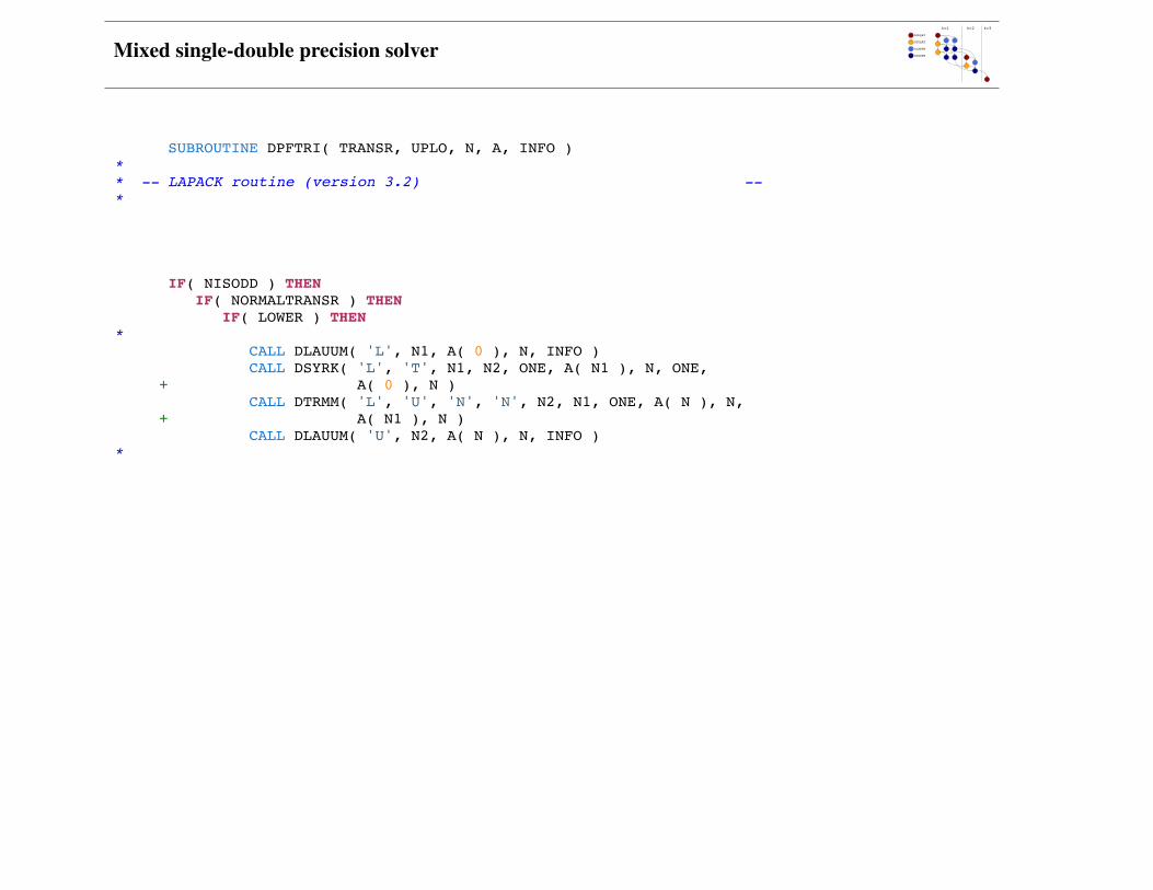
SUBROUTINE DPFTRI( TRANSR, UPLO, N, A, INFO )** -- LAPACK routine (version 3.2) --*
IF( NISODD ) THEN IF( NORMALTRANSR ) THEN IF( LOWER ) THEN* CALL DLAUUM( 'L', N1, A( 0 ), N, INFO ) CALL DSYRK( 'L', 'T', N1, N2, ONE, A( N1 ), N, ONE, + A( 0 ), N ) CALL DTRMM( 'L', 'U', 'N', 'N', N2, N1, ONE, A( N ), N, + A( N1 ), N ) CALL DLAUUM( 'U', N2, A( N ), N, INFO )*

Mixed single-double precision solver
SUBROUTINE DTFSM( TRANSR, SIDE, UPLO, TRANS, DIAG, M, N, ALPHA, A, + B, LDB )** -- LAPACK routine (version 3.2) --*
IF( MISODD ) THEN IF( NORMALTRANSR ) THEN IF( LOWER ) THEN IF( NOTRANS ) THEN CALL DTRSM( 'L', 'L', 'N', DIAG, M1, N, ALPHA, + A( 0 ), M, B, LDB ) CALL DGEMM( 'N', 'N', M2, N, M1, -ONE, A( M1 ), + M, B, LDB, ALPHA, B( M1, 0 ), LDB ) CALL DTRSM( 'L', 'U', 'T', DIAG, M2, N, ONE, + A( M ), M, B( M1, 0 ), LDB )*

Mixed single-double precision solver
Performance in Mflop/s of Cholesky Factorization/Inversion/Solution on SUN UltraSPARC IV+ computer.long real arithmetic.
0 500 1000 1500 2000 2500 3000 3500 40000
500
1000
1500
2000
2500
3000
3500Performance of Cholesky Factorization on SUN UltraSPARC IV+ computer, long real arithmetic
problem size
Mflo
p/s
PFTRF N UPFTRF N LPFTRF T UPFTRF T LPOTRF UPOTRF LPPTRF UPPTRF L
0 500 1000 1500 2000 2500 3000 3500 40000
500
1000
1500
2000
2500
3000Performance of Cholesky Inversion on SUN UltraSPARC IV+ computer, long real arithmetic
problem sizeM
flop/
s
PFTRF N UPFTRF N LPFTRF T UPFTRF T LPOTRF UPOTRF LPPTRF UPPTRF L
0 500 1000 1500 2000 2500 3000 3500 40000
500
1000
1500
2000
2500
3000Performance of Cholesky Solution on SUN UltraSPARC IV+ computer, long real arithmetic
problem size
Mflo
p/s
PFTRF N UPFTRF N LPFTRF T UPFTRF T LPOTRF UPOTRF LPPTRF UPPTRF L
Performance in Mflop/s of Cholesky Factorization/Inversion/Solution on SUN UltraSPARC IV+ computer.long complex arithmetic.
0 500 1000 1500 2000 2500 3000 3500 40000
500
1000
1500
2000
2500
3000
3500Performance of Cholesky Factorization on SUN UltraSPARC IV+ computer, long complex arithmetic
problem size
Mflo
p/s
PFTRF N UPFTRF N LPFTRF T UPFTRF T LPOTRF UPOTRF LPPTRF UPPTRF L
0 500 1000 1500 2000 2500 3000 3500 4000500
1000
1500
2000
2500
3000
3500Performance of Cholesky Inversion on SUN UltraSPARC IV+ computer, long complex arithmetic
problem size
Mflo
p/s
PFTRF N UPFTRF N LPFTRF T UPFTRF T LPOTRF UPOTRF LPPTRF UPPTRF L
0 500 1000 1500 2000 2500 3000 3500 40000
500
1000
1500
2000
2500
3000
3500Performance of Cholesky Solution on SUN UltraSPARC IV+ computer, long complex arithmetic
problem size
Mflo
p/s
PFTRF N UPFTRF N LPFTRF T UPFTRF T LPOTRF UPOTRF LPPTRF UPPTRF L

Mixed single-double precision solver
Performance in Mflop/s of Cholesky Factorization/Inversion/Solution on SGI Altix 3700, Intel Itanium 2 computer.long real arithmetic.
0 1000 2000 3000 40000
500
1000
1500
2000
2500
3000
3500
4000
4500
5000
Performance of Cholesky Factorization on SGI Altix 3700, Intel Itanium2 computer, long real arithmetic
problem size
Mflo
p/s
PFTRF N UPFTRF N LPFTRF T UPFTRF T LPOTRF UPOTRF LPPTRF UPPTRF L
0 1000 2000 3000 40000
500
1000
1500
2000
2500
3000
3500
4000
4500
5000
Performance of Cholesky Inversion on SGI Altix 3700, Intel Itanium2 computer, long real arithmetic
problem sizeM
flop/
s
PFTRF N UPFTRF N LPFTRF T UPFTRF T LPOTRF UPOTRF LPPTRF UPPTRF L
0 1000 2000 3000 40000
1000
2000
3000
4000
5000
6000Performance of Cholesky Solution on SGI Altix 3700, Intel Itanium2 computer, long real arithmetic
problem size
Mflo
p/s
PFTRF N UPFTRF N LPFTRF T UPFTRF T LPOTRF UPOTRF LPPTRF UPPTRF L
Performance in Mflop/s of Cholesky Factorization/Inversion/Solution on SGI Altix 3700, Intel Itanium 2 computer.long complex arithmetic.
0 1000 2000 3000 40000
500
1000
1500
2000
2500
3000
3500
4000
4500
5000Performance of Cholesky Factorization on SGI Altix 3700, Intel Itanium2 computer, long complex arithmetic
problem size
Mflo
p/s
PFTRF N UPFTRF N LPFTRF T UPFTRF T LPOTRF UPOTRF LPPTRF UPPTRF L
0 1000 2000 3000 40000
500
1000
1500
2000
2500
3000
3500
4000
4500
5000Performance of Cholesky Inversion on SGI Altix 3700, Intel Itanium2 computer, long complex arithmetic
problem size
Mflo
p/s
PFTRF N UPFTRF N LPFTRF T UPFTRF T LPOTRF UPOTRF LPPTRF UPPTRF L
0 1000 2000 3000 40000
500
1000
1500
2000
2500
3000
3500
4000
4500
5000Performance of Cholesky Solution on SGI Altix 3700, Intel Itanium2 computer, long complex arithmetic
problem size
Mflo
p/s
PFTRF N UPFTRF N LPFTRF T UPFTRF T LPOTRF UPOTRF LPPTRF UPPTRF L

Mixed single-double precision solver
Performance in Mflop/s of Cholesky Factorization/Inversion/Solution on ia64 Itanium computer.
0 500 1000 1500 2000 2500 3000 3500 40000
500
1000
1500
2000
2500
3000
3500
4000
4500Performance of Cholesky Factorization on ia64 Itanium computer
problem size
Mflo
p/s
PFTRF N UPFTRF N LPFTRF T UPFTRF T LPOTRF UPOTRF LPPTRF UPPTRF L
0 500 1000 1500 2000 2500 3000 3500 40000
500
1000
1500
2000
2500
3000
3500
4000
4500Performance of Cholesky Inversion on ia64 Itanium computer
problem size
Mflo
p/s
PFTRI N UPFTRI N LPFTRI T UPFTRI T LPOTRI UPOTRI LPPTRI UPPTRI L
0 500 1000 1500 2000 2500 3000 3500 40000
500
1000
1500
2000
2500
3000
3500
4000
4500Performance of Cholesky Solution on ia64 Itanium computer
problem size (nrhs=100 to 400)
Mflo
p/s
PFTRS N UPFTRS N LPFTRS T UPFTRS T LPOTRS UPOTRS LPPTRS UPPTRS L

Mixed single-double precision solver
Performance in Mflop/s of Cholesky Factorization/Inversion/Solution on SX-6 NEC computer.
0 500 1000 1500 2000 2500 3000 3500 40000
1000
2000
3000
4000
5000
6000
7000
8000Performance of Cholesky Factorization on SX−6 NEC computer
problem size
Mflo
p/s
PFTRF N UPFTRF N LPFTRF T UPFTRF T LPOTRF UPOTRF LPPTRF UPPTRF L
0 500 1000 1500 2000 2500 3000 3500 40000
1000
2000
3000
4000
5000
6000
7000
8000Performance of Cholesky Inversion on SX−6 NEC computer
problem size
Mflo
p/s
PFTRI N UPFTRI N LPFTRI T UPFTRI T LPOTRI UPOTRI LPPTRI UPPTRI L
0 500 1000 1500 2000 2500 3000 3500 40000
1000
2000
3000
4000
5000
6000
7000
8000Performance of Cholesky Solution on SX−6 NEC computer
problem size (nrhs=100 to 400)
Mflo
p/s
PFTRS N UPFTRS N LPFTRS T UPFTRS T LPOTRS UPOTRS LPPTRS UPPTRS L

Mixed single-double precision solver
Performance of Cholesky Factorization/Inversion/Solution on quad-socket quad-core Intel Tigerton computer. Weuse reference LAPACK-3.2.0 (from netlib) and MKL-10.0.1.014 multithreaded BLAS. For the solution phase,nrhs is fixed to 100 for any n. Due to time limitation, the experiment was stopped for the packed storage formatinversion at n = 4000.
0 5000 10000 15000 200000
10
20
30
40
50
60Performance of Cholesky Factorization on Intel Tigerton computer (ref. LAPACK)
problem size
Gflo
p/s
PFTRF N UPFTRF N LPFTRF T UPFTRF T LPOTRF UPOTRF LPPTRF UPPTRF L
0 5000 10000 15000 200000
5
10
15
20
25
30
35
40
45
50Performance of Cholesky Inversion on Intel Tigerton computer (ref LAPACK)
problem size
Gflo
p/s
PFTRI N UPFTRI N LPFTRI T UPFTRI T LPOTRI UPOTRI LPPTRI UPPTRI L
0 5000 10000 15000 200000
100
200
300
400
500
600
700
800Performance of Cholesky Solution on Intel Tigerton computer (ref LAPACK)
problem size (nrhs=100)
Mflo
p/s
PFTRS N UPFTRS N LPFTRS T UPFTRS T LPOTRS UPOTRS LPPTRS UPPTRS L

Mixed single-double precision solver
Performance of Cholesky Factorization/Inversion/Solution on quad-socket quad-core Intel Tigerton computer. Weuse MKL-10.0.1.014 multithreaded LAPACK and BLAS. For the solution phase, nrhs is fixed to 100 for any n.Due to time limitation, the experiment was stopped for the packed storage format inversion at n = 4000.
0 5000 10000 15000 200000
10
20
30
40
50
60
70
80
90
100Performance of Cholesky Factorization on Intel Tigerton computer (MKL)
problem size
Gflo
p/s
PFTRF N UPFTRF N LPFTRF T UPFTRF T LPOTRF UPOTRF LPPTRF UPPTRF L
0 5000 10000 15000 200000
5
10
15
20
25
30
35
40
45
50Performance of Cholesky Inversion on Intel Tigerton computer (MKL)
problem size
Gflo
p/s
PFTRI N UPFTRI N LPFTRI T UPFTRI T LPOTRI UPOTRI LPPTRI UPPTRI L
0 5000 10000 15000 200000
20
40
60
80
100
120
140
160
180
200Performance of Cholesky Solution on Intel Tigerton computer (MKL)
problem size (nrhs=100)
Mflo
p/s
PFTRS N UPFTRS N LPFTRS T UPFTRS T LPOTRS UPOTRS LPPTRS UPPTRS L

Mixed single-double precision solver
Performance in Gflop/s of Cholesky Factorization on IBM Power 4 (left) and SUN UltraSPARC-IV (right) com-puter with a different number of Processors, testing the SMP Parallelism. The implementation of PPTRF of sunperfdoes not show any SMP parallelism. UPLO = ’L’. N = 5,000 (strong scaling experiment).
0 5 10 150
5
10
15
20
25
30
35
40Scalabilty of Cholesky Factorization on an IBM Power 4 computer
number of processors
Gflo
p/s
PFTRF N LPOTRF LPPTRF L
0 5 10 150
5
10
15
20
25
30Scalabilty of Cholesky Factorization on a SUN UltraSPARC−IV computer
number of processors
Gflo
p/s
PFTRF N LPOTRF LPPTRF L

Mixed single-double precision solver
Julien Langou, University of Colorado Denver.
Mixed single-double precision solverWednesday April 1st, 2008.
1. Mixed single-double precision solver2. Rectangular Full Packed Format3. Communication optimal algorithm

Mixed single-double precision solver
For more information:
• Alfredo Buttari, Julien Langou, Jakub Kurzak and Jack Dongarra. A class of parallel tiled linear algebraalgorithms for multicore architectures. Parallel Computing, 35:38-53, 2009.
• Alfredo Buttari, Julien Langou, Jakub Kurzak and Jack Dongarra. Parallel tiled QR factorization for multicorearchitectures. Concurrency Computat.: Pract. Exper., 20(13):1573-1590, 2008.
• James W. Demmel, Laura Grigori, Mark F. Hoemmen, and Julien Langou. Communication-optimal paralleland sequential QR and LU factorizations. arXiv:0808.2664.
• James W. Demmel, Laura Grigori, Mark F. Hoemmen, and Julien Langou. Implementing Communication-Optimal Parallel and Sequential QR Factorizations. arXiv:0809.2407.

Mixed single-double precision solver
1. TSQR: Tall Skinny QR
2. CAQR: Communication Avoiding QR

Mixed single-double precision solver
1. TSQR: Tall Skinny QR
2. CAQR: Communication Avoiding QR

Mixed single-double precision solver
AllReduceAlgorithms:Applica4ontoHouseholderQRFactoriza4on
JimDemmel,UniversityofCalifornia,Berkeley;LauraGrigori,INRIA,France;MarkHoemmen,UniversityofCalifornia,Berkeley;JulienLangou,UniversityofColorado,Denver

Mixed single-double precision solver
ReduceAlgorithms:Introduc4onTheQRfactoriza4onofalongandskinnymatrixwithitsdatapar44onedver4callyacrossseveralprocessorsarisesinawiderangeofapplica4ons.
A1
A2
A3
Q1
Q2
Q3
R
Input:Aisblockdistributedbyrows
Output:QisblockdistributedbyrowsRisglobal

Mixed single-double precision solver
ReduceAlgorithms:Introduc4onExampleofapplica3ons:
a) inlinearleastsquaresproblemswhichthenumberofequa4onsisextremelylargerthanthenumberofunknowns

Mixed single-double precision solver
ReduceAlgorithms:Introduc4onExampleofapplica3ons:
a) inlinearleastsquaresproblemswhichthenumberofequa4onsisextremelylargerthanthenumberofunknowns
b) inblockitera4vemethods(itera4vemethodswithmul4pleright‐handsidesoritera4veeigenvaluesolvers)
Mixed single-double precision solver
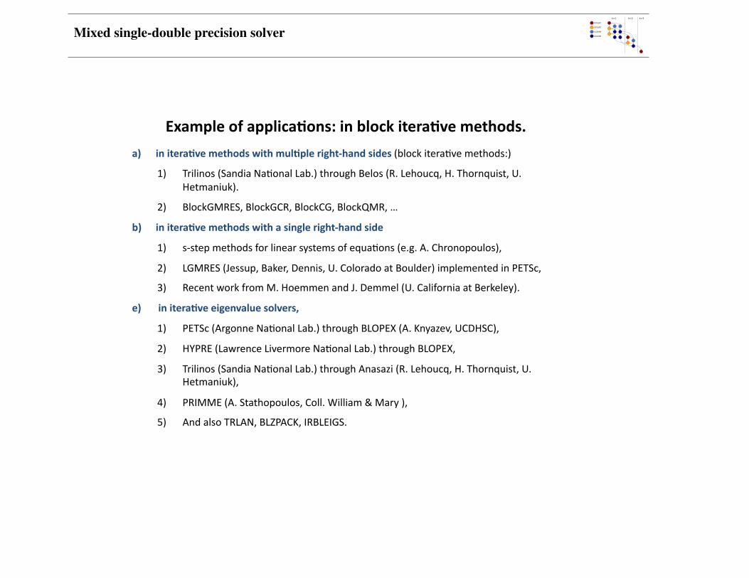
Exampleofapplica3ons:inblockitera3vemethods.
a) initera3vemethodswithmul3pleright‐handsides(blockitera4vemethods:)
1) Trilinos(SandiaNa4onalLab.)throughBelos(R.Lehoucq,H.Thornquist,U.Hetmaniuk).
2) BlockGMRES,BlockGCR,BlockCG,BlockQMR,…
b) initera3vemethodswithasingleright‐handside
1) s‐stepmethodsforlinearsystemsofequa4ons(e.g.A.Chronopoulos),
2) LGMRES(Jessup,Baker,Dennis,U.ColoradoatBoulder)implementedinPETSc,
3) RecentworkfromM.HoemmenandJ.Demmel(U.CaliforniaatBerkeley).
e) initera3veeigenvaluesolvers,
1) PETSc(ArgonneNa4onalLab.)throughBLOPEX(A.Knyazev,UCDHSC),
2) HYPRE(LawrenceLivermoreNa4onalLab.)throughBLOPEX,
3) Trilinos(SandiaNa4onalLab.)throughAnasazi(R.Lehoucq,H.Thornquist,U.Hetmaniuk),
4) PRIMME(A.Stathopoulos,Coll.William&Mary),
5) AndalsoTRLAN,BLZPACK,IRBLEIGS.

Mixed single-double precision solver
ReduceAlgorithms:Introduc4onExampleofapplica3ons:
a) inlinearleastsquaresproblemswhichthenumberofequa4onsisextremelylargerthanthenumberofunknowns
b) inblockitera4vemethods(itera4vemethodswithmul4pleright‐handsidesoritera4veeigenvaluesolvers)
c) indenselargeandmoresquareQRfactoriza4onwheretheyareusedasthepanelfactoriza4onstep

Mixed single-double precision solver
BlockedLUandQRalgorithms(LAPACK)
‐
lu( )
dgeK2
dtrsm(+dswp)
dgemm
\
L
U
A(1)
A(2)L
U
‐
qr( )
dgeqf2+dlarQ
dlarR
V
R
A(1)
A(2)V
R
LAPACKblockLU(right‐looking):dgetrf LAPACKblockQR(right‐looking):dgeqrf
Upd
ateofth
eremainingsub
matrix
Pane
lfactoriza4
on

Mixed single-double precision solver
BlockedLUandQRalgorithms(LAPACK)
‐
lu( )
dgeK2
dtrsm(+dswp)
dgemm
\
L
U
A(1)
A(2)L
U
LAPACKblockLU(right‐looking):dgetrf
Upd
ateofth
eremainingsub
matrix
Pane
lfactoriza4
on
Latencybounded:morethannbAllReduceforn*nb2ops
CPU‐bandwidthbounded:thebulkofthecomputa4on:n*n*nbopshighlyparalleliable,efficientandsaclable.

Mixed single-double precision solver
Paralleliza3onofLUandQR.
Parallelizetheupdate:• Easyanddoneinanyreasonablesoeware.• Thisisthe2/3n3termintheFLOPscount.• CanbedoneefficientlywithLAPACK+mul4threadedBLAS
‐
dgemm
‐
lu( )
dgeK2
dtrsm(+dswp)
dgemm
\
L
U
A(1)
A(2)L
U

Mixed single-double precision solver
Paralleliza3onofLUandQR.
Parallelizetheupdate:• Easyanddoneinanyreasonablesoeware.• Thisisthe2/3n3termintheFLOPscount.• CanbedoneefficientlywithLAPACK+mul4threadedBLAS
Parallelizethepanelfactoriza3on:• Notanop4oninmul4corecontext(p<16)• Seee.g.ScaLAPACKorHPLbuts4llbyfartheslowestandthebojleneckofthecomputa4on.
Hidethepanelfactoriza3on:• Lookahead(seee.g.HighPerformanceLINPACK)• DynamicScheduling
lu( )
dgeK2
‐
dgemm
lu( )
dgeK2

Mixed single-double precision solver
Hidingthepanelfactoriza4onwithdynamicscheduling.
TimeCourtesyfromAlfredoBujari,UTennessee

Mixed single-double precision solver
Whataboutstrongscalability?

Mixed single-double precision solver
Whataboutstrongscalability?N=1536
NB=64
procs=16
CourtesyfromJakubKurzak,UTennessee

Mixed single-double precision solver
Whataboutstrongscalability?N=1536
NB=64
procs=16
Wecannothidethepanelfactoriza4onintheMM,actuallyitistheMMsthatarehiddenbythepanelfactoriza4ons!
CourtesyfromJakubKurzak,UTennessee

Mixed single-double precision solver
Whataboutstrongscalability?N=1536
NB=64
procs=16
Wecannothidethepanelfactoriza4on(n2)withtheMM(n3),actuallyitistheMMsthatarehiddenbythepanelfactoriza4ons!
NEEDFORNEWMATHEMATICALALGORITHMS
CourtesyfromJakubKurzak,UTennessee

Mixed single-double precision solver
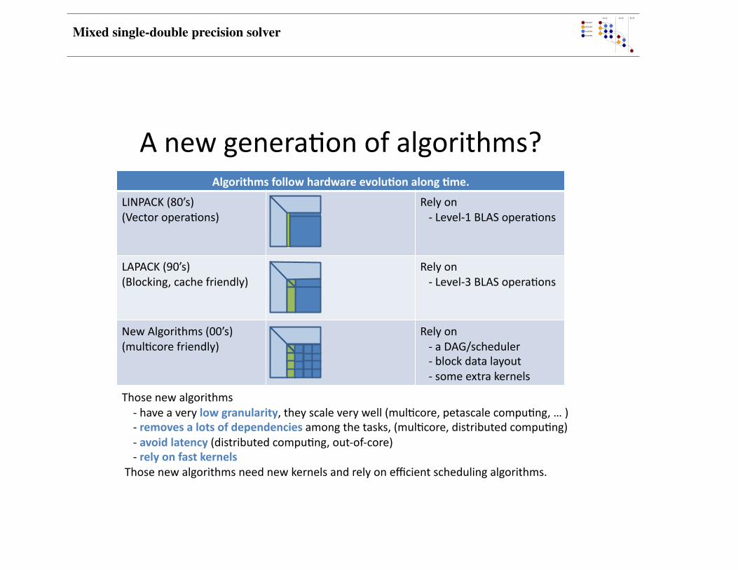
Anewgenera4onofalgorithms?Algorithmsfollowhardwareevolu3onalong3me.
LINPACK(80’s)(Vectoropera4ons)
Relyon‐Level‐1BLASopera4ons
LAPACK(90’s)(Blocking,cachefriendly)
Relyon‐Level‐3BLASopera4ons
Mixed single-double precision solver
Anewgenera4onofalgorithms?Algorithmsfollowhardwareevolu3onalong3me.
LINPACK(80’s)(Vectoropera4ons)
Relyon‐Level‐1BLASopera4ons
LAPACK(90’s)(Blocking,cachefriendly)
Relyon‐Level‐3BLASopera4ons
NewAlgorithms(00’s)(mul4corefriendly)
Relyon‐aDAG/scheduler‐blockdatalayout‐someextrakernels
Thosenewalgorithms‐haveaverylowgranularity,theyscaleverywell(mul4core,petascalecompu4ng,…)‐removesalotsofdependenciesamongthetasks,(mul4core,distributedcompu4ng)‐avoidlatency(distributedcompu4ng,out‐of‐core)‐relyonfastkernelsThosenewalgorithmsneednewkernelsandrelyonefficientschedulingalgorithms.

Mixed single-double precision solver
2005‐2007:Newalgorithmsbasedon2Dpar44onning:
– UTexas(vandeGeijn):SYRK,CHOL(mul4core),LU,QR(out‐of‐core)– UTennessee(Dongarra):CHOL(mul4core)– HPC2N(Kågström)/IBM(Gustavson):Chol(Distributed)
– UCBerkeley(Demmel)/INRIA(Grigori):LU/QR(distributed)– UCDenver(Langou):LU/QR(distributed)
A3rdrevolu4onfordenselinearalgebra?

Mixed single-double precision solver
ReduceAlgorithms:Introduc4onExampleofapplica3ons:
a) inblockitera4vemethods(itera4vemethodswithmul4pleright‐handsidesoritera4veeigenvaluesolvers),
b) indenselargeandmoresquareQRfactoriza4onwheretheyareusedasthepanelfactoriza4onstep,ormoresimply
c) inlinearleastsquaresproblemswhichthenumberofequa4onsisextremelylargerthanthenumberofunknowns.
Themaincharacteris3csofthosethreeexamplesarethat
a) thereisonlyonecolumnofprocessorsinvolvedbutseveralprocessorrows,
b) allthedataisknownfromthebeginning,
c) andthematrixisdense.
VariousmethodsalreadyexisttoperformtheQRfactoriza4onofsuchmatrices:
a) Gram‐Schmidt(mgs(row),cgs),
b) Householder(qr2,qrf),
c) orCholeskyQR.
Wepresentanewmethod:
AllreduceHouseholder(rhh_qr3,rhh_qrf).

Mixed single-double precision solver
TheCholeskyQRAlgorithm
chol( )
/
Ci AiT Ai
AiQi
CR
R
SYRK: C:=ATA (mn2)
CHOL: R:=chol(C) (n3/3)
TRSM: Q:=A/R (mn2)

Mixed single-double precision solver
Bibligraphy
• A.StathopoulosandK.Wu,Ablockorthogonaliza4onprocedurewithconstantsynchroniza4onrequirements,SIAMJournalonScien0ficCompu0ng,23(6):2165‐2182,2002.
• Popularizedbyitera4veeigensolverlibraries:
1) PETSc(ArgonneNa4onalLab.)throughBLOPEX(A.Knyazev,UCDHSC),
2) HYPRE(LawrenceLivermoreNa4onalLab.)throughBLOPEX,
3) Trilinos(SandiaNa4onalLab.)throughAnasazi(R.Lehoucq,H.Thornquist,U.Hetmaniuk),
4) PRIMME(A.Stathopoulos,Coll.William&Mary).

Mixed single-double precision solver
ParalleldistributedCholeskyQRTheCholeskyQRmethodintheparalleldistributedcontextcanbedescribedasfollows:
+
chol( )
/
+ +
1.
2.
3‐4.
5.
C C1 C2 C3 C4
Ci AiT Ai
AiQi
CR
R
1:SYRK: C:=ATA (mn2)
2:MPI_Reduce: C:=sumprocsC (onproc0)
3:CHOL: R:=chol(C) (n3/3)
4:MPI_Bdcast BroadcasttheRfactoronproc0
toalltheotherprocessors
5:TRSM: Q:=A/R (mn2)

Mixed single-double precision solver
Efficientenough?
#ofprocs
cholqr cgs mgs(row) qrf mgs
1 489.2 (1.02) 134.1 (3.73) 73.5 (6.81) 39.1 (12.78) 56.18 (8.90)
2 467.3 (0.54) 78.9 (3.17) 39.0 (6.41) 22.3 (11.21) 31.21 (8.01)
4 466.4 (0.27) 71.3 (1.75) 38.7 (3.23) 22.2 (5.63) 29.58 (4.23)
8 434.0 (0.14) 67.4 (0.93) 36.7 (1.70) 20.8 (3.01) 21.15 (2.96)
16 359.2 (0.09) 54.2 (0.58) 31.6 (0.99) 18.3 (1.71) 14.44 (2.16)
32 197.8 (0.08) 41.9 (0.37) 29.0 (0.54) 15.8 (0.99) 8.38 (1.87)
MFLOP/sec/proc
Timeinsec
Inthisexperiment,wefixtheproblem:m=100,000andn=50.
Performance(M
FLOP/sec/proc)
Time(sec)
#ofprocs#ofprocs

Mixed single-double precision solver
Simpleenough?
intcholeskyqr_A_v0(intmloc,intn,double*A,intlda,double*R,intldr,MPI_Commmpi_comm){
intinfo;cblas_dsyrk(CblasColMajor,CblasUpper,CblasTrans,n,mloc, 1.0e+00,A,lda,0e+00,R,ldr);MPI_Allreduce(MPI_IN_PLACE,R,n*n,MPI_DOUBLE,MPI_SUM,mpi_comm);lapack_dpotrf(lapack_upper,n,R,ldr,&info);cblas_dtrsm(CblasColMajor,CblasRight,CblasUpper,CblasNoTrans,CblasNonUnit, mloc,n,1.0e+00,R,ldr,A,lda);return0;
}
(…and,OK,youmightwanttoaddanMPIuserdefineddatatypetosendonlytheupperpartofR)
+
chol( )
\
+ +
1.
2.
3‐4.
5.
C C1 C2 C3 C4
Ci AiT
Ai
AiQi
CR
R

Mixed single-double precision solver
Stableenough?
1.00E‐161.00E‐141.00E‐121.00E‐101.00E‐081.00E‐061.00E‐041.00E‐021.00E+00
1.00E+001.00E+021.00E+041.00E+061.00E+081.00E+101.00E+121.00E+14
cholqr
cgs
mgs
Householder
1.00E‐16
1.00E‐15
1.00E‐14
1.00E+001.00E+021.00E+041.00E+061.00E+081.00E+101.00E+121.00E+14
cholqr
cgs
mgs
Householder
κ2(A)
κ2(A)
||A–QR|| 2/||A|| 2
||I–Q
T Q|| 2
m=100,n=50

Mixed single-double precision solver
ParalleldistributedCholeskyQRTheCholeskyQRmethodintheparalleldistributedcontextcanbedescribedasfollows:
+
chol( )
/
+ +
1.
2.
3‐4.
5.
C C1 C2 C3 C4
Ci AiT Ai
AiQi
CR
R
1:SYRK: C:=ATA (mn2)
2:MPI_Reduce: C:=sumprocsC (onproc0)
3:CHOL: R:=chol(C) (n3/3)
4:MPI_Bdcast BroadcasttheRfactoronproc0
toalltheotherprocessors
5:TRSM: Q:=A/R (mn2)
Thismethodisextremelyfast.Fortworeasons:1. first,thereisonlyoneortwocommunica3onsphase,2. second,thelocalcomputa3onsareperformedwithfastopera3ons.
Anotheradvantageofthismethodisthattheresul4ngcodeisexactlyfourlines,3. sothemethodissimpleandreliesheavilyonotherlibraries.
Despiteallthoseadvantages,4. thismethodishighlyunstable.

Mixed single-double precision solver
ReduceAlgorithmsThegather‐scajervariantofouralgorithmcanbe
summarizedasfollows:
1. performlocalQRfactoriza4onofthematrixA
2. gatherthepRfactorsonprocessor03. performaQRfactoriza4onofalltheRputthe
onesontopoftheothers,theRfactorobtainedistheRfactor
4. scajerthetheQfactorsfromprocessor0toalltheprocessors
5. mul4plylocallythetwoQfactorstogether,done.
*
1.
2‐3‐4.
5.
Qi(0)Ri
Ai
R R1
R2
R3
R4QW4
QW3
QW2
QW1
QWi
Qi(0)Q
qr(
qr( )
)

Mixed single-double precision solver
ReduceAlgorithms
• Thisisthescajer‐gatherversionofouralgorithm.
• Thisvariantisnotveryefficientfortworeasons:– firstthecommunica4onphases2and4arehighlyinvolving
processor0;– secondthecostofstep3isp/3*n3,socangetprohibi4vefor
largep.
• NotethattheCholeskyQRalgorithmcanalsobeimplementedinascajer‐gatherwaybutreduce‐broadcast.Thisleadsnaturallytothealgorithmpresentedbelowwhereareduce‐broadcastversionofthepreviousalgorithmisdescribed.Thiswillbeourfinalalgorithm.
Mixed single-double precision solver
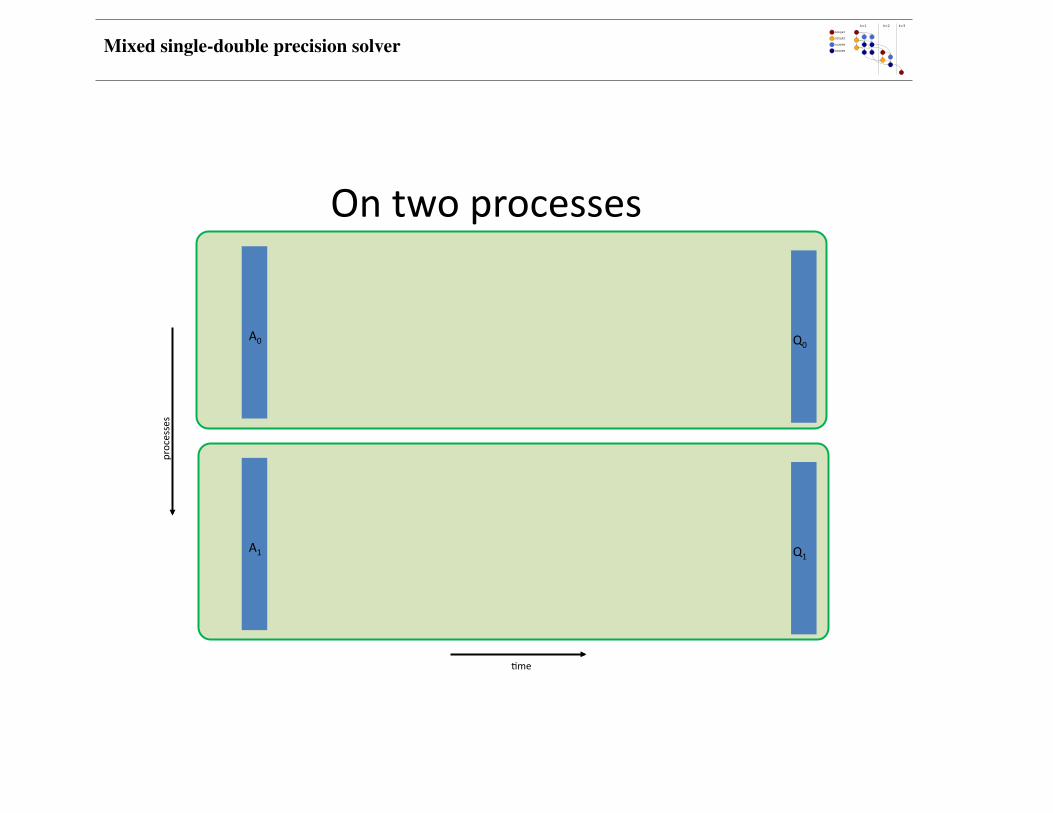
Ontwoprocesses
A0 Q0
A1 Q1
processes
4me

Mixed single-double precision solver
OntwoprocessesR0(0)( , )QR( )
A0 V0(0)
R1(0)( , )QR( )
A1 V1(0)
processes
4me

Mixed single-double precision solver
OntwoprocessesR0(0)( , )QR( )
A0 V0(0)
)R0(0)
R1(0)
R1(0)( , )QR( )
A1 V1(0)
processes
4me
(

Mixed single-double precision solver
OntwoprocessesR0(0)( , )QR( )
A0 V0(0)
R0(1)( , )QR( )R0(0)
R1(0)
V0(1)
V1(1)
R1(0)( , )QR( )
A1 V1(0)
processes
4me

Mixed single-double precision solver
OntwoprocessesR0(0)( , )QR( )
A0 V0(0)
R0(1)( , )QR( )R0(0)
R1(0)
V0(1)
V1(1)
InApply( to )V0(1)
0nV1(1)
Q0(1)
Q1(1)
R1(0)( , )QR( )
A1 V1(0)
processes
4me

Mixed single-double precision solver
OntwoprocessesR0(0)( , )QR( )
A0 V0(0)
R0(1)( , )QR( )R0(0)
R1(0)
V0(1)
V1(1)
InApply( to )V0(1)
0nV1(1)
Q0(1)
Q1(1)
Q0(1)
R1(0)( , )QR( )
A1 V1(0)
processes
4me
Q1(1)

Mixed single-double precision solver
OntwoprocessesR0(0)( , )QR( )
A0 V0(0)
R0(1)( , )QR( )R0(0)
R1(0)
V0(1)
V1(1)
InApply( to )V0(1)
0nV1(1)
Q0(1)
Q1(1)
Apply( to )0n
V0(0)
Q0(1)
Q0
R1(0)( , )QR( )
A1 V1(0)
Apply( to )
V1(0)
Q1(1)
Q1
processes
4me
0n

Mixed single-double precision solver
Thebigpicture….
A1
A2
A3
A4
A5
A6
Q0
Q4
Q1
Q5
Q6
Q3
Q2
R
R
R
R
R
R
R
A QR4me
processes
A0

Mixed single-double precision solver
Thebigpicture….
A1
A2
A3
A4
A5
A6
4me
processes
communica3on
computa3on
A0

Mixed single-double precision solver
Thebigpicture….
A1
A2
A3
A4
A5
A6
4me
processes
communica3on
computa3on
A0

Mixed single-double precision solver
Thebigpicture….
A1
A2
A3
A4
A5
A6
4me
processes
communica3on
computa3on
A0

Mixed single-double precision solver
Thebigpicture….
A1
A2
A3
A4
A5
A6
4me
processes
communica3on
computa3on
A0

Mixed single-double precision solver
Thebigpicture….
A1
A2
A3
A4
A5
A6
4me
processes
communica3on
computa3on
A0

Mixed single-double precision solver
Thebigpicture….
A1
A2
A3
A4
A5
A6
4me
processes
communica3on
computa3on
A0

Mixed single-double precision solver
Thebigpicture….
A1
A2
A3
A4
A5
A6
4me
processes
communica3on
computa3on
A0

Mixed single-double precision solver
Thebigpicture….
A1
A2
A3
A4
A5
A6
4me
processes
communica3on
computa3on
A0

Mixed single-double precision solver
Thebigpicture….
A1
A2
A3
A4
A5
A6
Q0
Q4
Q1
Q5
Q6
Q3
Q2
R
R
R
R
R
R
R
4me
processes
communica3on
computa3on
A0

Mixed single-double precision solver
Latencybutalsopossibilityoffastpanelfactoriza4on.
• DGEQR3istherecursivealgorithm(seeElmrothandGustavson,2000),DGEQRFandDGEQR2aretheLAPACKrou4nes.
• TimesincludeQRandDLARFT.
• RunonPen4umIII.
QRfactoriza3onandconstruc3onofTm=10,000
PerfinMFLOP/sec(Timesinsec)
n DGEQR3 DGEQRF DGEQR2
50 173.6 (0.29) 65.0 (0.77) 64.6 (0.77)
100 240.5 (0.83) 62.6 (3.17) 65.3 (3.04)
150 277.9 (1.60) 81.6 (5.46) 64.2 (6.94)
200 312.5 (2.53) 111.3 (7.09) 65.9 (11.98)
m=1000,000,thexaxisisn
MFLOP/sec
Mixed single-double precision solver
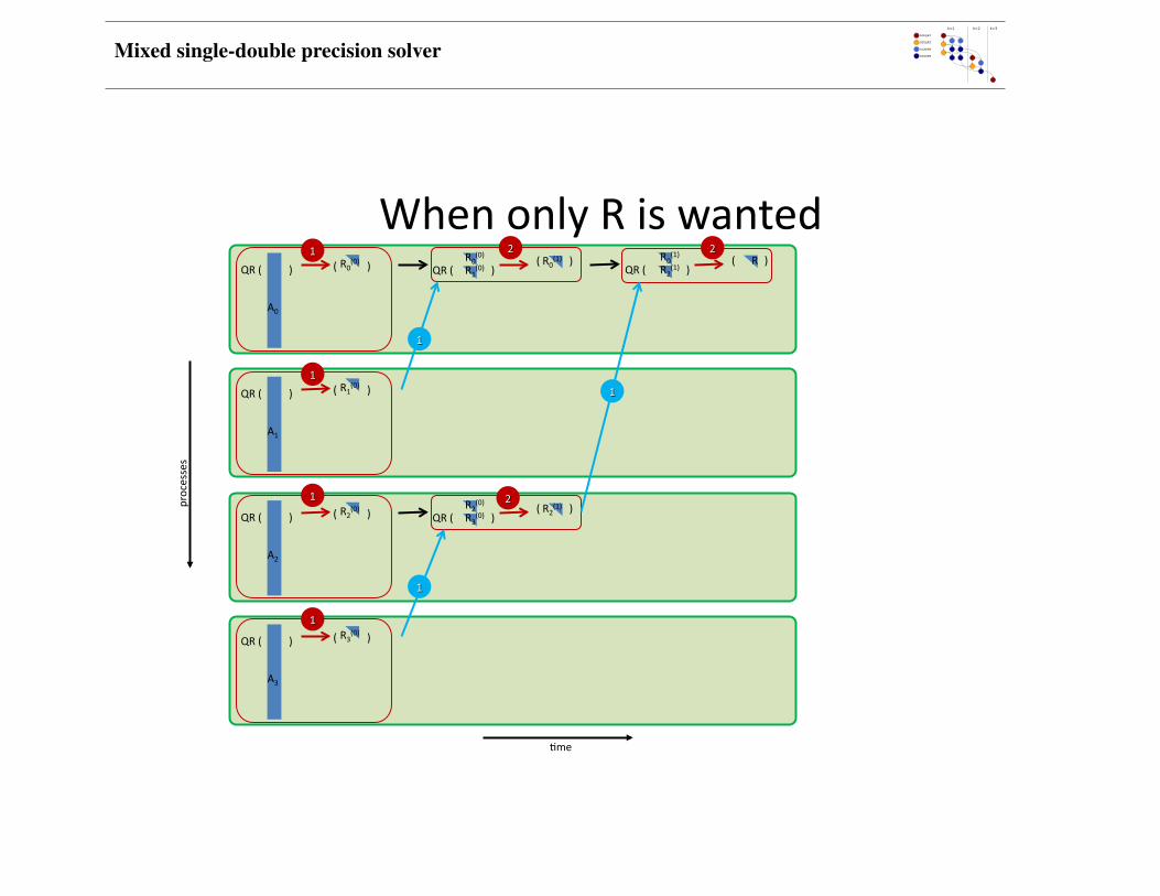
WhenonlyRiswantedprocesses
4me
R0(0)( )QR( )
A0
R0(1)( )QR( )
R0(0)R1(0)
R1(0)( )QR( )
A1
R2(0)( )QR( )
A2
R2(1)( )QR( )
R2(0)R3(0)
R3(0)( )QR( )
A3
R( )QR( )
R0(1)R2(1)

Mixed single-double precision solver
WhenonlyRiswanted:TheMPI_Allreduce
InthecasewhereonlyRiswanted,insteadofconstruc4ngourowntree,onecansimplyuseMPI_Allreducewithauserdefinedopera4on.Theopera4onwegivetoMPIisbasicallytheAlgorithm2.Itperformstheopera4on:
Thisbinaryopera4onisassocia3veandthisisallMPIneedstouseauser‐definedopera4ononauser‐defineddatatype.Moreover,ifwechangethesignsoftheelementsofRsothatthediagonalofRholdsposi4veelementsthenthebinaryopera4onRfactorbecomescommuta3ve.
Thecodebecomestwolines:
lapack_dgeqrf( mloc, n, A, lda, tau, &dlwork, lwork, &info );
MPI_Allreduce( MPI_IN_PLACE, A, 1, MPI_UPPER,
LILA_MPIOP_QR_UPPER, mpi_comm);
QR ( )R1R2
R

Mixed single-double precision solver
Doesitwork?• TheexperimentsareperformedonthebeowulfclusterattheUniversityofColoradoatDenver.The
clusterismadeof35bi‐proPen4umIII(900MHz)connectedwithDolphininterconnect.• Numberofopera4onsistakenas2mn2forallthemethods
• TheblocksizeusedinScaLAPACKis32.
• ThecodeiswrijeninC,useMPI(mpich‐2.1),LAPACK(3.1.1),BLAS(goto‐1.10),theLAPACKCwrappers(hjp://icl.cs.utk.edu/~delmas/lapwrapmw.htm)andtheBLASCwrappers(hjp://www.netlib.org/blas/blast‐forum/cblas.tgz)
• Thecodeshasbeentestedinvariousconfigura4onandhaveneverfailedtoproduceacorrectanswer,releasingthosecodesisintheagenda
FLOPs(total)forRonly FLOPs(total)forQandR
CholeskyQR mn2+n3/3 2mn2+n3/3
Gram‐Schmidt 2mn2 2mn2
Householder 2mn2‐2/3n3 4mn2‐4/3n3
AllreduceHH (2mn2‐2/3n3)+2/3n3p (4mn2‐4/3n3)+4/3n3p
» Numberofopera3onsistakenas2mn2forallthemethods

Mixed single-double precision solver
QandR:Strongscalability• Inthisexperiment,wefixthe
problem:m=100,000andn=50.Thenweincreasethenumberofprocessors.
• Oncemorethealgorithmrhh_qr3isthesecondbehindCholeskyQR.Notethatrhh_qr3isincondionnallystablewhilethestabilityofCholeskyQRdependsonthesquareofthecondi4onnumberoftheini4almatrix.
#ofprocs
cholqr rhh_qr3 cgs mgs(row) rhh_qrf qrf qr2
1 489.2 (1.02) 120.0 (4.17) 134.1 (3.73) 73.5 (6.81) 51.9 (9.64) 39.1 (12.78) 34.3 (14.60)
2 467.3 (0.54) 100.8 (2.48) 78.9 (3.17) 39.0 (6.41) 31.2 (8.02) 22.3 (11.21) 20.2 (12.53)
4 466.4 (0.27) 97.9 (1.28) 71.3 (1.75) 38.7 (3.23) 31.0 (4.03) 22.2 (5.63) 18.8 (6.66)
8 434.0 (0.14) 95.9 (0.65) 67.4 (0.93) 36.7 (1.70) 34.0 (1.84) 20.8 (3.01) 17.7 (3.54)
16 359.2 (0.09) 103.8 (0.30) 54.2 (0.58) 31.6 (0.99) 27.8 (1.12) 18.3 (1.71) 16.3 (1.91)
32 197.8 (0.08) 84.9 (0.18) 41.9 (0.37) 29.0 (0.54) 33.3 (0.47) 15.8 (0.99) 14.5 (1.08)
#procs
MFLOP/sec/proc
MFLOP/sec/proc Timeinsec

Mixed single-double precision solver
QandR:Weakscalabilitywithrespecttom• Wefixthelocalsizetobemloc=100,000
andn=50.Whenweincreasethenumberofprocessors,theglobalmgrowspropor4onally.
• rhh_qr3istheAllreducealgorithmwithrecursivepanelfactoriza4on,rhh_qrfisthesamewithLAPACKHouseholderQR.Weseetheobviousbenefitofusingrecursion.Seeaswell(6).qr2andqrfcorrespondtotheScaLAPACKHouseholderQRfactoriza4onrou4nes.
#ofprocs
cholqr rhh_qr3 Cgs mgs(row) rhh_qrf qrf qr2
1 489.2 (1.02) 121.2 (4.13) 135.7 (3.69) 70.2 (7.13) 51.9 (9.64) 39.8 (12.56) 35.1 (14.23)
2 466.9 (1.07) 102.3 (4.89) 84.4 (5.93) 35.6 (14.04) 27.7 (18.06) 20.9 (23.87) 20.2 (24.80)
4 454.1 (1.10) 96.7 (5.17) 67.2 (7.44) 41.4 (12.09) 32.3 (15.48) 20.6 (24.28) 18.3 (27.29)
8 458.7 (1.09) 96.2 (5.20) 67.1 (7.46) 33.2 (15.06) 28.3 (17.67) 20.5 (24.43) 17.8 (28.07)
16 451.3 (1.11) 94.8 (5.27) 67.2 (7.45) 33.3 (15.04) 27.4 (18.22) 20.0 (24.95) 17.2 (29.10)
32 442.1 (1.13) 94.6 (5.29) 62.8 (7.97) 32.5 (15.38) 26.5 (18.84) 19.8 (25.27) 16.9 (29.61)
64 414.9 (1.21) 93.0 (5.38) 62.8 (7.96) 32.3 (15.46) 27.0 (18.53) 19.4 (25.79) 16.6 (30.13)
#procs
MFLOP/sec/proc
MFLOP/sec/proc Timeinsec

Mixed single-double precision solver
QandR:Weakscalabilitywithrespectton• Wefixtheglobalsize
m=100,000andthenweincreasenassqrt(p)sothattheworkloadmn2perprocessorremainsconstant.
• Duetobejerperformanceinthelocalfactoriza4onorSYRK,CholeskyQR,rhh_q3andrhh_qrfexhibitincreasingperformanceatthebeginningun4lthen3comesintoplay
#ofprocs
cholqr rhh_qr3 cgs mgs(row) rhh_qrf qrf qr2
1 490.7 (1.02) 120.8 (4.14) 134.0 (3.73) 69.7 (7.17) 51.7 (9.68) 39.6 (12.63) 39.9 (14.31)
2 510.2 (0.99) 126.0 (4.00) 78.6 (6.41) 40.1 (12.56) 32.1 (15.71) 25.4 (19.88) 19.0 (26.56)
4 541.1 (0.92) 149.4 (3.35) 75.6 (6.62) 39.1 (12.78) 31.1 (16.07) 25.5 (19.59) 18.9 (26.48)
8 540.2 (0.92) 173.8 (2.86) 72.3 (6.87) 38.5 (12.89) 43.6 (11.41) 27.8 (17.85) 20.2 (24.58)
16 501.5 (1.00) 195.2 (2.56) 66.8 (7.48) 38.4 (13.02) 51.3 (9.75) 28.9 (17.29) 19.3 (25.87)
32 379.2 (1.32) 177.4 (2.82) 59.8 (8.37) 36.2 (13.84) 61.4 (8.15) 29.5 (16.95) 19.3 (25.92)
64 266.4 (1.88) 83.9 (5.96) 32.3 (15.46) 36.1 (13.84) 52.9 (9.46) 28.2 (17.74) 18.4 (27.13)
MFLOP/sec/proc
#procs(n)MFLOP/sec/proc Timeinsec
n3effect

Mixed single-double precision solver
Ronly:Strongscalability• Inthisexperiment,wefixthe
problem:m=100,000andn=50.Thenweincreasethenumberofprocessors.
#ofprocs
cholqr rhh_qr3 cgs mgs(row) rhh_qrf qrf qr2
1 1099.046 (0.45) 147.6 (3.38) 139.309 (3.58) 73.5 (6.81) 69.049 (7.24) 69.108 (7.23) 68.782 (7.27)
2 1067.856 (0.23) 123.424 (2.02) 78.649 (3.17) 39.0 (6.41) 41.837 (5.97) 38.008 (6.57) 40.782 (6.13)
4 1034.203 (0.12) 116.774 (1.07) 71.101 (1.76) 38.7 (3.23) 39.295 (3.18) 36.263 (3.44) 36.046 (3.47)
8 876.724 (0.07) 119.856 (0.52) 66.513 (0.94) 36.7 (1.70) 37.397 (1.67) 35.313 (1.77) 34.081 (1.83)
16 619.02 (0.05) 129.808 (0.24) 53.352 (0.59) 31.6 (0.99) 33.581 (0.93) 31.339 (0.99) 31.697 (0.98)
32 468.332 (0.03) 95.607 (0.16) 42.276 (0.37) 29.0 (0.54) 37.226 (0.42) 25.695 (0.60) 25.971 (0.60)
64 195.885 (0.04) 77.084 (0.10) 25.89 (0.30) 22.8 (0.34) 36.126 (0.22) 17.746 (0.44) 17.725 (0.44)
#procs
MFLOP/sec/proc
MFLOP/sec/proc Timeinsec

Mixed single-double precision solver
Ronly:Weakscalabilitywithrespecttom• Wefixthelocalsizetobemloc=100,000
andn=50.Whenweincreasethenumberofprocessors,theglobalmgrowspropor4onally.
#ofprocs
cholqr rhh_qr3 cgs mgs(row) rhh_qrf qrf qr2
1 1098.7 (0.45) 145.4 (3.43) 138.2 (3.61) 70.2 (7.13) 70.6 (7.07) 68.7 (7.26) 69.1 (7.22)
2 1048.3 (0.47) 124.3 (4.02) 70.3 (7.11) 35.6 (14.04) 43.1 (11.59) 35.8 (13.95) 36.3 (13.76)
4 1044.0 (0.47) 116.5 (4.29) 82.0 (6.09) 41.4 (12.09) 35.8 (13.94) 36.3 (13.74) 34.7 (14.40)
8 993.9 (0.50) 116.2 (4.30) 66.3 (7.53) 33.2 (15.06) 35.1 (14.21) 35.5 (14.05) 33.8 (14.75)
16 918.7 (0.54) 115.2 (4.33) 64.1 (7.79) 33.3 (15.04) 34.0 (14.66) 33.4 (14.94) 33.0 (15.11)
32 950.7 (0.52) 112.9 (4.42) 63.6 (7.85) 32.5 (15.38) 33.4 (14.95) 33.3 (15.01) 32.9 (15.19)
64 764.6 (0.65) 112.3 (4.45) 62.7 (7.96) 32.3 (15.46) 34.0 (14.66) 32.6 (15.33) 32.3 (15.46)
#procs
MFLOP/sec/proc
MFLOP/sec/proc Timeinsec

Mixed single-double precision solver
QandR:Strongscalability
0
100
200
300
400
500
600
700
800
32 64 128 256
ReduceHH(QR3)
ReduceHH(QRF)
ScaLAPACKQRF
ScaLAPACKQR2
Inthisexperiment,wefixtheproblem:m=1,000,000andn=50.Thenweincreasethenumberofprocessors.BlueGeneL
frost.ncar.edu
#ofprocessors
MFLOPs/sec/proc

Mixed single-double precision solver
ConclusionsWehavedescribedanewmethodfortheHouseholderQRfactoriza4onofskinnymatrices.ThemethodisnamedAllreduceHouseholderandhasfouradvantages:
1. thereisonlyonesynchroniza3onpointinthealgorithm,
2. themethodharvestsmostofefficiencyofthecompu3ngunitbylargelocalopera4ons,
3. themethodisstable,
4. andfinallythemethodiselegantinpar4cularinthecasewhereonlyRisneeded.
AllreducealgorithmshavebeendepictedherewithHouseholderQRfactoriza4on.HoweveritcanbeappliedtoanythingforexampleGram‐SchmidtorLU.
Currentdevelopmentisinwri4nga2DblockcyclicQRfactoriza4onandLUfactoriza4onbasedonthoseideas.

Mixed single-double precision solver
1. TSQR: Tall Skinny QR
2. CAQR: Communication Avoiding QR

Mixed single-double precision solver
k=1 k=1, j=2 k=1, j=3
k=1, i=2 k=1, i=2, j=2 k=1, i=2, j=3
k=1, i=3 k=1, i=3, j=2 k=1, i=3, j=3
DLARFB/DGESSM DLARFB/DGESSM
DSSRFB/DSSSSM DSSRFB/DSSSSM
DSSRFB/DSSSSM DSSRFB/DSSSSM
DGEQRT/DGETRF
DTSQRT/DTSTRF
DTSQRT/DTSTRF
Alfredo Buttari, Julien Langou, Jakub Kurzak, and Jack Dongarra. LAWN 191 – A Class of Parallel Tiled Linear Algebra Algorithms for MulticoreArchitectures, September 2007.

Mixed single-double precision solver
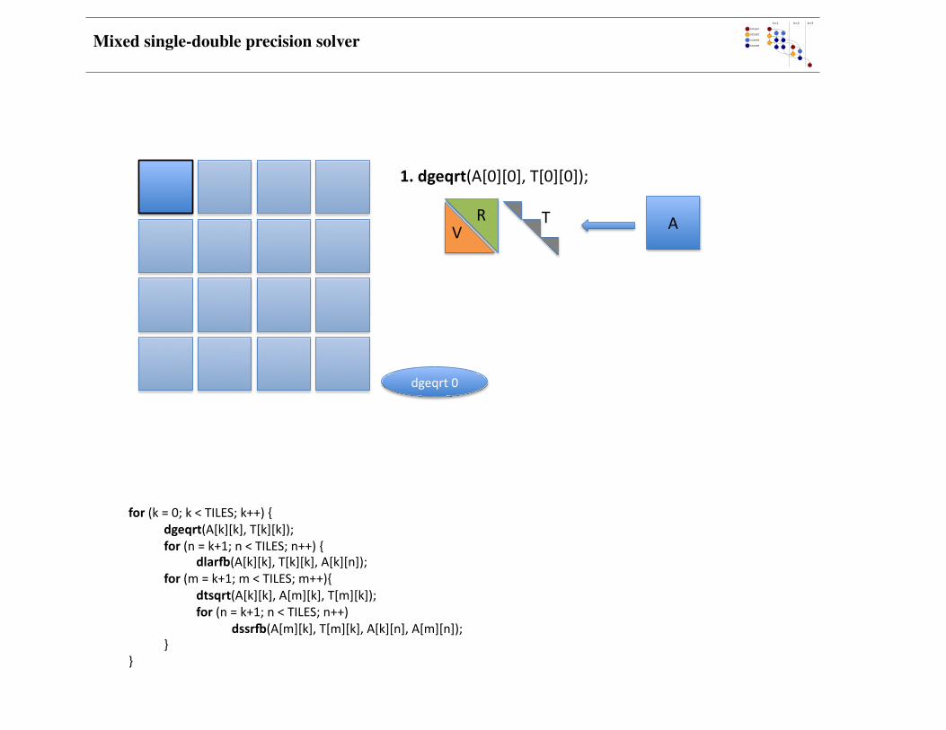
for(k=0;k<TILES;k++){dgeqrt(A[k][k],T[k][k]);for(n=k+1;n<TILES;n++){ dlar+(A[k][k],T[k][k],A[k][n]);for(m=k+1;m<TILES;m++){ dtsqrt(A[k][k],A[m][k],T[m][k]); for(n=k+1;n<TILES;n++) dssr+(A[m][k],T[m][k],A[k][n],A[m][n]);}
}
Mixed single-double precision solver
for(k=0;k<TILES;k++){dgeqrt(A[k][k],T[k][k]);for(n=k+1;n<TILES;n++){ dlar+(A[k][k],T[k][k],A[k][n]);for(m=k+1;m<TILES;m++){ dtsqrt(A[k][k],A[m][k],T[m][k]); for(n=k+1;n<TILES;n++) dssr+(A[m][k],T[m][k],A[k][n],A[m][n]);}
}
1.dgeqrt(A[0][0],T[0][0]);
VR AT
dgeqrt0

Mixed single-double precision solver
for(k=0;k<TILES;k++){dgeqrt(A[k][k],T[k][k]);for(n=k+1;n<TILES;n++){ dlar+(A[k][k],T[k][k],A[k][n]);for(m=k+1;m<TILES;m++){ dtsqrt(A[k][k],A[m][k],T[m][k]); for(n=k+1;n<TILES;n++) dssr+(A[m][k],T[m][k],A[k][n],A[m][n]);}
}
1.dgeqrt(A[0][0],T[0][0]);2.dlar+(A[0][0],T[0][0],A[0][1]);
V A
dgeqrt0
TR
dlarB0,1

Mixed single-double precision solver
for(k=0;k<TILES;k++){dgeqrt(A[k][k],T[k][k]);for(n=k+1;n<TILES;n++){ dlar+(A[k][k],T[k][k],A[k][n]);for(m=k+1;m<TILES;m++){ dtsqrt(A[k][k],A[m][k],T[m][k]); for(n=k+1;n<TILES;n++) dssr+(A[m][k],T[m][k],A[k][n],A[m][n]);}
}
1.dgeqrt(A[0][0],T[0][0]);2.dlar+(A[0][0],T[0][0],A[0][1]);3.dlar+(A[0][0],T[0][0],A[0][2]);4.dlar+(A[0][0],T[0][0],A[0][3]);
V A
dgeqrt0
TR
dlarB0,3dlarB0,2dlarB0,1

Mixed single-double precision solver
for(k=0;k<TILES;k++){dgeqrt(A[k][k],T[k][k]);for(n=k+1;n<TILES;n++){ dlar+(A[k][k],T[k][k],A[k][n]);for(m=k+1;m<TILES;m++){ dtsqrt(A[k][k],A[m][k],T[m][k]); for(n=k+1;n<TILES;n++) dssr+(A[m][k],T[m][k],A[k][n],A[m][n]);}
}
1.dgeqrt(A[0][0],T[0][0]);2.dlar+(A[0][0],T[0][0],A[0][1]);3.dlar+(A[0][0],T[0][0],A[0][2]);4.dlar+(A[0][0],T[0][0],A[0][3]);5.dtsqrt(A[0][0],A[1][0],T[1][0]);
dgeqrt0
dlarB0,3dlarB0,2dlarB0,1
V
R
A
TR
dtsqrt1,0

Mixed single-double precision solver
for(k=0;k<TILES;k++){dgeqrt(A[k][k],T[k][k]);for(n=k+1;n<TILES;n++){ dlar+(A[k][k],T[k][k],A[k][n]);for(m=k+1;m<TILES;m++){ dtsqrt(A[k][k],A[m][k],T[m][k]); for(n=k+1;n<TILES;n++) dssr+(A[m][k],T[m][k],A[k][n],A[m][n]);}
}
…4.dlar+(A[0][0],T[0][0],A[0][3]);5.dtsqrt(A[0][0],A[1][0],T[1][0]);6.dssr+(A[1][0],T[1][0],A[0][1],A[1][1]);
dgeqrt0
dlarB0,3dlarB0,2dlarB0,1
V
A
B
T
dtsqrt1,0
A
B
dssrB1,1

Mixed single-double precision solver
for(k=0;k<TILES;k++){dgeqrt(A[k][k],T[k][k]);for(n=k+1;n<TILES;n++){ dlar+(A[k][k],T[k][k],A[k][n]);for(m=k+1;m<TILES;m++){ dtsqrt(A[k][k],A[m][k],T[m][k]); for(n=k+1;n<TILES;n++) dssr+(A[m][k],T[m][k],A[k][n],A[m][n]);}
}
…4.dlar+(A[0][0],T[0][0],A[0][3]);5.dtsqrt(A[0][0],A[1][0],T[1][0]);6.dssr+(A[1][0],T[1][0],A[0][1],A[1][1]);7.dssr+(A[1][0],T[1][0],A[0][1],A[1][1]);8.dssr+(A[1][0],T[1][0],A[0][1],A[1][1]);
dgeqrt0
dlarB0,3dlarB0,2dlarB0,1
V
A
B
T
dtsqrt1,0
A
B
dssrB1,1 dssrB1,1 dssrB1,1

Mixed single-double precision solver
for(k=0;k<TILES;k++){dgeqrt(A[k][k],T[k][k]);for(n=k+1;n<TILES;n++){ dlar+(A[k][k],T[k][k],A[k][n]);for(m=k+1;m<TILES;m++){ dtsqrt(A[k][k],A[m][k],T[m][k]); for(n=k+1;n<TILES;n++) dssr+(A[m][k],T[m][k],A[k][n],A[m][n]);}
}
…4.dlar+(A[0][0],T[0][0],A[0][3]);5.dtsqrt(A[0][0],A[1][0],T[1][0]);6.dssr+(A[1][0],T[1][0],A[0][1],A[1][1]);7.dssr+(A[1][0],T[1][0],A[0][1],A[1][1]);8.dssr+(A[1][0],T[1][0],A[0][1],A[1][1]);
dgeqrt0
dlarB0,3dlarB0,2dlarB0,1
dtsqrt1,0
dssrB1,1 dssrB1,1 dssrB1,1

Mixed single-double precision solver

Mixed single-double precision solver
Execution of the parallel TSQR factorization on a binary tree of four processors. The gray boxes indicate wherelocal QR factorizations take place. The Q and R factors each have two subscripts: the first is the sequence numberwithin that stage, and the second is the stage number.

Mixed single-double precision solver
Execution of the sequential TSQR factorization on a flat tree with four submatrices. The gray boxes indicate wherelocal QR factorizations take place The Q and R factors each have two subscripts: the first is the sequence numberfor that stage, and the second is the stage number.
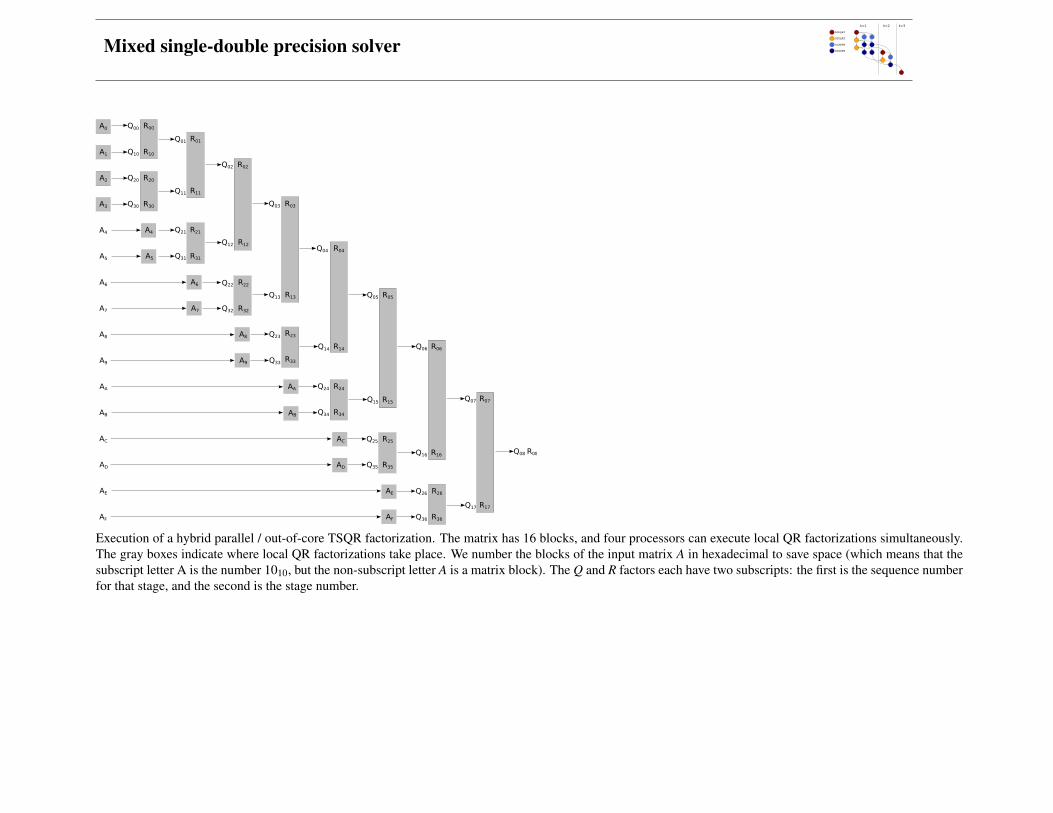
Mixed single-double precision solver
Execution of a hybrid parallel / out-of-core TSQR factorization. The matrix has 16 blocks, and four processors can execute local QR factorizations simultaneously.The gray boxes indicate where local QR factorizations take place. We number the blocks of the input matrix A in hexadecimal to save space (which means that thesubscript letter A is the number 1010, but the non-subscript letter A is a matrix block). The Q and R factors each have two subscripts: the first is the sequence numberfor that stage, and the second is the stage number.

Mixed single-double precision solver
A is m–by–n with m = pb and n = qb.We are only interested in the first step of the Householder QR factorization.
@@@@
←−
6
?
m = pb
-� n = qb

Mixed single-double precision solver
1 Classic unblocked Householder factorization: DGEQF21. DGEQR2: Panel factorization.
@@@@
←− 2mb2− 23 b3 = 2(p− 1
3 )b3
2. DLARF: Apply the V vector one-by-one to the remaining matrix. Thismakes b small step
←− (I− )
. . .
←− (I− )
∑pb`=(p−1)b+1 4(q−1)b`
= 4(q−1)b∑bi=1 (p−1)b+ i
= 4(q−1)b((p−1)b2 + 12 b2)
= (4p−2)(q−1)b3
total (4pq−2p−2q+ 43 )b3
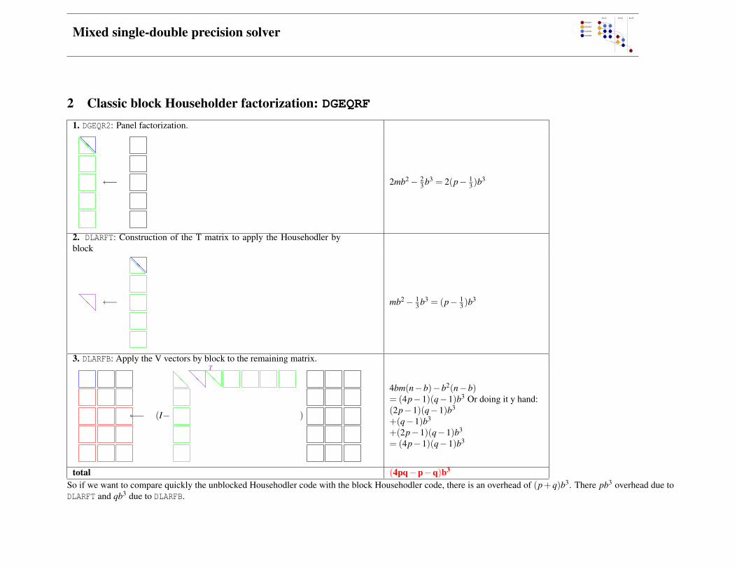
Mixed single-double precision solver
2 Classic block Householder factorization: DGEQRF1. DGEQR2: Panel factorization.
@@@@
←− 2mb2− 23 b3 = 2(p− 1
3 )b3
2. DLARFT: Construction of the T matrix to apply the Househodler byblock
@@←−
@@@@
mb2− 13 b3 = (p− 1
3 )b3
3. DLARFB: Apply the V vectors by block to the remaining matrix.
←− (I−
@@ @
@
T@@
)
4bm(n−b)−b2(n−b)= (4p−1)(q−1)b3 Or doing it y hand:(2p−1)(q−1)b3
+(q−1)b3
+(2p−1)(q−1)b3
= (4p−1)(q−1)b3
total (4pq−p−q)b3
So if we want to compare quickly the unblocked Househodler code with the block Househodler code, there is an overhead of (p+q)b3. There pb3 overhead due toDLARFT and qb3 due to DLARFB.

Mixed single-double precision solver
3 SUQRAStep 1.1.a. First QR factorization.
@@@@←− 4
3 b3
1.b DLARFT: Construction of the T matrix to apply the Househodler byblock
@@←−
@@@@
23 b3
1.c. DLARFB: Apply the V vectors by block to the remaining matrix.
←− (I−@@ @
@
T@@
) 3(q−1)b3
Step 2. (repeat this step (p−1) times.2.a. TSQR factorization (TS=triangle-square)
@@ ←−
@@ 2b3
2.b TS-LARFT: Construction of the T matrix to apply the Househodler byblock
@@←−
@@ 4
3 b3
2.c. TS-LARFB: Apply the V vectors by block to the remaining matrix.
←− (I−@@@@
T@@ ) 5(q−1)b3
total (5pq− 53 p−2q+ 2
3 )b3
This algorithm is going to perform 20% more FLOPS.⇒ Need for inner blocking.

Mixed single-double precision solver
4 SUQRA without blockingStep 1.1.a. First QR factorization.
@@@@←− 4
3 b3
1.c. DLARFB: Apply the V vectors by block to the remaining matrix.
←− Apply@@ to 2(q−1)b3
Step 2. (repeat this step (p−1) times.2.a. TSQR factorization (TS=triangle-square)
@@ ←−
@@ 2b3
2.c. TS-LARFB: Apply the V vectors by block to the remaining matrix.
←− Apply@@ to 4(q−1)b3
total (4pq−2p−2q+ 43 )b3
Exactly the same number of FLOPs as for the unblocked QR factorization

Mixed single-double precision solver
5 comparisonunblocked QR unblocked SUQRA blocked QR blockedSUQRA
panel (2p− 23 )b3 (2p− 2
3 )b3 (2p− 23 )b3 (2p− 2
3 )b3
T (p− 13 )b3 ( 4
3 p− 23 )b3
update (4pq−2q−4p+2)b3 (4pq−2q−4p+2)b3 (4pq−q−4p+1)b3 (5pq−2q−5p+2)b3
total (4pq−2q−2p+ 43 )b3 (4pq−2q−2p+ 4
3 )b3 (4pq−q− p)b3 (5pq−2q− 53 p+ 2
3 )b3
We can integrate those values to know the FLOPS count of the algorithm, we replace q by i when i varies from q to 1 and we replace p with p−q + i. We assumethat p > q, i.e. the matrix is taller than longer.This gives for the unblocked QR algorithm:
q
∑i=1
(4(p−q+ i)i−2i−2(p−q+ i)+43)b3
=q
∑i=1
(4p−4q−4)i+4i2−2p+2q+43)b3
= (4p−4q−4)q2
2+4
q3
3−2pq+2q2 +
43
q)b3
= (2pq2−2q3−2q2 +43
q3−2pq+2q2 +43
q)b3
= (2pq2− 23
q3−2pq+43
q)b3
= 2mn2− 23
n3−2mnb+43
nb2
The order is OK we find: 2mn2− 23 n3 as expected.
This gives for the block SUQRA:
q
∑i=1
(5(p−q+ i)i−2i− 53(p−q+ i)+
23)b3
∼q
∑i=1
(5pi−5qi+5i2)b3
∼ (52
pq2− 52
q3 +53
q3)b3
∼ 52
mn2− 56
n3
(1)
which means 20% overhead.

Mixed single-double precision solver
6 Remark on the panel factorizationClassical method
@@@@ ←− 2(2b)b2− 2
3 b3 103 b3
PUQRAPUQRA-step1
@@@@←−
@@@@←−
43 b3 + 4
3 b3
PUQRA-step2
@@
@@
←−@@
@@
23 b3 10
3 b3
SUQRASUQRA-step1
@@@@←− 4
3 b3
SUQRA-step2
@@ ←−
@@ 2b3 10
3 b3

Mixed single-double precision solver
DSSRFBDTSQRT
A
U T
V
B
C
Alfredo Buttari, Julien Langou, Jakub Kurzak, and Jack Dongarra. LAWN 191 – A Class of Parallel Tiled Linear Algebra Algorithms for MulticoreArchitectures, September 2007.

Mixed single-double precision solver

Mixed single-double precision solver
An interesting middleware: SMPSs
void dgeqrt(double *RV1, double *T);void dtsqrt(double *R, double *V2, double *T);void dlarfb(double *V1, double *T, double *C1);void dssrfb(double *V2, double *T, double *C1, double *C2);
cilk void qr_panel(int k){ int m;
dgeqrt(A[k][k], T[k][k]);
for (m = k+1; m < TILES; m++) dtsqrt(A[k][k], A[m][k], T[m][k]);}
cilk void qr_update(int n, int k){ int m;
dlarfb(A[k][k], T[k][k], A[k][n]);
for (m = k+1; m < TILES; m++) dssrfb(A[m][k], T[m][k], A[k][n], A[m][n]);
if (n == k+1) spawn qr_panel(k+1);}
spawn qr_panel(0);sync;
for (k = 0; k < TILES; k++) { for (n = k+1; n < TILES; n++) spawn qr_update(n, k); sync;}
Figure 14: Cilk implementation of the tile QR fac-torization with 1D work assignment and lookahead.
5.2 SMPSs Implementation
Figure 15 shows implementation using SMPSs, whichfollows closely the one for Cholesky. The func-tions implementing parallel tasks are designated with#pragma ccs task annotations defining directionalityof the parameters (input, output, inout). The par-allel section of the code is designated with #pragmaccs start and #pragma ccs finish annotations. Insidethe parallel section the algorithm is implemented us-ing the canonical representation of four loops withthree levels of nesting, which closely matches thepseudocode definition of Figure 11.
The SMPSs runtime system schedules tasks basedon dependencies and attempts to maximize datareuse by following the parent-child links in the task
#pragma css task \ inout(RV1[NB][NB]) output(T[NB][NB])void dgeqrt(double *RV1, double *T);
#pragma css task \ inout(R[NB][NB], V2[NB][NB]) output(T[NB][NB])void dtsqrt(double *R, double *V2, double *T);
#pragma css task \ input(V1[NB][NB], T[NB][NB]) inout(C1[NB][NB])void dlarfb(double *V1, double *T, double *C1);
#pragma css task \ input(V2[NB][NB], T[NB][NB]) inout(C1[NB][NB], C2[NB][NB])void dssrfb(double *V2, double *T, double *C1, double *C2);
#pragma css startfor (k = 0; k < TILES; k++) {
dgeqrt(A[k][k], T[k][k]);
for (m = k+1; m < TILES; m++) dtsqrt(A[k][k], A[m][k], T[m][k]);
for (n = k+1; n < TILES; n++) { dlarfb(A[k][k], T[k][k], A[k][n]); for (m = k+1; m < TILES; m++) dssrfb(A[m][k], T[m][k], A[k][n], A[m][n]); }}#pragma css finish
Figure 15: SMPSs implementation of the tile QR fac-torization.
graph when possible.There is a caveat here, however. V1 is an input
parameter of task dlarfb(). It also is an inout param-eter of task dtsqrt(). However, dlarfb() only readsthe lower triangular portion of the tile, while dtsqrt()only updates the upper triangular portion of the tile.Since in both cases the tile is passed to the functionsby the pointer to the upper left corner of the tile,SMPSs sees a false dependency. As a result, the ex-ecution of the dlarfb() tasks in a given step will bestalled until all the dtsqrt() tasks complete, despitethe fact that both types of tasks can be scheduled inparallel as soon as the dgeqrt() task completes. Fig-ure 16 shows conceptually the change that needs tobe done.
Currently SMPSs is not capable of recognizing ac-cesses to triangular matrices. There are however mul-tiple ways to enforce the correct behavior. The sim-
12
Figure 23 shows performance for the QR factor-ization. The situation is a little different here. Per-formance of Cilk implementations is still the poor-est and the performance of the static pipeline isstill superior. However, performance of the initialSMPSs implementation is only marginally better thatCilk 1D, while performance of the improved SMPSs*implementation is only marginally worse that staticpipeline. The same conclusions apply to the tile LUfactorization (Figure 24).
0 1000 2000 3000 4000 5000 6000 7000 80000
10
20
30
40
50
60
70
80
90
100
110Tile QR Factorization Performance
Matrix Size
Gflo
p/s
Static PipelineSMPSs*SMPSsCilk 1DCilk 2D
Figure 23: Performance of the tile QR factorization indouble precision on a 2.4 GHz quad-socket quad-core(16 cores total) Intel Tigerton system. Tile size nb =144, inner block size IB = 48.
Relatively better performance of SMPSs for theQR and LU factorizations versus the Cholesky fac-torization can be explained by the fact that the LUfactorization is two times more expensive and the QRfactorization is four times more expensive, in terms offloating point operations. This diminishes the impactof various overheads for smaller size problems.
0 1000 2000 3000 4000 5000 6000 7000 80000
10
20
30
40
50
60
70
80
90
100Tile LU Factorization Performance
Matrix Size
Gflo
p/s
Static PipelineSMPSs*SMPSsCilk 1DCilk 2D
Figure 24: Performance of the tile LU factorization indouble precision on a 2.4 GHz quad-socket quad-core(16 cores total) Intel Tigerton system. Tile size nb =200, inner block size IB = 40.
8 Conclusions
In this work, suitability of emerging multicore pro-gramming frameworks was analyzed for implement-ing modern formulations of classic dense linear alge-bra algorithms, the tile Cholesky, the tile QR andthe tile LU factorizations. These workloads are rep-resented by large task graphs with compute-intensivetasks interconnected with a very dense and complexnet of dependencies.
For the workloads under investigation, the con-ducted experiments show clear advantage of themodel, where automatic parallelization is based onconstruction of arbitrary DAGs. SMPSs providesmuch higher level of automation than Cilk and simi-lar frameworks, requiring only minimal programmer’sintervention and basically leaving the programmeroblivious to any aspects of parallelization. At thesame time it delivers superior performance throughmore flexible scheduling of operations.
SMPSs still looses to hand-written code for veryregular compute-intensive workloads investigated
17
From:
• Jakub Kurzak, Hatem Ltaief, Jack Dongarra, and Rosa M.Badia. Scheduling Linear Algebra Operations on Multi-core Processors. LAWN 213.
See also:
• Rosa M. Badia, Jose R. Herrero, Jesus Labarta, Josep M.Perez, Enrique S. Quintana-Ortı, and Gregorio Quintana-Ortı. Parallelizing dense and banded linear algebra li-braries using SMPSs. UPC-DAC-RR-2008-64.
• Hatem Ltaief, Jakub Kurzak, and Jack Dongarra. Schedul-ing Two-sided Transformations using Algorithms-by-Tileson Multicore Architectures. LAWN 214.

Mixed single-double precision solver
Alfredo Buttari, Julien Langou, Jakub Kurzak, and Jack Dongarra. LAWN 191 – A Class of Parallel Tiled Linear Algebra Algorithms for MulticoreArchitectures, September 2007.

Mixed single-double precision solver
2000 4000 6000 8000 10000 120000
10
20
30
40
50
60
70
80
Cholesky −− 2−way Quad Clovertown
problem size
Gflo
p/s
DGEMM peak
LAPACKMKL−9.1Tiled+asynch.
Alfredo Buttari, Julien Langou, Jakub Kurzak, and Jack Dongarra. LAWN 191 – A Class of Parallel Tiled Linear Algebra Algorithms for MulticoreArchitectures, September 2007.

Mixed single-double precision solver
2000 4000 6000 8000 10000 120000
10
20
30
40
50
60
70
80
QR −− 2−way Quad Clovertown
problem size
Gflo
p/s
DGEMM peak
LAPACKMKL−9.1Tiled+asynch.
Alfredo Buttari, Julien Langou, Jakub Kurzak, and Jack Dongarra. LAWN 191 – A Class of Parallel Tiled Linear Algebra Algorithms for MulticoreArchitectures, September 2007.

Mixed single-double precision solver
0 500 1000 1500 2000 2500 3000 3500 40000
20
40
60
80
100
120
140
160
180
200Tile QR Factorization −− 3.2 GHz CELL Processor
Matrix Size
Gflo
p/s
SSSRFB PeakTile QR
Figure 5: Performance of the tile QR factorization in single precision on a 3.2GHz CELL processor with eight SPEs. Square matrices were used. The solidhorizontal line marks performance of the SSSRFB kernel times the numberof SPEs (22.16! 8 = 177 [Gflop/s]).
28
Performance of the tile QR factorization in single precision on a 3.2 GHz CELL processor with eight SPEs.Square matrices were used. Solid horizontal line marks performance of the SSSRFB kernel times the number ofSPEs (22.16×8 = 177 [Gflop/s]).
“The presented implementation of tile QR factorization on the CELL processor allows for factorization of a 4000–by–4000 dense matrix in single precision in exactly half of a second. To the author’s knowledge, at present, it is thefastest reported time of solving such problem by any semiconductor device implemented on a single semiconductordie.”
Jakub Kurzak and Jack Dongarra, LAWN 201 – QR Factorization for the CELL Processor, May 2008.

Mixed single-double precision solver
QandR:Strongscalability
0
100
200
300
400
500
600
700
800
32 64 128 256
ReduceHH(QR3)
ReduceHH(QRF)
ScaLAPACKQRF
ScaLAPACKQR2
Inthisexperiment,wefixtheproblem:m=1,000,000andn=50.Thenweincreasethenumberofprocessors.BlueGeneL
frost.ncar.edu
#ofprocessors
MFLOPs/sec/proc

Mixed single-double precision solver

Mixed single-double precision solver

Mixed single-double precision solver
Strategy:
1. obtain some lower bounds for the cost (latency, bandwidth, # of operations) of LU, QR and Cholesky insequential and parallel distributed
2. compute the costs of our algorithms and compare with the lower bound.
Lower bounds:
1. For LU, observe that: I 0 −BA I 00 0 I
=
IA I0 0 I
I 0 −BI A ·B
I
therefore lower bound for matrix-matrix multiply (latency, bandwidth and operations) also holds for LU.
2. For Cholesky, observe that: I AT −BA I +AAT 0−BT 0 D
=
IA I−BT (A ·B)T X
I AT −BI A ·B
XT
however this gets nasty due to the AAT term in the initial matrix A. See Grey Ballard, James Demmel,Olga Holtz, and Oded Schwartz. Communication-optimal Parallel and Sequential Cholesky decomposition.UCB/EECS-2009-29, February 13th, 2009.
3. For QR, we needed to redo the proof of optimality of matrix-matrix multiply. See James W. Demmel, LauraGrigori, Mark F. Hoemmen, and Julien Langou. Communication-avoiding parallel and sequential QR factor-izations. arXiv:0902.2537, May 30th, 2008.

Mixed single-double precision solver
New Algorithm ScaLAPACK AlgorithmPar. CAQR PDGEQRF Lower bound
# flops(4
3
) · (n3/P)
X(4
3
) · (n3/P)
X O(n3/P
)# words
(34 · logP
) · (n2/√
P)
X(3
4 · logP) · (n2/
√P)
X O(n2/√
P)
# messages(3
8 · log3 P) · (√P
)X
(54 · log2 P
) · (n) × O(√
P)
New Algorithm X ScaLAPACK ×
Performance models of parallel CAQR and ScaLAPACK’s parallel QR factorization PDGEQRF on a square n×nmatrix with P processors, along with lower bounds on the number of flops, words, and messages. The matrixis stored in a 2-D Pr×Pc block cyclic layout with square b× b blocks. We choose b, Pr, and Pc optimally andindependently for each algorithm. Everything (messages, words, and flops) is counted along the critical path.

Mixed single-double precision solver
Seq. CAQR Householder QR Lower bound# flops 4
3n3 43n3 O(n3)
# words 3 n3√W
13
n4
W O( n3√W
)
# messages 12 n3
W 3/212
n3
W O( n3
W 3/2)
Performance models of sequential CAQR and blocked sequential HouseholderQR on a square n×n matrix with fast memory size W , along with lower boundson the number of flops, words, and messages.

Mixed single-double precision solver
Opportunities for further research:
how to tile the matrix? square blocks, nonsquare blocks?
kernel tuning: introduction of a lots of new kernels (e.g. QR fact. of a triangle on top of a square). For eachkernel:
1. how to optimize the blocking parameter (nb)?
2. which algorithmic variants to choose (left looking, recursive, ...) ?
3. the inner blocking parameter (ib).
Question 2 and 3 are standard autotuning problems. Choosing ib and the algorithmic vairant is done in termof nb. Question 1 is more subtle. Choosing nb is done at the matrix level (n) since it influences the granularityof the algorithm.
reduction algorithm: Which reduction tree to use? Binary tree? Flat tree? Hybrid tree? Each of these choicesrepresent an algorithm change. No framework to accomodate this yet.
scheduling: How to schedule all these tasks?
1. static scheduling or dynamic scheduling?
2. and in parallel distributed ...