julia andrade - solubility calculations for hydraulic gas ... · pdf filej. andrade solubility...

MIRARCO MINING INNOVATION RESEARCH REPORT

Solubility Calculations for Hydraulic Gas

Compressors

JULIA ANDRADE

21 August 2013

J. Andrade Solubility Calculations for Hydraulic Gas Compressors 21 August 2013

2/30

Table of Contents

1 Introduction ................................................................................................................................ 5

2 Vapor-Liquid Equilibrium (VLE) Theory .................................................................................. 7

2.1 Henry’s Law Applied for Solubility Calculations ............................................................. 8

2.1.1 Henry’s Law .............................................................................................................. 8

2.1.2 Henry’s Constant ....................................................................................................... 9

2.1.3 Limitations of Henry’s Law .................................................................................... 10

2.2 Cubic Equations of State applied for solubility calculations ........................................... 10

3 Approximation of the vapour-liquid equilibrium of air in water .............................................. 14

3.1 Applying Henry’s Law - Estimating Henry’s Constant from van’t Hoff Expression ...... 14

3.2 Applying Henry’s Law - Estimating Henry’s Constant from Analytical Expressions .... 15

3.3 Comparison with Experimental Data from the Literature ............................................... 16

4 Approximation of the vapour-liquid equilibrium of combustion gases in water ...................... 19

4.1 Combustion gases from different fuels ............................................................................ 19

4.1.1 Estimation of the Solubility of Combustion Gases using Henry’s Law .................. 20

5 Approximation of the vapour-liquid equilibrium of carbon dioxide in water ........................... 22

5.1 Estimating the solubility of CO2 in water using Henry’s Law......................................... 22

5.2 Experimental Data of the System CO2 + Water ............................................................... 23

5.3 Estimating the solubility of CO2 in water using the VR Therm ...................................... 24

5.4 Limitations of Henry’s Law in predicting the solubility of the system CO2 + Water...... 25

5.5 Estimating the solubility of CO2 in water using the model of Diamond (2003) .............. 26

6 Conclusions ............................................................................................................................... 28

7 References ................................................................................................................................. 29


3/30

List of Figures

Figure 1 – Schematic Diagram of a Hydraulic Air Compressor ......................................................... 6

Figure 2 - Mass of N2, O2 and Ar in the gas phase as the absolute pressure of the system increases 15

Figure 3 - Solubility of air in water at pressure ranging from 0 to nearly 1,200 meters of water:

Results from the Application of Henry's Law and Kolev's Correlations and Experimental Data from

[15] and [16] ...................................................................................................................................... 18

Figure 4 - Pressures at which all CO2 is dissolved in water for the fuel methane, diesel, anthracite

and HFSO .......................................................................................................................................... 21

Figure 5 - Solubility of CO2 in water at 50°C obtained applying Henry's Law ................................ 22

Figure 6 - Solubility of CO2 in water at pressure ranging from 0 to nearly 1,500 meters of water:

Results from the Application of Henry's Law and S-P-E [20] and P-CO2 [16] Experimental Data . 24

Figure 7 - Solubility of CO2 in water predicted from SKR EoS and PR EoS, using the VRTherm,

compared with the S-P-E Experimental Data.................................................................................... 25

Figure 8 - CO2 solubility in water at 50°C using the model from [22] referred as D-A Data in

comparison with S-P-E and P-CO2 experimental data ...................................................................... 27

List of Tables

Table 1: Values of molar fraction, Henry's Law Constants and Temperature Dependence .............. 10

Table 2: B-R-T Data of Air Solubility in Water Expressed as a Mass Fraction (gram of air per gram

of water) ............................................................................................................................................ 17

Table 3: Henry's Law Constants for the Solubility of Air in Water as atm....................................... 17

Table 4: Composition of the flue gases from the complete combustion of fuels with oxygen

contained in air in molar fraction ...................................................................................................... 20

Table 5 - Solubility of CO2 in water: Experimental Data at 50°C and from nearly 10 to 7,233 meters

of water.............................................................................................................................................. 23


4/30

Nomenclature

Symbol Name

P Absolute Pressure

� Acentric factor

�� Activity coefficient of component � �� Binary Interaction Parameter

� Compressibility Factor

P Critical pressure

T Critical temperature

�� Fugacity of component � in a multicomponent mixture

�� Fugacity of pure species � in phase �

�� Fugacity of species � in phase � in a multicomponent mixture

�� K-value of equilibrium

�� Henry’s Constant

�� Mole fraction of component � in the liquid phase

�� Mole fraction of component � in the gas phase

� Molar gas constant

�� Molecular weight

�� Partial pressure of a gas � ∆�� Solute enthalpy of solution

Specific volume

T Temperature


5/30

1 Introduction

There are many studies of gas solubility in water, both experimental and theoretical, especially at

the low-pressure region, where partial pressures do not exceed a few atmospheres. If working in this

low-pressure region there are advantages, such as; the majority of the data are reliable and of high

precision, the thermodynamic relations are estimated by generally-accepted and well-defined

correlations, and the results are barely influenced by inaccuracies from semi-empirical data. High-

pressure equilibrium data encounters thermodynamic difficulties for analysis, because of the

complexity of the mathematical formalism, the absence of fundamental data, and the dependence on

empirical correlations for their estimation [1].

The reliable estimation of high-pressure vapour-liquid equilibrium is important for a variety of

applications, especially in the chemical engineering field. For instance, due to concerns with global

warming, equilibrium data is essential for the study of sequestration of carbon dioxide (CO2) when

capturing and injecting it into deep geological formations [2]. A more specific application is in the

analysis of air loss in hydraulic air compressors (HACs). These involve the pressurisation of air by

water hence determining the solubility of air in water during the compression process is vital to

determine the loss of gaseous species due to their solution and for the correct operation of the other

elements of the equipment, such as air water separation [3].

An hydraulic air compressor can produce compressed air by the means illustrated in Figure 1. The

hydraulic energy source is a head of water, and its downward moving flow entrains air. The

separation of the air from the water at depth produces compressed air.


6/30

Figure 1 – Schematic Diagram of a Hydraulic Air Compressor

The applications for HACs range from wave energy recovery to the production of compressed air

for compressed air energy storage. The performance of the HAC can be adversely affected by the

absorption of air by water during the compression process, representing a loss of product for the

equipment. Consequently, the accurate estimation of the maximum impact of air solubility by

applying vapor-liquid equilibrium calculations is essential for the modeling of the two-phase flow

in HACs.

The range of applications for hydraulic compressors has recently been conceptually extended to the

sequestration of combustion gases, such as carbon dioxide, a so-called greenhouse that is important

in global warming. In this case, the more gas that is absorbed by water, the better the sequestration

performance by hydraulic gas compression. Therefore, again, accurate calculations for gas

solubility in water are essential for the proper evaluation of HAC equipment performance in this

context.

Taking into account the importance of predicting the amount of gases absorbed by water during

hydraulic gas compression, this work focus on the estimation of solubility of gaseous species in air

and combustion gases at elevated pressure. Firstly, a discussion of the thermodynamic fundamentals

of vapour-liquid equilibrium is presented, followed by solubility calculations and their comparison

with experimental data. The results provided by this study aim to be used to update the

hydrodynamic calculations of hydraulic gas compressors (as a generalisation of hydraulic air

compressors).


7/30

2 Vapor-Liquid Equilibrium (VLE) Theory

According to [5], thermodynamically, the equilibrium state is defined as:

“The equilibrium state of a closed system at a given P and T is the one for which the Gibbs free

energy of the system is at a minimum with respect to all possible changes.”

As a consequence of this definition and as exposed in details by Smith and Van Ness [10], there is

equilibrium between phases at the same P and T when the fugacity of each species (��) is the same

in all phases. Systems involving a single liquid phase in equilibrium with its vapor phase are in

vapor-liquid equilibrium (VLE) and the criterion for equilibrium is written as:

��! = �� (1)

Fugacity is a thermodynamic property that has dimensions of pressure and is given by:

�� = ��#$%��#$&�� '()*+,+(-./012 (2)

where the exponential component is known as the Poynting factor.

For the case of multi-component vapor-liquid equilibrium, Equation (1) becomes:

��!� = ��4 (�=1, 2, ..., N) (3)

where N is the number of components in the mixture.

The dimensionless ratio �/% is a mixture property called the fugacity coefficient and given the

symbol �. The fugacity coefficient of species � in solution is given the symbol �� and defined as:

�� ≡ 7847889� (4)

where ��:� represents the fugacity of a species in an ideal-gas mixture and is equal to the partial

pressure of the species:

��:� = ��% (5)

The activity coefficient of species � in solution is defined as follows and depends upon the

chemicals involved, particularly whether they are polar or not (i.e. have a dipole moment) [5].

�� ≡ 784;(7( (6)


8/30

For species � in the vapor mixture, the combination of Equations (4) and (5) becomes:

��!� = �� % (7)

and for species � in the liquid solution, Equation (6) is written as:

��4 = ��. (8)

As stated in Equation (3), at equilibrium the two above equations must be equal, therefore:,

�� % = �� (9)

2.1 Henry’s Law Applied for Solubility Calculations

2.1.1 Henry’s Law

William Henry in 1803 pioneered work describing the solubility of gases in water. Henry’s Law

states that the fugacity of a component in the gas phase can be linearly related to its liquid

concentration, when the mixture is sufficiently diluted, and is expressed as: [6]

��! = �� → 0� (10)

Where �� is a proportionality constant called Henry’s Constant.

For relatively low pressures (up to 2 MPa, typically) and dilute solutions (�� < 0.03, typically),

ideal gas phase behaviour can be assumed. Substituting ��! into Eq. (5) and solving for ��, Henry’s

law becomes: [6]

�� = A(B( �� → 0, DEF%� (11)

where �� is the partial pressure of the gas.

In Eq. (11) gas solubility is expressed in terms of mole fractions; nevertheless, the solubility can be

expressed in terms of mass fractions, volume fractions, molarity (moles per litre of solution), and

molality (moles per kilogram of solvent). Consequently, Henry’s law can be expressed in a variety

of ways depending on the dimensional units employed. [7] For instance, if it is desirable to state the

solubility inG:9.-:-H) I, Eq. (11) can be modified to:

J� = ��. ��. K(L-H) (12)


9/30

where J� is the solubility of the component � in G :(:-H)I, �� is its partial pressure in MNOPQ, �� is its

molecular weight inG :(R��(I, and S�� is the density of the solution G:-H)T-H)I. Taking into account the

units adopted, the dimensional unit of �� must be G�R��(/T-H)�#$R I.

2.1.2 Henry’s Constant

For pressures up to 5 MPa, the effects of pressure on Henry’s Constant are quite small and it can be

considered that �� is solely a function of temperature. Qualitatively, the significant non-linear

temperature dependence generally increases with temperature at low temperatures, reaches a

maximum, and then decreases at high temperatures. The temperature at which the maximum �� occurs depends on the specific solute-solvent pair. As a guideline, the maximum tends to increase

with increasing solute critical temperature for a given solvent and with increasing solvent critical

temperature for a given solute. Inaccuracies can result, if the temperature dependence is ignored.

The Henry’s Constant can be extrapolated from a single data point at a certain temperature using the

van’t Hoff expression [8]:

B(�2U�B(�2V� ≈ &�� GX∆B-H)

1 Y X Z2U − Z

2VYI (13)

where ∆�� is the solute enthalpy of solution and � is the molar gas constant. The temperature

dependence is:

∆B-H)1 = − \ ]^B(

\�Z 2⁄ � (14)

The van’t Hoff approach assumes that ∆�� remains constant with temperature; hence, the

expression is usually a fair approximation of Henry’s Constant for modest temperature differences

when independent values of ∆�� exist at the desired temperature, either from calorimetric data, or

from a reliable estimation techniques[8]. Sander [9] presents a compilation of Henry’s Constants at

�̀ =298.15 K, as well as the temperature dependence defined in Eq. (14). In this work, the most

frequent values of those constants were adopted for the components of interest and are shown in

Table 1.


10/30

Table 1: Values of molar fraction, Henry's Law Constants and Temperature Dependence

Air component a N2 O2 Ar CO2 SO2

��̀ � XPED� �b. NOP�c Y 0.00061 0.0013 0.0014 0.034 1.2

− d ln��d�1 �⁄ �� 1,300 1,500 1,100 2,400 3,200

2.1.3 Limitations of Henry’s Law

The Henry’s Law constants can be satisfactorily used to express solubility, but it must be

remembered from thermodynamics that it is a limiting law applicable only for dilute solutions. [7]

The larger the deviations from ideal behaviour of the system, the narrower the range of

concentrations suitable for the application of Henry’s Law. Moreover, Henry’s Law is restricted to

describe the equilibrium of a single species that does not react chemically with the solvent. Hence,

Henry’s Law cannot predict the actual equilibrium when the aqueous form of a substance is

partitioned within the aqueous phase; for instance, carbon dioxide (CO2) in water quickly forms

hydrated carbon dioxide and then carbonic acid (H2CO3). [8]

2.2 Cubic Equations of State applied for solubility calculations

In the case of mixtures that largely deviate from the ideal behaviour the equilibrium relation of Eq.

(3) can be represented by:

��%�h�! = ��%�h�� or simply:

��h�! = ��h�� = 1, 2, . . . , N� (15)

Eq. (15) may be written as

�� = �� = 1, 2, . . . , N� (16)

where �� is the K-value given by:

�� = k ()k (l (17)

From [10], the general equation for calculating the fugacity coefficients �h�� and �h�! is:

ln�� = � − 1 − ln� − m nXo�pq�op( Y2,',pr − 1s \'''t (18)


11/30

where � is the compressibility factor defined as the ratio % ��⁄ and calculated from Equations of

State (EoS) that relate pressure, temperature and specific volume ( ). For ideal gases, � equals one

and the EoS becomes:

% = �� (19)

EoS are the basis of thermodynamic models and are used to represent phase equilibria, as well as

the calculation of thermal and volumetric properties [11]. Under high pressures, the P-V-T

behaviour is not correctly represented by the ideal gas EoS. In 1873, the first generalization known

as van der Waals Equation of State was proposed: [12]

% = 12!,u − #

!v (20)

where N accounts for the interaction forces between two molecules and w accounts for the excluded

volume.

Numerous models based on van der Waals EoS were formulated since its advent. They are

conventionally called cubic equations of state, since they can be rearranged to be cubic in , as

shown in Eq. 21. [5]

x − Xw + 12+ Y z + #

+ − #u+ = 0 (21)

The cubic EoS provide great advantage over other complex EoS, such as: accuracy of the results,

computational efficiency, and ease of implementation [13]. One of the variations of the van der

Waals EOS is the Soave-Redlich-Kwong (SRK) EoS proposed in 1972, which is common in

process simulators: [12]

% = 12!,u − #

!�!{u� (22)

Where: (from [9]):

N = 0.42748X�v��v�� Yα;

w = 0.08664X12�+� Y;

�� = 22�;


12/30

� = �1 + P*1 − ��`.�0�z, and;

P = 0.480 + 1.574 − 0.176�z.

The Peng-Robinson equation of state (PR) from 1976 is another variation given as:

% = 12!,u − #

!�!{u�{u�!,u� (23)

Where:

N = 0.45724X�v��v�� Yα,

w = 0.08664X12�+� Y,

� = �1 + P*1 − ��`.�0�z, and;

P = 0.37464 + 1.54226 − 0.26992�z.

The critical temperature (T), critical pressure (P), and ‘acentric’ factor (�) are tabulated pure-fluid

physical properties [12].

The extension of an EoS from pure gas to mixtures requires the employment of empirical mixing

rules that represent the composition dependence of the parameters. Soave (1972) suggested

determining N and w from:

N = ∑ ∑ ��N��Z��Z (24)

w = ∑ ��w��Z (25)

where �� and �� are the mole fractions of component i and j, respectively, in the vapour or liquid

phase. The term w� is the b-parameter defined above for the ith component. The term N�� is

determined as:

N�� = �*N�N�0�1 − �� (26)

The parameter �� is a binary interaction parameter for each binary component pair. �� is zero by

definition if � = � and it is close to zero for two different components of approximately the same

polarity. Otherwise, the binary interaction parameter is tabulated.


13/30

For the SRK EoS, the expression for the fugacity coefficient of component � in a mixture takes the

form: [5]

ln�� =− ln�� − �� + �� − 1� u(u − �� GZ# *2�N� ∑ ��N�*1 − ��0��Z 0 − u(

u I ln X1 + �qY (27)

In comparison, the PR EoS expression for the fugacity is: [5]

ln�� =− ln�� − �� + �� − 1� u(u − �zU.�� GZ# *2�N� ∑ ��N�*1 − ��0��Z 0 − u(

u I ln Xq{*zV.�{Z0�

q,�zV.�,Z��Y (28)


14/30

3 Approximation of the vapour-liquid equilibrium of air in water

In this work, the solubility of air in water was analysed for a temperature of 298.15K and for

pressures ranging from approximately 1 to 97 atm. The air was considered a mixture of nitrogen,

oxygen, and argon in a concentration expressed in molar fraction of 0.7557, 0.2316, and 0.012691,

respectively. These values were taken from the NIST Reference Fluid Thermodynamic and

Transport Properties Database Version 9.1 (REFPROP) and the other components of air were not

included due to their relative low concentration.

3.1 Applying Henry’s Law - Estimating Henry’s Constant from van’t Hoff Expression

Firstly, the solubility of air in water was approximated using Henry’s law. Since our temperature of

interest (298.15K) is the same as the temperature of reference of the Henry’s Law constants shown

in Table 1, it was not necessary recalculate Henry’s constants for the air components. The higher

the��, the higher the solubility of the component in water; therefore argon dissolves in water faster

than nitrogen and oxygen.

Knowing the value of ��, the solubility of air in water was estimated as G:.(�:-H)I , by applying Eq. (12)

in the pressure range of interest, using intervals of 0.5 atm. In this work we considered the flow of

water as 20,000 kg/s and the flow of air as 20 kg/s. The initial mass of component i in the air was

determined by multiplying the composition of air by its flow, and as the pressure increased, the

mass of a gaseous species in air was calculated by subtracting the amount transferred to the water.

The mass of each component in water at a certain pressure was estimated by multiplying its

solubility at that pressure for the flow of water (20,000 kg/s); and the mass transferred from the air

to the liquid phase was considered to be the difference of its mass in water at each pressure. Figure

2 illustrates the mass behaviour in the gas phase for each component of air analysed and, as

predicted, argon is the first component to become entirely removed from the gas phase, due to its

higher solubility in water, and nitrogen is the last one to be completely removed.

J. Andrade Solubility Calculations for Hydraulic Gas Compressors

Figure 2 - Mass of N2, O2 and Ar in the gas phase as the absolute pressure of the system increases

3.2 Applying Henry’s Law Expressions

In his book, Multiphase Flow Dynamics, Kolev

literature on the solubility of O

expressions in order to ease their application in computational s

following recommended expressions of

��v��, %� = �NZ + Nz� + Nx�

where:

NZ:� = −133424.80726−7.78632 ∗

��v�� = 10�&��MNZ + Nz�̅ + N�NZ` + NZZ�̅ + NZz�̅z� ln �Q where:

NZ:Zz = −2.10973

Solubility Calculations for Hydraulic Gas Compressors 21 August 2013

15/30

and Ar in the gas phase as the absolute pressure of the system increases

Applying Henry’s Law - Estimating Henry’s Constant from Analytical

In his book, Multiphase Flow Dynamics, Kolev [14] collected experimental data available in the

literature on the solubility of O2, N2, H2 and CO2 in water and correlated them with analytical

expressions in order to ease their application in computational simulations. In the present work, the

following recommended expressions of �� for N2 and O2 in water are applied:

�z�10¡ + �N¢ + N�� + N¡�z�%10 + �N£ + N¤� + N

80726, 826.81456,−1.17389,−66.79008,0.4994610,¢, 0.02728,−2.03146 ∗ 10,¢, 3.28 ∗ 10,£

Nx�̅z + �N¢ + N��̅ + N¡�̅z�� + �N£ + N¤�̅ + N��̅z��Q (30)

∗ 10z, 2.32745,−1.19186 ∗ 10,z, −2.02733 ∗ 10,

21 August 2013

Estimating Henry’s Constant from Analytical

collected experimental data available in the

in water and correlated them with analytical

imulations. In the present work, the

N��z�%z10,¢

(29)

49946,

��z +

,Z,


16/30

2.45925 ∗ 10,x, −1.21107 ∗ 10,�, 9.77301 ∗ 10,�, −1.43857 ∗ 10,¡, 6.84983 ∗ 10,�, 4.79875 ∗ 10Z, −5.14296 ∗ 10,Z, 2.61610 ∗ 10,x

And

�̅ = % 10�⁄ .

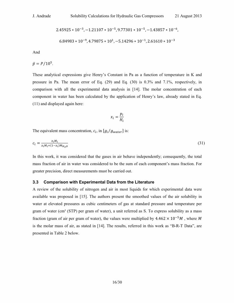
These analytical expressions give Henry’s Constant in Pa as a function of temperature in K and

pressure in Pa. The mean error of Eq. (29) and Eq. (30) is 0.3% and 7.1%, respectively, in

comparison with all the experimental data analysis in [14]. The molar concentration of each

component in water has been calculated by the application of Henry’s law, already stated in Eq.

(11) and displayed again here:

�� = ��

The equivalent mass concentration, J�, in M¥� ¥¦#$§�⁄ Q is:

J� = ;(K(;(K({�Z,;(�K¨v©

(31)

In this work, it was considered that the gases in air behave independently; consequently, the total

mass fraction of air in water was considered to be the sum of each component’s mass fraction. For

greater precision, direct measurements must be carried out.

3.3 Comparison with Experimental Data from the Literature

A review of the solubility of nitrogen and air in most liquids for which experimental data were

available was proposed in [15]. The authors present the smoothed values of the air solubility in

water at elevated pressures as cubic centimeters of gas at standard pressure and temperature per

gram of water (cm³ (STP) per gram of water), a unit referred as S. To express solubility as a mass

fraction (gram of air per gram of water), the values were multiplied by 4.462 × 10,�� , where �

is the molar mass of air, as stated in [14]. The results, referred in this work as “B-R-T Data”, are

presented in Table 2 below.


17/30

Table 2: B-R-T Data of Air Solubility in Water Expressed as a Mass Fraction (gram of air per gram of water)

T, K 1 MPa 5 MPa 10 MPa 15 MPa 20 MPa 25 MPa

273.15 0.000267 0.001505 0.002959 0.004212 0.005246 0.006086

278.15 0.000242 0.001361 0.002675 0.003812 0.004742 0.005505

283.15 0.000221 0.001243 0.002442 0.003476 0.004342 0.005026

288.15 0.000204 0.001146 0.002248 0.003205 0.003993 0.004639

293.15 0.00019 0.001066 0.002093 0.002985 0.003721 0.004303

298.15 0.000177 0.000999 0.001964 0.002791 0.003489 0.004032

303.15 0.000168 0.000942 0.001848 0.002636 0.003282 0.003812

308.15 0.000159 0.000895 0.001757 0.002507 0.003127 0.003618

313.15 0.000152 0.000858 0.001693 0.002403 0.002998 0.003463

318.15 0.000147 0.000826 0.001628 0.002313 0.002881 0.003334

323.15 0.000142 0.0008 0.001576 0.002235 0.002791 0.00323

328.15 0.000138 0.000779 0.001538 0.002184 0.002714 0.003153

333.15 0.000136 0.000764 0.001499 0.002132 0.002662 0.003088

338.15 0.000133 0.000751 0.001473 0.002106 0.002623 0.003037

343.15 0.000132 0.000742 0.00146 0.00208 0.002584 0.002998

According to Perry’s Handbook of Chemical Engineering [16], which presents tabulated values of

Henry’s Law constants over a range of temperatures (Table 3), at 25°C (298.15K) Henry’s Constant

is equal to 72,000 atm. Applying Eq. (11) in conjunction with Eq. (31) and considering the partial

pressure in the vapor phase equals to the total pressure of the system, the mass fraction of air in

water was obtained (P-Air Results) for the range of pressures analysed.

Table 3: Henry's Law Constants for the Solubility of Air in Water as atm

T, °C 0 5 10 15 20 25 30 35

10⁻⁴ ·�� 4.32 4.88 5.49 6.07 6.64 7.20 7.71 8.23

T, °C 40 45 50 60 70 80 90 100

10⁻⁴ ·�� 8.70 9.11 9.46 10.1 10.5 10.7 10.8 10.7

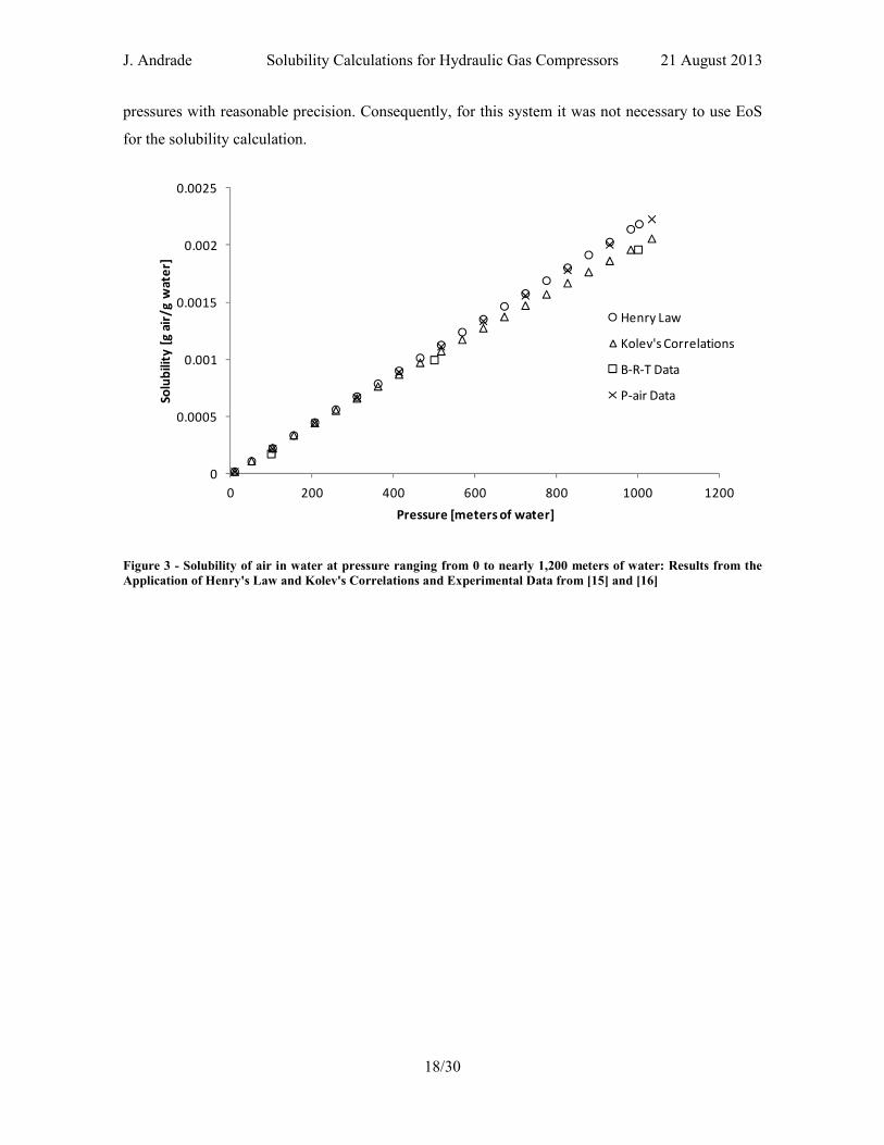
The graph in Figure 3 presents the solubility of air in water calculated via the estimation of �� using

the van’t Hoff expression, as well as, via the application of Kolev’s correlations, as described in

Sections 3.1 and 3.2, respectively. In addition, the B-R-T Results and P-air Results are also plotted.

From the graph, up to pressures equivalent to 300 meters of water, the solubility calculated in this

work matches the values from the literature (B-R-T and P-air Results) with good accuracy. At

pressures higher than 300 meters of water, the results from Henry’s Law approximate more closely

with the P-air; whereas, the use of Kolev’s Correlations lead to values closer to the B-R-T Results.

Overall, from the comparison, the results from this work closely agree with the experimental data.

Hence, it can be said that Henry’s Law is able to predict the solubility of air in water at high


18/30

pressures with reasonable precision. Consequently, for this system it was not necessary to use EoS

for the solubility calculation.

Figure 3 - Solubility of air in water at pressure ranging from 0 to nearly 1,200 meters of water: Results from the

Application of Henry's Law and Kolev's Correlations and Experimental Data from [15] and [16]

0

0.0005

0.001

0.0015

0.002

0.0025

0 200 400 600 800 1000 1200

So

lub

ilit

y [

g a

ir/

g w

ate

r]

Pressure [meters of water]

Henry Law

Kolev's Correlations

B-R-T Data

P-air Data


19/30

4 Approximation of the vapour-liquid equilibrium of combustion gases in water

4.1 Combustion gases from different fuels

Combustion is defined as a “chemical process of oxidation that occurs at a rate fast enough to

produce temperature rise and usually light, either as a glow or flame” [17]. In this work, the

complete combustion of the fuels: methane, diesel, anthracite, and high-sulphur fuel oil (HSFO)

with oxygen was studied. The solubility of the flue gases in water, especially CO2, was also

analysed. Herein, the source of the oxidizing element (oxygen) was air with a composition of

78.12% N2, 20.96% O2 and 0.92% Ar in molar percentage.

The combustion reactions for methane and diesel with air are based on the general formulas of these

compounds, «�¢ and «Zz�zx, respectively, and are explicit in the equations:

1«�¢ + 2¬z + 7.45z + 0.09®¯ → 1«¬z + 7.45z + 0.09®¯ + 2�z¬

1«Zz�zx + 17.75¬z + 66.16z + 0.78®¯ → 12«¬z + 66.16z + 0.78®¯ + 11.5�z¬

The composition of the flue gases on a dry basis is determined by the stoichiometry of these

equations, associated with the formula mass of the components, and is shown in Table 4.

In the case of anthracite and HSFO, there are no general compound formulae available in the

literature; however, in [18] the authors propose a methodology to calculate the carbon to CO2 mass

conversion factor for HFSO and the result was 3.021 - read as: 3.021 mass units of CO2 emitted per

each mass unit of HFSO combusted. The HFSO analysis from [18] indicated 2.7 wt% sulphur (S)

content; hence, we calculated the Sulphur to SO2 mass conversion factor for HFSO as 0.054 using

the same methodology. In [19], the authors presented an ultimate analysis of a raw anthracite coal

from China and the mass percentage of C is 92.27%. In this work, we considered that all the other

components are inert, including sulphur, since its content of 0.79% is negligible. Based on the

methodology of [18], the carbon to CO2 mass conversion factor for anthracite was 3.384.

The general combustion equation of carbon and sulphur with oxygen contained in air is shown

below.

1« + 1¬z + 3.73z + 0.04®¯ → 1«¬z + 3.73z + 0.04®¯

1° + 1¬z + 3.73z + 0.04®¯ → 1°¬z + 3.73z + 0.04®¯


20/30

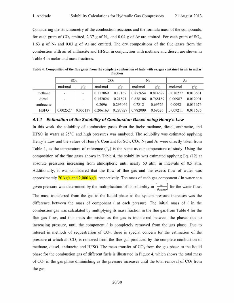
Considering the stoichiometry of the combustion reactions and the formula mass of the compounds,

for each gram of CO2 emitted, 2.37 g of N2, and 0.04 g of Ar are emitted. For each gram of SO2,

1.63 g of N2 and 0.03 g of Ar are emitted. The dry compositions of the flue gases from the

combustion with air of anthracite and HFSO, in conjunction with methane and diesel, are shown in

Table 4 in molar and mass fractions.

Table 4: Composition of the flue gases from the complete combustion of fuels with oxygen contained in air in molar

fraction

SO2 CO2 N2 Ar

mol/mol g/g mol/mol g/g mol/mol g/g mol/mol g/g

methane - - 0.117069 0.17169 0.872654 0.814629 0.010277 0.013681

diesel - - 0.152024 0.21891 0.838106 0.768189 0.00987 0.012901

anthracite - - 0.2096 0.293064 0.7812 0.69526 0.0092 0.011676

HSFO 0.002527 0.005137 0.206163 0.287927 0.782099 0.69526 0.009211 0.011676

4.1.1 Estimation of the Solubility of Combustion Gases using Henry’s Law

In this work, the solubility of combustion gases from the fuels: methane, diesel, anthracite, and

HFSO in water at 25°C and high pressures was analysed. The solubility was estimated applying

Henry’s Law and the values of Henry’s Constant for SO2, CO2, N2 and Ar were directly taken from

Table 1, as the temperature of reference (T̀ ) is the same as our temperature of study. Using the

composition of the flue gases shown in Table 4, the solubility was estimated applying Eq. (12) at

absolute pressures increasing from atmospheric until nearly 60 atm, in intervals of 0.5 atm.

Additionally, it was considered that the flow of flue gas and the excess flow of water was

approximately 20 kg/s and 2,000 kg/s, respectively. The mass of each gas component � in water at a

given pressure was determined by the multiplication of its solubility in G :(:±./²�I for the water flow.

The mass transferred from the gas to the liquid phase as the system pressure increases was the

difference between the mass of component � at each pressure. The initial mass of � in the

combustion gas was calculated by multiplying its mass fraction in the flue gas from Table 4 for the

flue gas flow, and this mass diminishes as the gas is transferred between the phases due to

increasing pressure, until the component � is completely removed from the gas phase. Due to

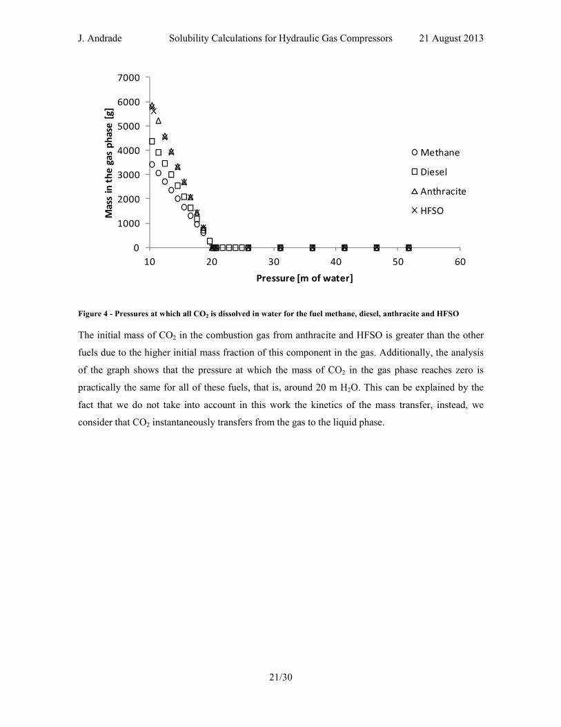
interest in methods of sequestration of CO2, there is special concern for the estimation of the

pressure at which all CO2 is removed from the flue gas produced by the complete combustion of

methane, diesel, anthracite and HFSO. The mass transfer of CO2 from the gas phase to the liquid

phase for the combustion gas of different fuels is illustrated in Figure 4, which shows the total mass

of CO2 in the gas phase diminishing as the pressure increases until the total removal of CO2 from

the gas.


21/30

Figure 4 - Pressures at which all CO2 is dissolved in water for the fuel methane, diesel, anthracite and HFSO

The initial mass of CO2 in the combustion gas from anthracite and HFSO is greater than the other

fuels due to the higher initial mass fraction of this component in the gas. Additionally, the analysis

of the graph shows that the pressure at which the mass of CO2 in the gas phase reaches zero is

practically the same for all of these fuels, that is, around 20 m H2O. This can be explained by the

fact that we do not take into account in this work the kinetics of the mass transfer, instead, we

consider that CO2 instantaneously transfers from the gas to the liquid phase.

0

1000

2000

3000

4000

5000

6000

7000

10 20 30 40 50 60

Ma

ss i

n t

he

ga

s p

ha

se [

g]

Pressure [m of water]

Methane

Diesel

Anthracite

HFSO


22/30

5 Approximation of the vapour-liquid equilibrium of carbon dioxide in water

The solubility of carbon dioxide in water has been calculated at 50°C, because the experimental

data available in the literature are more abundant at this temperature, and the pressure range

analysed was from 1 atm until 60 atm.

5.1 Estimating the solubility of CO2 in water using Henry’s Law

Figure 5 - Solubility of CO2 in water at 50°C obtained applying Henry's Law

The solubility of CO2 in water has been estimated using Henry’s Law following the concepts

discussed in Section 2.2 and Figure 5 above correlates the solubility of CO2 with the system’s

absolute pressure. To predict Henry’s Constant at 50°C, the vant’t Hoff expression (Eq. 13) was

used with the parameters for CO2 presented in Table 1. The simulations were performed using

Excel, assuming infinite dilution, because the flow of H2O (20,000 kg/s) was much higher than the

gas flow (20 kg/s), and that the gas phase has initially the properties of pure CO2, because the

amount of H2O in the CO2-rich phase is reduced at temperatures below 100°C. [20] The solubility

of CO2 in water in mass concentration G :³©v:±./²�I was calculated using Eq. (12) and it could be

modified to molar concentration by using Equation (31).

0

0.005

0.01

0.015

0.02

0.025

0 10 20 30 40 50 60 70

So

lub

ilit

y [

mo

l C

O2

/m

ol

H2

O]

Pressure [atm]


23/30

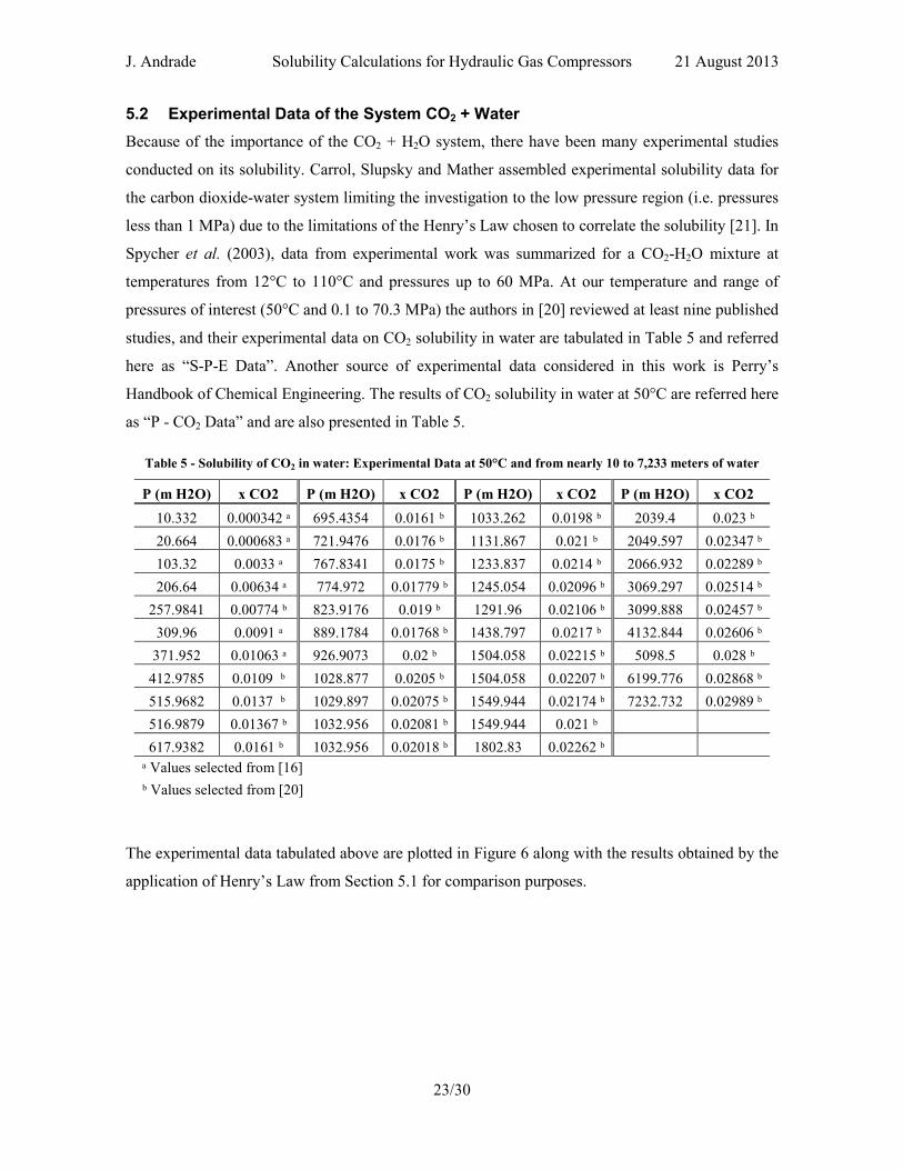
5.2 Experimental Data of the System CO2 + Water

Because of the importance of the CO2 + H2O system, there have been many experimental studies

conducted on its solubility. Carrol, Slupsky and Mather assembled experimental solubility data for

the carbon dioxide-water system limiting the investigation to the low pressure region (i.e. pressures

less than 1 MPa) due to the limitations of the Henry’s Law chosen to correlate the solubility [21]. In

Spycher et al. (2003), data from experimental work was summarized for a CO2-H2O mixture at

temperatures from 12°C to 110°C and pressures up to 60 MPa. At our temperature and range of

pressures of interest (50°C and 0.1 to 70.3 MPa) the authors in [20] reviewed at least nine published

studies, and their experimental data on CO2 solubility in water are tabulated in Table 5 and referred

here as “S-P-E Data”. Another source of experimental data considered in this work is Perry’s

Handbook of Chemical Engineering. The results of CO2 solubility in water at 50°C are referred here

as “P - CO2 Data” and are also presented in Table 5.

Table 5 - Solubility of CO2 in water: Experimental Data at 50°C and from nearly 10 to 7,233 meters of water

P (m H2O) x CO2 P (m H2O) x CO2 P (m H2O) x CO2 P (m H2O) x CO2

10.332 0.000342 ᵃ 695.4354 0.0161 ᵇ 1033.262 0.0198 ᵇ 2039.4 0.023 ᵇ

20.664 0.000683 ᵃ 721.9476 0.0176 ᵇ 1131.867 0.021 ᵇ 2049.597 0.02347 ᵇ

103.32 0.0033 ᵃ 767.8341 0.0175 ᵇ 1233.837 0.0214 ᵇ 2066.932 0.02289 ᵇ

206.64 0.00634 ᵃ 774.972 0.01779 ᵇ 1245.054 0.02096 ᵇ 3069.297 0.02514 ᵇ

257.9841 0.00774 ᵇ 823.9176 0.019 ᵇ 1291.96 0.02106 ᵇ 3099.888 0.02457 ᵇ

309.96 0.0091 ᵃ 889.1784 0.01768 ᵇ 1438.797 0.0217 ᵇ 4132.844 0.02606 ᵇ

371.952 0.01063 ᵃ 926.9073 0.02 ᵇ 1504.058 0.02215 ᵇ 5098.5 0.028 ᵇ

412.9785 0.0109 ᵇ 1028.877 0.0205 ᵇ 1504.058 0.02207 ᵇ 6199.776 0.02868 ᵇ

515.9682 0.0137 ᵇ 1029.897 0.02075 ᵇ 1549.944 0.02174 ᵇ 7232.732 0.02989 ᵇ

516.9879 0.01367 ᵇ 1032.956 0.02081 ᵇ 1549.944 0.021 ᵇ

617.9382 0.0161 ᵇ 1032.956 0.02018 ᵇ 1802.83 0.02262 ᵇ

ᵃ Values selected from [16]

ᵇ Values selected from [20]

The experimental data tabulated above are plotted in Figure 6 along with the results obtained by the

application of Henry’s Law from Section 5.1 for comparison purposes.


24/30

Figure 6 - Solubility of CO2 in water at pressure ranging from 0 to nearly 1,500 meters of water: Results from the

Application of Henry's Law and S-P-E [20] and P-CO2 [16] Experimental Data

The graph shows that Henry’s Law predicts well the solubility of CO2 in water in the range of

pressures from atmospheric until approximately 300 m H2O. Considering that for hydraulic gas

compressors, from Section (4.1.1.), the estimated pressure at which all CO2 from combustion gases

would be completely dissolved in water was approximately 202.65kPa (20.65 m H2O), the

prediction of CO2 solubility in water using Henry’s Law seems acceptable.

5.3 Estimating the solubility of CO2 in water using the VR Therm

Due to the limitations of Henry’s law to predict equilibrium data at high pressure, the solubility of

CO2 in water was also predicted using cubic Equations of State for more precise results. Since the

application of these EoS requires interactive mathematical procedures, the software program,

VRTherm, was used as an add-in to Excel to determine the equilibrium properties of the system.

VRTherm is a library program that can predict thermodynamic properties and physical properties of

complex mixtures, and can be downloaded at <www.vrtech.com.br>. VRTherm can calculate the

fraction of vaporization, the composition of the liquid phase and vapor phase composition, given the

overall composition of the input stream, and the temperature and pressure of the equilibrium. In

VRTherm several Equations of State are available, including Soave-Redlich-Kwong and Peng-

Robinson, presented in this work as Eq. (22) and Eq. (23). Flash calculations were performed using

these two EoS and, in Figure 7, the composition of the liquid phase as a function of the absolute

0

0.005

0.01

0.015

0.02

0.025

0 200 400 600 800 1000 1200 1400 1600

So

lub

ilit

y [

mo

l C

O2

/m

ol

wa

ter]

Pressure [m H2O]

S-P-E Data

P-CO2 Data

Henry's Law Results


25/30

pressure of the system is shown. The results from VRTherm were less accurate than the results

obtained from using Henry’s Law.

Figure 7 - Solubility of CO2 in water predicted from SKR EoS and PR EoS, using VRTherm software, compared

with the S-P-E Experimental Data

5.4 Limitations of Henry’s Law in predicting the solubility of the system CO2 + Water

The carbon dioxide-water system is of great scientific and technological importance. The solubility

of carbon dioxide (CO2) in water (H2O) is one of the most often studied phenomena in all physical

chemistry; however, the dissimilarity between the molecules makes the phase relations in the

system quite complex and the CO2 + water system is highly non-ideal. [4] This dissimilarity is

mainly due to the fact that H2O is small and dipolar whereas CO2 (in the gaseous state) is large and

non-polar; therefore, the miscibility of the components in the liquid phase is extremely low. At low

temperatures, the molecules do not mix, and the two liquids are independently stable– one rich in

CO2 and the other in H2O. The solubility rises with increasing temperature until 265°C and at

approximately 220 MPa when mutual solubility is complete.

CO2 is more volatile than H2O. CO2 has its triple point located at low pressure and temperature (0.5

MPa and -56.6°C) and its critical point at high pressure and approximately at room temperature (7.4

MPa and 31.1°C); whereas, the triple point of H2O is at 0.01°C and at very low pressure (0.0006

MPa) and its critical point is at high pressure and temperature (374°C and 22.1 MPa) [4].

0

0.005

0.01

0.015

0.02

0.025

0 200 400 600 800 1000

So

lub

ilit

y [

mo

l C

O2

/m

ol

wa

ter]

Pressure [m of water]

S-P-E

PR

SRK


26/30

In addition, partitioning occurs, in which CO2 quickly forms hydrated carbon dioxide in water and

then dissociates as carbonic acid (H2CO3). However, the kinetics of these reactions are not taken

into account when using Henry’s Law.

Moreover, some errors in this study can arise due to the effects of electrolytes. It is known that

dissolved solids affect the phase portioning of H2O and CO2; therefore, further studies are necessary

to investigate the impact of dissolved solids on the mutual solubility of CO2 and H2O. [20]

5.5 Estimating the solubility of CO2 in water using the model of Diamond (2003)

Diamond and Akinfiev (2003) evaluated twenty five experimental measurements of the solubility of

CO2 in pure water from 0.1 to 100 MPa. The reliable experimental data were separated from the

unreliable data using the criteria presented in [22] and were correlated by a basic thermodynamic

model based on Henry’s Law and on new high-accuracy EoS. The performance of this model was

evaluated and it is reasonable to consider the activity coefficient of aqueous CO2 equal to one up to

solubilities of nearly 2 mol%. At higher solubilities, the activity coefficients are greater than unity

at low temperatures, and lower than unity at high temperatures. The authors applied an empirical

correlation function for this trend to the basic model and the resulting modified model describes the

accepted data with a 2% level of precision . The corrected model is available as a computer code at

< http://www.geo.unibe.ch/diamond> and, using it in this work, the solubility of CO2 in water at

50°C and from 1 atm to 60 atm was estimated. The results are referred as “D-A Data” and are

shown in Figure 8, in conjunction with the S-P-E and P-CO2 experimental data.

The application of the model from Diamond and Akinfiev is suitable for the estimation of the

solubility of CO2 in pure water from 1 to 60 atm, due to the increased precision of the results when

compared with experimental data.


27/30

Figure 8 - CO2 solubility in water at 50°C using the model from [22] referred as D-A Data in comparison with S-P-

E and P-CO2 experimental data

0

0.005

0.01

0.015

0.02

0.025

0 200 400 600 800 1000

So

lub

ilit

y [

mo

l C

O2

/m

ol

wa

ter]

Pressure [m H2O]

S-P-E Data

P-CO2 Data

D-A Data


28/30

6 Conclusions

Despite recent efforts to predict the solubility of gases at high pressures, there are insufficient

results in the literature, many of which are imprecise. This work focused on the estimation of air

and combustion gases solubility in pure water with the aim to update hydrodynamic calculations for

hydraulic gas compressors.

The solubility of air components in water was shown to be precisely estimated via the utilization of

Henry’s Law, either using either the van’t Hoff expression or Kolev’s correlations, when compared

with reliable experimental data from the literature. As expected, due to the higher solubility in

water, argon is the first component that is completely dissolved in water, followed by O2 and N2.

The solubility of combustion gases produced from anthracite, methane, HFSO and diesel were also

estimated using Henry’s Law, however, by neglecting the kinetics associated with the mass transfer

from the gas to the liquid phase, the pressure at which the combustion gases would be totally

dissolved was almost the same for all fuels studied.

However, the application of Henry’s Law to estimate the solubility of CO2 in water was shown to

be inadequate at pressures higher than 20 atm; moreover, the use of the program VRTherm led to

results far from the experimental measurements. The application of the model proposed by

Diamond and Akinfiev was the most suitable for the estimation of CO2 solubility in water from 1 to

60 atm.


29/30

7 References

[1] Wilhelm E, Battino R, Wilcock R J. (1977). Low-Pressure Solubility of Gases in Liquid Water.

Chemical Reviews. 77 (2), 219-262.

[2] Mutoru J W,Leahy-Dios A, Firoozabadi A. (2011). Modeling infinite dilution and Fickian

diffusion coefficients of carbon dioxide in water. AIChE Journal. 57 (6), 1617-1627.

[3] Chen L, Rice W. (1983). Properties of air leaving a Hydraulic Air Compressor (HAC). J. of

Energy Resources Technology. 105 (55), 54-57.

[4] Diamond L W. (2001). Review of the systematics of CO2-H2O fluid inclusions. Lithos. 55, 69-

99.

[5] Pedersen K S, Christensen P L. (2007). Phase Behavior of Petroleum Reservoir Fluids. Boca

Raton, FL, USA: CRC Press (Taylor & Francis).

[6] Skogestad S. (2009). Chemical and Energy Process Engineering. CRC Press (Taylor and

Francis). 179-196.

[7] Battino R, Clever H L (1966). The Solubility of Gases in Liquids. Chemical Reviews. 66 (3),

395-463.

[8] Smith F L, Harvey A H (2007). Avoid Common Pitfalls When Using Henry's Law. In: Chemical

Engineering in Progress (CEP) Magazine. 33-39, http://www.aiche.org/resources/publications/cep

[9] Sander R. (1999). Compilation of Henry’s Law Constants for Inorganic and Organic Species of

Potential Importance in Environmental Chemistry. Air Chemistry Department; Max-Plank Institute

of Chemistry. Available: http://www.mpch-mainz.mpg.de/~sander/res/henry.html. Last accessed

14th Aug 2013.

[10] Smith J M, Van Ness H C (1987). Introduction to Chemical Engineering Thermodynamics. 4th

ed. United States of America: McGraw-Hill Book Company.

[11] Kontogeorgis G M, Economou I G. (2010). Equations of state: from the ideas of van der Waals

to association theories. J. of Supercritical Fluids. 55, 421-437.

[12] Finlayson B A (2006). Introduction to Chemical Engineering Computing. Hoboken, New

Jersey: John Wiley & Sons, Inc.. 25-40.

[13] Abudour A M, Mohammad S A, Gasem K A M. (2012). Modeling high-pressure phase

equilibria of coalbed gases/water mixtures with the Peng-Robinson equation of state. Fluid Phase

Equilibria. 319, 77-89.

[14] Kolev N I (2007). Multiphase Flow Dynamics 3. Turbulence, Gas Absorption and Release,

Diesel Fuel Properties. Springer. 185-214.

[15] Battino R, Rettich T R, Tominaga T. (1984). The Solubility of Nitrogen and Air in Liquids. J.

Phys. Chem. 13 (2), 563-600.

[16] Maloney J O (2008). Perry’s Chemical Engineers' Handbook. 8th ed. McGraw-Hill Book

Company.

[17] ASTM E176-04, Standard Terminology of Fire Standards, ASTM International, W.

Conshohocken, PA, 2004.

[18] International Association of Independent Tanker Owners (INTERTANKO). Review of the CO2

operational index. In: Intersessional Meeting of The Greenhouse Gas Working Group; International

Maritime Organization, http://www.sjofartsverket.se/pages/16278/1-3-1.pdf; 2008.


30/30

[19] Ouyang Z, Zhu J, Lu Q. (2013). Experimental Study on preheating and combustion

characteristics of pulverized anthracite coal. Fuel. 113, 122-127.

[20] Spycher N, Pruess K, Ennis-King J. (2003). CO2- H2O mixtures in the geological sequestration

of CO2. Assessment and calculation of mutual solubilities from 12 to 100°C and up to 600 bar.

Geochimica and Cosmochimica Acta. 67 (16), 3015–3031.

[21] Carroll J J, Slupsky J D, Mather A E (1991). The Solubility of Carbon Dioxide in Water at

Low Pressure. J. Phys. Chem.. 20 (6), 1201-1209.

[22] Diamond L W, Akinfiev. (2003). Solubility of CO2 in water from -1.5 to 100°C and from 0.1

to 100 MPa: evaluation of literature data and thermodynamic modeling. Fluid Phase Equilibria.

208, 265-290.

julia andrade - solubility calculations for hydraulic gas ... · pdf filej. andrade solubility...

Documents