AN ABSTRACT OF THE THESIS OF

Michele Meadows Dailey for the degree of Master of Science in Geography presented on November 30, 2007. Title: Meadow Classification in the Willamette National Forest and Conifer Encroachment Patterns in the Chucksney-Grasshopper Meadow Complex, Western Cascade Range, Oregon. Abstract approved:

Julia A. Jones This study delineates and characterizes the distribution of montane meadows in the

Willamette National Forest, identifies encroachment patterns in relation to

topographic features and proximity to trees in the Chucksney-Grasshopper meadow

complex, and examines tree species and age distributions in relation to distance from

forest edges or isolated tree clusters in the West Middle Prairie meadow.

The Willamette National Forest covers approximately 6780 km2 and intersects two

main physiographic provinces comprised of the Cascade Crest Montane Forests and

Subalpine/Alpine regions to the east, and the Western Cascades Montane, Lowland,

and Valley regions to the west. Tree species commonly found in the study area

include firs, cedar, pine, larch, spruce, and hemlock. Non-forested openings,

including meadows, are distributed throughout the study area. Matched Filtering

analysis was applied to Landsat ETM+ imagery acquired in September 2002 and

combined with ancillary data that delineates stand replacing fire and harvest

disturbances that occurred between 1972 and 2004 to create a vegetation

classification of the Willamette National Forest that identifies meadows. The

meadow classification was then combined with data depicting topographic position,

slope, aspect, and elevation. Chi-squared statistics were applied to determine if

meadows were significantly concentrated in areas characterized by these physical

factors. In the western extent of the Willamette National Forest, meadows are

concentrated on steep, south and east facing ridges between 1000 and 2000m in

elevation. In the eastern extent of the Willamette National Forest, meadows are

concentrated in valleys between 500 and 1000 meters in elevation and occur on both

gentle and steep, east and south facing slopes. The vegetation classification provides

a consistent and comprehensive dataset of meadow distribution in the Willamette

National Forest.

The Chucksney -Grasshopper meadow complex is contained by the Chucksney

Mountain roadless area and comprised of approximately 8 distinct meadows located

27 kilometers northeast of Oakridge in the Willamette National Forest. The meadows

occur on mostly south and east facing steep slopes near the ridgeline, and host varied

dry and mesic plant communities. Herbaceous cover for three snapshots in time was

classified using aerial photographs taken in 1947, 1972, and 2005 to determine

conifer encroachment into the meadows. Chi-squared statistics were applied to

determine if encroachment patterns were associated with slope, aspect, or proximity

to tree cover. Encroachment occurred significantly closer to existing trees in all

meadows suggesting the ameliorating effects of forest create conditions favorable for

seedling establishment. Encroachment was also significant on steep, south and east

facing slopes in some meadows, but also on gentle, west facing slopes in other

meadows indicating a complex interaction of land use history, physical, and

biological factors. The encroachment history analysis provides the preliminary

framework for a model that can be used to identify meadows at risk for invasion.

The West Middle Prairie of the Chucksney-Grasshopper complex, also known as

Meadow 4, is a 21 hectare meadow characterized by a dry meadow community at the

northern boundary, a mesic forest-meadow mosaic towards the southern boundary,

and a rock garden at the western boundary. This meadow underwent mechanical tree

removal in 1964 and a prescribed burn in 1996 to thwart conifer invasion. Four

transects intersecting burned and unburned areas at the forest edge and through

isolated tree clusters were sampled to determine the distribution of tree species and

ages relative to their position in the transect. Data imply Pinus contorta invasion was

promoted by the 1996 burns and that seedling establishment has occurred

progressively from forest edges as well as simultaneously in a band along the forest

edge. These findings suggest the prescribed burn was not adequate to control

invasion and such management methods should be reviewed in the context of on-

going research into alternate eradication measures. This research also supports other

work that suggests initial seedling establishment accelerates subsequent seedling

establishment and that eradication of early invaders is important for efficient

management.

This study can inform meadow habitat maintenance and restoration in three ways:

it provides and inventory of meadows in the Willamette National Forest, a framework

for a tool to predict which meadows are at risk for invasion and therefore are potential

targets for action, and finally a report on past maintenance efforts and observation of

invasion patterns at a fine scale.

© Copyright by Michele Meadows Dailey November 30, 2007 All Rights Reserved

Meadow Classification in the Willamette National Forest and Conifer Encroachment Patterns in the Chucksney-Grasshopper Meadow Complex, Western Cascade Range,

Oregon

by Michele Meadows Dailey

A THESIS

Submitted to

Oregon State University

in partial fulfillment of the requirements for the

degree of

Master of Science

Presented November 30, 2007 Commencement June 2008

Master of Science thesis of Michele Meadows Dailey presented on November 30, 2007. APPROVED: Major Professor, representing Geography Chair of the Department of Geosciences Dean of the Graduate School I understand that my thesis will become part of the permanent collection of Oregon State University libraries. My signature below authorizes release of my thesis to any reader upon request.

Michele Meadows Dailey, Author

ACKNOWLEDGEMENTS

There are many people to acknowledge for their help, inspiration, and support but

perhaps none more so than Dr. Julia Jones, my major advisor. She asked me the most

simple, yet profound question: “Where do you like to be?” The answer led me to this

thesis topic and the recognition of the importance of place, not only to a geographer,

but to any person trying to understand nature. Dr. Jones also gave me great personal,

intellectual, and monetary support for which I am very grateful.

The remainder of my committee should also be acknowledged for their important

roles in my Masters’ experience. Dr. Anne Nolin, my minor advisor, has served as a

great mentor and educator. I appreciate her high standards and interest in her

students’ success. I am also grateful for her robust editing and advising for the

remote sensing chapter of this thesis. Thank you to Dr. Jon Kimerling for serving on

my committee as well as for impromptu swing dance lessons and a wonderful and

boisterous presence. And finally, thank you to Anthony Koppers for serving as my

Graduate Council Representative.

Countless others helped me complete my research. Dr. Dawn Wright provided

funding and opportunities for which I am very grateful. Charlie Halpern, Fred

Swanson, Warren Cohen, Janine Rice, Alan Tepley, Cheryl Friesen, Jennifer Lippert,

and Jim Kiser generously and kindly imparted their wisdom and resources upon me.

Maureen Duane and the staff of the H.J. Andrews facilitated my data hunting and first

“practice” field season. Mark Meyers provided lab support. Finally, my field

assistants protected me from mountain lions, mosquitoes, and long lonely days in the

field as well as helped do hard labor. Thank you to Mark Bernard, Biniam Iyob, Quin

Ourada, Bronwen Rice, Nate Shaub, and Jam the dog.

The Geosciences staff and friends encouraged and supported me, helping me

through my times of doubt and frustration. I’m so glad you were there: Marion

Anderson, Aaron Arthur, Katherine Hoffman, Kyle Hogrefe, Melinda Peterson,

Bronwen Rice, Jed Roberts, Emily Underwood, Joanne Van Geest and the rest of the

A-team.

TABLE OF CONTENTS

Page 1 Introduction ………………………………………………………..………………1 2 Previous Research ………………………………………………………………....5 3 A Remote Sensing Classification of Non-Forest Openings in the Willamette National Forest ………………………………………………………...…………13 3.1 Introduction and Objectives ………………………...…….……….……13 3.2 Study Area ………………………………………………….……..……13 3.2.1 Geology and Topography …………………………………….14 3.2.2 Climate ………………………………….……….……………15 3.2.3 Soils …………………………………………….……….……16 3.2.4 Rivers/Basins …………………….……………..…………….17 3.2.5 Vegetation …………….…………………………..…………..18 3.2.6 Fauna …………………………………………….……………23 3.2.7 Land Use History ……………………………………………..23 3.2.8 Current Land Cover/Land Use ………………………..….…...27

3.3 Methods …………………………………………………..…….………32 3.3.1 Data Description ………………………………………...……33

3.3.2 Image Processing ………………………………..……………34 3.3.3 GIS Analysis …………………………………………….……52 3.4 Results …………………………………………………..……..………..66 3.4.1 Results of Image Processing …………………..……...………66 3.4.2 Results of GIS Analysis ………………………..….….………72 3.5 Discussion ……………………………………………………..……..…84 4 Change in the Chucksney-Grasshopper Meadow Complex, 1947-2005 …….…..91 4.1 Introduction and Objectives …………….………………………………91 4.2 Study Area …………….………………………………………………..91 4.2.1 Geology ……………………….…………………………….…93 4.2.2 Climate ……………………………………………….………..94 4.2.3 Soils ………………………………………………….………..94 4.2.4 Rivers/Basins ………………………………………….………95 4.2.5 Vegetation ……………………………………………….…….96 4.2.6 Fauna …………………………………………………………..97 4.2.7 Land Use and Management History …………………………..97 4.2.8 Current Land Use ………………………………..……….…..105 4.3 Methods ……………………………….……………………………….106

4.3.1 Data Description ……………………………………………..106 4.3.2 Image Processing …………………………………………….106 4.3.3 GIS Analysis ………………………………………..………. 107

TABLE OF CONTENTS (Continued)

Page 4.4 Results ……………………………………………………….…...……112 4.4.1 Results of Image Processing ………………………………....112 4.4.2 Results of GIS Analysis …………………………… ………..119 4.5 Discussion ……………………………………………….………….…129 5 Tree Invasion Along Forest-Meadow Transects in the Chucksney-Grasshopper Meadow Complex, Western Cascade Range of Oregon……………………..….134 5.1 Introduction and Objectives ……………………………….…………..134 5.2 Background …………………………………………….……...………134 5.2.1 Abies concolor var. lowiana …………………………………135 5.2.2 Abies grandis ………………………………………….……..136 5.2.3 Pinus contorta …………………………………….…….……138 5.2.4 Pseudotsuga menziesii …………………………………….…140

5.2.5 Thuja plicata …………………………………………………141 5.4.6 Tsuga heterophylla……………………………………………143 5.3 Study Area ……………………….……………….………….………. 144 5.4 Methods ..…………………...……..…………….………….………….146 5.5 Results……………….………………………….……..…….…………148 5.6 Discussion ……………………………….……………………...……. 181 6 Conclusion……………………………………………...……………………….186

Literature Cited …………………………………………………………………….190

LISTS OF FIGURES

Figure Page 3.1 Location of Willamette National Forest within the Oregon Western

Cascades physiographic province ………………………………………..….14 3.2 Location of the Western Cascades within hydrological sub-regions

and location of the WNF within river sub-basins …………………….……..18 3.3 Major vegetational zones of the Oregon western Cascade Range ………….…..32 3.4 Cohen et al. (1988) Land Cover of Western Oregon data, clipped to the WNF study area extent and projected forward to reflect current stand ages ……………………………………………………………………..….. 29 3.5 Cohen and Lennartz (2004) Stand Replacement Disturbance data clipped to the WNF study area extent………………………………….……………..31 3.6 WNF administrative and study area boundaries compared ………………….…33 3.7 2005 photograph of meadow, outlined in yellow, comprised of herbaceous, vegetation, shrub, and tree cover near Grasshopper Mountain ………………………………………………………………….…36 3.8 Thirty meter grid superimposed over an aerial image of a portion of

the study area, demonstrating potential proportion of herb, shrub, or tree within each 30-m pixel ……………………………………….37

3.9 Landsat ETM+ spectral profiles of meadow, forest, and shrub endmembers. ………………………………………………………………..38 3.10 Flow chart of endmember classification decision process based on

endmember values compared to each other and aerial photography ………..41 3.11 2005 aerial photograph and Cohen et al.’s 1988 forest vegetation (vegmap) classification of the Grasshopper Mountain meadow, demonstrating the vegmap classification of herbaceous vegetation as 30-70% cover. ……………………………………………………….….. 43 3.12 Cohen and Lennartz 2004 stand replacing disturbance dataset and the vegetation classification of the Grasshopper meadow, demonstrating the disturbance dataset’s classification of meadow as “forest no-change”…………………………………………...………………44

LIST OF FIGURES (Continued) Figure Page 3.13 Two maps of the same extent comparing the Cohen and Lennartz

Disturbance dataset and the vegetation classification demonstrating the misclassification of regenerating clear cuts as meadow in the vegetation classification …………………………………………………….48

3.14 Topographic position model output for Oregon western Cascade Range ….....55

3.15 Topographic position model output for Chucksney-Grasshopper meadow complex area ………………………………………….……………56 3.16 Example of meadow/barren class from final classification

combined with topographic position output at Grasshopper Ridge …………………………………………………………….…….…….57

3.17 Five-hundred meter increment elevation bands for WNF ……………….…....59

3.18 Eight classes of slope in degrees for the WNF ……………………………….61

3.19 Aspect reclassified into eight cardinal directions at Chucksney- Grasshopper ………………………………………………………....………63

3.20 EPA Level IV Ecoregion designations of western Cascade Range

and WNF boundary…………………………………………………………..65

3.21 Final land cover classification of WNF study area incorporating vegetation classification and Cohen and Lennartz 2004 disturbance data …………………………………………………………………………..67

3.22 Distribution of meadow class by topographic position normalized by distribution of the WNF by topographic position for the WNF-west extent ……………………………………………………...…….73 3.23 Distribution of meadow class by topographic position normalized by distribution of the WNF by topographic position for the WNF-east extent……………………………………………………………..75 3.24 Distribution of meadow class by elevation band normalized by distribution of the WNF by elevation band for the WNF-west extent ……………………………………………………………………...…76

LIST OF FIGURES (Continued) Figure Page 3.25 Distribution of meadow class by elevation band normalized by distribution of the WNF by elevation band for the WNF-east extent …………………………………………………………………...……78 3.26 Distribution of meadow class by slope in degrees class normalized by distribution of the WNF by slope in degrees class for the WNF-west extent ……………………………………………………...…….79 3.27 Distribution of meadow class by slope in degrees class normalized by distribution of the WNF by slope in degrees class for the WNF-east extent ………………………………………………………….…81 3.28 Distribution as percent of meadow class by aspect class and distribution as percent of the WNF by aspect class for the WNF-west extent …………………………………………..………………. 82 3.29 Distribution as percent of meadow class by aspect class and distribution as percent of the WNF by aspect class for the WNF-east extent.………………………………………...…………………..84 4.1 Location of the Chucksney – Grasshopper complex within the

Chucksney Mountain Roadless Area …………………………..……………92

4.2 Geology of the Chucksney-Grasshopper meadow complex …………...………93 4.3 Sub-watersheds of the Chucksney-Grasshopper meadow

complex area ………………………………………………...………………96 4.4 Photograph of the Grasshopper Meadow (Meadow 1) after the

fall 2007 burn …………………………………………………...………….102 4.5 Photograph of historic grazing trenches that were revealed in

Meadow 1 when 2007 fire removed vegetative cover …………………..…103 4.6 Photograph of trees in Meadow 1 that were felled in 2006

and burned in 2007 ……………………………………………………..…..104 4.7 Photograph of patchy 2007 burn in Meadow 1 with historic water

trough at center ……………………………………………………...……..105 4.8 Extent of meadow/barren class (shown as pale yellow) in Meadow 1 over 1947, 1972, and 2005 photographs ………………………………...…114

LIST OF FIGURES (Continued) Figure Page 4.9 Extent of meadow/barren class (shown as pale yellow) in Meadow 2 over 1947, 1972, and 2005 photographs.………………………………...…115 4.10 Extent of meadow/barren class (shown as pale yellow) in Meadow 3 over 1947, 1972, and 2005 photographs.…………………………………...116 4.11 Extent of meadow/barren class (shown as pale yellow) in Meadow 4 over 1947, 1972, and 2005 photographs.………………………………..….117 4.12 Extent of meadow/barren class (shown as pale yellow) in Meadows 5 and 6 over 1947, 1972, and 2005 photographs.…………………………….118 4.13 Extent of meadow/barren class (shown as pale yellow) in Meadows 7 and 8 over 1972 and 2005 photographs.……………………………………119 5.1 2005 photograph of Meadow 4 ……………………………..…………..…….144

5.2 Location of survey transects within Meadow 4 ………………………...…….147

5.3 Orientation and designation of survey blocks for Transect T1 ……...………..150

5.4 Age of trees by species in relation to the distance from the end of the transect closest to the forest in Transect 1 ……………………….….153 5.5 Orientation and designation of survey blocks for Transect T2 ……………….154 5.6 Age of trees by species in relation to the distance from the downslope end of Transect 2 ………………………………………………157 5.7 Orientation and designation of survey blocks for Transect T3 …………….....158 5.8 Age of trees by species in relation to the distance from the forested end of Transect 3 ………………………………………...………..161 5.9 Orientation and designation of survey blocks for Transect T4 ……….……….162 5.10 Age of trees by species in relation to the distance from the forested end of Transect 4.…………………………………………...……..167 5.11 Plot of relationship between age and dbh (cm) for all Abies grandis samples ………………………………………………...………….168

LIST OF FIGURES (Continued) Figure Page 5.12 Plot of relationship between age and dbh (cm) for Abies grandis samples taken from Transect 2.…………………………...………168 5.13 Plot of relationship between age and dbh (cm) for Abies grandis samples taken from Transect 3 ……………………………….…..169 5.14 Plot of relationship between age and dbh (cm) for Abies grandis samples taken from Transect 4 ……………………………...……169 5.15 Plot of relationship between age and dbh (cm) for all Pinus Contorta samples taken …………………………………….………………170 5.16 Plot of relationship between age and dbh (cm) for Pinus contorta samples taken in Transect 1 ………………………………………171 5.17 Plot of relationship between age and dbh (cm) for Pinus contorta samples taken in Transect 3 …………………………………...….171 5.18 Plot of relationship between age and dbh (cm) for all Pseudotsuga menziesii samples taken ……………………………………………...…….172 5.19 Plot of relationship between age and dbh (cm) for Pseudotsuga menziesii samples taken in Transect 3 …………………………………..…173 5.20 Plot of relationship between age and dbh (cm) for Pseudotsuga menziesii samples taken in Transect 4 ……………………………….…….173 5.21 Plot of relationship between age and dbh (cm) for all Thuja plicata samples taken ……………………………………………………………....174 5.22 Plot of relationship between age and dbh (cm) for all Tsuga heterophylla samples taken ……………………………………………...…175 5.23 Plot of relationship between age and dbh (cm) for Tsuga heterophylla samples taken in Transect 3 …………………….…….……..175 5.24 Plot of relationship between age and dbh (cm) for Tsuga heterophylla samples taken in Transect 4 ………………………………...176 5.25 Plot of relationship between snag size and distance from forested end of Transect 4 ……………………………………………………….…..177

LIST OF FIGURES (Continued) Figure Page 5.26 Plot of relationship between seedling occurrence and distance to end of Transect 1 closest to forest edge …………………………………....178 5.27 Plot of relationship between seedling occurrence and distance to downslope end of Transect 2 ……………………………………………179 5.28 Plot of relationship between seedling occurrence and distance to forested end of Transect 3 …………………………………………….....180 5.29 Plot of relationship between seedling occurrence and distance to forested end of Transect 4 …………………………………………….…181

LIST OF TABLES Table Page 3.1 Scientific and common names of commonly found tree

species in Oregon western Cascade Range …………………………...……..19 3.2 Area of the 1988 Land Cover of Western Oregon cover classes projected to 2007 for the portion of this chapter’s study area the original data covers ………………………………………………..…….30 3.3 Area and percent of WNF study area of the Stand Replacement Disturbance classes (1972-2004) ………………………….………….….….32

3.4 Final classification categories and source ……………………………..…….….47

3.5 Percent and area of classes in final classification ………………………………68 3.6 Classification validation error matrix and Producer’s and

User’s accuracies ……………………………………………………………70 3.7 Classification Conditional Khat results per class ………………………………..70 3.8 Results of SHABS polygons being attributed with the majority class of the final classification …………………………………………..…..71 3.9 Area and percent of east and west study areas covered by meadow/barren (meadow) and shrub/very open forest (shrub) classes ……………………………………………………….………72 3.10 Area and percent of WNF and meadow class per

topographic position for the WNF-west extent ……………………….……..73 3.11 Area and percent of WNF and meadow class per

topographic position for the WNF-east extent ………………………………74 3.12 Area and percent of WNF and meadow class per

500m elevation band for the WNF-west extent ……………………….…….76 3.13 Area and percent of WNF and meadow class per

500m elevation band for the WNF-east extent ……………………...………77 3.14 Area and percent of WNF and meadow class per

degree slope class for the WNF-west extent ………………………….……..79

LIST OF TABLES (Continued) Table Page 3.15 Area and percent of WNF and meadow class per

degree slope class for the WNF-east extent …………………...…………….80 3.16 Area and percent of WNF and meadow class per

aspect range for the WNF-west extent ………………………………...…….82

3.17 Area and percent of WNF and meadow class per aspect range for the WNF-east extent ……………………………………….83

4.1 Approximate bounding coordinates and area of Meadows 1 through 6 in 1947 and Meadows 7 and 8 in 1972 ……………………….…..92 4.2 Geo-referencing RMS errors in meters by photo year

and meadow designation ………………………………………..………….107

4.3 Possible encroachment class combinations and outcomes for Meadows 1-6 …………………………………………………..……….109

4.4 Possible encroachment class combinations and outcomes

for Meadows 7-8 …………………………………………………...………109 4.5 Beginning area, percent loss, and change in area of herbaceous cover per meadow per year.………………………………………………...112 4.6 Area and proportion of meadow-only that had/had not experienced encroachment by distance-to-tree category.………………………………..120 4.7 Area and proportion of meadow-only that had/had not experienced encroachment by slope category.…………………………………...………122 4.8 Area and proportion of meadow-only that had/had not experienced encroachment by aspect category.………………………………………….124

4.9 Mean distance to tree of portions of study areas that were encroached by tree cover compared to areas that remained meadow over the period 1947 to 2005 or 1972 to 2005 and Chi squared and p-values describing relationship between the percent encroachment in each meadow per distance-to-tree category and the percent of meadow per category ...……...125

LIST OF TABLES (Continued) Table Page 4.10 Mean degree slopes of portions of study areas that were encroached by tree cover compared to areas that remained meadow over the period 1947 to 2005 or 1972-2005 and Chi squared and p-values describing relationship between the percent encroachment in each meadow per slope category and the percent of the meadow per category …………..…..127 4.11 Mean aspect of portions of study areas that were encroached by tree cover compared to areas that remained meadow over the period 1947 to 2005 or 1972 to 2005 and Chi squared and p-values describing relationship between the percent encroachment in each meadow per aspect category and the percent of the meadow per category …………..….128 5.1 Relative tolerances of dominant species in Meadow 4 to shade and fire ….….135 5.2 Transect T1 field data by survey block ………………………………………..151

5.3 Species codes displayed in data tables with scientific and common names …..152

5.4 Transect T2 field data by survey block ………………………………………..155

5.5 Transect T3 field data by survey block …………………………………..……159

5.6 Transect T4 field data by survey block …………………………………..……163

Meadow Classification in the Willamette National Forest and Conifer Encroachment

Patterns in the Chucksney-Grasshopper Meadow Complex, Western Cascade Range,

Oregon

1 Introduction

Meadows, sometimes called prairies or non-forested openings, are generally

considered to be treeless areas surrounded by forest. They occur on all types of soils,

slopes, and topographic positions. In montane areas, they occur mostly on “steep south-

facing slopes, in small hydric basins, and in areas of flat, but poorly drained topography”

(Miller and Halpern, 1998). In subalpine areas they occur mostly on gentle slopes and in

broad basins, but also on plateaus and high ridges (Miller and Halpern, 1998). Meadow

plant communities vary by geography, site conditions and land use history. In the

Oregon Cascade Range, they are “biological hotspots” supporting a large number of plant

and animal species (Takaoka and Swanson, 2006; Thompson, 2007).

Encroachment into montane meadows by conifers endangers the diversity and

existence of meadow species (Haugo and Halpern, 2007). Most research suggests that

encroachment is caused by a combination of factors including climate change, impacts of

grazing, and disruption of aboriginal and natural fire regimes (Haugo and Halpern, 2007;

Miller and Halpern, 1998; Vale, 1981; Franklin et al., 1971; Takaoka and Swanson,

2006). Land managers have begun to counteract meadow losses with maintenance and

restoration efforts, such as mechanical tree removal and prescribed burning.

2

This research examines meadows in the Willamette National Forest at three scales.

Chapter 3 describes the methods and results of a small scale meadow inventory that was

completed using Landsat ETM+ imagery and GIS analysis that modeled the distribution

of meadows in the Willamette National Forest (WNF). Distribution is characterized by

slope, aspect, elevation, and location within the western or high Cascade Ecoregional

provinces. Chapter 4 examines the methods and results of historic and current photo-

interpretation used to detect medium scale historic meadow encroachment for a complex

of eight meadows in the Chucksney Mountain-Grasshopper Ridge area of the WNF.

Encroachment patterns and rates are analyzed for their relationship to slope, aspect, and

proximity to tree cover. Chapter 5 chronicles the methods and results of a field sampling

exercise in one meadow in the complex used to determine fine scale encroachment

patterns in four transects. Species and age distributions are examined in their relation to

distance from forest edges and isolated tree clusters. The apparent effect of a 1996

prescribed burn on species composition is also examined.

Although meadows have been managed in the Willamette National Forest since at

least the 1960s, the state of geographically referenced data reflects the timber intensive

strategies of the past. Two readily available datasets provide a partial inventory of

meadows and a forest cover class that could potentially identify meadows. However,

neither of these datasets provides a specific and consistent inventory of meadows. The

“Special Habitats” (SHABS) data developed by the WNF (WNF-GIS 2006) provides

polygons of meadow areas for the northern and southern portions of the forest extent.

3

Meadows in the middle portion of the WNF have not been delineated. The 1988 Western

Oregon Composite Forest Vegetation Layer contains a <30% cover class that could

potentially be useful in identifying meadows (Cohen et al., 1988). However, as described

in Chapter 3, it was not appropriate for this purpose.

The Chucksney Mountain-Grasshopper Ridge meadow complex has a complicated

land use history. It was probably burned by Native Americans before white settlers

arrived. Its sheep grazing history is documented in United States Forest Service records.

It has been actively managed for conifer invasion since the 1960s. Historic aerial

photographs from 1947 and 1972 were used in conjunction with 2005 aerial photographs

to delineate a pattern of encroachment in the complex. Though the eight meadows are

relatively similar, they exhibit different rates and patterns of encroachment. These are

examined in Chapter 4.

Meadow 4 in the Chucksney-Grasshopper complex was chosen for field sampling

because of its management history, patterns of tree encroachment, and varied slopes and

vegetation. Mechanical tree removal was conducted in this meadow in 1964 and a

prescribed burn was conducted in 1996. The meadow includes areas where

encroachment has occurred as a wave from the edge or radially from tree islands. It has

areas of dry plant communities on the flatter, though still relatively steep, northern slope

and more mesic communities on the steeper southern slope (Salix, 2005). Field sampling

revealed the chronology of tree establishment and growth rates as well as expected

4

species specific-behaviors related to shade and moisture tolerances based on site

conditions. This meadow also reveals (see Chapter 5) the complexity of trying to isolate

causes of encroachment when drivers are synchronous and the specific history of the

landscape is unknown.

5

2 Previous Research

Virtually all previous research on conifer encroachment into meadows considers two

main drivers: climate change and changes in land use and management. The impacts of

these drivers differ depending on the physical environment occupied by different types of

meadows. The mechanisms by which encroachment occur also depend on physical as

well as biological characteristics.

Climate change affecting tree invasion rates into high-elevation meadows has been

noted to occur as far back as approximately 5,000 years ago. The Absaroka Mountains,

in the Rocky Mountains of Montana and Wyoming, have areas of tree expansion that

occurred during the warmer periods and contractions that occurred during the drier

periods of the mid-Holocene (Jakubos and Romme, 1993). Changes in temperature and

precipitation are not synchronous across all regions, however. Recent climate change in

western North America is thought to have begun when cooler summers ended in the mid

1800s (Dunwiddie, 1977; Jakubos and Romme, 1993). Miller and Halpern (1998) used

precipitation and temperature data compiled by WeatherDisc Associates, Inc. and NOAA

to describe the following climatologic trends in the west-slope Cascades. Mean annual

and mean summer temperatures rose from about 1900 to 1940 while precipitation

remained below average. The period between 1920 and 1945 was unusually warm and

dry. Snow pack was below average during this time as well. The years between 1945

and 1985 remained warm but were wetter than the period of 1920 to 1945. Between

1985 and 1993 temperatures were above average and precipitation dropped to below

6

average (Miller and Halpern, 1998). Increasing spring temperatures have led to

decreased snow pack since the 1970s (Lepofsky et al., 2003). Westerling et al. (2006)

have also associated warming trend in the western US with earlier snowmelts since the

mid-1980s.

Changes in land use and land management are primarily changes in natural or

anthropogenic disturbance regimes. They generally take the form of grazing and fire

suppression. Grazing began in western North America in the late 1800s. Stock included

sheep, cattle and horses. The timing and intensity of grazing varies widely and is species

and site specific. Aboriginal burning of meadows is known to have occurred throughout

the Pacific Northwest. However, oral histories and sparse evidence provide only a vague

account of this practice (Boyd, 1999; French, 1999; Robbins, 1999; Whitlock, 2004,

Lepofsky, 2003). Fire suppression began when European settlers stopped the Native

American practice of burning and continues today with suppression of natural and human

caused wildfires.

Studies have revealed patterns of encroachment based on changes of climate and

disturbance regimes associated with specific physical factors (Franklin et al., 1971;

Dunwiddie, 1977; Vale, 1981; Taylor, 1990; Evans and Fonda, 1990; Jakubos and

Romme, 1993; Miller and Halpern, 1998; Lepofsky et al., 2003; Takaoka and Swanson,

2006; Norman and Taylor, 2005; Coop and Givnish, 2007; Haugo and Halpern, 2007).

Slope gradient, slope aspect, soil moisture, and proximity to forest cover are among those

7

physical factors. Results are as varied as study site characteristics and it is difficult to

tease consistent patterns from these studies. However, Miller and Halpern (1998) note

that patterns and correlates of invasion are similar on sites with similar physiography and

vegetation. Because certain changes in climate and land management occurred

simultaneously, it is not always possible to tell which is responsible for invasion. More

importantly, there usually is not one single driver of conifer invasion but rather a

combination of drivers.

There are some common themes in the reviewed studies. The impact of climate

change depends on the effect it has on length of growing season, temperature extremes,

and soil moisture content and if these factors cause conditions that limit plant growth

when climate change is not a consideration. Topographic gradients are also important

because of their effects on insolation and soil moisture. Meadows created by fire are

more vulnerable to invasion when fire is suppressed than meadows not created by fire.

The type of stock and intensity of grazing impacts the levels of soil disturbance and

seedling damage differently, resulting in different encroachment responses. Finally, the

alteration of the environment by tree establishment not only provides an immediate

benefit to subsequent seedling establishment but can also have long-term effects on

environmental conditions even after tree removal. Specific findings related to these

themes are found in Franklin et al., 1971; Dunwiddie, 1977; Vale, 1981; Taylor, 1990;

Evans and Fonda, 1990; Jakubos and Romme, 1993; Miller and Halpern, 1998; Wearne

8

and Morgan, 2001; Lepofsky et al., 2003; Takaoka and Swanson, 2006; Taylor, 2005;

Norman and Taylor, 2005; Coop and Givnish, 2007; Haugo and Halpern, 2007.

The timing of snowmelt in the central and western Cascade Range controls soil

moisture, soil temperature, and growing season (Evans and Fonda, 1990). In areas where

snow pack is deep and persistent, climate warming leads to decreased snow packs and

earlier melting of snow packs. This results in longer growing seasons which promotes

conifer invasion (Franklin et al., 1971: Evans and Fonda, 1990; Miller and Halpern,

1998; Norman and Taylor, 2005; Lepofsky et al., 2003). In areas where snowpack is not

deep or persistent, however, warming can lead to soil moisture stress and limit conifer

invasion (Lepofsky et al., 2003; Taylor, 1990; Coop and Givnish, 2007; Miller and

Halpern, 1998).

Elevation and latitude are related to occurrence of persistent snow packs. Norman and

Taylor (2005) attribute tree invasion in high elevation meadows to climate warming that

reduced snow pack persistence, but they speculate that tree invasion of lower elevation

meadows may be due more to complex land use histories such as fire suppression and

grazing. Miller and Halpern (1998) distinguish invasion patterns in montane versus

subalpine areas and predict that subalpine meadows are more susceptible to climate

change effects, although the impacts vary depending on aspect.

9

The insolation and precipitation received on different aspects can have dramatically

different impacts on tree invasion in meadows. North facing slopes may react to

decreased precipitation and therefore snowpack with an increase in invasion due to a

longer growing season. South facing slopes may react to a decrease in precipitation with

drought and an inhibition of seedling establishment (Miller and Halpern, 1998).

Moisture status is a function of many physical factors including aspect, hydrology,

slope, and climate change. High water tables associated with hydric meadows may inhibit

seedling establishment and explain their relative stability. Steep south facing montane

meadows, usually limited by moisture, react to increased precipitation, often combined

with a cessation of grazing, with an increase in invasion. Cooler and wetter conditions

may allow more seedlings to survive the otherwise warm and dry conditions on xeric

sites (Miller and Halpern, 1998; Coop and Givnish, 2007; Jakubos and Romme, 1993).

The historic fire regime seems to determine an area’s reaction to fire suppression. In

areas where aboriginal burning took place, fire suppression is considered at least partly

responsible for increased rates of invasion, usually in combination with climate change

(Lepofsky, 2003). Vale (1981) found that fire suppression had a greater effect on

invasion of meadows in southern Oregon compared to those in the central Cascades, but

that the cessation of aboriginal burning may have coincided with a period of cooler wetter

weather. Takaoka and Swanson (2006) found that mesic meadows adjacent to forests

that burned in the last 150 years tended to contract more than those adjacent to forests

10

that had not burned. This suggests that fire suppression impacts the meadows in their

study that were dependent on fire for maintenance more than those not dependent on fire.

In areas where fire had not historically created or maintained meadows, summer cold air

drainage in valley bottoms may inhibit seedling establishment, and increases in minimum

summer temperatures may lead to increased invasion (Coop and Givnish, 2007).

The intensity of grazing has different impacts on conifer establishment. Any level of

grazing exposes mineral soils, preparing the seedbed for conifer establishment. Sheep are

particularly avid grazers and intense grazing by sheep reduces conifer seedling survival

dramatically. Cattle or limited sheep grazing has much less impact on seedling survival

and allows for moderate levels of encroachment. When intense grazing ceases, significant

invasion occurs (Franklin et al, 1971; Norman and Taylor, 2005; Dunwiddie, 1977; Vale,

1981; Taylor, 1990) However, Miller and Halpern (1998) determined that there was no

relationship between grazing and invasion in hydric basins, poorly drained flats, or in

subalpine areas.

Tree establishment occurs in distinct patterns: from the edge of the forest or from tree

islands and either continuously or episodically. According to Vale (1981), trees invade

mostly from the edge. Lepofsky et al. (2003) found that invading trees in their study area

did not decrease in age with increasing distance from the forest edge but were established

all at approximately the same time. Jakubos and Romme (1993) found that tree age

declined towards the meadow center. Taylor (1990) studied the relationship between tree

11

age and distance from the forest edge and determined that some trees established

progressively from the edge toward the center of the meadow or randomly with no

relationship to distance from forest edge. Norman and Taylor (2005) describe invasion at

their study area as “leap and fill”. Franklin et al. (1971) described a similar strategy of

invasion occurring as clumps with isolated seedlings in between.

Positive feedbacks from tree establishment help subsequent seedling invasion. Tree

establishment can reduce wind speed, change soil moisture, increase temperature, and

increase nitrogen availability (Coop and Givnish, 2007; Haugo and Halpern, 2007).

Wearne and Morgan (2001) describe the frost protection and photo-inhibition effects of

adjacent forest. Haugo and Halpern (2007) describe the change in soil microbial activity

and establishment of ectomycorrhizal mats by tree roots; they found that even recently

encroached soils exhibited conditions similar to soils found underneath old forest.

Tree establishment ameliorates micro-climate and soil conditions, affecting tree seedling

success over the short and long term. The establishment of one tree can alter the

environment to reduce herbaceous competition and create other favorable conditions that

allow increased rates of invasion around the tree (Miller and Halpern, 1998; Coop and

Givnish, 2007). Also, conditions that may limit the establishment of a seedling do not

necessarily limit tree growth (Takaoka and Swanson, 2006; Franklin et al, 1971; Miller

and Halpern, 1998).

12

Limits to meadow restoration include length and intensity of encroachment, seed

availability, and soil disturbance. Even after tree removal, the lasting impacts of changes

in soil pH and ectomycorrhizal mats may make it difficult for herbaceous meadow

species to reestablish themselves (Haugo and Halpern, 2007; Jakubos and Romme, 1993).

Lang and Halpern (2007) determined that the majority (70%) of meadow species do not

rely on persistent seed banks but rather on vegetative means or transient seed banks.

Ruderals, weedy species that are the first to colonize disturbed sites, often dominate seed

banks and out-compete restoration target species even with artificial seeding.

Furthermore, restoration activities that “expose or heat mineral soils” may favor the

germination of these species (Lang and Halpern, 2007). Tree removal and fire exposes

mineral soils which are good seedbeds for conifers, though some meadow species do

require some amount of disturbance. Tree removal on snow and burning slash piles may

mitigate disturbance and subsequent invasion over larger areas (Lang and Halpern, 2007).

13

3 A Remote Sensing Classification of Non-Forest Openings in the Willamette National Forest

3.1 Introduction and Objectives

The objective of this chapter’s analysis was to create a consistent dataset of meadows

within the Willamette National forest and explore the relationship between meadow

occurrence and topographic position, elevation, slope, and aspect. The study was

motivated by an increased interest in non-forest openings for restoration and

management, the lack of comprehensive data, and the availability of previous work (e.g.

Cohen and Lennartz, 2004) to assist in creating the map.

3.2 Study Area

The Oregon Western Cascade Ecoregion covers 28,890 square kilometers (km2) and

runs the length of the state just west of the crest of the high Cascade Range to the

foothills of the Willamette, Umpqua, and Rogue River valleys. The Willamette National

Forest stretches 177 km from Mt. Jefferson in the north to the Calapooya Mountains in

the south, covering 6,780 km2 of the western Cascade Range. (Figure 3.1.) Elevation of

the western Cascade Range ranges from 5 to 3425 m.

14

Willamette National Forest Oregon Western Cascades0 50 100

Kilometers

Figure 3.1. Location of Willamette National Forest within the Oregon Western Cascades physiographic province.

3.2.1 Geology and Topography

The western Cascade Range was formed approximately 40 million years ago by

volcanic activity and erosion, resulting in steep slopes and high relief (Orr & Orr, 2002).

The Western Oregon Cascades arose along what was then the Pacific coast as “broad

volcanic cones and low domes” above the melt zone that occurred east of the subduction

of the Farallon oceanic plate under the North American plate (Orr & Orr, 2002).

Volcanic activity ceased in the western Cascade Range about nine million years ago as

tectonic plate movement proceeded eastward to where the high Cascade Range is now

15

(Orr & Orr, 2002). Pyroclasts are abundant in the area but basalt and andesite are the

most common type of bedrock (Franklin and Dyrness, 1988). Glacial deposits are also

found scattered within valleys of large streams (Franklin and Dyrness, 1988). The

western Cascade Range is separated from the high Cascade Range by horst and graben

morphology along north-south marginal boundary faults (Taylor, 2007). The deeply

eroded andesites and basalts of the western Cascade Range formed well developed

drainage networks which contrast with the less developed drainage networks and low

relief of the younger high Cascade Range (Franklin and Dyrness, 1988).

3.2.2 Climate

The western Cascade Range experiences a highland climate with complex variation at

small scales. Altitude and exposure drive this variability but in general the climate is

similar to the low lying areas adjacent to the region (McKnight, 1999). The climate is

marine west coast with temperatures moderated by a marine influence and maximum

precipitation during the winter months. In the winter, moist maritime polar air masses

bring precipitation to the study area. In the summer, subtropical high-pressure cells move

poleward, allowing dry continental air to dominate the region (Strahler and Strahler,

2002). Precipitation and temperature information were modeled using data from

monitoring stations throughout the western Cascade Range over the period 1971 and

2000 by the PRISM Group at Oregon State University (PRISM Group - GIS, 2004). The

mean average annual precipitation in the western Cascade Range in the form of rain and

snow is approximately 1738 millimeters (mm). Over 75% of precipitation in the western

16

Cascade Range occurs between November and April with a total average of about 1317

mm (PRISM Group - GIS, 2004). May through October averages approximately 421 mm

of precipitation. The mean average minimum daily temperature in the western Cascade

Range for the month of January is about -3.1 ºC with a range of -13.3 to 1.9 ºC. The

mean average maximum daily temperature for the month of July is about 24.6 ºC with a

range of 10.0 to 31.3 ºC.

3.2.3 Soils

The soils of the western Cascade Range generally fall within two main groups: those

that developed from igneous parent material (basalt and andesite) and those that

developed from pyroclastic parent material (tuffs and breccias). The pyroclastic parent

material produces “deep and fine textured” (Franklin and Dyrness, 1988) soils that are

often poorly drained, highly erodable, and prone to mass movements (Franklin and

Dyrness, 1988). These soils are of the Haplumbrepts and Xerumbrepts great groups.

Soils that developed from the igneous parent material tend to be well drained, coarse

textured, and less prone to mass erosion. They fall within the Argixerolls, Haplohumults,

Haplumbrepts and Xerumbrepts great groups (Franklin and Dyrness, 1988). Depending

on the particular soil, it may contain amorphous material, volcanic ash, iron, aluminum,

or humus. Generally, soils have an udic moisture regime where the amount of stored

moisture in addition to rainfall is greater than or equal to moisture lost by

evapotranspiration (USDA NRCS, 2006; USDA Forest Service, 2007). At higher

elevations, soils have a frigid soil temperature regime with a mean annual temperature of

17

less than 8°C and a difference of greater than 6°C between mean summer and mean

winter temperatures. Lower elevations tend to have mesic temperature regimes with an

annual range between 8°C and 15°C and a difference between mean summer and mean

winter temperatures of at least 6°C (USDA NRCS, 2006; USDA Forest Service, 2007.)

3.2.4 Rivers/Basins

The western Cascade Range and WNF include several hydrological sub-regions and

sub-basins within Oregon (Figure 3.2). The western Cascade Range is mostly contained

within the Willamette, Oregon-Washington Coastal, and Lower Columbia hydrological

sub-regions. The Willamette National Forest lies within the Willamette sub-region which

contains 12 east-west sub-basins that drain into the north-south Willamette River. The

North Santiam, South Santiam, Middle Fork Willamette, and McKenzie Rivers drain

westward in the WNF. The McKenzie River and the North Fork of the Middle Fork of

the Willamette River are designated as Wild and Scenic Areas under the Wild and Scenic

Rivers Act of 1968. There are more than 2,400 kilometers of streams and more than 375

lakes with generally very good water quality in the WNF (WNF, 2007; USDA Forest

Service, 2007).

18

WillametteNationalForest

MiddleColumbia

Middle Snake

Willamette

OregonClosedBasins

Oregon-Washington

Coastal

Lower Snake

Klamath-NorthernCalifornia

Sacramento

LowerColumbia

Black Rock Desert-HumboldtBlack Rock Desert-Humboldt

Willa

met

te

Riv

er

McKenzie

UpperDeschutes

SouthSantiam

MiddleFork

Willamette

UpperDeschutes

NorthSantiam

UpperWillamette

NorthUmpqua

CoastFork

Willamette

LowerDeschutes

ClackamasMolalla-Pudding

MiddleWillamette$

0 10050 Kilometers

WesternCascades

Sub RegionsSub Basins

0 25 50 Kilometers

Figure 3.2. Location of the western Cascade Range within hydrological sub-regions and location of the WNF within river sub-basins. 3.2.5 Vegetation

Five major vegetation zones occur in the western Cascade Range of Oregon (Franklin

and Dyrness 1988): (1) Abies grandis and Pseudotsuga menziesii, (2) mixed conifer and

mixed evergreen, (3) sub-alpine forests, (4) timberline and alpine, and (5) Tsuga

heterophylla (Figure 3.3). See Table 3.1. for a list of scientific names and associated

common names.

19

Table 3.1. Scientific and common names of commonly found tree species in Oregon western Cascade Range (Franklin and Dyrness, 1988).

Scientific name Common name Abies amabilis Pacific silver fir Abies grandis grand fir

Abies lasiocarpa subalpine fir Abies magnifica shastensis Shasta red fir

Abies procera noble fir Larix occidentalis western larch

Libocedrus decurrens Incense cedar Lithocarpus densiflorus Tanbark oak

Picea engelmannii Engelmann spruce Pinus albicaulis whitebark pine Pinus contorta lodgepole pine

Pinus lambertiana sugar pine Pinus monticola western white pine Pinus ponderosa Ponderosa pine

Pseudotsuga menziesii Douglas-fir Thuja plicata western redcedar

Tsuga heterophylla western hemlock Tsuga mertensiana mountain hemlock

Abies grandis and Pseudotsuga menziesii

The Abies grandis and Pseudotsuga menziesii zones are found adjacent to each other

in the vegetation area of the same name. Abies grandis is the “most extensive mid-slope

forest zone” in the Oregon Cascades, usually occurring between 1100 and 1500 meters in

elevation and dominated by Abies grandis, Pinus ponderosa, Pinus contorta, Larix

occidentalis, and Pseudotsuga menziesii (Franklin and Dyrness, 1988). The Pseudotsuga

menziesii zone is comprised mainly of Pseudotsuga menziesii, Pinus ponderosa, Pinus

contorta, and Larix occidentalis (Franklin and Dyrness, 1988).

20

Mixed Evergreen and Mixed Conifer

The mixed evergreen and mixed conifer area consists of the Pseudotsuga-Sclerophyll

and Pinus-Pseudotsuga-Libocedrus-Abies zones. The major tree species in the

Pseudotsuga-Sclerophyll zone are Pseudotsuga menziesii and Lithocarpus densiflorus.

Pseudotsuga menziesii, Pinus lambertiana, Pinus ponderosa, Libocedrus decurrens, and

Abies grandis are the major trees found within the Pinus-Pseudotsuga-Libocedrus-Abies

zone at elevations between 750 – 1400 meters (Franklin and Dyrness, 1988).

Subalpine

Subalpine refers to an area of forest-meadow mosaic between the forest and scrub

zones. Often referred to as parkland, it is well developed on the highest mountain ranges

of Oregon and Washington. Deep, long-lasting snow packs may be responsible for

subalpine vegetation occurring in wide elevational bands of 300 – 400 meters. It includes

Abies amabilis, Abies lasiocarpa, Abies magnifica shastensis, and Tsuga mertensiana

zones. Trees typical of the Abies amabilis zone are Abies amabilis, Tsuga heterophylla,

Abies procera, Pseudotsuga menziesii, Thuja plicata and Pinus monticola. Abies

lasiocarpa, Picea engelmannii, and Pinus contorta are the major species in the Abies

lasiocarpa zone. The dominant tree of the Abies magnifica shastensis zone is its

namesake. The Tsuga mertensiana zone is the highest forested zone of the Cascades.

Dominant species depend on location. Tsuga mertensiana usually dominates in old

growth stands, Abies lasiocarpa and Pinus contorta in drier areas, and Abies amabilis in

northern Oregon (Franklin and Dyrness, 1988).

21

Timberline and Alpine

The timberline and alpine vegetation area in the Oregon Cascades consists of a

transitional region that supports mostly Tsuga mertensiana and Abies lasiocarpa. Pinus

albicaulis also occurs as a dominant species in both timberline and alpine areas. The

alpine regions of Oregon are mostly comprised of “glaciers, snow fields, bare rock, and

rubble” (Franklin and Dyrness, 1988).

Tsuga heterophylla

The Tsuga heterophylla zone is the most extensive zone in Oregon and very important

for timber production. It can occur between 150 to 1000 meters depending on latitude.

The subclimax dominant species is Pseudotsuga menziesii. The climax dominant species

on “environmentally median” sites are Tsuga heterophylla and Thuja plicata with

Pseudotsuga menziesii replacing Tsuga heterophylla on dry sites (Franklin and Dyrness,

1988).

22

0 25 50

Kilometers

$WNF boundary

Major Vegetational Areas

Mixed Conifer and Mixed Evergreen

Tsuga heterophylla

Timberline and Alpine

Subalpine forests

Abies grandis and Pseudotsuga menziesii

Figure 3.3. Major vegetational zones of the Oregon western Cascade Range. Adapted from Franklin and Dyrness (1988).

23

3.2.6 Fauna

The western Cascade Range is host to a number of species of mammals, birds and

fish. Black-tailed and mule deer, black bear, Roosevelt elk, cougar, coyote, beaver,

otters, and wolverines are found within the region. The northern bald eagle, golden eagle,

peregrine falcon, northern spotted owl, osprey, blue and ruffed grouse, mountain quail,

and pileated woodpecker also occur in this area in varying degrees of abundance. Fish

inhabiting the rivers include steelhead, bass, chinook and kokanee salmon, and cutthroat

trout (WNF, 2007; USDA Forest Service, 2007).

3.2.7 Land Use History

Early Native American and Euro-American Land Use

Landscapes of the western Cascade Range have been modified both by Native

Americans prior to the mid-1800s and Euro-Americans since the mid-1800s. Native

Americans used the area for hunting, gathering, and as a trade route. Archaeological sites

can be found at elevations ranging from 274 to 1828 meters. Most sites are at lower

elevations but most intensively used sites occur above 1200 meters. Native American

sites and trails also occur on ridge lines and on benches or ridge noses above valleys and

lakes. Trails used for trade or access to resources were most often found on gentle

topography and often avoided valley bottoms (Burke, 1980). Fur trapping brought Euro-

Americans to the Cascades and then gave way to farming and ranching when the

Donation Land Act of 1850 offered 320 acres of land to while males over 18 and their

wives. By 1850, 13,000 settlers inhabited Oregon and population growth forced cattle

24

and sheep ranchers into and over the Cascades to the East side. Timber resources

increased in value with the building of the Transcontinental Rail Road in the 1860s

(Burke, 1980; Rakestraw and Rakestraw, 1991).

The Willamette National Forest

The Willamette National Forest has experienced a varied history of land use,

management, and administration since 1893. The precursor of the WNF, the Cascade

Range Forest Reserve, was established in 1893 under the Forest Reserve Act of 1891. It

stretched from the Columbia River to the northern California border. The Willamette

National Forest was established as an administrative unit in 1933 (Rakestraw and

Rakestraw, 1991).

Grazing

Sheep grazing, widely established in the Oregon Cascades in the 1880s, became

subject to government regulation with the establishment of the Cascade Range Forest

Reserve which prohibited sheep grazing within its boundaries. After complaints from

sheepmen, the 1897 Organic Administration Act authorized the Secretary of the Interior

to allow grazing as long as it did not affect timber growth rates. A permit system was

established to limit the area in which sheepmen could graze their stock to prevent

overgrazing and conflicts with recreationists and other stockmen (Rakestraw and

Rakestraw, 1991).

25

Though once the most important economic sector in the Willamette Valley, the sheep

industry began to decline in the 1930s. The numbers of sheep grazing in the WNF

declined from 40,810 in 1922 to 38,075 in 1932 due to the reduction in grazing land

caused largely by lodgepole pine encroachment into meadows (Rakestraw and

Rakestraw, 1991). It is not known if the encroachment was caused specifically by

grazing disturbance creating favorable conditions for conifer invasion. It is possible that

grazing was but one factor that caused encroachment, and fire suppression another

(Rakestraw and Rakestraw, 1991). By 1947, only 290 cattle or horses grazed in the WNF

and sheep were absent (Rakestraw and Rakestraw, 1991).

Fire

Fire has played a role in maintaining and changing landscapes since the Mesozoic, and

interactions between climate, vegetation, and fire are evident in the Pacific Northwest

since the last period of glaciation. Evidence of these interactions is especially clear for

the last 1000 years because some tree species can live that long and provide evidence in

the form of fire scars and stand structure (Agee, 1993). During the last 500 years, the

Tsuga heterophylla zone of Oregon has experienced fires of variable intensity, frequency,

and size. The upper montane and subalpine zones have experienced fires as well but less

often (Whitlock, 2004). Human caused fires, whether intentional or accidental, have

also played a role in the fire history of the western Cascade Range, as has human induced

suppression.

26

There is significant ethnographic evidence of fire use by Native American tribes in the

Pacific Northwest since the 1800s (Robbins, 1999; Boyd, 1999; French, 1999; Whitlock,

2004). However, the alteration of the landscape by aboriginals predates this evidence.

Modern humans have existed in the Pacific Northwest since the Pleistocene, about 13,000

years ago (Robbins, 1999). “Neolithic agricultural practices” were not adopted by Native

Americans, so hunting and gathering practices were dominant until the Northwest was

settled by Europeans (Robbins, 1999). These practices included the use of fire to

“intensify resources” and remove encroaching coniferous trees (Boyd, 1999; French,

1999). Burning was used to drive deer and elk to forage in remaining unburned areas,

creating concentrated targets. Fire also helped to create better environments for roots,

berries, and other plants. There is no direct evidence of Native American use of fire in the

Oregon Cascades, but evidence of fire use by tribes in other parts of the Pacific

Northwest is relatively abundant. The indigenous people of the Upper Rogue ecoregion

used fire along trails and ridges, creating “chains of prairies” and grass-dominated

ridgetops (Boyd, 1999). The Klikitat created trails that connected settlements and

subsistence areas, which were commonly burned prairies. The Kalapuya are known to

have intentionally ignited grasslands in the Willamette Valley each fall in order to

facilitate the harvest of tarweed, a wild wheat. Burning by Native Americans ended in

the mid-1800’s when it was banned by white settlers (Boyd, 1999).

Fire suppression has long been in practice to protect valuable forest resources.

Suppression efforts in the WNF began as early as 1897, when sheepmen were urged to

27

prevent human-caused fires when issued grazing permits. The Weeks Act of 1911, the

Clarke-McNary Act of 1924, and multiple state acts established a policy of fire control

and suppression. Fire lookouts were first built in the 1910s and military planes carried

Forest Service personnel to spot fires in the 1910s and 1920s (Williams, 2007). In the

1930s, fire suppression was accelerated by new technology (newly developed chainsaws)

and labor (the Civilian Conservation Corps (CCC) and Federal Emergency Relief Act

(FERA) labor force) removed snags and slash and built roads (Rakestraw and Rakestraw,

1991).

Fire suppression modifies the forest: stands become denser, and vegetation

composition shifts to more fire intolerant species (Taylor, 2000). Altered fire-dependent

plant communities may be more prone to exotic species invasions. Additionally, fuel

buildup due to suppression increases the risk of stand-replacing fires. Fire suppression

and subsequent conifer encroachment is responsible for meadow loss (Courtney et al.,

2004).

3.2.8 Current Land Cover/Land Use

Land cover in the western Cascade Range is dominated by federally owned forest.

Ninety six percent of the area is forest and woodland with virtually no urban areas. Rural

populated places account for less than 1% of the land area. Seventy six percent of the

region is under federal ownership, mostly that of the USDA Forest Service (ODFW,

28

2006). The WNF is managed according to the 1990 Willamette National Forest Plan as

amended by the 1994 Northwest Forest Plan (WNF, 2007).

Two datasets provide information describing the nature of forest cover and the recent

stand-replacing disturbance history of the west side of the Oregon Cascade Range (Cohen

et al., 1995; Cohen et al. – GIS, 1988; Cohen et al. 2002; Cohen and Lennartz – GIS,

2004). Cohen et al. (1988) created the Land Cover of Western Oregon raster dataset using

Landsat TM imagery acquired August 1988. These data only cover the western portion

of the WNF study area. Figure 3.4 shows the 1988 cover classes projected forward to

2007. The projected cover classes present in this chapter’s study area and their spatial

extents can be found in Table 3.2. The main objective of the Land Cover of Western

Oregon remote sensing effort was to capture forest cover (Cohen et al. 1995). Meadows

were not identified as a target land cover class. Cohen et al. (2002) produced a Stand

Replacement Disturbance dataset that captured stand-replacing harvests and fires

between 1972 and 1995. Later Cohen and Lennartz (2004) updated this dataset to cover

the time period 1972 to 2004 (Figure 3.5). Multiple Landsat images acquired over the

period 1972 to 2004 and change detection techniques were used to differentiate between

disturbed and undisturbed pixels at each image capture date (Cohen et al. 2002 and

Cohen and Lennartz 2005). These data do not attempt to capture meadows but provide

important information regarding non-forested areas that are not meadows. Four classes

of disturbance can be found in Table 3.3

29

0 25 5012.5

Kilometers

Broadleaf (>70% Broadleaf Cover (BC))

Mature Conifer (>70% CC, 100-220 years)

Mixed (>70% GVC, <70% BC & <70% CC)

not classified

Old Conifer (>70% CC, >220 years)

Open (<30% Green Vegetation Cover (GVC))

Semi-open (30-70% GVC)

Young Conifer (>70% Conifer Cover (CC), <100 years)

Figure 3.4. Cohen et al. (1988) Land Cover of Western Oregon data, clipped to the WNF study area extent and projected forward to reflect current stand ages.

30

Table 3.2. Area of the 1988 Land Cover of Western Oregon cover classes projected to 2007 for the portion of this chapter’s study area the original data covers.

Cover class Area (km2) Open vegetation (<30% green vegetation cover) 132Semi-open vegetation (30-70% green vegetation cover), 666Broadleaf (>70% broadleaf cover) 112Mixed (> 70% green vegetation cover, < 70% broadleaf cover, and <70% conifer cover) 2023Young conifer ( > 70% conifer cover less than 100 years old) 337Mature conifer (>70% conifer cover between 100 and 220 years old) 1081Old conifer (>70% conifer cover greater than 220 years old) 1403

31

0 25 5012.5

Kilometers

Forest-no change

Non-forest

Water

Cut

Cut and Fire

Fire

Figure 3.5. Cohen and Lennartz (2004) Stand Replacement Disturbance data clipped to the WNF study area extent.

32

Table 3.3. Area and percent of WNF study area of the Stand Replacement Disturbance classes (1972-2004).

Disturbance class Area (km2) % of WNF study area

Forest - no change 6947 86% Cutover forest 985 12% Burned forest 192 2% Cutover and burned forest 0.4 < 0.01%

3.3 Methods

This chapter describes a classification of non-forest vegetation types for the WNF

study area conducted using satellite remotely sensed imagery. (The study area boundary

is slightly larger than the WNF administrative boundary (Figure 3.6).) Cohen et al. (1988)

produced a Western Oregon Composite Forest Vegetation dataset through classification

of Landsat imagery captured in August, 1988. The classification resulted in seven forest

attribute classes: open, semi-open, broadleaf, mixed, young conifer, mature conifer, and

old conifer. Though the open class (< 30% cover) could potentially be used to identify

meadows, the purpose of the classification was to delineate forest attributes, not

meadows. The objective of this chapter is to create a current and consistent inventory of

meadows and associated topographical characteristics for the entire WNF using satellite

remote sensing image interpretation.

33

0 25 5012.5

Kilometers

Study Area Boundary

Willamette National Forest Adminitrative Boundary

Figure 3.6. WNF administrative and study area boundaries compared. 3.3.1 Data Description

Satellite imagery, digital elevation models (DEMs), orthorectified color photographs,

and previously produced vegetation and forest stand disturbance datasets were used for

this analysis. Landsat Enhanced Thematic Mapper (ETM+) images of the study area

were acquired on 24 September 2002. The radiometrically corrected and georeferenced

images were obtained (with permission) from the website of the Laboratory for

Applications of Remote Sensing in Ecology (LARSE; http://www.fsl.orst.edu/larse).

34

Bands used included band 1 (0.45 – 0.52 µm), band 2 (0.52 – 0 60 µm), band 3 (0.63 –

0.69 µm), band 4 (0.76 – 0.90 µm), band 5 (1.55 – 1.75 µm), and band 7 (2.08 – 2.35

µm). The panchromatic and thermal bands were not used in this analysis. Ten meter

DEMs were obtained from the Oregon Geospatial Data Clearinghouse

http://www.oregon.gov/DAS/EISPD/GEO/). National Agricultural Imagery Program

(NAIP) mosaicked photographs flown in June and July and August of 2005 with a one

meter resolution were obtained from the USDA Geospatial Data Gateway website

(http://datagateway.nrcs.usda.gov/). The 1988 Western Oregon Composite Forest

Vegetation Layer (Cohen et al., 1988) and the Stand Replacing Disturbance (Cohen and

Lennartz, 2004) datasets were also obtained from the LARSE website.

3.3.2 Image Processing

Standardization

The Landsat ETM+ image was atmospherically corrected using the dark pixel

subtraction method. Dark pixel subtraction uses the minimum digital number (DN) value

in each band and subtracts it from all other values in that band (Crippen, 1988;

Hadjimitsis et al., 2004). The images were reprojected into a Universal Transverse

Mercator (UTM) projection (Zone 10 North, North American Datum 1983) to be

consistent with the other data used in this study. Image processing was performed using

the Research Systems Incorporated Environment for Visualizing Images (ENVI) version

4.2 software.

35

Classification

Matched Filtering, a type linear spectral unmixing, was applied to the Landsat ETM+

imagery to classify meadows and other cover types in the WNF. Linear spectral

unmixing is based on the assumption that a pixel’s spectral reflectance is a linear

combination of the “individual material reflectance functions” of the pixel (van der Meer

and de Jong, 2000). It attempts to discern the fraction of “pure spectral components” or

endmembers that explain the reflectance spectrum of the mixed pixel (van der Meer and

de Jong, 2000). Unlike traditional linear spectral unmixing, Matched Filtering only

requires knowledge of the spectral reflectance of the endmember of interest rather than

all potential endmembers within a scene. Widely used in signal processing, Matched

Filtering computes the correlation between the known signal (the spectral reflectance of

the endmember) and that of each pixel’s spectral reflectance. Pixels having a high

correlation with the endmember have a high score indicating a high proportion of the

selected endmember in those pixels. The assumption is that the correlation is linearly

related to the fraction of the endmember in the pixel. This method “uncouples processing

complexity from scene complexity” by limiting the number of endmembers analyzed to

only those of greatest interest (Boardman et al., 1995; ENVI, v. 4.2).

Three endmembers for use in Matched Filtering were identified visually using

orthorectified aerial photographs. Because meadows may consist of a combination of

herbaceous vegetation, shrubs, and trees (Figure 3.7), each 30-m Landsat ETM+ pixel

may contain a fraction of these or other land cover types (Figure 3.8). Therefore, the

36

endmembers chosen for the purposes of meadow delineation are herbaceous vegetation,

shrubs, and closed forest canopy. Using the orthorectified NAIP aerial photographs,

representative examples of “pure” land cover types were identified. The boundaries of

four examples of meadow, seven examples of closed forest canopy, and nine examples of

shrub were digitized as polygons in ArcGIS software. The endmember polygons were

imported into ENVI as “Regions of Interest” (ROIs) for use in the Matched Filtering

process. Examples of typical spectral profiles for each endmember can be found in

Figure 3.9.

0 0.25 0.5

Kilometers $

Figure 3.7. 2005 photograph of meadow, outlined in yellow, comprised of herbaceous vegetation, shrub, and tree cover near Grasshopper Mountain.

37

$0 0.25 0.5

Kilometers

Figure 3.8. Thirty meter grid superimposed over a 2005 aerial image of a portion of the study area, demonstrating potential proportion of herb, shrub, or tree within each 30-m pixel.

38

0

20

40

60

80

100

120

1 2 3 4 5 7

Landsat ETM+ Bands

DN V

alue Meadow

ForestShrub

Figure 3.9. Landsat ETM+ spectral profiles of meadow, forest, and shrub endmembers.

The Matched Filtering process was performed in ENVI using the endmembers that

were selected from the Landsat ETM+ image using the region-of-interest (ROI) tool.

Each ROI contained between 87 and 222 pixels. Bands 1-5, and 7 were used to spectrally

characterize each endmember. (Band 6, the thermal band, is not useful for the purposes

of this analysis.) Matched Filtering produces an “abundance” image for each endmember

that represents the fraction of that particular endmember in each 30-m pixel. Negative

values signify a poor correlation with the reference endmember spectrum and indicate a

zero abundance of the endmember. Positive values correspond to larger abundances.

Resulting values had the following ranges for each of the three abundance images: forest

(-10.081 to 6.437), shrub (-6.526 to 6.261), and meadow

(-2.461 to 2.954).

39

Four land cover classes were selected to represent the land cover of interest in this

study, meadows, as well as three general land cover types that encompassed the

surrounding vegetated land cover. To determine the classes of land cover, the three

endmember results were compared to each other and to the orthorectified NAIP aerial

photographs with a spatial resolution of one meter. The cover classes were determined

based on the proportion of the endmembers in the classified pixels: meadow/barren (0-

15% cover), shrub/very open forest (15-60% cover), open forest (60-90% cover), and

closed forest (90-100% cover). A flow chart displaying the classification process can be

found in Figure 3.10 and is described below. The meadow endmember alone was useful

in assigning three classes. If the value was between 0.5 and 2.954, it was classified as

meadow/barren, if between 0.25 and 0.5, it was classified as shrub/very open forest, and

if between 0 and 0.25, it was classified as open forest. These thresholds, as well as those

described below, were determined by visually inspecting the land cover using the aerial

photographs and each endmember classification. The end member classifications were

symbolized using a variety of intervals until the symbolization corresponded with a

pattern of land cover displayed on the photograph. The range of the end member

classifications and the land cover were noted and the thresholds of endmember values

were determined. Where the meadow endmember value was less than or equal to 0, the

forest endmember class was used to determine the classification. If the forest endmember

was greater than 0 in this circumstance, the closed forest class was assigned regardless of

the shrub endmember value. If the forest and meadow endmembers were both less than

40

or equal to 0, the shrub endmember value was examined. If it was greater than 0, the

closed forest class was assigned. If it was less than or equal to 0, an unknown class was

assigned.

41

Figure 3.10. Flow chart of endmember classification decision process based on endmember values compared to each other and aerial photography.

What is value of meadow endmember?

Classify as meadow/barren

Classify as shrub/very open forest

Classify as open forest

0.5 - 2.954 0 - 0.25 0.25 - 0.5< 0

What is value of forest endmember?

Classify as closed forest

What is value of shrub endmember?

< 0 > 0

Classify as closed forest

Classify as unknown

< 0 > 0

42

Because the Matched Filtering classification only targeted three endmembers, it was

not expected to identify land cover not characterized by those end members. Land cover

not composed of the endmembers identified should theoretically have produced negative

values in the Matched Filtering classification. However, due to the low spectral

resolution of the Landsat ETM+ bands, misclassification was not unexpected (van der

Meer and de Jong, 2007). The mixture tuned matched filter (MTMF) option in ENVI

was used to indicate the degree to which the matched filter results were a feasible mixture

of endmembers. However, visual inspection of the MTFM results compared to the aerial

photography and original matched filter results did not provide increased accuracy so the

MTMF feasibility results were not used for further analysis. In order to improve the non-

meadow representation in the classification, other datasets were investigated.

Two datasets of forest attributes and stand disturbance were examined to determine if

they would be useful in meadow classification. The 1988 Western Oregon Composite

Forest Vegetation Layer (vegmap) provides additional information regarding forest

composition and age (Cohen et al., 1988). The Stand Replacing Disturbance dataset

(disturbance) provides information regarding non-vegetated areas, water, and stand

replacing disturbance by harvest or fire between 1972 and 2004 (Cohen and Lennartz ,

2004) Both datasets were compared to aerial photographs and the Matched Filter

classification (Figures 3.11 and 3.12).

43

2005 aerial photograph.

> 70% conifer cover >200 yrs

> 70% conifer cover 80-200 yrs

>70% conifer cover <80 yrs

>70% broadleaf and conifer cover

>70 % broadleaf cover

30-70 % coverCohen's 1988 forest classification

Undefined

< 30 % cover

Figure 3.11. 2005 aerial photograph and Cohen et al.’s 1988 forest vegetation (vegmap) classification of the Grasshopper Mountain meadow, demonstrating the vegmap classification of herbaceous vegetation as 30-70% cover.

44

Figure 3.12. Cohen and Lennartz 2004 stand replacing disturbance dataset and the vegetation classification of the Grasshopper meadow, demonstrating the disturbance dataset’s classification of meadow as “forest no-change”.

Classification produced by this chapter.

Unknown Meadow/Barren

Shrub/Very open forest

Closed forest

Open forest

Cohen and Lennartz 2004 "disturbance" classification. Forest no-change Previously cut

45

The <30% cover class in the Cohen 1988 Land Cover of Western Oregon (vegmap)

data was of particular interest to determine if it would be useful for meadow

identification. The emphasis of the vegmap classification was to map forest. However, it

was thought that if a cover class contained less than 30% tree cover, it might indicate that

a meadow or other non-forest land cover type occurred there. If this is true, the Cohen

vegmap data could help train or validate the meadow classification described in this

chapter. However, comparison of the vegmap data and aerial photographs indicates that it

is not appropriate for these purposes. Figure 3.11 shows that the Grasshopper Mountain

area meadow is classified mostly as >30% cover, >70% broadleaf, and >70% broadleaf

and conifer cover.

A new classification was created by incorporating the Cohen and Lennartz 1972-2004

Stand Replacement Disturbance data’s water, burned, and cut classes, a refinement of the

its non-forested class, and this chapter’s vegetation classification (Table 3.4). The Cohen

and Lennartz 1972-2004 Stand Replacement Disturbance dataset (henceforth referred to

as the disturbance dataset) was not appropriate for meadow identification specifically but

provided additional information that improved the overall classification. Figure 3.12

shows that the disturbance dataset classifies the Grasshopper Mountain area meadow as

“forest un-changed”. However, the water and non-forested classes of the disturbance

dataset identify specific land cover types not targeted in the Matched Filtering process.

This chapter’s classification tended to misclassify water as closed forest. The use of the

water class from the disturbance data prevented this misclassification. This chapter’s

46

classification did not distinguish between meadow and lawn or agriculture. It did not

target rock or ice and subsequently classified those areas as unknown. The disturbance

dataset’s non-forested class includes areas of agriculture, bare land, man made features,

and non-woody vegetation (Lennartz, 2005). Through photo interpretation, the non-

forested disturbance dataset class was further classified into three categories: (1)

populated places, agriculture, and man made features, (2) rock/ice, and (3) consistent

with this chapter’s vegetation classification. Including these revised classes prevented

misclassification of agriculture and lawns as meadow/barren and misclassification of bare

rock and ice as unknown. This chapter’s classification results, when compared to the

disturbance dataset’s classes, show that regenerating clear cuts and burned forest stands

are very similar spectrally to meadows (Figure 3.13). Therefore the disturbance dataset’s

classes representing cut and burned areas were also combined with this chapter’s

classification to prevent misclassification of regenerating stands as meadow. The

combined classification (henceforth referred to as the “final classification”) consists of

approximately 6953.7 km2 (82.5 %) of land cover derived from this chapter’s vegetation

classification with the remaining 1470.4 km2 (17.5 %) derived from the disturbance

dataset.

47

Table 3.4. Final classification categories and source. Water, cut and burned classes Were derived from the Cohen Lennartz disturbance data (2004). The “agriculture, populated places, man made features” class and Rock/Ice class was derived from refining Cohen and Lennartz disturbance class “non-forested” with photo interpretation.

Class Source Water Cohen Lennartz disturbance data Cut 02-04 Cohen Lennartz disturbance data Cut 00-02 Cohen Lennartz disturbance data Cut 95-00 Cohen Lennartz disturbance data Cut 91-95 Cohen Lennartz disturbance data Cut 88-91 Cohen Lennartz disturbance data Cut 84-88 Cohen Lennartz disturbance data Cut 77-84 Cohen Lennartz disturbance data Cut 72-77 Cohen Lennartz disturbance data Fire 02-04 Cohen Lennartz disturbance data Fire 00-02 Cohen Lennartz disturbance data Fire 95-00 Cohen Lennartz disturbance data Fire 91-95 Cohen Lennartz disturbance data Fire 88-91 Cohen Lennartz disturbance data Cut 72-77, Fire 02-04 Cohen Lennartz disturbance data Cut 77-84, Fire 02-04 Cohen Lennartz disturbance data Cut 84-88, Fire 02-04 Cohen Lennartz disturbance data Cut 88-91, Fire 02-04 Cohen Lennartz disturbance data Cut 91-95. Fire 02-04 Cohen Lennartz disturbance data Cut 95-00, Fire 02-04 Cohen Lennartz disturbance data Cut 00-02, Fire 02-04 Cohen Lennartz disturbance data Meadow/Barren This chapter’s classification Shrub/Very open forest This chapter’s classification Open forest This chapter’s classification Closed forest This chapter’s classification Agriculture, populated places, man made features

Refined Cohen Lennartz disturbance data

Rock/Ice Refined Cohen Lennartz

disturbance data Unknown This chapter’s classification

48

Figure 3.13. Two maps of the same extent comparing the Cohen and Lennartz disturbance dataset and the vegetation classification demonstrating the misclassification of regenerating clear cuts as meadow in the vegetation classification.

Classification produced by this chapter.

Unknown Meadow/Barren

Shrub/Very open forest Closed forest

Open forest

Cohen and Lennartz 2004 "disturbance" classification.Forest no-change Previously cut

49

Accuracy Assessment

The accuracy of the original vegetation classification was assessed by comparing the

classification of pixels to orthorectified aerial photographs and then performing statistical

analyses. Those classes extracted from the Cohen and Lennartz disturbance data were

not validated in this process because they had already undergone validation when that

dataset was created and updated (Lennartz, 2005). The sampling area frame, or extent of

potential pixels to validate, is the extent of the WNF study area. The sample units are

randomly chosen classified pixels from the original classification that had not been

replaced by the incorporated disturbance classes. Orthorectified aerial photographs

acquired in 2005 or 2000, depending upon availability, were used to validate the

classification. Overall Accuracy, Producer’s Accuracy, and User’s Accuracy were

calculated and Kappa analysis was performed to quantify the accuracy of the

classification.

The sample size of pixels used to validate the classification was determined by using a

multinomial distribution algorithm. Although multiple vegetation datasets are available

for the WNF, none of them used the same class scheme as the final classification.

Therefore, one can not presume to know the true proportions of each class in the data.

Therefore, the following “worst case” multinomial distribution algorithm was used to

ensure the sample size would be large enough for sufficient statistical analysis (Nolin,

2007; Jensen, 2005):

50

24 bBN =

Where N is the sample size, b is the desired precision and B is the upper percentile of the

Chi-square distribution with one degree of freedom.

Given b= 0.05 (95% confidence interval),

B = 1-(alpha/k) = 1-(0.05/4) = 0.875

X2 0.875 = 2.354

N = 2.354/(4*(0.052)

N = 235

The 235 samples were subdivided among four cover classes used in this chapter’s

vegetation classification, and 60 samples per class were validated. In the validation

procedure, a random number generator and ArcInfo GRID were used to identify 60

random pixels from each class. Each pixel was visually compared to the area it covered

on an aerial photograph. An error matrix was created to compare the land cover

designation of the classification and the aerial photo-interpretation for the 240 sample

locations.

Overall, Producer’s, and User’s Accuracy were calculated based on the error matrix

table. The overall classification accuracy was derived by calculating the percentage of

51

the total number of sampled pixels that were classified correctly based on the photo

interpretation. Producer’s Accuracy, a measure of omission error, is determined by

calculating what percent of each class of pixels was classified correctly compared to the

total number of pixels with that assigned class. User’s Accuracy, a measure of

commission error, tabulates the percent of pixels classified correctly per class (Jensen,

2005).

Kappa analysis is a “discrete multivariate technique” used in accuracy assessment

(Jensen, 2005). The Khat coefficient of agreement is an estimate of Kappa and measures

the agreement between the vegetation classification and the photo interpretation (Jensen,

2005). The formula follows:

∑

∑ ∑

=++

= =++

×−

×−= k

iii

k

i

k

iiiii

xxN

xxxNK

1

2

1 1^

)(

)(

Where k is the number of rows in the error matrix, xii is the number of observations in

row i, column i, and xi+ and x+i are the totals for row i and column i respectively, and N is

the total number of observations (Jensen, 2005).

The Conditional Khat coefficient of agreement was used to describe the agreement

between the vegetation classification and the photo interpretation for a particular class

(Jensen, 2005). Conditional Khat is

52

)()()()(^

iii

iiiii

xxxNxxxN

K+++

++

×−

×−=

Additional assessment was performed by comparing meadows identified in the WNF

Special Habitats (SHABS) polygon data to the final classification, including the Cohen

and Lennartz disturbance data. Fifty meadow polygons, which had not been used as end

member ROIs, were extracted from the SHABS data. Each polygon was assigned a

unique identification value and converted to raster format. Essentially, this converted

each meadow polygon into a “zone” with which to perform statistics in ArcInfo GRID.

Zonal statistics in GRID are commands that perform basic statistical functions, like mean,

maximum, and majority, using the identified zone as a grouping mechanism for the

pixels. A “zonal majority” command was run, which analyzed the pixel values of the

classification and determined what the majority of values were for each zone. This

determined if the area defined by the original polygon was classified mostly as meadow

or one of the other vegetation classes.

3.3.3 GIS Analysis

The final classification grid was reclassified so that meadow/barren class was assigned

a value of ‘1’ and the remaining classes were assigned a value of ‘0’.

The potential meadow/barren class or “meadow class” was combined with data derived

from the DEMs to further characterize the meadows. Ten meter DEMs were reprojected

53

to UTM, NAD 83, Zone 10N, and mosaicked. The resulting DEM was used to model

topographic position, 500 meter elevation bands, slope, and aspect. Level IV ecoregion

data were used to differentiate the area of the WNF in the high versus western Cascade

Ranges (Woods, Bryce, and Omernik, 2003). The application of the attributes of these

datasets to the final classification is described below.

Topographic Position

Topographic position is a scale dependent description of relative landform position

(Coops et al., 1998). This analysis modeled ridges, slope, toe slopes, and valleys using

an Arc Macro Language script (aml) developed by Zimmerman (2000).

To characterize topographic position, the Zimmerman aml uses a technique applied to

a DEM that calculates the difference between the elevation value of the center of a circle

and the mean elevation value of the entire circle. This is done by creating multiple

circular windows with increasing radii around each cell in a DEM and subtracting the

average elevation value of each window from the center pixel elevation value. If the

elevation value of the center pixel is higher than the mean elevation of the window, the

center cell is a ridge or peak at the particular scale determined by the radius of the circle.

If the value is lower, the center cell is a valley or toe-slope. The circular window radius

parameter is determined by the user. The aml asks the user for the minimum and

maximum radii values and the increment value with which to increase each window

radius until it reaches the maximum size specified. These inputs ultimately determine the

54

scale of the final output which is a single hierarchical combination of relative topographic

positions (Figures 3.14 and 3.15) (Zimmerman, 2000). The final classification was

attributed with topographic position attributes of valley, toe slope, slope, and ridge by

combining the data grid in ArcInfo (Figure 3.16).

55

0 25 5012.5

Kilometers

Valley Bottom

Toe Slope

Slope

Ridge

Topographic Position

Willamette National Forest Administrative Boundary

Figure 3.14. Topographic position model output for Oregon western Cascade Range.

56

0 1 2 3 4 50.5

Kilometers $

Topographic PositionValley Bottom

Toe Slope

Slope

Ridge

Figure 3.15. Topographic position model output for Chucksney-Grasshopper meadow complex area.

57

0 0.25 0.5 0.75 1

Kilometers $

Classified meadow topographic position

Ridge

Slope

2005 photography

Figure 3.16. Example of meadow/barren class from final classification combined with topographic position output at Grasshopper Ridge.

58

Elevation

The mosaicked 10m DEM was used to derive 500 meter elevation bands. In ArcGIS,

the DEM was reclassified into 500 meter intervals and saved as a new raster (Figure

3.17). It was then combined with the final classification so each pixel could be evaluated

based on vegetation class and the elevation band in which it occurred.

59

0 25 5012.5

Kilometers

Elevation Bands in 500 Meter Increments

0 - 500

500 - 1000

1000 - 1500

1500 - 2000

2000 - 2500

2500 - 3000

3000 - 3500

Figure 3.17. Five-hundred meter increment elevation bands for the WNF.

60

Slope

Slope was derived from the 10 meter DEM. ArcInfo was used to calculate slope in

terms of degrees and reclassify values into eight slope classes (Figure 3.18): 1 (0-10º), 2

(10-20º), 3 (20-30º), 4 (30-40º), 5 (40-50º), 6 (50-60º), 7 (60-70º), 8 (70-80º). The slope

class grid was then combined with the final classification.

61

0 25 5012.5

Kilometers

Slope in Degrees

0-10

10-20

20-30

30-40

40-50

50-60

60-70

70-80

Figure 3.18. Eight classes of slope for the WNF.

62

Aspect

Aspect, or slope exposure, was modeled using the 10 m DEM in ArcInfo. The

resulting raster provided continuous aspect information and was reclassified to provide

eight cardinal directions of aspect: NNE (0° - 45°), ENE (45° – 90°), ESE (90° – 135°),

SSE (135° – 180°), SSW (180° – 225°), WSW (225° – 270°), WNW (270° – 315°), and

NNW (315° – 360°) (Figure 3.19). The reclassified aspect dataset was combined with the

final classification to characterize the meadow class.

63

0 1 2 3

Kilometers

Cardinal Directionof Aspect

NNE

ENE

ESE

SSE

SSW

WSW

WNW

NNW

Figure 3.19. Aspect reclassified into eight cardinal directions at Chucksney-Grasshopper.

Ecoregion

The Oregon western Cascade Range physiographic province is further subdivided into

six Level IV Ecoregions by the US Environmental Protection Agency (EPA) (Figure

3.20). The boundaries of the Oregon western Cascade Range differs between agencies

64

and organizations delineating them based on if the eastern extent is defined by the crest

of the high Cascade Range or the normal fault that creates the horst and graben

geomorphology between the High and western Cascade peaks. This chapter has been

using the boundary defined by the Oregon Natural Heritage Foundation and The Nature

Conservancy which uses the crest of the high Cascade Range as the boundary. The EPA

uses the fault as the eastern boundary so its Level IV Ecoregion nomenclature will refer

to high Cascade Range for areas previously defined as western Cascade Range here. For

future reference, western Cascades Range refers to the EPA fault-defined physiographic

province. The Level IV Ecoregions are based on a region’s unique geology,

physiography, vegetation, climate, soils, land use, wildlife, and hydrology (Woods,

Bryce, and Omernik, 2003).

65

0 25 5012.5

Kilometers

Level IV EcoregionsCascade Crest Montane Forest

Cascade Subalpine/Alpine

High Southern Cascades Montane Forest

Southern Cascades

Western Cascades Lowlands and Valleys

Western Cascades Montane Highlands

Willamette National Forest Administrative Boundary

Figure 3.20. EPA Level IV Ecoregion designations of western Cascade Range and WNF boundary.

66

For the purposes of analysis, the Level IV Ecoregional data have been separated into

physiographic provinces that delineate different vegetational and physical characteristics

of the WNF. The Western Cascades Lowlands and Valleys and Western Cascades

Montane Highlands have been aggregated and combined with the WNF extent and named

“WNF – west”. The Cascade Crest Montane Forest and the Cascade Subalpine/Alpine

Zone have been aggregated and combined with the WNF extent and named “WNF –

east”.

3.4 Results 3.4.1 Results of Image Processing Accuracy Assessment

The final classification resulted in 28 classes derived from Matched Filter endmember

analysis using Landsat ETM+ and the incorporation of the “disturbed” data layer created

by Cohen and Lennartz (Figure 3.21). The Landsat ETM+ imagery source date is 2002

and the Disturbance data source date is as recent as 2004. Therefore, the final

classification currentness is approximately 2002-2004. Area and percentages of each

class are found in Table 3.5.

67

0 25 5012.5

Kilometers

* Denotes that the class was derived fromthe Cohen and Lennartz disturbance data.

Water *

Populated place, agriculture, man made *

Rock, ice *

Shrub/Very open forest

Open forest

Cut or burned since 1972 *

Closed forest

Meadow/Barren

Figure 3.21. Final land cover classification of WNF study area incorporating vegetation classification and Cohen and Lennartz 2004 disturbance data.

68

Table 3.5. Percent and area of classes in final classification. An * denotes a class derived from the Cohen Lennartz disturbance data (2004), ** denotes that the class was originally derived from Cohen but further defined with photo interpretation.

Class Area (km2) %

total Water * 84.93 1.01 Cut 02-04 * 28.95 0.34 Cut 00-02 * 7.30 0.09 Cut 95-00 * 40.91 0.49 Cut 91-95 * 39.63 0.47 Cut 88-91 * 127.47 1.51 Cut 84-88 * 264.21 3.14 Cut 77-84 * 317.60 3.77 Cut 72-77 * 159.04 1.89 Fire 02-04 * 120.60 1.43 Fire 00-02 * 0.05 0.00 Fire 95-00 * 47.76 0.57 Fire 91-95 * 12.41 0.15 Fire 88-91 * 11.54 0.14 Cut 72-77, Fire 02-04 * 0.03 0.00 Cut 77-84, Fire 02-04 * 0.19 0.00 Cut 84-88, Fire 02-04 * 0.05 0.00 Cut 88-91, Fire 02-04 * 0.03 0.00 Cut 91-95. Fire 02-04 * 0.07 0.00 Cut 95-00, Fire 02-04 * 0.01 0.00 Cut 00-02, Fire 02-04 * 0.02 0.00 Meadow/Barren 394.11 4.68 Shrub/Very open forest 616.98 7.32 Open forest 1826.63 21.68 Closed forest 3987.33 47.33 Agriculture, populated places, man made features ** 34.17 0.41 Rock/Ice ** 173.45 2.06 Unknown 128.69 1.53

69

Error

The error matrix and Producer’s and User’s Accuracies (Table 3.6) showed that in

total, 177 out of 240 pixels were classified correctly resulting in 74 % overall accuracy.

This is the average of the User’s Accuracy. The range of User’s Accuracy results is 53%

to 95%. The range of Producer’s Accuracy results is 62% to 91%. The meadow/barren

classification produced the highest Producer’s Accuracy result (91%) but lowest User’s

Accuracy result (53%) (Table 3.6). Across the vegetation cover spectrum (i.e., with

meadow/barren as the lowest and closed forest as the highest) there is a trend of

classifying a significant number of pixels as having less cover than indicated by photo

interpretation. For example, 42% of pixels classified as meadow/barren were validated

with photographic interpretation as the next level of cover: shrub/very open forest.

Similarly, 17% of pixels classified as shrub/very open forest class were verified with

photographic interpretation as open forest, and 22% of pixels classified as open forest

was verified with photographic interpretation as closed forest (Table 3.6).

70

Table 3.6. Classification validation error matrix and Producer’s and User’s accuracies. Pixel classification classes are shown in the far left column and photographic validation classes are shown in the top row.

Meadow/ barren

Shrub/ very open forest

Open forest

Closed forest

Producer’s accuracy

Meadow/Barren 32 25 2 1 91%Shrub/ very open forest 1 44 10 5 62%Open forest 1 2 44 13 76%Closed forest 1 0 2 57 75%User’s accuracy 53% 73% 73% 95%

The Kappa Analysis (Table 3.7) produced two statistical measures of coefficient of

agreement. The Khat coefficient of agreement for the overall classification is 65%. The

range of the conditional Khat coefficient of agreement is 45% to 93% with the

Meadow/Barren class being the lowest.

Table 3.7. Classification Conditional Khat results per class.

Class Conditional

Khat Meadow/barren 45% Shrub/very open

forest 62% Open forest 65%

Closed forest 93%

71

The validation of the final classification using the SHABS data was a simple count of

how each polygon was classified based on the majority of pixels in the polygon. It

included the classes derived from the Cohen and Lennartz 1972-2004 disturbance data.

The majority of the SHABS meadow polygons were classified as mostly meadow/barren

(48%) followed by mostly clear cut (18%), mostly open forest (16%), and mostly closed

forest (6%) (Table 3.8).

Table 3.8. Results of SHABS polygons being attributed with the majority class of the final classification.

Majority Class Percent of polygons

Mostly meadow/barren 48% Mostly clear cut 18%

Mostly open forest 16% Mostly closed forest 6%

The accuracy assessment provides sufficient evidence that the classification is

satisfactory. Given the coarse resolution and geolocational accuracy of the satellite

imagery and the nature of the size, shape, and vegetation cover of meadows, these results

are not unexpected. As shown in Figure 3.8, a 30 meter resolution pixel may encompass

mixed land cover. Matched filtering assumes a linear combination of spectral signatures

from materials and does not account for the three dimensional aspect of these materials

and the effect on transmission, absorption, and reflectance if incident radiation which

may also impact classification accuracy.

72

3.4.2 Results of GIS Analysis

The meadow/barren and shrub/very open forest classes occupy a relatively small

potion of the landscape (Table 3.9). In both the east and west extents, shrub cover is

greater than meadow cover.

Table 3.9. Area and percent of east and west study areas covered by meadow/barren (meadow) and shrub/very open forest (shrub) classes.

Area (km2) Percent of total cover Meadow Shrub Meadow Shrub West extent 233.5 356.1 4.0 6.1 East extent 160.6 260.9 6.2 10.1

Topographic Position

In the WNF-west extent, areas classified as meadow occurred most frequently on mid

slopes (61%), followed by ridges (22%), slopes (15%), and valleys (2%). Meadow

occurred more frequently than expected on areas classified as ridgetops, slightly less

frequently than expected in valleys and on mid slopes, and much less frequently than

expected on toe slopes. (Table 3.10, Figure 3.22).

In the WNF-west extent, meadow is significantly concentrated on ridges relative to the

frequency of these hill slope positions in the WNF (Chi-squared = 11.41, 3 df,

p < 0.01) (Table 3.10).

73

Table 3.10. Area and percent of WNF and meadow class per topographic position for the WNF-west extent.

Topographic Area (km2) % of total cover position WNF Meadow WNF Meadow valley 145.1 5.59 2.5 2.4 toe slope 1382.5 35.61 23.6 15.3 mid slope 3635.3 140.98 62.1 60.6 ridge 687.2 50.45 11.8 21.7

0

0.2

0.4

0.6

0.8

1

1.2

1.4

1.6

1.8

2

Valley Toe slope Mid slope Ridge

% m

eado

w fo

und

in c

lass

nor

mal

ized

by

% W

NF

foun

d in

cla

ss

Figure 3.22. Distribution of meadow class by topographic position normalized by distribution of the WNF by topographic position for the WNF-west extent.

In the WNF-east extent, areas classified as meadow occurred most frequently on mid

slopes (92%), followed by toe slopes (4%), ridges (3%), and valleys (< 1%). Meadow

74

occurred more frequently than expected on areas classified as valleys, mid slopes and

ridges, and less frequently than expected on toe slopes (Table 3.11, Figure 3.23).

In the WNF-east extent, meadow is slightly, but not significantly, concentrated in

valleys relative to the frequency of this hill slope position in the WNF (Chi-squared =

0.46, 3 df, p > 0.25) (Table 3.11).

Table 3.11. Area and percent of WNF and meadow class per topographic position for the WNF-east extent.

Topographic Area (km2) % of total cover position WNF Meadow WNF Meadow valley 4.6 0.9 0.2 0.2 toe slope 151.1 18.5 5.9 4.4 mid slope 2312.3 382.0 90.6 92.0 ridge 83.1 12.6 3.3 3.0

75

0

0.2

0.4

0.6

0.8

1

1.2

1.4

1.6

Valley Toe slope Mid slope Ridge

% m

eado

w fo

und

in c

lass

nor

mal

ized

by

% W

NF

foun

d in

cla

ss

Figure 3.23. Distribution of meadow class by topographic position normalized by distribution of the WNF by topographic position for the WNF-east extent.

Elevation

In the WNF-west extent, areas classified as Meadow occurred most frequently in

elevation band 1000-1500 m (56%), followed by elevation band 500-1000m (20%),

elevation band 1500-2000m (19%), and elevation band 0-500m (4%). Meadow occurred

more frequently than expected in elevation bands 1000-1500m and 1500-2000m, and less

frequently than expected in elevation bands 0-500m and 500-1000m (Table 3.12, Figure

3.24).

In the WNF-west extent, Meadow is significantly concentrated in elevation bands

1000-1500m and 1500–2000m relative to the frequency of these elevation bands in the

WNF (Chi-squared = 55.28, 3 df, p < 0.0001) (Table 3.12).

76

Table 3.12. Area and percent of WNF and meadow class per 500m elevation band for the WNF-west extent.

Elevation Area (km2) % of total cover Band WNF Meadow WNF Meadow 0-500m 385.3 10.0 6.6 4.3 500-1000m 2724.7 47.1 46.6 20.2 1000-1500m 2415.8 131.3 41.3 56.2 1500-2000m 325.5 45.1 5.6 19.3

0

0.5

1

1.5

2

2.5

3

3.5

4

0-500m 500-1000m 1000-1500m 1500-2000m

% m

eado

w fo

und

in b

and

norm

aliz

ed

by %

WN

F fo

und

in b

and

Figure 3.24. Distribution of meadow class by elevation band normalized by distribution of the WNF by elevation band for the WNF-west extent. In the WNF-east extent, areas classified as Meadow occurred most frequently in

elevation band 1000-1500 m (51%), followed by elevation band 500-1000m (44%),

elevation band 0-500m (2%), elevation band 1500-2000m (2%), elevation band 2000-

2500m (< 1%). Meadow occurred more frequently than expected in elevation band 500-

77

1000m, and less frequently than expected in elevation bands 0-500m, 1000-1500m, 1500-

2000m, and 2000-2500m (Table 3.13, Figure 3.25).

In the WNF-east extent, Meadow is slightly, but not significantly, concentrated in

elevation bands 500-1000m relative to the frequency of this elevation band in the WNF

(Chi-squared = 4.75, 5 df, p > 0.25) (Table 3.13).

Table 3.13. Area and percent of WNF and meadow class per 500m elevation band for the WNF-east extent.

Elevation Area (km2) % of total cover Band WNF Meadow WNF Meadow 0-500m 84.2 3.7 3.3 2.3 500-1000m 951.5 71.4 37.0 44.4 1000-1500m 1378.3 82.3 53.6 51.2 1500-2000m 138.7 3.2 5.4 2.0 2000-2500m 19.2 < 1 0.7 < 0.1 2500-3000m 0.9 0.0 0.0 0.0

78

0

0.2

0.4

0.6

0.8

1

1.2

1.4

0-500m 500-1000m 1000-1500m 1500-2000m 2000-2500m

% m

eado

w fo

und

in b

and

norm

aliz

ed

by %

WNF

foun

d in

ban

d

Figure 3.25. Distribution of meadow class by elevation band normalized by distribution of the WNF by elevation band for the WNF-east extent.

Slope

In the WNF-west extent, areas classified as Meadow occurred most frequently on

slopes classified as 20-30º (28%) followed by slopes classified as 10-20º (26%), 30-40º

(20%), 0-10º (19%), 40-50º (5%), 50-60º (< 1%), 60-70º (< 1%), and 70-80º (< 0.1 %).

Meadow occurred more frequently than expected on slopes classified as 30-40º, 40-50º,

60-70º, and 70-80º and less frequently than expected on slopes classified as 0-10º, 10-20º,

and 20-30º (Table 3.14, Figure 3.26).

In the WNF-west extent, Meadow is slightly, but not significantly, concentrated on

slope classes 30-40º, 40-50º, and 60-70º relative to the frequency of these slope classes in

79

the WNF (Chi-squared = 1.93, 6 df, p > 0.25) (Table 3.14). (The Chi-squared test did not

include the slope class 70-80º because fewer than five pixels with this value occurred.)

Table 3.14. Area and percent of WNF and meadow class per degree slope class for the WNF-west extent.

Slope Area (km2) % of total cover Class WNF Meadow WNF Meadow 0-10 1158.2 112.4 19.8 19.1 10-20 1680.8 151.6 28.7 25.7 20-30 1713.3 168.5 29.3 28.6 30-40 1062.6 121.5 18.2 20.6 40-50 217.4 31.6 3.7 5.4 50-60 17.6 3.6 0.3 0.6 60-70 1.3 0.4 0.0 0.1 70-80 0.08 0.04 0.00 0.01

0

1

2

3

4

5

6

7

0-10 10-20 20-30 30-40 40-50 50-60 60-70 70-80

% m

eado

w fo

und

in c

lass

nor

mal

ized

by

% W

NF

foun

d in

cla

ss

Figure 3.26. Distribution of meadow class by slope in degrees class normalized by distribution of the WNF by slope in degrees class for the WNF-west extent.

80

In the WNF-east extent, areas classified as Meadow occurred most frequently on

slopes classified as 0-10º (68%) followed by slopes classified as 10-20º (18%), 20-30º

(9%), 30-40º (4%), 40-50º (<1%), 50-60º (< 1%), 60-70º (<.1%), and 70-80º (<.01%).

Meadow occurred more frequently than expected on slopes classified as 0-10º, 30-40º,

40-50º, 50-60º, 60-70º, and 70-80º and less frequently than expected on slopes classified

as 10-20º and 20-30º. (Table 3.15, Figure 3.27).

In the WNF-east extent, Meadow is slightly, but not significantly, concentrated on

slopes between 0-10º and slopes between 30-90º relative to the frequency of these slope

classes in the WNF (Chi-squared = 2.76, 7 df, p > 0.25) (Table 3.15).

Table 3.15. Area and percent of WNF and meadow class per degree slope class for the WNF-east extent.

Slope Area (km2) % of total cover Class WNF Meadow WNF Meadow 0-10 1560.5 109.1 60.7 67.9 10-20 629.3 28.6 24.5 17.8 20-30 255.2 14.7 9.9 9.2 30-40 103.9 6.6 4.0 4.1 40-50 20.4 1.3 0.8 0.8 50-60 2.9 0.3 0.1 0.2 60-70 0.4 < 0.1 0.0 < 0.1 70-80 0.1 < 0.1 0.0 < 0.1

81

0

0.5

1

1.5

2

2.5

3

3.5

4

0-10 10-20 20-30 30-40 40-50 50-60 60-70 70-80

% m

eado

w fo

und

in c

lass

nor

mal

ized

by

% W

NF fo

und

in c

lass

Figure 3.27. Distribution of meadow class by slope in degrees class normalized by distribution of the WNF by slope in degrees class for the WNF-east extent.

Aspect

In the WNF-west extent, areas classified as Meadow occurred most frequently on

aspect class SSE (18%) followed by aspect classes ESE (17%), SSW (16%), ENE (14%),

NNE (12%), WSW (10%), WNW (7%), and NNW (6%). Meadow occurred more

frequently than expected on aspect classes ENE, ESE, SSE, and SSW, and less frequently

than expected on aspect classes NNE, WSW, WNW, and NNW (Table 3.16, Figure

3.28).

In the WNF-west extent, Meadow is slightly, but not significantly, concentrated on

aspect classes ENE, ESE, SSE, and SSW relative to the frequency of these aspect classes

in the WNF (Chi-squared = 13.92, 7 df, p > 0.05) (Table 3.16).

82

Table 3.16. Area and percent of WNF and meadow class per aspect range for the WNF-west extent.

Cardinal Area (km2) % of total cover Direction WNF Meadow WNF Meadow NNE 911.1 28.7 15.6 12.3 ENE 661.8 33.2 11.3 14.2 ESE 619.2 38.5 10.6 16.5 SSE 702.0 42.9 12.0 18.4 SSW 819.7 37.3 14.0 16.0 WSW 767.1 22.4 13.1 9.6 WNW 711.2 16.3 12.2 7.0 NNW 659.2 14.2 11.3 6.1

0

5

10

15

20NNE

ENE

ESE

SSE

SSW

WSW

WNW

NNW

WNFMeadow

Figure 3.28. Distribution as percent of meadow class by aspect class and distribution as percent of the WNF by aspect class for the WNF-west extent.

In the WNF-east extent, areas classified as Meadow occurred most frequently on

aspect class NNE (17%) followed by aspect classes SSW (16%), SSE (14%), WSW

83

(14%), ESE (13%), ENE (11%), WNW (10%), and NNW (5%). Meadow occurred more

frequently than expected on aspect classes ENE, ESE, SSE, and SSW, and less frequently

than expected on aspect classes NNE, WSW, WNW, and NNW (Table 3.17, Figure

3.29).

In the WNF-east extent, Meadow is slightly, but not significantly, concentrated on

aspect classes ENE, ESE, SSE, and SSW relative to the frequency of these aspect classes

in the WNF (Chi-squared = 12.12, 7 df, p > 0.05) (Table 3.17).

Table 3.17. Area and percent of WNF and meadow class per aspect range for the WNF-east extent.

Cardinal Area (km2) % of total cover Direction WNF Meadow WNF Meadow NNE 477.2 27.0 18.5 17.0 ENE 238.3 17.7 9.3 11.0 ESE 204.1 21.3 7.9 13.3 SSE 232.6 22.7 9.0 14.1 SSW 352.3 25.9 13.7 16.1 WSW 419.5 22.3 16.3 13.9 WNW 392.5 15.5 15.3 9.7 NNW 256.3 8.2 10.0 5.1

84

0

5

10

15

20NNE

ENE

ESE

SSE

SSW

WSW

WNW

NNW

WNFMeadow

Figure 3.29. Distribution as percent of meadow class by aspect class and distribution as percent of the WNF by aspect class for the WNF-east extent.

3.5 Discussion

Through a combination of satellite remote sensing and GIS, the distribution of

meadow cover over the WNF extent and physical geography can be generally identified

and correlated. The image processing described in this chapter produced a classification

that according to accuracy assessment procedures proves to be reasonably precise and

useful to identify meadow land cover. GIS analysis provides the distribution of the

meadows per terrain feature classes as modeled from 10 meter DEMs. The resulting data

provides a consistent inventory of potential meadow habitats in the WNF appropriate to

the scale of the data used in analysis.

85

The classification, though not grossly incorrect according to validation measures,

could be improved by various means. The most dramatic improvement could be made by

using a satellite image with finer spatial and spectral resolution. For example, the

IKONOS sensor has an improved spatial resolution (0.82 meters at nadir) though its

spectral resolution is not a significant improvement over Landsat ETM+. IKONOS also

has greater geolocation accuracy than Landsat ETM+. However, the geolocation of the

Landsat ETM+ could be improved by registering the imagery with source data with more

precise spatial accuracy such as ortho-photos or digital topographic maps. The Hyperion

hyperspectral sensor also has almost continuous spectral resolution with up to 220 bands

but the same spatial resolution of Landsat ETM+ of 30 meters. Debinski et al. (2000)

used 20 meter resolution, three band SPOT imagery to distinguish six different classes of

meadows. Further study of the best sensor for differentiating between meadow, shrub,

and tree would be useful to improve upon future meadow habitat classifications.

The classification showed a bias towards classifying a cell as less tree or shrub

covered than the photo-interpretation revealed. This could be for a number of reasons

including the coarse spatial resolution of the satellite imagery making meadow/tree

transitions zones hard to define at fine scales. Additionally, the endmembers chosen may

not have fully captured the land cover classes they were meant to identify. Endmembers

defined on ortho-photographs may have captured Landsat ETM+ pixels that were shifted

due to geolocation inaccuracy. Though efforts were made to leave a buffer around the

endmember of the same land cover class as the endmember, small meadow and shrub

86

areas sometimes prevented this. Also, the matched filter analysis assumes a linear

spectral mixing of cover classes and does not account for the three dimensional effect of

incident radiation being absorbed, transmitted, and reflected through multiple layers of

vegetation.

The many approaches to remote sensing of vegetation produce varied results. In this

chapter, the focus on identifying a small subset of cover classes translated into using an

equally small number of spectral endmembers. For this reason, land cover types not

included in the endmembers were often not classified or misclassified (i.e. water, rock,

and ice). The 1988 Western Oregon Vegetation Classification was produced to target

closed forest and did not capture meadows, though its overall accuracy (82%) was still

acceptable (Cohen et al. 1995). Approaches other than those used in this chapter will

produce different and potentially more accurate results and should be considered for

future analysis. Examples of different techniques include combining a satellite image

with LiDAR data (Light Detection and Ranging) to differentiate the texture of the

vegetation cover. Another would be to use a software program, such as Ecognition, to

generate habitat polygons using satellite images, aerial photographs, and texture derived

from DEMs or LiDAR. Though many methods exist, cost and computing power may

make them prohibitive. The technique described in this chapter produced an acceptable

result at little cost with only moderate computing needs.

87

The GIS analysis used relatively coarse (10 meter) DEMs to model terrain features in

order to determine the pattern, if any, of meadow distribution over those physical

features. The results provided only two instances where the statistical measure of

significance proved marked. In the WNF-west extent, meadow is significantly

concentrated on ridges relative to the frequency of this hill slope position in the WNF

(Chi-squared = 11.41, 3 df, p < 0.01). Also in the WNF-west extent, meadow is

significantly concentrated in elevation bands 1000-1500m and 1500–2000m relative to

the frequency of these elevation bands in the WNF (Chi-squared = 55.28, 3 df,

p < 0.0001). Though the p-value is just below the threshold for significance, meadow in

the WNF-west extent is concentrated on south and east facing aspects relative to the

frequency of these aspect classes in the WNF (Chi-squared = 13.92, 7 df, p = 0.0525).

Overall, meadows in the western extent are concentrated on ridges, between 1000-2000m

elevation, on increasingly steep slopes, and on east and south facing slopes relative to the

frequency of the physical features in that extent (Figures 3.22, 3.24, 3.26, and 3.28).

Meadows in the eastern extent are concentrated in valleys, between 500-1000m elevation,

on both gentle slopes and then after a threshold increasingly steep slopes, and on east and

south facing slopes relative to the frequency of the physical features in that extent

(Figures 3.23, 3.25, 3.27, and 3.29).

The occurrence of meadows is expected to be mostly on steep south facing slopes in

the montane areas and on gentle slopes and ridges in the subalpine areas (Miller and

Halpern, 1998). In both the west and east extents of the WNF, meadows occurred

88

mostly on the mid-slope position (61% and 92% respectively) (Tables 3.10 and 3.11).

Mid-slope is however a variable designation based on the inputs of the Zimmerman aml

used (2000) and may capture ridge areas. Examination of Figure 3.16 shows the

Grasshopper meadow extent by topographic position. Based on field observation and

photographic interpretation, the mid-slope designation is considered adequate to capture

the slopes transitioning from ridge lines to mid-slope and mid-slopes. More complex

topographic modeling could result in refined meadow distribution results. Herzfeld and

Higginson (1996) developed a method of geostatistical classification based on directional

variograms that quantifies morphologic properties of the seafloor. This method could be

applied to terrestrial topography to “characterize complex topographic features

quantitatively” (Herzfeld and Higginson, 1996). It is unexpected that the WNF-east

extent has a lower percentage of meadows on the ridge position compared to the WNF-

west extent because the east extent contains more subalpine areas where meadows occur

on ridges. The occurrence of most (75%) of the WNF-west meadows on slopes between

10-40% is expected (Table 3.14) as is the occurrence of WNF-east meadows to be

predominantly (68%) on more gentle 0-10% slopes (Table 3.15). Expectedly, a majority

(65%) of the WNF-west meadows is on slopes facing ESE, SSE, SSW, and WSW (Table

3.16) but the WNF-east meadows are almost evenly distributed across aspects with 46%

on NNE, ENE, WNW, and NNW slopes (Table 3.17).

The distribution of meadows in relation to slope, aspect, and topographic position may

be confounded by the vegetation classification’s inability to distinguish between

89

regenerating clear-cuts, burns, and talus slopes from meadow openings. The disturbance

data only tracks clear-cuts between 1972 and 2004 and does not capture partial cuts or

older clear-cuts. It is possible some clear cuts older than 1972 could be so slow to

regenerate that they appear similar to meadows spectrally. Partial cuts and talus slopes

may also appear similar to meadows spectrally. If a significant number of pre-1972

clear-cuts, partial cuts, and talus slopes are classified as meadows, meadow distribution

calculations may be skewed and not reflect a statistically significant concentration of

meadows on steep south facing slopes and ridges.

Further analysis distinguishing meadow type could provide valuable added

information. If moisture regimes and general vegetative classes were identified, and the

analysis performed on each distinct meadow type separately, a correlation to physical

features could have been identified statistically. Moisture regimes can potentially be

modeled by investigating soils, terrain concavity and convexity, or through other remote

sensing methods such as seasonal change detection (Debinksi et al, 2000). In addition,

incident solar radiation modeling could help predict dry areas. This extent of further

analysis was, however, not in the scope of this project.

Overall, some patterns of meadow distribution have been identified and could be

refined through additional analysis. Improved classification can be obtained through

using more spectrally and spatially precise satellite imagery and incorporation of LiDAR

and remote sensing methods that better capture the spectral and textural differences in

90

montane vegetation. The same GIS analysis could be applied to the improved

classification to reveal refined distribution patterns.

91

4 Change in the Chucksney-Grasshopper Meadow Complex, 1947-2005

4.1 Introduction and Objectives

The objective of this analysis was to quantify change in meadow extent and factors

associated with tree encroachment from 1947 to 2005 in the Chucksney-Grasshopper

meadow complex (122º 9’ 39” W, 43º 54’ 19” N), using historical aerial photographs and

GIS. By detecting patterns of invasion and their relationship to slope, aspect, and

proximity to trees, meadows could be classified by risk factors for invasion and priority

ranked for restoration and maintenance activities.

4.2 Study Area

The Chucksney Mountain-Grasshopper Ridge meadow complex is contained by the

Chucksney Mountain roadless area and comprised of approximately 8 distinct meadows

located 27 kilometers northeast of Oakridge in the WNF (Salix, 2005). (See Figure 4.1).

(Meadow designations 1 though 8 are adopted from Salix Associates (2005).) Meadow

study areas 1 through 6 ranged from as little as 2.5 to as much as 119 ha in 1947 (Table

4.1). Meadow study areas 7 and 8 were together approximately 54 ha in 1972 (Table

4.1). The meadows occur on N, S, E and W oriented slopes near the ridgeline between

Chucksney and Grasshopper Mountains. Elevation ranges from about 975 to 1768 meters

(WNF, 2006).

92

1

2 34 5

6

7

8

Chucksney MountainRoadless Area

GrasshopperTrail

GrasshopperPoint

ChucksneyMountain

GrasshopperMountain

0 1 2 3

Kilometers

Figure 4.1. Location of the Chucksney – Grasshopper complex within the Chucksney Mountain Roadless Area. Table 4.1. Approximate bounding coordinates and area of Meadows 1 through 6 in 1947 and Meadows 7 and 8 in 1972. Coordinate system: UTM, NAD83, Zone 10, meters.

Meadow Min. x

coordinate Min. y

coordinate Max. x

coordinate Max. y

coordinate Area (ha)

1 563573 4860773 565556 4862184 118.992 566594 4860790 566875 4861042 3.633 567117 4860753 567455 4861021 2.534 567454 4860468 568340 4861350 37.76

5 & 6 568283 4860150 569304 4861370 58.607& 8 570311 4862877 570962 4864349 54.14

93

4.2.1 Geology

The geology of the study area reflects the volcanic and erosional history of the

western Cascade Range. Most of the complex lies upon ridge-capping basalt and basaltic

andesite of the Pliocene and upper Miocene. Meadow 1 has a small area of upper and

middle Miocene basaltic and andesite rock as well (Figure 4.2) (WNF-GIS, 1991). The

landscape is steep and well dissected.

1

23

45

6

7

8

0 1 2 3

Kilometers$

Basalt and andesite intrusions(Pliocene, Miocene, and Oligocene)

Basaltic and andesitic rocks (Upper and middle Miocene)

Glacial deposits

Ridge-capping basalt and basaltic andesite (Pliocene and upper Miocene)

Figure 4.2. Geology of the Chucksney-Grasshopper meadow complex.

94

4.2.2 Climate

The climate is a marine west coast climate characteristic of the western Cascade

Range, but no climate stations occur at the study site. According to precipitation and

temperature information modeled using data from monitoring stations throughout the

western Cascade Range over the period 1971 and 2000 by the PRISM Group at Oregon

State University, the complex receives an average of 1,700 mm of rainfall per year. The

majority of precipitation falls between the months of November and April with a total

average of about 1248 mm. Only about 432 mm of precipitation occur from May through

October. The minimum average daily temperature for the month of January is

approximately -3.5 ºC with a range of -5.1 to -1.2 ºC and the mean average maximum

daily temperature during the month of July is approximately 22.6 ºC with a range of

about 19.2 to 27.1 ºC.

4.2.3 Soils

Soils in the study area are formed on igneous and pyroclastic parent materials.

Meadows 1, 2, and 3 contain a soil unit that is shallow to moderately deep with less than

30% rock outcrop. (Rock outcrops were not observed in the field and can not be detected

in the aerial photographs.) Meadows 4 and 6 include the same soil unit of Meadows 1-3,

but also a unit of rock outcrop and talus with highly variable depth and moisture content.

An area of rock outcrop outside the western boundary of Meadow 4 was observed in the

field and through aerial photograph interpretation appears to be approximately 0.7 ha in

size. Meadows 7 and 8 are comprised of this latter type of soil unit. (Rock outcrops were

95

not observed in the field and can not be detected in the aerial photographs.) . Meadow 5

is almost entirely comprised of shallow to moderately deep sandy loams and loams with

bedrock usually within 3-6 feet (WNF-GIS, 1992).

4.2.4 Rivers/Basins

The meadow complex lies within the Middle Fork Willamette and McKenzie sub-

basins (Figure 4.3). Meadow 1 straddles the ridge between Upper Christy Creek and

North Fork of the Middle Fork Willamette River – Devils Canyon sub-watersheds.

Meadows 2-6 drain into the Fisher Creek sub-watershed of the North Fork of the Middle

Fork Willamette River, and Meadows 7 and 8 drain into the Augusta Creek sub-

watershed of the South Fork McKenzie River (OR GeoSpatial – GIS, 2001).

96

1

23

45

6

7

8

Augusta CreekLow

ell C

reek

Gra

ssho

pper

Cre

ek

Small C

reek

Broc

k C

reek

Glade C

reek

Tiny Creek

Minute C

r

0 1 2 3

Kilometers $

UpperChristyCreek

South Fork McKenzie River -

Augusta Creek

North Fork of Middle Fork

Willamette River - Fisher Creek

South Fork McKenzie River -

Roaring River

North Fork of Middle Fork

Willamette River - Devils Canyon

Figure 4.3. Sub-watersheds of the Chucksney-Grasshopper meadow complex area.

4.2.5 Vegetation

The meadows within the complex support a mixture of dry and mesic plant

communities for the most part. Meadow 1 has a wide variety of cover from open and

rocky, to dry grass and sedge dominated, to wetter forbs, and a fen. Meadow 2 consists

of dry and mesic plant communities with a small rock garden on the east side. Meadow 3

is mostly a dry meadow with distantly spaced conifers and a rock garden community in

the southwest. A complex of dry meadow, mesic forest-meadow, and rock garden

community describes the cover of Meadow 4. Meadow 5 is a mixture of dry meadow and

97

open conifer forest. Dry meadows, rock gardens, and forest opening constitute Meadow

6. Meadow 7 is a dry meadow. Meadow 8 is a combination of dry and mesic meadows,

shrub, and rock garden (Salix, 2005).

4.2.6 Fauna

Meadow habitat supports a variety of wildlife and insect species. Salix Associates

(2005) informally recorded sightings of wildlife in the meadow complex in 2004. They

noted sightings of or signs of black bear, black-tailed deer, cougar, Roosevelt elk,

Douglas’ squirrel, mountain beaver, snowshoe hare, and Townsend’s chipmunk. They

also noted bird sightings in Meadow 1: violet-green swallow, western tanager, white-

crowned sparrow, Wilson’s warbler, winter wren, and yellow-rumped warbler. In

addition, 31 species of common butterflies were identified (Salix, 2005).

4.2.7 Land Use and Management History

The meadow complex has a long history of use by humans. Artifacts such as obsidian

flints, trails, and rock cairns used for vision quests give evidence for use by Native

Americans. More recent evidence of historical use by white settlers is found as

shepherds’ cabins, livestock trails, and old bottles and cans. The area was used for sheep

grazing until 1939 and cattle grazing until 1968 (Matarrese, 1992). Large erosion ditches

caused by livestock travel were observed in the field at Meadow 4 and Meadow 1.

98

Historic management has primarily focused on maintaining forage for large game and

recreational opportunities. Two primary methods were used for this purpose: mechanical

cutting and prescribed fire. USFS records pertaining to the Chucksney roadless area

dating back to 1964 were reviewed and the documented management actions and

assessments are described below in chronological order.

In 1964, the Chucksney Mountain Cattle allotment located at T19S R5E, sections 24

and 25 and T19S R5½E, sections 20, 21, 28, and 29, totaling 87 acres, was mechanically

treated to remove encroaching conifers. This area is coincident with the extent of

Meadow 4. Encroachment was estimated to be from 0 to 1000 stems per acre. Slash was

left on the ground with some of it placed in an erosion gully caused by livestock to

stabilize the soil. The gully was measured at 2-3 feet wide by 800 feet long (US

Government, 1964). A 1965 District Ranger memo noted that the slash in the gullies

seemed to have stabilized the soil. Also, the herbaceous vegetation under the felled trees

throughout the meadow seemed to be “more advanced and succulent” than vegetation

found elsewhere (USFS, 1964).

The 1979 Chucksney Mountain Roadless Recreation management plan describes the

conditions and management of the meadow complex. In 1979, approximately 600 of the

9500 acres of the area were covered by meadow. However, 450 acres were covered by

lodgepole pine that had invaded since the late 1800s (USFS, 1981). It was suggested that

the entire area would be 100% timber cover were it not for the past fire occurrences. An

99

addendum to the wildlife management plan describes the first recorded prescribed fire

being used in the meadow complex: a helicopter burn occurring on 12/21/1981 on the

Shepherd’s Paradise and Middle Prairie (Meadow 5) meadows. (The Shepherd’s

Paradise meadow appears to be almost entirely lost to conifer encroachment and is not in

the Salix inventory or the scope of this chapter.) These burns were considered

unsuccessful due to the excessive moisture at the time. It was suggested that the

Shepherd’s Paradise meadow be mechanically cut in strips 15 feet wide spaced 25 feet

apart and then burned the following year. It was proposed that the Middle Prairie

meadow be 100% mechanically cut. No records were found to indicate if the proposed

treatments were done. However, records indicate that Shepherd’s Paradise was being

encroached by lodgepole pine, some infected with western gall rust (Peridermium

harknessii). Middle Prairie was host to a much more varied set of invaders including

lodgepole pine, mountain hemlock, western hemlock, subalpine fir, noble fir, pacific

silver fir, and white pine (USFS, 1981). The management plan discusses seeding the

meadows after prescribed burns. It was indicated that native species should be given

priority but does not rule out the use of non-native species (USFS, 1981).

Management goals of the meadow complex remained essentially the same under the

1994 Northwest Forest Plan Management Act (Matarrese, 1992). Recreation and wildlife

were primary management objectives with a bit less emphasis on game hunting.

Specifically, the goals were “to provide for the conservation of unique geographic and

topographic features and biological and ecological processes, as well as significant

100

scenic, wildlife and recreation values” (Matarrese, 1992). The desired future condition

goals included isolation from the sights and sounds of human activity and habitat for a

wide range of plant and animal species. Matarrese (1992) proposed that without

management through fire and/or mechanical cutting, meadows would be lost to conifer

encroachment within 30 to 50 years and habitat for most species, with the exception of

owls and small mammals, would be eliminated.

The Chucksney meadows located at T19S R5½E sections 10 and 15 (Meadows 7 and

8) were intentionally burned in September of 1994. The meadows were described as

having lodgepole pine and true fir seedlings encroaching from the edges. The size of the

burn was described in various documents as either 60 or 100 acres. Meadows 7 and 8 are

a Heritage resource site containing a historic cabin and rock cairns used for Native

American vision quests.

The West Middle Prairie meadow (Meadow 4) located at T19S R5½E section 20 had

80 acres broadcast burned on October 9, 1996. An unpublished document, Chucksney

Mountain Meadow Restoration (Ford et al., 1998), describes the post-fire conditions of

this meadow. Species targeted in this burn were lodgepole pine and grand fir. Mortality

was about 73% for trees varying with diameter - the larger the tree, the greater the

mortality rate. Average mortality for seedlings was approximately 66% and was greater

for the taller stems. Mortality also depended on site-specific conditions. The herbaceous

species occurring in or near the tree island areas were replaced by fire pioneer species.

101

Soil productivity appeared to be enhanced by fire as evidenced by the lush vegetation in

burned areas. The Ford report suggested that prescribed burns every 5-20 years would

maintain the meadows.

The Grasshopper/Chucksney Meadow Complex Field Reconnaissance report (Seitz

and Martinez, 2003) briefly describes the condition of several meadows within the

complex. Grasshopper meadow (Meadow 1) had 12 to 15-year old conifers encroaching

from the edges and exhibited gopher activity. All meadows showed signs of

encroachment and the West Middle Prairie (Meadow 4) showed lodgepole pine growth

that appeared to have been stimulated by the 1996 burn.

A 2006 USFS memo titled Chucksney and Grasshopper Meadow Restoration Project

proposed restoring meadow habitats where “the natural disturbance mechanism, fire, has

been excluded”. The project area included 280 acres in Meadows 1, 7, and 8. Methods

suggested included girdling and cutting small trees and leaving slash on site in the

summer of 2006 followed by a burn in the fall of 2007. Mortality rates were targeted at

10-20%. Native seeds were to be collected before the burn for seeding post-burn. These

actions were carried out and completed in October 2007.

Meadow 1 was burned October 2, 2007. Figures 4.4 though 4.7 provide photographic

evidence of the post-fire condition. Some of the tree islands remained unburned and the

fire was patchy in herbaceous areas as well. The fire burned the trees that were felled in

102

2006 and uncovered the historic grazing ditches previously hidden by vegetative cover.

Seeding occurred on October 10, 2007 using stock gathered in the area prior to the burn.

Seeding was focused on the areas that burned the hottest and had greater potential for

seed bank loss.

Figure 4.4. Photograph of the Grasshopper Meadow (Meadow 1) after the fall 2007 burn. (Photo courtesy Sam Swetland, USFS.)

103

Figure 4.5. Photograph of historic grazing trenches that were revealed in Meadow 1 when 2007 fire removed vegetative cover. (Photo courtesy Sam Swetland, USFS.)

104

Figure 4.6. Photograph of trees in Meadow 1 that were felled in 2006 and burned in 2007. (Photo courtesy Sam Swetland, USFS.)

105

Figure 4.7. Photograph of patchy 2007 burn in Meadow 1 with historic water trough at center. (Photo courtesy Sam Swetland, USFS.)

4.2.8 Current Land Use

The Chucksney and Grasshopper meadows complex is subject to the WNF Land and

Resource Management Plan. The study area lies within an area designated as Dispersed

Recreation Semi-Private Non-motorized Use. It is actively managed for recreation and

wildlife by the McKenzie and Middle Fork Ranger Districts (WNF, 2006). Meadow

restoration and maintenance are high priority and activity is as recent as October 2007 as

described in section 4.1.7.

106

4.3 Methods

4.3.1 Data Description

Historical aerial photographs for the years 1947 and 1972 were obtained from the

University of Oregon Knight Library. These photographs were scanned at 1200 dpi and

24-bit color and saved in TIFF format. The Grasshopper Ridge meadows 1 through 6 are

covered in the 1947 and 1972 photos. However, the Chucksney Mountain meadows 7

and 8 are not covered by the 1947 photos and the eastern edge of Meadow 8 is marginally

cut off by the extent of the 1972 photo. No other photos of comparable years available at

Knight Library covered the Chucksney Mountain meadows. The 2005 NAIP aerial

photographs described in Chapter 3 were used to determine current meadow extent.

4.3.2 Image Processing

Geo-referencing

The historic photographs were processed to convert them into the UTM Zone 10

Datum NAD 83 coordinate system. Subsets of the scanned images were selected to

include only the extent of the meadows being studied. These subsets were geo-referenced

in ArcGIS using first order polynomial transformation using the ortho-rectified 2005

NAIP photographs to identify control points and coordinates. Georeferencing RMS

errors ranged from 4 to 16 meters (Table 4.2).

107

Table 4.2. Geo-referencing RMS errors in meters by photo year and meadow designation.

Meadow Year 1947

Year 1972

1 12.29 4.19 2 5.56 4.64 3 4.37 5.93 4 7.40 15.57 5 & 6 7.24 4.75 7 & 8 n/a 13.05

Classification

Each photograph was analyzed to determine the land cover per cell. An unsupervised

ISODATA classification was performed in ENVI to extract two land cover classes: tree

or non-tree, based on brightness values of grey scale images for the 1947 photographs

and RGB images for the 1972 and 2005 photographs. The classification resulted in

rasterized binary images for which each cell had a value of 1 for meadow cover or 0 for

tree cover. These binary images were then used in subsequent GIS analysis.

4.3.3 GIS Analysis

Encroachment Modeling

GIS analysis was used to detect the change in meadow extent over time. The 1947

meadow study area extent was designated as the base extent and the geo-referenced 1947

photographs were used to visually determine the boundaries of Meadows 1-6. Because

1947 photographs were not available for Meadows 7 and 8, 1972 photographs were used

to determine the boundaries of the base extent for those meadow study areas.

108

The base meadow extents were used to create an analysis extent. Polygons were

drawn around meadows using the historic photographs. The polygons were then

converted to rasters in ArcInfo. These extent rasters were used to subset the cells of the

binary rasters described in section 4.3.2.

Land cover analysis was used to create an encroachment classification. Encroachment

per cell was determined by combining the classification results of the historic and 2005

photos. The rasters were attributed so that a value of zero indicated tree cover and a

value one indicated herbaceous or shrub cover. The rasters were combined in ArcInfo

GRID and reclassified to indicate if an area that was previously meadow had changed to

tree in subsequent classifications.

Due to the differing spatial resolution and georeferencing accuracy between years, the

GIS analysis produced a seemingly contradictory sequence of values for some cells. For

example, a cell may have been classified as tree in 1947, then meadow in 1972 though no

efforts had been made to eradicate trees between those years. Decision rules were made

in order to produce a consistent encroachment status. It was assumed the 2005

photograph is the most accurate and if the 2005 classification was meadow and a

previous classification was tree, the spatial accuracy limitations of the previous

classifications resulted in an incorrect result. Though Takaoka and Swanson (2006)

determined that some meadows expand, visual inspection of several examples of such

incongruous classification sequences show that it is more likely the different registration

109

of the photographs. The actual breakdown of possible combinations and final

encroachment classification are found below (Tables 4.3 and 4.4).

Table 4.3. Possible encroachment class combinations and outcomes for Meadows 1-6.

1947 1972 2005 Final code Description 0 0 0 0 Always tree 1 0 0 1 Encroached 0 1 0 0 Always tree 0 0 1 2 Always meadow 1 1 0 1 Encroached 0 1 1 2 Always meadow 1 1 1 2 Always meadow 1 0 1 2 Always meadow 1 1 0 1 Encroached

Table 4.4. Possible encroachment class combinations and outcomes for Meadows 7-8.

1972 2005 Final Code Description 0 0 0 Always tree 1 0 1 Encroached 0 1 2 Always meadow 1 1 2 Always meadow

For each meadow a raster was created with a value of zero for always in tree cover

from the year the oldest photo was available, a value of 1 for encroachment occurring,

and a value of 2 for always in meadow cover from the year of the oldest photo available.

110

Distance to Tree

Distance to tree was modeled using a Euclidian Distance function in ArcGIS. It was

used to determine the distance of the center of each cell in the meadow extent to the

nearest cell classified as tree using the oldest historic photograph available (1947 for all

meadows except 7 and 8, whose earliest date was 1972). The Euclidian Distance output

raster was designated with a one meter cell size. However, the resolution and geo-

referenced accuracy of the oldest photographs may lend to inaccuracies in the

classification and distort true distance to edge values. The distance to edge raster was

combined in ArcInfo GRID with the encroachment classification raster. The distance

from each cell classified as encroached to the nearest cell classified as tree (using the

oldest photograph available) could then be measured. Distance categories were

determined by applying a Jenks natural breaks function to Meadow 1 (0-5m, 5-20m, 20-

40m, and 40-76m). The natural breaks for Meadow 1 were then applied to the remaining

meadows.

Slope

Degree of slope data derived previously from 10 meter DEMs and described in

Chapter 3 was used to characterize the meadows further. The degree of slope raster was

combined with the distance to edge and encroachment classification raster in ArcInfo

GRID. The range of slope for all the meadows was 0 to 77 degrees and categories were

based on three virtually equal intervals (0-25º, 25-50º, and 50-77º).

111

Aspect

The aspect data, derived from the 10 meter DEMS and described in Chapter 3, were

used in the encroachment analysis. It was combined with the slope, distance to edge, and

encroachment classification rasters in ArcInfo GRID to create the final encroachment

analysis raster dataset. Aspect values were divided into 4 categories reflecting four

quadrants of a compass (0-90º, 90-180º, 180-270º, and 270-360º).

Chi-squared statistics were calculated to compare the percentage of each meadow’s

percent encroachment per respective category to the total area of each meadow per

category. If fewer than 8 cells in the data fell into one of the categories described above,

that category was not used in analysis. If only one category remained when those with

too few cells were removed, a Chi-squared value was not calculated for that meadow

because it requires at least one degree of freedom. Meadow 2 and 3 were not analyzed in

the distance-to-tree section because too few cells fell in three categories for each

meadow. Meadow 3 was also not analyzed in the slope section due to too few cells

occurring in two categories. All the meadows contained sufficient cells in at least two

aspect categories and were therefore all included in this analysis.

112

4.4 Results 4.4.1 Results of Image Processing Percent Cover

The results of the photo classification method are consistent with visual inspection of

the photographs. Between 1947 and 1972, treeless area decrease was relatively little

except in Meadow 4, where approximately 33% of meadow area was encroached by

trees. Between 1972 and 2005, trees encroached into meadow as little as 6% (Meadow 4)

to as much as 56% (Meadows 5 and 6) (Table 4.5). Relative to the 1947-1972 period,

encroachment rates in 1972-2005 accelerated in all meadows except Meadow 4, where

encroachment declined, and Meadow 2 which saw a 6% increase in meadow cover that

was probably due to geo-rectification error and misclassification of shade as tree.

Table 4.5. Beginning area, percent loss, and change in area of herbaceous cover per meadow per year.

1947 1972 2005

Meadow Starting

ha % lossChange in

ha % lossChange in

ha 1 69.58 -1.7 -1.2 -8.8 - 6.0 2 1.7 0 no change +5.9 + 0.1 3 1.4 +0.7 + < 0.01 -7.1 - 0.1 4 21.2 -33.0 -7 -6.3 - 0.9

5 & 6 28.61 -6.3 -1.8 -55.6 -14.9

7& 8 n/a n/a(starting)

17.30 -23.1 - 4.0

113

Pattern

Encroachment occurred to varying degrees in each meadow. The encroachment in

Meadow 1 occurs mostly in the western area with some occurring on the southern edge

towards the east (Figure 4.8). In Meadow 2 trees became denser in the northeastern and

southwestern areas from 1972-2005 (Figure 4.9). In Meadow 3 trees increased near the

southwestern border (Figure 4.10). Tree cover increased in the southern half of Meadow

4 (Figure 4.11). In Meadows 5 and 6 trees encroachment spread from the northern

boundary through the middle (Figure 4.12). In Meadows 7 and 8 tree encroachment

occurred mostly in the center of the study area (Figure 4.13).

114

0 100200300

Meters

1947

2005

1972

Figure 4.8. Extent of meadow/barren class (shown as pale yellow) in Meadow 1 over 1947, 1972, and 2005 photographs.

115

0 100 200 300

Meters2005

1947

1972

Figure 4.9. Extent of meadow/barren class (shown as pale yellow) in Meadow 2 over 1947, 1972, and 2005 photographs.

116

1947

2005

1972

Figure 4.10. Extent of meadow/barren class (shown as pale yellow) in Meadow 3 over 1947, 1972, and 2005 photographs.

117

1947

2005

1972

Figure 4.11. Extent of meadow/barren class (shown as pale yellow) in Meadow 4 over 1947, 1972, and 2005 photographs.

118

6

61947

2005

1972

Figure 4.12. Extent of meadow/barren class (shown as pale yellow) in Meadows 5 and 6 over 1947, 1972, and 2005 photographs.

119

2005

1972

Figure 4.13. Extent of meadow/barren class (shown as pale yellow) in Meadows 7 and 8 over 1972 and 2005 photographs.

.

4.4.2 Results of GIS Analysis

In Meadows 1, 2, 3, 7 and 8, more than 75% of cells that became tree cover by 2005 were within 5 m of trees in 1947 or in the case of Meadow 7 and 8, 1972 (Table 4.6). In Meadows 4, 5, and 6, 58 to 66% of cells that became tree cover by 2005 were within 5 m of trees in 1947, and over 90% occurred within 20 m (Table 4.6).

120

Table 4.6. Area and proportion of meadow-only that had/had not experienced encroachment by distance-to-tree category.

Area (ha) of meadow per

distance category Percent of meadow per

distance category

Meadow

Total Area (ha)

0- 5m

5-20m

20-40m

40-76m

0- 5m

5-20m

20-40m

40-76m

M1 Encroached since 1947 22.3 17.0 4.8 0.4 0.1 76.4 21.6 1.6 0.4Not encroached 62.7 30.9 21.5 7.8 2.6 49.2 34.3 12.5 4.1M2 Encroached since 1947 0.6 0.5 < 0.1 0.0 0.0 92.9 7.1 0.0 0.0Not encroached 1.4 0.6 0.5 0.3 0.0 43.1 36.5 20.4 0.0M3 Encroached since 1947 0.4 0.4 < 0.1 0.0 0.0 97.4 2.6 0.0 0.0Not encroached 1.2 0.4 0.6 0.1 0.0 35.8 53.3 10.8 0.0M4 Encroached since 1947 11.0 7.3 3.5 0.2 0.0 66.4 31.7 1.9 0.0Not encroached 13.2 5.9 5 2.1 0.2 44.4 38.1 15.6 1.8M5 & M6 Encroached since 1947 18.8 10.8 7.1 0.9 < 0.1 57.7 37.5 4.7 0.1Not encroached 12.0 5.2 4.8 1.9 0.1 43.1 40.3 15.9 0.7M7 & M8 Encroached since 1972 10.9 8.6 2.1 0.2 0.0 78.9 19.4 1.6 0.0Not encroached 13.5 9.6 3.2 0.7 0.0 71.2 24.0 4.8 0.0All meadows combined Encroached since 1947 or 1972 63.9 44.6 17.5 1.6 0.1 69.9 27.4 2.6 0.2Not encroached 104.0 52.5 35.7 12.9 2.9 50.5 34.3 12.4 2.8

121

In Meadows 2, 3, 4, 7 and 8, more than 70% of cells that became tree covered by

2005 were on slopes of 50 to 77 degrees (Table 4.7). In Meadows 1, 5, 6, more than 75%

of cells that became tree covered by 2005 were on slopes greater than 25 degrees (Table

4.7).

122

Table 4.7. Area and proportion of meadow-only that had/had not experienced encroachment by slope category.

Area (ha) of meadow per

slope category Percent of meadow per

slope category

Meadow

Total Area (ha) 0-25º 25-50º 50-77º 0-25º 25-50º 50-77º

M1 Encroached since 1947 22.3 4.1 13.0 5.2 18.3 58.2 23.5 Not encroached 62.7 4.8 39.3 18.5 7.7 62.7 29.5 M2 Encroached since 1947 0.6 0.0 0.1 0.5 0.0 19.6 80.4 Not encroached 1.4 < 0.1 0.8 0.6 1.5 55.5 43.1 M3 Encroached since 1947 0.4 < 0.1 0.1 0.3 7.7 17.9 74.4 Not encroached 1.2 0.0 0.7 0.6 0.0 54.2 45.8 M4 Encroached since 1947 11.0 0.5 2.7 7.8 4.3 24.9 70.8 Not encroached 13.2 2.2 5.5 5.6 16.4 41.4 42.2 M5 & M6 Encroached since 1947 18.8 4.2 12.5 2.0 22.6 66.8 10.6 Not encroached 12.0 3.7 6.6 1.7 31.0 55.1 13.9 M7 & M8 Encroached since 1972 10.9 0.1 1.8 9.0 0.5 16.7 82.8 Not encroached 13.5 0.1 2.4 11.1 0.4 17.6 82.0 All meadows combined Encroached since 1947 or 1972 63.9 8.9 30.2 24.8 13.9 47.3 38.7 Not encroached 104.0 10.8 55.2 38.0 10.4 53.1 36.5

123

All the meadows have overall mean aspects in the south facing 90 to 270 degree range

(Table 4.8) The majority of encroachment for all meadows also falls within this range

which consists of two categories (90-180º and 180-270º).

124

Table 4.8. Area and proportion of meadow-only that had/had not experienced encroachment by aspect category.

Area (ha) of meadow per aspect

category Percent of meadow per aspect

category

Meadow

Total Area (ha)

0- 90º

90-180º

180-270º

270-360º

0- 90º

90-180º

180-270º

270-360º

M1 Encroached since 1947 22.3 0.8 1.5 19.3 0.7 3.6 6.6 86.7 3.1Not encroached 62.7 2.1 3.8 55.6 1.2 3.3 6.0 88.7 1.9M2 Encroached since 1947 0.6 0.0 0.4 0.2 0.0 0.0 62.5 37.5 0.0Not encroached 1.4 0.0 0.5 0.9 0.0 0.0 35.8 64.2 0.0M3 Encroached since 1947 0.4 < 0.1 0.1 0.3 0.0 2.6 30.8 66.7 0.0Not encroached 1.2 0.0 0.2 1.0 0.0 0.0 14.2 85.8 0.0M4 Encroached since 1947 11.0 1.0 8.7 1.3 < 0.1 9.0 79.1 11.5 0.4Not encroached 13.2 3.7 8.7 0.7 0.2 27.8 65.8 5.0 1.4M5 & M6 Encroached since 1947 18.8 0.2 1.6 9.6 7.4 0.9 8.7 51.0 39.4Not encroached 12.0 0.6 1.2 4.6 5.7 4.6 10.3 37.9 47.2M7 & M8 Encroached since 1972 10.9 < 0.1 0.1 6.9 3.9 0.4 0.8 63.2 35.6Not encroached 13.5 < 0.1 < 0.1 9.3 4.2 0.3 0.1 68.6 30.9All meadows combined Encroached since 1947 or 1972 63.9 2.0 12.3 37.5 12.0 3.1 19.3 58.8 18.8Not encroached 104.0 6.3 14.4 72.0 11.3 6.1 13.8 69.3 10.8

125

Cells that became tree covered over the period 1947-2005 (1972-2005 for Meadows 7

and 8) on average were located 4 m from a cell classified as tree cover in 1947 (Table

4.9). The mean distance to trees regardless of encroachment status is relatively consistent

over the meadows (8-9 meters) with the exception of Meadows 7 and 8 (5 meters). In

Meadows 1 and 4, cells that were encroached upon by trees were significantly closer to

existing tree cover than average (Chi-squared = 11.9, p < 0.02 and Chi-squared = 6.6, p <

0.05 respectively); no significant differences were found in the other meadows (Table

4.9).

Table 4.9. Mean distance to tree of portions of study areas that were encroached upon by tree cover compared to areas that remained meadow over the period 1947-2005 or 1972-2005 and Chi-squared and p-values describing relationship between the percent encroachment in each meadow per distance-to-tree category and the percent of meadow per category.

Chi-squared of encroachment area per

distance category compared to Mean Distance to tree (m) meadow area per distance category

Meadow Encroached Not Encroached All Chi-squared value df

p-value

M1 5 11 9 11.9 3 < 0.02 M2 2 11 8 unable to calculate 0 n/a M3 1 10 8 unable to calculate 0 n/a M4 5 11 8 6.6 2 < 0.05 M5 & M6 7 10 8 2.2 2 > 0.1 M7 & M8 4 5 5 1.2 2 >0.25 All 4 10 8 n/a n/a n/a

126

The average slope of the meadows varies from 34 to 56 degrees (Table 4.10).

Meadow 1 and Meadows 5 and 6 have the lowest slope overall and Meadow 2 and

Meadows 7 and 8 are the steepest. On average, encroachment occurred on steeper than

average slopes. However, in Meadow 1 encroachment occurred on less steep slopes than

the average for that meadow, and in meadows 5,6,7,8 there was little difference in mean

slope of areas that were encroached upon versus not encroached upon by trees. In

meadows 2 and 4, encroachment occurred on significantly gentler slopes than the average

slope for the meadow (Chi-squared = 21.2, p < 0.0005 and Chi-squared = 35.6, p <

0.0005 respectively); in other meadows encroachment was not significantly related to

slope (Table 4.10).

127

Table 4.10. Mean degree slopes of portions of study areas that were encroached by tree cover compared to areas that remained meadow over the period 1947-2005 or 1972-2005 and Chi-squared and p-values describing relationship between the percent encroachment in each meadow per slope category and the percent of the meadow per category.

Chi-squared of encroachment area per

slope category compared to Mean Degree Slope meadow area per slope category

Meadow Encroached Not Encroached All Chi-squared value df p-value

M1 41 45 44 0.8 2 > 0.25

M2 60 49 52 21.2 1 < 0.0005

M3 54 48 50 unable to calculate 0 n/a

M4 53 44 48 35.6 2 < 0.0005

M5 & M6 35 34 34 0.5 2 > 0.25 M7& M8 56 55 56 < 0.1 1 > 0.25 All 50 46 47 n/a n/a n/a

Overall, all the meadows were on south facing slopes (orientations of 90 to 270

degrees) (Table 4.11). In Meadow 1 and Meadow 3 tree encroachment was more likely

on relatively south facing slopes, compared to the average slope of the meadows. In

Meadow 2 and Meadow 4 tree encroachment was more likely on relatively east facing

slopes, compared to the average slope of the meadows. In Meadows 5 and 6 and

Meadows 7 and 8 there was very little difference of aspect between the encroached and

not encroached areas. In Meadow 2, encroachment occurred on significantly more east-

facing slopes (Chi-squared = 13.9, p < 0.0005), and in Meadow 3, encroachment

128

occurred on significantly more south-facing slopes (Chi-squared = 11.2, p < 0.001)

compared to the average orientation of the meadows.

Table 4.11. Mean aspect of portions of study areas that were encroached by tree cover compared to areas that remained meadow over the period 1947-2005 or 1972 -2005 and Chi-squared and p-values describing relationship between the percent encroachment in each meadow per aspect category and the percent of the meadow per category.

Chi-squared of encroachment area per

aspect category compared to

Mean Aspect meadow area per aspect category

Meadow Encroached Not Encroached All Chi-squared value df p-value

M1 214 219 218 0.4 3 > 0.25

M2 176 189 185 13.9 1 < 0.0005

M3 199 210 208 11.2 1 < 0.001 M4 146 127 136 2.7 3 > 0.25 M5 & M6 252 251 252 0.8 3 > 0.25 M7& M8 257 254 255 0.6 2 > 0.25 All 207 208 201 n/a n/a n/a

129

4.5 Discussion

Encroachment has occurred at different rates and in different time periods for each

meadow. Overall, encroachment rates increased during the 1972-2005 time period for all

meadows except Meadow 4. Meadow 4 had the highest rate of encroachment compared

to the other meadows in the 1947-1972 time period, however. (Rates for Meadow 7&8

were not determined for that time period.) Though records indicate mechanical tree

removal occurred in Meadow 4 on 1964, they do not indicate the precise location of

removal. It is possible that the encroachment occurred in areas where no tree removal

took place. Meadows 2 and 3 are significantly smaller in area than the other meadows on

the complex and appear to be the most stable with little or no encroachment over either

time period.

Invasion is concentrated on steeper slopes in Meadows 2 and 4 and more east and

more south-facing slopes in Meadow 2 and Meadow 3. These meadows all had average

slopes greater than 45 degrees and had on average the most south and east facing slopes

of all the meadows. This is consistent with the Miller and Halpern (1998) finding that

steep south-facing slopes had increased seedling establishment during wetter periods.

The wetter period between 1945 and 1985 described by Miller and Halpern (1998) may

have contributed to favorable conditions for invasion on these otherwise dry slopes.

Meadow 5&6 lost the greatest area (16.7 ha) and greatest percent of herbaceous cover

(58%) overall. It also has the lowest average slopes of all the meadows and with the

130

exception of Meadow 7&8, is the most west facing on average. This would seem to

contradict the Miller and Halpern (1998) findings described above. It may be related to

decreased snowpack resulting in longer growing seasons instead of increased moisture.

The 1947 and 1972 photographs clearly show large tree islands in the middle of Meadow

5&6 and early edge invasion to the north of the study area (Figure 4.12) which may also

have had a role creating conditions favorable to invasion.

The concentration of invasion occurring within 5 m of existing trees is consistent with

other published research (Coop and Givnish, 2007; Haugo and Halpern, 2007; Wearne

and Morgan, 2001; Miller and Halpern, 1998; Takaoka and Swanson, 2006; Franklin et

al., 1971) that describe the ameliorating effects of trees on surrounding soil conditions

and microclimate. However, the meadows where this was statistically significant,

Meadows 1 and 4, had undergone mechanical tree removal and prescribed burns that may

have preferentially removed trees from non-edge areas, confounding the results of this

analysis. Meadow 7&8 had an average distance to tree for all cells of only 5 meters

(Table 4.9). Though the Chi-squared statistics for this meadow were not significant in

this respect, the overall loss of 23% of the herbaceous cover over the 1947 to 2005 time

period may be attributable to the alteration of the soil and microclimate by trees.

The limited temporal record of these meadows through aerial photography and lack of

specific fire and grazing histories obscure the origin of these meadows and their

encroachment histories. For example, an area that appears to be meadow in 1947 could

131

have been opened by fire or grazing and subsequent invasion by trees in not a loss of

meadow but a re-establishment of the recent past land cover. Those areas that seem

stable and have not experienced encroachment after grazing ceased could have been

under long standing meadow cover. Further study of fire regimes and vegetative cover

could illuminate longer term histories of meadows to better understand invasion patterns.

As already mentioned, some meadows underwent mechanical tree removal and

prescribed burning but natural fires that could have impacted the analysis were not

accounted for. (Evidence of fire, natural or human caused, was not gathered but gleaned

from USFS documents.) If historic fire regimes were better understood by charcoal

collection and dating, a relationship between encroachment patterns and the frequency

and intensity of fires may be established.

Species composition of the herbaceous cover was also not factored into this analysis.

Haugo and Halpern (2007) and Lang and Halpern (2007) describe the species

composition changes and transient nature of meadow species seed banks. By surveying

the understory and meadow species, status of the progression of invasion may be

quantified. Takaoka and Swanson (2006) also determined that meadows dominated by

forbs tended to contract more than meadows dominated by shrub which may provide

another variable in determining a meadow’s risk of invasion. Correlating herbaceous

species composition to encroachment patterns may provide further insight into the

mechanisms and fine scale temporal patterns of invasion.

132

Alteration of analysis techniques could also produce improved results. Improvement

of the geo-rectification results may be possible with other meadows with better and more

plentiful control points. For example, those areas that had seemingly illogical

encroachment histories could be reduced or eliminated by more accurate co-registration

of the images. An increase in sample size stratified by meadow characterization as

described by Miller and Halpern (1998) and Takaoka and Swanson (2006) could provide

more significant results. With stratification, it may be possible to determine differential

impacts of the physical factors measured on different types of meadows. Finally, the

categories chosen for which to calculate statistics were arbitrary. They were applied to

all the meadows in the study area in order to compare them but may not have been

suitable for individual meadows.

This analysis demonstrates a potentially new method to analyze encroachment using

historic photos. Takaoka and Swanson (2006) used photo-interpretation of a series of

historic photos to determine encroachment. This analysis is different in that the historic

and current photos were classified into two values (tree and not tree) and analysis was

based on the classification, not photo-interpretation. Change in meadow area and

distance of encroachment to trees could then be measured in a systematic way with raster

analysis. This method can aid in change detection and when combined with slope,

aspect, and distance to tree analysis can help classify meadow types that experience

encroachment.

133

Existing meadows can be evaluated for their risk of encroachment and targeted for

active management based on that risk. With the characterization of meadows described

above and further analysis based on vegetation, soils, improved fire history, and other

physical and biological variables, a model can be built and validated and finally used to

predict conifer encroachment risk of meadows. Any such model would have to be

calibrated to the ecoregion and land use history to which it was applied. This would

provide a quantifiable risk assessment index and aid in meadow maintenance and

potentially restoration strategies.

134

5 Tree Invasion Along Forest-Meadow Transects in the Chucksney-Grasshopper

Meadow Complex, Western Cascade Range of Oregon

5.1 Introduction and Objectives

The purpose of this study was to quantify the timing and fine-scale spatial patterns of

individual conifer tree encroachment through field sampling. Meadow 4 of the

Chucksney-Grasshopper complex was chosen as a field site because it exhibited

encroachment along the forest-meadow edge and in tree islands and experienced

mechanical tree removal and broadcast burning. One “edge” transect and one “tree

island” transect were chosen because they were intentionally burned in 1996. The other

edge and tree island transects were chosen because they were not burned in 1996 and

showed no signs of char resulting from natural fires. If encroachment of a particular

species can be related to fire history and proximity to forest edge or slope position, active

management of meadows may be adjusted to better eradicate invaders based on their

species and location within a meadow.

5.2 Background

A limited number of dominant species were found in Meadow 4: Abies concolor,

Abies grandis, Pinus contorta, Pseudotsuga menziesii, Thuja plicata, and Tsuga

heterophylla. Table 5.1 compares the relative tolerances of these species to shade and

fire. Environmental adaptations and growing strategies are discussed further below.

135

Table 5.1. Relative tolerances of dominant species in Meadow 4 to shade and fire. Species Shade Fire Abies concolor var. lowiana Moderately tolerant Moderately tolerant Abies grandis Tolerant Tolerant Pinus contorta Intolerant Moderately tolerant Pseudotsuga menziesii Moderately tolerant Tolerant Thuja plicata Tolerant Intolerant Tsuga heterophylla Tolerant Intolerant

5.2.1 Abies concolor var. lowiana

Abies concolor var. lowiana, California white fir, henceforth referred to as white fir,

occupies a range from the Pacific coast to Colorado and from Oregon to Mexico. It

grows at cold high elevations and warmer lower elevations with precipitation ranging

from 890 to 1900 mm (Burns and Honkala, 1990). It can be found in an array of

conditions and on soils developed from volcanic or sedimentary parent materials. Soil

type is less important than soil moisture (Burns and Honkala, 1990).

White fir is sensitive to excess soil moisture and frost. It germinates immediately after

snowmelt and usually in partial shade. It tends to establish near lodgepole pine which

essentially dries out the soil with its uptake. Lodgepole also protects the fir from cold

and often results in white fir establishment in a radial pattern around it. For both of these

reasons, white fir tends to invade meadows by taking advantage of older lodgepole pines

(Burns and Honkala, 1990).

136

Associations of white fir with grand fir, tanoak, incense-cedar, ponderosa pine,

lodgepole pine, Jeffrey pine, Douglas-fir, and California black oak are common. White

fir is a tolerant major climax species and is only succeeded by western hemlock and

western redcedar on moist sites in Oregon (Burns and Honkala, 1990). It is more shade

tolerant than pines and Douglas-fir but less so than other true firs. Its tolerance may be

affected by crossing with grand fir which is a common occurrence (Burns and Honkala,

1990).

Fire has in the past kept white fir in control. Because it can survive in the understory

suppressed for a long time and fire suppression has prevented its eradication in the

understory, pure stands of white fir have increasingly established dominance. White fir

becomes more fire resistant with age and size. This resistance is greater than the

resistance of associated species at higher elevations and less than the associated species at

lower elevations (Burns and Honkala, 1990).

5.2.2 Abies grandis

Abies grandis, grand fir, occurs is a wide range of conditions. Its geographic

distribution is from 39º N to 51º N and 114º W to 125ºW. It grows from valleys to

mountains and tolerates annual precipitation ranges from 510 to greater than 2500 mm.

Its average growing season temperature ranges from 14º to 19º C. In Oregon it is found

to grow in the rich alluvial soils of the Willamette Valley as well as the shallow, exposed

soils of central and eastern Oregon (Burns and Honkala, 1990).

137

Grand fir is most often found in mixed conifer and hardwood stands. It can either be a

seral or climax species depending on the forest type it is growing in. When water is

readily available, it grows rapidly and competes with other species. On dry sites, it exists

as a shade-tolerant understory and becomes dominant when climax conditions occur

(Burns and Honkala, 1990).

Growth rates of grand fir vary depending on moisture regime. It germinates in the

spring in cool moist conditions. Growth is delayed on dry sites until the tap root reaches

ground water. Its growth rivals shade intolerant species like Douglas-fir and it out-

competes tolerant species such as western redcedar and western hemlock. Its “adaptable

root system” allows grand fir to grow in a variety of conditions (Burns and Honkala,

1990).

Grand fir has a fire resistance rating of medium. It is less resistant to fire than

Douglas-fir but more resistant than western hemlock. Its root strategy based on

conditions lend to its tolerance. For example, in moist areas its shallow root system

makes it more vulnerable to fire compared to its deep root system on dry exposed sites

where it is more tolerant (Burns and Honkala, 1990).

Subalpine fir (Abies lasiocarpa), white fir (Abies concolor) and Sierra white fir (Abies

lowiana) cross with grand fir to form hybrids. In cases where grand fir crosses with

138

white fir, species cannot be discriminated by visual examination (Burns and Honkala,

1990).

5.2.3 Pinus contorta

Pinus contorta, lodgepole pine, tolerates a wider range of environmental conditions

compared to other North American conifers. It occurs from the Pacific coast to South

Dakota and from Baja California to Canada. It grows in regions with average winter

temperatures as low as -57º C and average summer temperatures as high as 38º C. It

grows in areas with precipitation, mostly in the form of snow, ranging from 250 to 500

mm (Burns and Honkala, 1990). Lodgepole tolerates a wide range of soil types but

usually does best on moist soils developed from granite, shale, and coarse grained lava.

It tends to grow best on sites with poorly drained soils in the Cascade Range but can also

be found on well drained sites above 1600 meters. It will often be the only tree species

found on infertile soils (Burns and Honkala, 1990).

Lodgepole grows well in association with western conifers and as a pure stand. As a

very shade intolerant species, it grows best in full sunlight. Site conditions and species

competition determines what successional role it plays. In warm moist climates it plays

the role of a minor seral species but is dominant seral in cooler dryer environments. It is

a persistent species where it occurs in even-aged stands with no threat of being

overgrown by shade tolerant species. Finally, it serves as a climax species when it is the

only tree able to grow under certain conditions (Burns and Honkala, 1990).

139

Some trees produce serotinous cones. However in Oregon, the non-serotinous type is

more common. Because seeds in serotinous cones are viable for many years, fire can

make available a large number of seeds. However, very hot fires created by burning

slash can damage even these fire adapted cones (Burns and Honkala, 1990).

Germination occurs after snowmelt if temperatures are high enough – usually between

8 and 26º C. Adequate soil moisture and full sunlight on mineral soil or disturbed duff

provide the best conditions. Competition from other species, including grasses, reduces

seedling germination and survival rates. Soils with poor moisture holding capacity create

drought conditions that commonly kill seedlings. Shade, under these circumstances, may

actually benefit the otherwise very shade intolerant species. Seedlings are also

vulnerable to livestock trampling and foraging (Burns and Honkala, 1990).

Lodgepole pine grows best when it has full sunlight and no competition. Even though

it is very shade intolerant, it can persist in dense stands for up to 100 years. However,

when a lack of fire no longer eliminates competitors, more shade tolerant species such as

subalpine fir become dominant. Lodgepole pine needs more water than Douglas-fir and

less than subalpine fir and can out complete some species for water. It is also moderate

in its sensitivity to temperatures (Burns and Honkala, 1990).

140

5.2.4 Pseudotsuga menziesii

Pseudotsuga menziesii is known by a number of common names including Oregon-

pine, red-fir and Douglas-fir. It has been a large part of western North American forests

for hundreds of thousands of years. Its range, from British Columbia to Mexico and from

the Pacific Coast to Wyoming, is one of the broadest of North American conifers. Its

wide geographic range corresponds to the wide climatic conditions under which it grows.

In the Pacific Northwest Cascades it exists in temperatures as low as -9º C in January and

as high as 30º C in July. In Oregon it tends to occur between 0 and 1520 meters and

higher. In the north it tends to grow on south facing slopes and in the south on north

facing slopes. At high elevations, however, it grows on south facing slopes (Burns and

Honkala, 1990). It does best on deep, well aerated soils developed from a range of parent

materials. However, it can grow on shallow soils occurring on steep slopes ranging from

gravel sand to clay textures. It grows best in moderately acidic conditions (Burns and

Honkala, 1990).

Depending on latitude and elevation, Douglas-fir is associated with a number of

species. Depending on its range, it can be either a seral or climax species. In colder

climates it is replaced by whitebark pine, true firs, Engelmann spruce, western white pine

and lodgepole pine. Incense-cedar, Oregon white oak, California black oak, canyon live

oak, and interior live oak replace it on drier sites. On poorly drained sites, it’s replaced

by western redcedar, maples, red alder, and black cottonwood. In the fog belt on the

141

Pacific coast it is replaced by Sitka spruce, western hemlock, and western redcedar

(Burns and Honkala, 1990).

Fire benefits Douglas-fir by eliminating the seed banks of competing species. The

thick bark, quick growth, and long life span of Douglas-fir enable it to thrive as a

dominant species in fire adapted environments (Burns and Honkala, 1990).

Douglas-fir has different tolerances to shade depending on its stage of life, though in

general it is considered to have intermediate shade tolerance. In its interior range, its

associated species of western larch, ponderosa pine, lodgepole pine, southwestern pine,

and aspen are all less tolerant of shade (Burns and Honkala, 1990). Germination timing

depends on climate; in warmer areas it occurs in mid March to early April, but in cooler

areas it occurs as late as May.

5.2.5 Thuja plicata

The common names for Thuja plicata are Pacific redcedar and western redcedar. It

grows on the Pacific coast from northern California to Alaska. Its interior range is as far

east as western Montana. In Oregon its range of elevation is from sea level to 2290

meters (Burns and Honkala, 1990). It occurs on all types of landforms, parent materials

and textures. It can also grow on soils low in nutrients. In good moisture and fertilized

conditions, seedlings outgrow Douglas-fir, grand fir, and western hemlock, to name a few

species (Burns and Honkala, 1990).

142

Thuja plicata is usually associated with several other species. These species include

western hemlock, western white pine, Douglas-fir, grand fir, Pacific yew, white spruce,

lodgepole pine, subalpine fir, western larch, Engelmann spruce and ponderosa pine

(Burns and Honkala, 1990).

Germination occurs best on disturbed mineral soil. It can occur in autumn, winter, or

spring. Though it does not always benefit from fire, slash burning can prepare a mineral

soil surface and promote regeneration. Partial shade and adequate soil moisture also

enable germination (Burns and Honkala, 1990).

Western redcedar is very shade tolerant. Only Pacific silver fir, western hemlock, and

Pacific yew are more tolerant. Though it can occur as a pioneer and seral species, it is

considered a climax or near climax species. Douglas-fir, grand fir, western hemlock, and

western white pine usually occur in the overstory where western redcedar occupies the

understory (Burns and Honkala, 1990).

Though western redcedar has few threats from insects, it is vulnerable in other ways.

It is often severely damaged by fire but less so than western hemlock, for example. It is

also browsed by game and rodents during its seedling and sapling stages (Burns and

Honkala, 1990).

143

5.2.6 Tsuga heterophylla

Tsuga heterophylla, also known as Pacific hemlock, west coast hemlock, and western

hemlock, occurs on the western and upper eastern slopes of the Cascade Range of Oregon

and Washington as well as the western side of the northern Rocky Mountains. It grows

best in mild, humid and super-humid climates but also occurs in sub-humid climates

mostly on north facing slopes or stream bottoms. It grows in areas with precipitation as

low as 380 mm and as high as 6650 mm. Minimum temperature can be as low as -47.8º

C and maximum temperatures can be as high as 42.2º C depending on range. Its

elevation range is from sea level to 2130 meters (Burns and Honkala, 1990). It grows on

soils developed from any type of bedrock and with most textures. It grows better on

moist soils but does not do well where there is a very high water table. It tends to grow

poorly on drier soils. It is very dependent on the organic soils horizon for nutrients.

However, mineral seedbeds are better for germination than organic seedbeds due to the

tendency of organic material to dry out (Burns and Honkala, 1990).

Western hemlock is a climax species. It is very shade tolerant though its seedlings can

grow in full sun. It can germinate at temperatures just above freezing but most

effectively at around 20º C. Its associated climax species include western redcedar,

Pacific silver fir, and subalpine fir but it can occur by itself as a climax species (Burns

and Honkala, 1990). Germination timing depends on climate; in warmer areas it occurs

in mid March to early April, but in cooler areas it occurs as late as May.

144

5.3 Study Area

Meadow 4, also known as West Middle Prairie, is the fourth largest meadow in the

Chucksney-Grasshopper complex (Figure 5.1). Its historic (1947) extent runs

approximately 875 meters north to south and 890 meters east to west and covered almost

38 hectares. Its northern boundary is formed by a ridge line and Fisher Creek runs along

the southern boundary. Its slope is less than 20 degrees in the flatter and more

herbaceous section in the north and north-east area and becomes steeper (40-60 degrees)

as it slopes to the south towards the creek. Its aspect is predominantly south and south

east facing.

BurntIsland

Eros

ion G

ully

0 100 200 300

Meters

Figure 5.1. 2005 photograph of Meadow 4. 1947 meadow extent and study area outlined in yellow. The tree island burnt in 1996 is outlined in red and the erosion gully caused by livestock is delineated in orange.

145

Effects of historic land use management are evident in the meadow today. The

meadow was used for cattle and sheep grazing until the 1960s and a large erosion gully

can still be seen (Figure 5.1). Trees were mechanically removed in 1964 and the

northeastern section was intentionally burned in 1996. A fire-scarred tree island can be

found in the northeastern section of the herbaceous covered area (Figure 5.1).

A 2004 Salix Associates plant inventory (2005) describes the vegetation of a portion

of the meadow. Areas that had already been heavily encroached were not surveyed.

There is a rock garden at the western most end of the meadow with Arctostaphylos

nevadensis, Phlox diffusa and Penstemon procerus as the dominant species. The dry

meadows constituting the remaining open areas shown in the 2005 photograph tended to

have low herbaceous species diversity. Dominant species in these areas include Festuca

virdula, Danthonia intermedia, and Carex inops. The area towards the southern extent of

the meadow that is partially open is described as a mesic meadow-forest mosaic with

Bromus Carinatus and Carex inops as the dominant herbaceous species. Abies grandis

was recorded as the dominant tree species. Some of the openings in the meadow-forest

mosaic exhibited more diversity than the dry meadows described above. The mesic area

is more heavily encroached by conifers and shrubs (Salix, 2005).

Photographic interpretation and field surveys reveal different patterns and levels of

encroachment. (See Figure 4.11 in Chapter 4 for photographic interpretation.) The areas

described as dry meadow in the Salix reports (2005) showed encroachment occurring

146

along edges and from tree islands. The areas described as mesic meadow-forest mosaic

showed higher levels of encroachment. Those areas not surveyed by Salix but analyzed

in Chapter 4 exhibited high levels of encroachment as well. The primary invading tree

species were Pinus contorta and Abies grandis. Abies lasiocarpa was also noted. Shrubs

were common in the meadow-forest mosaic and other heavily encroached areas (Salix,

2005).

5.4 Methods

Four transects were identified based on history of encroachment and previous

management status (Figure 5.2). Two examples where trees appeared to establish around

existing trees in open areas (island encroachment) were chosen. One transect was laid

out in the center of a tree island that had experienced a prescribed burn in 1996 (T1).

Another transect was laid out in the center of a tree island that neither had a record of

prescribed burn nor contained trees with char (T2). Two examples of edge encroachment

were also chosen. Again, one had experienced a prescribed burn in 1996 (T3), and the

other had no record of a prescribed burn or trees with char (T4).

147

T1: Burnt Island

T3: Burnt Edge

T4: Green Edge

T2: Green Island

0 100 200 300

Meters

Transect

Approximate location of 1996 burn

Extent of meadow in 1947

Figure 5.2. Location of survey transects within Meadow 4. The length of transects was determined two ways. If the transect was located at an

island, the entire length of the island was encompassed. If the transect was located at an

edge, it extended roughly perpendicular from where the youngest tree occurred in the

meadow to where trees were significantly larger and presumably older within the forest.

The length of the transects were: T1 (40-m), T2 (20-m), T3 (30-m), T4 (30-m). The width

of the transects were ten meters with the exception of Transect T2 which was 15 meters.

Transects were delineated in the field as a series of 5x5m blocks using a tape measure

and survey flags. In each block, every live tree was counted and its species identified.

148

Trees less than 1.4 meters in height were not sampled. Trees greater than 1.4 meters in

height were measured for diameter at breast height (dbh) size class. Size classes were 0-5

cm, 5-10, 10-20, and continued in 10 cm increments. Snags were counted and size class

noted. Species were not recorded for snags. Within each block, trees representative of

each live species/size class combination were sampled at a rate of approximately one per

block or 10%, whichever was greater. Basal sections were obtained for trees less than 5

cm dbh. Increment cores were obtained for trees greater than 5 cm dbh and these cores

were mounted in the field. Cores and basal sections were sanded using a 220 grain paper

and rings were counted using a 40x magnification binocular microscope. When possible,

cross dating was used to increase the accuracy of the ages recorded. Some trees were not

cored due to lack of access, wasp nests, or the size limitation of the incremental borer

used.

5.5 Results

Transect T1: Burnt Island

Transect T1 is oriented SSW to NNE with a bearing of 14 degrees (Figure 5.3). The

5x5 meter blocks are labeled and correspond to the data table below (Table 5.2). Species,

applicable to all transects, with corresponding scientific and common names are found in

Table 5.3. Transect T1 lies within a relatively flat area that was burnt in 1996 and

contains several burnt snags and fallen trees. Seedlings seem to have established near the

snags but not the fallen trees. This may be due to the mineral soils resulting from a hotter

fire that also caused the trees to fall in this area (Jones, 2007). At the NNE end of the

149

transect, the end closest to the forest, a nearly straight narrow line of trees appears to run

perpendicular to the transect and may originate from the edge of the meadow to the

northeast.

150

1-11-2

2-12-2

3-13-2

4-14-2

5-2

6-2

5-1

6-1

8-28-1

7-27-1

Figure 5.3. Orientation and designation of survey blocks for Transect T1.

151

Table 5.2. Transect T1 field data by survey block. Survey Block designation corresponds to Figure 5.3. Species codes are found in Table 5.3. The count column refers to all the occurrences of that species by size class per survey block. The dbh size class pertains to all occurrences and the sample dbh and age pertain to just the subset of trees sampled.

Survey Block Species Count

dbh size class (cm)

Sample dbh (cm)

Age (years)

1-1 Pinus contorta 3 seedling X X 1-1 Abies grandis 5 seedling X X 1-1 burnt snag 3 40-50 X X 1-1 burnt snag 1 70-80 X X 1-2 Pinus contorta 2 0-5 2.6 9 1-2 Pinus contorta 3 seedling X X 1-2 Abies grandis 7 seedling X X 1-2 burnt snag 5 30-40 X X 2-1 Abies grandis 2 seedling X X 2-2 Pinus contorta 3 0-5 1.7 6 2-2 Pinus contorta 3 seedling X X 2-2 Abies grandis 10 seedling X X 2-2 Abies concolor 4 seedling X X 2-2 burnt snag 1 20-30 X X 3-1 burnt and fallen 0 X X X 3-2 burnt and fallen 0 X X X 4-1 burnt and fallen 0 X X X 4-2 burnt and fallen 0 X X X 5-1 burnt snag 1 50-60 X X 5-1 Abies grandis 2 seedling X X 5-2 Pinus contorta 1 seedling X X 5-2 Pinus contorta 1 0-5 2.7 8 5-2 burnt snag 4 10-20 X X 6-1 nothing present 0 X X X 6-2 burnt snag 4 20-30 X X 6-2 Abies grandis 9 seedling X X 6-2 Abies concolor 1 seedling X X 7-1 Abies grandis 5 seedling X X 7-1 burnt snag 2 20-30 X X 7-1 Abies concolor 1 seedling X X 7-1 Pinus contorta 2 0-5 1.9 18 7-2 Abies grandis 2 seedling X X

152

Table 5.2 Continued. Transect T1 field data by survey block.

Survey Block Species Count

dbh size class (cm)

Sample dbh (cm)

Age (years)

7-2 burnt snag 1 20-30 X X 8-1 Pinus contorta 6 10-20 12.8 22 8-1 Pinus contorta 8 0-5 1.7 24 8-1 Pinus contorta 2 5-10 9.95 20 8-2 Pinus contorta 3 10-20 10.5 20 8-2 Abies concolor 1 10-20 16.3 20 8-2 Abies grandis 1 10-20 11.1 18

Table 5.3. Species displayed in data tables with scientific and common names.

Scientific name Common name Abies concolor white fir Abies grandis grand fir Abies procera noble fir Pinus contorta lodgepole pine Pseudotsuga menziesii Douglas-fir Thuja plicata western redcedar Tsuga heterophylla western hemlock

Species counted included 38 lodgepole pine, 43 grand fir, and 7 white fir (Table 5.2).

Most trees were seedlings and the majority of the non-seedlings were lodgepole pine with

only one white fir and one grand fir non-seedling. All of the trees older than ten years

were located towards the north eastern end of the transect in blocks 8-1 and 8-2 aligned

with a line of trees coming in from the edge (Figure 5.3). Pinus contorta were distributed

throughout the transect and show a pattern of decreasing age with distance from the

forested end of the transect (Figure 5.4). Abies grandis and Abies concolor were not

distributed well enough to detect a pattern.

153

0

5

10

15

20

25

30

0 5 10 15 20 25 30 35 40 45

Distance (m) from transect end closest to forest

Age

(yea

rs)

Abies concolorAbies grandisPinus contorta

Figure 5.4. Age of trees by species in relation to the distance from the end of the transect closest to the forest in Transect 1.

Transect T2: Green Island

Transect T2 is oriented SE to NW with a bearing of 228 degrees (Figure 5.5). The

5x5 meter blocks are labeled and correspond to the data table below (Table 5.4). This

transect is located on a steep slope with several other “tree islands” surrounded by open

meadow. The entire extent of the island is encompassed by the field survey.

154

1-3

2-3

3-3

4-3

1-2

2-2

3-2

4-2

1-1

2-1

3-1

4-1

Upslope

Downslope

Figure 5.5. Orientation and designation of survey blocks for Transect T2.

155

Table 5.4. Transect T2 field data by survey block. Survey Block designation corresponds to Figure 5.5. Species codes are found in Table 5.3. The count column refers to all the occurrences of that species by size class per survey block. The dbh size class pertains to all occurrences and the sample dbh and age pertain to just the subset of trees sampled.

Survey Block Species Count

dbh size class (cm)

Sample dbh (cm)

Age (years)

1-1 Abies grandis 1 5-10 5.1 28 1-1 Abies grandis 1 0-5 2.3 28 1-1 Abies grandis 1 5-10 8.5 11 1-2 Abies grandis 7 seedling X X 1-2 Abies grandis 19 0-5 3.6 29 1-2 Abies grandis 9 5-10 7.0 15 1-3 Abies grandis 8 seedling X X 1-3 Abies grandis 5 0-5 3.3 16 1-3 Abies grandis 1 5-10 6.7 12 2-1 Thuja plicata 1 seedling X X 2-1 Abies grandis 3 seedling X X 2-1 Abies grandis 3 0-5 1.7 33 2-1 Abies grandis 2 5-10 5.5 11 2-1 Abies grandis 1 20-30 21.9 25 2-2 Abies grandis 6 0-5 1.3 22 2-2 Abies grandis 7 seedling X X

2-2 Tsuga

heterophylla 1 5-10 6.2 15

2-3 Abies grandis or

concolor 1 seedling X X 2-3 Thuja plicata 1 10-20 9.7 12 2-3 Abies grandis 5 seedling X X 2-3 Abies grandis 12 0-5 2.4 16 2-3 Abies grandis 7 5-10 7.7 13 2-3 Abies grandis 1 10-20 10.4 17 2-3 Abies concolor 2 seedling X X 3-1 Abies grandis 1 seedling X X 3-1 Abies grandis 2 5-10 6.8 5 3-1 Abies grandis 2 20-30 22.5 29

3-1 Pseudotsuga

menziesii 1 30-40 36.2 26 3-2 Abies grandis 4 10-20 11.2 24 3-2 Abies grandis 3 0-5 1.7 28 3-2 Abies grandis 10 seedling X X 3-2 Abies grandis 1 5-10 5.2 21 3-3 Abies grandis 1 60-70 X X

156

Table 5.4 continued. Transect T2 field data by survey block.

Survey Block Species Count

dbh size class (cm)

Sample dbh (cm)

Age (years)

3-3 Abies grandis 6 seedling X X

3-3 Pseudotsuga

menziesii 1 seedling X X

3-3 Abies grandis or

concolor 1 5-10 8.4 16

3-3 Abies grandis or

concolor 3 10-20 14.9 24 4-1 Abies grandis 2 seedling X X

4-1 Pseudotsuga

menziesii 1 10-20 16.1 27 4-2 Abies grandis 1 5-10 5.8 22 4-2 Abies grandis 2 0-5 1.8 21

4-2 Abies grandis or

concolor 1 80-90 X X

4-3 Pseudotsuga

menziesii 1 20-30 25.6 25

The species found in this transect are white fir, grand fir, Douglas-fir, western

redcedar, and western hemlock. In a few instances, it was difficult to tell if a fir was

actually grand fir or white fir and it is noted in Table 5.4. This difficulty arises from the

fact that in Oregon, white fir and grand fir cross (Jensen and Ross, 2005). At the

northwestern end of the transect, notably large grand fir (or white fir) trees were

established with somewhat smaller Douglas-firs. Grand fir overwhelmingly dominated

with 142 stems compared to two western redcedar seedlings, one western hemlock, and

four Douglas-firs. Pseudotsuga menziesii were roughly the same ages but occurred

mostly on the downlospe end of the transect (Figure 5.6). Abies grandis occurred

throughout the transect but tended to be younger farther away from the downslope end

with the older Pseudotsuga menziesii (Figure 5.6).

157

0

5

10

15

20

25

30

35

0 5 10 15 20 25

Distance (m) from the downslope end of the transect

Age

(yea

rs)

Abies grandisAbies grandis or concolorPseudotsuga menziesiiThuja plicataTsuga heterophylla

Figure 5.6. Age of trees by species in relation to the distance from the downslope end of Transect 2.

Transect T3: Burnt Edge

Transect T3 is oriented SSW to NNE with a bearing of 10 degrees (Figure 5.7). The

meadow side of the transect occurs at the SSE end and the forest side occurs at the NNW

end. The 5x5 meter blocks are labeled and correspond to the data table below (Table

5.5). This transect is located on a relatively flat area on the northeastern edge of the

meadow. Though this area was burned in 1996, fire scars could not be found within the

transect.

158

1-11-2

2-12-2

3-13-2

4-14-2

5-2

6-2

5-1

6-1

Meadow side

Forest side

Figure 5.7. Orientation and designation of survey blocks for Transect T3.

159

Table 5.5. Transect T3 field data by survey block. Survey Block designation corresponds to Figure 5.7. Species codes are found in Table 5.3. The count column refers to all the occurrences of that species by size class per survey block. The dbh size class pertains to all occurrences and the sample dbh and age pertain to just the subset of trees sampled.

Survey Block Species Count

dbh size class (cm)

Sample dbh (cm)

Age (years)

1-1 Pinus contorta 8 seedling X X 1-2 Pinus contorta 2 10-20 10.5 12 1-2 Pinus contorta 3 seedling X X 2-1 Pinus contorta 5 seedling X X 2-2 Pinus contorta 1 10-20 12.1 19 2-2 Pinus contorta 13 seedling X X 3-1 Pinus contorta 3 5-10 5.2 14 3-1 Pinus contorta 13 10-20 12.2 22 3-1 Pinus contorta 3 seedling X X 3-2 Pinus contorta 3 seedling X X 4-1 Pinus contorta 7 5-10 9.4 14 4-1 Pinus contorta 4 10-20 16.5 23

4-1 Tsuga

heterophylla 1 5-10 2.7 19 4-2 Pinus contorta 2 5-10 2.7 21 4-2 Pinus contorta 10 10-20 10.2 17 5-1 Pinus contorta 1 0-5 2.5 22 5-1 Abies grandis 2 10-20 16.6 42 5-1 Abies grandis 1 30-40 28.3 33

5-1 Pseudotsuga

menziesii 1 30-40 X X

5-1 Pseudotsuga

menziesii 1 20-30 21.2 46

5-1 Tsuga

heterophylla 1 10-20 10.6 23 5-1 Abies grandis 1 5-10 9 34 5-1 Pinus contorta 1 20-30 21.8 31 5-2 Pinus contorta 1 20- 30 26.4 22 5-2 Pinus contorta 1 0-5 1.3 12 5-2 Pinus contorta 1 seedling X X 5-2 Abies grandis 2 10-20 10.8 25 5-2 Abies grandis 1 20-30 21.8 29

6-1 Pseudotsuga

menziesii 1 30-40 30.6 44

6-1 Pseudotsuga

menziesii 1 10-20 15.8 30

6-1 Pseudotsuga

menziesii 2 40-50 X X 6-1 Abies grandis 2 0-5 3.1 23

160

Table 5.5 continued. Transect T3 field data by survey block.

Survey Block Species Count

dbh size class (cm)

Sample dbh (cm)

Age (years)

6-1 Abies grandis 1 10-20 12.3 17

6-1 Pseudotsuga

menziesii 1 0-5 2.6 20 6-2 Abies grandis 1 10-20 10.2 23

6-2 Tsuga

heterophylla 1 0-5 1.5 17

6-2 Tsuga

heterophylla 1 20-30 25.4 27 6-2 Pinus contorta 1 10-20 15.2 42

The species found in this transect are grand fir, lodgepole pine, Douglas-fir, and

western hemlock and are recorded in the Table 5.5. The southwestern end of the transect

contained only lodgepole pine. Lodgepole then diminished almost entirely towards the

northeastern end where western hemlock, Douglas-fir, and grand fir were established.

One older lodgepole (42 yrs) occurred at the very northeastern end of the transect. Seven

Douglas-fir trees constituted the majority of the trees greater than 30 cm dbh. Eleven

grand fir, mostly over 10 cm dbh, and four western hemlock of various size classes

occurred towards the northeastern end of the transect. Pinus contorta occurred throughout

the transect but tended to be younger with increased distance from the transect’s forested

end (Figure 5.8). Pseudotsuga menziesii, Abies grandis, and Tsuga heterophylla did not

occur in survey blocks further than 20 meters from the transect’s forested end (Figure

5.8).

161

0

5

10

15

20

25

30

35

40

45

50

0 5 10 15 20 25 30 35

Distance (m) to transect's forest end

Age

(yea

rs)

Abies grandisPinus contortaPseudotsuga menziesiiTsuga heterophylla

Figure 5.8. Age of trees by species in relation to the distance from the forested end of Transect 3.

Transect T4: Green Edge

Transect T4 is oriented NW to SE with a bearing of 139 degrees (Figure 5.9). The

5x5 meter blocks are labeled and correspond to the data table below (Table 5.6). This

transect is located on a moderately steep slope with the forest side of the transect

terminating a few meters from Fisher Creek.

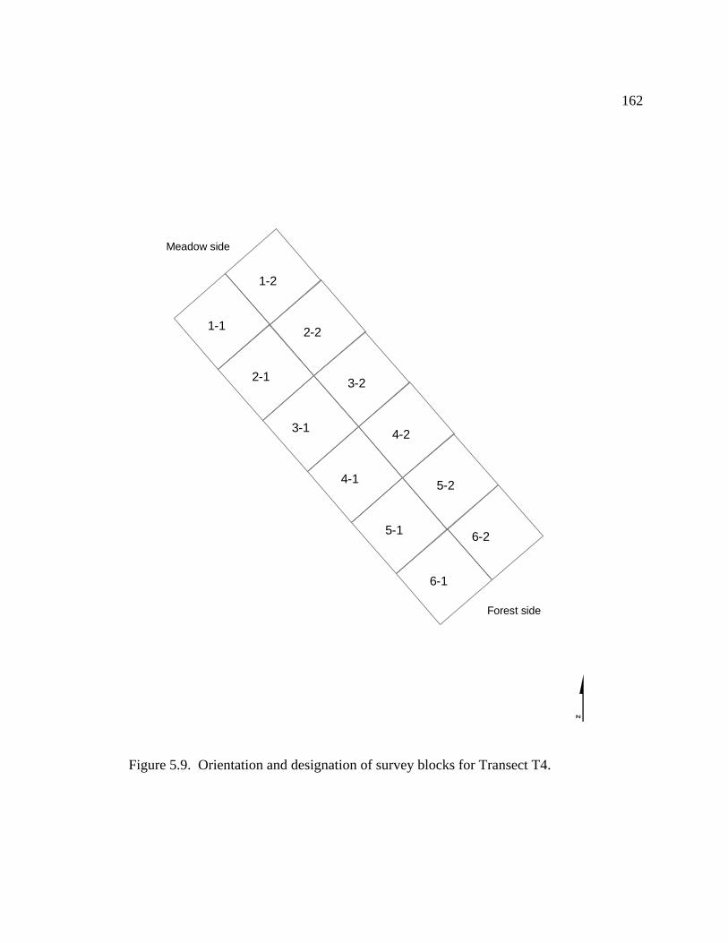
162

1-1

1-2

2-1

2-2

3-1

3-2

4-1

4-2

5-2

6-25-1

6-1

Meadow side

Forest side

Figure 5.9. Orientation and designation of survey blocks for Transect T4.

163

Table 5.6. Transect T4 field data by survey block. Survey Block designation corresponds to Figure 5.9. Species codes are found in Table 5.3. The count column refers to all the occurrences of that species by size class per survey block. The dbh size class pertains to all occurrences and the sample dbh and age pertain to just the subset of trees sampled.

Survey Block Species Count

dbh size class (cm)

Sample dbh (cm)

Age (years)

1-1 Abies grandis 3 seedling X X 1-1 Abies grandis 1 0-5 4.3 32

1-1 Tsuga

heterophylla 2 20-30 22.1 39

1-1 Pseudotsuga

menziesii 1 5-10 8.3 15 1-1 Pinus contorta 2 10-20 15.7 29 1-1 Abies grandis 5 seedling X X

1-1 Pseudotsuga

menziesii 1 0-5 1.7 28

1-1 Tsuga

heterophylla 1 5-10 5.6 21 1-1 Abies grandis 2 0-5 2.4 19 1-1 Pinus contorta 1 20-30 29.2 42 1-2 Abies grandis 4 seedling X X 1-2 Abies grandis 3 0-5 1.8 31

1-2 Pseudotsuga

menziesii 1 10-20 19.2 41 1-2 Pinus contorta 2 10-20 12.8 37 1-2 Abies grandis 2 10-20 13.1 23 2-1 Abies grandis 5 seedling X X

2-1 Tsuga

heterophylla 2 seedling X X 2-1 Abies grandis 1 0-5 1.4 20 2-1 Abies grandis 1 5-10 7.1 17 2-1 Pinus contorta 1 20-30 23.3 X

2-1 Tsuga

heterophylla 3 0-5 2.8 27

2-1 Tsuga

heterophylla 1 5-10 7.2 21

2-2 Pseudotsuga

menziesii 4 10-20 15.4 22

2-2 Tsuga

heterophylla 2 seedling X X

3-1 Pseudotsuga

menziesii 3 5-10 9.9 35

3-1 Pseudotsuga

menziesii 1 0-5 1.2 20 3-1 snag 1 10-20 X X

164

Table 5.6 continued. Transect T4 field data by survey block.

Survey Block Species Count

dbh size class (cm)

Sample dbh (cm)

Age (years)

3-1 snag 1 0-5 X X

3-1 Pseudotsuga

menziesii 2 30-40 38.1 55 3-2 Abies grandis 1 5-10 5.6 27 3-2 snag 1 0-5 X X 3-2 snag 2 10-20 X X

3-2 Tsuga

heterophylla 2 seedling X X 3-2 Abies grandis 1 seedling X X

3-2 Pseudotsuga

menziesii 1 0-5 2.6 28

3-2 Pseudotsuga

menziesii 1 10-20 18.1 39

4-1 Pseudotsuga

menziesii 7 0-5 4.4 25 4-1 Thuja plicata 3 10-20 12.5 35 4-1 snag 1 30-40 X X 4-1 Thuja plicata 1 20-30 26.1 76

4-1 Pseudotsuga

menziesii 4 10-20 8.1 36 4-1 snag 2 10-20 X X 4-1 snag 1 20-30 X X 4-1 snag 1 20-30 X X

4-1 Pseudotsuga

menziesii 1 30-40 36.4 46 4-1 Abies grandis 3 10-20 12.1 25 4-1 Abies grandis 3 5-10 6.7 36 4-1 Abies grandis 1 0-5 1.8 26 4-2 Abies grandis 1 0-5 1.7 21

4-2 Tsuga

heterophylla 3 seedling X

4-2 Pseudotsuga

menziesii 4 5-10 5.9 X

4-2 Pseudotsuga

menziesii 1 20-30 29.7 37

5-1 Pseudotsuga

menziesii 4 0-5 3.8 40

5-1 Pseudotsuga

menziesii 2 seedling X X 5-1 snag 2 5-10 X X 5-1 snag 2 20-30 X X

165

Table 5.6 continued. Transect T4 field data by survey block.

Survey Block Species Count

dbh size class (cm)

Sample dbh (cm)

Age (years)

5-1 Pseudotsuga

menziesii 3 10-20 14.1 31 5-1 Abies grandis 2 0-5 1.5 20 5-1 Abies grandis 2 10-20 19.1 17 5-1 Abies grandis 2 seedling X X

5-1 Tsuga

heterophylla 2 seedling X X

5-1 Pseudotsuga

menziesii 2 seedling X X

5-1 Tsuga

heterophylla 1 0-5 2.7 30 5-1 Abies procera 1 30-40 32.0 44 5-1 Thuja plicata 4 10-20 10.7 57

5-2 Pseudotsuga

menziesii 2 5-10 5.6 42

5-2 Pseudotsuga

menziesii 4 10-20 16.1 37 5-2 Thuja plicata 2 10-20 16.9 43

5-2 Tsuga

heterophylla 1 seedling X X 5-2 Abies grandis 1 seedling X X

5-2 Pseudotsuga

menziesii 2 0-5 2.9 X 6-1 Abies grandis 3 seedling X X

6-1 Tsuga

heterophylla 1 seedling X X

6-1 Tsuga

heterophylla 1 5-10 5.8 43

6-1 Pseudotsuga

menziesii 1 30-40 38.6 83

6-1 Tsuga

heterophylla 1 5-10 7.3 25 6-1 Abies grandis 2 seedling X X

6-1 Tsuga

heterophylla 3 seedling X X

6-1 Tsuga

heterophylla 1 0-5 3.7 33

6-1 Tsuga

heterophylla 1 10-20 14.4 41 6-2 Abies procera 1 5-10 7.1 42

166

Table 5.6 continued. Transect T4 field data by survey block.

Survey Block Species Count

dbh size class (cm)

Sample dbh (cm)

Age (years)

6-2 Tsuga

heterophylla 4 seedling X X 6-2 Abies procera 2 seedling X X

6-2 Pseudotsuga

menziesii 1 20-Oct 13.7 34

6-2 Tsuga

heterophylla 3 10-May 4.6 32 6-2 snag 1 40-50 X X

6-2 Tsuga

heterophylla 2 seedling X X 6-2 Abies grandis 4 seedling X X

6-2 Tsuga

heterophylla 1 10-May 7.9 39

6-2 Pseudotsuga

menziesii 1 70-80 76.5 94 6-2 snag 1 20-30 X X

6-2 Pseudotsuga

menziesii 1 40-50 42.5 66

The species found in this transect include white fir, grand fir, noble fir, lodgepole

pine, Douglas-fir, western hemlock, and western redcedar (Table 5.6). The dominant

species in this transect are grand fir and Douglas-fir. Western hemlock was also

prevalent. Only a handful of lodgepole pine, noble fir, and western redcedar were

present. Sixteen snags of various sizes were counted. The largest and oldest trees

appeared to be the Douglas-fir. Overall, the sizes of the trees increased towards the

southeastern end of the transect (that is, moving toward the forest edge). Lodgepole pine

was only found towards the northwestern end of the transect (i.e., farthest from the forest

edge). Pseudotsuga menziesii occurred throughout the transect but were older the closer

to the transect’s forested end (Figure 5.10). Pinus contorta only occurred 30 meters or

167

more away from the forested end while Thuja plicata did not occur further than 15 meters

from the forested end (Figure 5.10). Abies grandis and Tsuga heterophylla occurred

throughout the transect and did not show a particular relationship between distance for

forested end and age (Figure 5.10). Abies procera occurred only within 10 meters from

the forested end (Figure 5.10).

0

10

20

30

40

50

60

70

80

90

100

0 5 10 15 20 25 30 35

Distance (m) to transect's forest end

Age

(yea

rs)

Abies grandisPinus contortaPseudotsuga menziesiiThuja plicataTsuga heterophyllaAbies procera

Figure 5.10. Age of trees by species in relation to the distance from the forested end of Transect 4.

5.5.2 Comparison of dbh and age

For all Abies grandis samples, there appears to be no relationship between age and

dbh (R2 = 0.04) (Figure 5.11). The same is true when looking at age and dbh in Transect

2 (R2 = 0.002) (Figure 5.12), Transect 3 (R2 = 0.0.18) (Figure 5.13), and Transect 4 (R2 =

0.04) (Figure 5.14). (There was only one Abies grandis in Transect 1.)

168

y = 0.227x + 21.067R2 = 0.0399

0

5

10

15

20

25

30

35

40

45

0 5 10 15 20 25 30

dbh (cm)

Age

(yea

rs)

Figure 5.11. Plot of relationship between age and dbh (cm) for all Abies grandis samples.

y = 0.0583x + 19.89R2 = 0.0021

0

5

10

15

20

25

30

35

0 5 10 15 20 25

dbh (cm)

Age

(yea

rs)

Figure 5.12. Plot of relationship between age and dbh (cm) for Abies grandis samples taken from Transect 2.

169

y = 0.4227x + 22.326R2 = 0.1812

0

5

10

15

20

25

30

35

40

45

0 5 10 15 20 25 30

dbh (cm)

Age

(yea

rs)

Figure 5.13. Plot of relationship between age and dbh (cm) for Abies grandis samples taken from Transect 3. R2 was not calculated due to the small sample size.

y = -0.208x + 25.411R2 = 0.0369

0

5

10

15

20

25

30

35

40

0 5 10 15 20 25

dbh (cm)

Age

(yea

rs)

Figure 5.14. Plot of relationship between age and dbh (cm) for Abies grandis samples taken from Transect 4.

170

For species Pinus contorta in all transects, dbh is only marginally explained by tree

age (R2 = 0.4) (Figure 5.15). When comparing age and dbh in Transects 1 and 3, this

relationship weakens even further (Figures 5.16 and 5.17). There were no Pinus contorta

in Transect 2 and only two in Transect 4.

y = 0.8165x + 12.662R2 = 0.4413

0

5

10

15

20

25

30

35

40

45

0 5 10 15 20 25 30 35

dbh (cm)

Age

(yea

rs)

Figure 5.15. Plot of relationship between age and dbh (cm) for all Pinus contorta samples taken.

171

R2 not calculated due to sample size.

0

5

10

15

20

25

30

0 2 4 6 8 10 12 14

dbh (cm)

Age

(yea

rs)

Figure 5.16. Plot of relationship between age and dbh (cm) for Pinus contorta samples taken in Transect 1. R2 was not calculated due to the small sample size.

y = 0.5331x + 14.859R2 = 0.23210

5

10

15

20

25

30

35

40

45

0 5 10 15 20 25 30

dbh (cm)

Age

(yea

rs)

Figure 5.17. Plot of relationship between age and dbh (cm) for Pinus contorta samples taken in Transect 3.

172

For all Pseudotsuga menziesii sampled, the relationship between age and dbh is

moderately correlated (R2 = 0.6) (Figure 5.18). This relationship becomes stronger in

Transect 3 (Figure 5.19) and Transect 4 (Figure 5.20) where average growth rate is

almost 1 cm dbh per year in both transects. There were no Pseudotsuga menziesii in

Transect 1 and only two in Transect 2.

y = 0.8506x + 21.514R2 = 0.6307

0

10

20

30

40

50

60

70

80

90

100

0 10 20 30 40 50 60 70 80 90

dbh (cm)

Age

(yea

rs)

Figure 5.18. Plot of relationship between age and dbh (cm) for all Pseudotsuga menziesii samples taken.

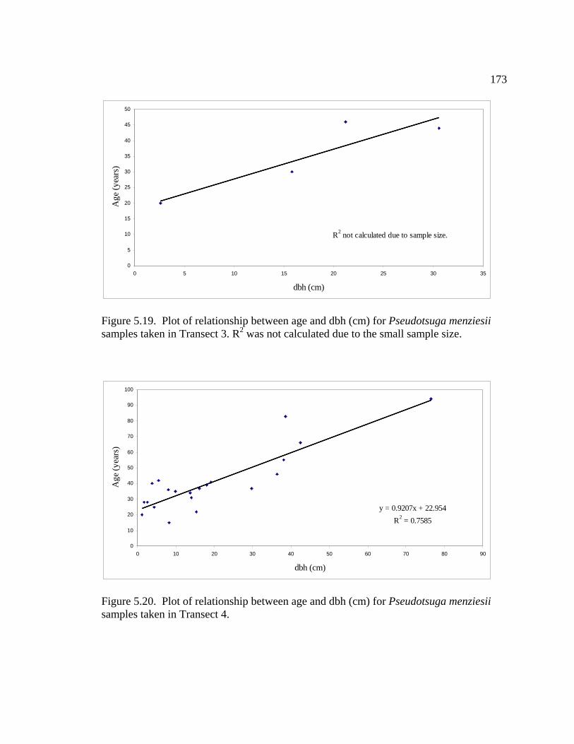
173

R2 not calculated due to sample size.

0

5

10

15

20

25

30

35

40

45

50

0 5 10 15 20 25 30 35

dbh (cm)

Age

(yea

rs)

Figure 5.19. Plot of relationship between age and dbh (cm) for Pseudotsuga menziesii samples taken in Transect 3. R2 was not calculated due to the small sample size.

y = 0.9207x + 22.954R2 = 0.7585

0

10

20

30

40

50

60

70

80

90

100

0 10 20 30 40 50 60 70 80 90

dbh (cm)

Age

(yea

rs)

Figure 5.20. Plot of relationship between age and dbh (cm) for Pseudotsuga menziesii samples taken in Transect 4.

174

The five Thuja plicata sampled in all transects show a moderately strong relationship

between age and dbh (Figure 5.21). No Thuja plicata occurred in Transects 1 or 3. One

occurred in Transect 2 and the remaining 4 occurred in

Transect 4.

R2 not calculated due to sample size.

0

10

20

30

40

50

60

70

80

0 5 10 15 20 25 30

dbh (cm)

Age

(yea

rs)

Figure 5.21. Plot of relationship between age and dbh (cm) for all Thuja plicata samples taken. R2 was not calculated due to the small sample size.

The relationship between age and dbh for all of the Tsuga heterophylla is

Very weak (R2 = 0.1) (Figure 5.22). However, this relationship appears quite strong

when looking only at data collected in Transect 3 (Figure 5.23) with an average growth

rate of 0.4 cm dbh per year. The relationship is weak in Transect 4 (R2 = 0.2) (Figure

5.24). There are no Tsuga heterophylla in Transect 1 and only one in Transect 2.

175

y = 0.4167x + 24.851R2 = 0.1054

0

5

10

15

20

25

30

35

40

45

50

0 5 10 15 20 25 30

dbh (cm)

Age

(yea

rs)

Figure 5.22. Plot of relationship between age and dbh (cm) for all Tsuga heterophylla samples taken.

R2 not calculated due to sample size.

0

5

10

15

20

25

30

0 5 10 15 20 25 30

dbh (cm)

Age

(yea

rs)

Figure 5.23. Plot of relationship between age and dbh (cm) for Tsuga heterophylla samples taken in Transect 3. R2 was not calculated due to the small sample size.

176

y = 0.6067x + 27.27R2 = 0.1988

0

5

10

15

20

25

30

35

40

45

50

0 5 10 15 20 25

dbh (cm)

Age

(yea

rs)

Figure 5.24. Plot of relationship between age and dbh (cm) for Tsuga heterophylla samples taken in Transect 4.

5.5.3 Snag size in Transect 4 relative to forest edge

Only two Transects (T1: Burnt Island and T4: Green Edge) contained snags. The

snags in T1 were 10-80 cm dbh (Table 5.2) and had burned in 1996. There is no way of

knowing if they died previous to or because of the fire. The snags in T4 were 0-50 cm

dbh (Table 5.6) and were not burned indicating they may have died from stem exclusion

or disease. There is a slight pattern of the larger snags occurring closer to the forested

end of Transect 4 (Figure 5.25).

177

0

5

10

15

20

25

30

35

40

45

50

0 5 10 15 20 25

Distance (m) to transect's forested end

Med

ian

valu

e of

dbh

siz

e cl

ass

(cm

)

Figure 5.25. Plot of relationship between snag size and distance from forested end of Transect 4.

5.5.4 Relationship between seedling occurrence and location in transect

In Transect 1, Abies concolor and Abies grandis seedlings occur throughout most of

the transect except in the survey block closest to the forest edge (Figure 5.26). Pinus

contorta seedlings only occur in the survey blocks at least 20 meters from the end of the

transect that is closest to the forest edge (Figure 5.26).

178

0

5

10

15

20

25

30

35

40

45D

ista

nce

(m) f

rom

end

of t

rans

ect

with

line

of t

rees

Abies concolorAbies grandisPinus contorta

Figure 5.26 Plot of relationship between seedling occurrence and distance to end of Transect 1 closest to forest edge.

In transect 2, Abies grandis seedlings occurs throughout the transect while Abies

concolor, and Thuja plicata seedlings occur closer to the upslope end of the transect

(Figure 5.27). Pseudotsuga menziesii seedlings occur in the approximate middle of the

transect (Figure 5.27).

179

0

5

10

15

20

25D

ista

nce

(m) f

rom

do

wns

lope

end

of t

rans

ect

Abies concolor

Abies grandis

Anies grandisor concolorPseudotsugamenziesiiThuja plicata

Figure 5.27 Plot of relationship between seedling occurrence and distance to downslope end of Transect 2.

Pinus contorta are the only seedlings counted in Transect 3 and occur more often the

further from the forested end of the transect (Figure 5.28).

180

0

5

10

15

20

25

30

35D

ista

nce

(m) t

o tra

nsec

t end

cl

oses

t to

fore

st e

dge

Pinus contorta

Figure 5.28 Plot of relationship between seedling occurrence and distance to forested end of Transect 3.

In Transect 4, Abies grandis and Tsuga heterophylla seedlings occur throughout out

the transect though Tsuga heterophylla does not occur in the survey block closest to the

meadow edge (Figure 5.29). Abies procera and Pseudotsuga menziesii seedlings occur

within 10 meters of the forested end of the transect (Figure 5.29).

181

0

5

10

15

20

25

30

35D

ista

nce

(m) t

o tra

nsec

t's fo

rest

ed e

nd Abies grandisAbies proceraPseudotsuga menziesiiTsuga heterophylla

Figure 5.29 Plot of relationship between seedling occurrence and distance to forested end of Transect 4.

5.6 Discussion

The survey provides a pattern of species establishment and dominance. Though not

every tree was sampled, there were obvious trends in the transects that could be

understood through each species’ tolerances to fire and shade. Site characteristics and

land management also provide clues to invasion timing and patterns.

The T1 and T3 Transects were burned in 1996 and both contain a large number of

Pinus contorta seedlings that are not found in T2 or as prevalent in T4. Though Burns

and Honkala (1990) state that serotinous cones are not prevalent in Oregon, this large

number of seedlings may indicate this is a case where they do occur and the previous

management caused this species to proliferate. The mineralization of the soil in this area

from the prescribed burn may have been good seed bed preparation, contributing to the

182

large number of seedlings established after the fire. Future management should consider

the intensity required to eradicate specific species under various age and density

conditions and balance it with the undesirable impacts of such an intensity (i.e. soil

mineralization promotes seedling establishment). In the case of Transects 1 and 3,

continued tree removal or burning needs to occur to remove post-fire invasion of Pinus

contorta.

Transects 3 and 4 are “edge” transects where invasion occurs from the historic forest

edge. Similar to what Jakubos and Romme (1993) observed in their study area, overall

trees became younger the further they were form the forested end of the transect.

However, when looking at just Abies grandis and Tsuga heterophylla in Transect 4

(Figure 5.10), the ages appear to be roughly the same suggesting seedlings established all

at once in a band similar to what Lepofsky (2003) found. If seedlings are establishing

progressively, it may be because with each new seedling, the soil conditions and

microclimate are becoming more favorable for subsequent seedling establishment.

Establishment all at once in a band may indicate the ameliorating effects of the

previously established trees have a certain range of influence reflected by the band’s

width. In either case, this indicates eradication of the early invaders may tide the flow of

subsequent invaders. Transect 3, the burnt island, doesn’t have a forested end but one

end is closer to the forest than the other and the Pinus contorta show a linear decrease in

age with distance to forest relationship. Transect 4 reflects an invasion pattern similar to

183

the “leap and fill” patterns described by Norman and Taylor (2005) and Franklin et al.

(1971).

The T2 encroachment pattern may be explained by the ameliorating effects of

established trees and potential reduced snow pack (Lepofsky et al., 2003). The largest

and presumably oldest tree, an 80-90 cm dbh Abies grandis or Abies concolor (or a cross

between the two), was too large to core with available equipment. The surrounding trees

were mostly between 25-30 years old and significantly smaller in girth. The single large

tree may have provided favorable conditions for the younger trees to establish. The

relatively uniform age of most of the non-seedlings may also indicate that reduced

snowpack since 1970 (as suggested by Lepofsky et al. (2003)) on the steep south facing

slope allowed for a greater growing season and encouraged conifer germination. This

area was also heavily grazed and the cessation of grazing may be a contributing factor to

invasion.

The burnt edge, T3, occurs at the margin of a dry meadow community (Salix, 2005).

Shade from the older (30-46 years) Douglas-fir that occurs on the forested end of the

transect may have facilitated establishment of shade tolerant western redcedar and

western hemlock. The presence of western hemlock aged 17-27 years indicates that the

prescribed fire of 1996 probably was of very low intensity. The co-dominance of grand

fir with lodgepole pine may be a reflection of the moderate fire resistance of grand fir or

its ability to tolerate more sun than the western hemlock or western redcedar.

184

Transect T4, the green edge, is within the mesic meadow community identified by

Salix (2005). It is most shaded of all the transects and terminates at a creek. Lodgepole

pine occurs only at the meadow end of the transect, suggesting that heavy shade further

precludes its establishment there. Grand fir and Douglas-fir dominate, shading their even

more shade tolerant associate western hemlock. Perhaps the small amount of western

redcedar present is due to heavy browsing by deer and elk. There were many scat signs

and game trails in this area. This transect was unique in that it had many small diameter

snags with no evidence of char so presumably not killed by fire. These small snags may

have been killed during the stem exclusion phase of this forest’s establishment.

The pattern of encroachment in T4 reflects an upslope creep from forested to

previously open areas. The ages of the trees become younger as the meadow edge is

approached. Even more so than the green island, a pattern of “leap and fill” can be found

in this area: the meadow side of this transect is being encroached from all sides and is

nearly gone. Like all the other transects, this is a steep, south facing slope that was once

heavily grazed by sheep. Therefore, increased wet periods between 1945 and 1985

(Miller and Halpern, 1998) and grazing may also be responsible for the timing of

invasion in this transect.

Generally certain expected patterns were found. Shade intolerant Pinus contorta

occurred in open areas and edges and shade tolerant Thuja plicata and Tsuga

heterophylla occurred closer to the shaded forested end of transects. The latter were not

185

found in areas that had burned owing to their fire intolerance. The distribution of

seedlings demonstrated no patterns but the sample size was too small to consider this

significant.

Though a subset of trees were destructively sampled and their age determined by

counting rings, strong correlation between age and dbh could be made only for

Pseudotsuga menziesii. This suggests that for future fine-scale encroachment studies that

intend to relate specific fire, climate, or land use events to encroachment, all trees should

be aged for best results.

186

6. Conclusion

This purpose of this study was to determine the distribution of meadows within the

Willamette National Forest, identify conifer encroachment patterns into meadows within

the Chucksney-Grasshopper meadow complex, and understand fine scale encroachment

in one meadow. Three methods of analysis at three scales were used to achieve this:

satellite remote sensing, historic photographic interpretation, and field surveys. The

context of this study is the increased management and restoration of meadow habitat by

agencies, such as the US Forest Service, in light of the decrease of its areal extent.

A land cover classification dataset was created that identifies meadow cover in the

Willamette National Forest. It fills the data gap created by the previous focus of forest

management on timber resources. The meadow classification was combined with data

derived from digital elevation models to characterize the distribution of meadows in the

western and high Cascades of Oregon. In the western Cascades, meadows are

concentrated on steep, south and east facing ridges between 1000 and 2000m in

elevation. In the high Cascades, meadows are concentrated in valleys between 500 and

1000 meters in elevation and occur on both gentle and steep east and south facing slopes.

Historic photographic interpretation in combination with GIS analysis revealed

different encroachment pattern in the Chucksney-Grasshopper complex. All meadows

demonstrated encroachment occurred closer to existing trees than further from them.

Encroachment was significant on steep, south and east facing slopes in some meadows,

187

but also on gentle, west facing slopes in other meadows. Vegetation cover, land use

history, and fire history, and climate effects may be factors in these differing patterns.

This preliminary analysis lays the groundwork for a potential invasion risk tool. The

multiple factors affecting invasion that were analyzed or identified can be combined with

invasion patterns to create a risk model that can be used by land managers to assess and

prioritize maintenance and restoration activities.

The results of the field sampling and analysis of meadow 4 in the Chucksney-

Grasshopper complex provide insight to how invasion occurs at a fine scale and

potentially how to thwart it. It appears as though the prescribed burns conducted in 1996

promoted Pinus contorta invasion suggesting a review and revision of current burning

methods. Management methods may also be revised based on encroachment patterns

found in the field transects. Whether seedlings establish all at once in a band or

progressively from older trees or forest edges, they facilitate the subsequent

establishment of other seedlings suggesting early eradication prevents increased rates of

invasion.

This study provides some guidance to managers but a large body of work by

multidisciplinary researchers provides a greater context for management. If the purpose

of management is to mitigate conifer invasion into meadows, then the drivers of invasion

must be considered. Three dominant drivers are grazing practices, changes in fire

regime, and climate changes. The impact of grazing cessation in the 1960s has occurred

188

and is likely irreversible. The effect of tree establishment on soil conditions and the

transient nature of meadow species in the seed bank prevents meadow species from re-

establishing (Haugo and Halpern, 2007; Lang and Halpern, 2007). Meadows in the WNF

may have been artificially maintained through fire by Native Americans until the mid-

19th century (Boyd, 1999; French, 1999; Robbins, 1999; Whitlock, 2004, Lepofsky,

2003) and natural fire regimes have been altered by subsequent land management or

through climate change (Westerling, et al., 2006). Regardless of the cause of the changes

in fire regimes, fire has a role in the maintenance of meadows. Researchers Swanson,

Cissel, and Halpern, among others, are involved in on-going studies that look at the

effects of alternative fire management strategies on soil and vegetation. Lessons learned

from these studies will enable managers to determine the severity and frequency of fires

needed to maintain or restore meadow habitat without promoting the establishment of fire

adapted tree species such as Pinus contorta or fire adapted ruderals that will outcompete

native meadow vegetation. Finally, climate change has an impact on meadows in

multiple ways. On steep dry slopes, increased precipitation can favor conifer seedling

establishment while on cold north slopes, increased temperatures can reduce snowpack

and lengthen the growing season facilitating conifer invasion (Miller and Halpern, 1998).

Increased temperatures have also resulted in drought conditions which have been

correlated to more frequent and longer lasting wildfires in the western US (Westerling et

al., 2006). This change in fire regime may impact meadows by mineralizing soils for

conifer seedling establishment and destroying meadow species’ seed banks. The role of

managers is to understand what drivers are impacting particular meadow habitat and

189

develop maintenance and restoration strategies accordingly. Managers should also

consider that meadows and forests have formed a shifting mosaic since the mid-Holocene

(Jakubos and Romme, 1993) and that some drivers of invasion, such as climate change,

cannot be mitigated.

190

Literature Cited Agee, J.K., 1993. Fire ecology of Pacific Northwest Forests, Island press.

Washington, D.C. Boardman, J. W., Kruse, F. A., and Green, R. O., 1995, Mapping target signatures

via partial unmixing of AVIRIS data: in Summaries, Fifth JPL Airborne Earth Science Workshop, JPL Publication 95-1, v. 1, pp. 23-26.

Boyd, R., 1999. Introduction and Strategies of Indian Burning in the Willamette

Valley in Indians, Fire, and the Land in the Pacific Northwest. R. Boyd ed. Oregon State University Press, Corvallis, Oregon.

Burke, C.J., 1980. Historic fires in the central Western Cascades, Oregon. Thesis,

Oregon State University, Corvallis, Oregon. Burns, R.M., and B.H. Honkala, 1990. Silvics of North America: 1. Conifers; 2.

Hardwoods. USDA FS Agriculture Handbook 654. U.S. Department of Agriculture, Forest Service, Washington, DC. vol.2, 877 p.

Cohen, W.B., T.A. Spies, T.K. Maiersperger, and D.R. Oetter – GIS, 1988. Land

Cover of Western Oregon raster format data. Obtained from LARSE January 2007 (http://www.fsl.orst.edu/larse/wov/88wov.html).

Cohen, W.B., M. Fiorella, J. Gray, E. Helmer, and K. Anderson, 1998. The

efficient and accurate method for mapping forest clear cuts in the Pacific Northwest using Landsat imagery. Photogrammetric engineering and remote sensing, v. 64, no. 4, p. 293-300.

Cohen, W.B., T.A. Spies, and M. Fiorella, 1995. Estimating the age and structure of forests in a multi-ownership landscape of western Oregon, U.S.A. International Journal of Remote Sensing, v. 16, no. 4: 721-746.

Cohen, W.B., T.A. Spies, R.J. Alig, D.R. Oetter, T.K. Maiersperger, and M.

Fiorella, 2002. Characterizing 23 Years (1972-1995) of Stand Replacement Disturbance in Western Oregon Forests with Landsat Imagery. Ecosystems 5: 122-137.

Cohen, W.B. and S. Lennartz - GIS, 2004. 1972-2004 Western Oregon Stand

Replacement Disturbance Map. ESRI GRID format. Oregon. http://www.fsl.orst.edu/larse/

191

Coop, J.D. and T.J. Givnish, 2007. Spatial and temporal patterns of recent forest encroachment in montane grasslands of the Valles Caldera, New Mexico, USA. Journal of Biogeography, v. 34: 914-927.

Coops, N, P. Ryan, A. Loughhead, B. Mackey, J. Gallant, I. Mullen, and M.

Austin, 1998. Developing and Testing Procedures to Predict Topographic Position from Digital Elevation Models (DEM) for Species Mapping (Phase I). CSIRO Forestry and Forest Products: Client Report No: 271, http://www.ffp.csiro.au/nfm/mdp/topo/topo_home.htm (Accessed May 2007.)

Courtney, S.P., J.A. Blakesley, R.E. Bigley, J.P. Dumbacher, R.C. Fleisher, A.B.

Franklin, J.F. Franklin, R.J. Gutierrez, J.M. Marzluff, L. Sztukowksi, 2004. Scientific evaluation of the status of the Northern Spotted Owl. Sustainable Ecosystems Institute, Portland, Oregon. http://www.sei.org/owl/finalreport/finalreport.htm

Crippen, R.E., 1988. The dangers of underestimating the importance of data

adjustments in band ratioing. International Journal of Remote Sensing, v. 9, no. 4, p. 767-776.

Debinksi, D.M. M.E. Jakubauskas, and K.Kindscher, 2000. Environmental

Monitoring and Assessment, 64: 213-225. Dunwiddie, P.W., 1977. Recent tree invasion of subalpine meadows in the wind

river mountains, Wyoming, Arctic and Alpine Research, v 9, no. 4, p393-399. ENVI, v. 4.2. Help Documentation. Evans, R.D. and R.W. Fonda, 1990. The influence of snow on subalpine meadow

community pattern, North Cascades, Washington. Canadian Journal of Botany, v. 68.

Ford, P., J. Kertis, J. Philips, R. Seitz, S. Swetland, and J. Cisel, 1998. Chucksney

Mountain Meadow Restoration, USFS report, dated March 10, 1998. Unpublished.

Franklin, J.F. W.H. Moir, G.W. Douglas, and C. Wiberg, 1971. Invasion of

subalpine meadows by trees in the Cascade Range, Washington and Oregon. Arctic and Alpine Research, v. 3, no. 3: 215-224.

Franklin, J.F. and C.T. Dyrness, 1988. Natural vegetation of Oregon and

Washington. Corvallis, OR: Oregon State University Press.

192

French, D., 1999. Aboriginal Control of Huckleberry Yield in Indians, Fire, and the Land in the Pacific Northwest. R. Boyd ed. Oregon State University Press, Corvallis, Oregon.

Hadjimitsis, D.G., C.R.I. Clayton, and V.S. Hope, 2004. An assessment of the

effectiveness of atmospheric correction algorithms through the remote sensing of some reservoirs. International Journal of Remote Sensing, v. 25, no. 18, p. 3651-3674.

Haugo, R.D. and C.B. Halpern, 2007. Vegetation responses to conifer

encroachment in a western Cascade meadow: a chronosequence approach. Canadian Journal of Botany, v. 85: 285-298.

Herzfeld, U.C. and C.A. Higginson, 1996. Automated geostatistical seafloor classification – Principles, parameters, feature vectors, and discrimination criteria. Computers & Geosciences, v. 22, no.1: 35-52. Idaho Forest Products Commission. http://www.idahoforests.org/ (Accessed

March, 2007) Jakubos, B. and W.H. Romme, 1993. Invasion of Subalpine Meadows by

Lodgepole Pine in Yellowstone National Park, Wyoming, U.S.A. Arctic and Alpine Research, v 25, no. 4, p 382-390.

Jensen, J.R., 2005. Introductory Digital Imaging Processing, A remote Sensing

Perspective, third edition. Pearson Prentice Hall, Upper Saddle River, New Jersey.

Jensen, E.C. and C.R. Ross, 2005. Trees to Know in Oregon. Oregon State

University Extension Service, Corvallis, Oregon. Jones, J.A., and G.E. Grant, 1996. Peak flow responses to clear-cutting and roads

in small and large basins, western Cascades, Oregon. Water Resources Research, v. 32, no. 4: 959-974.

Jones, J.A., 2007. Personal communication, July, 2007. Laboratory for Applications in Remote Sensing in Ecology (LARSE).

http://www.fsl.orst.edu/larse/ (Accessed October, 2006.) Lang, N.L. and C.B. Halpern, 2007. The soil seed bank of a montane meadow:

consequences of conifer encroachment and implications for restoration. Canadian Journal of Botany, v. 85: 557-569.

193

Lennartz, S., 2005. Oregon Land Change Mapping. Conference paper: Pecora 16 “Global Priorities in Land Remote Sensing”, October 23-27, 2005, Sioux Falls, South Dakota.

Lepofsky, D., E.K. Heyerdahl, K. Lertzman, D. Schaepe, and B. Mierendorf, 2003.

Historical meadow dynamics in southwest British Columbia: a multidisciplinary analysis. Conservation Ecology, v 7(3): 5.

Nolin, A., 2007. Personal communication, May 2007. Norman, S.P. and A.H. Taylor, 2005. Pine forest expansion along a forest-

meadow ecotone in northeastern California, USA. Forest Ecology and Management, 215: 51-68.

Norton, H.H., R. Boyd, and W. Hunn, 1999. The Klikitat Trail of South-central

Washington in Indians, Fire, and the Land in the Pacific Northwest. R. Boyd ed. Oregon State University Press, Corvallis, Oregon.

Matarrese, M. 1992. Maintenance of Seral Meadow Ecosystems in the Chucksney

Mountain Roadless Area, a unpublished paper presented for completion of requirements for Technical Fire Management, Willamette National Forest.

McKnight, T.L., 1999. Physical Geography, A Landscape Appreciation, Sixth

Edition. Upper Saddle River, NJ: Prentice Hall.

Oregon Geospatial Enterprise Office - GIS, 2001. http://gis.oregon.gov/DAS/EISPD/GEO/sdlibrary.shtml River Reach data. (Accessed March, 2007.)

Orr, W.N. and E.L. Orr. 2002. Geology of the Pacific Northwest, Second Edition.

New York, NY: McGraw Hill p.73-112.

Miller, E.A. and C.B. Halpern, 1998. Effects of environment and grazing disturbance on tree establishment in meadows of the central Cascade Range, Oregon, USA. Journal of Vegetation Science, v. 9: 265-282.

Oregon Department of Fish and Wildlife (ODFW), 2006. Oregon Conservation

Strategy. http://www.dfw.state.or.us/conservationstrategy/document_pdf/b-eco_wc.pdf (Accessed March, 2007.)

PRISM Group - GIS, Oregon State University, 2004. http://www.prismclimate.org

(Accessed May, 2007.)

194

Rakestraw, L. and M. Rakestraw, 1991. History of the Willamette National Forest. USDA Forest Service, Willamette National Forest, Eugene Oregon.

Robbins, W.G., 1999. Landscape and Environment in Indians, Fire, and the Land

in the Pacific Northwest. R. Boyd ed. Oregon State University Press, Corvallis, Oregon.

Salix Associates, 2005. Grasshopper Mountain to Chucksney Mountain: 8- Meadow Plant and Wildlife Inventory and Mapping Project. Report for the Willamette National Forest.

Seitz, R., A. Martinez, 2003. Grasshopper/Chucksney Meadow Complex Field

Reconnaissance USFS report dated September 2, 2003. Unpublished. Strahler, A. and A. Strahler, 2002. Physical Geography – Science and Systems of

the Human Environment, second edition. John Wiley & Sons, Inc., New York, NY.

Takaoka, S. and F.J. Swanson, 2006. Change in extent of meadows and shrub

fields in the central western Cascade Range, Oregon, U.S.A. Publish pending.

Taylor, A.H., 1990. Tree invasion in meadows of Lassen Volcanic National Park,

California, Professional Geographer, 42(4), p 457-470. Taylor, A.H., 2000. Fire regimes and forest changes in mid and upper montane

forests of the southern Cascades, Lasses Volcanic National Park, California, U.S.A. Journal of Biogeography, v. 27, no. 1, p 87-104.

Thompson, J., 2007. Mountain meadows – Here today, gone tomorrow? Meadow

science and restoration. Science Findings, USDA Pacific Northwest Research Station, Portland, OR USA.

USFS, 1964. District Ranger Memo: Chucksney Mt. Allotment (Lodgepole Pine

Eradication Project) Dated November 17, 1964. USFS, 1981. Chucksney Mountain Undeveloped Roadless Recreation Area

Management Plan, unpublished. USDA Forest Service. Ecological Subregions of the United States. Chapter 25,

Section M242B, Western Cascades. http://www.fs.fed.us/land/pubs/ecoregions/ch25.html#M242B (Accessed March 2007.)

195

USDA Natural Resources Conservation Service, 2006. Keys to Soil Taxonomy, 10th edition.

Vale, T.R., 1981. Tree Invasion of Montane Meadows in Oregon. American

Midland Naturalist, v. 105, no. 1: 61-69. van der Meer, F. and S.M. de Jong, 2000. Improving the results of spectral

unmixing of Landsat Thematic Mapper imagery by enhancing the orthogonality of end-members. International Journal of Remote Sensing, v. 21, no. 15, p. 2781-2797.

Wearne, L.J. and J.W. Morgan, 2001. Recent forest encroachment into subalpine

grasslands near Mount Hotham, Victoria, Australia. Arctic, Antarctic, and Alpine Research, v. 33, no. 3: 369-377.

Westerling, A.L., H.G. Hidalgo, D.R. Cayan, and T.W. Swetnam, 2006. Warming and earlier spring increase western US forest wildfire activity. Science, v. 313. Whitlock, C., 2004. Land management: Forests, fires and climate. Nature,

432:28-29. Willamette National Forest. Home.

http://www.fs.fed.us/r6/willamette/forest/facts/index.html (Accessed March 2007.)

Willamette National Forest - GIS, 1991.

http://www.fs.fed.us/r6/willamette/manage/gis/ GEOL layer last updated June 2006. (Accessed March 2007.)

Willamette National Forest - GIS, 2006.

SHABS layer obtained by request from Willamette National forest October, 2006. Willamette National Forest - GIS, 1992.

http://www.fs.fed.us/r6/willamette/manage/gis/ SRI layer last updated 1992. (Accessed March 2007.)

Willamette National Forest, 2006. Decision Memo: Chucksney & Grasshopper

Meadow Restoration. McKenzie River and Middle Fork Ranger Districts, Willamette national Forest.

Williams, G.W., 2006. The Forest Service: Fighting for Public Lands.

Greenwood Press, Westport, CT.

196

Woods, A., S. Bryce, and J. Omernik, 2003. Level III and IV Ecoregions of Oregon. GIS Data: USEPA http://www.epa.gov/wed/pages/ecoregions.htm (Accessed May, 2007.)

Zimmerman, N. 2000. Topographic Position Mapping Routines.

http://www.wsl.ch/staff/niklaus.zimmermann/programs/aml4_2.html (Accessed March 2007.)