jpo_2003_4

APRIL 2003 863J A N S S E N

q 2003 American Meteorological Society

Nonlinear Four-Wave Interactions and Freak Waves

PETER A. E. M. JANSSEN

ECMWF, Shinfield Park, Reading, United Kingdom

(Manuscript received 30 April 2002, in final form 11 October 2002)

ABSTRACT

Four-wave interactions are shown to play an important role in the evolution of the spectrum of surface gravitywaves. This fact follows from direct simulations of an ensemble of ocean waves using the Zakharov equation.The theory of homogeneous four-wave interactions, extended to include effects of nonresonant transfer, comparesfavorably with the ensemble-averaged results of the Monte Carlo simulations. In particular, there is good agree-ment regarding spectral shape. Also, the kurtosis of the surface elevation probability distribution is determinedwell by theory even for waves with a narrow spectrum and large steepness. These extreme conditions arefavorable for the occurrence of freak waves.

1. Introduction

At present there is a considerable interest in under-standing the occurrence of freak waves. The notion offreak waves was first introduced by Draper (1965), andthis term is applied for single waves that are extremelyunlikely as judged by the Rayleigh distribution of waveheights (Dean 1990). In practice this means that whenone studies wave records of a finite length (say of 10–20 min), a wave is considered to be a freak wave if thewave height H (defined as the distance from crest totrough) exceeds the significant wave height HS by afactor 2.2. It is difficult to collect hard evidence on suchextreme wave phenomena because they occur so rarely.Nevertheless, observational evidence from time seriescollected over the past decade does suggest that for largesurface elevations the probability distribution for thesurface elevation deviates substantially from the one thatfollows from linear theory with random phase, namelythe Gaussian distribution (e.g., Wolfram and Linfoot2000).

There are a number of reasons why freak wave phe-nomena may occur. Often, extreme wave events can beexplained by the presence of ocean currents or bottomtopography that may cause wave energy to focus in asmall area because of refraction, reflection, and wavetrapping. These mechanisms are well understood andmay be explained by linear wave theory (e.g., Lavrenov1998).

Trulsen and Dysthe (1997) argue, however, that it isnot well understood why exceptionally large waves may

Corresponding author address: Peter A. E. M. Janssen, EuropeanCentre for Medium-Range Weather Forecasts, Shinfield Park, Read-ing RG2 9AX, United Kingdom.E-mail: [email protected]

occur in the open ocean away from nonuniform currentsor bathymetry. As an example they discuss the case ofan extreme wave event that happened on 1 January 1995in the Norwegian sector of the North Sea. Their basicpremise is that these waves can be produced by non-linear self modulation of a slowly varying wave train.An example of nonlinear modulation or focusing is theinstability of a uniform narrowband wave train to side-band perturbations. This instability—known as the side-band, modulational, or Benjamin–Feir instability (Ben-jamin and Feir 1967)—will result in focusing of waveenergy in space and/or time as is illustrated by the ex-periments of Lake et al. (1977).

To a first approximation, the evolution in time of theenvelope of a narrowband wave train is described bythe nonlinear Schrodinger equation. This equation,which occurs in many branches of physics, was firstdiscussed in the general context of nonlinear dispersivewaves by Benney and Newell (1967) (see also Ostrows-kii 1967). For water waves it was first derived by Zak-harov (1968) using a spectral method and by Hasimotoand Ono (1972) and Davey (1972) using multiple-scalemethods. The nonlinear Schrodinger equation in one-space dimension may be solved by means of the inversescattering transform. For vanishing boundary condi-tions, Zakharov and Shabat (1972) found that for largetimes the solution consists of a combination of envelopesolitons and radiation modes, in analogy with the so-lution of the Korteweg–de Vries equation. However, fortwo-dimensional propagation, Zakharov and Rubenchik(1974) discovered that envelope solitons are unstable totransverse perturbations, and Cohen et al. (1976) foundthat a random wave field would break up envelope sol-itons. This meant that solitons could not be used as

864 VOLUME 33J O U R N A L O F P H Y S I C A L O C E A N O G R A P H Y

building blocks of the nonlinear evolution of gravitywaves.

For periodic boundary conditions, the solution of thenonlinear Schrodinger equation is more complex. Lin-ear stability analysis of a uniform wave train showsthat close side bands grow exponentially in time ingood qualitative agreement with the experimental re-sults of Benjamin and Feir (1967) and Lake et al.(1977). For large times there is a considerable energytransfer from the carrier wave to the side bands. Inone-space dimension (1D) if there is only one unstableside band, Fermi–Pasta–Ulam recurrence occurs (Yuenand Ferguson 1978) in qualitative agreement with theexperiments of Lake et al. (1977). In the presence ofmany unstable side bands, the evolution of a narrow-band wave train becomes much more complex. No re-currence is then found (Caponi et al. 1982), and theseauthors have termed this confined chaos in a nonlinearwave system because most of the energy resides in theunstable modes. Also, in two-space dimensions (2D)the phenomenon of recurrence is the exception ratherthan the rule. In addition, in 2D the instability regionis unbounded in the perturbation wave vector space,resulting in energy leakage to high wave-numbermodes; hence there is no confined chaos in 2D (Martinand Yuen 1980). This suggests that the 2D nonlinearSchrodinger equation is inadequate to describe the evo-lution of weakly nonlinear waves. This was pointedout already by Longuet-Higgins (1978) who performeda stability analysis on the exact equations and foundthat the instability region is finite in extent. More-re-alistic evolution equations such as the fourth-orderevolution equation of Dysthe (1979) or the Zakharovequation (1968) are needed to give an appropriate de-scription of nonlinear gravity waves in two-space di-mensions.

Nevertheless, studies of the properties of the non-linear Schrodinger equation have been vital in un-derstanding the conditions under which freak wavesmay occur. This was discussed in detail by Osborneet al. (2000). For periodic boundary conditions, theone-dimensional nonlinear Schrodinger equation maybe solved by the inverse scattering method as well.The role of the solitons is then replaced by unstablemodes. In the linear regime, these modes just describethe evolution in time according to the Benjamin–Feirinstability, whereas, by means of the inverse scatter-ing transform, the fate of the unstable mode may befollowed right into the nonlinear regime. Using theinverse scattering transform, the solution of the 1Dnonlinear Schrodinger equation may be written as a‘‘linear’’ superposition of stable modes, unstablemodes, and their mutual nonlinear interactions. Here,the stable modes form a Gaussian background wavefield from which the unstable modes occasionally riseup and subsequently disappear again, repeating theprocess quasi-periodically in time. Making use of theinverse scattering transform, these authors readily

construct a few examples of giant waves from the one-dimensional nonlinear Schrodinger equation. Thequestion now is what happens in the case of two-dimensional propagation. The notion of solitons is nolonger useful, because solitons are unstable in twodimensions. Osborne et al. (2000) show that unstablemodes do indeed still exist and that in the nonlinearregime they can take the form of large-amplitudefreak waves. Furthermore, the notion of unstablemodes seems to be a generic property of deep-waterwave trains as the authors find nonlinear unstablemodes in both the one- and two-dimensional versionsof Dysthe’s fourth-order evolution equation. To sum-marize this discussion, it seems that freak waves arelikely to occur as long as the wave train is subject tononlinear focusing. In addition, we only need to studythe case of one-dimensional propagation, because itcaptures the essentials of the generation of freakwaves.

Therefore, in the context of the deterministic ap-proach to wave evolution, there seems to be a reasonabletheoretical understanding of why in the open ocean freakwaves occur. In ocean wave forecasting practice onefollows, however, a stochastic approach; that is, oneattempts to predict the ensemble average of a spectrumof random waves because knowledge on the phases isnot available. The main problem then is to what extentone can make statements regarding the occurrence offreak waves in a random wave field. Of course, in thecontext of wave forecasting only statements of a prob-ablistic nature can be made. Because freak waves implyconsiderable deviations from the normal Gaussian prob-ability distribution function (pdf ) of the surface ele-vation, the main question therefore is whether one candetermine in a reliable manner the pdf of the surfaceelevation. Because the wave spectrum plays a centralrole in the stochastic approach, the question thereforeis whether for given wave spectrum the probability ofextreme events may be determined.

Present-day wave forecasting systems are based onthe energy balance equation (Komen et al. 1994), in-cluding a parameterized version of Hasselmann’s four-wave nonlinear transfer (Hasselmann 1962). Resonantfour-wave interactions for a random, homogeneous seaplay an important role in the evolution of the spectrumof wind waves, because on the one hand they determinethe high-frequency part of the spectrum, giving rise toan v24 tail (Zakharov and Filonenko 1968) while onthe other hand the peak of the spectrum is shifted towardlower frequencies. The homogeneous nonlinear inter-actions give rise to deviations from the Gaussian pdffor the surface elevation, because the third-order non-linearity generates fourth cumulants of the pdf while thefinite fourth cumulant results in spectral change. Animportant issue is, however, whether the standard ho-mogeneous theory can properly describe the generationof freak waves, simply because it does not seem toincorporate the Benjamin–Feir instability mechanism


(Alber 1978; Alber and Saffman 1978; Crawford et al.1980; Janssen 1983b). This follows from simple scalingconsiderations applied to the Hasselmann evolutionequation for four-wave interactions. Because the rate ofchange of the action density N is proportional to N 3,the nonlinear transfer occurs on the time scale TNL 5O(1/e4v0). Here, e is a typical wave steepness, whichis assumed to be small, and v0 is a typical angularfrequency of the wave field. In contrast, the Benjamin–Feir instability occurs on the much faster timescale ofO(1/e2v0).

The Benjamin–Feir instability is an example of a non-resonant four-wave interaction in which the carrier waveis phase-locked with the side bands. This process cannotbe described by a theory that assumes that the Fourieramplitudes are not correlated (i.e., a homogeneous wavefield) and in which only resonant four-wave interactionsare considered. For an inhomogeneous, Gaussian nar-rowband wave train, Alber and Saffman (1978) and Al-ber (1978) derived an evolution equation for the Wignerdistribution of the sea state. Inhomogeneities gave riseto a much faster energy transfer, comparable with thetypical timescale of the modulational instability. In fact,these authors discovered the random version of the Ben-jamin–Feir instability: a random narrowband wave trainis unstable to side-band perturbations provided the widthof the spectrum is sufficiently narrow. Therefore, onewould expect the Alber and Saffman approach to be anideal starting point for treating freak waves in a randomwave context. However, it is emphasized that this ap-proach has it limitations because deviations from nor-mality have not yet been taken into account. In this paperit will be shown, using numerical simulations of anensemble of ocean waves, that non-Gaussian effects areimportant while inhomogeneities play only a minor rolein the evolution of the ensemble-averaged wave spec-trum.

On the other hand, nonresonant interactions appearto be relevant. Hasselmann’s treatment of four-wave in-teractions is extended by including the effects of non-resonant interactions. As a consequence, the resonancefunction is, for short times, broader than the usual dfunction and depends on the angular frequency reso-nance conditions and on time. The standard nonlineartransfer is based on the assumption that the action den-sity spectrum is a slowly varying function of time. It isthen argued that the resonance function may be replacedby its large time limit, giving the usual delta function.However, the time span required for the resonance func-tion to evolve toward a delta function is so large thatconsiderable changes in the action density function mayhave occurred in the meantime. This will be shown forthe special case of one-dimensional propagation of sur-face gravity waves. In those circumstances, the standardapproach to nonlinear wave–wave interactions wouldnot give rise to nonlinear transfer, whereas considerablechanges of the wave spectrum occur in the new ap-proach. In fact, there is close agreement between results

on the ensemble-averaged spectrum and the kurtosis ofthe pdf of the surface elevation, as obtained from nu-merical simulations of an ensemble of ocean waves.Because time series from the numerical simulations in-dicate the occurence of freak waves when the waves aresufficiently steep [see also Trulsen and Dysthe (1997)or Osborne et al. (2000)], the implication is that anapproach to nonlinear transfer that includes nonresonantinteractions seems to capture freak wave events. How-ever, it is strongly emphasized that such an approachcan only give statements of a probablistic nature on theoccurrence of extreme wave events.

The structure of this paper is as follows. In section2 I review developments regarding the evolution ofa random wave field, but I discuss only the ideas need-ed for understanding results in the remainder of thispaper. In particular, I extend the standard theory offour-wave interactions by including effects of non-resonant interactions and derive an explicit expressionfor the kurtosis in terms of the action density spec-trum. I also discuss Alber and Saffman’s key result,that according to lowest-order inhomogeneous theorythere is only Benjamin–Feir instability when the wavespectrum is sufficiently narrow. In section 3 I presentresults from Monte Carlo simulations of the nonlinearSchrodinger equation following similar work byOnorato et al. (2000). Only one-dimensional wavepropagation is discussed. Apart from reasons of econ-omy (runs are typically done with 500-member en-sembles), the main reason for this choice is that forone dimension the nonlinear transfer according to thestandard homogeneous theory of four-wave interac-tions vanishes identically. The ensemble-averagedevolution of the wave spectrum clearly shows thatthere is an irreversible energy transfer resulting in abroadening of the spectrum while the pdf of the sur-face elevation has considerable deviations from theGaussian distribution. These deviations from nor-mality may be described, as expected from four-waveinteractions, by means of the fourth cumulant. In caseof nonlinear focusing, the correction to the pdf is suchthat there is an enhanced probability of extremeevents, while in the case of nonlinear defocusing (thiswas achieved by changing the sign of the nonlinearterm) the opposite occurs, namely the probability ofextreme events is reduced. This is in agreement withresults by Tanaka (1992) who found an increase ingroupiness in the case of nonlinear focusing while inthe opposite case of a stable wave train groupinessdecreases. Defocusing of surface gravity wave trainsoccurs in shallow waters when the parameter k 0 D(with k 0 being a typical wave number and D the depth)is less than 1.36 (Mori and Yasuda 2002a). In prin-ciple, the approach could be extended to the case ofshallow water to study what happens with the prob-ability of extreme events when k 0 D , 1.36. However,this would introduce an extra complication. Nonlineardefocusing will therefore only be discussed in a qual-


itative sense, by changing the sign of the nonlinearterm.

Both the spectral broadening and the fourth cumulant(or kurtosis) are found to depend on a single parametercharacterizing the narrowband wave train, namely theratio of mean square slope to the normalized width ofthe (frequency) spectrum. It is suggested to call thisratio the Benjamin–Feir index (BFI). If the BFI is largerthan 1, then according to Alber and Saffman (1978) therandom wave field is modulationally unstable. This re-sult would suggest that if the BFI is less than 1 nochanges in the spectrum occur, whereas in the oppositecase the unstable side bands would give rise to a broad-ening of the wave spectrum. Hence, BFI 5 1 is a bi-furcation point. The numerical simulations provide noconvincing evidence of a bifurcation at BFI 5 1. Rather,there is already a considerable broadening of the wavespectrum around BFI 5 1, while the dependence of thebroadening on the BFI appears to be smooth rather thenabrupt (cf. Tanaka 1992).

I continue in section 3 by presenting results fromMonte Carlo simulations of the Zakharov equation (Zak-harov 1968). Results are similar in spirit to those ob-tained with the nonlinear Schrodinger equation, exceptthat the modulational instability seems to occur for larg-er BFI. For the nonlinear Schrodinger equation, thespectral change owing to nonlinear transfer is symmet-rical with respect to the spectral maximum, but this isnot the case for Zakharov equation. In the latter case,the nonlinear transfer coefficients and the angular fre-quency are asymmetrical with respect to the spectralpeak and as a consequence there is a downshift of thepeak of the spectrum. It is emphasized that this down-shift occurs in the absence of dissipation, whereas quan-tities such as action, wave momentum, and total waveenergy are conserved.

In section 4, an interpretation of the numerical resultsof section 3 is given. First, it is shown that inhomo-geneities only play a minor role in the evolution of thewave spectrum, and deviations from normality are morerelevant. Second, results from the numerical solution ofthe extended version of Hasselmann’s wave–wave in-teraction approach are presented and compared with theresults from Monte Carlo simulations. A good agree-ment is obtained. Apart from the fact that I have givena direct validation of Hasselmann’s four-wave theory,it also shows that even in extreme conditions such asoccur during the generation of freak waves, reliable es-timates of deviations from normality can be made.

In section 5 a summary of conclusions is given. Muchto my surprise, effects of inhomogeneity only play aminor role in understanding the ensemble-averaged evo-lution of surface gravity waves. Homogeneous four-wave interactions, albeit extended by allowing for atime-dependent resonance function, seem to capturemost essential features of the averaged nonlinear waveevolution. It now seems possible to estimate the en-hanced occurrence of extreme waves and freak waves

on the open ocean, because the kurtosis may be esti-mated directly from the wave spectrum.

2. Review and extension of the theory of a randomwave field

The starting point is the Zakharov equation, which isa deterministic evolution equation for surface gravitywaves in deep water. It is obtained from the Hamiltonianfor water waves, first found by Zakharov (1968). Con-sider the potential flow of an ideal fluid of infinite depth.Coordinates are chosen in such a way that the undis-turbed surface of the fluid coincides with the x–y plane.The z axis is pointed upward, and the acceleration ofgravity g is pointed in the negative z direction. Let hbe the shape of the surface of the fluid and let f be thepotential of the flow. Hence, the velocity of the flowfollows from u 5 2=f.

By choosing as canonical variables

h and c(x, t) 5 f(x, z 5 h, t), (1)

Zakharov (1968) showed that the total energy E of thefluid may be used as a Hamiltonian. Here,

2h1 ]f g2 2E 5 dz dx (=f) 1 1 dx h . (2)EE E1 2[ ]2 ]z 2

2`

The x integrals extend over the total basin considered.If an infinite basin is considered, the resulting total en-ergy is infinite, unless the wave motion is localizedwithin a finite region. This problem may be avoided byintroducing the energy per unit area by dividing (2) bythe total surface L 3 L, where L is the length of thebasin, and taking the limit of L → ` afterward. As aconsequence, integrals over wavenumber k are replacedby summations while d functions are replaced by Kro-necker ds. [For a more complete discussion, see Komenet al. (1994).] I will adopt this approach implicitly inthe remainder of this paper.

The boundary conditions at the surface, namely thekinematic boundary condition and Bernoulli’s equation,are then equivalent to Hamilton’s equations,

]h dE ]c dE5 , 5 2 , (3)

]t dc ]t dh

where dE/dc is the functional derivative of E with re-spect to c, and so on. Inside the fluid, the potential fsatisfies Laplace’s equation,

2] f2¹ f 1 5 0, (4)

2]z

with boundary conditions

f(x, z 5 h) 5 c and (5)

]f(x, z)5 0, z → 2`. (6)

]z

If one is able to solve the potential problem, then f


may be expressed in terms of the canonical variables hand c. Then the energy E may be evaluated in terms ofthe canonical variables, and the evolution in time of hand c follows at once from Hamilton’s equations (3).This was done by Zakharov (1968), who obtained thedeterministic evolution equations for deep-water wavesby solving the potential problem (4)–(6) in an iterativefashion for small steepness e. In addition, the Fouriertransforms of h and f were introduced, and results couldbe expressed in a concise way by use of the actionvariable A(k, t). For example, in terms of A, the surfaceelevation h becomes

1/2` kik · xh 5 dk [A(k) 1 A*(2k)]e . (7)E 1 22v

2`

Here, k is the wavenumber vector, k is its absolute value,and v 5 denotes the dispersion relation of deep-Ïgkwater gravity waves. Substitution of the series solutionfor f into the Hamiltonian (2) gives an expansion ofthe total energy E of the fluid in terms of wave steepness,

2 3 4 5E 5 e E 1 e E 1 e E 1 O(e ).2 3 4 (8)

Retaining only the second-order term of E corre-sponds to the linear theory of surface gravity waves,the third-order term corresponds to three-wave inter-actions, and the fourth-order term corresponds to fourwave interactions. Because resonant three-wave inter-actions are absent for deep-water gravity waves, a mean-ingful description of the wave field is only obtained bygoing to fourth order in e. In fact, Krasitskii (1990) hasshown that in the absence of resonant three-wave in-teractions there is a nonsingular, canonical transfor-mation from the action variable A to the new variablea that allows elimination of the third-order contributionto the wave energy. In loose terms, the new variable adescribes the free-wave part of the wave field. Apartfrom a constant factor, the energy of the free wavesbecomes

E 5 dk v a*aE 1 1 1 1

11 dk T a*a*a a d , (9)E 1,2,3,4 1,2,3,4 1 2 3 4 11223242

where a1 5 a(k1), and so on, d is the Dirac delta func-tion, and the interaction coefficient T is given by Kras-itskii (1990). The interaction coefficient enjoys a num-ber of symmetry conditions, of which the most impor-tant one is T1,2,3,4 5 T3,4,1,2, because this condition im-plies that E is conserved. Hamilton’s equations nowbecome the single equation

]a dEi 5 , (10)]t da*

and, evaluating the functional derivative of E with re-spect to a*, the evolution equation for a becomes

]a1 1 iv a 5 2i dk T a*a a d , (11)1 1 E 2,3,4 1,2,3,4 2 3 4 1122324]t

known as the Zakharov equation. Apart from the free-wave energy (9), the Zakharov equation admits con-servation of action and of wave momentum, respec-tively, as

ddk a a* 5 0 andE 1 1 1dt

ddk k a a* 5 0. (12)E 1 1 1 1dt

a. Comments on the Zakharov equation

The properties of the Zakharov equation have beenstudied in great detail by, for example, Crawford et al.(1981) [for an overview see Yuen and Lake (1982)].Thus the nonlinear dispersion relation, first obtained byStokes (1947), follows from (11), and also the instabilityof a weakly nonlinear, uniform wave train (the so-calledBenjamin–Feir instability) is described well by the Zak-harov equation; the results on growth rates, for example,are qualitatively in good agreement with the results ofLonguet-Higgins (1978). However, these results wereobtained with a form of the interaction coefficient T thatdid not result in a Hamiltonian form of (11). Krasitskii(1990) found the correct canonical transformation toeliminate the cubic interactions, which resulted in a Tthat satisfied the appropriate symmetry conditions for(11) to be Hamiltonian. Krasitskii and Kalmykov (1993)studied the differences between the Hamiltonian and thenon-Hamiltonian forms of the Zakharov equation, butonly for large amplitude were differences in the solutionfound.

In this paper, I initially use a narrowband approxi-mation to the Zakharov equation, because the main im-pact of the Benjamin–Feir instability is found near thespectral peak. This approximate evolution equation isobtained by means of a Taylor expansion of angularfrequency v and the interaction coefficient T around thecarrier wavenumber k0. The nonlinear Schrodingerequation is then obtained by using only the lowest-orderapproximation to T given by , and angular frequency3k0

v is expanded to second order in the modulation wave-number p 5 k 2 k0. The main advantage of the use ofthe nonlinear Schrodinger equation is that many prop-erties of this equation are known and that it can besolved numerically in an efficient way. The draw-back,however, is that it overestimates the growth rates of theBenjamin–Feir instability and that the nonlinear energytransfer is symmetrical with respect to the carrier wave-number. For this reason, I study solutions of the com-plete Zakharov equation as well, using the Krasitskii(1990) expression for the interaction coefficient T. Sim-ilarly, one could study higher-order evolution equationssuch as the one by Dysthe (1979), but I found that


spectra may become so broad that the narrowband ap-proximation becomes invalid.

Another reason for studying the nonlinear Schro-dinger equation is that it allows one to introduce animportant parameter that will be used to stratify thenumerical and theoretical results. From the physicalpoint of view, we are basically studying a problem thatconcerns the balance between dispersion of the wavesand its nonlinearity. For the full Zakharov equation, itwill be difficult to introduce a unique measure of, forexample, nonlinearity because the nonlinear transfer co-efficient T is a complicated function of wavenumber.However, in the narrowband approximation, giving thenonlinear Schrodinger equation, this is more straight-forward to do. Balancing the nonlinear term and thedispersive term in the narrowband version of (11) there-fore gives the dimensionless number

2gT 1 e02 , (13)4 2v k v0 s90 0 0 v

where v0 is the angular frequency at k0. Because myinterest is in the dynamics of a continuous spectrum ofwaves, the slope parameter e and the relative width

of the frequency spectrum relate to spectral prop-s9verties, hence e 5 ( ^h2&)1/2, with ^h2& being the average2k0

surface elevation variance, and 5 sv/v0. For pos-s9vitive sign of the dimensionless parameter (13), there isfocusing (modulational instability) while in the oppositecase there is defocusing of the weakly nonlinear wavetrain. Based on this, I introduce the Benjamin–Feir in-dex, which, apart from a constant, is the square root ofthe dimensionless number (13). Using the dispersionrelation for deep-water gravity waves and the expressionfor the nonlinear interaction coefficient, T0 5 , the3k0

BFI becomes

BFI 5 eÏ2/s9 .v (14)

The BFI turns out to be very useful in ordering thetheoretical and numerical results presented in the fol-lowing sections. For simple initial wave spectra (definedin terms of the modulation wavenumber p) that onlydepend on the variance and on the spectral width, it canbe shown that for the nonlinear Schrodinger equationthe large-time solution is completely characterized bythe BFI. For the Zakharov equation this is not the case,but the BFI is still expected to be a useful parameterfor narrowband wave trains. The BFI plays a key rolein the inhomogeneous theory of wave–wave interactions(Alber 1978), and a similar parameter has been intro-duced and discussed by Onorato et al. (2001) in thecontext of freak waves in random sea states.

b. Stochastic approach

The Zakharov equation [(11)] predicts amplitude andphase of the waves. For practical applications such aswave prediction, the detailed information regarding thephase of the waves is not available. Therefore, at best

one can hope to predict average quantities such as thesecond moment,

B 5 â a*&,1,2 1 2 (15)where the angle brackets denote an ensemble average.Here, we briefly sketch the derivation of the evolutionequation for the second moment from the Zakharovequation, assuming a zero mean value, â1& 5 0. It isknown, however, that because of nonlinearity, the evo-lution of the second moment is determined by the fourthmoment, and so on, resulting in an infinite hierarchy ofequations (Davidson 1972). To obtain a meaningfultruncation of this hierachy, it is customary to assumethat the sea surface is close to a Gaussian state. Thismeans that the amplitudes a1 are simultaneously Gauss-ian, an assumption that is a reasonable one for smallwave steepness e. In that event, higher-order momentscan be expressed in lower-order moments. For a zero-mean stochastic variable a, the fourth moment can bewritten as (Hasselmann 1962; Crawford et al. 1980)

â a a*a*& 5 B B 1 B B 1 D .j k l m j,l k,m j,m k,l j,k,l,m (16)Here, it is assumed that, when compared with Bj,k, themoment âjak& is small (note that for homogeneousfields this moment vanishes). In addition, D is the so-called fourth cumulant, which vanishes for a Gaussiansea state. Resonant nonlinear interactions, however, willtend to create correlations in such a way that a finitefourth cumulant results. However, for small steepness,D is expected to be small, so that an approximate closureof the infinite hierarchy of equations may be achieved.

Let us now sketch the derivation of the evolutionequation for the second moment âi & from the Zak-a*jharov equation [(11)]. To that end, I multiply (11) forai by , add the complex conjugate with i and j inter-a*jchanged, and take the ensemble average:

]1 i(v 2 v ) Bi j i,j[ ]]t

5 2i dk [T â*a*a a &dE 2,3,4 i,2,3,4 j 2 3 4 i122324

2 c.c.(i ↔ j)], (17)where c.c. denotes complex conjugate, and i ↔ j denotesthe operation of interchanging indices i and j in theprevious term. Because of nonlinearity, the equation forthe second moment involves the fourth moment. Sim-ilarly, the equation for the fourth moment involves thesixth moment. It becomes

]1 i(v 1 v 2 v 2 v ) â a a*a*&i j k l i j k l[ ]]t

5 2i dk [T â*a*a*a a a &dE 2,3,4 i,2,3,4 2 k l 3 4 j i122324

1 (i ↔ j)]

1 i dk [T â*a*a*a a a &dE 2,3,4 k,2,3,4 3 4 l 2 i j k122324

1 (k ↔ l)]. (18)


So far, no approximations have been made. In the nextsection, I discuss the implications of the assumptionsof a homogeneous weakly nonlinear wave field. Ho-mogeneity of the wave field, however, does not allowa description of the Benjamin–Feir instability, and there-fore in the following section I discuss the consequencesfor spectral evolution when the wave field is allowedto be inhomogeneous.

c. Evolution of a homogeneous random wave field

A wave field is considered to be homogeneous if thetwo-point correlation function ^h(x1)h(x2)& dependsonly on the distance x1 2 x2. Using the expression forthe surface elevation, (7), it is then straightforward toverify that a wave field is homogeneous provided thatthe second moment Bi,j satisfies

B 5 N d(k 2 k ),i,j i i j (19)

where Ni is the spectral action density, which is equiv-alent to a number density because viNi is the spectralenergy density, while kiNi is the spectral momentumdensity (apart from a factor rw, the water density).

For weakly nonlinear waves, the fourth cumulantD is small when compared with the product of second-order cumulants [this may be verified afterward; itfollows immediately from (18)]. Now, invoking therandom-phase approximation [i.e. (16)] with D 5 0on (17), combined with the assumption of a homo-geneous wave field, results in constancy of the secondmoment Bi,j . Hence, the need to go to higher order;that is, the fourth moment has to be determinedthrough (18).

Application of the random phase approximation tothe sixth moment (which implies that the sixth cumulantis ignored) and solving (18) for the fourth cumulant D,subject to the initial condition D(t 5 0) 5 0, gives

D 5 2T d G(Dv, t)[N N (N 1 N )i,j,k,l i,j,k,l i1j2k2l i j k l

2 (N 1 N )N N ] (20)i j k l

where Dv is shorthand for v i 1 vj 2 vk 2 v l, and Ihave made extensive use of the symmetry properties ofthe nonlinear transfer coefficient T, in particular theHamiltonian symmetry. In addition, I used the propertythat, according to (17), the action density N only evolveson the slow timescale. The function G is defined as

t

iDv (t2t)G(Dv, t) 5 i dt eE0

5 R (Dv, t) 1 iR (Dv, t), (21)t i

where

1 2 cos(Dvt)R (Dv, t) 5 , (22)t Dv

while

sin(Dvt)R (Dv, t) 5 . (23)i Dv

The function G develops for large time t into the usualgeneralized functions P/Dv (where P means the Cauchyprincipal value), and d(Dv), since,

Plim G(Dv, t) 5 1 pid(Dv). (24)

Dvt→`

The limit in (24) is a limit in the sense of generalizedfunctions and is, in a strict sense, only meaningful insideintegrals over wavenumber when multiplied by asmooth function.

Substitution of (20) into (17) eventually results in thefollowing evolution equation for four-wave interactions:

]2N 5 4 dk T d(k 1 k 2 k 2 k )R (Dv, t)4 E 1,2,3 1,2,3,4 1 2 3 4 i]t

3 [N N (N 1 N ) 2 N N (N 1 N )], (25)1 2 3 4 3 4 1 2

where now Dv 5 v1 1 v2 2 v3 2 v4. This evolutionequation is usually called the Boltzmann equation.

Two limits of the resonance function Ri(Dv, t) are ofinterest to mention. For small times one has

lim R (Dv, t) 5 t, (26)it→0

and for large times one has

lim R (Dv, t) 5 pd(Dv). (27)it→`

Hence, according to (25), for short times the evolutionof the action density N is caused by both resonant andnonresonant four-wave interactions, and for large times,when the resonance function evolves toward a d func-tion, only resonant interactions contribute to spectralchange.

In the standard treatment of resonant wave–wave in-teractions (e.g., Hasselmann 1962; Davidson 1972) it isargued that the resonance function Ri(Dv, t) may bereplaced by its time-asymptotic value [(27)], becausethe action density spectrum is a slowly varying functionof time. However, the time required for the resonancefunction to evolve toward a delta function may be solarge that in the meantime considerable changes in theaction density may have occurred. For this reason I willkeep the full expression for the resonance function.

An important consequence of this choice concernsthe estimation of a typical time scale TNL for the non-linear wave–wave interactions in a homogeneous wavefield. With e being a typical wave steepness and v0 beinga typical angular frequency of the wave field, one findsfrom the Boltzmann equation [(25)] that for short timesTNL 5 O(1/e2v0), and for large times TNL 5 O(1/e4v0).Hence, although the standard nonlinear transfer, whichuses (27) as resonance function, does not capture thephysics of the modulational instability (which operates


on the fast timescale 1/e2v0), the full resonance functiondoes not suffer from this defect.

It is also important to note that according to the stan-dard theory there is only nonlinear transfer for two-dimensional wave propagation. In the one-dimensionalcase there is no nonlinear transfer in a homogeneouswave field. The reason for this is that only those wavesinteract nonlinearly that satisfy the resonance conditionsk1 1 k2 5 k3 1 k4 and v1 1 v2 5 v3 1 v4. In onedimension these resonance conditions can only be metfor the combinations k1 5 k3, k2 5 k4 or k1 5 k4, k2

5 k3. Then, the rate of change of the action density, asgiven by (25) and (27), vanishes identically because ofthe symmetry properties of the term involving the actiondensities. This contrasts with the Benjamin–Feir insta-bility, which has its largest growth rates for waves inone dimension. On the other hand, using the completeexpression for the resonance function, there is alwaysan irreversible nonlinear transfer even in the case ofone-dimensional propagation.

The Boltzmann equation, (25), admits just as the de-terministic Zakharov equation, conservation of total ac-tion, wave momentum, and the ensemble average of theHamiltonian [(9)] is conserved as well. [The last con-servation law follows from (25) by consistently utilizingthe assumption of a slowly varying action density.] Itis emphasized that the Hamiltonian consists of two parts,the energy according to linear wave theory, and a non-linear interaction term. Therefore, unlike the standardtheory of four-wave interactions, the linear expressionfor the wave energy is not conserved. The exceptionoccurs for large times when the resonance function Ri

has evolved toward a d function, and then just as in thestandard theory the linear wave energy is conserved.This follows also from the numerical simulations pre-sented in section 3, which show that the ensemble av-erage of the Hamiltonian is conserved but, in particularfor short times, not the linear wave energy. Furthermore,it should be mentioned that the Boltzmann equation[(25)] has the time reversal symmetry of the originalZakharov equation, because the resonance functionchanges sign when time t changes sign. Also, as Ri

vanishes for t 5 0, the time derivative of the actiondensity spectrum is continuous around t 5 0 and doesnot show a cusp (Komen et al. 1994). Nevertheless,despite the fact that there is time reversal, (25) has theirreversibility property: the memory of the initial con-ditions gets lost in the course of time owing to phasemixing.

The standard nonlinear transfer in a homogeneouswave field has been studied extensively in the past fourdecades. The Joint North Sea Wave Project (JONSWAP)study (Hasselmann et al. 1973) has shown the prominentrole played by four-wave interactions in shaping thewave spectrum and in shifting the peak of the spectrumtoward lower frequencies. Modern wave forecastingsystems therefore use a parameterization of the nonlin-ear transfer (Komen et al. 1994).

The main interest in this paper is in the statisticalaspects of random, weakly nonlinear waves in the con-text of the Zakharov equation. In particular I am inter-ested in the relation between the deviations from theGaussian distribution and four-wave interactions. Be-cause of the symmetries of the Zakharov equation, thefirst moment of interest is then the fourth moment andthe related kurtosis. The third moment and its relatedskewness vanish: information on the odd moments canonly be obtained by making explicit use of Krasitskii’s(1990) canonical transformation. Now, the fourth mo-ment ^h4& may be obtained in a straightforward mannerfrom (16) and the expression for the fourth cumulant[(20)] as

34 1/2^h & 5 dk (v v v v ) ^a a a*a*& 1 c.c.E 1,2,3,4 1 2 3 4 1 2 3 424g

(28)

Denoting the second moment ^h2& by m0, deviationsfrom normality are then most conveniently establishedby calculating the kurtosis

4 2C 5 ^h &/3m 2 1,4 0

because for a Gaussian pdf C4 vanishes. The result forC4 is

41/2C 5 dk T d (v v v v )4 E 1,2,3,4 1,2,3,4 1122324 1 2 3 42 2g m0

3 R (Dv, t)N N N , (29)t 1 2 3

where Rr is defined by (22), and the integral should beinterpretated as a principal value integral. For largetimes, unlike the evolution of the action density, thekurtosis does not involve a Dirac d function but ratherdepends on P/Dv. Therefore, the kurtosis is determinedby the resonant and nonresonant interactions. It is in-structive to apply (29) to the case of a narrowband wavespectrum in one dimension. Hence, performing the usualTaylor expansions around the carrier wavenumber k0 tolowest significant order, one finds for large times

28v T d0 0 1122324C 5 dp N N N ,4 E 1,2,3,4 1 2 32 2 2 2 2 2g m v0 p 1 p 2 p 2 p0 0 1 2 3 4

(30)

where p 5 k 2 k0 is the wavenumber with respect tothe carrier. It is seen that the sign of the kurtosis isdetermined by the ratio T0/ , which is the same pa-v00rameter that determines whether a wave train is stableto side-band perturbations. Note that numerically theintegral is found to be negative, at least for bell-shapedspectra. Hence, from (30) it is immediately plausiblethat for an unstable wave system, which has negativeT0/ , the kurtosis will be positive and thus will resultv00in an increased probability of extreme events. On theother hand, for a stable wave system there will a re-duction in the probability of extreme events.

A further simplification of the expression for the kur-


tosis may be achieved if it is assumed that the wave-number spectrum F(p) 5 v0N(p)/g only depends ontwo parameters, namely, the variance m0 and the spectralwidth sk. Introduce the scaled wavenumber x 5 p/sk

and the correspondingly scaled spectrum m0H(x)dx 5F(p)dp. Then, using the deep-water dispersion relationand T0 5 , (30) becomes3k0

2e

C 5 28 J, (31)4 1 2s9v

where e is the significant steepness k0 and is the1/2m s90 v

relative width in angular frequency space sv/v0 50.5sk/k0. The parameter J is given by the expression

d1122324J 5 dx H H HE 1,2,3,4 1 2 32 2 2 2x 1 x 2 x 2 x1 2 3 4

and is independent of the spectral parameters m0 andsk. Therefore, (31) suggests a simple dependence of thekurtosis on spectral parameters. In fact, the kurtosis de-pends on the square of the BFI introduced in (13).

d. Evolution of an inhomogeneous random wave field

The Benjamin–Feir instability is the result of a non-linear interaction of waves that are phase locked, as thecarrier wave is phase locked with the side bands, andtherefore this process cannot be described by a theorythat assumes that the Fourier amplitudes are not cor-related, as expressed by the assumption of homogeneityof the wave field [(19)]. Therefore, this suggests thatlocal nonlinear events such as freak waves could bebeyond the scope of the standard description of oceanwaves.

The investigation of the effect of inhomogeneities onthe nonlinear energy transfer started with the work ofAlber (1978) and Alber and Saffman (1978), whereasCrawford et al. (1980) combined the effects of inho-mogeneity and nonnormality on the evolution of weaklynonlinear water waves. A review of this may be foundin Yuen and Lake (1982). I will only discuss the lowest-order effects of inhomogeneity, disregarding any effectsresulting from deviations from normality, and I onlydiscuss one-dimensional wave propagation.

Hence, I do not impose the condition of a homoge-neous wave field [(19)]. Now invoking the Gaussianapproximation on the fourth moment [(16) with D 5 0]and substituting the result in the evolution equation forthe second moment, (17), gives

]1 i(v 2 v ) Bi j i, j[ ]]t

5 22i dk [T d B BE 2,3,4 i,2,3,4 i122324 3, j 4,2

2 T d B B ]. (32)j,2,3,4 j122324 i,3 2,4

Here, we used the property that the second moment B

is hermitian, Bi,j 5 , and we made use of the sym-B*j,imetry properties of T.

In principle, (32) could be used to study the(in)stability of a homogeneous wave spectra, but to myknowledge this has not been done so far. Instead of this,Alber (1978) and Alber and Saffman (1978) studied thestability of a narrowband homogeneous wave spectrum.Following Crawford et al. (1980) and Yuen and Lake(1982), a considerable simplification of the evolutionequation for Bi,j may be achieved by expanding angularfrequency v and interaction coefficient T around thecarrier wavenumber k0. At the same time, one introducesthe sum and difference wavenumbers

1n 5 (k 1 k ), m 5 k 2 k , (33)i j i j2

and one introduces the relative wavenumber p 5 n 2k0. The correlation function B is from now on regardedas a function m and n. Realizing that in the narrowbandapproximation n is close to k0 while m is small, oneobtains from (32) the following approximate evolutionequation for B:

]1 im(v9 1 pv0) B0 0 n,m[ ]]t

5 22iT dl (B 2 B ) dk B . (34)0 E n2(1/2)l,m2l n1(1/2)l,m2l E k,l

Here, a prime denotes differentation with respect to thecarrier wavenumber k0, and T0 5 . A key role in the3k0

work of Alber and Saffman is played by the envelopespectral function W(p, x, t), which is in fact a Wignerdistribution (Wigner 1932). It is related to the Fouriertransform of B(n, m, t) with respect to m,

2v0 imxW(p,x,t) 5 dm e B(n, m, t), (35)Eg

and a homogeneous sea state simply has a Wigner dis-tribution that is independent of the spatial coordinate x,in agreement with the definition of homogeneous seagiven in (19). In terms of the Wigner distribution, (34)becomes a transport equation in x, p, and t, which bearsa similarity with the Vlasov equation from plasma phys-ics. This transport equation is obtained by means of aTaylor expansion of the difference term in the right-hand side of (34) with respect to l, giving an infinitesum. The result is

] ] gT ]r ]W01 (v9 1 pv0) W 5 1 · · · , (36)0 0[ ]]t ]x v ]x ]p0

where r(x, t) 5 2^h2& is the mean-square envelope var-iance, given by

r(x, t) 5 dp W(p, x, t), (37)E


and the dots on the right-hand side of (36) represent theremaining terms of the Taylor series expansion. Notethat all terms of the series are required to recover prop-erly the random version of the Benjamin–Feir instabil-ity.

Alber and Saffman (1978) and Alber (1978) studiedthe stability of a homogeneous spectrum and found thatit is unstable to long-wavelength perturbations if thewidth of the spectrum is sufficiently small. In otherwords, in case of instability, inhomogeneities would begenerated by what is termed the random version of theBenjamin–Feir instability, therefore violating the as-sumption of homogeneity made in the standard theoryof wave–wave interactions.

To see whether a homogeneous spectrum W0(p) isstable, one proceeds in the usual fashion by perturbingW0(p) slightly according to

W 5 W (p) 1 W (p, x, t), W K W .0 1 1 0 (38)

Linearizing the evolution equation for W around theequilibrium W0 and considering normal mode pertur-bations, one obtains a dispersion relation between theangular frequency v and the wavenumber k of the per-turbation. Instability is found for Im(v) . 0. Alber(1978) considered as special case the Gaussian spectrum

2 2â & p0W (p) 5 exp 2 , (39)0 21 22ss Ï2p kk

where ^ & is a constant envelope variance and sk is the2a0

width of the spectrum in wavenumber space. Stabilityof the random wave train was found when the relativewidth of the spectrum, sk/k0, exceeds a measure ofmean-square slope. In terms of the relative width sv/v0

of the frequency spectrum, which is just one-half of therelative width for the wavenumber spectrum, one findsstability if

sv 2 2 1/2. (k â &) ; (40)0 0v0

in the opposite case there is instability of the randomwave train. Note that in terms of the BFI the stabilitycondition (40) simply becomes BFI , 1.

As a consequence, one should expect to find in naturespectra with a width larger than the right-hand side of(40), because for smaller width the random version ofthe Benjamin–Feir instability would occur, resulting ina rapid broadening of the spectral shape. For a randomnarrowband wave train this broadening is an irreversibleprocess because of phase mixing (Janssen 1983b). Thebroadening of the spectrum is associated with the gen-eration of inhomogeneities in the wave field. To appre-ciate this point, it is mentioned that the evolution equa-tion [(36)] satisfies a number of conservation laws. Us-ing the already introduced envelope surface elevation var-iance r(x), the first few conservation laws are given by

ddx r(x) 5 0, (41a)Edt

ddx dr pW 5 0, and (41b)Edt

d gT02 2v0 dx dp p W 1 dx r (x) 5 0, (41c)0 E E[ ]dt v0

assuming periodic boundary conditions in x space andthe vanishing of W for large p. The first equation ex-presses conservation of wave variance, the second oneimplies conservation of wave momentum, and the lastone is the most interesting one in the present discussionbecause it relates the rate of change of spectral widthto the inhomogeneity of the wave field. If the wave fieldis homogeneous, then r(x) is independent of x and thesecond integral in (41c) is then, because of the firstconservation law, independent of time. Therefore, for ahomogeneous wave field there is, as expected, no changein spectral width with time; only inhomogeneities willgive rise to spectral change according to lowest-orderinhomogeneous theory of wave–wave interactions.

Note that the first two conservation laws of (41) mayalso be obtained immediately from the ensemble aver-age of (12), and the last conservation law follows fromthe expression of the free-wave energy given in (9) byperforming ensemble averaging and by invoking thenarrowband approximation. Let us give some of thedetails of this last derivation. Thus, in the first term theangular frequency is expanded around the carrier wavenumber k0 up to second order; in the second term theinteraction coefficient is replaced by its value at k0. Forone-dimensional propagation, we therefore get

12E 5 dp v 1 p v9 1 p v0 a a*E 1 0 1 0 1 0 1 11 22

T01 dp a*a*a a d .E 1,2,3,4 1 2 3 4 11223242

Now, the first two terms are already conserved becauseof conservation of action and momentum, so I will omitthem. Performing ensemble averaging while invokingthe assumption of a Gaussian state that is, (16) with D5 0, and renaming of the integration variable gives

v00 2Ê& 5 dp p â a*&E 1 1 1 12

1 T dp â*a &â*a &d .0 E 1,2,3,4 1 3 2 4 1122324

Using the definition for the Wigner distribution, (35),one then finally arrives at the conservation law (41c).

To summarize the present discussion, note that thecentral role of the BFI is immediately evident in thecontext of the lowest-order inhomogeneous theory ofwave–wave interactions. According to the stability cri-


terion (40) there is change of stability for BFI 5 1. Inother words, BFI is a bifurcation parameter: on the shorttimescale, spectra will be stable and therefore do notchange if BFI , 1 while in the opposite case inho-mogeneities will be generated, giving rise to a broad-ening of the spectrum. However, this prediction followsfrom an approximate theory that neglects deviationsfrom normality. In general, considerable deviations fromnormality are to be expected, in particular in the caseof Benjamin–Feir instability. It is therefore of interestto explore the consequences of nonnormality. This willbe done in the next section by means of a numericalsimulation of an ensemble of surface gravity waves.

3. Numerical simulation of an ensemble of waves

It is important to determine the range of validity ofboth the homogeneous and inhomogeneous theories offour-wave interactions. Both theories assume that thewave steepness is sufficiently small, the homogeneoustheory ignores effects of inhomogeneity, and the in-homogeneous theory assumes that deviations from nor-mality are small. To address these questions, I simulatethe evolution of an ensemble of waves by running adeterministic model with random initial conditions.Only wave propagation in one dimension will be con-sidered from now on.

For given wave number spectrum F(k), which is relatedto the action density spectrum through F 5 vN/g, initialconditions for the amplitude and phase of the waves aredrawn from a Gaussian probability distribution of thesurface elevation. The phase of the wave componentsis then random between 0 and 2p while the amplitudeshould also be drawn from a probability distribution(Komen et al. 1994). Regarding each wave componentas independent, narrowband wave trains, a Rayleigh dis-tribution seems to be appropriate for the amplitude(Tucker et al. 1984). However, because the surface el-evation is only determined by a finite number of waves,extreme states are not well represented. As a conse-quence, the kurtosis of the pdf is underestimated. Forexample, for linear waves it was checked that, even with51 wave components and a wavenumber resolution of0.2sk, the kurtosis was underestimated by more than5%. The size of the ensemble was varied between 500and 5000. On the other hand, drawing random phasesbut choosing the amplitudes of the waves in a deter-ministic fashion, as is common practice, gave an un-derestimation of kurtosis by only 0.1%. Because themain interest is in the proper representation of extremeevents, and because computer resources are limited, itwas therefore decided to take only the initial phase asrandom variable; hence,

iu(k)a(k) 5 ÏN(k)Dke . (42)

where u(k) is a random phase 5 2pxr, xr is a randomnumber between 0 and 1, and Dk is the resolution inwavenumber space.

Each member of the ensemble is integrated for a longenough time to reach equilibrium conditions, typicallyon the order of 60 dominant wave periods. At everytime step of interest, the ensemble average of quantitiessuch as the correlation function B, the pdf of the surfaceelevation, and integral parameters such as wave height,spectral width, and kurtosis is taken. Typically, the sizeof the ensemble Nens is 500 members. This choice wasmade to ensure that quantities such as the wave spectrumwere sufficiently smooth and that the statistical scatterin the spectra, which is inversely proportional to

, is small enough to give statistically significantÏNens

results. I now apply this Monte Carlo approach to thenonlinear Schrodinger equation and to the Zakharovequation.

a. Nonlinear transfer according to the nonlinearSchrodinger equation

As a starting point I choose the Zakharov equation[(11)] with transfer coefficients and dispersion relationappropriate for the nonlinear Schrodinger equation. Theaction variable is written as a sum of d functions

i5N

a(k) 5 a d(k 2 iDk), (43)O ii52N

where Dk is the resolution in wavenumber space and2N 1 1 is the total number of modes. Substitution of(43) into (11) gives the following set of ordinary dif-ferential equations for the amplitude a1:

da 1 iv a 5 2i T a*a a . (44)O1 1 1 1,2,3,4 2 3 4dt 112232450

I have solved this set of differential equations with aRunge–Kutta method with variable time step. Relativeand absolute error of the solution have been chosen insuch a way that conserved quantities such as action,wave momentum, and wave energy are conserved to atleast five significant digits.

In the case of the nonlinear Schrodinger equation, Iexpand the angular frequency around the carrier wave-number k0 up to second order. Again using the differencewave number p 5 k 2 k0, I find

12v 5 v 1 pv9 1 p v00 0 02

and I eliminate the contribution of the first term by achange of variable of the form a 5 a9 exp(2iv0t) anddropping of the prime while the contribution of the sec-ond term is removed by transforming to a frame movingwith the group velocity at k0. Furthermore, the inter-action coefficient T is replaced by its value at k0. As aresult we obtain

d i2a 1 p v0a 5 2iT a*a a , (45)O1 1 0 1 0 2 3 4dt 2 112232450

where T0 5 . Amplitude and phase needed for the3k0


FIG. 1. Detail of surface elevation h as function of dimensionlesstime t9: (top) the time series for a fixed choice of initial phase, u 50; (bottom) the time series for a random choice of initial phase.

FIG. 2. The surface elevation probability distribution as functionof normalized height x 5 h/ (with m0 the variance), correspond-Ïm0

ing to the cases of Fig. 1. For reference the Gaussian distribution isalso shown.

initial condition for (45) are generated by (42) wherethe wavenumber spectrum is given by a Gaussian shape,

2 2^h & pF(p) 5 exp 2 . (46)

21 22ss Ï2p kk

Before results on the evolution of the spectral prop-erties of the system (45)–(46) are presented, I mentionthat the nonlinear Schrodinger equation admits astraightforward scaling relation. To see this, let us re-move the dependence of the initial condition on thevariance ^h2& and the width sk by introducing dimen-sionless variables

p9 5 p /s ,k

2t9 5 (s /k ) v t, andk 0 0

a9 5 k a /(eÏc ), (47)0 0

where e is the wave steepness defined below (13) andc0 is the phase speed corresponding to the carrier wave-number, c0 5 v0/k0. Writing the nonlinear Schrodingerequation in terms of these new variables, it is imme-diately evident that for large times its solution can onlydepend on a single parameter, namely, k0e/sk, whichapart from a constant is just the BFI as defined in (13).

Initial results obtained from the ensemble average ofMonte Carlo forecasting did not show the simple scalingbehavior with respect to the BFI, until it was realizedthat results should only be compared for the same di-mensionless time t9, which depends in a sensitive man-ner on the spectral width sk. I therefore integrated thesystem of equations in (45) until a fixed dimensionlesstime t9 5 15. A spectral width sk 5 0.2k0 was chosenand without loss of generality the carrier wavenumberk0 5 1 was taken. The integration interval then corre-sponds to about 60 wave peak periods. Furthermore, theresolution in wavenumber space was taken as Dk 5 sk/3

while the total number of wave components was 41,therefore covering a wide range in wavenumber space.As already noted, this choice gave for linear waves areasonable simulation of the pdf of the surface elevation.

Note that the specification of a random initial phasehas important consequences for the evolution of a nar-rowband wave train. This is immediately evident whenone compares in Fig. 1 time series for the surface el-evation from a run with a fixed initial phase u(k) 5 0with results from a run with a random choice of theinitial phase. With a deterministic choice of initial phase,the nonlinear Schrodinger equation generates in an al-most periodic fashion extreme events (Fig. 1a), satis-fying the criteria for freak waves; with a random choiceof initial phase (Fig. 1b), this is much less evident.Comparing the timeseries from the two cases in detail,it is clear that for fixed phase small waves and largewaves occur more frequently than in the random-phasecase. This impression is confirmed by the pdf of thesurface elevation shown in Fig. 2. For reference we havealso shown the Gaussian probability distribution. In bothcases there are considerable deviations from normality,but in particular for deterministic phase the deviationsare large. Similar deviations from the normal distribu-tion were found by Janssen and Komen (1982). Theirapproach was entirely analytical, and they started fromthe assumption that for large time the solution of thenonlinear Schrodinger equation would evolve toward aseries of envelope solitons, described by an elliptic func-tion. Although they only considered the pdf of the en-velope (which under normal conditions is given by theRayleigh distribution), one may obtain the pdf of thesurface elevation as well. The resulting analytical pdfhas characteristics similar to the pdf for the case ofdeterministic phase.

The Monte Carlo approach was adopted because it is


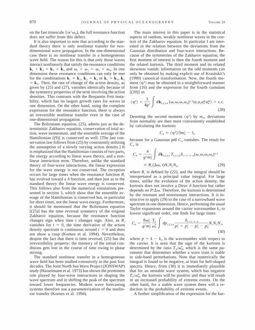
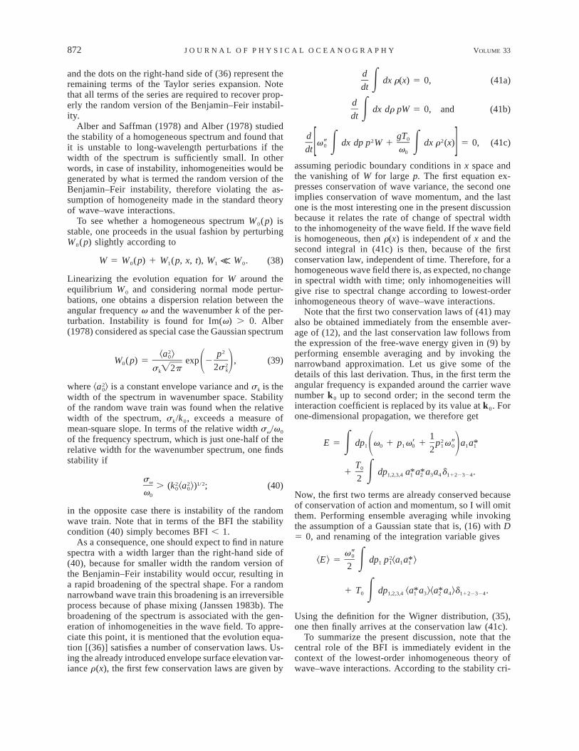
FIG. 3. Time evolution of spectral width for several values ofthe BFI. Corresponding results from homogeneous theory are alsoshown.

FIG. 4. Initial and final-time wavenumber spectrum according tothe Monte Carlo forecasting of waves (MCFW) using the nonlinearSchrodinger equation. Error bars give 95% confidence limits. Resultsfrom theory are also shown.

not evident that for the system under discussion theergodic hypothesis applies. This hypothesis implies re-placement of the ensemble average by a time average.However, if one happens to choose initial phases in away that is favorable for the generation of envelopesolitons, then there is a high probability that the solutionstays close to the envelope soliton branch and will hard-ly ever visit other parts of phase space. To guarantee arepresentative picture, we therefore decided to performNens runs, where for each run amplitude and phase aredrawn in an independent manner. In the remainder, onlyensemble-averaged results will be discussed. These arepresented graphically in the figures. To limit the numberof plots, each figure shows results from the numericalsimulations [usually denoted by Monte Carlo forecast-ing of waves (MCFW)], and corresponding results fromthe stochastic approach (labeled ‘‘theory’’). The theo-retical results are discussed in section 4.

In Fig. 3 I show the evolution of the spectral widthsk with dimensionless time t9 for several values of BFI.Here, sk is defined using integrals of the wave spectrumF over wavenumber p:

2dp p F(p)E2s 5 . (48)k

dp F(p)ENote that for simulations with the nonlinear Schrodingerequation this turned out to give a remarkably stableestimate of the width of the spectral peak, because thespectra vanish sufficiently rapidly for large p. Accordingto this simulation, there is a considerable broadening ofthe spectrum, which occurs on a fairly short timescaleof about 10 peak wave periods. In this case of one-dimensional propagation, the standard theory of non-

linear transfer would give no spectral change. Note thatsk shows in the early stages of time evolution an over-shoot followed by a rapid transition toward an equilib-rium value. The number of oscillations around this equi-librium value depends on the precise details of the dis-cretization scheme. In particular, more, larger-amplitudeoscillations are found for coarser spectral resolution.The overshoot is in agreement with results of Janssen(1983b), who studied the evolution of a single unstablemode in the context of inhomogeneous theory of wave–wave interactions. For sufficiently narrow spectra, over-shoot in the amplitude of the unstable mode was foundfollowed by a damped oscillation toward an equilibriumvalue. The damping timescale was found to depend onthe width of the spectrum, vanishing for small width.In physical terms, the damping is caused by phase mix-ing (or destructive interference), and its effect dependson wavenumber resolution. Note that other parameters,such as the kurtosis, show a similar time behavior.

As an example of spectral evolution, Fig. 4 showsfor BFI 5 1.40 the initial and final time–wavenumberspectrum. To give an idea about the representativenessof the results, 95% confidence limits, based on Nens 21 degrees of freedom, are shown as well. The broad-ening of the spectrum as caused by the nonlinear in-teractions is statistically significant. Although the spec-tral change should be symmetrical with respect to thecarrier wavenumber, that is, p 5 0, it is clear that thereare asymmetries present in the ensemble average of thenumerical results. However, these deviations are withinthe statistical uncertainty. To make sure of this, I redidthe case for BFI 5 1.40 but now with an ensemble sizeof 2000. As expected, statistical uncertainty was reducedby a factor of 2 while asymmetries were reduced aswell.

To examine whether the Monte Carlo results showevidence of a bifurcation at BFI 5 1, I plot in Fig. 5


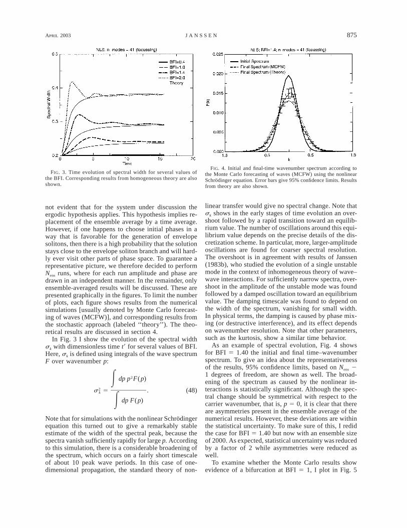
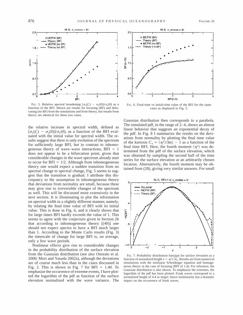
FIG. 5. Relative spectral broadening [sk( ) 2 sk(0)]/sk(0) as at9function of the BFI. Shown are results for focusing (BF) and defo-cusing (no BF) from the simulations and from theory, but results fromtheory are identical for these two cases.

FIG. 6. Final-time vs initial-time value of the BFI for the samecases as displayed in Fig. 5.

FIG. 7. Probability distribution function for surface elevation as afunction of normalized height x 5 h/ . Results are from numericalÏm0

simulations with the nonlinear Schrodinger equation and homoge-neous theory in the case of focusing (BFI of 1.4). For reference, theGaussian distribution is also shown. To emphasize the extremes, thelogarithm of the pdf has been plotted. Freak waves correspond to anormalized height of 4.4 or larger; hence nonlinearity has a dramaticimpact on the occurrence of freak waves.

the relative increase in spectral width, defined as[sk( ) 2 sk(0)]/sk(0), as a function of the BFI eval-t9uated with the initial value for spectral width. The re-sults suggest that there is only evolution of the spectrumfor sufficiently large BFI, but in contrast to inhomo-geneous theory of wave–wave interactions, BFI 5 1does not appear to be a bifurcation point, given thatconsiderable changes in the wave spectrum already startto occur for BFI 5 1/2. Although from inhomogeneoustheory one would expect a sudden transition from nospectral change to spectral change, Fig. 5 seems to sug-gest that the transition is gradual. I attribute this dis-crepancy to the assumption in inhomogeneous theorythat deviations from normality are small, because thesemay give rise to irreversible changes of the spectrumas well. This will be discussed more extensively in thenext section. It is illuminating to plot the informationon spectral width in a slightly different manner, namely,by relating the final time value of BFI with its initialvalue. This is done in Fig. 6, and it clearly shows thatfor large times BFI hardly exceeds the value of 1. Thisseems to agree with the conjecture given in Section 2bthat according to inhomogeneous theory [(40)] oneshould not expect spectra to have a BFI much largerthan 1. According to the Monte Carlo results (Fig. 3)the timescale of change for large BFI is, on average,only a few wave periods.

Nonlinear effects give rise to considerable changesin the probability distribution of the surface elevationfrom the Gaussian distribution (see also Onorato et al.2000; Mori and Yasuda 2002a), although the deviationsare of course much less than in the cases discussed inFig. 2. This is shown in Fig. 7 for BFI 5 1.40. Toemphasize the occurrence of extreme events, I have plot-ted the logarithm of the pdf as function of the surfaceelevation normalized with the wave variance. The

Gaussian distribution then corresponds to a parabola.The simulated pdf, in the range of 2–4, shows an almostlinear behavior that suggests an exponential decay ofthe pdf. In Fig. 8 I summarize the results on the devi-ations from normality by plotting the final time valueof the kurtosis C4 5 ^h4&/3 2 1 as a function of the2m0

final time BFI. Here, the fourth moment ^h4& was de-termined from the pdf of the surface elevation, whichwas obtained by sampling the second half of the timeseries for the surface elevation at an arbitrarily chosenlocation. Alternatively, the fourth moment may be ob-tained from (28), giving very similar answers. For small


FIG. 8. Normalized kurtosis as function of the final-time BFI. Thetheoretical result for defocusing can be obtained from the results offocusing by a reflection with respect to the x axis.

FIG. 9. Probability distribution function for surface elevation as afunction of normalized height x 5 h/ . Results are from numericalÏm0

simulations with the nonlinear Schrodinger equation and homoge-neous theory in the case of defocusing (BFI of 1.4). For reference,the Gaussian distribution is also shown.

nonlinearity one would expect a vanishing kurtosis, butthe simulation still underestimates, as already men-tioned, the kurtosis by 2%. The kurtosis depends almostquadratically on the Benjamin–Feir index up to a valueclose to 1. This quadratic dependence will be explainedin the next section, when an interpretation of results isprovided. Near BFI 5 1, on the other hand, the kurtosisbehaves in a more singular fashion, because, in agree-ment with the discussion of Fig. 6, the Benjamin–Feirindex cannot pass the barrier near 1.

The nonlinear Schrodinger equation [(45)] for deep-water waves is an example in which nonlinearity leadsto focusing of wave energy and therefore counteractsthe dispersion by the linear term, which is proportionalto . The results from the numerical simulation dov00indeed suggest that, when nonlinearity is sufficientlystrong, focusing of energy occurs, giving considerableenhancements to the probability of extreme events, atleast when compared with the normal distribution. Inthe opposite case, when the nonlinear term has oppositesign, defocusing of wave energy occurs and one wouldexpect a reduction in the number of extreme events. Toshow this, I performed simulations with the nonlinearSchrodinger equation [(45)] but now with negative non-linear transfer coefficient (T0 5 2 ). Results of this3k0

case are shown in Figs. 5, 6, and 8; the logarithm ofthe pdf of the surface elevation is shown in Fig. 9. Theseplots show that in the case of defocusing the broadeningof the spectrum is less dramatic. Furthermore, the finaltime Benjamin–Feir index does not have a limiting valueof about 1. On the other hand, the kurtosis for this caseis negative, resulting, as can be seen from Fig. 9, in alarge reduction of the probability of extreme events. Thedependence of the kurtosis on BFI is different from thecase of focusing, because there are clear signs of sat-uration beyond BFI 5 1, whereas only in the range BFI

, 0.5 is there a quadratic dependence of kurtosis C4 onBFI.

b. Nonlinear transfer according to the Zakharovequation

The nonlinear Schrodinger equation gives the lowest-order effects of finite bandwidth on the evolution of aweakly nonlinear wave train. Dysthe (1979) investigatedthe consequences of next order in bandwidth and hefound a surprisingly large impact on the results for thegrowth rates of the modulational instability. Similarly,Crawford et al. (1981) studied the stability of a uniformwave train using the complete Zakharov equation, whichretains all of the high-order dispersion effects. In gen-eral, growth rates are reduced when compared with re-sults from the nonlinear Schrodinger equation; there-fore, according to the Zakharov and Dysthe equations,a uniform wave train is less unstable. In fact, growthrates and thresholds for instability were in better agree-ment with experimental results of Benjamin and Feir(1967) and Lake et al. (1977) (see also Janssen 1983a).The Zakharov and Dysthe equations have, in addition,the interesting property that the nonlinear transfer co-efficient and the angular frequencies are not symmetricalwith respect to the carrier wavenumber. It will be seenthat this has important consequences for the spectralshape.

The Dysthe equation follows from the Zakharovequation by expanding angular frequency to third orderin the modulation wave number p while the interactioncoefficient T is expanded up to first order in p. Fornarrowband wave trains it gives an accurate descriptionof the sea state. However, wave spectra may become sobroad that the narrowband approximation becomes in-


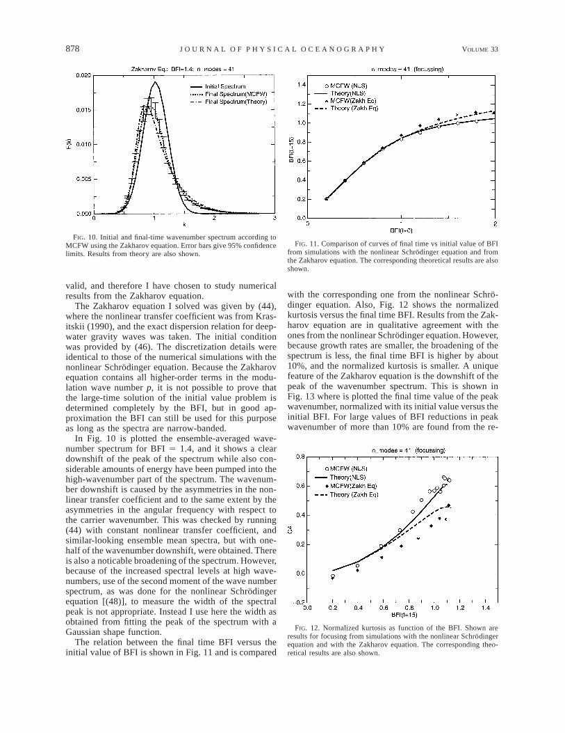
FIG. 10. Initial and final-time wavenumber spectrum according toMCFW using the Zakharov equation. Error bars give 95% confidencelimits. Results from theory are also shown.

FIG. 11. Comparison of curves of final time vs initial value of BFIfrom simulations with the nonlinear Schrodinger equation and fromthe Zakharov equation. The corresponding theoretical results are alsoshown.

FIG. 12. Normalized kurtosis as function of the BFI. Shown areresults for focusing from simulations with the nonlinear Schrodingerequation and with the Zakharov equation. The corresponding theo-retical results are also shown.

valid, and therefore I have chosen to study numericalresults from the Zakharov equation.

The Zakharov equation I solved was given by (44),where the nonlinear transfer coefficient was from Kras-itskii (1990), and the exact dispersion relation for deep-water gravity waves was taken. The initial conditionwas provided by (46). The discretization details wereidentical to those of the numerical simulations with thenonlinear Schrodinger equation. Because the Zakharovequation contains all higher-order terms in the modu-lation wave number p, it is not possible to prove thatthe large-time solution of the initial value problem isdetermined completely by the BFI, but in good ap-proximation the BFI can still be used for this purposeas long as the spectra are narrow-banded.

In Fig. 10 is plotted the ensemble-averaged wave-number spectrum for BFI 5 1.4, and it shows a cleardownshift of the peak of the spectrum while also con-siderable amounts of energy have been pumped into thehigh-wavenumber part of the spectrum. The wavenum-ber downshift is caused by the asymmetries in the non-linear transfer coefficient and to the same extent by theasymmetries in the angular frequency with respect tothe carrier wavenumber. This was checked by running(44) with constant nonlinear transfer coefficient, andsimilar-looking ensemble mean spectra, but with one-half of the wavenumber downshift, were obtained. Thereis also a noticable broadening of the spectrum. However,because of the increased spectral levels at high wave-numbers, use of the second moment of the wave numberspectrum, as was done for the nonlinear Schrodingerequation [(48)], to measure the width of the spectralpeak is not appropriate. Instead I use here the width asobtained from fitting the peak of the spectrum with aGaussian shape function.

The relation between the final time BFI versus theinitial value of BFI is shown in Fig. 11 and is compared

with the corresponding one from the nonlinear Schro-dinger equation. Also, Fig. 12 shows the normalizedkurtosis versus the final time BFI. Results from the Zak-harov equation are in qualitative agreement with theones from the nonlinear Schrodinger equation. However,because growth rates are smaller, the broadening of thespectrum is less, the final time BFI is higher by about10%, and the normalized kurtosis is smaller. A uniquefeature of the Zakharov equation is the downshift of thepeak of the wavenumber spectrum. This is shown inFig. 13 where is plotted the final time value of the peakwavenumber, normalized with its initial value versus theinitial BFI. For large values of BFI reductions in peakwavenumber of more than 10% are found from the re-


FIG. 13. Final-time peak wavenumber downshift vs BFI. Shown isa comparison between numerical simulation results from the Zak-harov equation and theory.

sults of the numerical simulations, but the dependenceof the downshift in peak wavenumber on BFI is notsmooth. This is caused by the fact that the ensemble-averaged spectra do not always have a well-definedspectral peak.

4. Interpretation of numerical results

In the previous section I have discussed results fromthe Monte Carlo simulation of the nonlinear Schrodingerequation and the Zakharov equation. These results showthat on average there is a rapid broadening of the wavespectrum while nonlinearity gives rise to considerabledeviations from Gaussian statistics. The question nowis whether the average of the Monte Carlo results maybe obtained in the framework of a simple theoreticaldescription. In section 2 I discussed two attempts toachieve this. The first one is the standard theory ofwave–wave interactions, extended with the effects ofnonresonant four-wave interactions. This approach as-sumes a homogeneous wave field but allows for devi-ations from the Gaussian sea state. The second theoryis the inhomogeneous theory of wave–wave interac-tions, which assumes that effects of inhomogeneity inthe wave field are dominant while deviations from nor-mality only play a minor role. This approach seems tobe an ideal starting point for treating inhomogeneousand nonstationary phenomena such as freak waves be-cause it describes the random version of the Benjamin–Feir instability. Let us therefore first discuss the validityof inhomogeneous theory using results from the MonteCarlo forecasting of ocean waves obtained from the non-linear Schrodinger equation.

According to inhomogeneous theory the broadeningof the wave spectrum is caused by the inhomogeneityof the wave field. This is clearly expressed by the con-servation law [(41c)] and is explained in the discussion

that follows. From this conservation law, one may there-fore obtain a measure of inhomogeneity of the wavefield, namely,

2I 5 I /I ,2 1 (49)

where

I 5 dx r(x) and (50)1 E2I 5 dx r (x). (51)2 E

Here, the integrals over space are weighted by thesize of the domain, and using the definitions for r [(37)]and the Wigner distribution [(35)] one may express theinhomogeneity measure I in terms of the correlationfunction B(n, m, t) as

2v0I 5 B(p, 0), and (52)O1 g p

22v0I 5 B(p, m)B*(p9, m). (53)O2 1 2g p,p9,m

The correlation functions B(p, m) may be readily ob-tained from the numerical results for the complex am-plitude a(k, t) after ensemble averaging. For a homo-geneous wave field B(p, m) 5 N(p)d(m); hence I2 5

, or I 5 1.2I1

The initial conditions used in the numerical simula-tion of waves have been chosen in such a way that thesea state corresponds to a Gaussian one. As a conse-quence, because the complex amplitudes a(k, t) are notcorrelated, this implies that initially the sea state is ho-mogeneous as well (Komen et al. 1994). However, thewave ensemble consists of a finite number of members,and this means that the initial probability distributionis not a perfect Gaussian (e.g., the kurtosis is slightlyunderestimated) but it also means that the initial con-ditions are slightly inhomogeneous. According to theinhomogeneous theory, the perturbations should growexponentially in time, resulting in, for example, a broad-ening of the wave spectrum.

For BFI 5 1.4, the evolution in time of the inho-mogeneity I is shown in Fig. 14. Initially, inhomoge-neity is small but grows rapidly in the course of time,which is then followed by an oscillation around the level1.004. This level of inhomogeneity and the variationwith time is, however, extremely small (note that forthe case of Fig. 1a, I is on the order of 3), and it cannotexplain the large changes in the wavenumber spectrumseen in the numerical simulations.

In addition, according to the inhomogeneous theory,the conservation law of (41c) should be satisfied. Insection 3b it was explained that this conservation lawfollows from the conservation of Hamiltonian, assumingthat deviations from normality may be ignored. It is ofinterest, of course, to test whether it is justified to ignore


FIG. 14. Time evolution of a measure for inhomogeneity, I, for twodifferent ensemble sizes, according to the nonlinear Schrodingerequation.

FIG. 15. Time evolution of Hamiltonian E of the nonlinear Schro-dinger equation. Also shown are time evolution of E according tolowest-order inhomogeneous theory (Eapprox) and according to ho-mogeneous theory that includes the fourth cumulant. Also shown arethe nonlinear contributions to E for a strictly Gaussian state [NL (C4

5 0)] and including all higher-order cumulants (NL 1 C4).effects of the fourth cumulant. To that end, Fig. 15 com-pares the evolution in time of the Hamiltonian as ob-tained from the numerical simulation (this will be calledthe ‘‘exact’’ Hamiltonian from now on) with the Ham-iltonian according to inhomogeneous theory. Althoughthe exact Hamiltonian is a constant (at least up to fivesignificant digits), it is clear that the approximate Ham-iltonian is not conserved when evaluated using the nu-merical results. In fact, there are large deviations as theapproximate Hamiltonian becomes negative, whereasthe exact Hamiltonian is positive definite. The disagree-ment between the approximate and the exact Hamilto-nian is caused by the neglect of the higher-order cu-mulants. This is immediately clear from Fig. 15 in whichthe nonlinear contribution to the Hamiltonian accordingto lowest-order inhomogeneous theory [called approx-imate; NL (c4 5 0)] is compared with the correspondingnonlinear contribution that includes higher-order cu-mulants (called exact; NL 1 c4). The approximate non-linear contribution hardly varies with time, which is inagreement with the results from Fig. 14 that effects ofinhomogeneity are small. The exact nonlinear contri-bution shows a significant variation with time. The dif-ferences between exact and approximate are consider-able, and therefore it is not justified to ignore effects ofdeviations from normality in a simple theoretical de-scription of the evolution of the sea state. As a matterof fact, the deviations from normality are the main rea-son for the spectral broadening as the time-varying non-linear contribution to the Hamiltonian, including effectsof the fourth-order cumulant, just compensates for thechanges with time of the linear part of the wave energy.Clearly, according to the Monte Carlo simulations thelinear wave energy is not conserved.

The previous discussion therefore suggests that ef-fects of the deviations from normality are important,which may explain why there is no bifurcation at BFI

5 1 as is suggested by inhomogeneous theory (Fig. 5).Alternatively, there could be another possible reason forthe discrepancy between the inhomogeneous theory andthe numerical results. The evidence for a bifurcation atBFI 5 1 follows from a linear stability analysis; there-fore the perturbation of the homogeneous spectrum isassumed to be small. In the numerical simulations theperturbation is not prescribed a priori and its amplitudeis determined by the full nonlinear evolution equation.The initial size of the perturbation is, however, deter-mined in an indirect way by the ensemble size, becausethe larger the ensemble is, the closer one approaches toconditions for a homogeneous sea state. This is evidentin Fig. 14 in which the inhomogeneity I is smaller forlarger ensemble size. I therefore performed Monte Carlosimulations with different ensemble size, namely, forNens 5 50 and Nens 5 2000, but almost identical resultsfor, for example, the relative increase in spectral widthas a function of BFI were found. Although this doesnot present conclusive evidence, it does suggest that theinitial size of the perturbations is small enough and thatthe main reason for the absence of a bifurcation at BFI5 1 is the neglect of deviations from normality.

In summary, it has been shown that, in the inho-mogeneous theory of four-wave interactions, effects ofthe generation of the fourth cumulant cannot be ignored.At the same time it has been shown that the numericalensemble of ocean waves may be regarded to good ap-proximation as a homogeneous ensemble. Hence, thestandard theory of four-wave interactions (extended byincluding nonresonant interactions), which assumes ahomogeneous wave field, may be a good candidate toexplain the results of the numerical simulations in sec-tion 3.

Therefore, the Boltzmann equation [(25)] was used


to evolve the action density N(k) for the same cases aspresented in section 3. The differential equation wassolved with a Runge–Kutta method with variable timestep, and the continuous problem was discretized in thesame way as was done in the case of the solution of theZakharov equation. Run times using the homogeneoustheory are typically two orders of magnitudes faster thanwhen following the ensemble approach.

In contrast to inhomogeneous theory, the standardtheory gives a much better approximation to the exactHamiltonian as shown in Fig. 15. There are, as shouldbe, small differences because the standard theory is anapproximation as well, given that both effects of in-homogeneity and the sixth cumulant have been neglect-ed. Further results from the discretized version of thehomogeneous theory are compared with the ones fromthe simulations with the nonlinear Schrodinger equationin Figs. 3–8.

From Fig. 3, which shows the evolution in time ofthe spectral width for several values of the BFI, it isseen that for large times there is good agreement be-tween homogeneous theory and the ensemble-averagedresults from the Monte Carlo simulations. For shorttimes it is, however, evident that (25) does not showthe overshoot found in the numerical simulations. Alikely reason for the absence of overshoot found in thetheoretical calculations is the assumption that the actiondensity varies slowly as compared with the timescaleimplied by the resonance function Ri(Dv, t). Both thenumerical simulations and homogeneous theory showfor short times a rapid broadening of the wave spectrum,which for large times is followed by a transition towardsa steady state. The evolution toward a steady state canbe understood as follows: First, it should be noted that,according to section 2c, for one-dimensional propaga-tion there is no nonlinear transfer because of resonantnonlinear interactions. Now, initially the resonancefunction Ri(Dv, t) will be wide so that nonresonantwave–wave interactions are allowed to modify the ac-tion density spectrum. After about 5–10 wave periods,however, the resonance function becomes progressivelynarrower until it becomes approximately a d function;hence only resonant waves are selected. In that eventthere is no change of the action density spectrum pos-sible anymore so that for large times a steady state isachieved.

An example of the comparison between theoreticaland simulated spectra is given in Fig. 4. There is a fairagreement between the two. However, it should be men-tioned that typically the simulated spectrum is slightlymore peaked than the theoretical one despite the factthat there is a close agreement in spectral width. Thisagreement in spectral width between theory and simu-lation is also very much evident in the Figs. 5 and 6over the full range of the initial value of BFI. In par-ticular, note that there is close agreement between theupper limit of the final time BFI from theory and thesimulation. Hence, homogeneous theory also provides

an explanation of why there is a lower bound to spectralwidth.

We therefore have the curious situation in which bothhomogeneous and inhomogeneous theory explain whythere is a lower bound to spectral width as found in thenumerical simulations. However, because it has beenshown that inhomogeneities only play a minor role inthe numerical simulations it follows that only homo-geneous theory provides a proper explanation. In situobservations from the North Sea seem to indicate thepresence of a lower bound to spectral width as well (see,e.g., Janssen 1991). Although it is impossible to proveat present that at sea inhomogeneities do not play a role,homogeneous theory even seems to give a plausibleexplanation of the lower bound found at sea.

As discussed in section 2c, nonlinearity gives rise todeviations from the normal distribution. I determinedthe normalized kurtosis using (29), which is obtainedfrom the fourth cumulant D. Introducing the normalizedheight x 5 h/ , the pdf of the normalized surfaceÏm0

elevation x is then given by (see also Mori and Yasuda2002b)

41 dp(x) 5 1 1 C f , (54)4 041 28 dx

where f 0 is given by the normal distribution

21 xf (x) 5 exp 2 . (55)0 1 22Ï2p

Equation (54) follows from an expansion of the pdf pin terms of orthogonal functions (d/dx)nf 0. Here, n iseven because of the symmetry of the Zakharov equation.The expansion coefficients are then obtained by deter-mining the first, second, and fourth moments. For therange of BFI studied in this paper, it was verified thathigher moments only gave a small contribution to theshape of the pdf p(x). The pdf according to theory iscompared in Fig. 7 with the simulated one, and a goodagreement is obtained, even for extreme sea state con-ditions. Clearly, in the case of nonlinear focusing, theprobability of extreme states is, as expected, larger whencompared with the normal distribution. In Fig. 8, the-oretical and simulated final-time kurtosis is plotted asfunction of the final-time BFI. A good agreement be-tween the two results is obtained, even close to thelimiting value of the final-time BFI. For BFI , 1, bothsimulated and theoretical kurtosis depend in an almostquadratic fashion on BFI, in agreement with the simpleestimates of C4 given in section 2c [(31)].

In the case of nonlinear focusing, a good agreementbetween the numerical simulations and the homoge-neous theory has been obtained, even for extreme valuesof the Benjamin–Feir index. Here, it should be empha-sized that at sea BFI has typical values of 0.5 or less,and only occasionally are values on the order of 1reached. We have performed simulations to values ofBFI of up to 3 and, even for these extreme conditions


(having large values of kurtosis, for example), a rea-sonable agreement is obtained. This is surprising be-cause the homogeneous theory was derived under theassumption of small deviations from normality.

In the case of nonlinear defocusing, the range of va-lidity of homogeneous theory is much more restricted.This is made plainly clear in Figs. 5, 6, 8, and 9, whereresults from the simulations and homogeneous theoryare compared for the case of nonlinear defocusing. Tobe able to interpret this comparison, note that homo-geneous theory does not distinguish between focusingand defocusing, because the nonlinear transfer is in-dependent of the sign of the interaction coefficient T.Only the kurtosis depends on the sign of T. Judgingfrom Figs. 5, 6, and 8, the range of validity of homo-geneous theory is restricted to BFI , 0.6. In particular,for large BFI there are large qualitative deviations inthe kurtosis of the pdf: from the numerical simulationsthere are clear signs of saturation in kurtosis, but thereis no indication of saturation in the results from ho-mogeneous theory. In addition, in the case of nonlineardefocusing the kurtosis is negative so that for large nor-malized elevation x the pdf given in (54) may becomenegative. This is clearly unrealistic, and to correct thisundesirable property of homogeneous theory one needs,for large BFI, to take into account the effects of higher-than-fourth-order cumulants as well. It is believed thisis the main reason why homogeneous theory has sucha restricted validity in this case. In the opposite case ofnonlinear focusing, the kurtosis is positive, giving forlarge x a positive correction to the normal distribution.The pdf of the surface elevation is therefore positive,at least for the cases that have been studied here, andas a consequence homogeneous theory has a much larg-er range of validity.

Last, I applied homogeneous theory to the Zakharovequation. Results are compared with the numerical sim-ulations in Figs. 10, 11, 12, and 13. There is a fairagreement between simulated and theoretical spectrum(Fig. 10), between simulated and theoretical final-timeBFI index (Fig. 11), and in normalized kurtosis (Fig.12). Less favorable is the agreement between simulatedand theoretical peak wavenumber, as shown in Fig. 13.The theoretical results show a smooth dependence ofwavenumber downshift on BFI, giving shifts of 20% ormore for large values of BFI. However, the simulationshows more scatter while the downshift is at most 15%.The reason for the scatter in the simulated results isprobably that the peak of the wavenumber spectrum isnot always well defined. In contrast, homogeneous the-ory gives a smoother spectrum and a well-defined peakof the spectrum.

5. Conclusions

Present-day wave forecasting systems are based on adescription of the ensemble-averaged sea state. In thisapproach, the wavenumber spectrum plays a central role

and its evolution follows from the energy balance equa-tion. The question discussed here is whether it is pos-sible to make statements, necessarily of a statistical na-ture, on the occurrence of extreme events such as freakwaves.

To show that this is possible, the following approachhas been adopted. The starting point is a deterministicset of equations, namely, the Zakharov equation or itsnarrowband limit, the nonlinear Schrodinger equation.There is ample evidence that these equations admit freakwave–type solutions. These freak waves occur when thewaves are sufficiently steep, because nonlinear focusingmay then overcome the spreading of energy by lineardispersion. For the same reason, the Benjamin–Feir in-stability occurs. As shown in Fig. 1, the occurrence offreak waves depends in a sensitive manner on the choiceof the initial phase of the waves. In addition, on theopen ocean, waves propagate from different locationstoward a certain point of interest and may therefore beregarded as independent. Hence, for open-ocean appli-cations, the random-phase approximation seems to beappropriate. I therefore simulated the evolution of anensemble of ocean waves by running a deterministicmodel with random initial phase. These Monte Carlosimulations are expensive (typically, the size of the en-semble is 500) so that the study is restricted to the caseof one-dimensional propagation only.

The ensemble average of the results from the MonteCarlo simulations shows that when the Benjamin–Feirindex is sufficiently large (as occurs for the combinationof narrow spectra and steep waves) the wave spectrumbroadens while at the same time considerable deviationsfrom the Gaussian pdf are found. In the case of theZakharov equation, the spectral change is even asym-metrical with respect to the peak of a symmetrical spec-trum, giving a downshift of the peak wavenumber whileas a consequence of the conservation of wave actionand wave energy considerable amounts of energy arebeing pumped into the high-wavenumber part of thespectrum. These spectral changes occur on a short time-scale, typically on the order of 10 wave periods. Thistimescale is comparable to the Benjamin–Feir timescale.

The standard homogeneous theory of resonant non-linear transfer does not give spectral change in the caseof one-dimensional propagation. This theory was there-fore extended to allow for nonresonant interactions aswell, because the nonlinear focusing related to the Ben-jamin-Feir instability is an example of a nonresonantfour-wave interaction. This nonlinear four-wave transferis associated with the generation of higher-order cu-mulants such as the kurtosis. Deviations of the surfaceelevation pdf from the normal distribution can thereforebe expressed in terms of a six-dimensional integral in-volving the cube of the action spectrum [(29)]. In thecase of nonlinear focusing, there is, for a large rangeof values of the BFI, a good agreement between theensemble-averaged results from the numerical simula-tions and homogeneous theory. This is in particular true


for the broadening of the spectrum, the spectral shape,and the estimation of the kurtosis. In comparison withthe simulations, theory overestimates, however, the peakwavenumber downshift.

Homogeneous theory also explains why for one-di-mensional propagation the wave spectrum evolves to-ward a steady state. The resonance function evolvesrapidly toward a d function; hence for large times onlyresonant wave–wave interactions are selected that in onedimension do not give rise to spectral change. This isin sharp contrast with the case of two-dimensional prop-agation. No trend toward a steady state is expected inthat case because resonant four-wave interactions docontribute to a change in the spectrum.

The extended version of the homogeneous four-wavetheory has two timescales, a fast one on which the non-resonant interactions take place and a long timescale onwhich the resonant interactions occur. The nonresonantinteractions play a role similar to that of transients inthe solution of an initial-value problem. They are simplygenerated because initially there is a mismatch betweenthe choice of the probability distribution of the waves,a Gaussian, and between the initial choice of the wavespectrum, representing a sea state with narrowband,steep nonlinear waves. For example, if one could choosea probability distribution function which is in equilib-rium with the nonlinear sea state (theoretically one can,by the way), then nonresonant interactions would notcontribute. Only resonant wave–wave interactions willthen give rise to nonlinear transfer. In the general casefor which there is a finite mismatch between pdf andwave spectrum, the nonresonant contribution will dieout very quickly owing to phase mixing but will, nev-ertheless, as we have seen, result in considerable chang-es in the wave spectrum. The question therefore iswhether there is a need to include effects of nonresonantinteractions. This depends on the application. In wave-tank experiments, where one can program a wave makerto produce the initial conditions used in this paper, itseems that effects of nonresonant transfer need to betaken account for. For the open-ocean case this is notclear. The point is that in nature the combination of steepwaves and a strictly Gaussian distribution most likelydoes not occur. Changes in nature are expected to bemore gradual so that the mismatch between pdf andwave spectrum is small. Only when a wind starts blow-ing suddenly, hence for short fetches and duration, areeffects of nonresonant interactions expected to be rel-evant. More research in this direction is, however, re-quired.

The results from Monte Carlo simulations do not pro-vide evidence that there are significant deviations fromhomogeneity of the ensemble of waves. Deviations fromnormality are found to be much more important. Nev-ertheless, it cannot be concluded from the present studythat the inhomogeneous approach of Alber and Saffman(1978) is not relevant for real ocean waves. For example,effects of inhomogeneity might be relevant in fetch-

limited, rapidly varying circumstances. However, its ef-fects are expected to be small, and therefore only thelowest-order approximation, as given explicitly in (36),needs to be retained.

For real ocean waves, not only four-wave interactionsdetermine the evolution of the wave spectrum. Windinput and dissipation due to white-capping are relevant,and these processes may affect the kurtosis of the seasurface as well. However, it has been shown in this paperthat in particular the nonresonant nonlinear transfer actson a short timescale that is much shorter then the time-scales associated with wind input and dissipation sourcefunctions used in wave forecasting (Komen et al. 1994).Hence, one would expect that the expression for kurtosisfound in this paper [(29)] should be relevant in nature.Nevertheless, nonlinear focusing may result in steepwaves. If their steepness exceeds a certain threshold,one would expect a significant amount of wave break-ing, thus limiting the height of these waves, and af-fecting the extreme statistics. A realistic, deterministicmodel of wave breaking is needed to assess the impor-tance of wave breaking in these circumstances. It maybe more effective, however, to try to compare resultsfrom the present approach directly with observations ofextremes collected over a long period.

Acknowledgments. The author acknowledges usefuland stimulating discussions with Miguel Onorato. Hispresentation during the 2001 Wise meeting in Canadagave stimulus to have a fresh look at wave–wave in-teractions and freak waves. Furthermore, the authorthanks Theo van Steyn for providing the Runge–Kuttasoftware for accurate integration of a set of ordinarydifferential equations. Last, the author thanks AnthonyHollingsworth and Martin Miller for critically readingthe manuscript.

REFERENCES

Alber, I. E., 1978: The effects of randomness on the stability of two-dimensional surface wave trains. Proc. Roy. Soc. London, A363,525–546.

——, and P. G. Saffman, 1978: Stability of random nonlinear deep-water waves with finite bandwidth spectra. TRW Defense andSpace System Group Rep. 31326-6035-RU-00, 89 pp.

Benjamin, T. B., and J. E. Feir, 1967: The disintegration of wavetrainson deep water. Part 1: Theory. J. Fluid Mech., 27, 417–430.

Benney, D., and A. C. Newell, 1967: The propagation of nonlinearwave envelopes. J. Math. Phys., 46, 133–139.

Caponi, E. A., P. G. Saffman, and H. C. Yuen, 1982: Instability andconfined chaos in a nonlinear dispersive wave system. Phys.Fluids, 25, 2159–2166.

Cohen, B. I., K. M. Watson, and B. J. West, 1976: Some propertiesof deep water solitons. Phys. Fluids, 19, 345–350.

Crawford, D. R., P. G. Saffman, and H. C. Yuen, 1980: Evolution ofa random inhomogeneous field of nonlinear-deep-water gravitywaves. Wave Motion, 2, 1–16.

——, B. M. Lake, P. G. Saffman, and H. C. Yuen, 1981: Stability ofweakly nonlinear deep-water waves in two and three dimensions.J. Fluid Mech., 105, 177–191.

Davey, A., 1972: The propagation of a weak nonlinear wave. J. FluidMech., 53, 769–781.


Davidson, R. C., 1972: Methods in Nonlinear Plasma Theory. Ac-ademic Press, 356 pp.

Dean, R. G., 1990: Freak waves: A possible explanation. Water WaveKinematics, A. Torum and O. T. Gudmestad, Eds., Kluwer, 609–612.

Draper, L., 1965: ‘‘Freak’’ ocean waves. Mar. Obs., 35, 193–195.Dysthe, K. B., 1979: Note on a modification to the nonlinear Schro-

dinger equation for application to deep water waves. Proc. Roy.Soc. London, A369, 105–114.

Hasimoto, H., and H. Ono, 1972: Nonlinear modulation of gravitywaves. J. Phys. Soc. Japan, 33, 805–811.

Hasselmann, K., 1962: On the non-linear energy transfer in a gravity-wave spectrum. Part 1: General theory. J. Fluid Mech., 12, 481.

——, and Coauthors, 1973: Measurements of wind-wave growth andswell decay during the Joint North Sea Wave Project (JON-SWAP). Dtsch. Hydrogr. Z. Suppl., 8A (12), 95 pp.

Janssen, P. A. E. M., 1983a: On a fourth-order envelope equation fordeep-water waves. J. Fluid Mech., 126, 1–11.

——, 1983b: Long-time behaviour of a random inhomogeneous fieldof weakly nonlinear surface gravity waves. J. Fluid Mech., 133,113–132.

——, 1991: On nonlinear wave groups and consequences for spectralevolution. Directional Ocean Wave Spectra, R. C. Beal, Ed.,The Johns Hopkins University Press, 46–52.

——, and G. J. Komen, 1982: Modification of the surface elevationprobability distribution in ocean swell by nonlinear spectralbroadening. J. Geophys. Res., 87, 4155–4162.

Komen, G. J., L. Cavaleri, M. Donelan, K. Hasselmann, S. Hassel-mann, and P. A. E. M. Janssen, 1994: Dynamics and Modellingof Ocean Waves. Cambridge University Press, 554 pp.

Krasitskii, V. P., 1990: Canonical transformation in a theory of weaklynon-linear waves with a nondecay dispersion law. Sov. Phys.JETP, 71, 921–927.

——, and V. A. Kalmykov, 1993: Four-wave reduced equations forsurface gravity waves. Izv. Atmos. Phys., 29, 222–228.

Lake, B. M., H. C. Yuen, H. Rungaldier, and W. E. Ferguson, 1977:Nonlinear deep-water waves: Theory and experiment. Part 2:Evolution of a continuous wave train. J. Fluid Mech., 83, 49–74.

Lavrenov, I., 1998: The wave energy concentration at the AgulhasCurrent of South Africa. Nat. Haz., 17, 117.

Longuet-Higgins, M. S., 1978: The instabilities of gravity waves offinite amplitude in deep-water. II. Subharmonics. Proc. Roy. Soc.London, A360, 489–505.

Martin, D. U., and H. C. Yuen, 1980: Quasi-recurring energy leakagein the two-space-dimensional nonlinear Schrodinger equation.Phys. Fluids, 23, 881–883.

Mori, N., and T. Yasuda, 2002a: Effects of high-order nonlinear in-

teractions on unidirectional wave trains. Ocean Eng., 29, 1233–1245.

——, and ——, 2002b: A weakly non-gaussian model of wave dis-tribution for random wave train. Ocean Eng., 29, 1219–1231.

Onorato, M., A. R. Osborne, M. Serio, and T. Damiani, 2000: Oc-currence of freak waves from envelope equations in randomocean wave simulations. Rogue Waves 2000, M. Olagnon andG. A. Athanassoulis, Eds., Springer-Verlag, 181–191.

——, ——, ——, and S. Bertone, 2001: Freak waves in randomoceanic sea states. Phys. Rev. Lett., 86, 5831–5834.

Osborne, A. R., M. Onorato, and M. Serio, 2000: The nonlineardynamics of rogue waves and holes in deep water gravity wavetrains. Phys. Lett., 275A, 386–393.

Ostrowskii, L. A., 1967: Propagation of wave packets and space-timeself-focussing in a nonlinear medium. Sov. Phys. JETP, 24, 797–800.

Stokes, G. G., 1847: On the theory of oscillatory waves. Math. Phys.Pap., 1, 197–229.

Tanaka, M., 1992: The role of modulational instability in the for-mation of wave groups. Breaking Waves, M. L. Banner and R.H. J. Grimshaw, Eds., Springer Verlag, 237–242.

Trulsen, K., and K. Dysthe, 1997: Freak waves—a three-dimensionalwave simulation. Proceedings of the 21st Symposium on NavalHydrodynamics, E. P. Rood, Ed., National Academy Press, 550–558.

Tucker, M. J., P. G. Challenor, and D. J. T. Carter, 1984: Numericalsimulation of a random sea: A common error and its effect uponwave group statistics. Appl. Ocean Res., 6, 118–122.

Wigner, E., 1932: On the quantum correction for thermodynamicequilibrium. Phys. Rev., 40, 749–759.

Wolfram, J., B. Linfoot, and P. Stansell, 2000: Long- and short-termextreme wave statistics in the North Sea: 1994–1998. RogueWaves 2000, M. Olagnon and G. A. Anthanassoulis, Eds.,Springer-Verlag, 341–347.

Yuen, H. C., and W. E. Ferguson, 1978: Relationship between Ben-jamin–Feir instability and recurrence in the nonlinear Schro-dinger equation. Phys. Fluids, 21, 1275–1278.

——, and B. M. Lake, 1982: Nonlinear dynamics of deep watergravity waves. Adv. Appl. Mech., 22, 67–229.

Zakharov, V. E., 1968: Stability of periodic waves of finite amplitudeon the surface of a deep fluid. J. Appl. Mech. Tech. Phys., 9,190–194.

——, and N. N. Filonenko, 1968: The energy spectrum for randomsurface waves. Dokl. Acad. Sci. USSR, 170, 1291–1295.

——, and A. B. Shabat, 1972: Exact theory of two-dimensional self-focussing and one-dimensional self-modulating waves in non-linear media (English translation). Sov. Phys. JETP, 34, 62.

——, and A. M. Rubenchik, 1974: Instability of waveguides andsolitons in nonlinear media (English translation). Sov. Phys.JETP, 38, 494.

jpo_2003_4

Documents

wave energy

linear wave theory

abstractfourwave interactions

extreme wave events

varying wave train

suchextreme wave phenomena

freak wave phenomena

occurrence of freak