journée restitution des travaux de thèses du programme ... · une pathologie (cancers, maladies...

Journée restitution des travaux de

thèses du programme

FUTUR & RUPTURES

15 février 2018

Posters

Journée Futur & Ruptures Jeudi 15 février 2018

Posters

Ecole Titre de la thèse Encadrant Thésard

1 Eurecom Soft Cache Hits: Alternative Content

Recommendations

Thrasyvoulos

Spyropoulos

Theodore

Giannakas

2 IMT Atlantique Incremental learning of affordances using interactive

and strategical algorithms Maï Nguyen

Alexandre

Manoury

3 IMT Atlantique

Conception d’un nez électronique

pour la détection de pathologies

Application à la détection d’insuffisance rénale

Cyril Lahuec

Laurent Dupont Paul Le Maout

4 IMT Atlantique Emergence of Long Term Associative Memories in

Recurrent Hebbian Networks Under Noise

Charlotte

Langlais Eliott Coyac

5 IMT Lille Douai

Understanding the affective and stylistic human

motion

From the definition of style to its recognition Stakeholders

Hazem

Wannous -

Jean-Philippe

Vandeborre

Sarah Ribet

6 Télécom

PariTech

Système de Localisation 3D Indoor par Radar

Multistatique UWB

Jean-

Christophe

Cousin - Nel

Samama

Nour Awarkeh

7 Télécom

ParisTech

Cooperative Communications in very large cellular

Networks.

Nearest Neighbour Cooperation

Giovanidis

Anastasios

Luis David

Álvarez

Corrales

8 Télécom

ParisTech

Gestion de ressources photoniques pour l’application

aux réseaux de communications quantique

Isabelle

Zaquine

Julien

Trapateau

9 Télécom

ParisTech Trust based secure routing for the Internet of Things Anis Laouiti Asma Lahbib

10 Télécom

SudParis

Towards Testing and Verification in Software Defined

Networks

Djamal

Zeghlache -

Natalia Kushik

Asma Beriri

11 Télécom Ecole

de Management

Personal data and regulation

Empirical and experimental approach Grazia Cecere Vincent Lefrère

Thesis context

We aim for a robot capable of planning and performing tasks in a real life environment with a

limited prior knowledge, by discovering and learning affordances.

► Problems:

► Approach: active exploration and long life learning, in order to learn how to

recognize affordances from low level visual features

Incremental learning of

affordances using interactive

and strategical algorithms

Actors

Authors

Contact : [email protected]

15

Fé

vri

er

20

18

Jo

urn

ée

Fu

tur

& R

up

ture

s

P

ari

s

Alexandre Manoury

Thesis supervisor:

Mai Nguyen

Thesis director:

Cédric Buche

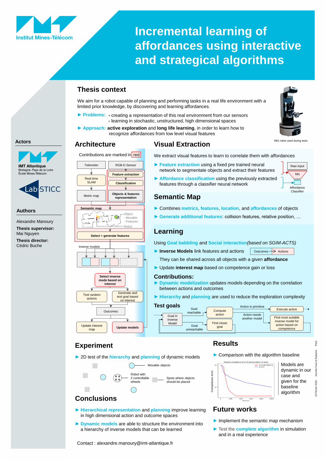
Architecture

RGB-D Sensor

Feature extraction

Real time

SLAM

Visual Extraction

We extract visual features to learn to correlate them with affordances

Metric map Objects & features

representation

Telemeter

Outcomes

Semantic Map

► Combines metrics, features, location, and affordances of objects

► Generate additional features: collision features, relative position, …

Results

► Comparison with the algorithm baseline

Conclusions

► Hierarchical representation and planning improve learning

in high dimensional action and outcome spaces

► Dynamic models are able to structure the environment into

a hierarchy of inverse models that can be learned

Classification

Semantic map

Inverse models

Test random

actions

Generate and

test goal based

on interest

Select inverse

mode based on

interest

Update interest

map Update models

Learning

Using Goal babbling and Social interaction(based on SGIM-ACTS)

► Inverse Models link features and actions

They can be shared across all objects with a given affordance

► Update interest map based on competence gain or loss

Contributions: ► Dynamic modelization updates models depending on the correlation

between actions and outcomes

► Hierarchy and planning are used to reduce the exploration complexity

► Feature extraction using a fixed pre trained neural

network to segmentate objects and extract their features

► Affordance classification using the previously extracted

features through a classifier neural network

NN

Raw input

Affordance

Classifier

Outcomes Actions

Goal in

Inverse

Model

Compute

action

Find closer

goal

Execute action Goal

reachable

Goal

unreachable

Action is primitive

Action needs

another model Find most suitable

inverse model for

action based on

competence

Test goals

Experiment

► 2D test of the hierarchy and planning of dynamic models

Spots where objects

should be placed

Robot with

2 controllable

wheels

Movable objects

Future works

► Implement the semantic map mechanism

► Test the complete algorithm in simulation

and in a real experience

RB1 robot used during tests

- creating a representation of this real environment from our sensors

- learning in stochastic, unstructured, high dimensional spaces

Models are

dynamic in our

case and

given for the

baseline

algorithm

Select + generate features

Robot

Object

- Movable

- Features

Com

pete

nce e

rror

Contributions are marked in red

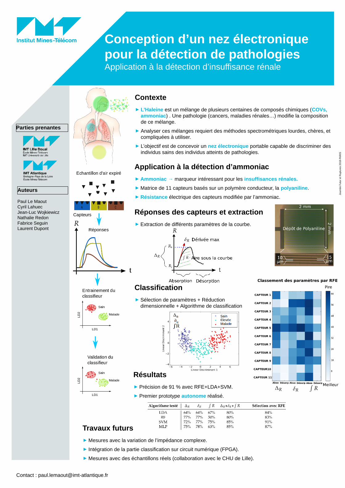
Contexte

► L’Haleine est un mélange de plusieurs centaines de composés chimiques (COVs, ammoniac) . Une pathologie (cancers, maladies rénales…) modifie la composition de ce mélange.

► Analyser ces mélanges requiert des méthodes spectrométriques lourdes, chères, et compliquées à utiliser.

► L’objectif est de concevoir un nez électronique portable capable de discriminer des individus sains des individus atteints de pathologies.

23/01/2018TITRE DE LA PRÉSENTATION 1

Conception d’un nez électronique pour la détection de pathologies Application à la détection d’insuffisance rénale

Application à la détection d’ammoniac

► Ammoniac → marqueur intéressant pour les insuffisances rénales.

► Matrice de 11 capteurs basés sur un polymère conducteur, la polyaniline.

► Résistance électrique des capteurs modifiée par l’ammoniac.

Résultats

► Précision de 91 % avec RFE+LDA+SVM.

► Premier prototype autonome réalisé.

Parties prenantes

Auteurs


Jour

née

Fut

ur e

t R

upt

ure

s 2

018

-PA

RIS

Paul Le MaoutCyril LahuecJean-Luc WojkiewiczNathalie RedonFabrice SeguinLaurent Dupont

Travaux futurs

► Mesures avec la variation de l’impédance complexe.

► Intégration de la partie classification sur circuit numérique (FPGA).

► Mesures avec des échantillons réels (collaboration avec le CHU de Lille).

Réponses des capteurs et extraction

► Extraction de différents paramètres de la courbe.

Classification

► Sélection de paramètres + Réduction dimensionnelle + Algorithme de classification

01/24/2018TITRE DE LA PRÉSENTATION 1

Emergence of Long Term Associative Memories in Recurrent Hebbian Networks Under Noise

A recurrent clustered neural network model

Network Model► Consolidated Hebbian Learning – The activation function of neurons

is chosen so that there are two fixed attractive points: 0 and 1.

► Network Equations – Network equations update at each iteration weigths and activations.

► Properties of the Network – Locality, boundedness, long-term stability, synaptic depression, incremental learning and competition.

Emergence of long term memory

Simulations and Results► Neural Clique Networks – Neural clique networks are autoassociative binary

memories built upon clustered neural networks.

► Performance – They are able to store then reliably retrieve a lot of messages from noisy inputs, providing density of the network remains small.

► Emergence of Neural Clique Networks – We observe that our model is able to make neural clique networks stand out, providing we present each message to store onto the network long enough (number of iterations n

it is

large enough).

Parties prenantes

Auteurs

Partenaires

Contact: [email protected]

Février 2017

Éliott CoyacVincent GriponCharlotte LanglaisClaude Berrou

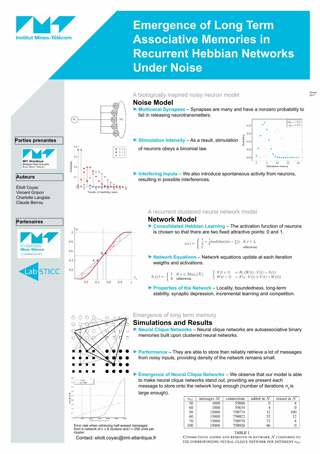
A biologically inspired noisy neuron model

Noise Model► Multicanal Synapses – Synapses are many and have a nonzero probability to

fail in releasing neurotransmetters.

► Stimulation Intensity – As a result, stimulation

of neurons obeys a binomial law.

► Interfering Inputs – We also introduce spontaneous activity from neurons, resulting in possible interferences.

Error rate when retrieving half-erased messages from a network of c = 8 clusters and l = 256 units per cluster.

Understanding the affective

and stylistic human motionFrom the definition of style to its recognition

Stakeholders

Authors

Partners


Fe

bru

ary

20

18

-

Jo

urn

ée

re

stitu

tio

n th

èse

s F

utu

r &

Ru

ptu

res E

ditio

n 2

01

8

• Sarah Ribet

• Hazem Wannous

• Jean-Philippe

Vandeborre

State of the art and contributions

Style in human body motion

Classification of style when seen as individual-related features

Spatio-temporal variations of a motion that add value to the motion, depending on individuals

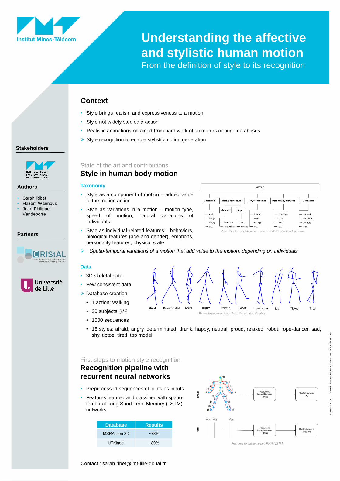
Data

• 3D skeletal data

• Few consistent data

Database creation

• 1 action: walking

• 20 subjects ♂/♀

• 1500 sequences

• 15 styles: afraid, angry, determinated, drunk, happy, neutral, proud, relaxed, robot, rope-dancer, sad,

shy, tiptoe, tired, top model

Example postures taken from the created database

First steps to motion style recognition

Recognition pipeline with

recurrent neural networks

• Preprocessed sequences of joints as inputs

• Features learned and classified with spatio-

temporal Long Short Term Memory (LSTM)

networks

Features extraction using RNN (LSTM)

Taxonomy

• Style as a component of motion – added value

to the motion action

• Style as variations in a motion – motion type,

speed of motion, natural variations of

individuals

• Style as individual-related features – behaviors,

biological features (age and gender), emotions,

personality features, physical state

Context

• Style brings realism and expressiveness to a motion

• Style not widely studied ≠ action

• Realistic animations obtained from hard work of animators or huge databases

Style recognition to enable stylistic motion generation

Database Results

MSRAction 3D ~78%

UTKinect ~89%

Système de Localisation 3D Indoor par

Radar Multistatique UWB

Parties prenantes

Auteurs

Partenaires


Fé

vri

er

20

18

C

ollo

qu

e d

e l’In

stitu

t M

ine

s T

élé

co

m

P

ari

s

Nour Awarkeh

Nel Samama

Jean Christophe-Cousin

Muriel Muller

Contexte et Motivations

Validation du Modèle

Modèle de Localisation Indoor

Mauvaise pénétration des signaux GPS à l’intérieur

des bâtiments

Nécessité des informations de localisation pour de

nombreuses applications

Demande croissante d'exactitude dans les systèmes

de localisation

Résolution temporelle très fine du signal UWB

Nécessité de réaliser un système de Localisation 3D

Indoor en utilisant la technologie UWB

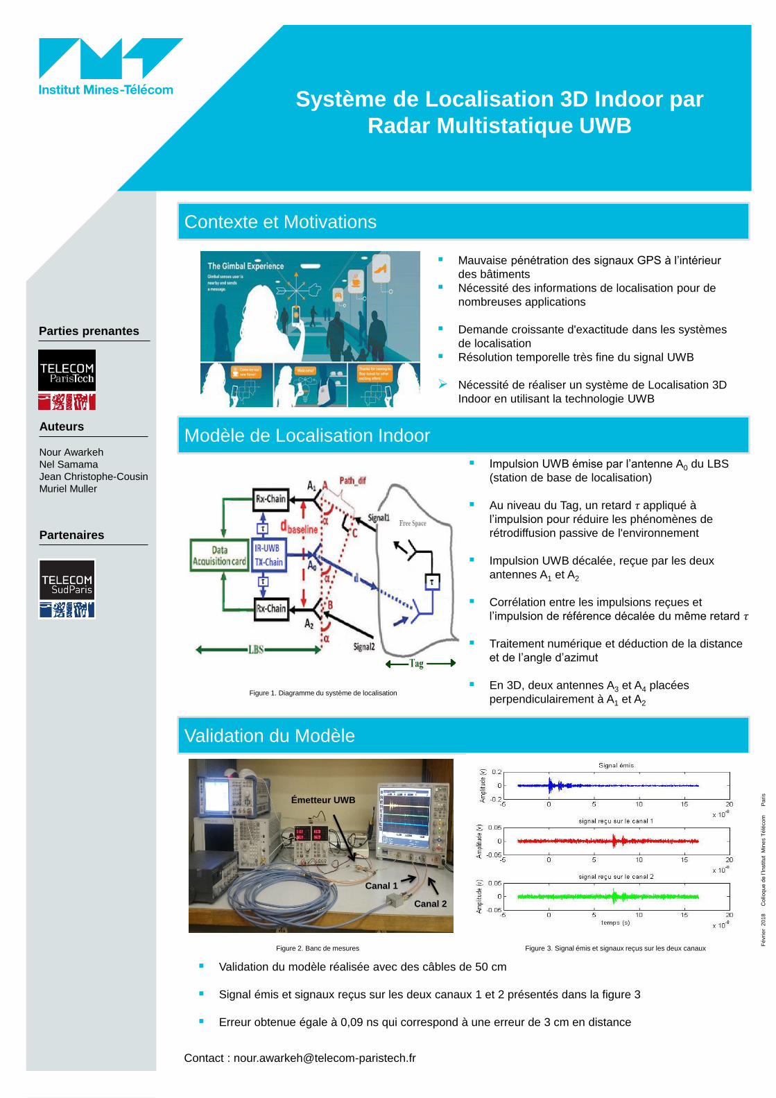
Impulsion UWB émise par l’antenne A0 du LBS

(station de base de localisation)

Au niveau du Tag, un retard 𝜏 appliqué à

l’impulsion pour réduire les phénomènes de

rétrodiffusion passive de l'environnement

Impulsion UWB décalée, reçue par les deux

antennes A1 et A2

Corrélation entre les impulsions reçues et

l’impulsion de référence décalée du même retard 𝜏

Traitement numérique et déduction de la distance

et de l’angle d’azimut

En 3D, deux antennes A3 et A4 placées

perpendiculairement à A1 et A2

Validation du modèle réalisée avec des câbles de 50 cm

Signal émis et signaux reçus sur les deux canaux 1 et 2 présentés dans la figure 3

Erreur obtenue égale à 0,09 ns qui correspond à une erreur de 3 cm en distance

Figure 1. Diagramme du système de localisation

Figure 2. Banc de mesures Figure 3. Signal émis et signaux reçus sur les deux canaux

Émetteur UWB

Canal 1

Canal 2

Cooperation in Cellular Networks.

►Dynamic clusters – The user chooses the group of Base Stations (BS) for

its service. Problems: Intensive communication between the BSs, resource

sharing.

►Static Clusters – The cooperative clusters do not change over time.

Problems: The proposed methodologies produce high interference.

►Static Clusters and proximity – The static clusters are formed by means of

proximity between the nodes: Random Geometric Graph, Lillypond Model,

Nearest Neighbour Model (NNM).

►Mutually Nearest Neighbours (MNN) – Each one of the NN-clusters have

only one of these, for which their cooperation is optimal w.r.t. proximity.

►Modified NNM – The NN-clusters are recovered, iteratively, from the root.

30/11/2017 TITRE DE LA PRÉSENTATION 1

Cooperative Communications in

very large cellular Networks. Nearest Neighbour Cooperation

Properties of the MNNs

When the BSs follow a Poisson Point Process (PPP):

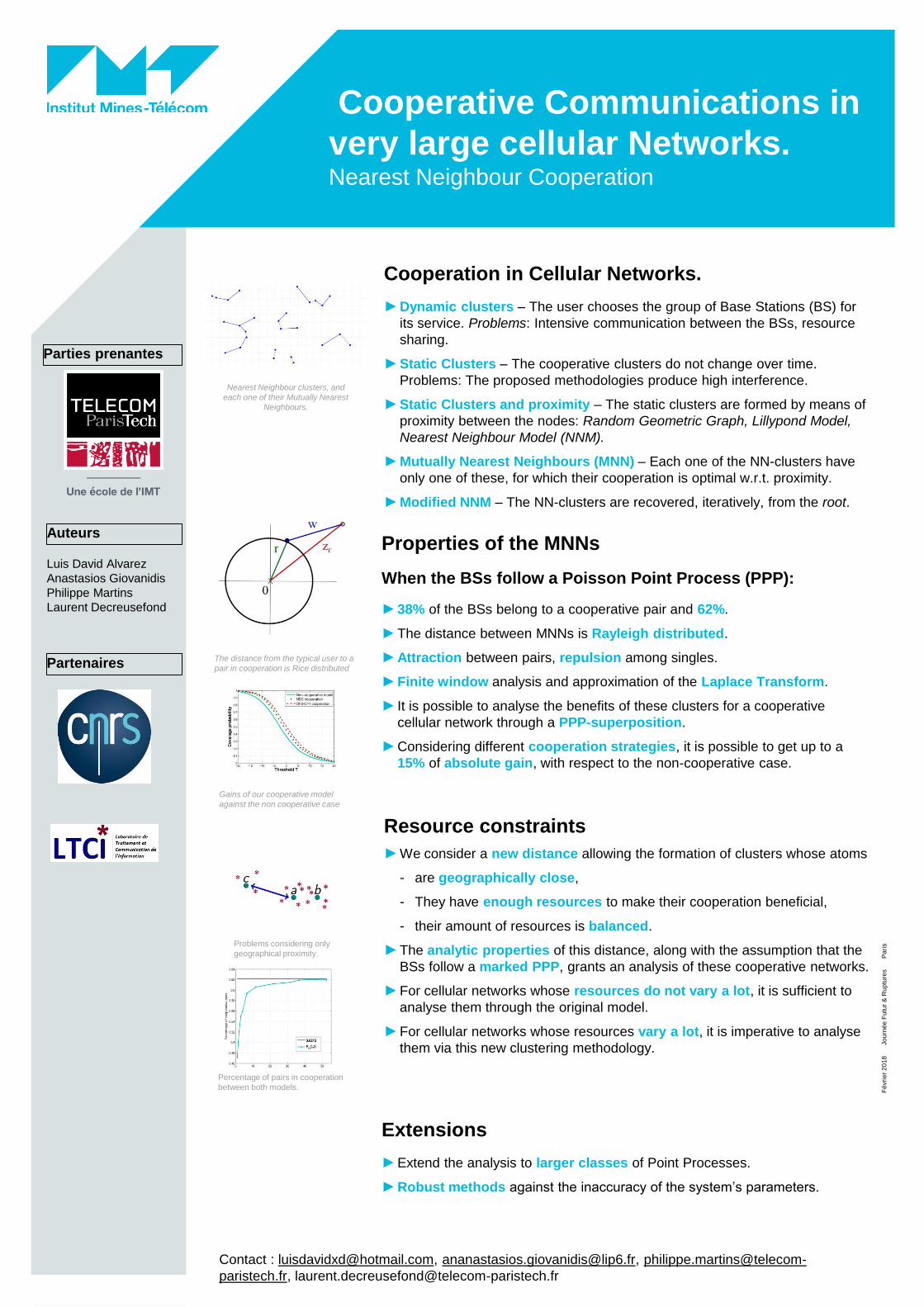
►38% of the BSs belong to a cooperative pair and 62%.

►The distance between MNNs is Rayleigh distributed.

►Attraction between pairs, repulsion among singles.

►Finite window analysis and approximation of the Laplace Transform.

► It is possible to analyse the benefits of these clusters for a cooperative

cellular network through a PPP-superposition.

►Considering different cooperation strategies, it is possible to get up to a

15% of absolute gain, with respect to the non-cooperative case.

Resource constraints

►We consider a new distance allowing the formation of clusters whose atoms

- are geographically close,

- They have enough resources to make their cooperation beneficial,

- their amount of resources is balanced.

►The analytic properties of this distance, along with the assumption that the

BSs follow a marked PPP, grants an analysis of these cooperative networks.

►For cellular networks whose resources do not vary a lot, it is sufficient to

analyse them through the original model.

►For cellular networks whose resources vary a lot, it is imperative to analyse

them via this new clustering methodology.

Parties prenantes

Auteurs

Partenaires

Nearest Neighbour clusters, and

each one of their Mutually Nearest

Neighbours.

The distance from the typical user to a

pair in cooperation is Rice distributed

Problems considering only

geographical proximity.

Contact : [email protected], [email protected], philippe.martins@telecom-

paristech.fr, [email protected]

Fé

vri

er

20

18

Jo

urn

ée

Fu

tur

& R

up

ture

s

P

ari

s

Luis David Alvarez

Anastasios Giovanidis

Philippe Martins

Laurent Decreusefond

Gains of our cooperative model

against the non cooperative case

Percentage of pairs in cooperation

between both models.

Extensions

►Extend the analysis to larger classes of Point Processes.

►Robust methods against the inaccuracy of the system’s parameters.

mailto:[email protected]





TITRE DE LA PRÉSENTATION30/11/2017 1

Gestion de ressources photoniques pour l’application aux réseaux de

communications quantique

Source continue avec un guide d’one AlGaAs [2]

Parties prenantes

Auteurs

Partenaires


Julien Trapateau Eleni Diamanti Isabelle Zaquine

Protocole BBM92 QKD:

❶ choix de base & mesure → Rraw

❷ réconciliation des bases → Rsift

= ½Rraw

❸ estimation de l'erreur & correction → e, f(e)❹ extraction de la clé secrète → R

key

TE00

n

ω

TM00

TEBragg

ωp

ωA

0ω

B

½ωp

1

Résultats Perspectives

ωA

ωB

Distribution de clés quantiques multi-utilisateurs avec uneDistribution de clés quantiques multi-utilisateurs avec unesource semi-conductricesource semi-conductrice

C. Autebert1, J. Trapateau2, A. Orieux2, A. Lemaître3, C. Gomez-Carbonell3,E. Diamanti2, I. Zaquine2, and S. Ducci1

1 Laboratoire MPQ, Université Paris Diderot, Sorbonne Paris Cité, CNRS-UMR 7162, Paris, France2 LTCI, CNRS, Télécom ParisTech, Université Paris-Saclay, Paris, France3 Centre de Nanosciences et de Nanotechnologies, CNRS/Université Paris Sud, UMR 9001 Marcoussis, France

Distribution de clés quantiques

Résumé:

AlGaAs 2-photon source

Expérience

Bibliographie

• BB84 [5] → photons unique ou laser atténué H/V

D/A

H

DV

A

0 0 0 1 110

0

|Ψ>AB

Fluorescence paramétrique dans un guide d'onde AlGaAs [3,4]:

❸ conservation d'énergie:ω

A + ω

B = ω

p (with ω

A ≤ ω

B)

❸ accord de phase (modes transverses):n

TE00(ω

A)ω

A + n

TM00(ω

B)ω

B = n

TEBragg(ω

p)ω

p(1)

nTM00

(ωA)ω

A + n

TE00(ω

B)ω

B = n

TEBragg(ω

p)ω

p(2)

λp (nm)

λ A,B

(nm

)λ A

,B (

nm)

λ A,B

(nm

)

intensité (a.u.)

TE00

TM00

|Ψ>A,B

=|HV> + eiφ|VH>

√2TE

00T

M00

TE

Bra

gg État de Bell directementgénéré:

(faible biréfringence → pasbesoin de compensation dewalk-off)

• BBM92 [6] → paires de photons intriqués

25

25

24

26

23

27

22

28

21

29

ITU 100GHz grid:21 ↔ 1560.61 nm22 ↔ 1559.79 nm23 ↔ 1558.98 nm24 ↔ 1558.17 nm25 ↔ 1557.36 nm26 ↔ 1556.55 nm27 ↔ 1555.75 nm28 ↔ 1554.94 nm29 ↔ 1554.13 nm

ωB = ω

p – ω

A

λp = 778.68 nm

≃ 30 nm

modes transverses:

serveurquantique

TE00

TM00

Serveur quantique

Alice 23

CW Ti:salaser

778.68 nm

MasqueHolographique

63x

RefroidisseurPeltier

Guide d'ondeAlGaAs

10x

long-passfilter

collimateurSMF

DWDM

❸ anti-correlation sur une large bande de fréquence❸ dense wavelength division multiplexing (DWDM)⇒ BBM92-QKD multi-utilisateur avec une seule source

A22A21

A24

Contrôleur depolarisation

λ/2 PBS

APD

Compteur decoïncidence

Bob 27Contrôleur depolarisation

λ/2 PBS

APD

B26

B28B29→ 4 paires de canaux/utilisateurs disponibles

Les protocoles de cryptographie quantique basés sur l'utilisation de paires de photons intriqués montrent une meilleure robustesse auxpertes que ceux qui utilisent des photons uniques ou des lasers atténués [1] ils permettent de garantir une sécurité indépendante desappareils (device-independent QKD) [2]. La mise en œuvre pratique de ces protocoles dans les réseaux de télécommunications par fibrenécessite des sources performantes et facilement intégrables.Ici, nous démontrons la distribution de clés secrètes par fibre entre différents utilisateurs avec une source semi-conductrice [3],compatible en pompage électrique [4], sur une distance de 50 km, avec un taux de clés secrètes de 0.21 bits/s et un QBER of 6.9%.

[1] X.F. Ma, C.-H.F. Fung & H.-K. Lo, Phys. Rev. A 76, 012307(2007).[2] S. Pironio et al., New J. Phys. 11, 045021 (2009).[3] C. Autebert et al., Optica 3, 143–146 (2016).[4] F. Boitier et al., Phys. Rev. Lett. 112, 183901 (2014).

|D> = (|H>+ |V>)/√2|A> = (|H> – |V>)/√2

H2(x) = – x.log(x)

– (1–x).log(1–x)

QBER & taux de clés secrètes [1]:

e = ½(1 – V)R

key ≥ R

sift( 1 – f(e)H

2(e) – H

2(e) )

[5] C.H. Bennett & G. Brassard, in Proc. IEEE Int. Conf. on Computers, Systems andSignal Processing 175, 8 (1984).[6] C.H. Bennett, G. Brassard & N.D. Mermin, Phys. Rev. Lett. 68, 557–559 (1992).[7] E. Waks, A. Zeevi & Y. Yamamoto, Phys. Rev. A 65, 052310 (2002).

τhisto

: temps d'intégration

JSI(A,B), fréquence de pompe778.68 nm:

f(e): coefficient decorrection d'erreur(≃ 1.2)

QBER & taux de génération en fonction de ladistance distance:

V =∑C

max – ∑C

min

∑Cmax

+ ∑Cmin Paramètres de fit [7]:

• pertes de la fibre:α = 0.22 dB/km

• efficacité de collection &détection :

ηcol

= 5% & ηdet

= 20%• Probabilité des coups noirs:

d = 4.4×10-6

• erreur sur la polarisation(PMD):

b = 6%

Cfalse

Cmin

• grand taux de clés/longues distances→ R

key ≥ 3 kbit/s à 0 km et distance ≥ 200 km

accessible, en améliorant la compensation PMD etl'efficacité de collection/détection(b ≤ 2, η

col ≥ 20%

and ηdet

≥ 85%), avec une diode laser collimatée etdes détecteurs supraconducteurs .

• grand nombre d'utilisateur→ 20 paires d'utilisateurs, avec des DWDM de 40

canaux pour exploiter les 30 nm de largeur spectraledes photons intriqués.

• pompage électrique [4] → intégration complète,

pas de procédure d'alignement.C

falseC

max

???

TE⇔ H

TM⇔ V

z

|Ψ>AB

= =|HV> – |VH>

√2

|AD> – |DA>

? ??

√2

Rsift

=∑C

max – ∑C

min

τhisto

Rfalse

=∑C

false

τhisto

VisibilitéHistogramme de coïncidence pour A23–B27 sur 50 km:

Taux de coïncidence enbases identiques:

Taux de faussescoïncidences:

Funding:Funding:




= ½Rraw


key

TE00

n

ω

TM00

TEBragg

ωp

ωA

0ω

B

½ωp

1


ωA

ωB





Résumé:


Expérience

Bibliographie


D/A

H

DV

A

0 0 0 1 110

0

|Ψ>AB



A + ω

B = ω

p (with ω

A ≤ ω

B)


TE00(ω

A)ω

A + n

TM00(ω

B)ω

B = n

TEBragg(ω

p)ω

p(1)

nTM00

(ωA)ω

A + n

TE00(ω

B)ω

B = n

TEBragg(ω

p)ω

p(2)

λp (nm)

λ A,B

(nm

)λ A

,B (

nm)

λ A,B

(nm

)

intensité (a.u.)

TE00

TM00

|Ψ>A,B

=|HV> + eiφ|VH>

√2TE

00T

M00

TE

Bra




25

25

24

26

23

27

22

28

21

29


ωB = ω

p – ω

A

λp = 778.68 nm

≃ 30 nm

modes transverses:

serveurquantique

TE00

TM00

Serveur quantique

Alice 23

CW Ti:salaser

778.68 nm

MasqueHolographique

63x


Guide d'ondeAlGaAs

10x

long-passfilter

collimateurSMF

DWDM


A22A21

A24


λ/2 PBS

APD



λ/2 PBS

APD

B26




|D> = (|H>+ |V>)/√2|A> = (|H> – |V>)/√2

H2(x) = – x.log(x)

– (1–x).log(1–x)


e = ½(1 – V)R

key ≥ R

sift( 1 – f(e)H

2(e) – H

2(e) )


τhisto





V =∑C

max – ∑C

min

∑Cmax




ηcol

= 5% & ηdet


d = 4.4×10-6


b = 6%

Cfalse

Cmin




col ≥ 20%

and ηdet






falseC

max

???

TE⇔ H

TM⇔ V

z

|Ψ>AB

= =|HV> – |VH>

√2

|AD> – |DA>

? ??

√2

Rsift

=∑C

max – ∑C

min

τhisto

Rfalse

=∑C

false

τhisto




Funding:Funding:

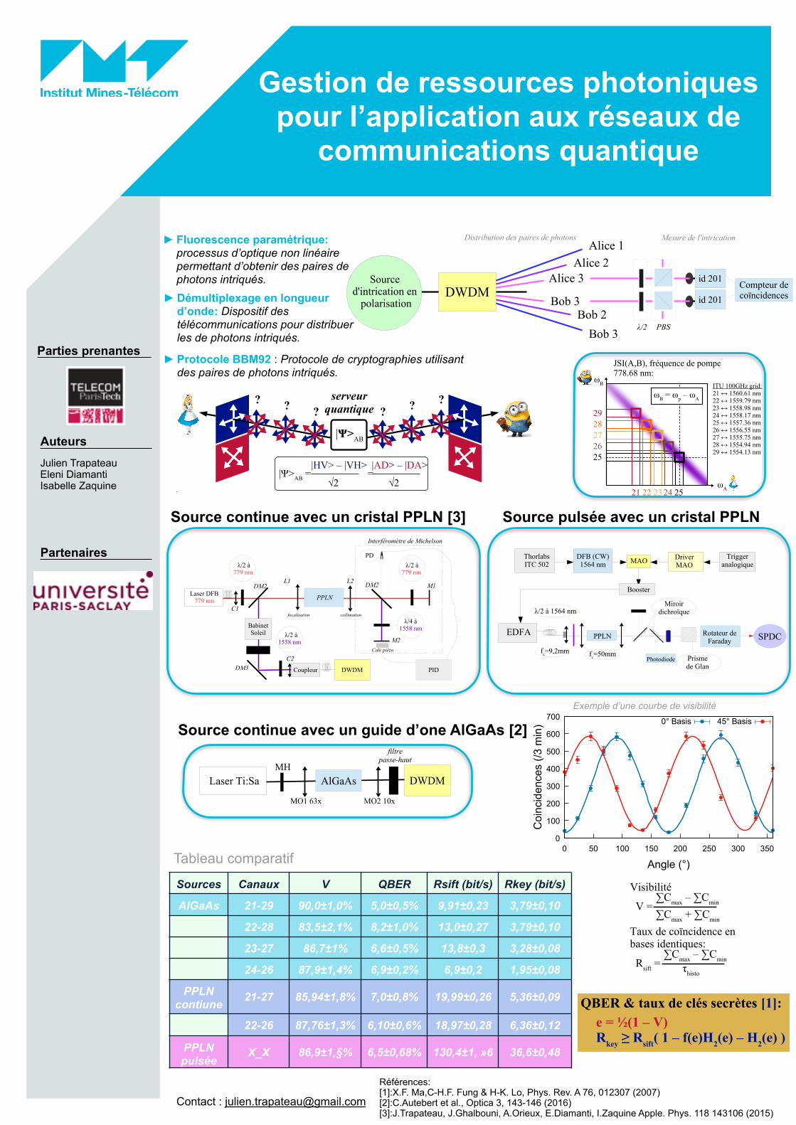
► Protocole BBM92 : Protocole de cryptographies utilisant des paires de photons intriqués.

DWDM

Alice 1

Alice 2

Alice 3

Bob 3Bob 2

Bob 3

Source d'intrication en

polarisation

Distribution des paires de photons Mesure de l'intrication

PBSλ/2

id 201

id 201

Compteur decoïncidences

► Fluorescence paramétrique: processus d’optique non linéaire permettant d’obtenir des paires de photons intriqués.

►Démultiplexage en longueur d’onde: Dispositif des télécommunications pour distribuer les de photons intriqués.

Source continue avec un cristal PPLN [3]

Laser Ti:Sa AlGaAs DWDM

MO1 63x MO2 10x

MH

filtrepasse-haut

Triggeranalogique

ThorlabsITC 502

DFB (CW)1564 nm

DriverMAO

MAO

Booster

EDFA

fc=9,2mm

λ/2 à 1564 nm

Photodiodef

c=50mm

Rotateur deFaraday

SPDC

Miroirdichroïque

Prismede Glan

PPLN

Laser DFB779 nm

BabinetSoleil

Coupleur

Interféromètre de Michelson

focalisation collimation

DM2

DM3

λ/2 à779 nm

λ/4 à1558 nm

M2

M1

PPLN

DM2

λ/2 à779 nm

PD

DWDM

λ/2

Cale piézo

L1 L2

λ/2 à1558 nm

C2

C1

PID

Source pulsée avec un cristal PPLN

Tableau comparatif

Sources Canaux V QBER Rsift (bit/s) Rkey (bit/s)

AlGaAs 21-29 90,0±1,0% 5,0±0,5% 9,91±0,23 3,79±0,10

22-28 83,5±2,1% 8,2±1,0% 13,0±0,27 3,79±0,10

23-27 86,7±1% 6,6±0,5% 13,8±0,3 3,28±0,08

24-26 87,9±1,4% 6,9±0,2% 6,9±0,2 1,95±0,08

PPLN contiune 21-27 85,94±1,8% 7,0±0,8% 19,99±0,26 5,36±0,09

22-26 87,76±1,3% 6,10±0,6% 18,97±0,28 6,36±0,12

PPLN pulsée

X_X 86,9±1,§% 6,5±0,68% 130,4±1, »6 36,6±0,48

Références: [1]:X.F. Ma,C-H.F. Fung & H-K. Lo, Phys. Rev. A 76, 012307 (2007) [2]:C.Autebert et al., Optica 3, 143-146 (2016) [3]:J.Trapateau, J.Ghalbouni, A.Orieux, E.Diamanti, I.Zaquine Apple. Phys. 118 143106 (2015)

Exemple d’une courbe de visibilité




= ½Rraw


key

TE00

n

ω

TM00

TEBragg

ωp

ωA

0ω

B

½ωp

1


ωA

ωB





Résumé:


Expérience

Bibliographie


D/A

H

DV

A

0 0 0 1 110

0

|Ψ>AB



A + ω

B = ω

p (with ω

A ≤ ω

B)


TE00(ω

A)ω

A + n

TM00(ω

B)ω

B = n

TEBragg(ω

p)ω

p(1)

nTM00

(ωA)ω

A + n

TE00(ω

B)ω

B = n

TEBragg(ω

p)ω

p(2)

λp (nm)

λ A,B

(nm

)λ A

,B (

nm)

λ A,B

(nm

)

intensité (a.u.)

TE00

TM00

|Ψ>A,B

=|HV> + eiφ|VH>

√2TE

00T

M00

TE

Bra




25

25

24

26

23

27

22

28

21

29


ωB = ω

p – ω

A

λp = 778.68 nm

≃ 30 nm

modes transverses:

serveurquantique

TE00

TM00

Serveur quantique

Alice 23

CW Ti:salaser

778.68 nm

MasqueHolographique

63x


Guide d'ondeAlGaAs

10x

long-passfilter

collimateurSMF

DWDM


A22A21

A24


λ/2 PBS

APD



λ/2 PBS

APD

B26




|D> = (|H>+ |V>)/√2|A> = (|H> – |V>)/√2

H2(x) = – x.log(x)

– (1–x).log(1–x)


e = ½(1 – V)R

key ≥ R

sift( 1 – f(e)H

2(e) – H

2(e) )


τhisto





V =∑C

max – ∑C

min

∑Cmax




ηcol

= 5% & ηdet


d = 4.4×10-6


b = 6%

Cfalse

Cmin




col ≥ 20%

and ηdet






falseC

max

???

TE⇔ H

TM⇔ V

z

|Ψ>AB

= =|HV> – |VH>

√2

|AD> – |DA>

? ??

√2

Rsift

=∑C

max – ∑C

min

τhisto

Rfalse

=∑C

false

τhisto




Funding:Funding:




= ½Rraw


key

TE00

n

ω

TM00

TEBragg

ωp

ωA

0ω

B

½ωp

1


ωA

ωB





Résumé:


Expérience

Bibliographie


D/A

H

DV

A

0 0 0 1 110

0

|Ψ>AB



A + ω

B = ω

p (with ω

A ≤ ω

B)


TE00(ω

A)ω

A + n

TM00(ω

B)ω

B = n

TEBragg(ω

p)ω

p(1)

nTM00

(ωA)ω

A + n

TE00(ω

B)ω

B = n

TEBragg(ω

p)ω

p(2)

λp (nm)

λ A,B

(nm

)λ A

,B (

nm)

λ A,B

(nm

)

intensité (a.u.)

TE00

TM00

|Ψ>A,B

=|HV> + eiφ|VH>

√2TE

00T

M00

TE

Bra




25

25

24

26

23

27

22

28

21

29


ωB = ω

p – ω

A

λp = 778.68 nm

≃ 30 nm

modes transverses:

serveurquantique

TE00

TM00

Serveur quantique

Alice 23

CW Ti:salaser

778.68 nm

MasqueHolographique

63x


Guide d'ondeAlGaAs

10x

long-passfilter

collimateurSMF

DWDM


A22A21

A24


λ/2 PBS

APD



λ/2 PBS

APD

B26




|D> = (|H>+ |V>)/√2|A> = (|H> – |V>)/√2

H2(x) = – x.log(x)

– (1–x).log(1–x)


e = ½(1 – V)R

key ≥ R

sift( 1 – f(e)H

2(e) – H

2(e) )


τhisto





V =∑C

max – ∑C

min

∑Cmax




ηcol

= 5% & ηdet


d = 4.4×10-6


b = 6%

Cfalse

Cmin




col ≥ 20%

and ηdet






falseC

max

???

TE⇔ H

TM⇔ V

z

|Ψ>AB

= =|HV> – |VH>

√2

|AD> – |DA>

? ??

√2

Rsift

=∑C

max – ∑C

min

τhisto

Rfalse

=∑C

false

τhisto




Funding:Funding:

6.3. RESULTS 83

6.3 Results

Zero distance between Alice and Bob

QKD experiments were first performed with the entangled photons entering directly the stationsof Alice and Bob, for all four symmetric channel pairs (21-29; 22-28; 23-27; 24-26) of the DWDM,corresponding to four di�erent pairs of users sharing a secret key.

0

100

200

300

400

500

600

700

0 50 100 150 200 250 300 350

Coi

ncid

ence

s (/3

min

)

Angle (°)

0° Basis 45° Basis

Figure 6.3 – Visibility curve in the natural and diagonal polarization basis for ITU channel pair23-27.

Figure 6.3 displays the complete visibility curves for the 23-27 channel pair when the Alicemeasurement basis is set to the natural (0¶) or diagonal (45¶) basis, and the Bob measurement basisvaries. Figure 6.4 shows the measured coincidence histograms corresponding to the eight possibleprojective measurements obtained when Alice and Bob make the same basis choice, also for the23-27 channel pair. From these measurements, it is possible in all cases to estimate the sifted keygeneration rate, Rsift = 1

2Rraw, by calculating from the obtained data:

Rsift =CHH

p + CHVp + CV V

p + CV Hp + CDD

p + CDAp + CAA

p + CADp

·, (6.6)

in which each of the eight terms is obtained by adding together the number of coincidences measuredin the five bins corresponding to the coincidence peak in figure 6.4 accumulated over a time · = 3 min.

It is also possible to calculate the false coincidence rate as:

Rfalse = 2CHH0 + CHV

0 + CV V0 + CV H

0 + CDD0 + CDA

0 + CAA0 + CAD

0·

, (6.7)

in which each of the terms is obtained from the mean value of the number of coincidences measuredin five bins outside the coincidence peak.

Finally, the maximum and minimum number of coincidences in both bases are given by:Y]

[Cmax = CHV

p + CV Hp + CDD

p + CAAp

Cmin = CHHp + CV V

p + CDAp + CAD

p .

(6.8a)(6.8b)

These are inserted in eq. 6.4 to calculate the total entanglement visibility Vtot, which leads tothe calculation of the QBER (eq. 6.3). Finally, taking standard values for f(e) [147, 149], eq. 6.5


Trust based secure routing

for the Internet of Things.

►The Internet of Things (IoT) objects typically

collect, communicate and share data that can be

used to derive sensitive information and to make

decentralized decisions.

►Data packets are transmitted, collected and

distributed via RPL, the routing protocol for Low

power and Lossy networks considered as the

standard protocol of IoT.

Parties prenantes

Auteurs

Partenaires


Fé

vri

er

20

18

F

utu

r &

Ru

ptu

res M

ine

s T

élé

co

m

P

ari

s

Asma LAHBIB

Context Problematic

RPL network is composed of embedded

devices with limited power, memory, and

processing resources thus their overuse in

routing may lead to battery depletion

The RPL protocol is exposed to a large

variety of security attacks causing the loss of

a large part of the traffic.

Participating entities may change their

behavior which could disturb the

network functioning.

►How to extend the battery life of IoT objects?

►How to be sure that the data received are not

corrupted by some malicious nodes in the network?

►How to trust the participating network nodes and

how to trust the route data was transmitted over?

Proposed approach

Enhancing the security aspect of RPL routing protocol.

Ensuring Trust among entities by considering Trust

related to their forwarding behavior as well as that related

to the quality of the connecting link.

Trust computation is based on a set of properties including

the reputation parameters, the energy considerations

and the QoS factors.

Integration of the proposed model into the RPL DODAG

construction and maintenance phases, Trust values are

used for rank computation and thus for preferred parent

selection.

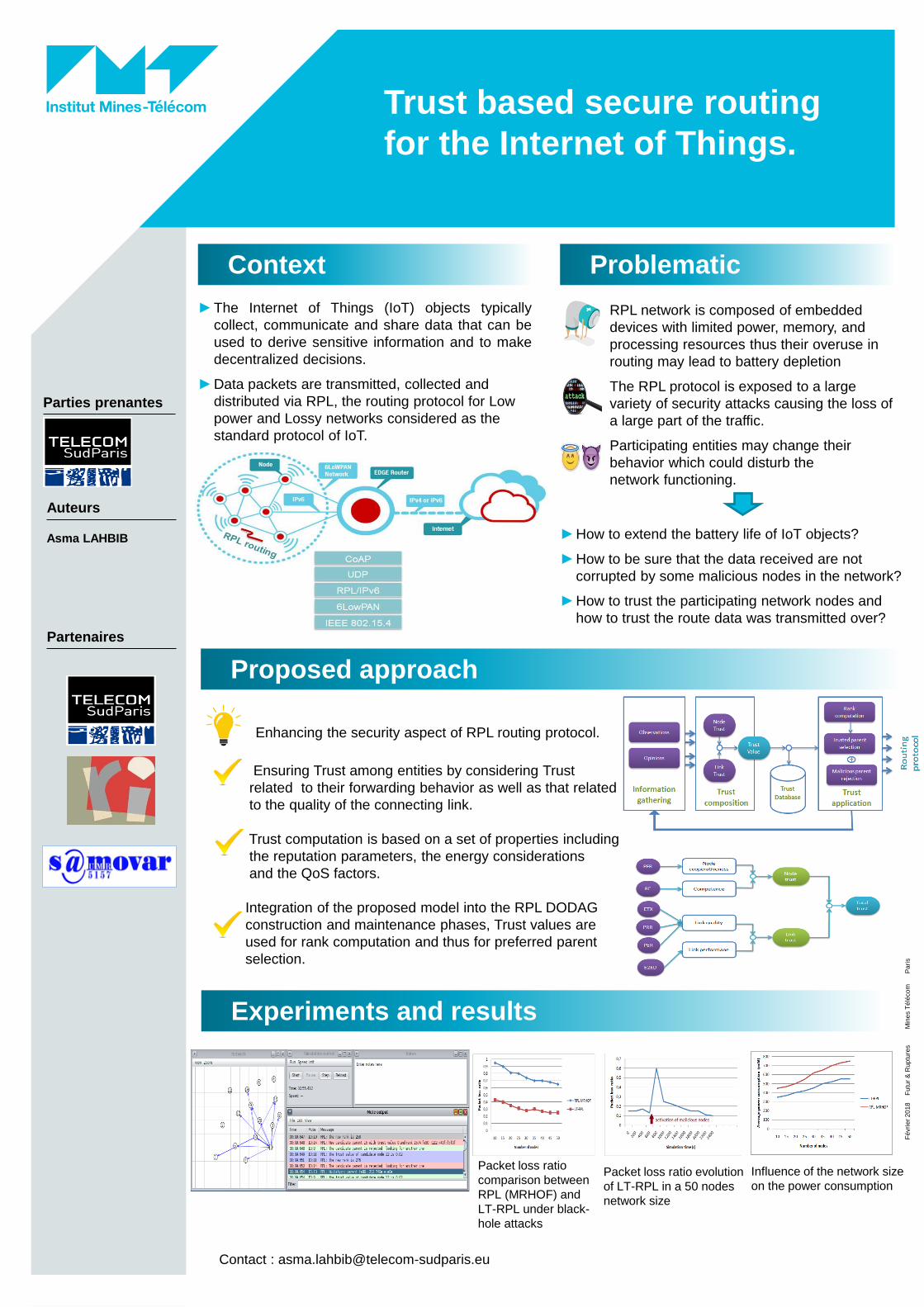
Experiments and results

Packet loss ratio evolution

of LT-RPL in a 50 nodes

network size

Influence of the network size

on the power consumption

Packet loss ratio

comparison between

RPL (MRHOF) and

LT-RPL under black-

hole attacks

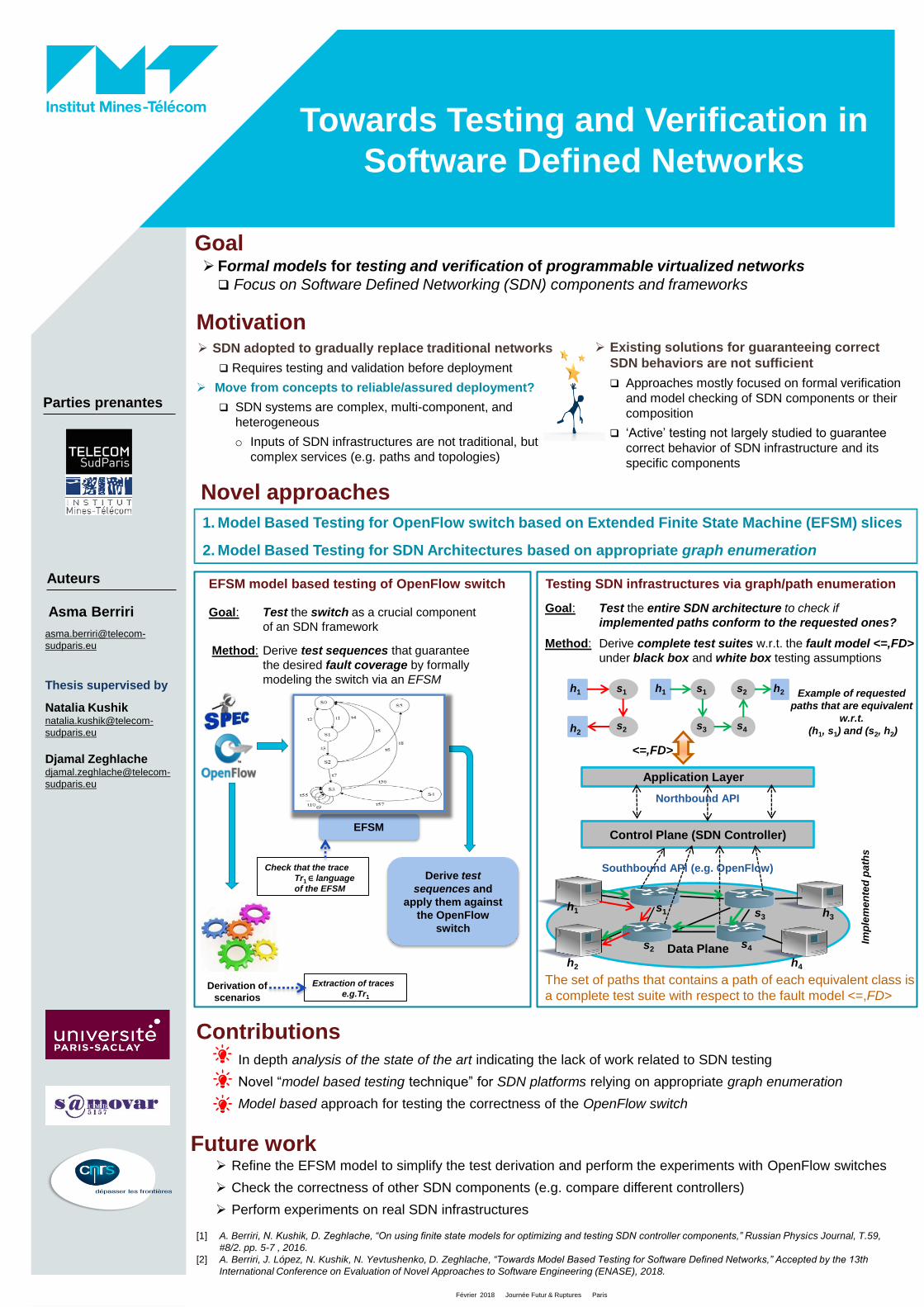
Goal

Towards Testing and Verification in

Software Defined Networks

Novel approaches

In depth analysis of the state of the art indicating the lack of work related to SDN testing

Novel “model based testing technique” for SDN platforms relying on appropriate graph enumeration

Model based approach for testing the correctness of the OpenFlow switch

Parties prenantes

Auteurs

Février 2018 Journée Futur & Ruptures Paris

Asma Berriri

asma.berriri@telecom-

sudparis.eu

Thesis supervised by

Natalia Kushik natalia.kushik@telecom-

sudparis.eu

Djamal Zeghlache djamal.zeghlache@telecom-

sudparis.eu

Testing SDN infrastructures via graph/path enumeration

Goal: Test the entire SDN architecture to check if

implemented paths conform to the requested ones?

Method: Derive complete test suites w.r.t. the fault model <=,FD>

under black box and white box testing assumptions

Refine the EFSM model to simplify the test derivation and perform the experiments with OpenFlow switches

Check the correctness of other SDN components (e.g. compare different controllers)

Perform experiments on real SDN infrastructures

[1] A. Berriri, N. Kushik, D. Zeghlache, “On using finite state models for optimizing and testing SDN controller components,” Russian Physics Journal, T.59,

#8/2. pp. 5-7 , 2016.

[2] A. Berriri, J. López, N. Kushik, N. Yevtushenko, D. Zeghlache, “Towards Model Based Testing for Software Defined Networks,” Accepted by the 13th

International Conference on Evaluation of Novel Approaches to Software Engineering (ENASE), 2018.

Motivation SDN adopted to gradually replace traditional networks

Requires testing and validation before deployment

Move from concepts to reliable/assured deployment?

SDN systems are complex, multi-component, and

heterogeneous

o Inputs of SDN infrastructures are not traditional, but

complex services (e.g. paths and topologies)

1. Model Based Testing for OpenFlow switch based on Extended Finite State Machine (EFSM) slices

2. Model Based Testing for SDN Architectures based on appropriate graph enumeration

EFSM model based testing of OpenFlow switch

Goal: Test the switch as a crucial component

of an SDN framework

Method: Derive test sequences that guarantee

the desired fault coverage by formally

modeling the switch via an EFSM

Derivation of

scenarios

EFSM

Check that the trace

Tr1 ∈ language

of the EFSM

Extraction of traces

e.g.Tr1

Derive test

sequences and

apply them against

the OpenFlow

switch

Formal models for testing and verification of programmable virtualized networks

Focus on Software Defined Networking (SDN) components and frameworks

Contributions

Future work

Imp

lem

en

ted

path

s

The set of paths that contains a path of each equivalent class is

a complete test suite with respect to the fault model <=,FD>

Example of requested

paths that are equivalent

w.r.t.

(h1, s1) and (s2, h2)

h1 h2 s2

s3 s4

s1 h1

h2

s1

s2

<=,FD>

Existing solutions for guaranteeing correct

SDN behaviors are not sufficient

Approaches mostly focused on formal verification

and model checking of SDN components or their

composition

‘Active’ testing not largely studied to guarantee

correct behavior of SDN infrastructure and its

specific components

Data Plane

s1 s3

s4 s2

Control Plane (SDN Controller)

h1

h2

h3

h4

Northbound API

Southbound API (e.g. OpenFlow)

Application Layer












Methodology of data collection:

► First, we download information about apps on the

Google PlayStore. We use python to scrap apps from

the Google PlayStore.

► We improve the database by collecting publicly

available data on Privacy Grade.

► Privacy Grade is an ongoing project of a group of

computer science researchers at Carnegie Mellon

University.

- They measure the gap between users’ expectations

about an app’s behavior and the app’s actual

behavior in terms of privacy.

Personal data and regulation Empirical and experimental approach

Stakeholder

Authors

Key figures

Python and Android logo

Distribution of top third parties


Website: https://sites.google.com/view/vincentlefrere/accueil

15

Fé

vri

er

20

18

Jo

urn

ée

Fu

tur

& R

up

ture

s, I

nstitu

t M

ine

s T

ele

co

m

Vincent Lefrere Grazia Cecere Fabrice Le Guel

Playstore in 2015:

• 1,292,029 free

apps

• 85% apps are free

Our Sample:

• 475 867 free apps

• data on privacy

• Data about thirds

parties

Descriptive results:

• Admob (Google)

86% of market

share

Our results:

• Killer apps

requested more

personal data

• Advertising is for

small developers

• Integrated

purchase is

substitute to the

collect of personal

data

Strategy of monetization by downloads

Main Objectives:

► Investigate the market of personal data through

the market of smartphone application

► Improve the understanding of the free digital

goods

► Explore the market of smartphone

applications

► Identify the different strategies of monetization

according the characteristics of the apps

► Analyze the market of thirds parties (libraries)

Conclusion

► Platform can improve transparency in forcing

applications to declare the thirds parties to end

users

► Within advertising thirds parties, Admob (Google)

is the major actor of smartphone application

► There is a link between thirds parties and

personal data

► "Big apps" use more personal data compared to

the less downloaded apps

Research questions and literature:

► In the market for smartphone applications, the

majority of apps are zero priced.

► Developers have to monetize theirs apps

► However little is known about their monetization

strategies.

► We contribute to three literature strands:

- Economics of free digital goods

- Economics of mobile applications

- Economics of privacy

Estimation: Recursive Trivariate probit




https://sites.google.com/view/vincentlefrere/accueil

https://sites.google.com/view/vincentlefrere/accueil

journée restitution des travaux de thèses du programme ... · une pathologie (cancers, maladies...

Documents