Journal of Hydrology 452–453 (2012) 259–281

Contents lists available at SciVerse ScienceDirect

Journal of Hydrology

journal homepage: www.elsevier .com/ locate / jhydrol

Trends in precipitation and temperature in Florida, USA

Christopher J. Martinez ⇑, Jerome J. Maleski, Martin F. MillerDepartment of Agricultural and Biological Engineering, Institute of Food and Agricultural Sciences, University of Florida, Gainesville, FL, USA

a r t i c l e i n f o s u m m a r y

Article history:Received 27 September 2011Received in revised form 21 May 2012Accepted 29 May 2012Available online 7 June 2012This manuscript was handled by AndrasBardossy, Editor-in-Chief, with theassistance of Efrat Morin, Associate Editor

Keywords:TrendPrecipitationTemperature

0022-1694/$ - see front matter � 2012 Elsevier B.V. Ahttp://dx.doi.org/10.1016/j.jhydrol.2012.05.066

⇑ Corresponding author. Address: PO Box 110570Tel.: +1 352 392 1864x279.

E-mail address: chrisjm@ufl.edu (C.J. Martinez).

Annual, seasonal, and monthly trends in precipitation, mean temperature, maximum temperature, min-imum temperature, and temperature range were evaluated using stations from the United States Histor-ical Climatology Network (USHCN) for the time periods 1895–2009 and 1970–2009 for the state ofFlorida. The significance and magnitude of station trends were determined using the non-parametricMann–Kendall test and Sen’s slope, respectively. The collective, field significance of trends were evalu-ated using a Monte Carlo permutation procedure. Field significant trends in seasonal precipitation werefound in only the June–August and March–May seasons for the 1895–2009 and 1970–2009 time periods,respectively. Significant decreasing trends in monthly precipitation were found in the months of Octoberand May for the 1895–2009 and 1970–2009 time periods, respectively. Field significant trends werefound for all temperature variables for both time periods, with the largest number of stations with sig-nificant trends occurring in the summer and autumn months. Trends in mean, maximum, and minimumtemperature were generally positive with a higher proportion of positive trends in the 1970–2009 period.The spatial coherence of trends in temperature range was generally less compared to other temperaturevariables, with a larger proportion of stations showing negative trends in the summer and positive trendsat other times of the year and more negative trends found in the 1970–2009 period. Significant differ-ences in temperature trends based on the surrounding land use were found for minimum temperatureand temperature range in the 1970–2009 period indicating that data homogenization of the USHCN tem-perature data did not fully remove this influence. The evaluation of trends based on station exposure rat-ings show significant differences in temperature variables in both the 1895–2009 and 1970–2009 timeperiods. Systematic changes in trends can be seen in the 1980s, the period of widespread conversion fromliquid-in-glass to electronic measurement, indicating that some of the differences found may be due touncorrected inhomogeneities. Since notable differences were found between differently rated stationspre-1940, a time which the present-day rating should have little to no influence, attribution of differencesbased on station rating should be done with caution.

� 2012 Elsevier B.V. All rights reserved.

1. Introduction

Historical trends in surface climate have received considerableattention in recent years as interest in local and regional scaleadaption and mitigation strategies to potential future changes inclimate has increased, primarily in the area of water resourcemanagement (e.g. Arnell and Delaney, 2006; Barsugli et al., 2009;Hamlet, 2011; Rosenzweig et al., 2007). It has been recognized thatglobal or continental scale observations of historical climate orprojections of future climate are less than useful for local or regio-nal scale planning (Barsugli et al., 2009; Brekke et al., 2009;Raucher, 2011). Thus, the evaluation of historical trends or futureprojections on a regional or local scale is needed.

ll rights reserved.

, Gainesville, FL 32611, USA.

The evaluation of observed long-term trends using the UnitedStates Historical Climatology Network (USHCN) has been compli-cated by inconsistencies in measurement instruments, time ofobservations, and station siting (Hubbard and Lin, 2006; Karl etal., 1986; Karl et al., 1988; Peterson and Owen, 2005). Considerableeffort has been made to correct surface observations for theseinconsistencies; including adjustments for both documented andundocumented discontinuities (Menne and Williams, 2009),adjustments for the time of observation bias (Karl et al., 1986; Voseet al., 2003), and minimizing bias of estimates of missing monthlyvalues using an optimal interpolation approach (Menne et al.,2009). Nevertheless, adjusted observation records should not beconsidered to be completely free from error (Davey and Pielke,2005; Fall et al., 2011; Menne et al., 2010; Pielke et al., 2007).For example, Fall et al. (2011) classified stations from the USHCNusing the more rigorous station siting system of the United StatesClimate Reference Network (USCRN) and found significantdifferences between ‘‘good’’ and ‘‘poorly’’ sited station trends in

260 C.J. Martinez et al. / Journal of Hydrology 452–453 (2012) 259–281

maximum temperature, minimum temperature, and temperaturerange. The adjustments made to correct temperature biases inthe USHCN tended to reduce, but did not eliminate trend differ-ences between good and poorly sited stations. In addition, Fallet al. (2011) found that opposite signed trends in maximum andminimum temperature at poorly sited stations cancel the effecton mean temperature, with mean temperature trends indistin-guishable across station classes, but the opposite signed trendsmagnified differences in temperature range. In a similar studyusing a smaller number of stations and a different grouping of

Table 1Stations from the United States Historical Climatology Network used in this study.

COOP ID Station Lat. Long. CRN classificati

080211 Apalachicola AP 29.73 �85.02 1080228 Arcadia 27.22 �81.87 3080478 Bartow 27.90 �81.84 5080611 Belle Glade 26.69 �80.67 2082220a,b De Funiak Springs 1 30.72 �86.09 3082850 Everglades 25.85 �81.39 4082915 Federal Point 29.76 �81.54 4082944 Fernandina Beach 30.66 �81.46 4083163 Ft. Lauderdale 26.10 �80.20 4083186 Ft. Myers Page Field 26.59 �81.86 1083207 Ft. Pierce 27.46 �80.35 4084289 Inverness 3 SE 28.80 �82.31 4084570a Key West Intl. AP 24.56 �81.75 n/a084731 Lake City 2E 30.19 �82.59 4085275 Madison 30.45 �83.41 4086414 Ocala 29.08 �82.08 n/a086997 Pensacola 30.48 �87.19 1087020a Perrine 4 W 25.58 �80.44 4087851 Saint Leo 28.34 �82.26 4088758 Tallahassee WSO AP 30.39 �84.35 1088824 Tarpon SPGS Sewage PL 28.16 �82.76 4088942 Titusville 28.62 �80.82 5

a Station not included in 1895–2009 precipitation trends due to incomplete data.b Station not included in 1970–2009 precipitation trends due to incomplete data.c Station classification from www.surfacestations.org, accessed 9/2/2011.d Land use within a 10-km radius of station.

Fig. 1. 2006 Land use/land cover from the NLCD dataset. V

‘‘good’’ and ‘‘poor’’ stations, Menne et al. (2010) found that poorsiting typically resulted in an overall cool bias in adjusted maxi-mum temperature.

Recent work has shown that regional land use/land cover canhave impact on observed temperature trends (e.g. Christy et al.,2006; Kalnay and Cai, 2003; Pielke et al., 2007). Gallo et al.(1996) found significantly lower diurnal temperature range at ur-ban stations compared to rural stations and Karl et al. (1988) foundurbanization to increase minimum temperature in all seasons andto decrease maximum temperature in all seasons except winter.

onc Breaks detected Predominant Landused

1904, 2007 Open water, WetlandsWetlands, Pasture, Crops

1963 Wetlands, Residential/Urban, Grassland1973 Crops

Forest, Shrub/Scrub, Residential/UrbanWetlands, Open water

1919, 1920, 1995, 1998 Wetlands, Open water, CropsOpen water, Wetlands, Residential/UrbanResidential/Urban

1963 Residential/Urban, WetlandsResidential/Urban, Wetlands, Open water

2004, 2005 Wetlands, Residential/Urban, ForestOpen water, wetlands

1964, 2004, 2009 Forest, Wetlands, Residential/Urban1904, 1953, 1968 Forest, Wetlands, Shrub/Scrub1982 Residential/Urban, Pasture, Forest1906, 2007 Residential/Urban, Open water

Residential/Urban, CropsWetlands, Pasture, Residential/Urban

1962, 1981 Residential/Urban, Forest, WetlandsResidential/Urban, Open waterWetlands, Open water

alues next to stations indicate the CRN classification.

C.J. Martinez et al. / Journal of Hydrology 452–453 (2012) 259–281 261

However, a recent study by Mishra and Lettenmaier (2011) sug-gested that much of the temperature related trends were attribut-able to regional changes in climate rather than to local effects ofurbanization. Land cover type has been shown to influence surfacemoisture content which can then affect temperature (Fall et al.,2010a; Peterson et al., 2011). The conversion of land to irrigatedagriculture has been reported to decrease surface temperature (Fallet al., 2010b; Lobell and Bonfils, 2008; Mahmood et al., 2006; Royet al., 2007). Marshall et al. (2004a, 2004b) found that the large-scale drainage of wetlands and conversion to agriculture in south-ern Florida was associated with increased July–August maximumtemperature and increased incidence of winter killing freezes.The increase of surface moisture due to irrigation or inundation re-sults in an increased partition of available energy to latent heat,reducing sensible heat and cooling of the land surface (NRC,2005). In addition, the increased thermal inertia of wet soil orstanding water increases surface humidity, resulting in an increasein surface heat storage and an increase in surface minimum tem-perature (Marshall et al., 2004b).

In light of both the recent interest in local/regional historicaltrends in surface climate and the concern on the potential biasesin the climate record, the evaluation of trends as conducted in thisstudy may thus serve two purposes: (1) to document the existenceand collective significance of long-term and recent trends in theobserved climate record in Florida and (2) to provide a first stepin further analyses of potential offending stations since the influ-ence of non-standard station siting or land cover conversion canonly be determined by analysis of station data (Menne et al.,2010).

2. Data

Monthly precipitation, mean temperature, maximum tempera-ture and minimum temperature were obtained for 22 stations in

Table 2Number of stations with significant trends in non-homogenized precipitation at p < 0.05.followed by ⁄ are field significant.

Mann–Kendall

1895–2009 1970–2009

+ � + �

Annual 2 (5⁄) 1 (2⁄) 1 (1) 1 (1)

Season + � + �JFM 0 (1) 0 (0) 0 (0) 2 (4)FMA 1 (1) 0 (0) 0 (1) 0 (0)MAM 0 (0) 0 (1) 0 (0) 4 (7⁄)AMJ 0 (1) 1 (1) 0 (0) 0 (0)MJJ 1 (2) 0 (1) 0 (0) 0 (1)JJA 3⁄ (4⁄) 1⁄ (3⁄) 1 (2) 0 (0)JAS 2 (3⁄) 2 (2⁄) 1 (2) 0 (0)ASO 0 (0) 1 (2) 3 (5) 0 (0)SON 1 (1) 0 (0) 1 (1) 0 (0)OND 1 (1) 1 (1) 2 (2) 0 (0)NDJ 1 (2) 0 (0) 0 (0) 3 (5)DJF 0 (0) 0 (0) 0 (0) 3 (3)

Month + � + �Jan 2 (3) 0 (0) 0 (0) 1 (2)Feb 0 (0) 0 (0) 0 (0) 3 (4)Mar 1 (4) 0 (0) 0 (0) 0 (0)Apr 0 (1) 0 (1) 2 (3) 0 (0)May 0 (0) 4 (7⁄) 0 (0) 9⁄ (15June 2 (2) 0 (1) 0 (1) 0 (0)July 1 (1) 1 (3) 1 (1) 0 (0)Aug 2 (3) 1 (1) 0 (0) 0 (0)Sept 0 (0) 0 (0) 1 (2) 0 (0)Oct 0 (0) 6⁄ (7⁄) 0 (0) 0 (0)Nov 2 (2) 0 (0) 0 (0) 0 (1)Dec 0 (0) 0 (0) 0 (0) 0 (0)

Florida for the period 1895–2009 from the USHCN Version 2 SerialMonthly Dataset (Menne et al., 2009; Menne and Williams, 2011)from the Carbon Dioxide Information Analysis Center (http://cdi-ac.ornl.gov/epubs/ndp/ushcn/ushcn.html) (Table 1 and Fig. 1). TheUSHCN contains Cooperative Network (COOP) stations selectedbased on their record length, record completeness, spatial coverage,and historical stability. Monthly temperature and precipitation re-cords in the USHCN were not included if more than nine dailyobservations within a month were missing or flagged as erroneous(Menne and Williams, 2011). This threshold of nine missing days ina month (or 27 days missing in a season) should be sufficientlysmall to not affect trend results; Zolina et al. (2005) found differ-ences in heavy precipitation indices became detectable at 30–40or more missing days per season. Temperature records in this data-set have been adjusted for changes in time of observation, instru-mentation, and station siting (Menne et al., 2009).

Land cover for the year 2006 was obtained from the NationalLand Cover Database (NLCD 2006) (Fry et al., 2011) (Fig. 1). TheNLCD 2006 is a 16-class, 30-meter resolution land cover classifica-tion scheme of the conterminous United States developed by theMulti-Resolution Land Characterization (MRLC) consortium, a part-nership of federal agencies led by the United States GeologicalSurvey. In this study, the 16 classes were reclassified into 2 rele-vant to this analysis: urban/residential/grassland and natural/agri-cultural. The former includes urban, residential, grassland andscrub areas and the later includes forest, wetland, open water,and cropped areas. This reclassification was made as urban andresidential areas were expected to have larger trends in minimumtemperature, smaller trends in maximum temperature, and morenegative trends in temperature range caused by conversion frompreviously natural lands. Alternatively, natural and agriculturalareas were expected to have larger trends in maximum tempera-ture, smaller trends in minimum temperature, and more neutraltrends in temperature range relative to urban/residential areas.

The number of stations with significant trends at p < 0.10 are in parenthesis. Values

Linear regression

1895–2009 1970–2009

+ � + �

4⁄ (5⁄) 1⁄ (2⁄) 1 (1) 1 (3)

+ � + �1 (4) 0 (0) 0 (0) 1 (3)1 (1) 0 (0) 0 (0) 0 (1)0 (2) 0 (0) 0 (0) 3 (6⁄)0 (1) 1 (1) 0 (0) 0 (0)1 (1) 1 (2) 0 (0) 0 (2)3⁄ (4⁄) 2⁄ (2⁄) 1 (4) 0 (0)3 (3⁄) 0 (2⁄) 2 (2) 0 (0)0 (0) 1 (2) 3 (6⁄) 0 (0)1 (1) 0 (0) 1 (2) 0 (0)1 (1) 1 (2) 2 (3) 0 (0)1 (4) 0 (0) 0 (0) 3 (3)0 (0) 0 (0) 0 (0) 2 (3)

+ � + �2 (4) 0 (0) 0 (0) 0 (1)0 (1) 0 (0) 0 (0) 0 (3)1 (3) 0 (0) 0 (0) 0 (2)1 (1) 0 (1) 0 (4) 0 (0)

⁄) 0 (0) 1 (1) 0 (0) 6⁄ (9⁄)2 (2) 0 (0) 0 (0) 0 (0)1 (1) 1 (2) 1 (2) 0 (0)2 (3⁄) 1 (2⁄) 1 (2) 0 (0)0 (0) 0 (0) 1 (2) 0 (0)1⁄ (1⁄) 5⁄ (7⁄) 0 (1) 0 (0)1 (3) 0 (0) 0 (0) 0 (1)0 (1) 1 (1) 0 (1) 0 (1)

262 C.J. Martinez et al. / Journal of Hydrology 452–453 (2012) 259–281

Grassland was included with urban/residential since these includeareas of pasture which were likely converted from forested or wet-land areas and would be expected to have a weaker evaporative

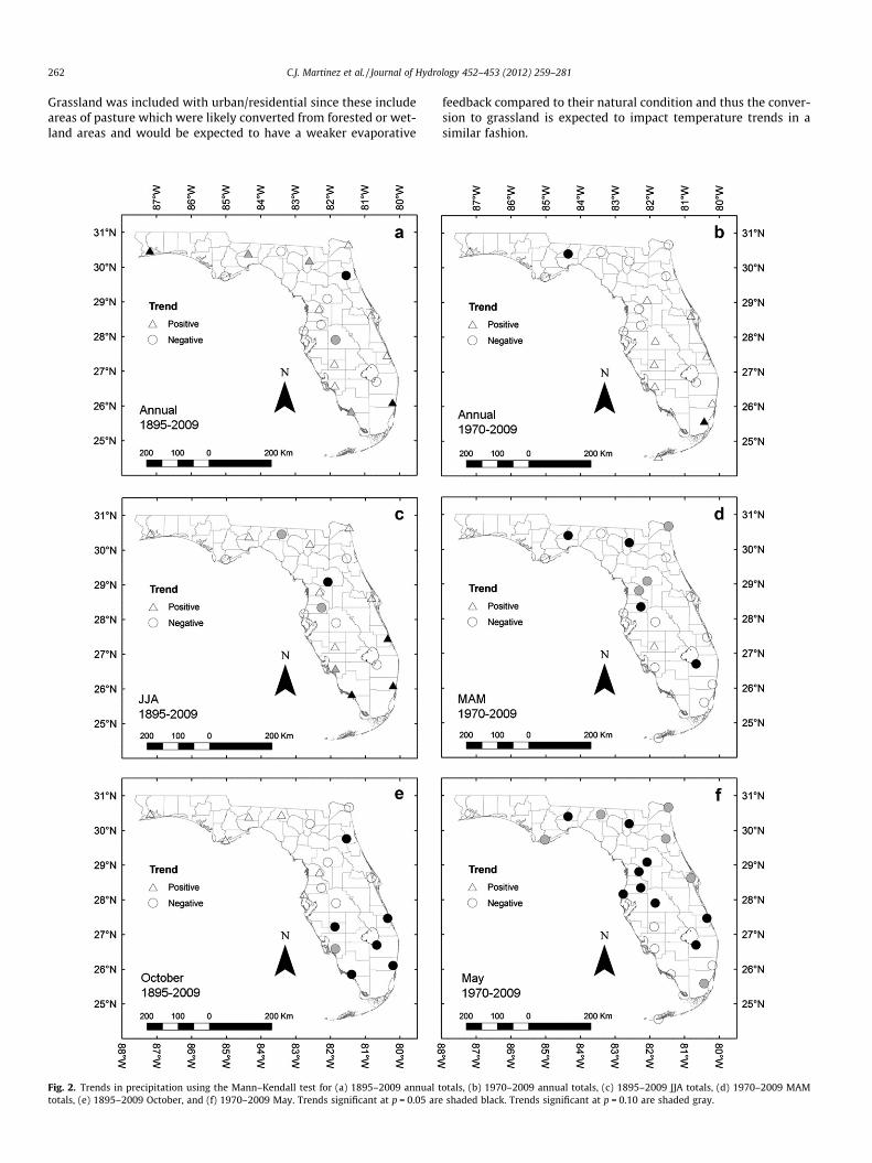
Fig. 2. Trends in precipitation using the Mann–Kendall test for (a) 1895–2009 annual ttotals, (e) 1895–2009 October, and (f) 1970–2009 May. Trends significant at p = 0.05 are

feedback compared to their natural condition and thus the conver-sion to grassland is expected to impact temperature trends in asimilar fashion.

otals, (b) 1970–2009 annual totals, (c) 1895–2009 JJA totals, (d) 1970–2009 MAMshaded black. Trends significant at p = 0.10 are shaded gray.

C.J. Martinez et al. / Journal of Hydrology 452–453 (2012) 259–281 263

3. Methods

Trends in annual, seasonal (3-month), and monthly precipita-tion, temperature (mean, maximum, and minimum), and tempera-ture range (maximum–minimum) were evaluated for both the

Fig. 3. Box-and-whisker plots of trends in precipitation using Sen’s slope for (a) 1895–20(d) 1970–2009 monthly totals. Inner box denotes the interquartile range and median, w

Table 3Number of stations with significant trends in homogenized precipitation at p < 0.05. The nuby ⁄ are field significant.

Mann–Kendall

1895–2009 1970–2009

+ � + �

Annual 2 (4) 0 (0) 1 (1) 0 (0)

Season + � + �JFM 0 (3) 0 (0) 0 (0) 1 (3)FMA 1 (1) 0 (0) 0 (1) 0 (0)MAM 0 (0) 0 (0) 0 (0) 2 (5⁄)AMJ 0 (1) 0 (0) 0 (0) 0 (0)MJJ 1 (1) 0 (1) 0 (0) 0 (0)JJA 3 (4⁄) 0 (3⁄) 1 (2) 0 (0)JAS 2 (3⁄) 1 (2⁄) 1 (2) 0 (0)ASO 0 (0) 0 (0) 4⁄ (5⁄) 0 (0)SON 0 (0) 0 (0) 1 (2) 0 (0)OND 1 (1) 0 (0) 2 (2) 0 (0)NDJ 0 (3) 0 (0) 0 (0) 2 (5)DJF 0 (1) 0 (0) 0 (0) 2 (2)

Month + � + �Jan 1 (3) 0 (0) 0 (0) 1 (1)Feb 0 (0) 1 (1) 0 (0) 3 (4)Mar 1 (2) 0 (0) 0 (0) 0 (0)Apr 0 (1) 0 (0) 2 (3) 0 (0)May 0 (0) 2 (6⁄) 0 (0) 9⁄ (13⁄

June 2 (2) 0 (1) 0 (1) 0 (0)July 1 (1) 1 (2) 1 (1) 0 (0)Aug 2 (3⁄) 1 (3⁄) 0 (0) 0 (0)Sept 0 (0) 0 (0) 1 (2) 0 (0)Oct 0 (0) 4 (7⁄) 0 (0) 0 (0)Nov 1 (2) 0 (0) 0 (0) 0 (0)Dec 0 (0) 0 (0) 0 (0) 0 (0)

period of record of the dataset (1895–2009) and recent years(1970–2009). The selection of 1970–2009 to represent the recentperiod is arbitrary and it should be noted that different resultscould potentially be found using different start and end years todefine the recent period. Analyses were performed only for stations

09 seasonal totals, (b) 1970–2009 seasonal totals, (c) 1895–2009 monthly totals, andhiskers extend to points within a distance of 1.5 times the interquartile range.

mber of stations with significant trends at p < 0.10 are in parenthesis. Values followed

Linear regression

1895–2009 1970–2009

+ � + �

3 (5⁄) 0 (0) 1 (1) 0 (0)

+ � + �1 (3) 0 (0) 0 (0) 0 (2)1 (1) 0 (0) 0 (0) 0 (0)0 (0) 0 (0) 0 (0) 2 (6⁄)0 (1) 0 (0) 0 (0) 0 (0)1 (1) 1 (1) 0 (0) 0 (0)4⁄ (4⁄) 1⁄ (3⁄) 1 (4⁄) 0 (0)3⁄ (3⁄) 1⁄ (1⁄) 2 (3) 0 (0)0 (0) 0 (0) 5⁄ (6⁄) 0 (0)0 (1) 0 (0) 1 (3) 0 (0)1 (1) 0 (1) 2 (2) 0 (0)2 (3) 0 (0) 0 (0) 2 (3)1 (1) 0 (0) 0 (0) 1 (1)

+ � + �1 (3) 0 (0) 0 (0) 0 (0)0 (1) 1 (1) 0 (0) 0 (3)0 (1) 0 (0) 0 (0) 0 (1)1 (1) 0 (0) 0 (4) 0 (0)

) 0 (0) 0 (1) 0 (0) 7⁄ (9⁄)2 (2) 0 (0) 0 (1) 0 (0)1⁄ (1⁄) 2⁄ (2⁄) 1 (2) 0 (0)2⁄ (3⁄) 2⁄ (4⁄) 1 (2) 0 (0)0 (0) 0 (0) 1 (2) 0 (0)0 (1⁄) 3 (6⁄) 0 (1) 0 (0)1 (4) 0 (0) 0 (0) 0 (1)0 (2) 0 (1) 0 (0) 0 (0)

264 C.J. Martinez et al. / Journal of Hydrology 452–453 (2012) 259–281

with complete records for the given time period. This resulted in19 and 21 stations included in the evaluation of precipitationtrends for the 1895–2009 and 1970–2009 time periods, respec-tively (Table 1). Trends were evaluated using both the non-para-metric Mann–Kendall test (Helsel and Hirsch, 2002; Kendall,1975; Mann, 1945) and least-squares linear regression. Signifi-cance of trends were evaluated at the 0.05 and 0.10 levels. Themagnitude of trends were evaluated using Sen’s slope (Sen,1968). The Mann–Kendall test and Sen’s slope were chosen dueto their resistance to outliers compared to ordinary least-squaresregression. As such, results are discussed primarily on context ofthese non-parametric techniques. Results based on linear regres-sion are thus included to be complementary and in the interestof completeness.

Spatial correlation is an often neglected aspect of evaluating thecollective significance of trends (Douglas et al., 2000). Spatial cor-relation results in a reduction of the effective degrees of freedom ofthe dataset as each station is not an independent observation(Livezey and Chen, 1983). Thus, the number of stations with locallysignificant trends is insufficient in determining the collective, orfield, significance of a dataset (Wilks, 2006). A test for field signif-icance addresses the question as to whether the number of statis-tically significant local trends is greater than would have beenfound by chance. To determine the field significance of trends aMonte Carlo permutation approach was used (Livezey and Chen,1983). In this approach station time series were reshuffled ran-domly 1000 times. Each station time series was reshuffled intothe same new order at each iteration, preserving the spatial corre-lation between the time series. After each permutation the numberof locally significant trends was noted for a given level of signifi-cance. The number of locally significant trends that must be ex-ceeded to be deemed field significant was determined from thefrequency distribution of locally significant trends from the 1000permutations. The rationale of this approach is that under the null

Table 4Number of stations with significant trends in mean temperature at p < 0.05. The number offield significant.

Mann–Kendall

1895–2009 1970–2009

+ � + �

Annual 14⁄ (14⁄) 4⁄ (5⁄) 15⁄ (17⁄) 0 (0

Season + � + �JFM 5 (7⁄) 2 (3⁄) 7 (11⁄) 0 (0FMA 7 (9) 0 (1) 4 (8⁄) 0 (0MAM 9⁄ (11⁄) 3⁄ (5⁄) 4 (6) 0 (0AMJ 13⁄ (13⁄) 2⁄ (3⁄) 12⁄ (12⁄) 0 (0MJJ 14⁄ (14⁄) 2⁄ (3⁄) 14⁄ (16⁄) 0 (0JJA 15⁄ (15⁄) 2⁄ (2⁄) 17⁄ (17⁄) 0 (0JAS 15⁄ (15⁄) 1⁄ (3⁄) 15⁄ (17⁄) 0 (0ASO 14⁄ (15⁄) 2⁄ (3⁄) 15⁄ (15⁄) 0 (0SON 13⁄ (13⁄) 1⁄ (2⁄) 7 (8⁄) 0 (0OND 12⁄ (14⁄) 1⁄ (1⁄) 1 (2) 0 (0NDJ 9⁄ (11⁄) 1⁄ (1⁄) 0 (0) 0 (0DJF 9 (11⁄) 1 (1⁄) 0 (1) 0 (0

Month + � + �Jan 0 (1) 1 (2) 0 (3) 0 (0Feb 6 (11⁄) 0 (0) 6 (13⁄) 0 (0Mar 3 (4) 2 (3) 0 (0) 0 (0Apr 9⁄ (12⁄) 0 (0) 1 (1) 0 (0May 11⁄ (13⁄) 1⁄ (1⁄) 11⁄ (13⁄) 0 (0June 13⁄ (14⁄) 2⁄ (3⁄) 11⁄ (12⁄) 0 (0July 16⁄ (16⁄) 1⁄ (2⁄) 14⁄ (15⁄) 0 (0Aug 15⁄ (15⁄) 2⁄ (2⁄) 17⁄ (18⁄) 0 (0Sept 14⁄ (14⁄) 2⁄ (3⁄) 7⁄ (7⁄) 0 (0Oct 10⁄ (10⁄) 1⁄ (1⁄) 4 (7) 0 (0Nov 12⁄ (12⁄) 0 (1⁄) 0 (0) 0 (0Dec 10⁄ (11⁄) 0 (0) 0 (0) 0 (0

hypothesis of no trend, each random permutation of the data isequally likely (Burn and Hag Elnur, 2002). Similar permutationand bootstrap tests for field significance have been used in severalprevious studies (e.g. Burn and Hag Elnur, 2002; Kunkel et al.,1999; Suppiah and Hennessy, 1998; Wilks, 1996).

In the USHCN Version 2 Serial Monthly Dataset temperaturevariables were evaluated and corrected for undocumentedchangepoints, but precipitation was not. Thus an additionalhomogenization step may be required for the evaluation of precip-itation trends. For this work homogenization of monthly precipita-tion records was conducted using the ‘‘Climatol’’ version 2.1contributed package (Guijarro, 2011) to the R statistical package(R Development Core Team, 2011). For homogenization, monthlyprecipitation was power transformed (y = x0.4) and then normal-ized as ratios to mean values. Outliers greater than five timesthe standard deviation were deleted. In the Climatol package ref-erence series for each station were computed as an average ofup to the nearest ten neighbors, weighted by an inverse distancefunction. The difference between the observed and reference ser-ies were used to identify breaks. It should be noted that breaksdue to common network history (e.g. simultaneous changes ininstruments or practices) are not easily detectable. Break detectionwas performed on the serial monthly series using the StandardNormal Homogeneity Test (SNHT) (Alexandersson, 1986) in twosteps; the first step evaluated the series using a running windowof 60 months and the second step evaluated the entire series.The procedure was repeated in the Climatol package until no addi-tional breaks were found. The critical value of the SNHT test statis-tic corresponding to 95% significance was obtained from Khaliqand Ouarda (2007). For this work, trend analyses were conductedfor both homogenized and non-homogenized precipitation datasince applying homogenization procedures has been shown to in-crease data inhomogeneities in precipitation in some cases(Venema et al., 2012).

stations with significant trends at p < 0.10 are in parenthesis. Values followed by ⁄ are

Linear regression

1895–2009 1970–2009

+ � + �

) 14⁄ (14⁄) 3⁄ (5⁄) 16⁄ (17⁄) 0 (0)

+ � + �) 5 (8⁄) 2 (4⁄) 4 (8) 0 (0)) 9 (11⁄) 0 (2⁄) 6 (10⁄) 0 (0)) 10⁄ (11⁄) 2⁄ (6⁄) 5 (8⁄) 0 (0)) 13⁄ (13⁄) 2⁄ (3⁄) 12⁄ (13⁄) 0 (0)) 14⁄ (14⁄) 2⁄ (3⁄) 14⁄ (15⁄) 0 (0)) 15⁄ (15⁄) 2⁄ (3⁄) 17⁄ (17⁄) 0 (0)) 15⁄ (15⁄) 1⁄ (3⁄) 16⁄ (16⁄) 0 (0)) 14⁄ (14⁄) 2⁄ (4⁄) 15⁄ (16⁄) 0 (0)) 13⁄ (13⁄) 2⁄ (2⁄) 7 (8⁄) 0 (0)) 14⁄ (14⁄) 1⁄ (1⁄) 1 (3) 0 (0)) 10⁄ (11⁄) 1⁄ (1⁄) 0 (0) 0 (0)) 8 (9⁄) 1 (1⁄) 1 (1) 0 (0)

+ � + �) 0 (0) 2 (4) 0 (1) 0 (0)) 6 (9) 0 (0) 10⁄ (13⁄) 0 (0)) 4 (4) 1 (4) 0 (1) 0 (0)) 9⁄ (11⁄) 0 (1⁄) 0 (1) 0 (0)) 12⁄ (13⁄) 1⁄ (2⁄) 12⁄ (12⁄) 0 (0)) 14⁄ (14⁄) 1⁄ (3⁄) 12⁄ (15⁄) 0 (0)) 16⁄ (17⁄) 1⁄ (1⁄) 14⁄ (15⁄) 0 (0)) 15⁄ (15⁄) 1⁄ (2⁄) 17⁄ (18⁄) 0 (0)) 14⁄ (14⁄) 3⁄ (4⁄) 6 (6) 0 (0)) 10⁄ (10⁄) 1⁄ (1⁄) 8 (9⁄) 0 (0)) 13⁄ (14⁄) 0 (0) 0 (0) 0 (0)) 11⁄ (12⁄) 0 (0) 0 (0) 0 (0)

C.J. Martinez et al. / Journal of Hydrology 452–453 (2012) 259–281 265

To evaluate the potential impact of station siting on historicaltrends we employ the station siting ratings from the Surface Sta-tions Project (Watts, 2009) as also used by Menne et al. (2010)and Fall et al. (2011). The Surface Stations Project was a volunteer

Fig. 4. Trends in mean temperature using the Mann–Kendall test for (a) 1895–2009 annuvalues, (e) 1895–2009 July, and (f) 1970–2009 August. Trends significant at p = 0.05 are

effort to classify USHCN station exposure conditions based on vi-sual inspection. Stations were classified using a rating systembased on the criteria used to develop the USCRN (NOAA andNESDIS, 2002). Stations are rated on a scale from 1 to 5, with 1

al values, (b) 1970–2009 annual values, (c) 1895–2009 JJA values, (d) 1970–2009 JJAshaded black. Trends significant at p = 0.10 are shaded gray.

266 C.J. Martinez et al. / Journal of Hydrology 452–453 (2012) 259–281

indicating the best station siting and 5 the poorest (Table 1 andFig. 1). Since there were few stations classified as CRN 1 or CRN5, we combined stations into two groups of CRN 1&2 (good stationsiting) and CRN 4&5 (poor station siting) stations for comparison.Stations were aggregated into their respective classes by first com-puting station anomalies relative to a 30-year baseline period of1971–2000. Anomalies were then averaged across all stations ina given USCRN group. The statistical difference between groupswere evaluated by evaluating the significance of the trend in thedifferences of the time series between groups.

To evaluate the potential impact of regional land use/land coveron temperature trends the percentage of each land use within a 10-km radius of each station was extracted from the NLCD 2006 (Table1 and Fig. 1). The radius of 10-km was chosen following the work ofGallo et al. (1996) who found significant differences in diurnaltemperature range between urban and rural stations based onthe predominant land use within this distance. Land use categorieswere extracted from the NLCD 2006 using the Geographic Informa-tion System software ArcMap (www.esri.com). It is important tonote that the station siting class previously referred to does notnecessarily correspond to the surrounding land use/land cover.Rather, the station siting classification reflects the conditions in

Fig. 5. Count of significant trends (p = 0.05) in mean temperature at each station for (a)2009 months. Top value is the number of significantly positive trends. Bottom value is t

the immediate vicinity of a given station while the surroundingland use/land cover reflects more regional impacts.

4. Results and discussion

4.1. Trends in non-homogenized precipitation

Few field significant trends in non-homogenized precipitationwere found for either the 1895–2009 or 1970–2009 time periods(Table 2). Trends in 1895–2009 annual total precipitation werefound to be significant at seven stations (five positive and two neg-ative) at p < 0.10 using both the Mann–Kendall test or linear regres-sion (field significant results were also found at p < 0.05 at fivestations using linear regression), but were not field significant forthe recent period (1970–2009) (Fig. 2 and Table 2). The lack of signif-icance in the recent period is consistent with the results of Lette-nmaier et al. (1994) for the period 1948–1988. The mean ofstation trends in annual rainfall using Sen’s slope was found to be0.285 and -0.177 mm year�1 for the 1895–2009 and 1970–2009periods, respectively.

Field significant trends in non-homogenized precipitation atp < 0.05 were only found during the June–August (JJA) season

1895–2009 seasons, (b) 1970–2009 seasons, (c) 1895–2009 months, and (d) 1970–he number of significantly negative trends.

C.J. Martinez et al. / Journal of Hydrology 452–453 (2012) 259–281 267

for the 1895–2009 period (Fig. 2 and Table 2), with locally signif-icant positive trends occurring in the southern portion of thestate. Field significant trends at p < 0.10 were also found for the

Fig. 6. Box-and-whisker plots of trends in mean temperature using Sen’s slope for (a) 1values, and (d) 1970–2009 monthly values. Inner box denotes the interquartile range anrange.

Table 5Number of stations with significant trends in maximum temperature at p < 0.05. The numbeare field significant.

Mann–Kendall

1895–2009 1970–2009

+ � + �

Annual 13⁄ (13⁄) 3⁄ (3⁄) 11⁄ (12⁄) 2⁄ (2⁄

Season + � + �JFM 9⁄ (11⁄) 3⁄ (3⁄) 8⁄ (12⁄) 0 (0)FMA 10⁄ (10⁄) 1⁄ (2⁄) 9⁄ (10⁄) 0 (0)MAM 11⁄ (11⁄) 2⁄ (3⁄) 5 (8⁄) 0 (0)AMJ 11⁄ (12⁄) 3⁄ (4⁄) 8⁄ (9⁄) 1⁄ (1⁄

MJJ 11⁄ (11⁄) 3⁄ (4⁄) 10⁄ (11⁄) 1⁄ (1⁄

JJA 12⁄ (13⁄) 2⁄ (5⁄) 8⁄ (9⁄) 1⁄ (1⁄

JAS 13⁄ (13⁄) 4⁄ (5⁄) 8⁄ (9⁄) 2⁄ (2⁄

ASO 12⁄ (13⁄) 4⁄ (5⁄) 8⁄ (9⁄) 3⁄ (3⁄

SON 13⁄ (14⁄) 2⁄ (2⁄) 6⁄ (7⁄) 2⁄ (2⁄

OND 13⁄ (15⁄) 1⁄ (2⁄) 4 (5) 0 (1)NDJ 12⁄ (12⁄) 1⁄ (2⁄) 1 (1) 0 (0)DJF 11⁄ (11⁄) 1⁄ (1⁄) 2 (6) 0 (0)

Month + � + �Jan 6 (8) 1 (1) 4 (6) 0 (0)Feb 11⁄ (11⁄) 0 (0) 6 (10⁄) 0 (0)Mar 7⁄ (7⁄) 2⁄ (2⁄) 2 (4) 0 (0)Apr 11⁄ (11⁄) 1⁄ (1⁄) 0 (2) 0 (2)May 11⁄ (12⁄) 2⁄ (3⁄) 11⁄ (13⁄) 0 (0)June 11⁄ (11⁄) 3⁄ (6⁄) 5 (6) 0 (0)July 14⁄ (14⁄) 1⁄ (1⁄) 8⁄ (8⁄) 1⁄ (1⁄

Aug 12⁄ (12⁄) 4⁄ (5⁄) 9⁄ (9⁄) 0⁄ (1⁄

Sept 12⁄ (12⁄) 4⁄ (5⁄) 5⁄ (5⁄) 2⁄ (4⁄

Oct 13⁄ (13⁄) 1⁄ (1⁄) 5 (5) 0 (0)Nov 12⁄ (13⁄) 1⁄ (1⁄) 2 (3) 0 (0)Dec 12⁄ (12⁄) 1⁄ (1⁄) 0 (0) 0 (0)

July–September (JAS) season for the 1895–2009 period. Field sig-nificant trends at p < 0.10 were only found during the March–May(MAM) season for the 1970–2009 period with locally significant

895–2009 seasonal values, (b) 1970–2009 seasonal values, (c) 1895–2009 monthlyd median, whiskers extend to points within a distance of 1.5 times the interquartile

r of stations with significant trends at p < 0.10 are in parenthesis. Values followed by ⁄

Linear regression

1895–2009 1970–2009

+ � + �

) 13⁄ (14⁄) 3⁄ (3⁄) 17⁄ (17⁄) 5⁄ (5⁄)

+ � + �10⁄ (11⁄) 3⁄ (3⁄) 9⁄ (9⁄) 0 (0)10⁄ (11⁄) 1⁄ (1⁄) 9⁄ (9⁄) 0 (0)11⁄ (11⁄) 3⁄ (3⁄) 8⁄ (9⁄) 0 (0)

) 11⁄ (12⁄) 3⁄ (5⁄) 7⁄ (10⁄) 1⁄ (1⁄)) 11⁄ (12⁄) 3⁄ (3⁄) 9⁄ (11⁄) 1⁄ (1⁄)) 13⁄ (13⁄) 2⁄ (4⁄) 8⁄ (8⁄) 1⁄ (1⁄)) 13⁄ (13⁄) 5⁄ (5⁄) 8⁄ (8⁄) 2⁄ (3⁄)) 12⁄ (12⁄) 5⁄ (5⁄) 7⁄ (8⁄) 3⁄ (3⁄)) 13⁄ (14⁄) 2⁄ (2⁄) 5⁄ (7⁄) 2⁄ (2⁄)

13⁄ (16⁄) 1⁄ (2⁄) 4 (5) 0 (2)12⁄ (12⁄) 1⁄ (2⁄) 1 (2) 0 (0)11⁄ (11⁄) 1⁄ (2⁄) 4 (7) 0 (0)

+ � + �6 (7) 1 (3) 1 (3) 0 (0)11⁄ (11⁄) 0 (0) 7 (11⁄) 0 (0)7⁄ (7⁄) 2⁄ (2⁄) 3 (5) 0 (0)11⁄ (11⁄) 1⁄ (1⁄) 2 (2) 1 (1)10⁄ (11⁄) 2⁄ (3⁄) 11⁄ (12⁄) 0 (0)10⁄ (11⁄) 3⁄ (5⁄) 5 (8) 0 (0)

) 13⁄ (14⁄) 1⁄ (1⁄) 8⁄ (8⁄) 1⁄ (1⁄)) 12⁄ (13⁄) 4⁄ (5⁄) 9 (10⁄) 0 (1⁄)) 12⁄ (12⁄) 4⁄ (5⁄) 5⁄ (5⁄) 4⁄ (5⁄)

12⁄ (13⁄) 1⁄ (2⁄) 5 (5) 0 (0)13⁄ (14⁄) 1⁄ (1⁄) 2 (3) 0 (0)12⁄ (12⁄) 1⁄ (1⁄) 0 (1) 0 (0)

268 C.J. Martinez et al. / Journal of Hydrology 452–453 (2012) 259–281

negative trends in the central and northern parts of the state. Sixstations were also found to be field significant at p < 0.10 in theAugust–October (ASO) season using linear regression, but were

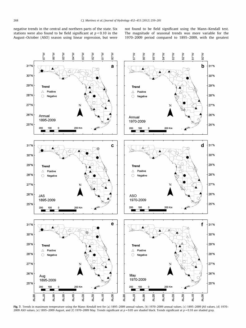
Fig. 7. Trends in maximum temperature using the Mann–Kendall test for (a) 1895–20092009 ASO values, (e) 1895–2009 August, and (f) 1970–2009 May. Trends significant at p

not found to be field significant using the Mann–Kendall test.The magnitude of seasonal trends was more variable for the1970–2009 period compared to 1895–2009, with the greatest

annual values, (b) 1970–2009 annual values, (c) 1895–2009 JAS values, (d) 1970–= 0.05 are shaded black. Trends significant at p = 0.10 are shaded gray.

C.J. Martinez et al. / Journal of Hydrology 452–453 (2012) 259–281 269

variability between stations occurring in the summer months(Fig. 3). Mean trends in seasonal precipitation were 0.053 and�0.126 mm year�1 for the 1895–2009 and 1970–2009 periods,respectively.

For monthly results, field significant, and generally negative,trends at p < 0.05 were only found for the month of Octoberand May for the 1895–2009 and 1970–2009 periods, respectively(Fig. 2 and Table 2). Field significant results at p < 0.10 were alsofound for the month of May for 1895–2009 using the Mann–Ken-dall test only and for August for 1895–2009 using linear regres-sion only. The significant reduction in May precipitation in the1970–2009 period indicates a delayed onset of the wet season(typically from June to September) in much of the state. Thiswork did not find the significant increases in the months of Jan-uary, February, and November found by Lettenmaier et al. (1994)for the period 1948–1988, however the significant decreasingtrends in October are consistent between the two studies. As withthe seasonal trends, monthly trends were more variable betweenstations for the 1970–2009 period compared to 1895–2009(Fig. 3) with mean trends in monthly precipitation of 0.004 and�0.056 mm year�1 for the 1895–2009 and 1970–2009 periods,respectively.

Fig. 8. Count of significant trends (p = 0.05) in maximum temperature at each station f1970–2009 months. Top value is the number of significantly positive trends. Bottom va

4.2. Trends in homogenized precipitation

Homogenization of the monthly rainfall series identified 22artificial breaks in the data at 11 stations (Table 1). However, thenumber of significant trends in annual, seasonal, and monthlyprecipitation (Table 3) was generally similar to that found fornon-homogenized precipitation (Table 2). Unlike the trends innon-homogenized precipitation, no significant negative trendswere found in annual precipitation, and there was a notable reduc-tion of significant negative trends in seasonal precipitation but notin monthly precipitation. Notable differences between the homog-enized and non-homogenized trend results include field significant(at p < 0.05) positive trends in the ASO season during the 1970–2009 period, field significant (at p < 0.10) trends (both positiveand negative) in August precipitation in the 1895–2009 period,and a lessening in the level of field significance (to p < 0.10) inOctober precipitation during the 1895–2009 period.

4.3. Trends in Mean Temperature

Field significant trends in annual mean temperature were foundfor both the 1895–2009 and 1970–2009 time periods (Table 4). For

or (a) 1895–2009 seasons, (b) 1970–2009 seasons, (c) 1895–2009 months, and (d)lue is the number of significantly negative trends.

Fig. 9. Box-and-whisker plots of trends in maximum temperature using Sen’s slope for (a) 1895–2009 seasonal values, (b) 1970–2009 seasonal values, (c) 1895–2009monthly values, and (d) 1970–2009 monthly values. Inner box denotes the interquartile range and median, whiskers extend to points within a distance of 1.5 times theinterquartile range.

Table 6Number of stations with significant trends in minimum temperature at p < 0.05. The number of stations with significant trends at p < 0.10 are in parenthesis. Values followed by ⁄are field significant.

Mann–Kendall Linear Regression

1895–2009 1970–2009 1895–2009 1970–2009

+ � + � + � + �

Annual 10⁄ (10⁄) 5⁄ (6⁄) 13⁄ (13⁄) 0 (0) 10⁄ (11⁄) 5⁄ (5⁄) 13⁄ (14⁄) 0 (0)

Season + � + � + � + �JFM 3 (4⁄) 4 (6⁄) 3 (7) 0 (0) 3 (4) 5 (6) 4 (7) 0 (0)FMA 6⁄ (7⁄) 3⁄ (5⁄) 7 (8) 0 (0) 6⁄ (7⁄) 4⁄ (4⁄) 7 (8) 0 (0)MAM 7⁄ (9⁄) 6⁄ (7⁄) 3 (5) 0 (1) 9⁄ (9⁄) 5⁄ (7⁄) 6 (7) 0 (0)AMJ 11⁄ (11⁄) 3⁄ (3⁄) 7⁄ (9⁄) 0 (0) 11⁄ (11⁄) 2⁄ (3⁄) 7 (8⁄) 0 (0)MJJ 14⁄ (14⁄) 1⁄ (1⁄) 15⁄ (17⁄) 0 (0) 13⁄ (14⁄) 1⁄ (2⁄) 16⁄ (16⁄) 0 (0)JJA 15⁄ (16⁄) 1⁄ (2⁄) 15⁄ (17⁄) 0 (0) 15⁄ (15⁄) 1⁄ (2⁄) 16⁄ (20⁄) 0 (0)JAS 13⁄ (13⁄) 2⁄ (2⁄) 16⁄ (16⁄) 0 (0) 13⁄ (13⁄) 2⁄ (2⁄) 18⁄ (19⁄) 0 (0)ASO 10⁄ (11⁄) 3⁄ (4⁄) 14⁄ (14⁄) 0 (0) 11⁄ (11⁄) 3⁄ (4⁄) 14⁄ (15⁄) 0 (0)SON 9⁄ (10⁄) 3⁄ (3⁄) 9⁄ (11⁄) 0 (0) 10⁄ (10⁄) 1⁄ (3⁄) 7⁄ (11⁄) 0 (0)OND 7⁄ (8⁄) 2⁄ (2⁄) 4 (6) 0 (0) 8⁄ (8⁄) 1⁄ (2⁄) 6 (6) 0 (0)NDJ 4 (5) 0 (2) 0 (0) 0 (0) 4 (5) 2 (3) 0 (0) 0 (0)DJF 5 (5) 1 (2) 2 (3) 0 (0) 4 (5) 2 (4) 1 (5) 0 (0)

Month + � + � + � + �Jan 0 (0) 5 (6) 0 (1) 0 (0) 0 (0) 5 (6) 0 (0) 0 (0)Feb 4 (4) 0 (0) 6 (10) 0 (0) 4 (5) 0 (0) 7 (10⁄) 0 (0)Mar 1 (5⁄) 3 (4⁄) 1 (3) 0 (0) 1 (6⁄) 4 (4⁄) 3 (3) 0 (0)Apr 5⁄ (6⁄) 2⁄ (3⁄) 2 (2) 0 (1) 4 (6⁄) 2 (4⁄) 2 (3) 0 (0)May 9⁄ (11⁄) 1⁄ (1⁄) 6 (10⁄) 0 (0) 8⁄ (10⁄) 1⁄ (1⁄) 6 (9⁄) 0 (0)June 15⁄ (15⁄) 1⁄ (1⁄) 14⁄ (15⁄) 0 (0) 15⁄ (15⁄) 1⁄ (1⁄) 14⁄ (15⁄) 0 (0)July 15⁄ (15⁄) 2⁄ (2⁄) 16⁄ (18⁄) 0 (0) 15⁄ (17⁄) 2⁄ (2⁄) 18⁄ (18⁄) 0 (0)Aug 13⁄ (13⁄) 2⁄ (2⁄) 14⁄ (16⁄) 0 (0) 13⁄ (14⁄) 2⁄ (2⁄) 17⁄ (18⁄) 0 (0)Sept 11⁄ (11⁄) 2⁄ (4⁄) 8⁄ (10⁄) 0 (0) 11⁄ (11⁄) 2⁄ (4⁄) 9⁄ (10⁄) 0 (0)Oct 4 (4) 2 (4) 6 (11⁄) 0 (0) 4 (6⁄) 2 (5⁄) 10⁄ (10⁄) 0 (0)Nov 5 (6) 0 (0) 0 (0) 0 (0) 5 (5) 0 (0) 0 (0) 0 (0)Dec 6 (6) 0 (0) 0 (0) 0 (0) 6 (6) 0 (0) 0 (1) 0 (0)

270 C.J. Martinez et al. / Journal of Hydrology 452–453 (2012) 259–281

the 1895–2009 period, positive trends were found throughout thestate while significant negative trends were mainly confined to the

more northerly part of the state (Fig. 4). This result is consistentwith that of Lettenmaier et al. (1994) for the period 1948–1988.

C.J. Martinez et al. / Journal of Hydrology 452–453 (2012) 259–281 271

No locally significant negative trends were found for the 1970–2009 period. The mean of station trends for annual mean temper-ature was found to be 0.005 and 0.017 �C year�1 for the 1895–2009and 1970–2009 periods using Sen’s slope, respectively.

Fig. 10. Trends in minimum temperature using the Mann–Kendall test for (a) 1895–2002009 JAS values, (e) 1895–2009 July, and (f) 1970–2009 July. Trends significant at p = 0.

Generally positive field-significant trends in seasonal mean tem-perature were found between the MAM and November–January(NDJ) seasons for the 1895–2009 period, with the largest numberof locally significant trends found during the middle of the year

9 annual values, (b) 1970–2009 annual values, (c) 1895–2009 JJA values, (d) 1970–05 are shaded black. Trends significant at p = 0.10 are shaded gray.

272 C.J. Martinez et al. / Journal of Hydrology 452–453 (2012) 259–281

(Table 4 and Fig. 4). Field significant, positive trends were confinedto the April–June (AMJ) to ASO seasons for the 1970–2009 period.No significant negative trends were found for the 1970–2009 timeperiod. This increase in summer mean temperature may be par-tially explained for southern Florida to the large-scale conversionfrom marsh to agricultural lands that occurred during the 20thcentury (Pielke et al., 1999). Fig. 5a and b shows the spatialdistribution of locally significant positive and negative trends inseasonal mean temperature for both time periods. The highest con-centration of significant positive trends for the 1895–2009 periodwere found along the southeast coast and in the west-central por-tion of the state (Fig. 5), while spatial coherence was less for the1970–2009 period. The north–south gradient is consistent withthat found by Lu et al. (2005) for seasonal temperature. Seasonaltrends were greater, overall, for the 1970–2009 period (mean of0.016 �C year�1) compared to 1895–2009 (mean of 0.005 �C year�1)with the largest magnitudes occurring during the winter and springseasons (Fig. 6).

Field significant trends in monthly mean temperature werefound between April to December and May to September for the1895–2009 and 1970–2009 periods, respectively (Table 4). Unlikethe work of Lettenmaier et al. (1994), this work did not detect sig-

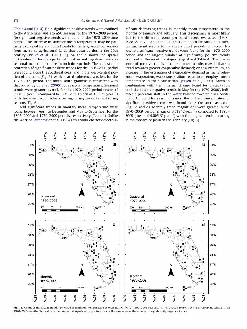
Fig. 11. Count of significant trends (p = 0.05) in minimum temperature at each station1970–2009 months. Top value is the number of significantly positive trends. Bottom va

nificant decreasing trends in monthly mean temperature in themonths of January and February. This discrepancy is most likelydue to the different recent period of record evaluated (1948–1988 vs. 1970–2009) and illustrates the need for caution in inter-preting trend results for relatively short periods of record. Nolocally significant negative trends were found for the 1970–2009period and the largest number of significantly positive trendsoccurred in the month of August (Fig. 4 and Table 4). The preva-lence of positive trends in the summer months may indicate atrend towards greater evaporative demand; or at a minimum, anincrease in the estimation of evaporative demand as many refer-ence evaporation/evapotranspiration equations employ meantemperature in their calculation (Jensen et al., 1990). Taken incombination with the minimal change found for precipitation(and the notable negative trends in May for the 1970–2009), indi-cates a potential shift in the water balance towards drier condi-tions. As found for seasonal trends, the highest concentration ofsignificant positive trends was found along the southeast coast(Fig. 5c and d). Monthly trend magnitudes were greater in the1970–2009 period (mean of 0.018 �C year�1) compared to 1895–2009 (mean of 0.005 �C year�1) with the largest trends occurringin the months of January and February (Fig. 6).

for (a) 1895–2009 seasons, (b) 1970–2009 seasons, (c) 1895–2009 months, and (d)lue is the number of significantly negative trends.

Fig. 12. Box-and-whisker plots of trends in minimum temperature using Sen’s slope for (a) 1895–2009 seasonal values, (b) 1970–2009 seasonal values, (c) 1895–2009monthly values, and (d) 1970–2009 monthly values. Inner box denotes the interquartile range and median, whiskers extend to points within a distance of 1.5 times theinterquartile range.

C.J. Martinez et al. / Journal of Hydrology 452–453 (2012) 259–281 273

4.4. Trends in maximum temperature

Field significant trends in annual maximum temperature werefound for both the 1895–2009 (mean of 0.007 �C year�1) and1970–2009 (mean of 0.014 �C year�1) time periods (Table 5 andFig. 7). Locally significant positive trends were mainly found inthe west-central, southern peninsula, and panhandle portions ofthe state (Fig. 7a and b) and generally coincide with the results pre-sented by Menne et al. (2009).

Seasonal maximum temperature trends were field significantfor all seasons in the 1895–2009 period and all seasons except be-tween the seasons of October–December (OND) and December–February (DJF) in the 1970–2009 time period (Table 5), with thelargest number of locally significant trends occurring in the JASand ASO seasons for the 1895–2009 and 1970–2009 time periods,respectively (Fig. 7). Locally significant trends were found for allseasons at stations along the southeastern coast for the 1895–2009 period (Fig. 8a); while no clear clustering was evident forthe 1970–2009 period (Figs. 8b). However, the increasing trendsfound in the southeast portion of the state were consistent withthe results found by Marshall et al. (2004b) who attributed in-creased July–August temperature to large-scale drainage of wet-lands. The variability of trends was greater for the 1970–2009period compared to 1895–2009, and the median of trends was gen-erally greater in 1970–2009 (Fig. 9a and b). The mean of stationtrends in seasonal maximum temperature was found to be 0.007and 0.013 �C year�1 for the 1895–2009 and 1970–2009 periods,respectively.

Monthly maximum temperature trends were field significantfor all months except January in the 1895–2009 period and forthe months of May, July, August, and September in the 1970–2009 time period (Table 5), with the largest number of locally sig-nificant trends occurring in August/September and May for the1895–2009 and 1970–2009 time periods, respectively (Fig. 7 andTable 5). The highest concentration of significant positive trends

were found along the southeast coast for the 1895–2009 period,while a less coherent pattern was seen for 1970–2009 (Fig. 8cand d). The variability of trends was greater for the 1970–2009 per-iod compared to 1895–2009, where the median of trends werenotably greater in 1970–2009 for the months of January, February,and May (Fig. 9c and d). The mean of station trends in monthlymaximum temperature was found to be 0.007 and 0.015 �C year�1

for the 1895–2009 and 1970–2009 periods, respectively.

4.5. Trends in minimum temperature

Field significant trends in annual minimum temperature werefound for both the 1895–2009 (mean of 0.003 �C year�1) and1970–2009 (mean of 0.020 �C year�1) time periods (Table 6 andFig. 10). No stations were found with locally significant decreasingtrends in annual minimum temperature in the 1970–2009 period.Fewer locally significant, positive trends were found in northernportions of the state (Fig. 10a and b). The clustering of significantpositive trends in the west-central and southern portions of thepeninsula in the 1895–2009 period confirm the results found byMenne et al. (2009).

Seasonal minimum temperature trends were field significantfor all seasons in the 1895–2009 period except January–March(JFM), NDJ, and DJF and all seasons between AMJ and Septem-ber–November (SON) in the 1970–2009 time period (Table 6).The largest number of locally significant trends was found in theJJA and JAS seasons for the 1895–2009 and 1970–2009 time peri-ods, respectively (Fig. 10 and Table 6). Only one station was foundwith a locally significant negative trend (p < 0.10) in seasonal min-imum temperature in the 1970–2009 period (in the MAM season).The highest concentration of significant positive trends for the1895–2009 period were found along the southeast coast and inthe west-central portion of the state (Fig. 11), while spatial coher-ence was less for the 1970–2009 period. The variability of trendswas greater for the 1970–2009 period compared to 1895–2009,

274 C.J. Martinez et al. / Journal of Hydrology 452–453 (2012) 259–281

where the median of trends was greater in 1970–2009 for all sea-sons (Fig. 12a and b). The mean of station trends in seasonal min-imum temperature was found to be 0.003 and 0.019 �C year�1 forthe 1895–2009 and 1970–2009 periods, respectively.

Monthly minimum temperature trends were field significantbetween the months of April to September and June to Septemberfor the 1895–2009 and 1970–2009 time periods, respectively(Table 6), with the largest number of locally significant trendsoccurring in the month of July (Fig. 10). As with seasonal trends,the pattern of the number of months with locally significant trendswas less spatially coherent during the 1970–2009 period comparedto 1895–2009 (Fig. 10). The variability of trends was greater for the1970–2009 period compared to 1895–2009, with greater mediantrends in the 1970–2009 for all months except March and April(Fig. 12). The mean of station trends in monthly maximum temper-ature was found to be 0.003 and 0.021 �C year�1 for the 1895–2009and 1970–2009 periods, respectively.

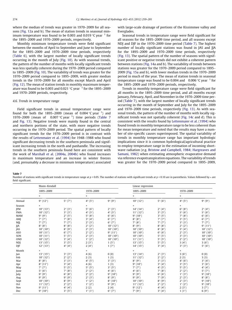
4.6. Trends in temperature range

Field significant trends in annual temperature range werefound for both the 1895–2009 (mean of 0.004 �C year�1) and1970–2009 (mean of �0.007 �C year�1) time periods (Table 7and Fig. 13). Negative trends were mainly found in the centraland northern portions of the state, with more negative trendsoccurring in the 1970–2009 period. The spatial pattern of locallysignificant trends for the 1970–2009 period is in contrast withthe results of Lettenmaier et al. (1994) for 1948–1988 who foundsignificant decreasing trends in the southern peninsula and signif-icant increasing trends in the north and panhandle. The increasingtrends in the southern peninsula found here are consistent withthe work of Marshall et al. (2004a, 2004b) who found increasesin maximum temperature and an increase in winter freezes(and, presumably a decrease in minimum temperature) associated

Table 7Number of stations with significant trends in temperature range at p < 0.05. The number offield significant.

Mann–Kendall

1895–2009 1970–2009

+ � + �

Annual 9⁄ (12⁄) 5⁄ (7⁄) 4⁄ (5⁄) 9⁄ (9⁄)

Season + � + �JFM 10⁄ (13⁄) 2⁄ (3⁄) 5⁄ (6⁄) 2⁄ (3⁄)FMA 10⁄ (12⁄) 3⁄ (3⁄) 4⁄ (5⁄) 4⁄ (5⁄)MAM 9⁄ (9⁄) 2⁄ (5⁄) 5⁄ (8⁄) 6⁄ (6⁄)AMJ 7⁄ (7⁄) 7⁄ (8⁄) 3⁄ (4⁄) 6⁄ (7⁄)MJJ 7⁄ (7⁄) 7⁄ (7⁄) 2⁄ (3⁄) 6⁄ (7⁄)JJA 8⁄ (8⁄) 8⁄ (8⁄) 2⁄ (2⁄) 10⁄ (12⁄

JAS 10⁄ (10⁄) 8⁄ (9⁄) 2⁄ (3⁄) 10⁄ (10⁄

ASO 10⁄ (11⁄) 6⁄ (7⁄) 2⁄ (2⁄) 9⁄ (11⁄)SON 10⁄ (11⁄) 5⁄ (5⁄) 2⁄ (3⁄) 10⁄ (10⁄

OND 10⁄ (12⁄) 3⁄ (4⁄) 1⁄ (2⁄) 10⁄ (10⁄

NDJ 13⁄ (15⁄) 3⁄ (5⁄) 2 (3⁄) 1 (5⁄)DJF 12⁄ (13⁄) 4⁄ (4⁄) 2 (4⁄) 1 (7⁄)

Month + � + �Jan 13⁄ (15⁄) 3⁄ (3⁄) 4 (6) 0 (0)Feb 10⁄ (12⁄) 2⁄ (2⁄) 2 (3) 1 (3)Mar 8⁄ (8⁄) 3⁄ (3⁄) 4⁄ (5⁄) 3⁄ (3⁄)Apr 8⁄ (11⁄) 3⁄ (4⁄) 4 (6) 1 (3)May 7⁄ (7⁄) 5⁄ (5⁄) 5⁄ (5⁄) 3⁄ (5⁄)June 5⁄ (6⁄) 7⁄ (8⁄) 2⁄ (2⁄) 4⁄ (6⁄)July 9⁄ (9⁄) 6⁄ (8⁄) 2⁄ (2⁄) 9⁄ (10⁄)Aug 9⁄ (9⁄) 9⁄ (9⁄) 2⁄ (3⁄) 8⁄ (9⁄)Sept 10⁄ (10⁄) 8⁄ (9⁄) 1⁄ (2⁄) 8⁄ (10⁄)Oct 11⁄ (12⁄) 2⁄ (2⁄) 1⁄ (2⁄) 9⁄ (9⁄)Nov 9⁄ (11⁄) 4⁄ (4⁄) 2 (2) 2 (4)Dec 9⁄ (10⁄) 3⁄ (5⁄) 1⁄ (1⁄) 6⁄ (7⁄)

with large-scale drainage of portions of the Kissimmee valley andEverglades.

Seasonal trends in temperature range were field significant forall seasons for the 1895–2009 time period, and all seasons exceptNDJ and DJF in the 1970–2009 time period (Table 7). The highestnumber of locally significant stations was found in JAS and JJAfor the 1895–2009 and 1970–2009 time periods, respectively(Fig. 13). The spatial pattern of the number of seasons with signif-icant positive or negative trends did not exhibit a coherent patternbetween stations (Fig. 14a and b). The variability of trends betweenstations was greater for the 1970–2009 period compared to 1895–2009 (Fig. 15a and b), with lower median trends in the 1970–2009period in much of the year. The mean of station trends in seasonaltemperature range was found to be 0.004 and �0.006 �C year�1 forthe 1895–2009 and 1970–2009 periods, respectively.

Trends in monthly temperature range were field significant forall months in the 1895–2009 time period, and all months exceptJanuary, February, April, and November in the 1970–2009 time per-iod (Table 7), with the largest number of locally significant trendsoccurring in the month of September and July for the 1895–2009and 1970–2009 time periods, respectively (Fig. 13). As with sea-sonal trends, the pattern of the number of months with locally sig-nificant trends was not spatially coherent (Fig. 14c and d). This isconsistent with the results found by Lettenmaier et al. (1994) whofound trends in monthly temperature range to be less coherent thanfor mean temperature and noted that the results may have a num-ber of site-specific causes superimposed. The spatial variability oftrends in monthly temperature range has important hydrologicimplications since it is common hydrological/agricultural practiceto employ temperature range in the estimation of incoming short-wave radiation (e.g. Bristow and Campbell, 1984; Hargreaves andSamani, 1982) when estimating atmospheric evaporative demandvia reference evapotranspiration equations. The variability of trendswas greater for the 1970–2009 period compared to 1895–2009,

stations with significant trends at p < 0.10 are in parenthesis. Values followed by ⁄ are

Linear regression

1895–2009 1970–2009

+ � + �

10⁄ (12⁄) 5⁄ (6⁄) 4⁄ (5⁄) 9⁄ (9⁄)

+ � + �14⁄ (14⁄) 2⁄ (4⁄) 6⁄ (8⁄) 2⁄ (4⁄)11⁄ (12⁄) 3⁄ (3⁄) 5⁄ (6⁄) 5⁄ (6⁄)9⁄ (10⁄) 3⁄ (5⁄) 7⁄ (8⁄) 6⁄ (6⁄)8⁄ (8⁄) 7⁄ (7⁄) 3⁄ (5⁄) 6⁄ (7⁄)7⁄ (8⁄) 7⁄ (7⁄) 3⁄ (3⁄) 7⁄ (7⁄)

) 8⁄ (9⁄) 8⁄ (8⁄) 2⁄ (2⁄) 9⁄ (11⁄)) 10⁄ (10⁄) 8⁄ (8⁄) 3⁄ (4⁄) 10⁄ (12⁄)

10⁄ (10⁄) 6⁄ (6⁄) 2⁄ (3⁄) 10⁄ (10⁄)) 10⁄ (10⁄) 5⁄ (5⁄) 3⁄ (3⁄) 10⁄ (10⁄)) 11⁄ (11⁄) 5⁄ (5⁄) 2⁄ (2⁄) 10⁄ (10⁄)

13⁄ (15⁄) 5⁄ (5⁄) 3 (4⁄) 3 (6⁄)14⁄ (15⁄) 3⁄ (4⁄) 3⁄ (3⁄) 5⁄ (6⁄)

+ � + �13⁄ (14⁄) 2⁄ (3⁄) 3 (6⁄) 0 (0)11⁄ (12⁄) 2⁄ (2⁄) 2 (3) 3 (3)8⁄ (9⁄) 3⁄ (3⁄) 4⁄ (6⁄) 3⁄ (4⁄)9⁄ (10⁄) 3⁄ (4⁄) 3⁄ (5⁄) 3⁄ (6⁄)7⁄ (7⁄) 4⁄ (5⁄) 5⁄ (5⁄) 4⁄ (4⁄)4⁄ (6⁄) 7⁄ (8⁄) 2⁄ (2⁄) 5⁄ (7⁄)9⁄ (9⁄) 6⁄ (6⁄) 1⁄ (3⁄) 9⁄ (10⁄)9⁄ (9⁄) 7⁄ (9⁄) 2⁄ (3⁄) 8⁄ (8⁄)10⁄ (10⁄) 8⁄ (9⁄) 2⁄ (3⁄) 9⁄ (10⁄)11⁄ (12⁄) 2⁄ (2⁄) 1⁄ (2⁄) 9⁄ (10⁄)9⁄ (12⁄) 4⁄ (4⁄) 2 (3⁄) 3 (7⁄)7⁄ (9⁄) 3⁄ (4⁄) 1 (1⁄) 6 (9⁄)

Fig. 13. Trends in temperature range using the Mann–Kendall test for (a) 1895–2009 annual values, (b) 1970–2009 annual values, (c) 1895–2009 JAS values, (d) 1970–2009JJA values, (e) 1895–2009 September, and (f) 1970–2009 July. Trends significant at p = 0.05 are shaded black. Trends significant at p = 0.10 are shaded gray.

C.J. Martinez et al. / Journal of Hydrology 452–453 (2012) 259–281 275

with lower median trends in the 1970–2009 for most months(Fig. 15c and 15d). The mean of station trends in monthly minimumtemperature was found to be 0.004 and �0.006 �C year�1 for the1895–2009 and 1970–2009 periods, respectively.

4.7. Evaluation of temperature trends based on station siting

Fig. 16 shows the Mann–Kendall trend results for the 1895–2009 and 1970–2009 periods for the stations rated as CRN 1&2

Fig. 14. Count of significant trends (p = 0.05) in temperature range at each station for (a) 1895–2009 seasons, (b) 1970–2009 seasons, (c) 1895–2009 months, and (d) 1970–2009 months. Top value is the number of significantly positive trends. Bottom value is the number of significantly negative trends.

276 C.J. Martinez et al. / Journal of Hydrology 452–453 (2012) 259–281

and CRN 4&5. Also shown are the results for the two stations ratedas CRN 5. Due to the limited number of CRN 5 stations, drawingdefinitive results by comparison to stations with good siting(CRN 1&2) should be made with caution. Significant differences be-tween CRN 1&2 stations and CRN 4&5 stations were found formean temperature, minimum temperature, and temperature rangebut not for maximum temperature in the 1895–2009 period. Thissignificant difference in mean and minimum temperatures is incontrast with the results found by Fall et al. (2011), who only foundsignificant differences between station classes for temperaturerange in the 1895–2009 period in their evaluation of stationsacross the conterminous United States. For the 1970–2009 period,significant differences between CRN 1&2 stations and CRN 4&5 sta-tions were found for mean temperature, maximum temperature,and temperature range but were not found for minimum temper-ature. As found by Fall et al. (2011), maximum temperature trendsat CRN 1&2 stations were found to be greater than that found formore poorly sited stations (CRN 4&5). In contrast with the resultsfound by Fall et al. (2011), no significant differences were found inminimum temperature in the recent period (1970–2009). At poorlysited stations associated with urbanization effects such as shading,aerosols, irrigated vegetation, and differences in thermal inertia

relative to rural areas have been noted to reduce maximum tem-peratures (Christy et al., 2009; Kalnay and Cai, 2003), and havebeen noted to affect maximum temperatures less strongly thanminimum temperatures (Hale et al., 2008; Karl et al., 1988; Runn-alls and Oke, 2006). Trends in temperature range were found to beslightly positive at CRN 1&2 stations and negative at CRN 4&5 sta-tions, and were significantly different due to the lower rate of in-crease in maximum temperature at poorly sited stations. Inaddition, significant differences were found in mean temperaturebetween good and poor sited stations, indicating that differencesin trends in maximum temperature and minimum temperaturedid not cancel each other as found by Fall et al. (2011). In the studyby Fall et al. (2011), the cancelation of trends in maximum andminimum temperature resulted in no significant differences foundfor mean temperature between station classes. It this analysis, thelack of this overall cancelation may be due to the comparativelysmaller region and dataset evaluated compared to the work of Fallet al. (2011). The results found here based on station siting shouldbe interpreted with caution given that good and poor stations arenot evenly distributed in space (Fig. 1). However, in evaluatingthe irregular distribution of stations with different classifications,Fall et al. (2011) found that the trends in the adjusted USHCN data

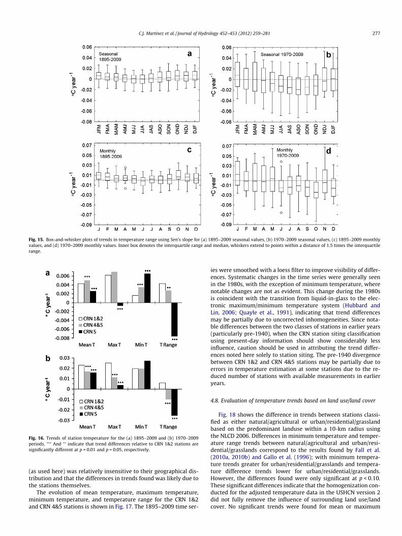
Fig. 15. Box-and-whisker plots of trends in temperature range using Sen’s slope for (a) 1895–2009 seasonal values, (b) 1970–2009 seasonal values, (c) 1895–2009 monthlyvalues, and (d) 1970–2009 monthly values. Inner box denotes the interquartile range and median, whiskers extend to points within a distance of 1.5 times the interquartilerange.

Fig. 16. Trends of station temperature for the (a) 1895–2009 and (b) 1970–2009periods. ⁄⁄⁄ And ⁄⁄ indicate that trend differences relative to CRN 1&2 stations aresignificantly different at p = 0.01 and p = 0.05, respectively.

C.J. Martinez et al. / Journal of Hydrology 452–453 (2012) 259–281 277

(as used here) was relatively insensitive to their geographical dis-tribution and that the differences in trends found was likely due tothe stations themselves.

The evolution of mean temperature, maximum temperature,minimum temperature, and temperature range for the CRN 1&2and CRN 4&5 stations is shown in Fig. 17. The 1895–2009 time ser-

ies were smoothed with a loess filter to improve visibility of differ-ences. Systematic changes in the time series were generally seenin the 1980s, with the exception of minimum temperature, wherenotable changes are not as evident. This change during the 1980sis coincident with the transition from liquid-in-glass to the elec-tronic maximum/minimum temperature system (Hubbard andLin, 2006; Quayle et al., 1991), indicating that trend differencesmay be partially due to uncorrected inhomogeneities. Since nota-ble differences between the two classes of stations in earlier years(particularly pre-1940), when the CRN station siting classificationusing present-day information should show considerably lessinfluence, caution should be used in attributing the trend differ-ences noted here solely to station siting. The pre-1940 divergencebetween CRN 1&2 and CRN 4&5 stations may be partially due toerrors in temperature estimation at some stations due to the re-duced number of stations with available measurements in earlieryears.

4.8. Evaluation of temperature trends based on land use/land cover

Fig. 18 shows the difference in trends between stations classi-fied as either natural/agricultural or urban/residential/grasslandbased on the predominant landuse within a 10-km radius usingthe NLCD 2006. Differences in minimum temperature and temper-ature range trends between natural/agricultural and urban/resi-dential/grasslands correspond to the results found by Fall et al.(2010a, 2010b) and Gallo et al. (1996); with minimum tempera-ture trends greater for urban/residential/grasslands and tempera-ture difference trends lower for urban/residential/grasslands.However, the differences found were only significant at p < 0.10.These significant differences indicate that the homogenization con-ducted for the adjusted temperature data in the USHCN version 2did not fully remove the influence of surrounding land use/landcover. No significant trends were found for mean or maximum

Fig. 17. Time series of annual maximum temperature anomalies for the (a) 1895–2009 and (b) 1970–2009 time periods, mean temperature anomalies for the (c) 1895–2009and (d) 1970–2009 time periods, minimum temperature anomalies for the (e) 1895–2009 and (f) 1970–2009 time periods, and temperature range anomalies for the (g) 1895–2009 and (h) 1970–2009 time periods. 1895–2009 Time series have been smoothed using a loess filter.

278 C.J. Martinez et al. / Journal of Hydrology 452–453 (2012) 259–281

temperature. In particular, the decrease in maximum temperaturetrends found by Karl et al. (1988) was not found in this analysis.However, it has been noted that urbanization has less impact onmaximum temperature and that trends in maximum and mini-mum temperature may cancel each other when mean temperatureis considered (Fall et al., 2011). No significant trends were foundfor the 1895–2009 period (not shown). The results found basedon regional land use/land cover differed than that found basedon station siting since the station siting classification was basedon conditions in the immediate vicinity of the station while theevaluation based on land use/land cover was more regional in

scale. Reclassification of the original 16 classes of the NLCD intomore than two classes (e.g. considering grassland/pasture/scrubas a separate class(es), etc.) were evaluated but no statistical differ-ences were found for either time period. This may be due, in part,to the relatively small sample size used (22 stations). As noted forthe analysis based on station siting classification, the stations clas-sified by regional land use/land cover were irregularly distributedand conclusions should be drawn with caution. It should be notedthat use of only the 2006 land use dataset here does not explicitlyshow the change of landuse that might have occurred nor when itmay have occurred. However, given the relatively low human

Fig. 18. Trends per decade for the 1970–2009 period for the stations classified as natural/agricultural and urban/residential/grassland. ⁄ Indicates significant difference atp < 0.10.

C.J. Martinez et al. / Journal of Hydrology 452–453 (2012) 259–281 279

population in Florida (US Census Bureau, 1995) in the early 20thcentury it can reasonably be assumed that most, if not all of the ur-ban and residential areas, and much of the grassland areas had pre-viously been forest or wetlands (Myers and Ewel, 1990).

5. Conclusion

This work provided a state-level evaluation of historical trendsfor both the period of record of the USHCN version 2 dataset, andrecent years. As found by Karl et al. (1989), changes in precipitationwere less pronounced than those found for temperature. Field sig-nificant and generally increasing trends were found in the JJA sea-son and overall decreasing trends were found for the months ofOctober and May for the 1895–2009 and 1970–2009 periods,respectively. Homogenization of monthly precipitation resultedin similar results in terms of field significance, but with a notablereduction in negative local trends in annual and seasonal precipita-tion but not in monthly. Field significant increases in mean, maxi-mum, and minimum temperature were found in most seasons andmonths of the year. Trends in temperature variables were mostpronounced in terms of the number of seasons/months showing lo-cally significant trends in the west-central and southern portionsof the state.

Trends in temperature range were field significant at all seasonsand months, but were less spatially coherent than those found formean, maximum, and minimum temperature. This may be par-tially due to the compounding effect of trends of different magni-tude in maximum and minimum temperature caused by issuesin station siting, however this work did not find a large prevalenceof opposite signed trends in maximum and minimum temperatureas noted by Fall et al. (2011).

Significant differences in most temperature variables werefound between good and poorly sited stations based on the classi-fication of USHCN stations using the USCRN rating system. No sig-

nificant differences were found for maximum temperature andminimum temperature trends in the 1895–2009 and 1970–2009periods, respectively. This work did not find the cancelation effecton mean temperature due to oppositely signed trends in maximumand minimum temperature as found by Fall et al. (2011) in theirconterminous-wide study using the USHCN dataset, indicating thatmean temperature trends in Florida may be impacted by stationexposure. However, the attribution of trend differences based so-lely on station siting should be done with caution since notable dif-ferences between stations based on their rating were noted pre-1940, a time that the present-day ratings may or may not be valid.Significant differences in temperature trends based on land usewithin a 10-km radius were only found for minimum temperatureand temperature range.

This work provides a preliminary analysis of historical trends inthe climate record in the state of Florida. While this work did notattempt to fully attribute the cause of observed trends, it providesa first step in future attribution to possible causes including multi-decadal climate variability, long term regional temperature trends,and potential errors caused by station siting, regional land use/landcover, and data homogenization.

Acknowledgements

Financial assistance for this project was provided by College ofAgriculture and Life Sciences/Institute of Food and AgriculturalSciences at the University of Florida and the Climate ProgramOffice of the US Department of Commerce, National Oceanic andAtmospheric Administration (NOAA) pursuant to Sector Applica-tions Research Program (SARP) NOAA Award No. NA10OAR4310171. The statements, findings, conclusions, and recommen-dations are those of the research team and do not necessarilyreflect the views of NOAA, US Department of Commerce, or theUS Government.

280 C.J. Martinez et al. / Journal of Hydrology 452–453 (2012) 259–281

References

Alexandersson, A., 1986. A homogeneity test applied to precipitation data. J. Clim. 6,661–675.

Arnell, N.W., Delaney, E.K., 2006. Adapting to climate change: public water supplyin England and Wales. Clim. Change 78 (2), 227–255.

Barsugli, J., Anderson, C., Smith, J.B., Vogel, J.M., 2009. Options for Improving ClimateModeling to Assist Water Utility Planning for Climate Change. White Paper,Water Utility Climate Alliance.

Brekke, L.D., Kiang, J.E., Olsen, J.R., Pulwarty, R.S., Raff, D.A., Turnipseed, D.P., Webb,R.S., White, K.D., 2009. Climate Change and Water Resources Management: AFederal Perspective. US Geological Survey Circular 1331, 65p. <http://pubs.usgs.gov/circ/1331/>.

Bristow, K.L., Campbell, G.S., 1984. On the relationship between incoming solarradiation and daily maximum and minimum temperature. Agr. Forest Meteorol.31, 159–166.

Burn, D.H., Hag Elnur, M.A., 2002. Detection of hydrologic trends and variability. J.Hydrol. 255, 107–122.

Christy, J.R., Norris, W.B., NcNider, R.T., 2009. Surface temperature variations in eastAfrica and possible causes. J. Clim. 22, 3342–3356.

Christy, J.R., Norris, W.B., Redmond, K., Gallo, K.P., 2006. Methodology and results ofcalculating central California surface temperature trends: evidence of humaninduced climate change? J. Clim. 19, 548–563.

Davey, C.A., Pielke Sr., R.A., 2005. Microclimate exposures of surface-based weatherstations. B. Am. Meteor. Soc. 86, 497–504.

Douglas, E.M., Vogel, R.M., Kroll, C.N., 2000. Trends in floods and low flows in theUnited States: impact of spatial correlation. J. Hydrol. 240, 90–105.

Fall, S., Diffenbaugh, N.S., Niyogi, D., Pielke Sr., R.A., Rochon, G., 2010a. Temperatureand equivalent temperature over the United States (1979–2005). Int. J. Climatol.30, 2045–2054.

Fall, S., Niyogi, D., Gluhovsky, A., Pielke Sr., R.A., Kalnay, E., Rochon, G., 2010b.Impacts of land use land cover on temperature trends over the continentalUnited States: assessment using the North American Regional Reanalysis. Int. J.Climatol. 30, 1980–1993.

Fall, S., Watts, A., Nielsen-Gammon, J., Jones, E., Niyogi, D., Christy, J.R., Pielke Sr.,R.A., 2011. Analysis of the impacts of station exposure on the US HistoricalClimatology Network temperatures and temperature trends. J. Geophys. Res.116, D14120. http://dx.doi.org/10.1029/2010JD015146, 2011.

Fry, J., Xian, G., Jin, S., Dewitz, J., Homer, C., Yang, L., Barnes, C., Herold, N., Wickham,J., 2011. Completion of the 2006 national land cover database for theconterminous United States. Photogram. Eng. Remote Sens. 77 (9), 858–864.

Gallo, K.P., Easterling, D.R., Peterson, T.C., 1996. The influence of land use/land coveron climatological values of the diurnal temperature range. J. Clim. 9, 2941–2944.

Guijarro, J.A., 2011. Users guide to climatol. An R contributed package forhomogenization of climatological series. Report to the State MeteorologicalAgency, Balearic Islands Office, Spain. <http://webs.ono.com/climatol/climatol.html>.

Hale, R.C., Gallo, K.P., Loveland, T.R., 2008. Influences of specific land use/land coverconversions on climatological normals of near-surface temperature. J. Geophys.Res. 113, D14113. http://dx.doi.org/10.1029/2007JD009548.

Hamlet, A.F., 2011. Assessing water resources adaptive capacity to climate changeimpacts in the Pacific Northwest region of North America. Hydrol. Earth Syst.Sci. 15, 1427–1443.

Hargreaves, G.H., Samani, Z.A., 1982. Estimating potential evapotranspiration. J.Irrig. Drain. Eng. 108 (IR3), 225–230.

Helsel, D.R., Hirsch, R.M., 2002. Statistical Methods in Water Resources. Techniquesof Water Resources Investigations Book 4, Chapter A3, United States GeologicalSurvey, 552pp. <http://pubs.usgs.gov/twri/twri4a3/>.

Hubbard, K.G., Lin, X., 2006. Reexamination of instrument change effects in the USHistorical Climatology Network. Geophys. Res. Lett. 33, L15710. http://dx.doi.org/10.1029/2006GL027069.

Jensen, M.E., Burman, R.D., Allen, R.G., 1990. Evapotranspiration and IrrigationWater Requirements. ASCE Manuals and Reports on Engineering Practice No.70, American Society of Civil Engineers, New York.

Kalnay, E., Cai, M., 2003. Impact of urbanization and land-use change on climate.Nature 423, 528–531.

Karl, T.R., Williams Jr., C.N., Young, P.J., Wendland, W.M., 1986. A model to estimatethe time of observation bias associated with monthly mean maximum,minimum, and mean temperatures for the United States. J. Clim. Appl.Meteorol. 25, 145–160.

Karl, T.R., Diaz, H.F., Kukla, G., 1988. Urbanization: its detection and effect in theUnited States climate record. B. Am. Meteor. Soc. 69 (11), 1099–1123.

Karl, T.R., Tarpley, J.D., Quayle, R.G., Diaz, H.F., Robinson, D.A., Bradley, R.S., 1989.The recent climate record: what it can and cannot tell us. Rev. Geophys. 27 (3),405–430.

Kendall, M.G., 1975. Rank Correlation Methods. Charles Griffin, London.Khaliq, M.N., Ouarda, T.B.M.J., 2007. On the critical values of the standard normal

homogeneity test. Int. J. Climatol. 27, 681–687.Kunkel, K.E., Andsager, K., Easterling, R.M., 1999. Long-term trends in extreme

precipitation events over the conterminous United States and Canada. J. Clim.12, 2515–2527.

Lettenmaier, D.P., Wood, E.F., Wallis, J.R., 1994. Hydro-climatological trends in theContinental United States, 1948–1988. J. Clim. 7, 586–607.

Livezey, R.E., Chen, W.Y., 1983. Statistical field significance and its determination byMonte Carlo techniques. Mon. Weather Rev. 111, 46–59.

Lobell, D.B., Bonfils, C., 2008. The effect of irrigation on regional temperatures: aspatial and temporal analysis of trends in California, 1934–2002. J. Clim. 21,2064–2071.

Lu, Q., Lund, R., Seymour, L., 2005. An update of US temperature trends. J. Clim. 18,4906–4914.

Mahmood, R., Foster, S.A., Keeling, T., Hubbard, K.G., Carlson, C., Leeper, R., 2006.Impacts of irrigation on 20th-century temperatures in the Northern GreatPlains. Global Planet. Change 54, 1–18.

Mann, H.B., 1945. Non-parametric tests against trend. Econometrica 13 (3), 245–259.

Marshall, C.H., Pielke Sr., R.A., Steyaert, L.T., 2004a. Has the conversion of naturalwetlands to agricultural land increased the incidence and severity of damagingfreezes in south Florida? Mon. Weather Rev. 132, 2243–2258.

Marshall, C.H., Pielke Sr., R.A., Steyaert, L.T., Willard, D.A., 2004b. The impact ofanthropogenic land-cover change on the Florida peninsula sea breezes andwarm season sensible weather. Mon. Weather Rev. 132, 28–52.

Menne, M.J., Williams Jr., C.N., 2009. Homogenization of temperature series viapairwise comparisons. J. Clim. 22, 1700–1717.

Menne, M.J., Williams Jr., C.N., Palecki, M.A., 2010. On the reliability of the USsurface temperature record. J. Geophys. Res. 115, D11108. http://dx.doi.org/10.1029/2009JD013094, 2010.

Menne, M.J., Williams Jr., C.N., Vose, R.S., 2009. The US historical climatologynetwork monthly temperature data, version 2. B. Am. Meteor. Soc. 90 (7), 993–1007.

Menne, M.J., Williams Jr., C.N., Vose, R.S., 2011. United States Historical ClimatologyNetwork (USHCN) Version 2 Serial Monthly Dataset. Carbon DioxideInformation Analysis Center, Oak Ridge National Laboratory, Oak Ridge,Tennessee.

Mishra, V., Lettenmaier, D.P., 2011. Climatic trends in major US urban areas, 1950–2009. Geophys. Res. Lett. 38, L16401. http://dx.doi.org/10.1029/2011GL048255,2011.

Myers, R.L., Ewel, J.J., 1990. Ecosystems of Florida. University of Central FloridaPress, Orlando, FL, 765pp.

National Oceanic and Atmospheric Administration and National EnvironmentalSatellite, Data, and Information Service (NOAA and NESDIS), 2002. ClimateReference Network Site Information Handbook. NOAA-CRN/OSD-2002-0002ROUD0, United States Department of Commerce, 29pp.

National Research Council (NRC), 2005. Radiative Forcing of Climate Change:Expanding the Concept and Addressing Uncertainties. The National AcademiesPress, Washington, DC. 208pp.

Peterson, T.C., Owen, T.W., 2005. Urban heat island assessment: Metadeta areimportant. J. Clim. 18, 2637–2646.

Peterson, T.C., Willett, K.M., Thorne, P.W., 2011. Observed changes in surfaceatmospheric energy over land. Geophys. Res. Lett. 38, L16707. http://dx.doi.org/10.1029/2011GL048442.

Pielke Sr., R., Nielsen-Gammon, J., Davey, C., Angel, J., Bliss, O., Doesken, N., Cai, M.,Fall, S., Niyogi, D., Gallo, K., Hale, R., Hubbard, K.G., Lin, X., Li, H., Raman, S., 2007.Documentation of uncertainties and biases associated with surface temperaturemeasurement sites for climate change assessment. B. Am. Meteor. Soc. 88, 913–928.

Pielke Sr., R.A., Walko, R.L., Steyart, L.T., Vidale, P.L., Liston, G.E., Lyons, W.A., Chase,T.N., 1999. The influence of anthropogenic landscape changes on weather insouth Florida. Mon. Weather Rev. 127 (7), 1663–1673.

Quayle, R.G., Easterling, D.R., Karl, T.R., Hughes, P.Y., 1991. Effects of recentthermometer changes in the Cooperative Station Network. B. Am. Meteor. Soc.72, 1718–1723.

R Development Core Team, 2011. R: A Language and Environment for StatisticalComputing. R Foundation for Statistical Computing, Vienna, Austria. <http://www.R-project.org>.

Raucher, R.S. 2011. The Future of Research on Climate Change Impacts on Water: AWorkshop Focused on Adaption Strategies and Information Needs. WaterResearch Foundation. <http://www.waterrf.org/projectsreports/publicreportlibrary/4340.pdf>.

Rosenzweig, C., Major, D.C., Demong, K., Stanton, C., Horton, R., Stults, M., 2007.Managing climate change risks in New York City’s water system: assessmentand adaptation planning. Mitig. Adapt. Strat. Global Change 12 (8), 1391–1409.

Roy, S.S., Mahmood, R., Niyogi, D., Lei, M., Foster, S.A., Hubbard, K.G., Douglas, E.,Pielke Sr., R.A., 2007. Impacts of the agricultural green revolution – induced landuse changes on air temperatures in India. Geophys. Res. 112, D21108. http://dx.doi.org/10.1029/2007JD008834.

Runnalls, K.E., Oke, T.R., 2006. A technique to detect microclimate inhomogeneitiesin historical records of screen-level air temperature. J. Clim. 19, 959–978.

Sen, P.K., 1968. Estimates of the regression coefficient based on Kendall’s tau. J. Am.Stat. Assoc. 63, 1379–1389.

Suppiah, R., Hennessy, K.J., 1998. Trends in total rainfall, heavy rain events andnumber of dry days in Australia, 1910–1990. Int. J. Climatol. 10, 1141–1164.

United States Census Bureau, 1995. Florida Population of Counties by DecennialCensus: 1900–1990. Compiled and edited by R.L. Forstall. <http://www.census.gov/population/cencounts/fl190090.txt>. (retrieved 6.04.12).

Venema, V.K.C., Mestre, O., Aguilar, E., Auer, I., Guijarro, J.A., Domonkos, P.,Vertacnik, G., Szentimrey, T., Stepanek, P., Zahradnicek, P., Viarre, J., Müller-Westermeier, G., Lakatos, M., Williams, C.N., Menne, M.J., Lindau, R., Rasol, D.,Rustemeier, E., Kolokythas, K., Marinova, T., Andresen, L., Acquaotta, F.,Fratianni, S., Cheval, S., Klancar, M., Brunetti, M., Gruber, C., Prohom Duran,

C.J. Martinez et al. / Journal of Hydrology 452–453 (2012) 259–281 281

M., Likso, T., Esteban, P., Brandsma, T., 2005. Benchmarking homogenizationalgorithms for monthly data. Clim. Past 8, 89–115.

Vose, R.S., Williams Jr., C.N., Peterson, T.C., Karl, T.R., Easterling, D.R., 2003. Anevaluation of the time of observation bias adjustment in the US HistoricalClimatology Network. Geophys. Res. Lett. 30, 2046. http://dx.doi.org/10.1029/2003GL018111.

Watts, A., 2009. Is the US Surface Temperature Record Reliable? Heartland Institute,Chicago, IL, 28pp.

Wilks, D.S., 1996. Statistical significance of long-range ‘‘optimal climate normal’’temperature and precipitation forecasts. J. Clim. 9, 827–839.

Wilks, D.S., 2006. Statistical Methods in the Atmospheric Sciences. Academic Press,Second Edition, 627pp.

Zolina, O., Simmer, C., Kapala, A., Gulev, S., 2005. On the robustness of the estimatesof centennial-scale variability in heavy precipitation from station dataover Europe. Geophys. Res. Lett. 32, L14707. http://dx.doi.org/10.1029/2005GL023231.