journal of monetary economics - columbia universitysn2294/pub/jme10.pdfdistinct is that they consist...
TRANSCRIPT

Estimation of DSGE models when the data are persistent$
Yuriy Gorodnichenko a,!, Serena Ng b
a Department of Economics, University of California, Berkeley, NBER, and IZA, USAb Department of Economics, Columbia University, USA
a r t i c l e i n f o
Article history:Received 9 October 2007Received in revised form17 February 2010Accepted 19 February 2010Available online 6 March 2010
JEL classification:C32C5E32
Keywords:Persistent dataFiltersTrendsUnit rootSpurious estimatesBusiness cycles
a b s t r a c t
Dynamic stochastic general equilibrium (DSGE) models are often solved and estimatedunder specific assumptions as to whether the exogenous variables are difference ortrend stationary. However, even mild departures of the data generating process fromthese assumptions can severely bias the estimates of the model parameters. This paperproposes new estimators that do not require researchers to take a stand on whethershocks have permanent or transitory effects. These procedures have two key features.First, the same filter is applied to both the data and the model variables. Second, thefiltered variables are stationary when evaluated at the true parameter vector. Theestimators are approximately normally distributed not only when the shocks are mildlypersistent, but also when they have near or exact unit roots. Simulations show thatthese robust estimators perform well especially when the shocks are highly persistentyet stationary. In such cases, linear detrending and first differencing are shown to yieldbiased or imprecise estimates.
& 2010 Elsevier B.V. All rights reserved.
1. Introduction
Dynamic stochastic general equilibrium (DSGE) models are now accepted as the primary framework for macroeconomicanalysis. Until recently, counterfactual experiments were conducted by assigning the parameters of the models with valuesthat are loosely calibrated to the data. More recently, serious efforts have been made to estimate the model parametersusing classical and Bayesian methods. This permits researchers to assess how well the models fit the data both in and outof samples. Formal estimation also permits errors arising from sampling or model uncertainty to be explicitly accountedfor in counterfactual policy simulations. Arguably, DSGE models are now taken more seriously as a tool for policy analysisbecause of such serious econometric investigations.
Any attempt to estimate DSGE models must confront the fact that macroeconomic data are highly persistent. This factoften requires researchers to take a stand on the specification of the trends in DSGE models. Specifically, to take the modelto the data, a researcher needs to use sample analogs of the deviations from steady states and, in doing so, must decidehow to detrend the variables in the model and in the data. Table 1 is a non-exhaustive listing of how trends are treated in
Contents lists available at ScienceDirect
journal homepage: www.elsevier.com/locate/jme
Journal of Monetary Economics
ARTICLE IN PRESS
0304-3932/$ - see front matter & 2010 Elsevier B.V. All rights reserved.doi:10.1016/j.jmoneco.2010.02.008
$ This paper was presented at Brown University, the University of Michigan, the 2007 NBER Summer Institute, Princeton University, UC Berkeley, andthe New York Area Macro Conference. We thank Marc Giannone, Tim Cogley, Anna Mikusheva, and two anonymous referees, the Associate Editor and theEditor for many helpful comments. The second author acknowledges financial support from the National Science Foundation (SES 0549978).! Corresponding author.E-mail address: [email protected] (Y. Gorodnichenko).
Journal of Monetary Economics 57 (2010) 325–340

some notable papers.1 Some studies assume stochastic trends for the model and use first differenced data in estimation. Anumber of studies specify deterministic trends for the model and use linearly detrended data in estimation. Studies thatapply the Hodrick–Prescott (HP) filter to the data differ in what trends are specified for the model. Some assume simplelinear trends, while others assume unit root processes. Table 1 demonstrates that a variety of trends have been specifiedfor the model and a variety of detrending methods have been used in estimation.
The problem for researchers is that it is not easy to ascertain whether highly persistent data are trend stationaryor difference stationary in finite samples. While many have studied the implications for estimation and inferenceof inappropriate detrending in linear models,2 much less is known about the effects of detrending in estimation of non-linearmodels. From simulation evidence of Doorn (2006) for an inventory model, it seems that HP filtering can significantlybias the estimated dynamic parameters. While the local-to-unit framework is available to help researchers understand theproperties of the estimated autoregressive root when the data are strongly persistent, it is unclear to what extent theframework can be used in non-linear estimation even in the single equation case. What makes estimation of DSGE modelsdistinct is that they consist of a system of equations and misspecification in one equation can affect estimates in otherequations.
This paper develops robust estimation procedures that do not require researchers to take a stand on whether shocks inthe model have an exact or a near unit root, and yet obtain consistent estimates of the model parameters. All robustprocedures have two characteristics. First, the same transformation (filter) is applied to both the data and the modelvariables. Second, the filtered variables are stationary when evaluated at the true parameter vector. The estimators havethe classical properties of being
!!!T
pconsistent and asymptotically normal for all values of the largest autoregressive root.
Our point of departure is that the rather common practice of applying different filters to the model variables and the datacan have undesirable consequences. As will be shown later, estimates of parameters governing the propagation andamplification mechanisms in the model can be severely distorted when the trend specified for the model is not consistentwith the one applied to the data. We insist on estimators that apply the same transformation to both the model and the data.This, however, may still lead to biased estimates if the filter does not remove the trends actually present in the data.Accordingly, one needs to work with filters that can remove both deterministic and stochastic trends without the researcher
ARTICLE IN PRESS
Table 1Summary of selected work.
Paper Equations Forcing variable Model filter Data filter Estimator
Kydland and Prescott (1982) System ARMA(1,1) LT HP CalibrationAltug (1989) System I(1) FD1 FD1 MLEChristiano and Eichenbaum (1992) System I(1) zt HP GMMBurnside et al. (1993) System AR(1) LT HP GMMBurnside and Eichenbaum (1996) System I(1) zt HP GMMMcGrattan et al. (1997) System VAR(2) LT LT,HP MLEFuhrer (1997) Equation Not specified Not specified HP,LT,QT GMMClarida et al. (2000) Equation AR(1) Not specified LT,HP,CBO GMMKim (2000) System AR(1) LT LT MLEIreland (2001) System AR(1) LT LT MLESmets and Wouters (2003) System AR(1) LT HP BayesianDib (2003) System AR(1) LT LT MLEFuhrer and Rudebusch (2004) Equation Not specified Not specified HP,CBO,QT MLE,GMMLubik and Schorfheide (2004) System AR(1) LT HP,LT BayesianAltig et al. (2004) System ARI(1,1) FD1 FD1 GMMIreland (2004) System I(1) FD1 FD1 MLEBouakez et al. (2005) System AR(1) LT LT MLEChristiano et al. (2005) System Not specified Not specified VAR GMMDel Negro et al. (2007) System ARI(1,1) FD1 FD1 BayesianFaia (2007) System AR(1) LT HP CalibrationSmets and Wouters (2007) System AR(1) FD FD Bayesian
Note: CBO denotes actual series minus the Congress Budget Office’s measure of potential output. I(1) and ARI(1,1) denote forcing variables with stochastictrends. AR and ARMA denote trend stationary forcing variables. VAR denotes filtering with a vector autoregression which can accommodate trend anddifference stationary processes. FD is first differencing, FD1 is first differencing with the restriction that the forcing variable has a unit root (e.g., rz ! 1), LTis projection on linear time trend, QT is projection on quadratic time trend, HP is Hodrick–Prescott filter, zt is detrending by the level of technology. Thesecond column shows whether a paper estimates a system of equations (‘‘system’’) or a single structural equation (‘‘equation’’).
1 As of June 2009, these papers were cited almost 2500 times at the Web of Science (former Social Science Citation Index) and almost 8000 times atGoogle Scholar.
2 For example, Nelson and Kang (1981) showed that linear detrending a unit root process can generate spurious cycles. Cogley and Nason (1995a)found that improper filtering can alter the persistence and the volatility of the series while spurious correlations in the filtered data was documented inHarvey and Jaeger (1993). Singleton (1988) and Christiano and den Haan (1996) discussed how inappropriate filtering can affect estimation and inferencein linear models.
Y. Gorodnichenko, S. Ng / Journal of Monetary Economics 57 (2010) 325–340326
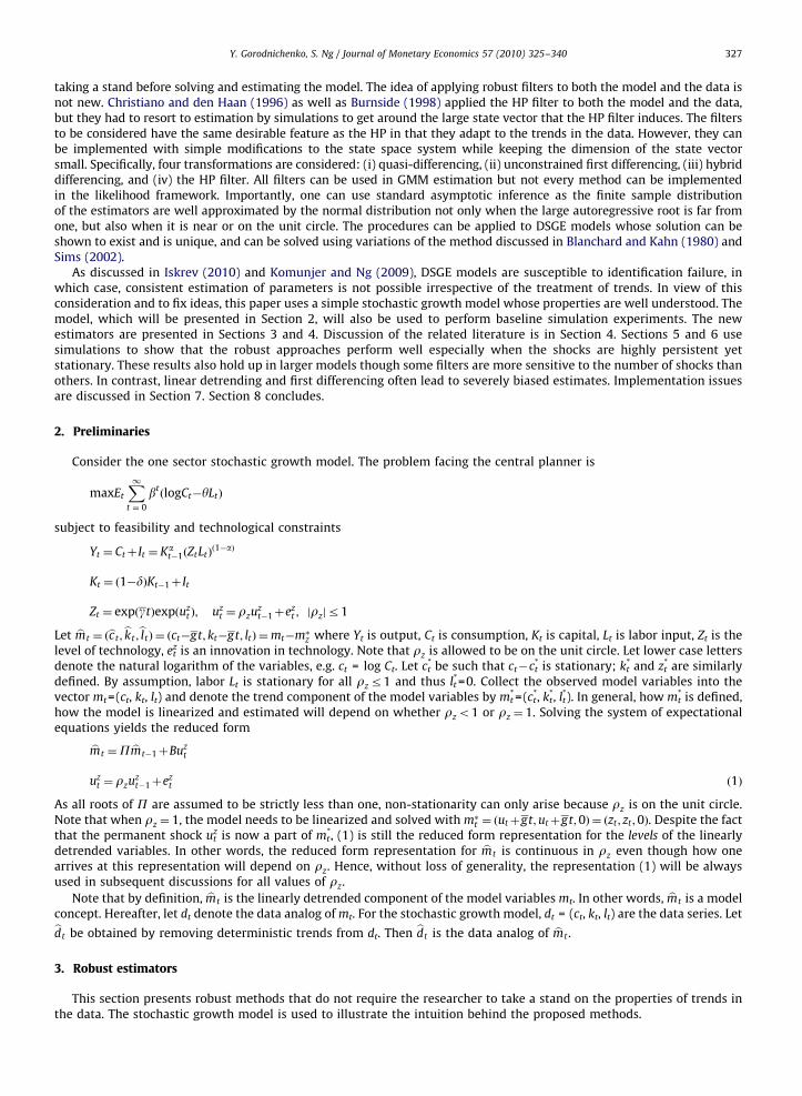
taking a stand before solving and estimating the model. The idea of applying robust filters to both the model and the data isnot new. Christiano and den Haan (1996) as well as Burnside (1998) applied the HP filter to both the model and the data,but they had to resort to estimation by simulations to get around the large state vector that the HP filter induces. The filtersto be considered have the same desirable feature as the HP in that they adapt to the trends in the data. However, they canbe implemented with simple modifications to the state space system while keeping the dimension of the state vectorsmall. Specifically, four transformations are considered: (i) quasi-differencing, (ii) unconstrained first differencing, (iii) hybriddifferencing, and (iv) the HP filter. All filters can be used in GMM estimation but not every method can be implementedin the likelihood framework. Importantly, one can use standard asymptotic inference as the finite sample distributionof the estimators are well approximated by the normal distribution not only when the large autoregressive root is far fromone, but also when it is near or on the unit circle. The procedures can be applied to DSGE models whose solution can beshown to exist and is unique, and can be solved using variations of the method discussed in Blanchard and Kahn (1980) andSims (2002).
As discussed in Iskrev (2010) and Komunjer and Ng (2009), DSGE models are susceptible to identification failure, inwhich case, consistent estimation of parameters is not possible irrespective of the treatment of trends. In view of thisconsideration and to fix ideas, this paper uses a simple stochastic growth model whose properties are well understood. Themodel, which will be presented in Section 2, will also be used to perform baseline simulation experiments. The newestimators are presented in Sections 3 and 4. Discussion of the related literature is in Section 4. Sections 5 and 6 usesimulations to show that the robust approaches perform well especially when the shocks are highly persistent yetstationary. These results also hold up in larger models though some filters are more sensitive to the number of shocks thanothers. In contrast, linear detrending and first differencing often lead to severely biased estimates. Implementation issuesare discussed in Section 7. Section 8 concludes.
2. Preliminaries
Consider the one sector stochastic growth model. The problem facing the central planner is
maxEtX1
t ! 0
bt"logCt#yLt$
subject to feasibility and technological constraints
Yt ! Ct% It ! Kat#1"ZtLt$
"1#a$
Kt ! "1#d$Kt#1% It
Zt ! exp"gt$exp"uzt $; uz
t ! rzuzt#1%ezt ; jrzjr1
Let bmt ! "bct ; bkt ;blt$ ! "ct#gt; kt#gt; lt$ !mt#m&z where Yt is output, Ct is consumption, Kt is capital, Lt is labor input, Zt is the
level of technology, ezt is an innovation in technology. Note that rz is allowed to be on the unit circle. Let lower case lettersdenote the natural logarithm of the variables, e.g. ct = log Ct. Let c
*t be such that ct#c*t is stationary; k
*t and z*t are similarly
defined. By assumption, labor Lt is stationary for all rzr1 and thus l*t=0. Collect the observed model variables into thevector mt=(ct, kt, lt) and denote the trend component of the model variables by m*
t=(c*t, k
*t, l
*t). In general, how m*
t is defined,how the model is linearized and estimated will depend on whether rzo1 or rz ! 1. Solving the system of expectationalequations yields the reduced form
bmt !P bmt#1%Buzt
uzt ! rzu
zt#1%ezt "1$
As all roots of P are assumed to be strictly less than one, non-stationarity can only arise because rz is on the unit circle.Note that when rz ! 1, the model needs to be linearized and solved with m&
t ! "ut%gt;ut%gt;0$ ! "zt ; zt ;0$. Despite the factthat the permanent shock uzt is now a part of mt
*, (1) is still the reduced form representation for the levels of the linearlydetrended variables. In other words, the reduced form representation for bmt is continuous in rz even though how onearrives at this representation will depend on rz. Hence, without loss of generality, the representation (1) will be alwaysused in subsequent discussions for all values of rz.
Note that by definition, bmt is the linearly detrended component of the model variablesmt. In other words, bmt is a modelconcept. Hereafter, let dt denote the data analog ofmt. For the stochastic growth model, dt = (ct, kt, lt) are the data series. Letbdt be obtained by removing deterministic trends from dt. Then bdt is the data analog of bmt .
3. Robust estimators
This section presents robust methods that do not require the researcher to take a stand on the properties of trends inthe data. The stochastic growth model is used to illustrate the intuition behind the proposed methods.
ARTICLE IN PRESSY. Gorodnichenko, S. Ng / Journal of Monetary Economics 57 (2010) 325–340 327

Many methods have been used to estimate DSGE models.3 Our focus will be a method of moments (MM) estimator thatminimizes the distance between the second moments of data and the second moments implied by the model, as inChristiano and den Haan (1996) and Christiano and Eichenbaum (1992). Adaptation to likelihood based estimation will bediscussed in Section 7.
Let Y denote the unknown structural parameters of the model and partition Y! "Y#;rz$. The generical MM estimator
can be summarized as follows. Step 1 applies a filter (if necessary) to dt and computes bOd"j$, the estimated covariance
matrix of the filtered series at lag j. Collect the data moments in the vector
bod ! "vech"bOd"0$$0 vec"bO
d"1$$0 . . .vec"bO
d"M$$0$0
Step 2 solves the rational expectations model for a guess of Y. Compute Om"j$, the model implied autocovariances of the
filtered bmt analytically or by simulation. Collect the model moments in the vector
om ! "vech"Om"0$$0 vec"Om"1$$0 . . .vec"Om"M$$0$0
Step 3 estimates the structural parameters as
bY ! argminY
J bod#om"Y$J
The choice of moments in MM can be important for identification (see e.g. Canova and Sala, 2009). The unconditionalautocovariances are used in this paper but matching impulse responses can also be considered. Although MM is somewhatless widely used than maximum likelihood estimators in the DSGE literature, it does not require parametric specification ofthe error processes and it is easy to implement. As will be discussed later, the more important reason for using MM ispractical as it can be used with many popular filters.
The robust approaches considered here always apply the same filter to the model and the data so that the filteredvariables are stationary when evaluated at the true parameter of rz, which can be one or close to one. The statisticalproperties of bY will depend on rz and the filters used. The next four subsections consider four filters. Section 4 thenexplores which of these have better finite samples properties. Properties of estimators that do not have these features willalso be compared later.
3.1. The QD estimator
Let Drz ! 1#rzL be the quasi-differencing (QD) operator and let Drz bmt ! "1#rzL$ bmt . Multiplying both sides of (1) by Drz
and using uzt ! rzu
zt#1%ezt gives
Drz bmt !PDrz bmt#1%Bezt "2$
Note that the error term in the quasi-differenced model is an i.i.d. innovation. As Drz bmt is stationary for all rzr1, itsmoments are well defined. In contrast, the moments of bmt are not well defined when rz ! 1. This motivates estimation ofY as follows.
First, initialize rz. Second, quasi-differencebdt with rz to obtain Drzbdt . Compute bO
d
Drz "j$ ! cov"Drzbdt ;Drzbdt#j$; the sample
autocovariance matrix of the quasi-differenced data at lag j! 0; . . . ;M. Define bUd
Drz "j$ ! bOd
Drz "j$#bOd
Drz "0$ and let
bodDrz ! "vec"bU
d
Drz "1$$0; . . . ;vec"bUd
Drz "M$$0$0. Third, for a given rz and Y#, solve for the reduced form (1). Apply Drz to bmt
and compute OmDrz "j$; j! 1; . . . ;M, the model implied autocovariance matrices of the quasi-differenced variables. Let
UmDrz "j$ !Om
Drz "j$#OmDrz "0$. Define om
Drz "rz$ ! "vec"UmDrz "1$$0; . . . ;vec"Um
Drz "M$$0$0. Fourth, find the structural parameters
bYQD ! argminYJ bodDrz "rz$#om
Drz "Y$J.The QD estimator is based on the difference between the model and the sample autocovariances of the filtered
variables, normalized by the respective variance matrixODrz "0$. The QD differs from a standard covariance estimator in oneimportant respect. The parameter rz now affects both the moments of the model and the data since the latter arecomputed for the data quasi-differenced at rz. As rz and Y# are estimated simultaneously, the filter is data dependentrather than fixed. The crucial feature is that the quasi-transformed data are stationary when evaluated at the true rz, whichsubsequently permits application of a central limit theorem. The normalization of the lagged autocovariances by thevariance amounts to using the moments
cov"Drzbdt ;Drzbdt#Drzbdt#j$#cov"Drz bmt ;Drz bmt#Drz bmt#j$
for estimation. The j-th difference of Drzbdt is always stationary and ensures that the asymptotic distribution is wellbehaved. Finally, observe that since the model is solved in levels and the transformed variables are used only to computemoments, all equilibrium relationships between variables are preserved.
ARTICLE IN PRESS
3 This includes likelihood and Bayesian based methods (e.g. Fernandez-Villaverde and Rubio-Ramirez, 2007; Ireland, 1997), two-step minimumdistance approach (e.g., Sbordone, 2006), as well as simulation estimation (e.g., Altig et al., 2004). Ruge-Murcia (2007) provides a review of these methods.
Y. Gorodnichenko, S. Ng / Journal of Monetary Economics 57 (2010) 325–340328

3.2. The FD estimator
If Drz bmt is stationary when rzr1, the data vector is also stationary when quasi-differenced at rz ! 1. Denote the first-differencing (FD) operator by D! 1#L and consider the following estimation procedure. First, compute
bOd
D"j$ ! cov"Dbdt ;Dbdt#j$, the sample autocovariance matrix of the first differenced data at lag j! 1; . . . ;M. Define
bodD ! "vech"bO
d
D"1$$0; . . . ;vec"bO
d
D"M$$0$0. Second, for a given Y, solve for the reduced form (1). Compute OmD "j$, the model
implied autocovariance matrices of the first-differenced variables D bmt . Define omD ! "vech"Om
D "0$$0; . . . ;vec"Om
D "M$$0$0. Third,
find the structural parameters bYFD ! argminYJ bodD#om
D "Y$J.To be clear, the autocovariances are computed for the first differenced data and the model variables, but rz is a free
parameter which is estimated. Note that the QD and FD estimators are equivalent when rz ! 1. The key difference betweenFD and QD is that FD is a fixed filter while the QD is a data dependent filter.
3.3. The hybrid estimator
One drawback of the FD estimator is that when rz is far from unity, over-differencing induces a non-invertible moving-average component. The estimates obtained by matching a small number of lagged autocovariances may be inefficient. The
QD estimator does not have this problem, but bOd
Drz "j$ is quadratic in rz. As will be explained below, this is why bOd
Drz "j$ was
normalized by bOd
Drz "0$. These considerations suggest a hybrid (HD) estimator.
First, transform the observed data to obtain Drzbdt (as in QD) and Dbdt (as in FD). Second, compute
bOd
QD;D"j$ ! cov"Drzbdt ;Dbdt#j$. Define bodQD;D ! "vec"bO
d
QD;D"0$$0; . . . ;vec"bO
d
QD;D"M$$0$0. Third, for a given Y, solve for the reduced
form (1), and compute the model implied autocovariances between the quasi-differenced and the first differenced
variables. Define omQD;D ! "vec"Om
QD;D"0$$0; . . . ;vec"Om
QD;D"M$$0$0. Fourth, find the structural parameters bYHD !
argminYJ bodQD;D"rz$#om
QD;D"Y$J. Notice that bOd
QD;D"j$ is now linear in rz, unlikebOd
Drz "j$.
3.4. The HP estimator
Linear filters such as the HP and the bandpass can also remove deterministic and stochastic trends, see Baxter and King(1999) and King and Rebelo (1993). The HP detrended series is defined as
HP"L$dt !l"1#L$2"1#L#1$2
1%l"1#L$2"1#L#1$2dt
The estimator can be constructed as follows. First, compute the autocovariance matrices of the HP-filtered data
bOd
HP"0$; . . . ; bOd
HP"M$. Define bodHP ! "vech"bO
d
HP"0$$0; . . . ;vec"bO
d
HP"M$$0$0. Second, for a given guess of Y, solve for the reduced
form (1), and compute Om"j$, the autocovariances of bmt . Apply the Fourier transform to obtain the spectrum for bmt atfrequencies 2ps=T, s! 0; . . . ; T#1. Multiply the spectrum by the gain of the HP filter. Inverse Fourier transform to obtain
OHP"j$, the autocovariances of the HP(L) bmt . Define omHP ! "vech"Om
HP"0$$0; . . . ;vec"Om
HP"M$$0$0. Third, find the structural
parameters bYHP ! argminY: bodHP#om
HP"Y$:.This approach is similar to Burnside (1998) who also first applies the HP filter to both the model and the data series, and
then uses simulations to compute model-implied moments. Like the FD, rz does not enter the filter but both the filtereddata and the filtered model variables are stationary for all rzr1. Note that HP filtering involves estimation of many moreautocovariances than the other estimators considered above.
4. Properties of the estimators
Let bodj generically denote the j-th samplemoments of the filtered variables whileom
j "Y$ denote the model moment based
on the same filter. Define gj"Y$ ! bodj #om
j "Y$ and let g"Y$ ! "g0"Y$; g1"Y$; . . . ; gM"Y$$. Then the MM estimator
bY !minYJg"Y$J is a non-linear GMM estimator using an identity weighting matrix. This sub-optimal weighting matrix isused because when there are fewer shocks than variables in the system, stochastic singularity will induce collinearity in thevariables resulting in a matrix of covariances that would be singular. Even if there are as many shocks as endogenousvariables, Abowd and Card (1989), Altonji and Segal (1996) and others find that an identity matrix performs better than theoptimal weighting matrix in the context of estimating covariance structures. The optimal weighting matrix, which containshigh order moments, tends to correlate with the moments and this correlation undermines the performance of the estimator.
Let G"Y$ be the matrix of derivatives of g"Y$ with respect to Y. In standard covariance structure estimation, theparameters enter the model moments om"Y$ but not the sample bod
, so that if bodare moments of stationary variables,
ARTICLE IN PRESSY. Gorodnichenko, S. Ng / Journal of Monetary Economics 57 (2010) 325–340 329
then under regularity conditions such as stated in Newey and McFadden (1994), the conventional result that bY isconsistent obtains. Furthermore,
!!!T
p" bY#Y0$#!
dA ' N"0; S$
where A! "G00G0$#1G0
0,!!!T
pg"Y0$#!
dN"0; S$, and G0 is the probability limit of G"Y$ evaluated at Y!Y0. This distribution
theory applies to the FD and the HP because these two filters do not depend on unknown parameters and the filtered
variables are always stationary. For the HD estimator, boddepends on rz but its first derivative does not, so that a quadratic
expansion of the objective function can still be used to derive the asymptotic distribution of the estimator. Although G"Y$
for the HD has a random limit when rz ! 1, bodis a vector of covariances of stationary variables when evaluated at the true
value of rz. Thus, the ‘standardized’ HD estimator (or the t statistic) remains asymptotically normal.To understand the properties of the QD estimator, an explanation for why the lagged autocovariances are normalized by
the variance is necessary. Suppose ~gj"Y$ ! bOd
Drz "j$#OmDrz "j$ was used instead of gj"Y$ ! bod
Drz "j$#omDrz "j$ where
odDrz "j$ ! bO
d
Drz "j$#bOd
Drz "0$, and omDrz is likewise defined. Minimizing J ~g "Y$J over Y yields an estimator, say, QD0. The
problem here is that bOd
Drz "j$ is a cross-product of data quasi-differenced at rz, and is thus quadratic in rz. The quadraticexpansion of J ~g"Y$J around Y0 contains terms that are not negligible when rz is one. As such, the sample objectivefunction cannot be shown to converge uniformly to the population objective function. Gorodnichenko et al. (2009) show ina simpler setting that the QD0 estimator for rz is consistent but it has a convergence rate of T3/4 and is not asymptotically
normal. The QD estimator is motivated by the fact that the offending term in the quadratic expansion of bOd
Drz "j$ is collinear
with bOd
Drz "0$ when rz ! 1.
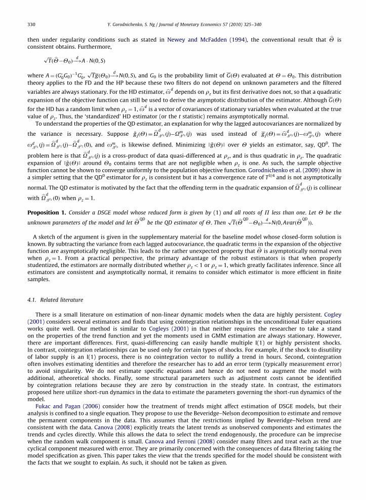
Proposition 1. Consider a DSGE model whose reduced form is given by (1) and all roots of P less than one. Let Y be the
unknown parameters of the model and let bYQD
be the QD estimator of Y. Then!!!T
p" bY
QD#Y0$#!
dN"0;Avar" bY
QD$$.
A sketch of the argument is given in the supplementary material for the baseline model whose closed-form solution isknown. By subtracting the variance from each lagged autocovariance, the quadratic terms in the expansion of the objectivefunction are asymptotically negligible. This leads to the rather unexpected property that bY is asymptotically normal evenwhen rz ! 1. From a practical perspective, the primary advantage of the robust estimators is that when properlystudentized, the estimators are normally distributed whether rzo1 or rz ! 1, which greatly facilitates inference. Since allestimators are consistent and asymptotically normal, it remains to consider which estimator is more efficient in finitesamples.
4.1. Related literature
There is a small literature on estimation of non-linear dynamic models when the data are highly persistent. Cogley(2001) considers several estimators and finds that using cointegration relationships in the unconditional Euler equationsworks quite well. Our method is similar to Cogleys (2001) in that neither requires the researcher to take a standon the properties of the trend function and yet the moments used in GMM estimation are always stationary. However,there are important differences. First, quasi-differencing can easily handle multiple I(1) or highly persistent shocks.In contrast, cointegration relationships can be used only for certain types of shocks. For example, if the shock to disutilityof labor supply is an I(1) process, there is no cointegration vector to nullify a trend in hours. Second, cointegrationoften involves estimating identities and therefore the researcher has to add an error term (typically measurement error)to avoid singularity. We do not estimate specific equations and hence do not need to augment the model withadditional, atheoretical shocks. Finally, some structural parameters such as adjustment costs cannot be identifiedby cointegration relations because they are zero by construction in the steady state. In contrast, the estimatorsproposed here utilize short-run dynamics in the data to estimate the parameters governing the short-run dynamics of themodel.
Fukac and Pagan (2006) consider how the treatment of trends might affect estimation of DSGE models, but theiranalysis is confined to a single equation. They propose to use the Beveridge–Nelson decomposition to estimate and removethe permanent components in the data. This assumes that the restrictions implied by Beveridge–Nelson trend areconsistent with the data. Canova (2008) explicitly treats the latent trends as unobserved components and estimates thetrends and cycles directly. While this allows the data to select the trend endogenously, the procedure can be imprecisewhen the random walk component is small. Canova and Ferroni (2008) consider many filters and treat each as the truecyclical component measured with error. They are primarily concerned with the consequences of data filtering taking themodel specification as given. This paper takes the view that the trends specified for the model should be consistent withthe facts that we sought to explain. As such, it should not be taken as given.
ARTICLE IN PRESSY. Gorodnichenko, S. Ng / Journal of Monetary Economics 57 (2010) 325–340330

5. Simulations: baseline model
This section uses the stochastic growth model to conduct Monte Carlo experiments. Data are generated with eitherdeterministic trends "rzo1$ or stochastic trends "rz ! 1$ using the model equations for bmt . The model variables are thenrescaled back to level form and treated as observed data dt=(ct, kt,yt, lt), which are taken as given in estimation. Thevariance and the first order (M=1) auto- and cross variance of the four variables are used as moments. Alternative choicesof observed variables, such as excluding the capital stock series, yield very similar results.
The model is calibrated as follows: capital intensity a! 0:33; disutility of labor y! 1; discount factor b! 0:99;depreciation rate d! 0:1; gross growth rate in technology g ! 0:005. There is only one shock in this baseline model. Thus,the standard deviation of ezt is set to sz ! 1 without loss of generality. The admissible range of the estimates of a is[0.01,0.99]. The persistence parameter rz takes values (0.95, 0.99, 1). To decouple the treatment of trends from theidentification issues, the parameter vector Y! "a;r;s$ is estimated while "b; d; y$ is assumed known.4 In each of the 2000replications for each parameter set, series with T=200 observations are created. Other sample sizes are also considered.
In all simulations and for all estimators, the starting values in optimization routines are equal to the true parametervalues. The model is solved using the Anderson and Moore (1985) algorithm. Mildly explosive estimates are allowedbecause otherwise solutions for brz will be truncated to the right at one making the distribution of brz highly skewed. Onlyparameter values consistent with a unique rational expectations equilibrium are allowed.5
Table 2 reports simulation results for the baseline growth model. The persistence of technology shocks is given inthe left column. The first and second rows indicate which filter is applied to both the data and the model variables.Columns (1)–(4) report results for the four estimators. By and large, all four filters yield estimates which are very close tothe true values. Notice that while rz is always precisely estimated, the variance of the estimates varies substantially acrossfilters. The QD estimates have the lowest standard deviation while the HP estimates are two to five times more variablethan the QD. The HD is more precise than the FD but is less precise than the QD. This pattern is recurrent in all simulations.
Fig. 1 shows the root mean squared error (RMSE) for different estimators and sample sizes. The QD estimator performsthe best while the FD tends to have the largest RMSE in almost all cases. In small samples, the HP tends to lead to largeRMSE. However, in larger samples, the HP approaches the HD which is only slightly inferior to the QD.
ARTICLE IN PRESS
Table 2Neoclassical growth model.
rz Data filter QD HD FD HP LT FD1 HP HPModel filer QD HD FD HP LT FD1 LT zt
(1) (2) (3) (4) (5) (6) (7) (8)
Estimate of a0.95 Mean 0.318 0.333 0.367 0.350 0.480 0.400 0.675 0.990
St.dev. 0.052 0.061 0.110 0.103 0.120 0.083 0.0220.99 mean 0.308 0.324 0.372 0.360 0.810 0.377 0.789 0.990
St.dev. 0.053 0.066 0.115 0.120 0.201 0.109 0.0241.00 Mean 0.304 0.312 0.349 0.351 0.905 0.357 0.817 0.990
St.dev. 0.054 0.061 0.105 0.115 0.183 0.113 0.022
Estimate of rz
0.95 Mean 0.949 0.949 0.950 0.950 0.914 1.000 0.541 1.000St.dev. 0.006 0.014 0.017 0.015 0.042 0.049
0.99 mean 0.989 0.990 0.991 0.991 0.864 1.000 0.485 1.000St.dev. 0.002 0.005 0.007 0.016 0.094 0.041
1.00 Mean 0.999 1.000 0.998 1.000 0.694 1.000 0.461 1.000St.dev. 0.001 0.003 0.005 0.011 0.123 0.039
Estimate of sz
0.95 Mean 0.981 1.021 1.157 1.076 1.135 1.334 1.949 0.046St.dev. 0.123 0.187 0.441 0.291 0.283 0.285 0.167 0.006
0.99 Mean 0.962 1.001 1.154 1.107 4.348 1.185 2.912 0.042St.dev. 0.111 0.170 0.367 0.303 2.169 0.347 0.397 0.006
1.00 Mean 0.955 0.974 1.073 1.087 19.803 1.107 3.289 0.041St.dev. 0.108 0.145 0.295 0.513 10.681 0.341 0.478 0.005
Note: The number of simulations is 2000. Sample size is T=200. LT is linear detrending, HP is Hodrick–Prescott filter, FD is first differencing, FD1 is firstdifferencing with the restriction that rz ! 1, QD is quasi-differencing, HD is hybrid differencing, zt is detrending by the level of technology.
4 The average growth rate g is estimated in the preliminary when the series is projected on a linear time trend.5 A rational expectations solution is said to be stable if the number of unstable eigenvalues of the system equals the number of forward looking
variables. Stability in this context refers to the internal dynamics of the system. This is distinct from covariance stationarity of the time series data, whichobtains when rzo1. It is possible for rz to be mildly explosive and yet the system has a stable, unique rational expectations equilibrium. Only a tinyfraction of simulations was discarded due to non-uniqueness of the rational expectations equilibrium.
Y. Gorodnichenko, S. Ng / Journal of Monetary Economics 57 (2010) 325–340 331

ARTICLE IN PRESS
Fig. 1. Root mean squared errors. Note: This figure shows the root mean squared errors (RMSE) for four estimators which apply the same transformation(QD, HP, FD, HD) to data and model series. RMSE are shown for three parameter estimates: a, elasticity of output with respect to capital; rz , persistence oftechnology shocks; sz , standard deviation of technology shocks.
Fig. 2. Kernel density of simulated!!!T
p"ba#a$. Note: This figure shows the kernel density of
!!!T
p"ba#a$ for four estimators which apply the same
transformation (QD, HP, FD, HD) to data and model series. Kernel densities are shown for three sample sizes T=150, 300, and 2000. Parameter a is theelasticity of output with respect to capital.
Y. Gorodnichenko, S. Ng / Journal of Monetary Economics 57 (2010) 325–340332
ARTICLE IN PRESS
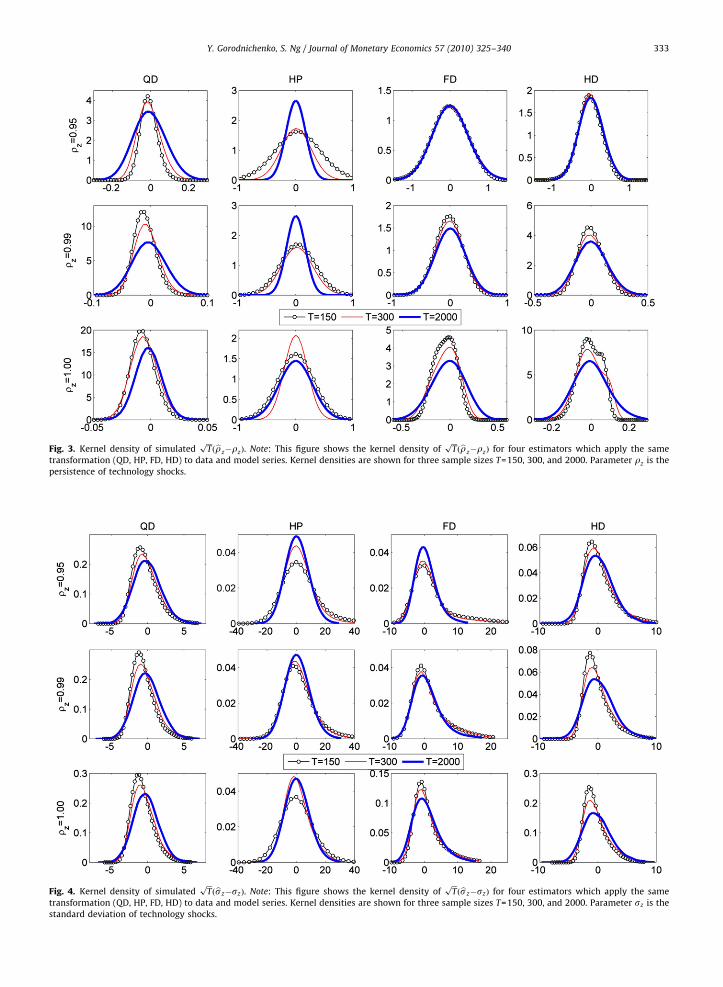
Fig. 3. Kernel density of simulated!!!T
p"brz#rz$. Note: This figure shows the kernel density of
!!!T
p"brz#rz$ for four estimators which apply the same
transformation (QD, HP, FD, HD) to data and model series. Kernel densities are shown for three sample sizes T=150, 300, and 2000. Parameter rz is thepersistence of technology shocks.
Fig. 4. Kernel density of simulated!!!T
p"bsz#sz$. Note: This figure shows the kernel density of
!!!T
p"bsz#sz$ for four estimators which apply the same
transformation (QD, HP, FD, HD) to data and model series. Kernel densities are shown for three sample sizes T=150, 300, and 2000. Parameter sz is thestandard deviation of technology shocks.
Y. Gorodnichenko, S. Ng / Journal of Monetary Economics 57 (2010) 325–340 333

Figs. 2–4 present the kernel density of the normalized estimator (i.e.!!!T
p" bY#Y$) for sample sizes of T=150 and 300.
Results are also reported for T=2000 to study the asymptotic properties of the estimators. Approximate normality of brz
when rz is close to one, is totally unexpected, given that the literature on integrated regressors prepared us to expect superconsistent estimators with Dickey–Fuller type distributions that are skewed. Instead, all densities are bell-shaped andsymmetric for all rzr1 with no apparent discontinuity as we increase rz to one. The normal approximation is not perfectin small samples, suggesting that some size distortion will occur if one uses the t statistic for inference. In unreportedresults, t-statistics constructed using Newey–West standard errors have rejection rates greater than the nominal size for allestimators except the HP, which can be undersized. For example, the rejection rate of the QD estimator for the two-sided t-test of rz at the true value of 1 is 0.055 when T=200 while for testing a at the true value of 0.33, the rejection rate is 0.21.This is larger than the nominal size of 0.05. As the sample size increases, the actual size gets closer (and eventuallyconverges) to the nominal rates. For example, at T=1000 for QD, the two-sided t-test of rz ! 1 has a rejection rate of 0.05,while the t test for a! 0:33 is 0.10. The QD and HD generally have better size than the FD and the HP. The finite sample sizedistortion seems to be a general problem with covariance structure estimators and not specific to the consideredestimators. Burnside and Eichenbaum (1996) reported similar results in covariance structure estimation with manyoveridentifying restrictions, also using the Newey–West estimator of the variance of moments.
5.1. Variations to the baseline model
In response to the finding in Cogley and Nason (1995b) that the basic real business cycle model has weak internalpropagation, researchers often augment the basic model to strengthen the propagation and to better fit the data at
ARTICLE IN PRESS
Table 3Augmented versions of the neoclassical growth model.
rz Data filter QD HD FD HP LT FD1 HP HPModel filer QD HD FD HP LT FD1 LT zt
(1) (2) (3) (4) (5) (6) (7) (8)
Panel A: serially correlated growth rate in technologyEstimate of k! 0
0.95 Mean #0.010 #0.001 0.001 #0.019 #0.180 #0.100 #0.224 #0.369St.dev. 0.063 0.058 0.050 0.160 0.165 0.035 0.038 0.106
0.99 Mean #0.014 #0.003 0.002 #0.016 #0.498 #0.021 #0.255 #0.429St.dev. 0.044 0.046 0.041 0.155 0.088 0.030 0.038 0.070
1.00 Mean #0.014 #0.003 0.003 #0.020 #0.600 #0.002 #0.256 #0.446St.dev. 0.038 0.039 0.035 0.161 0.029 0.028 0.038 0.058
Panel B: habit formation in consumptionEstimate of f! 0
0.95 Mean 0.020 0.008 0.006 #0.014 #0.410 #0.086 0.193 0.679St.dev. 0.075 0.073 0.071 0.255 0.339 0.066 0.382 0.074
0.99 Mean 0.019 0.009 0.008 0.023 #0.647 #0.018 0.495 0.637St.dev. 0.070 0.074 0.069 0.168 0.241 0.083 0.400 0.070
1.00 Mean 0.018 0.023 0.011 0.025 #0.702 0.011 0.603 0.622St.dev. 0.067 0.087 0.076 0.156 0.174 0.095 0.373 0.068
Panel C: preference shocks qtEstimate of a! 0:33
sq ! 0:50.95 Mean 0.344 0.335 0.361 0.329 0.465 0.299 0.591 0.337
St.dev. 0.040 0.025 0.080 0.075 0.126 0.043 0.037 0.1371.00 Mean 0.353 0.342 0.352 0.335 0.508 0.352 0.665 0.485
St.dev. 0.052 0.034 0.067 0.072 0.357 0.063 0.050 0.265sq ! 1:0
0.95 Mean 0.339 0.341 0.349 0.331 0.431 0.316 0.504 0.344St.dev. 0.023 0.030 0.049 0.060 0.103 0.022 0.031 0.022
1.00 Mean 0.347 0.347 0.357 0.340 0.611 0.341 0.529 0.364St.dev. 0.028 0.034 0.050 0.055 0.257 0.025 0.036 0.023sq ! 1:5
0.95 Mean 0.338 0.343 0.349 0.333 0.399 0.326 0.469 0.378St.dev. 0.021 0.030 0.042 0.053 0.078 0.017 0.020 0.024
1.00 Mean 0.341 0.346 0.353 0.338 0.515 0.338 0.477 0.391St.dev. 0.020 0.029 0.038 0.049 0.203 0.017 0.021 0.023
Note: Panels A and B: rz and k or f are estimated; a! 0:33 and sz ! 1 are fixed. Panel C: five parameters are estimated "a;rz;rq;sz ;sq$. The number ofsimulations is 2000. Sample size is T=200. LT is linear detrending, HP is Hodrick–Prescott filter, FD is first differencing, FD1 is first differencing with therestriction that rz ! 1, QD is quasi-differencing, HD is hybrid differencing, zt is detrending by the level of technology.
Y. Gorodnichenko, S. Ng / Journal of Monetary Economics 57 (2010) 325–340334

business cycle frequencies. One consideration is to introduce serial correlation in the growth rate of shocks to technologyby assuming ut ! "rz%k$ut#1#krzut#2%ezt . This specification generates serial correlation of k in the growth rate oftechnology when rz ( 1. The baseline model corresponds to k! 0. When data are simulated with k! 0 and k is estimatedfreely, the QD, HD, FD, and HP correctly find that k! 0 (Table 3, Panel A).
Habit in consumption is another popular way to introduce greater persistence in business cycle models. Consider theutility function: ln"Ct#fCt#1$#yLt where f measures the degree of habit in consumption. Data are generated with f set tozero. When f is freely estimated along with other parameters, the robust estimators again find bf to be numerically smalland not statistically different from zero for all values of rz (Table 3, Panel B).
A third variation to the baseline model is a preference shock Qt such that the utility is lnCt#yLt=Qt whereqt ! lnQt ! rqqt#1%eqt and eqt ) iid"0;s2
q$. In the simulations, rq ! 0:8 (so that the preference shock is stationary) andsq ! "0:5;1:0;1:5$. To conserve space, Panel C in Table 3 reports only estimates for a. Consistent with the results thus far, theHP estimates have the largest variability although the difference with other estimators is not as large as it was in the baselinemodel. Note that as sq increases, the difference across methods shrinks while the precision for all estimators improves.
A recurrent result is that the HP estimates have the largest variability and is computationally most intensive. Burnside(1998) reports that the HP filter removes variation potentially informative about the structural parameters but that the HPfiltered model and data series still have sufficient variability to discriminate competing theories of business cycles. Onepossibility for the results reported here is that the HP filters out more low frequency variation than other filters, and theparameters f and k are identified from these frequencies. Another possibility is that the HP implicitly uses many moreestimated autocovariances (recall that the inverse Fourier transform is applied to many autocovariances). This extensiveuse of sample autocovariances can also introduce variability to the estimator.
6. Non-robust estimators and a model with multiple rigidities
This section reports results for the non-robust estimators to illustrate how treatment of trends can bring aboutmisleading conclusions about the propagating mechanism of shocks. In addition to the basic stochastic growth model, theestimators are also compared for a model with many more endogenous variables.
6.1. Alternative detrending procedures
Up to this point, the considered approaches apply the same transformation to the data and the model variables. Muchhas been written about the effects of filtering on business cycle facts. King and Rebelo (1993) and Canova (1998) showedthat the HP filtered data are qualitatively different from the raw data. Canova (1998) showed that the stylized facts ofbusiness cycles are sensitive to the filter used to remove the trending components. Gregory and Smith (1996) used acalibrated business cycle model to investigate what type of trend can produce a cyclical component in the data that issimilar to the cyclical component in the model. Although these authors did not estimate a DSGE model on filtered data,they hinted that the parameter estimates can be adversely affected by filtering.
To investigate the consequences of using different and/or inappropriate filters, four combinations are considered:(A) the autocovariances are computed for linearly detrended model and data series; (B) the autocovariances are computedfor the first differenced model and data series with imposed rz ! 1; (C) the sample autocovariances are computed for HPfiltered data but the model autocovariances are computed for the linearly detrended variables; (D) the sampleautocovariances are computed for HP filtered data while the model autocovariances are computed for series normalized bythe level of technology, i.e., mt#zt where zt is the level of technology.
Each combination has been used in the literature (see e.g. Table 1). (A) and (B) are aimed to show the effects of imposingincorrect assumptions about trends. (C) and (D) illustrate the consequences when different trends are applied to the modeland the data.6 The results for the basic stochastic growth model are reported in Table 2. For (A), which is reported incolumn (5), the parameter estimates are slightly biased when rz ! 0:95. As rz increases, the estimates are strongly biased.This shows that when rz is close to unity yet stationary, assuming trend stationarity still yields imprecise estimates. Atrz ! 1, the mean of brz is 0.694 (instead of 1), the mean of ba is approximately 0.905 (instead of 0.33), the mean of bsz is 19.8(instead of 1). The case of rzr1 is empirically relevant because macroeconomic data are highly persistent and wellapproximated by unit root processes. These results show that linear detrending of nearly integrated data in non-linearestimation can lead to biased estimates of the structural parameters, reminiscent of the univariate finding of Nelson andKang (1981) that projecting a series with a unit root on time trend can lead to spurious cycles.
Turning to (B) in column (6) of Table 2, the estimates are fairly precise when rz is indeed equal to one, but as rz departsfrom one, the estimates get increasingly biased. Hence imposing a stochastic trend when the data generating process istrend stationary can lead to seriously distorted estimates. Results for combination (C) are reported in column (7) of Table 2.
ARTICLE IN PRESS
6 As a general observation, the starting values are very important for non-robust methods as the optimization routines can get stuck in local optima.With the robust estimators, the converged estimates do not change as the optimization starts from values other than the true parameters, though thesearch for global minimum was often long.
Y. Gorodnichenko, S. Ng / Journal of Monetary Economics 57 (2010) 325–340 335

The estimates of rz are downward biased while ba and bsz are upward biased. Taken at face value, these estimates suggest asignificant role for capital as a mechanism for propagating shocks in the model.
Results for (D) are reported in column (8) of Table 2. Here, the estimates of a often hit the boundary of the permissibleparameter space while estimates of sz are close to zero. The reason is that when zt has a unit root, shocks to mt#zt aretransitory and consumption adjusts quickly to the permanent technology shock. But the HP filtered data are seriallycorrelated. Thus, the estimator is forced to produce parameter values that can generate strong serial correlation in themodel variables. Results for (C) and (D) are consistent with the findings of Cogley and Nason (1995a), King and Rebelo(1993) and Harvey and Jaeger (1993). These papers suggest that the HP filter changes not only the persistence of the seriesbut also the relative volatility and serial correlation of the series. This translates into biased estimates of all parametersbecause the estimator is forced to match the serial correlation of the filtered data.
Clearly, large estimated values of a will alert the researcher that the model is likely misspecified. Suppose theresearcher allows for serially correlated shocks in technology growth by estimating k freely. Panel A in Table 3 shows thatthe non-robust methods now yield estimates of a around 0.4–0.5, which seem more plausible than when k was assumedzero. However, these estimates are achieved by having bk strongly negative and statistically significant when the true valueof k is zero. Suppose now the researcher modifies the model by allowing for habits in consumption. Evidently, theestimated habit formation parameter f is sensitive to which non-robust estimator is used. In particular, (A) has a strongdownward bias, while (B) produces a negative bias in bf when rz departs from one. On the other hand, (C) and (D) have astrong upward bias. With either modification, the fit of the misspecified models improves relative to the correctly specifiedmodel. However, these modifications should not have been undertaken as they do not exist in the data generating process.These examples indicate how the treatment of trends can mislead the researcher to augment correctly specified modelswith spurious propagation mechanisms to match the moments of the data.
Results for the model with an additional labor supply shock are reported in Table 3, Panel C. The estimates continue tobe biased although the biases tend to be smaller than in the baseline model with a single persistent shock. In general, a
ARTICLE IN PRESS
Table 4Smets and Wouters (2007) model.
rz Data filter QD HD FD HP LT FD1 HP HPModel filer QD HD FD HP LT FD1 LT zt
(1) (2) (3) (4) (5) (6) (7) (8)
Estimate of persistence in technology shocks rz
0.95 Mean 0.965 0.967 0.962 0.945 0.864 1.000 #0.100 1.000St.dev. 0.038 0.037 0.044 0.137 0.142 0.157
0.99 Mean 0.986 0.984 0.986 0.967 0.836 1.000 #0.114 1.000St.dev. 0.027 0.027 0.028 0.123 0.227 0.090
1.00 Mean 0.990 0.989 0.993 0.971 0.744 1.000 #0.123 1.000St.dev. 0.027 0.026 0.025 0.123 0.305 0.075
Estimate of investment adjustment cost f! 5:480.95 Mean 5.057 5.381 5.227 5.066 3.932 4.700 4.447 9.818
St.dev. 2.236 2.548 2.306 3.354 1.917 2.487 0.265 0.6090.99 Mean 5.432 5.563 5.373 5.095 5.595 5.236 4.366 9.662
St.dev. 2.321 2.463 2.404 3.012 2.647 2.794 0.257 0.5881.00 Mean 5.863 6.253 6.014 5.617 6.173 6.049 4.377 9.541
St.dev. 2.375 2.775 2.781 3.279 2.983 3.046 0.230 0.548
Estimate of habit formation l! 0:710.95 Mean 0.725 0.730 0.749 0.753 0.730 0.864 3.932 0.673
St.dev. 0.057 0.063 0.062 0.049 0.063 0.142 1.917 0.1340.99 Mean 0.699 0.718 0.719 0.718 0.543 0.744 0.908 0.941
St.dev. 0.056 0.053 0.062 0.134 0.177 0.053 0.033 0.0061.00 Mean 0.686 0.711 0.716 0.709 0.470 0.731 0.912 0.940
St.dev. 0.056 0.055 0.064 0.145 0.261 0.057 0.028 0.005
Estimate of wage adjustment probability xw ! 0:730.95 Mean 0.704 0.730 0.734 0.686 0.657 0.759 0.484 0.220
St.dev. 0.073 0.063 0.075 0.117 0.105 0.077 0.085 0.0190.99 Mean 0.686 0.704 0.709 0.659 0.530 0.718 0.458 0.213
St.dev. 0.081 0.065 0.079 0.125 0.214 0.084 0.078 0.0161.00 Mean 0.673 0.697 0.700 0.641 0.457 0.700 0.444 0.210
St.dev. 0.092 0.068 0.083 0.138 0.262 0.091 0.072 0.015
Note: The number of simulations is 2000. Sample size is T=150. LT is linear detrending, HP is Hodrick–Prescott filter, FD is first differencing, FD1 is firstdifferencing with the restriction that rz ! 1, QD is quasi-differencing, HD is hybrid differencing, zt is detrending by the level of technology.
Y. Gorodnichenko, S. Ng / Journal of Monetary Economics 57 (2010) 325–340336

smaller rz and a larger sq lead to smaller biases. In some cases, one finds bsq4 bsz, so that the researcher may be tempted toconclude that preference shocks have larger volatility than shocks to technology while the opposite is true.
6.2. The Smets and Wouters model
Although the baseline model is an illuminating laboratory to evaluate how the estimators perform, it is overlysimplistic. To assess the properties of the estimators in a more realistic setting, consider the model of Smets andWouters (2007) (henceforth SW). Treating SW’s estimates for the post-1982 sample as the true parameter values, series ofsize T=150 are generated and the estimators are applied to the generated series. To separate identification issues fromissues related to the treatment of trends, only four parameters are estimated: persistence of technology shocks rz whosetrue value varies across simulations; investment adjustment cost f whose true value is 5.48; external habit formation inconsumption l whose true value is 0.71; and Calvo’s probability of wage adjustment xw whose true value is 0.73.
The results are reported in Table 4. All robust methods yield precise estimates of the parameters. Although the HPcontinues to be less precise, the difference with the other three robust estimators is smaller than in the baseline model. Asimilar feature was observed when the two-shock and one-shock neoclassical growth models were compared. Thesedifferences between the baseline and the more complicated models can occur for several reasons. First, in larger modelswith many other structural shocks, technology shock explains only a fraction of variation in key macroeconomic variables.The HP estimator may simply need more shocks to identify the parameters. Second, bigger models impose manymore cross equation restrictions that may improve the efficiency of some estimators more than others. The generalobservation, however, is that the proposed robust estimators perform reasonably well for all values of rz in simple andmore complex models.
In contrast, the non-robust estimators (A) through (D) have dramatic biases in all four parameters being estimatedwhen (i) the filter used for the model and the data are different, when (ii) the assumed trends are different from trends inthe data generating process, or when (iii) the data are stationary but highly persistent. Obviously, the impulse responses(and other analyses related to the role of rigidities in amplification and propagation of shocks in business cycle models)based on these biased estimates of the structural parameters will be misleading. As an illustration, Fig. 5 highlights thedifference between the true response of key macroeconomic variables to a technology shock in the SW model and theresponses based on parameter estimates from approaches (A) through (D). For instance, consider the response of
ARTICLE IN PRESS
0 5 10 15 200
0.5
1
1.5
2 Output
0 5 10 15 20!0.5
0
0.5
1
1.5
2 Consumption
0 5 10 15 20!1
0
1
2
3 Investment
0 5 10 15 20!0.5
0
0.5
1
1.5 Wages
0 5 10 15 20!1
!0.5
0
0.5 Employment
0 5 10 15 20!0.15
!0.1
!0.05
0
0.05 Inflation
True (LT,LT) (FD1,FD1) (HP,LT) (HP,zt)
Fig. 5. Estimated impulse responses functions to a technology shock in Smets and Wouters (2007) model. Note: This figure plots impulse responsefunctions based on parameter estimates obtained from estimators applying different filters to model and data series when the data are generated by theSmets and Wouters (2007) model. LT is projection on a linear time trend. FD1 is first differencing. HP is the Hodrick–Prescott filter. The shock is a 1percent increase in the level of technology. Persistence of technology shock is rz ! 0:99. See supplemental material for other impulse responses.
Y. Gorodnichenko, S. Ng / Journal of Monetary Economics 57 (2010) 325–340 337

consumption. Estimates from approaches (A) and (C) imply grossly understated responses. Estimates from approach (D)suggest a considerably more delayed consumption response than the true one. The consumption response implied byapproach (B) is qualitatively similar to the true response, but the responses are noticeably different quantitativelyespecially when rz is further away from one.
7. Extensions and implementation issues
This section discusses several practical issues and extensions pertaining to the robust estimators.
7.1. Multiple shocks
The reduced form solution (1) can be easily generalized to other models and takes the form
bmt !P bmt#1%But
ut ! rut#1%Set "3$
where ut is now a vector of exogenous forcing variables, et is a vector of innovations in ut, and the matrices P, B, S, r are ofconformable sizes.
Suppose there are J univariate shock processes, each characterized by
"1#rjL$ujt ! ejt ; j! 1; . . . ; J
where some J* of the rj may be on the unit circle. Define
Dr"L$ !YJ&
j ! 1
"1#rjL$
Now the quasi-differencing operator is the product of the J* polynomials in lag operator. Once the model is solved to arriveat (3), one can compute moments for Dr"L$ bmt . Whether none, one, or more shocks are permanent, the autocovariances ofthe transformed variables are well defined. For example, if one knows that shocks to tastes dissipate quickly whiletechnology shocks zt are highly persistent, one can still use "1#rzL$ as D
r.
7.2. Likelihood estimation
As likelihood and Bayesian estimation is commonly used in the DSGE literature, one may wonder how the ideasconsidered in this paper can be implemented in likelihood based estimation. Suppose one can write the model in a statespace form which involves using the measurement equations to establish a strict correspondence between the detrendedseries in the model and in the data. Then one can derive the likelihood which makes maximum likelihood (MLE) andBayesian estimation possible.
As an example, consider the model given in (3). The measurement equation corresponding to the FD estimator is
xt !Hst ! *C #C 0+st "4$
where xt is the vector of filtered variable, C is the selection matrix, and s0t ! " bmt ; bmt#1;ut$ is the state vector. Thecorresponding transition equation is
bmt
bmt#1
ut
2
64
3
75!
P 0 BrI 0 0
0 0 r
2
64
3
75
bmt#1
bmt#2
ut#1
2
64
3
75%BS
0
S
2
64
3
75et
or
st !P&st#1%B&et "5$
with et ) i:i:d:"0;S$. The measured variable xt is stationary irrespective of whether bmt has stochastic or deterministictrends. For the QD0 estimator, H! *C #rC 0+. As with all quasi-differencing estimators, the treatment of initial conditionis important especially when there is strong persistence. In simulations with the first observation held fixed, the MLEversion of the FD gives precise estimates, but the t statistics are less well approximated by the normal distributioncompared to MM-FD (see supplementary material).
For the other three estimators, the extension to MLE is either not possible or not practical. For MLE-HP, one would needto write out the entire data density of the HP filtered data, and the Jacobian transformation from the unfiltered to filtereddata involves an infinite dimensional matrix. For the QD estimator, recall that the autocovariances are normalized by thevariance. By analogy, MLE-QD would require modifying the score vector. Although such modification is possible in theory,it is not straightforward to implement. For the HD estimator, the MLE implementation is cumbersome because HD exploits
ARTICLE IN PRESSY. Gorodnichenko, S. Ng / Journal of Monetary Economics 57 (2010) 325–340338

covariances of variables computed with different filters. The difference between the MM and MLE really boils down to achoice of moments, and the MM is more straightforward to implement.
7.3. Computation
Moments of the filtered model variables can be computed analytically or by using simulations. We use the analyticalmoments whenever possible since it tends to be much faster than simulations and it does not have simulation errors.Although there are a variety of methods for analytical calculations, a method that is especially attractive for large models isto combine the measurement equation xt=Hst and the state equation st !P&st#1%B&et to obtain
xtst
" #!
0 HP&
0 P&
" # xt#1
st#1
" #%
HB&
B&
" #et
Let w0t ! "x0t ; s
0t$ so that
wt !D0wt#1%D1et
The variance matrix Ow"0$ ! E"wtw0t$ can now be computed by iterating the equation
O"i$w "0$ !D0O"i#1$
w "0$D00%D1SD0
1 "6$
until convergence. The autocovariance matrices can then be computed as Ow"j$ !Dk0Ow"0$. Since one is only interested in
computing the moments of variables in the measurement vector xt , one can iterate Eq. (6) until the block that correspondsto xt converges, i.e. JO"i$
x "0$#O"i#1$x "0$Joe.
To compute the moments of the HP filtered data, observe that the HP filtered series can alternatively be obtainedas follows:
HP"L$dt !HP% "L$Ddt !l"1#L$"1#L#1$2
1%l"1#L$2"1#L#1$2Ddt
In practice, using HP+(L) and the autocovariances for Ddt and D bmt tends to give more stable results when rz is close to one.It is possible to speed up estimation based on HP filtered series by using a smaller number of leads and lags at the cost oflarger approximation errors.7
Finally, a note on the treatment of stationary variables is in order. Recall that in the stochastic growth model,m&
t ! "gt; gt;0$ when jrzjo1 and m&t ! "ut%gt;ut%gt;0$ when jrzj! 1, where the third component of m*
t is the trend forlabor supply, lt. Since lt has no deterministic or stochastic trend component, the autocovariances are computed for lt andnotblt , though the results do not change materially if the filtered series were used. In general, if the j-th component of m*
t iszero, it is understood that the autocovariances are computed for the level of the variable both in the model and in the data.An alternative is to deal with these non-trending variables through the measurement equation. Then some variables can bequasi-differenced or first-differenced, while others require no transformation.
8. Concluding remarks
A realistic situation encountered with estimation of DSGE model is that (a) the data are trending; (b) deviations fromthe trend are persistent; (c) the researcher does not know whether the data generating process is difference or trendstationary. This paper shows that the treatment of trends can significantly affect the parameter estimates of DSGE modelsand propose several robust approaches that produce precise estimates without the researcher having to take a stand oftrend specification. The key is to apply the same filter to the data and the model variables to yield well-defined momentsfor the estimation of the structural parameters. Several filters can be used in methods of moments estimation. Theseestimators have approximately normal finite sample distributions. Undoubtedly, the estimators require further scrutinyand can be improved in various dimensions.8 The present analysis is a first step in the sparse literature on non-linearestimation when the data are highly persistent.
Appendix A. Supplementary data
Supplementary data associated with this article can be found in the online version at doi:10.1016/j.jmoneco.2010.02.008.
ARTICLE IN PRESS
7 A simulation procedure can also be considered. For eachY, the model is used to generate j=1,y,R samples of size T and the moments are computed.Averaging over j gives om
HP . This procedure is computationally more intensive and the results are similar to the one considered here.8 For example, one can use the bootstrap developed for covariance structures in Horowitz (1998) to correct for small-sample biases. One might also
consider a model-based instead of a data-based weighting matrix computed. Finally, one may use simulation based estimators, see Coibion andGorodnichenko (2010) for an example.
Y. Gorodnichenko, S. Ng / Journal of Monetary Economics 57 (2010) 325–340 339

References
Abowd, J.M., Card, D., 1989. On the covariance structure of earnings and hours changes. Econometrica 57 (2), 411–445.Altig, D., Christiano, L., Eichenbaum, M., Linde, J., 2004. Firm-specific capital, nominal rigidities, and the business cycle, FRB Cleveland WP 2004-16.Altonji, J., Segal, L., 1996. Small-sample bias in GMM estimation of covariance structures. Journal of Business and Economic Statistics 14 (3), 353–366.Altug, S., 1989. Time-to-build and aggregate fluctuations: some new evidence. International Economic Review 30, 889–920.Anderson, G., Moore, G., 1985. A linear algebraic procedure for solving linear perfect foresight models. Economic Letters 17 (3), 247–252.Baxter, M., King, R., 1999. Measuring business cycles: approximate bandpass filters for economic time series. Review of Economics and Statistics 81 (4),
575–593.Blanchard, O., Kahn, C., 1980. The solution of linear difference models under rational expectations. Econometrica 48, 1305–1313.Bouakez, H., Cardia, E., Ruge-Murcia, F.J., 2005. Habit formation and the persistence of monetary shocks. Journal of Monetary Economics 52, 1073–1088.Burnside, C., 1998. Detrending and business cycle facts: a comment. Journal of Monetary Economics 41, 513–532.Burnside, C., Eichenbaum, M., 1996. Small-sample properties of GMM-based Wald tests. Journal of Business and Economic Statistics 14, 294–308.Burnside, C., Eichenbaum, M., Rebelo, S., 1993. Labor hoarding and the business cycle. Journal of Political Economy 101, 245–273.Canova, F., 1998. Detrending and business cycle facts. Journal of Monetary Economics 41, 475–512.Canova, F., 2008. Estimating DSGE models with unfiltered data. Mimeo.Canova, F., Ferroni, F., 2008. Multiple filtering devices for the estimation of cyclical DSGE models. Mimeo.Canova, F., Sala, L., 2009. Back to square one: identification issues in DSGE models. Journal of Monetary Economics 56, 431–449.Christiano, L., den Haan, W., 1996. Small-sample properties of GMM for business cycle analysis. Journal of Business and Economic Statistics 14, 309–327.Christiano, L., Eichenbaum, M., 1992. Current real-business-cycle theories and aggregate labor-market fluctuations. American Economic Review 82,
430–450.Christiano, L.J., Eichenbaum, M., Evans, C.L., 2005. Nominal rigidities and the dynamic effects of a shock to monetary policy. Journal of Political Economy
113 (1), 1–45.Clarida, R., Gali, J., Gertler, M., 2000. Monetary policy rules and macroeconomic stability: evidence and some theory. Quarterly Journal of Economics 115,
147–180.Cogley, T., 2001. Estimating and testing rational expectations models when the trend specification is uncertain. Journal of Economic Dynamics and
Control 25, 1485–1525.Cogley, T., Nason, J., 1995a. Effects of the Hodrick–Prescott filter on trend and difference stationary time series: implications for business cycle research.
Journal of Economic Dynamics and Control 19, 253–278.Cogley, T., Nason, J., 1995b. Output dynamics in real business cycle models. American Economic Review 85, 492–511.Coibion, O., Gorodnichenko, Y., 2010. Strategic interaction among heterogeneous price-setters in an estimated DSGE model. Review of Economics and
Statistics, forthcoming.Del Negro, M., Schorfheide, F., Smets, F., Wouters, R., 2007. On the fit of new Keynesian models. Journal of Business and Economic Statistics 25, 123–143.Dib, A., 2003. An estimated Canadian DSGE model with nominal and real rigidities. Canadian Journal of Economics 36, 949–972.Doorn, D., 2006. Consequences of Hodrick–Prescott filtering for parameter estimation in a structural model of inventory. Applied Economics 38,
1863–1875.Faia, E., 2007. Finance and international business cycles. Journal of Monetary Economics 54, 1018–1034.Fernandez-Villaverde, J., Rubio-Ramirez, J.F., 2007. Estimating macroeconomic models: a likelihood approach. Review of Economic Studies 74 (4),
1059–1087.Fuhrer, J., 1997. The (un)importance of forward-looking behavior in price specifications. Journal of Money, Credit, and Banking 29, 338–350.Fuhrer, J., Rudebusch, G., 2004. Estimating the Euler equation for output. Journal of Monetary Economics 51, 1133–1153.Fukac, M., Pagan, A., 2006. Limited information estimation and evaluation of DSGE models, NCER Working Paper No. 6.Gorodnichenko, Y., Mikusheva, A., Ng, S., 2009. A simple root-t consistent and asymptotically normal estimator for the largest autoregressive root. Mimeo.Gregory, A., Smith, G., 1996. Measuring business cycles with business-cycle models. Journal of Economic Dynamics and Control 20, 1007–1025.Harvey, A., Jaeger, A., 1993. Detrending, stylized factors, and the business cycle. Journal of Applied Econometrics 8, 231–247.Horowitz, J., 1998. Bootstrap methods for covariance structures. Journal of Human Resources 33, 39–61.Ireland, P., 1997. A small structural quarterly model for monetary policy evaluation. Carnegie-Rochester Conference Series on Public Policy 47, 83–108.Ireland, P., 2001. Sticky-price models of the business cycle: specification and stability. Journal of Monetary Economics 47, 3–18.Ireland, P., 2004. Technology shocks in the new Keynesian model. Review of Economics and Statistics 86, 923–936.Iskrev, N., 2010. Local identication in DSGE models. Journal of Monetary Economicss 57 (2), 189–202.Kim, J., 2000. Constructing and estimating a realistic optimizing model of monetary policy. Journal of Monetary Economics 45, 329–359.King, R., Rebelo, S., 1993. Low frequency filtering and real business cycles. Journal of Economic Dynamics and Control 17, 207–231.Komunjer, I., Ng, S., 2009. Dynamic identification of DSGE models. Unpublished manuscript, Columbia University.Kydland, F., Prescott, E., 1982. Time to build and aggregate fluctuations. Econometrica 50, 1345–1370.Lubik, T., Schorfheide, F., 2004. Testing for indeterminacy: an application to U.S. monetary policy. American Economic Review 94, 190–217.McGrattan, E., Rogerson, R., Wright, R., 1997. An equilibrium model of the business cycle with household production and fiscal policy. International
Economic Review 38, 267–290.Nelson, C., Kang, H., 1981. Spurious periodicity in inappropriately detrended time series. Econometrica 49, 741–751.Newey, W., McFadden, D., 1994. Large sample estimators and hypothesis testing. In: Engle, R., Intriligator, D. (Eds.), Handbook of Econometrics, vol. 4.
North Holland, Amsterdam (Chapter 36).Ruge-Murcia, F., 2007. Methods to estimate dynamic stochastic general equilibrium models. Journal of Economic Dynamics and Control 31, 2599–2636.Sbordone, A., 2006. U.S. wage and price dynamics: a limited-information approach. International Journal of Central Banking 2 (3), 155–191.Sims, C., 2002. Solving linear rational expectations models. Computational Economics 1/2, 1–20.Singleton, K.J., 1988. Econometric issues in the analysis of equilibrium business cycle models. Journal of Monetary Economics 21, 361–368.Smets, F., Wouters, R., 2003. An estimated dynamic stochastic general equilibrium model of the euro area. Journal of the European Economics Association
1 (5), 1123–1175.Smets, F., Wouters, R., 2007. Shocks and frictions in US business cycles: a Bayesian DSGE approach. American Economic Review 97, 586–606.
ARTICLE IN PRESSY. Gorodnichenko, S. Ng / Journal of Monetary Economics 57 (2010) 325–340340