journal of mechanical engineering vol 17(1), 135-156, 2020

Journal of Mechanical Engineering Vol 17(1), 135-156, 2020

___________________

ISSN 1823-5514, eISSN2550-164X Received for review: 2019-07-13 © 2020 Faculty of Mechanical Engineering, Accepted for publication:2020-03-20

Universiti Teknologi MARA (UiTM), Malaysia. Published:2020-04-01

Fatigue Life Assessment Approaches Comparison Based on

Typical Welded Joint of Chassis Frame

Maksym Starykov*

Liebherr Container Cranes Ltd, Ireland

[email protected]

ABSTRACT

There are many approaches to the durability calculation that are used in

engineering practice. At the same time the existing accident studies show that

the leading position is still hold by fatigue failures. This means that there is

still no universal approach to fatigue problem solution, and the existing

approaches have their limitations. In addition, there is lack of information

about the comparison between the precision of the obtained results using

different approaches. In this paper different fatigue life calculation methods,

like nominal stress, hot spot stress, notch stress and fracture mechanics are

used to calculate the durability of T-type welded joint. The obtained results

are compared with the fatigue test ones and the approaches, which give the

closest results, are found.

Keywords: Metal Fatigue; Nominal Stress; Hot Spot Stress; Notch Stress;

Fracture Mechanics

Introduction

Time varying working loads are typical for metal constructions of chassis

frames, material handling machines, ship hulls etc. According to accident

studies for offshore structures [1], that took place in the North Sea, for period

from 1972 to 1992, all reasons have been split into several groups according

to their significance:

• fatigue 25%;

• structure collision with a ship 24%;

• dropping objects 9%;

Maksym Starykov

136

• corrosion 6%

In spite of the existence of different guides and approaches that have

being used for fatigue design the significant part of failures caused by fatigue

reveals the imperfection of using analysis methods. That is why the

development of a new methodology is the pressing issue.

Modern fatigue design approaches are based on stress information

about designing joint received from the finite element analysis of a structure.

This gives the possibility of using the local stress in the probable area of the

fatigue crack appearance instead of using nominal stress in the joint and

broadens horizons for further enhancements.

Metal fatigue phenomena have been attracting a lot of

researchers‘interest for a long time and with the welding invention this

interest even increased. The main problem was that all of researches solved

particular problems (i.e. the effect of mean stress on the durability etc.) but

there was no general practical approach with thorough step by step

recommendations for the practicing engineers how to perform the analysis.

The situation is changed during last decade when International Institute of

Welding [2]-[5], British Standard [6][7], and DNV [8][9] have represented

researches that are summarized in particular guides for the fatigue analysis

with detailed description of practical utilization of the approaches, starting

from mesh description and finishing with recommendations about what type

of S-N curve to use.

With the aforementioned guides in the place the question of the

analysis result validation has appeared. Thus, many researches have their

goal to compare the fatigue experiment and analysis results [10]-[13]. The

main problem in our opinion is that in those researches only one method of

the analysis is compared with the test results. But at the same time in

engineering practice at least four of them are frequently used:

• nominal stress approach;

• hot spot stress approach;

• notch stress approach;

• fracture mechanics approach.

In this paper the comparison between main analytical approaches and

test results for the fatigue life assessment has been done. This comparison

could help to the practicing engineer to decide which approach to the

durability analysis is more accurate for designing of similar joints.

For the analysis the T-type welded joint (Figure 1) is chosen. Despite

the fact that this type of connection is typical for a chassis frame, it is not

covered in the researches. All the existing analysis, done for the T weld

connection [10]-[13], have their welded gusset plate serving for stress

concentration purpose only, when in the T-weld connection that is studied,

the force and moment are transmitted to the main plate (crossbeam) through

the gusset plate (longeron).

Fatigue Life Assessment Approaches Comparison

137

In the following chapters, the durability of the joint is obtained using

testing and different analysis approaches. The results are discussed in clause

“Discussion of the obtained results”.

Fatigue test results The article objective is to define the approaches that give the closest result of

fatigue life assessment to ones taken from fatigue test for T-type welded joint

of a chassis frame [14].

Figure 1: Crossbeam to longeron T-type welded joint from 93571 ODAZ

trailer chassis frame (1 – crossbeam; 2 – longeron) acc. [14]

Specimens have been tested using symmetric stress cycle (R = -1).

The crossbeam was fixed using 4 holes of 10 mm in diameter and the 2

forces were applied using the 2 holes of 14 mm in diameter in longeron. The

fact of the crossbeam vertical deformation amplitude increasing beyond 30%

has been used as a collapse criterion to stop the fatigue tests. The six joints

have been tested on 6 different stress levels (Table 1). The fatigue curve of

Weibull type has been used:

𝑚𝑤 ∙ lg(𝜎) + 𝑙𝑔𝑁 = 𝐶𝑤 (1)

where is the nominal stress, MPa; N – durability, cycles; mw and Cw are

empirical parameters. Using linear interpolation on test data (Figure 2), the

following values of parameters in Equation (1) have been found: mw = -

2.489; Cw = 3.3319.

Table 1: Fatigue test results for T-weld joint crossbeam to longeron acc. [14]

Max. nominal stress

in the crossbeam

(amplitude)

, MPa

160 140 120 100 80 60

Fatigue life N,

cycles 39800 63100 102300 182000 478600 2089300

Maksym Starykov

138

Based on Equation (1), the fatigue life for stress amplitude 𝜎𝑎_𝑛𝑜𝑚 =81.5 MPa with 50% failure probability is 425 100 cycles.

Figure 2: Nominal stress in crossbeam vs the number of stress cycles (S-N

curve) obtained from fatigue tests acc. [14]

Fatigue life with failure probability of 2.3% has been calculated using

next Equation (2):

𝑙𝑔𝑁𝑃=2.3% = 𝑙𝑔𝑁𝑃=50% − 𝑧𝑃=2.3% ∙ 𝑙𝑔𝜎𝑁 = 187 280 (2)

where d – standard deviation amount below mean value; zP=2.3%= zP=97.7%=2

(quantile for failure probability of 2.3%); 𝑙𝑔𝜎𝑁 - standard deviation of 𝑙𝑔𝑁,

0.178, p. 20 [2] for the specimen amount n<10.

Figure 3: Test machine acc. [14]

https://www.multitran.ru/c/m.exe?t=258051_1_2&s1=%EA%E2%E0%ED%F2%E8%EB%FC


139

Fatigue life with failure probability of 97.7% has been calculated

using Equation (3):

𝑙𝑔𝑁𝑃=97.7% = 𝑙𝑔𝑁𝑃=50% + 𝑧𝑃=97.7% ∙ 𝑙𝑔𝜎𝑁 = 964 920 (3)

Traditionally beam theory for nominal stress calculation is used for S-

N curve. But that stress is not representative for current joint because the

fracture happens not in the crossbeam outer layers but in the area of welding

seam transition to the longeron (Areas 1 and 2, Figure 1).

P1 = 5519 N; P2 = 6319 N

(a) (c)

beam finite elements boundary

conditions

shell finite elements boundary

conditions

(b) (d)

Figure 4: Crossbeam stress calculation using finite elements of beam and

shell types

Using the shell finite elements gives realistic results. Maximum stress

in crossbeam for the beam finite element (Figure 4(a) and (b)) is 81.5 MPa,

and for shell finite element (Figure 4(c) and (d)) is 159 MPa. Moreover,

stress state of crossbeam in the area of welding seam is not more uniaxial one

but complex i.e. all three principal stresses have non zero magnitudes.

Nominal Stress approach The first step of nominal stress analysis [6] is to find among the variety of

joint types with boundary conditions (showed in standard) the one that

corresponds to the designing joint. But for currently calculating T-type

welded connection the similar joint type does not exist. For the first look

Maksym Starykov

140

Type 5.3 (class F2, Figure 5(a)), clause 2, Table 1 [6], could be taken, but its

boundary conditions are different from analysing connection: unlike to the

join from the standard the gusset plate (longeron) does not takes any load.

That is why it cannot be used further on. The joint on Figure 5(b) cannot be

used for calculating either, because its boundary conditions differ from

designing joint’s ones. It is also not clear stress in which element is taken for

nominal (loading scheme is not shown).

Figure 5: Nominal Stress approach joint classification

Hot spot stress approach This approach [3] allows calculating the joint fatigue life using its stress-

strain state data obtained from the finite element analysis. The following joint

modelling techniques are suggested to be used:

• Modelling using shell finite elements. In this case welding seam is to

be create in such ways:

o Model without welding seams;

o Using oblique shell elements to model welding seams;

o Using shell element with increased thickness for welding

seams modelling;

• Solid modelling with volume finite elements. Idealized welding seam

shape is used.

Modelling using shell elements Model without welding seams According to IIW Recommendations [3] welded element durability is to be

calculated based on stress that acts in the weld toe. However, because of

using linear elastic metal behaviour and the fact that the real weld profile is

unknown on design stage, there is no possibility to use directly the stress read

from welding toe. Instead, it has been proposed to use stress extrapolated

value based on stress in the welding seam vicinity, so called Structural Stress.


141

For our case (model consists of 4 node linear shell finite elements with edge

of 1.6 mm near the stress concentration point) the hot spot stress is given by:

𝜎ℎ𝑠 = 1.67 ∙ 𝜎0.4𝑡 − 0.67 ∙ 𝜎1𝑡 (4)

where σ0.4·t - stress value at the distance of 0.4·t from the weld toe (the first

extrapolation point); σ1·t - stress value at the distance of 1·t from the weld toe

(the second extrapolation point); t – longeron thickness, 4 mm.

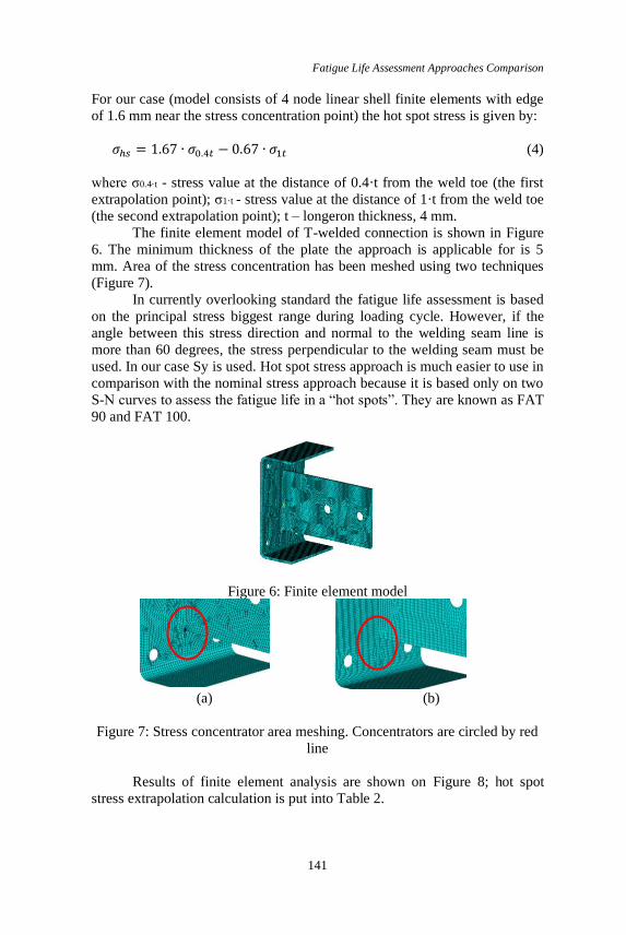
The finite element model of T-welded connection is shown in Figure

6. The minimum thickness of the plate the approach is applicable for is 5

mm. Area of the stress concentration has been meshed using two techniques

(Figure 7).

In currently overlooking standard the fatigue life assessment is based

on the principal stress biggest range during loading cycle. However, if the

angle between this stress direction and normal to the welding seam line is

more than 60 degrees, the stress perpendicular to the welding seam must be

used. In our case Sy is used. Hot spot stress approach is much easier to use in

comparison with the nominal stress approach because it is based only on two

S-N curves to assess the fatigue life in a “hot spots”. They are known as FAT

90 and FAT 100.

Figure 6: Finite element model

(a) (b)

Figure 7: Stress concentrator area meshing. Concentrators are circled by red

line

Results of finite element analysis are shown on Figure 8; hot spot

stress extrapolation calculation is put into Table 2.

Maksym Starykov

142

(a) M + (b) M-

Figure 8: Sy stress graphical plots for the boundary conditions shown in

Figure 4 (mesh is acc. Figure 7 (a))

Table 2: “Hot spot” stress approximation and durability assessment

Fin

ite

elem

ent

mes

h t

ype

in t

he

conce

ntr

ator

vic

init

y

Hot spot stress

calculated based on

Sy, MPa

“hot

spot”

str

ess,

σhs_

max

(+M

),

MP

a

“hot

spot”

str

ess,

σhs_

max

(-M

),

MP

a

“hot

spot”

str

ess

range,

Δσ

hs

acc.

(4),

MP

a

Thic

knes

s co

rrec

tion

1 Fatigue life

nea

rest

to t

he

wel

din

g s

eam

poin

t,

𝜎0

.4∙𝑡

fart

hes

t fr

om

the

wel

din

g s

eam

poin

t,

𝜎0

1.0

∙𝑡

Fai

lure

pro

bab

ilit

y

2.3

%

Fai

lure

pro

bab

ilit

y

50%

*

Fai

lure

pro

bab

ilit

y

97.7

%2 *

Figure

7(а) 497 355 592 -592 1184

Yes 1 205 2 735 6 209

No 6 239 14 161 32 140

Figure 7(b)

439 281 545 -545 1090 Yes 1 544 3 508 7 962

No 7 996 18 150 41 200

*Durability corresponding to different failure probabilities than other than 2.3% are

calculated acc. (2) and (3).

The numbers that come after letters “FAT” indicate stress level in

MPa that corresponds to 2·106 cycle durability. The general equation for

these S-N curves is as follows:

1 Thickness correction according to [3] could be calculated for as-welded T-joints as 𝑓(𝑡) =

(𝑡𝑟𝑒𝑓

𝑡𝑒𝑓𝑓)

0.2

= 1.73, where 𝑡𝑟𝑒𝑓 = 25𝑚𝑚, 𝑡𝑒𝑓𝑓 = 4𝑚𝑚 is the joint plate thickness. This factor is

used for FAT scaling, so for FAT 100 it will be FAT 173. This correction is used normally for plates thicker than 25 mm, but the guide says that „in the same way a benign effect might be

considered, but this should be verified by component test“.

2Durability corresponding to different failure probabilities are calculated acc. (2) and (3).


143

∆𝜎ℎ𝑠𝑚 ∙ 𝑁 = 𝐶 (5)

where Δσhs = σhs_max - σhs_min - stress range in the «hot spot», σhs_max -

maximum hot spot stress of a cycle, σhs_min - minimum hot spot stress of a

cycle; m – index of power, 3.0; С – coefficient, 2·1012; N – life cycle.

Plane model with shell finite elements. Welding seam is modelled by

oblique shell elements

The main concept of welding seam modelling is shown in Figure 9 and

meshed model – in Figure 10 (a).

Figure 9: Welding seam modelling with oblique shell elements

For this case first principal stress is perpendicular to the welding

seam. That is why it is used for the further analysis.

(a) Finite element model (b) First principal stress graphical plot

Figure 10: Example of welding seam modelling with oblique shell elements.


1

11

X

Y

Z

2 mm crack

FEB 5 2019

18:48:41

ELEMENTS

SEC NUM

Maksym Starykov

144

Hot spot stress calculated based on S1,

MPa

“hot

spot”

str

ess

range,

Δσ

hs

acc.

(4),

MP

a

Thic

knes

s co

rrec

tion†

Fatigue life nea

rest

to t

he

wel

din

g

seam

poin

t, 𝜎

0.4

∙𝑡

fart

hes

t fr

om

the

wel

din

g s

eam

poin

t,

𝜎 1.0

∙𝑡

Fai

lure

pro

bab

ilit

y

2.3

%

Fai

lure

pro

bab

ilit

y 5

0

% *

Fai

lure

pro

bab

ilit

y

97.7

% *

274 194 328 Yes 56 680 128 500 291 700

No 293 500 666 100 1 512 000



Solid model with volume finite elements Solid model of the crossbeam-longeron welding connection is shown in

Figure 11. To reduce the computation time during model stress analysis only

one half of the model has been created. 20 node Solid finite element with

decreased integration and edge size of 4 mm is used.

The distances from the weld toe to the extrapolation points are the

same (0.4·t to the first (nearest to weld) extrapolation point and 1·t to the

second extrapolation point). Stress analyses result is shown in Figure 12.

Figure 11: Crossbeam-

longeron welding connection

solid model.

Figure 12: 1st principal stress graphical.

Plots/ for the boundary conditions shown in

Figure 4



145

Hot spot stress calculated based

on S1, MPa

“hot

spot”

str

ess

range,

Δσ

hs a

cc.

(4),

MP

a

Fatigue life

nearest to the

welding seam

point, 𝜎0.4∙𝑡

farthest from the welding

seam point,

𝜎1,0∙𝑡

Failure probability

2.3%

Failure probability

50% *

Failure probability

97.7% *

335 228 407 29 670 67 300 152 800



Notch Stress approach This approach [4, 5] demands solid model creation and volume finite element

mesh using. For the plate thickness less than 5 mm, the notch radius of 0.05

mm instead of 1 mm has to be used, special attention must be paid to a weld

seam modelling particularly in the area where welding seam material merges

to the main metal (Figure 13 b) because the stress in this area is used for the

fatigue life estimation. Only one S-N curve uses for this analysis (FAT 630)

which equation takes a form of:

∆𝜎𝑚 ∙ 𝑁 = 𝐶 (6)

where the equation parameters are m = 3; 𝐶 = (𝐹𝐴𝑇)𝑚 ∙ 2 ∙ 106. In addition

to the weld toe modelling radius (Figure 14) the approach specifies the

welding seam geometry creation method, finite element size etc.

(a) (b)

Figure 13: Crossbeam-longeron welding connection model for notch stress

analysis

1

X

Y

Z

MAR 25 2019

09:49:11

ELEMENTS

1

MAR 25 2019

09:49:33

ELEMENTS

Maksym Starykov

146

Figure 14: Welding seam modelling requirements

Due to the high level of detail needed for welding area modelling, the

scope of problem increases with the growth of the joint complexity. That is

why calculation time could increase from i.e. 20 minutes to several days. In

this case, the sub-modelling feature is very useful. It helps to create more

dense mesh and retrieve more precise solution for the smaller part of a

model. For crossbeam-longeron joint welding seam area sub-model of a

fatigue crack initiation is shown in Figure 15.

Figure 15: Crossbeam-longeron welding connection sub-model

1

MAR 28 2019

19:33:37

ELEMENTS


147

+ M – bending

force direction

according Figure

4

- M – bending

force direction

according Figure

4

Figure 16: First principal stress graphical plot for subassembly

Table 5: Principal stress variation during cycle and durability assessment

Notch stress

for +M

(Figure 16a)

Notch stress

for -M

(Figure 16b) Δσ

notc

h

N (failure

probability

2.3%)

N (failure

probability

50%)*

N (failure

probability

97.7%)*

S1 (first

principal

stress)

-30 2110 2140 51 030 131 800 340 400


calculated acc. (2) and (3). According [5] standard deviation of the lgN = 0.206.

Fracture Mechanics based approach The central idea of the approach [2, 3] consists in the using Paris equation for

assessment of the joint fatigue stress cycles number till failure:

1

MN

MX

.148E+08

.265E+09.515E+09

.766E+09.102E+10

.127E+10.152E+10

.177E+10.202E+10

.227E+10

MAR 28 2019

19:43:35

NODAL SOLUTION

STEP=1

SUB =1

TIME=1

S1 (AVG)

DMX =.115E-03

SMN =.148E+08

SMX =.227E+10

1

MN

MX

-.214E+09

-.183E+09-.153E+09

-.122E+09-.914E+08

-.607E+08-.301E+08

496860.311E+08

.617E+08

MAR 28 2019

19:44:55

NODAL SOLUTION

STEP=2

SUB =1

TIME=2

S1 (AVG)

DMX =.115E-03

SMN =-.214E+09

SMX =.617E+08

Maksym Starykov

148

𝑑𝑎

𝑑𝑁= 𝐴 ∙ ∆𝐾𝑚 (7)

where а – half of crack length, mm; N – number of stress cycles; 𝑑𝑎

𝑑𝑁 - crack

growth speed, mm/cycle; ∆𝐾- stress intensity factor range (SIF) N/mm3/2; m

- index of power, and А – coefficient of proportionality. According to [7],

either of two types of the crack growth relationship (Figure 17) could be

used.

Figure 17: Crack growth relationship (taken from [7])

Using Equation (7), the crack length – stress cycle relationship could

be obtained:

∫ 𝑑𝑎𝑎2

𝑎1= ∫ 𝐴 ∙ ∆𝐾𝑚 ∙ 𝑑𝑁

𝑁2

𝑁1 (8)

After solving integral Equation (8) the stress cycle number could be defined

(N = N2 - N1) that is needed for crack growth from length 2a1 to 2a2.

As per fracture mechanics theory a crack starts to grow if SIF range

exceeds some threshold value (∆𝐾𝑇𝐻), which is different for different grades.

Only SIF ranges more than this threshold are considered in analysis.

According to [7] for welded structures (R> 0.5) it is ∆𝐾𝑇𝐻 = 2𝑀𝑃𝑎 ∙𝑚−0.5 = 63 𝑁/𝑚𝑚3/2.

The failure criterion for the fatigue testing of the crossbeam-longeron

welding connection is the 30% of longeron deformation range increasing.


149

This corresponds to the crack length of L = 2a = 35.5 mm. The method of

solving (8) is as follows:

• Define the SIF variation as the approximation ∆𝐾 = ∑ 𝑐𝑖 ∙ 𝑎𝑖3𝑖=0 . To do

this the models of the joint with different crack lengths are created and

for each crack length the SIF is calculated (calculation results are shown

in Table 6 and Table 7).

• Substitute the obtained approximation into the integral Equation (8) and

integrate.

∫𝑑𝑎

𝐴∙[∑ 𝑐𝑖∙𝑎𝑖3𝑖=0 ]

𝑚𝑎2

𝑎1= ∫ 𝑑𝑁

𝑁2

𝑁1 (9)

The initial limit, a1 corresponds to SIF threshold value of the material

(170 𝑀𝑃𝑎√𝑚 for R = -1, acc. (48 c), 8.2.3.6 [7]). Final limit, a2 = 17.75 mm

comes from the failure criterion during test.

As the life of crack initiation for welded joints is a small part of the

total life [15], we will neglect it. The minimum crack length is defined for

each case based on threshold SIF.

Figure 18: Crack modelling in the welding seam vicinity. The finite elements

with shifted nodes have been used

After analysis it became clear, that SIFs for all three modes are

nonzero. Next, Equation (10) and (11) have been used to calculate the

effective SIF, corresponding to the complex loading, that takes into

consideration SIFs for all three different modes. Linear elastic material model

has been used.

1

11

Hot spot method with obliqued shell for seem modelling

NOV 25 2013

13:23:03

ELEMENTS1

MX

11

Hot spot method with obliqued shell for seem modelling

3708.36

.215E+09

.431E+09

.646E+09

.862E+09

.108E+10

.129E+10

.151E+10

.172E+10

.194E+10

NOV 25 2013

11:13:14

NODAL SOLUTION

STEP=1

SUB =102

TIME=1

SEQV (AVG)

DMX =.522E-03

SMN =3708.36

SMX =.194E+10

Maksym Starykov

150

Table 6: Crack growth modelling results

Crack

length

(L=2a),

mm

a=L/2,

mm

Bending Moment “+M” Кeff

“+M”

𝑀𝑃𝑎√𝑚

Δ Kef based on (10),

𝑀𝑃𝑎√𝑚

Δ Кeff,

𝑁 ∙ 𝑚𝑚3

2 K I,

𝑀𝑃𝑎√𝑚

K II,

𝑀𝑃𝑎√𝑚

K III,

𝑀𝑃𝑎√𝑚

0.1 0.2 0.27 0 0.83 1.03 2.06 64.26 1 0.5 0.61 0 1.73 2.16 4.31 134.74

2 1 0.77 0 2.45 3.03 6.06 189.24

5 2.5 1.18 0.45 4.64 5.69 11.38 355.49

10 5 1 0.87 7.37 8.91 17.82 556.75

20 10 0.55 1.32 9.54 11.49 22.98 718.24 30 15 0.32 1.36 13.5 16.20 32.39 1012.25

40 20 0.44 1.26 15.7 18.81 37.62 1175.78

50 25 0.73 1.44 18.082 21.67 43.34 1354.52

60 30 0.81 1.72 22.13 26.52 53.04 1657.42

71 35.5 0.76 1.28 31.85 38.10 76.19 2381.07

As all three SIF are not equal to 0 the equivalent SIF has to be used

for further analysis. First model for equivalent SIF calculation:

𝐾𝑒𝑓𝑓 = √𝐾𝐼2 + 𝐾𝐼𝐼

2 +𝐾𝐼𝐼𝐼

2

1−𝜈 (10)

Second model for equivalent SIF calculation:

𝐾𝑒𝑓𝑓 = √𝐾𝐼4 + 8𝐾𝐼𝐼

4 +8𝐾𝐼𝐼𝐼

2

1−𝜈

4

(11)

First model for equivalent SIF calculation with one stage crack growth

relationship. The SIF approximation is shown in Figure 19 as a trend line

equation:

∆𝐾 = 0.1087 ∙ 𝑎3 − 5.2974 ∙ 𝑎2 + 115.64 ∙ 𝑎 + 71.011 (12)

After substituting Equation (12) into (7) and integrating, we have the

durability with 2.3% of failure probability.

𝑁 =∫

𝑑𝑎

[∑ 𝑐𝑖∙𝑎𝑖3𝑖=0 ]

𝑚17.75

0.9

𝐴= 421 900 𝑐𝑦𝑐𝑙𝑒𝑠

where m - index of power, 3, clause 8.3.3.5, [7]; А – coefficient of

proportionality, 5.21·10-13, clause 8.3.3.5 [7]; a1 for this case equals to 0.9

mm.


151

Figure 19: Approximation of SIF range vs. crack length relation (the

polynomial approximation is shown above the trend line)

First Model for equivalent SIF calculation with two stage crack growth relationship Total durability would consist of durability for two stages (stage A and stage

B). For the Mean Curve (Table 10 [7]) the stage A/Stage B transition point is

196𝑁 ∙ 𝑚𝑚32, which corresponds to a = 1.15 mm.

𝑁 = 𝑁𝐴 + 𝑁𝐵 =1

𝐴1∫

𝑑𝑎

[∑ 𝑐𝑖∙𝑎𝑖3𝑖=0 ]

𝑚1

1.15

0.9+

1

𝐴2∫

𝑑𝑎

[∑ 𝑐𝑖∙𝑎𝑖3𝑖=0 ]

𝑚2

17.75

1.15 =

= 150 300 + 496 500 = 646 800 (13)

where A1 = 4.8·10-18, m1 = 5.1, A2 = 5.86·10-13, m2 = 2.88. For the Mean

Curve + 2SD (Table 10 [7]), the stage A/Stage B transition point is 144𝑁 ∙

𝑚𝑚3

2, which is smaller than the threshold value and that why during the

Stage A the crack will not propagate.

𝑁 = 𝑁𝐴 + 𝑁𝐵 = 0 +1

𝐴2∫

𝑑𝑎

[∑ 𝑐𝑖∙𝑎𝑖3𝑖=0 ]

𝑚2

17.75

0.9= 284 200 (14)

where A1 = 2.1·10-17, m1 = 5.1, A2 = 1.29·10-12, m2 = 2.88.

y = 0.1087x3 - 5.2974x2 + 115.64x + 71.011R² = 0.997

0.00

500.00

1000.00

1500.00

2000.00

2500.00

3000.00

0 10 20 30 40

SIF,

N/m

m3/

2

a, mm

Maksym Starykov

152

Second Model for equivalent SIF calculation with one stage crack growth relationship The SIF approximation is shown in Figure 20 as a trend line equation:

∆𝐾 = 0.1834 ∙ 𝑎3 − 9.1204 ∙ 𝑎2 + 192.7821 ∙ 𝑎 + 95.3933 (15)

After substituting Equation (15) into (7) and integrating we have the

durability with 2.3% of failure probability.

𝑁 =∫

𝑑𝑎

[∑ 𝑐𝑖∙𝑎𝑖3𝑖=0 ]

𝑚17.75

0.4

𝐴= 194 300 𝑐𝑦𝑐𝑙𝑒𝑠

where m - index of power, 3, clause 8.3.3.5, [7]; А – coefficient of

proportionality, 5.21·10-13, clause 8.3.3.5 [7]; a1 for this case equals to 0.4

mm.

Figure 20: Approximation of SIF range vs. crack length relation (the

polynomial approximation is shown above the trend line)

Second Model for equivalent SIF calculation with two stage crack growth relationship Total durability would consist of disabilities at two stages (stage A and stage

B). For the Mean Curve (Table 10 [7]) the stage A/Stage B transition point is

196𝑁 ∙ 𝑚𝑚32, which corresponds to a = 0.55mm.

𝑁 = 𝑁𝐴 + 𝑁𝐵 =1

𝐴1∫

𝑑𝑎

[∑ 𝑐𝑖 ∙ 𝑎𝑖3𝑖=0 ]𝑚1

0.54

0.4

+1

𝐴2∫

𝑑𝑎

[∑ 𝑐𝑖 ∙ 𝑎𝑖3𝑖=0 ]𝑚2

17.75

0.54

y = 0.1834427x3 - 9.1203589x2 + 192.7820619x + 95.3932651R² = 0.9993810

0.00

500.00

1000.00

1500.00

2000.00

2500.00

3000.00

3500.00

4000.00

0 5 10 15 20 25 30 35 40

SIF,

N/m

m3/

2

a, mm


153

= 84 240 + 270 700 = 354 900 (16)

where A1 = 4.8·10-18, m1 = 5.1, A2 = 5.86·10-13, m2 = 2.88.

For the Mean Curve + 2SD (Table 10 [7]) The stage A/Stage B

transition point is 144𝑁 ∙ 𝑚𝑚3

2, which is smaller than the threshold value and

that why during the Stage A the crack will not propagate.

𝑁 = 𝑁𝐴 + 𝑁𝐵 = 0 +1

𝐴2∫

𝑑𝑎

[∑ 𝑐𝑖∙𝑎𝑖3𝑖=0 ]

𝑚2

17.75

0.4= 155 900 (17)

where A1 = 2.1·10-17, m1 = 5.1, A2 = 1.29·10-12, m2 = 2.88.

Fatigue life assessment results for crossbeam to longeron welding

connection using different methods are shown in Table 7.

Table 7: Crack growth modelling results

Crack

length

(L=2a),

mm

a=L/2,

mm

Bending Moment “+M” Кeff

“+M”

𝑀𝑃𝑎√𝑚

Δ Keff

based on

(11),

𝑀𝑃𝑎√𝑚

Δ Кeff,

𝑁 ∙ 𝑚𝑚3

2 K I,

𝑀𝑃𝑎√𝑚

K II,

𝑀𝑃𝑎√𝑚

K III,

𝑀𝑃𝑎√𝑚

0.2 0.01 0.27 0 0.83 1.53 3.05 95.40

1 0.5 0.61 0 1.73 3.18 6.36 198.87

2 1 0.77 0 2.45 4.51 9.01 281.60

5 2.5 1.2 0.5 4.6 8.46 16.92 528.68

10 5 1.1 1 7.3 13.42 26.85 838.94

20 10 0.6 1.4 11 20.23 40.45 1264.13

30 15 0.3 1.4 13.6 25.01 50.01 1562.88

40 20 0.4 1.3 15.8 29.05 58.1 1815.68

50 25 0.7 1.4 18.2 33.46 66.93 2091.47

60 30 0.8 1.7 22.3 41.00 82.00 2562.63

71 35.5 0.8 1.2 32 58.84 117.67 3677.29

Discussion of the obtained results

• It has been found that for the case of Hot Spot stress approach analysis

without weld seam modelling the local orientation of 1st principal stress

near the gusset plate to main plate connection ends is not perpendicular to

the welding seam and that is the reason for using stress component

perpendicular to the seam. At the same time for the cases where the

welding seam is modelled (both shell and solid models) the first principal

stress is perpendicular to the welding seam. Thus, the local stress strain

Maksym Starykov

154

state in models without modelled seams does not reflect the reality and

the fatigue analysis based on local stress in these areas is not correct.

• The thickness correction for 4 mm plate, applied with “Hot Spot“ stress

approach, when the higher FAT class is used, gives significant over

estimation of the joint durability.

• For the case when weld seam is NOT modelled the lower stress is 𝜎𝑚𝑖𝑛 ≈|𝜎𝑚𝑎𝑥|, but for models with welding seam 𝜎𝑚𝑖𝑛 ≈ 0. As the result the

stress range for the models without welding seam is approximately twice

bigger than for model with seam modelled.

Table 8: Fatigue life assessment comparison of crossbeam-longeron welding

connection for different methods and testing results

Life assessment approach

Str

ess

range,

MP

a

If t

hic

knes

s co

rrec

tion

appli

ed

Dura

bil

ity N

2.3

%te

st, cy

cles

(fai

lure

pro

bab

ilit

y 2

,3%

)

Dura

bil

ity

N5

0%

test

, cy

cles

(fai

lure

pro

bab

ilit

y 5

0%

)

Dura

bil

ity N

97

.7%

test

, cy

cles

(fai

lure

pro

bab

ilit

y

97,7

%)

N2

.3%

cu

rr−

N2

.3%

𝑡𝑒𝑠𝑡

N2

.3%

tes

t, %

N2

.3%

cu

rr

N2

.3%

test

Fatigue test 81.5 N/A 187280 425100 964920 0 1

Nominal stress approach

(BS 7608:1993, FEM 1.001, EN 1993-1-9)

Assessment is impossible. There are no data in Codes that utilize

this approach complying to the crossbeam-longeron connection boundary conditions being analysed.

Hot

Spot

Str

ess

Anal

ysi

s

Plane modelling with

shell finite elements without welding seam

modelling

1184 Yes 1205 2735 6209 -99.36 0.6

No 6239 14161 32140 -96.67 3.3

1190 Yes 1544 3508 7962 -99.18 0.8

No 7994 18150 41200 -95.73 4.3

Plane modelling with shell finite elements

modelled by oblique

shell

328

Yes 56680 128500 291700 -69.74 30.3

No 293500 666100 1512000 56.71 156.7

Solid modelling with

volume finite elements 407 N/A 29670 67300 152800 -84.16 15.8

Notch Stress Analysis 710 N/A 51300 131800 340400 -72.61 27.4

Fra

ctu

re m

echan

ics-

bas

ed a

ppro

ach

One stage

crack growth

relationship

Keff acc.

Eq.10

N/A 421900 - - -125.28 225.3

Keff acc.

Eq.11 N/A 194300 - - 3.75 103.8

Two stage

crack growth relationship

Keff acc.

Eq.10 N/A 284200 646800 - 51.75 151.8

Keff acc.

Eq.11 N/A 155900 354900 - -16.76 83.2


155

Conclusion Having analysed obtained results for crossbeam-longeron welding connection

and compared them with the fatigue test following conclusion has been done:

1. Fatigue life assessment based on nominal stress approach could be

utilized only if the geometry and boundary conditions (type of joint

fixation and applying loads) of the analysing joint comply with the one

from the existing schemes of the codes, for which data has been

originally obtained by fatigue testing. The biggest problem is that the

codes do not cover all possible types of boundary conditions. For

example, in the case of crossbeam-longeron joint analysis this method

could not be used because the appropriate loading scheme could not be

found in the standard.

2. The closest to the fatigue test results are given by the fracture

mechanics approach based on equivalent Stress Intensity Factor

calculated acc. (11) in combination with:

a. One stage crack growth relationship (difference with test is 3.75%;

the result is NOT conservative as the calculated durability is more

than the test results);

b. Two stage crack growth relationship (difference with test is -

16.75 %; the result is conservative as the calculated durability is

less than the test results).

3. The worst correlation with the test shows the “Hot Spot” stress-based

approach without the seam modelling.

4. “Notch Stress” analysis result is close to the one obtained using “Hot

Spot” stress analysis.

5. Regarding to the “Notch Stress” approach its main merit is that only this

method among described above could predict the durability for the

cases where the crack initiates from the weld root. Thus, sometimes it is

only one option for analysis.

Acknowledgement I would like to express my gratitude to the following my colleagues from

Liebherr Mining Equipment, USA, for their valuable comments to may

paper: James Witfield PE, Dr. Vladimir Pokras, Michael Karge. Special

appreciation is to my teacher, Doctor of technical science, Prof. Konoplyov

A. V., Odessa National Maritime University, Ukraine, for his permission to

use the fatigue test results he has carried out [14].

Maksym Starykov

156

References

[1] Review of Repairs to Offshore Structures and Pipelines, Publication

94/102 Marine Technology Directorate, UK, 1994.

[2] W. Fricke, Guideline for the fatigue design of welded joints and

components XIII-1539-96/XV-845-96, 2010.

[3] E. Niemi, W. Fricke and S.J. Maddox, Fatigue Analysis of Welded

Components. Designer guide to the structural hot-spot stress approach,

IIW-1430-00, 2007.

[4] W. Fricke, IIW Guideline for the Assessment of Weld Root Fatigue

IIW-Doc. XIII-2380r3-11/XV-1383r3-11, 2012

[5] Guideline for the Fatigue Assessment by Notch Stress Analysis for

Welded Structures IIW-Doc. XIII-2240r2-08/XV-1289r2-08 Wolfgang

Fricke, 2010.

[6] BS 7608-1993 Fatigue design and assessment of steel structures, 1993.

[7] BS 7910 Guide on methods for assessing the acceptability of flaws in

metallic structures, 1999.

[8] RP-203: Fatigue Design of Offshore Steel Structures, DNVGL-RP-

0005:2014-06.

[9] Fatigue assessment of ship structures DNVGL-CG-0129, 2015.

[10] B. Baik, K. Yamada, T. Ishikawa, Fatigue Strength of Fillet Welded

Joint subjected to Plate Bending, Steel Structures, 8, 163-169 (2008).

[11] T. Lassen, N. Recho, Fatigue life analysis of welded structures, ISTE,

2006.

[12] Comparison of hot spot stress evaluation methods for welded structures

J-M. Lee, J-K. Seo, M-H. Kim, S-B. Shin, M-S. Han, June-Soo Park,

and M. Mahendran, Inter J Nav ArchitOcEngng 2, 200-210 (2010).

[13] I. Lotsberg, Fatigue design of plated structures using finite element

analysis, Ships and Offshore Structures, 45-54 (2006).

[14] General classification creation: Doctor of technical science thesis:

05.02.02/ Konoplyov A. V; Odessa National Polytechnical University. –

O., 2013. – 39p. [inUkrainian] (Експериментально-розрахункові

методи визначення границі витривалості деталей машин.

Створення їх єдиної класифікації [Текст] : автореф. дис. ... д-ра

техн. наук : 05.02.02 / Конопльов Анатолій Васильович ; Одес. нац.

політехн. ун-т. - О., 2013. - 39 с. : рис.)

[15] J. Draper, Modern Metal Fatigue Analysis, Birchwood Park,

Warrington: EMAS Pub, 2008.

journal of mechanical engineering vol 17(1), 135-156, 2020

Documents