journal of mathematical economics - cpb-us … · 730 h. llavador et al. / journal of mathematical...

Journal of Mathematical Economics 46 (2010) 728–761

Contents lists available at ScienceDirect

Journal of Mathematical Economics

journa l homepage: www.e lsev ier .com/ locate / jmateco

Intergenerational justice when future worlds are uncertain

Humberto Llavadora,1, John E. Roemerb, Joaquim Silvestrec,∗

a Universitat Pompeu Fabra and Barcelona GSE, Catalonia, Spainb Yale University, United Statesc University of California, Economics, One Shields Avenue, Davis, CA 95616, United States

a r t i c l e i n f o

Article history:Received 27 October 2009Received in revised form 3 June 2010Accepted 8 June 2010Available online 15 June 2010

JEL classification:D63D81O40Q54Q56

Keywords:Discounted utilitarianismRawlsianSustainabilityMaximinUncertaintyExpected utilityvon Neumann MorgensternDynamic welfare maximization

a b s t r a c t

Let there be a positive (exogenous) probability that, at each date, the human species willdisappear. We postulate an Ethical Observer (EO) who maximizes intertemporal welfareunder this uncertainty, with expected-utility preferences. Various social welfare criteriaentail alternative von Neumann Morgenstern utility functions for the EO: utilitarian, Rawl-sian, and an extension of the latter that corrects for the size of population. Our analysiscovers, first, a cake-eating economy (without production), where the utilitarian and Rawl-sian recommend the same allocation. Second, a productive economy with education andcapital, where it turns out that the recommendations of the two EOs are in general different.But when the utilitarian program diverges, then we prove it is optimal for the extendedRawlsian to ignore the uncertainty concerning the possible disappearance of the humanspecies in the future. We conclude by discussing the implications for intergenerationalwelfare maximization in the presence of global warming.

© 2010 Elsevier B.V. All rights reserved.

1. Introduction

We study the problem of intergenerational welfare maximization when the existence of future worlds is uncertain. Oneof the major examples of this problem today concerns global warming, and how to structure resource use intertemporallyin its presence. The theoretical issues raised by uncertainty are quite complex, and in the interest of clarity, we will studyonly two simple models in this article – and neither of them explicitly models the effect of production on the biosphere andglobal temperature. In a companion paper (Llavador et al., 2010), we study a more complex version of the second model ofthis article, which does take into account the biosphere as a renewable resource: but that paper studies only the case with nouncertainty concerning the existence of future generations. The conclusions of the present paper suggest some inferencesfor the more complex problem.

∗ Corresponding author.E-mail address: [email protected] (J. Silvestre).

1 The author acknowledges the support of the Barcelona GSE, of the Government of Catalonia, and of the Spanish Ministerio de Educación y Ciencia(SEJ2006-09993/ECO).

0304-4068/$ – see front matter © 2010 Elsevier B.V. All rights reserved.doi:10.1016/j.jmateco.2010.06.004

dx.doi.org/10.1016/j.jmateco.2010.06.004

http://www.sciencedirect.com/science/journal/03044068

http://www.elsevier.com/locate/jmateco

mailto:[email protected]

dx.doi.org/10.1016/j.jmateco.2010.06.004

H. Llavador et al. / Journal of Mathematical Economics 46 (2010) 728–761 729

We study several (intergenerational) social welfare functions: utilitarian, Rawlsian, ‘extended Rawlsian,’ and ‘Rawl-sian with growth.’ The Rawlsian function is identified with the view of sustainability, in a model with production.2

Sustainability, in our parlance, means sustaining human welfare over time at the highest possible level. This is oftencalled ‘weak sustainability,’ to be contrasted with ‘strong sustainability’, which advocates sustaining the physical stockof bio-resources – species variety, forests, and so on. (See, for instance, Neumayer, 2003, and the articles in Asheim,2007.) In another dimension, it is to be contrasted with the discounted-utilitarian approach, which does not advocatesustaining human welfare over time, but rather the maximization of a weighted sum of generational welfare lev-els.

There is a literature on Rawlsian social choice in the dynamic context, beginning with Arrow (1973), Dasgupta (1974);Solow (1974) and (Phelps and Riley, 1978). As far as we know, however, there is no literature on the Rawlsian problem whenthe existence of future generations is uncertain.

In the next section, we introduce an Ethical Observer (EO) who has von Neumann-Morgenstern preferences over thefuture history of the world. These preferences can be utilitarian, Rawlsian or extended Rawlsian. We show that the EO’sexpected utility, evaluated at the lottery which specifies stochastically when the human species will come to an end, givesrise either to ‘discounted utilitarianism’ or ‘discounted sustainabilitarianism,’ depending on the EO’s preferences. We applythese criteria to two alternative economies.

First (Section 3), we consider a ‘cake-eating’ model: there is a single non-produced consumption good that must beallocated over all future generations. The perhaps surprising result is that the sustainabilitarian and the utilitarian recom-mend exactly the same solution to the cake-eating problem (Theorem 1). Thus, these two apparently very different socialpreference orders do not differ in their optimal choice in this simple economy.

We introduce in Section 4 a generalization of the classical Solow economic growth model. There are two links betweengenerations: investment, which determines the change in capital stock, and education, which determines the transmissionof skill to the next generation. It is obvious that the utilitarian and sustainabilitarian cannot in general choose the samepath in this model, for with some parameter values, the discounted utilitarian program diverges, while the discountedsustainabilitarian program always has a (finite) solution. Nevertheless, we show that if the discounted utilitarian programconverges, and if the initial capital–labor ratio of the economy is sufficiently large, then the two programs do have thesame solution (Corollary, Section 4.4). A fundamental result for this model is a Turnpike Theorem (Theorem 4), which weprove.

More important, perhaps, is the case when the discounted utilitarian program diverges – indeed, given the characteri-zation of when this occurs (Theorem 5), this may be the empirically salient case. The remarkable result is that in this case,the solutions of the discounted sustainabilitarian program (in the sense of the extended Rawlsian EO) and undiscountedsustainabilitarian program are identical (Theorem 6). This case occurs when the economy is sufficiently productive, and theresult says that great productivity renders it optimal for the sustainabilitarian EO to ignore the uncertainty concerning thepossible disappearance of the human species in the future. We consider this the most important result of our analysis.

Some readers may find ‘sustainability,’ as we model it, too stark, as it precludes the increase in the welfare of the repre-sentative generational agent over time. In Section 4.5, we introduce growth, and study optimal paths when it is specifiedthat welfare should grow at some exogenously specified rate g over time.

As noted above, when the initial capital–labor ratio is above a certain lower bound, the discounted utilitarian andsustainabilitarian programs have the same solution. In the Appendix we compute an example showing how the optimalpaths of these two programs differ when the initial capital–labor ratio is below this bound and the utilitarian programconverges.

In Section 4.6, we focus upon the case when the discounted utilitarian program diverges, and we note that, if an overtakingcriterion is applied to order divergent paths, then the EO would recommend almost starving the early generations. Wecontrast this with the discounted sustainabilitiarian, who in this case recommends equal utility for all future generations.We find the latter recommendation much more appealing.

Section 5 concludes and offers some conjectures about the generalization of our results to the problem of intertemporaldistribution in the presence of global warming.

2. Ethical observers

Consider an economy that will exist for an infinite number of generations; there is one representative agent at each date.Denote the generic utility stream by (u1, u2, . . .) ≡ {ut}∞t=1.

Let P be an abstract set of feasible infinite utility streams, which may depend on a vector of initial conditions. A socialwelfare function is a real-valued function with domain P. If the social welfare function of the planner, whom we call anEthical Observer (EO), is˝ : P → �, then she maximizes˝(u1, u2, . . .) on P.

2 Calling the intergenerational welfare function ‘Rawlsian’ may lead to some confusion. We mean ‘maximin’ applied to the society consisting of an infinitenumber of generations. It is well known that Rawls himself, however, did not advocate ‘maximin’ for the intergenerational problem.

730 H. Llavador et al. / Journal of Mathematical Economics 46 (2010) 728–761

For example, if the EO is utilitarian, then her maximization program isProgram U. max

∑∞t=1ut subject to (u1, u2, . . .) ∈ P.

If the EO is a Rawlsian maximinner (i.e., sustainabilitarian), then her maximization program is

max inf{u1, u2, . . .} subject to (u1, u2, . . .) ∈ P,

which can also be written:Program SUS. max� subject to (u1, u2, . . .) ∈ P, ut ≥�,∀t ≥ 1.“SUS” stands for sustainability: the economy is sustainable if it chooses a path that guarantees a certain level of human

welfare forever. Note that in programs U and SUS there is no uncertainty concerning the existence of future generations.We now introduce uncertainty by assuming that there is an exogenous probability p∈ (0,1) that mankind will become

extinct at each date, if it has not done so already.The exogeneity of p is a simplifying assumption: in many realistic applications, such as climate change, the policies

adopted may well alter the probabilities of survival of mankind. Our postulate of an exogenous p implies that the EO cannotinfluence the length T of human history, i.e., the size of population across time, allowing us to focus on choosing potentialutility levels, while T is randomly variable but exogenous. Whether a generation exists or not is, in our model, independentof the choices of the EO, enabling us to sidestep the well-known dilemmas of population ethics (see, e.g., Parfit, 1982, 1984).

We suppose that the preferences of the EO satisfy the expected utility hypothesis. An outcome (or ‘prize’) is defined bya date T, interpreted as the last date before extinction, and a utility vector (u1, u2, . . . , uT ). Accordingly, her von Neumann-Morgenstern (vNM) utility function is defined on outcomes (T;u1, u2, . . . , uT ), with vNM utility valuesW(T;u1, u2, . . . , uT ).Under our assumption of exogenous probabilities, the EO’s choice of a path (u1, u2, . . .) ∈ P defines a lottery with expectedutility

pW(1;u1) + p (1 − p)W(2;u1, u2) + p(1 − p)2W(3;u1, u2, u3) + · · · = p∞∑t=1

(1 − p)t−1W(t;u1, u2, . . . , ut). (1)

The vNM utility of a utilitarian EO if the world lasts T dates and she has chosen the path (u1, u2, . . .) is

WU(T, u1, . . . , uT ) ≡T∑t=1

ut,

and the expected utility of (u1, u2, . . .) is

pu1 + (1 − p)p(u1 + u2) + (1 − p)2p(u1 + u2 + u3) + · · · (2)

By grouping the terms in (2), it becomes

u1p(1 + (1 − p) + (1 − p)2 + · · · ) + u2(1 − p)p(1 + (1 − p) + (1 − p)2 + · · · )

+u3(1 − p)2p(1 + (1 − p) + (1 − p)2 + · · · ) + · · · =∞∑t=1

(1 − p)t−1ut. (3)

This immediately justifies the view that the utilitarian Ethical Observer should be, in the presence of uncertain future worlds,a d iscounted utilitarian, with the following optimization program.

Program DU. max∑∞

t=1ϕt−1ut subject to (u1, u2, . . .) ∈ P, with ϕ ≡ 1 − p.

We believe this is, indeed, the most solid justification for the discounted-utilitarian ethic.3 Note, however, that thediscount factor, ϕ ≡ 1 − p, should be very close to one, assuming that p is very close to zero.4 Indeed, we cannot justify, usingthis approach, the relatively small discount factors that are often used in intergenerational welfare economics.

On the other hand, suppose that the EO is Rawlsian (or sustainabilitarian): she wishes to maximize the minimum utilityof all individuals who ever live. In this case her vNM utility function is

WR(T;u1, . . . , uT ) = min{u1, u2, . . . , uT }, (4)

and her expected utility associated with the path (u1, u2, . . .) is p∑∞

t=1(1 − p)t−1 min{u1, . . . , ut}. Her optimization programis then the following one.

3 Many economists attempt to justify the use of a discount factor on the grounds that individuals discount the utility they will receive at a later periodin their lives. This fact can only justify using such a (subjective) discount factor in the context of a model with an infinite number of generations if weview the problem as isomorphic to a problem in which there is a single, infinitely lived agent. We cannot accept the plausibility of such an isomorphism.Just because an individual may today discount his future utility does not imply that ethical observers, today, are entitled to discount the utility of futuregenerations. This point was clearly stated by Ramsey (1928) in his pioneering work on the theory of saving, who wrote, “One point should be emphasizedmore particularly; we do not discount later enjoyments in comparison with earlier ones, a practice which is ethically indefensible and arises merely fromweakness of the imagination; we shall, however, in Section 2, include such a rate of discount in some of our investigations.”

4 Indeed the Stern Review (2007) chooses ϕ = 0.999 per annum, which we believe is reasonable. Nordhaus (2008), on the contrary, uses the low discountfactor 0.985.


Program R. max p∑∞

t=1(1 − p)t−1 min{u1, . . . , ut} subject to (u1, u2, . . .) ∈ P.Klaus Nehring, Andreu Mas-Colell and Geir Asheim have objected (in private communications) to (4) for the following

reason. Interpreting the vNM values as ex post utilities, the EO will never ex post prefer a longer time span to a shorter onewith the same utility values for the dates present in both, i.e., she will ex post weakly prefer the outcome (T; u1, . . . , uT ) tothe outcome (T + �; u1, . . . , uT , uT+1, . . . , uT+�), and she will actually prefer the shorter one if ut <min{u1, . . . , uT } for somet > T . Consider for instance the outcomes (5; u, u, u, u, u− ε) and (4; u, u, u, u). In the second case, humans disappear at date5; in the first case, at date 6, and the last generation has almost the utility of the previous ones. Yet the EO under formulation(4) must ex post prefer the second, shorter outcome. Note that this preference violates the “mere addition” desideratum inParfit’s population ethics (Parfit, 1982).

As indicated, the difficulty is not critical under our assumption of an exogenous p, because our EO chooses, ex ante, lotterieswith fixed probabilities, rather than outcomes. For instance, under our assumption of constant, exogenous probability, the EOwould certainly choose the lottery (u, u, u, u, u− ε,0,0, . . .) over the lottery (u, u, u, u,0,0,0, . . .). But the problem wouldbecome serious were p endogenous. Indeed, the well-known criticisms of the maximin approach become more telling in thepresence of an endogenously variable population.

Nehring’s suggestion is that we modify the vNM utility function to be

WN(T;u1, . . . , uT ) = Tmin{u1, u2,.,uT }. (5)

Thus, in the example just given, the EO would ex post prefer the first outcome as long as ε < u5 . Formulation (5) confers

a powerful role to the length T of human history. But this too could be problematic were the probability of extinctionendogenous and, accordingly, the EO could influence T: the resulting tradeoff between T and the sustainable utility levelmin{u1, u2,.,uT } could then lead to Parfit’s (1984) “repugnant conclusion.”5

More generally, the EO may adopt a vNM utility function of the form

Wˇ(T;u1, . . . , uT ) = (1 + (T − 1)ˇ) min{u1, u2,.,uT }, (6)

with ˇ∈ [0,1], which reduces to (4) when ˇ = 0 and to (5) when ˇ = 1. An EO with the vNM utility function of (6) will becalled an E xtended Rawlsian EO.

We study the optimization programs of the various EO’s in two particular economic models: the cake-eating economy,and the education and capital economy, which yield quite different results. We will say that two programs are equivalent ifone possesses a solution if and only if the other possesses a solution, and when both possess a solution, the solutions are thesame.

Our main result in the cake-eating economy is the equivalence between programs DU and R: the Rawlsian (or sustain-abilitarian) ethical observer and the utilitarian ethical observer make identical choices in the presence of uncertain futureworlds.

In the education and capital economy, Program DU may diverge or converge: our main result there is that, if DU diverges,then, for anyˇ∈ [0,1], the EO’s optimization problem under the vNM of (6), which, as noted, includes as special case ProgramR, is equivalent to the uncertainty-free program S US: the Extended Rawlsian EO can then ignore uncertainty.

We conclude this section with a lemma.

Lemma 1. If “(uR1, uR2, . . .) solves Program R⇒ uRt ≥ uRt+1,∀t ≥ 1” and “(uDU1 , uDU2 , . . .) solves Program DU ⇒ uDUt ≥ uDUt+1,∀t ≥

1,” then Programs R and DU are equivalent.

Proof. Note that min{u1, u2,.,ut} = ut , ∀t ≥ 1, if and only if ut ≥ ut+1,∀t ≥ 1, in which case the objective function of ProgramR is p

∑∞t=1(1 − p)t−1ut , and Program R can be rewritten as

Program CDU. max p∑∞

t=1(1 − p)t−1ut subject to ut ≥ ut+1,∀t ≥ 1 and (u1, u2, . . .) ∈ P.The objective function of Program CDU is that of Program DU multiplied by the positive constant p. If “(uDU1 , uDU2 , . . .)

solves Program DU ⇒ uDUt ≥ uDUt+1,∀t ≥ 1,” then the constraints ut ≥ ut+1 can be added to Program DU, which then becomesequivalent to Program CDU.

Remark. Lemma 1 cannot cover the Extended Rawlsian EO with ˇ > 0, who has a different objective function.

3. The cake-eating economy

Postulate an economy with a single good, non-producible and initially available in the amount ω. A consumptionpath is written (y1, y2, . . .), where yt is the consumption of the agent (or generation) alive at date t. For t = 1,2, . . ., theutility function of Agent t is denoted u : �+ → � : yt �→ u(yt), and assumed to be increasing. Hence, a consumption path(y1, y2, . . .) induces the utility path (u1, u2, . . .) = (u(y1), u(y2), . . .). Takingω = 1, the set of feasible consumption paths is � ≡{(y1, y2, . . .) ∈ �∞+ :

∑∞t=1yt ≤ 1}, with the set of feasible utility paths P = {(u1, u2, . . .) ∈ �∞ : ∃(y1, y2, . . .) ∈ � such thatut =

u(yt),∀t ≥ 1}.

5 We are indebted to the referee for this comment.


The discounted utilitarian program DU specializes to Program DU1, as follows, in the cake-eating economy.Program DU1. max

∑∞t=1ϕ

t−1u(yt) subject to∑yt ≤ 1, yt ≥ 0, ∀t ≥ 1.

Lemma 2. If (yDU1 , yDU2 , . . .) solves Program DU1, then yDUt ≥ yDUt+1,∀t ≥ 1.

Proof. Suppose that for some T, yDUT+1 > yDUT . Then switch these two terms, and the new policy strictly dominates

(yDU1 , yDU2 , . . .), because the coefficients of the objective function of DU1 are strictly decreasing. Contradiction. �

The Rawlsian Program R becomes, in the cake-eating economy, Program R1, as follows.Program R1.

max{pu(y1) + p(1 − p) min

{u(y1), u(y2)

}+ p(1 − p)2 min

{u(y1), u(y2), u(y3)

}+ · · ·

}subject to

∑yt ≤ 1, yt ≥ 0, ∀t ≥ 1.

Lemma 3. If (yR1, yR2, . . .) solves Program R1, then yRt ≥ yRt+1,∀t ≥ 1.

Proof. Appendix A. �

Theorem 1. Programs DU1 and R1 are equivalent, and yt ≥ yt+1,∀t ≥ 1, at any solution.

Proof. Immediate from Lemmas 1–3. �

Theorem 1, perhaps surprisingly, tells us that the Rawlsian EO behaves just like a discounted utilitarian – and uses thesame discount factor.

We now analyze the (common) solutions to programs DU1 and R1.

Theorem 2. Let u be concave, differentiable on �++ and increasing, and suppose that limy→0u′(y) = ∞ (i.e., u satisfies an “Inadacondition”). If (yDU1 , yDU2 , . . .) solves Program DU1, then yDUt > 0 for all t.


Example 1 in the Appendix provides a utility function u : �2++ → � (concave, increasing, and differentiable) for whichprograms DU1 and R1 do not possess a solution.

The next theorem studies the case when the derivative of u at zero is finite.

Theorem 3. Let u be strictly concave, increasing, and differentiable on �+, with u′(0) = � <∞. Then Program R1 possesses aunique solution (yR1, y

R2, . . .), and there is a date T such that yRt = 0 for all t ≥ T .


We may thus summarize as follows, for functions u which are strictly concave, increasing, and differentiable exceptperhaps at zero:

1. When programs DU1 or R1 have a solution, then the solution is unique and identical: the Rawlsian EO and the discountedutilitarian EO make exactly the same recommendation (Theorems 1–3).

2. If u′(0)<∞, then a solution to programs DU1 and R1 does exist. Furthermore, there is a T such that the optimal policyawards zero resource to all dates t ≥ T: both the Rawlsian EO and the discounted utilitarian EO prescribe zero consumptionfor all sufficiently distant generations (Theorems 1–3).

3. If limy→0u′(y) = ∞, and if there is a solution to programs DU1 and R1, then the solution implies yt > 0 for all t: both theRawlsian EO and the discounted utilitarian EO prescribe positive consumption for all generations (Theorems 1–2).

4. There are functions u : �2++ → � with limy→0u(y) = −∞ for which programs DU1 or R1 have no solution. But if u′(yt) doesnot approach infinity too fast as yt approaches zero, then a solution exists (see Example 1 and its discussion in AppendixA).

4. An economy with education and capital

4.1. The model

At date t, the available amount of labor, measured in skill units and denoted xt , is partitioned into three parts: leisure(xlt), labor used in the production of commodities (xct ) and labor used to educate the next generation (xet ). Utility depends onconsumption (ct) and leisure, and is given by the function u: when no confusion is likely, we will denoteut = u(ct, xlt). Physicalcapital (skt ) and labor produce output according to the production function f (skt , x

ct ): output is partitioned into consumption

and investment (it). The initial endowment is the pair of stocks (xe0, sk0) ∈ �2++. Given the initial endowment, a path for the


economic variables is feasible if it satisfies the following inequalities for ∀t ≥ 1:

(1 − ı)skt−1 + it ≥ skt (law of motion of capital), where ı∈ (0,1) is the depreciation rate,f (skt , x

ct ) ≥ ct + it (technology for the production of output),

� xet−1 ≥ xet + xct + xlt (education technology).

The last inequality models the technology of education: the quantity of skilled labor at the next date t is simply a multiple� of the efficiency units of labor devoted to teaching at date t − 1. Thus �, which will turn out to be a key parameter, is therate at which skilled labor can reproduce itself intergenerationally, or, in another locution, the student–teacher ratio.

The problem is non-traditional in one way: utility depends not upon raw leisure but upon educated leisure. Thus, weassume that a person’s leisure activities are more fulfilling, if she is more highly educated. One might challenge this as anelitist view, but we insist upon it, as we believe that education opens up for the individual increasing opportunities forthe use of leisure. We may think of education as permitting the diversification of the leisure resource, which increases itsusefulness. In the words of Wolf (2007):

The ends people desire are, instead, what makes the means they employ valuable. Ends should always come abovethe means people use. The question in education is whether it, too, can be an end in itself and not merely a means tosome other end – a better job, a more attractive mate or even, that holiest of contemporary grails, a more productiveeconomy.The answer has to be yes. The search for understanding is as much a defining characteristic of humanity as is thesearch for beauty. It is, indeed, far more of a defining characteristic than the search for food or for a mate. Anybodywho denies its intrinsic value also denies what makes us most fully human.

On the role of education in production, we are reminded of the recent work of Goldin and Katz (2008), who argue thatthe main reason for the excellent performance of the American economy in the twentieth century was universal education.Similar points have been made with respect to South Korea and Japan. Of course, the Goldin-Katz claim is somewhat differentfrom ours – theirs is based on the growth of consumption, while ours is based on the centrality of the educational technologyfor growth of welfare.

We impose the following assumption. The Cobb-Douglas hypotheses could be dispensed with in some of the results, butwe adopt them for convenience and to shorten some of the arguments.

Assumption A.

(a) Cobb-Douglas Utility Function: u(c, xl) = c˛(xl)1−˛,˛∈ (0,1);

(b) Cobb-Douglas Production Function: f (sk, xc) = (sk)(xc)1−, ∈ (0,1);

(c) � > 1.

The sustainability program SUS specializes to Program SUS2[xe0, sk0], as follows, in the education and capital economy.

Program SUS2[xe0, sk0].

max� subject to(vt) u(ct, xlt) ≥�, t ≥ 1,(at) (1 − ı)skt−1 + it ≥ skt , t ≥ 1,(bt) f (skt , x

ct ) ≥ ct + it, t ≥ 1,

(dt) � xet−1 ≥ xet + xct + xlt, t ≥ 1.

We have written the dual variables in parentheses for future use.We state a turnpike theorem for the SUS2 program.

Theorem 4 (Turnpike Theorem).

A. There is a ray ∈ �2+ such that, if (xe0, sk0) ∈ , then the solution path of Program SUS2[xe0, s

k0] is stationary.

B. If (xe0, sk0) /∈ , then along the solution path the sequence ((xe1, s

k1), (xe2, s

k2), . . .) converges to a point in .

C. Along the solution path, all constraints hold with equality (in particular, utility is constant over t).D. The solution to SUS2[xe0, s

k0] is unique.


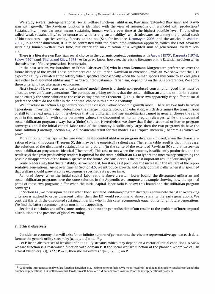
Fig. 1 illustrates the Turnpike Theorem. The solution path determined by initial conditions off ray has constant utility,and it has the property that, along this path, the sequence converges to a point in .


Fig. 1. Convergence to ray .

4.2. Discounted utilitarianism: the convergence condition ϕ < 1/�

The discounted utilitarian program DU of Section 2 specializes to program DU2[ϕ, xe0, sk0], as follows, for the education

and capital economy.Program DU2[ϕ, xe0, s

k0].

max∞∑t=1

ϕt−1u(ct, x

lt

)subject to

(1 − ı)skt−1 + it ≥ skt , t ≥ 1,

f(skt , x

ct

)≥ ct + it, t ≥ 1,

� xet−1 ≥ xet + xct + xlt, t ≥ 1.

Note that whether or not DU2[ϕ, xe0, sk0] converges depends only on ϕ and the initial ‘capital–labor ratio’ � = sk0/xe0, by

the homogeneity of the program. (The set of feasible paths is a convex cone.) We are interested in understanding the set{(ϕ,�)|DU2[ϕ, xe0, �x

e0] converges

}.

Theorem 5.

A. If ϕ� > 1, then Program DU2[ϕ, xe0, �xe0] diverges for all

(xe0, �x

e0

)∈ �2++.

B. If ϕ� < 1, then Program DU2[ϕ, xe0, �xe0] converges for all (xe0, �x

e0) ∈ �2++.


Theorem 5 is important for our theory, and perhaps surprising, for it says that the ‘power’ of the economy, in the sense ofits capacity to cause the DU2 program to diverge, depends only on the efficiency of the educational technology, namely, thecoefficient �. In particular, we need no special assumptions on the technology f other than the standard ones in AssumptionA.

The proof of Theorem 5 is not particularly transparent, and so we provide here a more intuitive argument. Let xe0 = 1.Suppose we can find positive numbers (�, c, i, xc, xl) such that the following equations hold for some given positive g:

(g + ı)� = i, (7)

f (�, xc) = c + i, (8)

� = 1 + g + xc + xl. (9)

Then, from an initial endowment of (xe0, sk0) = (1, �), we can produce a balanced growth path in which all variables grow by a

rate g at each period. Just notice that the investment defined by (7) will make sk1 = (1 + g)�, that Eq. (9) says that xe1 = (1 + g)xe0,and that the solution (c, i, xc, xl) will grow at rate g from date one onwards, invoking the fact that all three equations are


homogeneous of degree one in the five variables. Now, in order to solve these equations, it is obviously necessary that1 + g < �, for otherwise (9) would have no positive solution for (xc, xl). The interesting fact is that the converse is true aswell: as long as 1 + g < �, we can produce the required solution, which would support a balanced growth path at growthrate g beginning at a capital–labor ratio �. To see this, eliminate i using (7) (which will surely be positive for any positive �);then we must find (�, c, xc, xl) positive such that:

f (�, xc) = c + (g + ı)�,� − (1 + g) = xc + xl,

which is equivalent to finding (�, xc) such that

f (�, xc)> (g + ı)�,0< xc < � − (1 + g).

But this can be accomplished if and only if there exists � > 0 such that

f (�, � − (1 + g))> (g + ı)�,or, invoking the fact that f is one-homogeneous, if and only if:

f

(1,� − (1 + g)

�

)> g + ı.

But since f increases without bound as we increase its labor argument, we can surely find � sufficiently small that this istrue. Let the value of such an admissible � be denoted �.

Now beginning with an arbitrary positive endowment vector (xe0, sk0), we can reach the capital–labor ratio � in a finite

number of steps; from there we take off at any desired growth rate g < � − 1. Since utility is also homogenous of degree onein (c, xl), it grows at that rate too. So the growth factor of utility is (1 + g)< �. It is now clear that Program DU2 diverges ifand only if ϕ� > 1.

The reason the above argument is only an intuition for, rather than a proof of, Theorem 5, is that a proof cannot limititself to studying only balanced growth paths.

We remind the reader that Theorem 5 depends, as well, on our assumption that the leisure argument of the utility functionis measured in quality units, one that we strongly defend, although it may be somewhat controversial.

4.3. The divergence of discounted utilitarianism and the sustainability of the extended Rawlsian path

Consider the Extended Rawlsian EO, i.e., with vNM utility function given by (6) above, with ˇ∈ [0,1]. Her optimizationprogram for the education and capital economy can be written as follows.

Program Rˇ[ϕ, xe0, sk0].

max{u1 + ϕ(1 + ˇ) min {u1, u2} + ϕ2(1 + 2ˇ) min {u1, u2, u3} + · · · }subject to ut ≡ u

(ct, xlt

)and

(1 − ı)skt−1 + it ≥ skt , t ≥ 1,

f (skt , xct ) ≥ ct + it, t ≥ 1,

�xet−1 ≥ xet + xct + xlt, t ≥ 1.

Lemma 4. For any path (u1, u2, . . .) ∈ �∞+ , the sum∑∞

t=1ϕt−1(

1 + (t − 1)ˇ)

min {u1, . . . , ut} converges.


Lemma 5. If (u1, u2, . . .) solves Program Rˇ[ϕ, sk0, xe0], then ut ≥ ut+1 for all t.

Proof. Suppose to the contrary that u2 > u1. Then it follows that u1 = min{u1, u2}. We can distribute back a small amountof resources from date 2 to date 1: reduce by a small amount ε the value of xe1, increase xl1 by ε, and decrease xl2 by �ε, makingthe date 2 agent take the reduction of his skilled labor supply entirely in a reduction of leisure. This will increase the valuesof u1 and (1 + ˇ) min{u1, u2} and will leave all other numbers

(1 + (t − 1)ˇ

)min {u1, . . . , ut} unchanged or possibly greater.

Hence, since the objective was finite by Lemma 4, it is now increased, a contradiction. The general claim follows from aninduction argument. �

We now state our main theorem:

Theorem 6. Let (xe0, sk0) ∈ . If ϕ� ≥ 1, then for ˇ∈ [0,1], any solution to Program Rˇ[ϕ, xe0, s

k0] is the solution to Program

SUS2[xe0, sk0]. Since the solution to SUS2[xe0, s

k0] is unique, so is the solution to Rˇ[ϕ, xe0, s

k0].



Combined with Theorem 5, we have that, if Program DU2 diverges, then the Extended Rawlsian EO can ignore uncertaintyin choosing the optimal path (at least in the case when the initial endowment vector lies on the ray ). We conjecture thatTheorem 6 is true even if the initial endowment is not on the ray .

4.4. The case where discounted utilitarianism converges

This section focuses on the case ˇ = 0, for which Program Rˇ is just the application of the Rawlsian Program R of Section2 above to the education and capital economy: let us refer to it as Program R2[ϕ, xe0, s

k0], or simply Program R2. We expect

that, if ϕ� < 1, then the solution to Program R2 will not be the solution to Program SUS2, which is to say that the inequalitiesut ≥ ut+1 of Lemma 5 will not all be satisfied with equality. Thus, the solution to the Rawlsian EO’s problem under uncertaintyR2 may involve decreasing utilities over time. Indeed this is true for ϕ sufficiently close to zero, as the following simple resultshows.

Theorem 7. Given (xe0, sk0), there is a number ϕ > 0 such that, if ϕ < ϕ, then the solution to R2[ϕ, xe0, s

k0] entails u1 > u2 on the

solution path.


Moreover, a consequence of Theorem 8 below is that, under our Cobb-Douglas assumptions, for any ϕ < 1/�, if thecapital–labor ratio sk0/x

e0 is sufficiently high, then utilities are strictly monotone decreasing on the optimal path.

We now ask: If the DU2[ϕ, xe0, sk0] program converges, is its solution the same as the solution to R2[ϕ, xe0, s

k0]? By Lemmas

1 and 5, this will be the case if, at the solution to DU2[ϕ, xe0, sk0], utilities are weakly decreasing with time.

For an initial condition (sk0, xe0), define the ‘capital–labor ratio’ �0 = sk0/xe0. Recall that u(c, x) = c˛x1−˛, and f (s, x) = sx1− .

Define the following variables:

E = (ϕ�)1/(˛)(1 − ı),

xc1 = (� − E)˛(1 − )1 − ˛ , xl1 = (� − E)(1 − ˛)

1 − ˛ , xet = Et,

c1 = �0(xc1)1−(1 − ı),

skt = (1 − ı)tsk0, xct = xc1Et−1, xlt = xl1Et−1, ct = c1((1 − ı)E1−)t−1.

Theorem 8. Suppose that ϕ� < 1, and that sk0/xe0 = �0 ≥ �∗ where �∗ is the root of the equation

1 − (

xc1(1 − ı

)�

)1−

= c1

xl1

(ϕ�)1/(˛) (1 − ˛)

�(

1 − ˛) .

Then the solution to DU2[ϕ, xe0, sk0] is given by the geometric sequence: skt = skt xe0, xet = xet xe0, xlt = xltxe0, xct = xct xe0, it = 0 for all

t ≥ 1.


Corollary. If ϕ� < 1 and �0 ≥ �∗, then Programs DU2[ϕ, xe0, sk0] and R2[ϕ, xe0, s

k0] are equivalent.

Proof. Along the solution to Program DU2, we have that

ut = u1

(((1 − ı

)E1−

)˛E1−˛

)t−1

,

where u1 = c˛1 (xl1)1−˛

; thus utilities are strictly decreasing with time because E < 1. The result then follows from Lemmas 1and 5. �

What happens when �0 < �∗? The solution to DU2 will not be the well-behaved solution of geometric decay of Theorem8. Will, nevertheless, utilities still be monotone decreasing on the optimal path? Perhaps, surprisingly, the answer is ingeneral negative. Example 2 in Appendix A has the property that, along the solution path to Program DU2, u2 > u1, whereasthe utilities from date 2 onwards decay geometrically as in Theorem 8.

How do the solutions to DU2 and R2 compare when they are different and DU2 converges? To see this, we calculatethe solution to R2 for Example 2 in Appendix A. There, the Rawlsian EO gives higher utility to the first generation than theutilitarian EO, but the reverse is true for all dates after that. In fact, the ratio of utilities for the two programs is constant fordates 2 and later at 1.015, with the larger utility associated with DU2: this is perhaps a surprise.


This concludes our discussion of the relationship between the DU2 and R2 programs in the case where DU2 converges.Unlike the cake-eating problem, the solutions to these two programs are not always identical – although they are identicalwhen the initial capital–labor ratio is sufficiently large.

Based on Example 2 in Appendix A, we may conjecture what the general solution to DU2[ϕ, xe0, sk0] looks like in the

convergent case. There will be a sequence of numbers � > �∗ > �1 > �2 > · · ·> 0, where �∗ is given in Theorem 8, where,if �T > �0 > �T+1, the first T dates will have it > 0, and at date T + 1, the capital–labor ratio will be �, at which point thegeometric-decay solution of Theorem 8 takes over. The same pattern should be true in the solution to Program R2[ϕ, xe0, s

k0],

except that utility will be equal for all the dates when investment is positive.

4.5. Growth

Some may find sustainability, in the sense of program SUS, to be too stark, as it leads to a constant level of human welfareuntil the disappearance of the species. If, however, we treat resources, such as the biosphere, as of limited capacity, thensustainability may be the best we can hope for. Nevertheless, we now introduce a program which permits the growth ofwelfare.

Program g-SUS[xe0, sk0].

max� subject to

[(rt)] u(ct, xlt) ≥ (1 + g)t−1�, t ≥ 1,

[(at)] f (skt , xct ) ≥ ct + it, t ≥ 1,

[(bt)] (1 − ı)skt−1 + it ≥ skt , t ≥ 1,

[(dt)] �xet−1 ≥ xet + xct + xlt, t ≥ 1.

Program g-SUS maximizes date-1 welfare subject to assuring that welfare grows at rate g forever. Obviously, Program g-SUSbecomes SUS2 when g = 0.

What is the largest g for which Program g-SUS possesses a solution? We give a partial answer with the next theorem.Definition. A balanced growth path at rate g is a path satisfying the (at), (bt) and (dt) constraints of Program g-SUS[xe0, s

k0]

such that:

skt = (1 + g)skt−1 and xet = (1 + g)xet−1, for t ≥ 1,

zt = (1 + g)zt−1 for all other variables z ∈{xc, xl, i, c

}, for t ≥ 2.

Theorem 9. Suppose that 0 ≤ g < � − 1 and xe0 = 1. Then there exists a value sk0 such that the solution to Program g-SUS[xe0, sk0]

is a balanced growth path at rate g. Conversely, if g ≥ � − 1, then there exists no such path for any value of sk0.6

Proof. Appendix A.�

We expect that a turnpike theorem holds for the g-SUS model as well, and so, if and only if 0 ≤ g < � − 1, and given anyvalue of sk0, Program g-SUS will possess a solution at which all constraints bind, which converges to a balanced growth pathat rate g.

4.6. Social choice when DU2[ϕ, xe0, sk0] diverges

According to Theorem 5, DU2[ϕ, xe0, sk0] diverges when ϕ� > 1. The usual way of choosing among paths in the case of

divergence is to use a version of the overtaking criterion: the latest proposal that we have seen along these lines is thatof Basu and Mitra (2007). The utility path ( ¯u1, ¯u2, . . .) is at least as good as the utility path (u1, u2, . . .) according to theovertaking criterion if there exists a T such that

∑T−1t=1 ϕ

t−1 ¯ut ≥∑T−1

1 ϕt−1ut and t ≥ T ⇒ ¯ut ≥ ut . This defines a pre-order (i.e., an incomplete order) on feasible paths when a program diverges.

The proof of Theorem 9 showed that balanced growth paths exist for the education and capital economy as long asg < � − 1. The condition for a divergence of such a path in Program DU2 is ϕ(1 + g) ≥ 1. This condition surely holds when gis close to � − 1 because ϕ(1 + (� − 1)) = ϕ� > 1.

Let (u1, u2, . . .) and ( ¯u1, ¯u2, . . .) be two feasible balanced-growth paths for a given initial endowment (xe0, sk0) which grow

at rates g1 and g2, respectively, where g2 > g1. It is easy to see that ( ¯u1, ¯u2, . . .) is better than the utility path (u1, u2, . . .)according to the overtaking criterion. But it is also the case that utility will be smaller for the early date(s) on the preferredpath. (To grow forever faster requires making early sacrifices.) This is interesting, because discounted utilitarianism is usuallyassociated with implying that the later generations sustain low utility. This, however, is only the case when the program

6 We are not interested in the problem with negative g.


converges. Indeed, as the proof of Theorem 9 shows, as the growth rate g approaches its unattainable supremum (� − 1)(and these high-growth-rate paths are the most desirable paths according to the overtaking criterion), the utility of thefirst generation approaches zero. We do not take this as a criticism of overtaking: rather, it is a criticism of discountedutilitarianism.

In contrast, as Theorem 6 showed, if ϕ� ≥ 1, then the solution to Program R2[ϕ, xe0, sk0] entails constant utility for all

generations, at the highest possible level at which such a level can be sustained. We find this distinctly superior, from theethical viewpoint, to the recommendation of the discounted utilitarian.

Finally, we note that the case of divergence may be the salient one. By definition, � = xt/xet−1 = xt/ (�ext−1), where �e is thefraction of the labor force of generation t − 1 that is devoted to teaching. As a rough approximation, assume that populationgrowth is zero and that skill growth is zero; then xt = xt−1 and so, if �e ≈ 0.05, we have � ≈ 20. Since we have suggested,following Stern (2007), that ϕ = 0.999 is appropriate, we have that ϕ� is substantially larger than one.

5. Conclusion

In the cake-eating problem, we showed that two Ethical Observers, facing uncertain possible future worlds, who haveutilitarian and Rawlsian von Neumann Morgenstern preferences over risk, respectively, would recommend the same allo-cation of the exhaustible resource over future generations. At first blush, it seems surprising that these two Observers, withapparently very different preferences, would agree on the recommended path. The best analogy we can think of is withthe solution to the problem with no uncertainty concerning the existence of future generations, and a finite horizon. Theutilitarian and the Rawlsian will recommend the same allocation of the exhaustible resource in this case – namely, splitit equally among all generations. This solution is unique only if u is strictly concave – if u is linear, then the utilitarian isindifferent among all possible distributions of the resource.

We then introduced a generalization of the classical growth model, which includes an education sector. Moreover,we postulated that welfare depends on consumption and educated leisure. Now, the program of the utilitarian EthicalObserver, in the presence of uncertainty, does not always converge, while the program of the sustainabilitarian (i.e., Rawl-sian) does. We characterized when the former program converges (Theorem 5), and we showed that when it does notconverge, the (extended) sustainabilitarian proposes the same path as she would if there were no uncertainty (Theorem6). We believe this is an important result, as parameter values in the real world are likely to be such that the discountedutilitarian program does not converge (see Section 4.6). Moreover, we argued that if this is the case, then the most desir-able paths according to the discounted-utilitarian objective would leave the early generations with very low utility. (Thisconclusion is very different from the recommendation of discounted utilitarianism in the convergent case.) In contrast,when the discounted utilitarian program diverges, as we said, the sustainabilitarian recommends equal welfare for allgenerations.

Finally, we showed that when the discounted utilitarian program converges, it is not generally the case that the twoEthical Observers will recommend the same paths, although they do if the capital–labor ratio of the initial endowmentvector is sufficiently large (Theorem 8 and its Corollary).

In our companion paper Llavador et al. (2010), we study a model which is a ramification of the model of Section 4 of thepresent paper, one which articulates the issue of global warming. In that model, production of the consumption-investmentgood affects negatively the quality of the biosphere (carbon emissions increase global temperature), and the quality of thebiosphere enters into the utility of individuals. As well as a production and education sector, that model also contains anR&D sector, where research produces knowledge that both improves the technology of commodity production, and entersdirectly into the utility of people. (Knowledge and biospheric quality are global public goods.) We know that with appro-priate parameter values, the discounted utilitarian program of the more ramified model diverges; we do not know whetheranalogues of the theorems presented here continue to hold. Naturally, we would be interested in eventually extending thepresent analysis to that model: we propose to think of the central results of the model of Section 4 as conjectures concerningthe global-warming model. In particular, if the discounted-utilitarian objective function diverges on the set of paths definedfor the global-warming model, then we conjecture that the sustainabilitarian can ignore the kind of uncertainty studied inthe present paper (Theorem 6). However, we must say that there is another kind of uncertainty, not discussed here, whichis more the focus of current discussions of global warming: the uncertainty about the relationship between atmosphericcarbon and global temperature (biospheric quality). That kind of uncertainty involves quite different considerations fromthose studied here.

Acknowledgements

We are indebted to a referee for detailed and useful suggestions. Klaus Nehring, Andreu Mas-Colell and Geir Asheimprovided helpful comments. We thank the audiences in various presentations, in particular in the European General Equi-librium Workshop in Honor of Andreu Mas-Colell, Barcelona, June 2009. We also thank Cong Huang for his collaborationon the proof of the Turnpike Theorem. The usual caveat applies. Financial support from the BBVA Foundation is gratefullyacknowledged.


Appendix A. Proofs and Examples

Proof of Lemma 3. We claim that for every T, yRT = min{yR1, yR2, . . . , yRT }. For suppose this were not the case, for some T. Thenlet ε = yRT − min{yR1, yR2, . . . , yRT−1}. By hypothesis, ε > 0. Define the path (y1, y2, . . .) as follows:

yT = yRT − ε

2,

yt = yRt + ε

2(T − 1), for 1 ≤ t ≤ T − 1,

yt = yRt , for t > T.

Obviously (y1, y2, . . .) is feasible for Program R1. In the move from (yR1, yR2, . . .) to (y1, y2, . . .), the first T terms in the objective

function of Program R1 all (strictly) increase. Furthermore, all terms greater than the T th term either increase or stay thesame. Notice that yT remains at least ε/2 greater than the minimum of {y1, y2, . . . .,yt} for all t > T , since that minimum isbounded above by min{y1, . . . , yT−1}. So u(yT ) is never the minimum in any of the terms of the objective with t > T . Conse-quently, the objective function of Program R1 (obviously bounded) attains a higher value at (y1, y2, . . .) than at (yR1, y

R2, . . .),

a contradiction.�

Proof of Theorem 2.

Step 0. Since u(0) is finite, w.l.o.g., we take u(0) = 0.Step 1. Let (yDU1 , yDU2 , . . .) solve Program DU1. Suppose there is a T such that yDUt = 0. Then T must be greater than one. For ifyDU1 = 0, simply define a new path (y1, y2, . . .) by yt = yDUt+1 for all t = 1,2, . . . This path increases the value of the objectivefunction in DU1, an impossibility. Therefore T > 1.Step 2. Now let T be the smallest date for which yDUt = 0. Then it must be the case that for any sufficiently small ε > 0,we have u(yDUT−1 − ε) + ϕu(ε) ≤ u(yDUT−1), for otherwise, a transfer of ε from date T − 1 to date T would increase the valueof the objective function in Program DU1. But this inequality can be written ϕu(ε) ≤ u(yDUT−1) − u(yDUT−1 − ε). Dividing both

sides by ε and letting ε approach zero, this implies that ϕ lim u(ε)ε ≤ u′(yDUT−1). But lim

ε→0

u(ε)ε = ∞, which gives the desired

contradiction.�

Example 1

This is an example of a function u for which Program DU1 has no solution. Consider the function u : �++ → � : u(y) =∫e1/ydy− y. We have u′(y) = e1/y − 1, u′′(y) = − e1/y

y2 . Thus, u is an increasing, concave function on the positive real line,

and the Inada condition holds. The function u cannot be continuously defined at zero, as it approaches negative infinity as yapproaches zero.

If the path(yDU1 , yDU2 , . . .

)solves problem DU1 for this u, then

(yDU1 , yDU2 , . . .

)must be strictly positive because

the domain of u is �++. It follows that the first-order Kuhn-Tucker conditions hold – there is a number � > 0 suchthat e1/yt = 1 +

(�/ϕt−1

)for all t. But this implies that yt = 1/ log

[1 + �/ϕt−1

], and so it must be the case that∑∞

t=1

{1/(

log[1 + �/ϕt−1

])}= 1. For large t, we can approximate the denominator in the terms in this series by

log�/ϕt−1 = log�+ (t − 1) log(

1/ϕ)

. But these terms grow like k(t − 1), where k = log(1/ϕ), and so the series grows like1/ (k(t − 1)), and therefore it does not converge, a contradiction. Therefore there is no solution to program DU1, and henceto the Program R1, for this u.

The intuition here is that the derivative of u is increasing too fast (exponentially) as y approaches zero. LetVR (y1, y2, . . .) be the value of the objective function of Program R1 at path (y1, y2, . . .). The result is perhaps sur-prising, because it is easy to see that the function VR (y1, y2, . . .) is bounded on the feasible set. Hence, it mustbe the case for this u that the finite supremum of

{VR(y1, y2, . . .)|(y1, y2, . . .) is feasible

}is never attained. It is

easy to check that if u(y) = yr/r, for any r ∈ (−∞,1), then Program DU1 has a solution. The Inada condition holdsfor these functions, and the first order-conditions can be solved for a positive path whose components sum tounity.


Proof of Theorem 3.

Step 1. We introduce the following sequence of programs. Define Program DUT as:

maxT∑t=1

ϕt−1u(yt)

subject toT∑t=1

yt ≤ 1,

yt ≥ 0,∀t ≥ 1.

Step 2. Note that for sufficiently large T, it must be the case that the solution (z1, z2, . . . , zT ) to ProgramDUT , which of courseexists, has zT = 0. For if not, and (z1, z2, . . . , zT ) � 0, then there are first order conditions of the form:

ϕt−1u′(zt) = �, some positive number�.

Of course it follows, from the usual argument, that (z1, z2, . . . , zT ) is a weakly decreasing sequence, and consequently, bychoosing a large T, we can guarantee that zT is bounded above by an arbitrarily small number, because of the cake-eatingconstraint. Consequently � must be very close to ϕT−1� , and hence must be arbitrarily small. But since u′(z1) = �, thisimplies that z1 becomes arbitrarily large, contradicting the fact that

∑zt = 1. Thus there is a date T such that the solution

to Program DUT has zT = 0.Step 3. Now let T be the smallest date such that zT = 0; denote the solution to Program DUT by (z1, z2, . . . , zT ). We willassume that zt > 0 for t < T , but the proof can be modified in an obvious way if this is not the case. Then the followingKuhn-Tucker (K-T) conditions must hold for the (concave) Program DUT :

There are non-negative numbers �, T such that:

ϕt−1u′(zt) − � = 0, for t < T,

ϕT−1� − �+ T = 0.

Step 4. We claim that the path zT+1 ≡ (z1, . . . , zT ,0) is the solution to Program DUT+1. To see this, write down the K-Tconditions for this program, namely:

There are non-negative numbers (�, T, T+1) such that:

ϕt−1u′(zt) − � = 0, for t < T,

ϕT−1� − �+ T = 0,

ϕT� − �+ T+1 = 0.

We note that the values of � and T continue to solve these FOCs, for the vector zT+1, and we define the new shadowprice by

T+1 = �− ϕT� > 0.

Thus, since we have a concave program, we have shown that zT+1 is its solution.Step 5. We continue in this manner to show that the vector zS = (z,0,0, . . . ,0) is the solution to ProgramDUS for any S > T .The new Lagrangian multiplier at each step is defined by:

S = �− ϕS−1�,

and so we note, for use below, that limS→∞ S = �.


Step 6. We now claim that the vector (z∞1 , z∞2 , . . .) ≡ (z,0,0, . . . .) solves ProgramDU1. We proceed by contradiction. Denote

by VDU(y1, y2, . . .) the value of the objective function of Program DU1 at the path (y1, y2, . . .). Suppose the claim were false,and there is a path (y1, y2, . . .) with VDU (y1, y2, . . .)> VDU

(z∞1 , z

∞2 , . . .

). Write yt = z∞t + gt for all t; of course,

∑gt = 0.

We define a function H : � → � as follows:

H(ε) =T−1∑t=1

ϕt−1u(z∞t + εgt) +∞∑t=Tϕt−1u(0 + εgt) + �

(1 −

∞∑t=1

(z∞t + εgt))

+∞∑t=T t(0 + εgt).

Verify thatH(0) = VDU(z∞) and thatH(1) ≥ VDU(y1, y2, . . .), which follows from the fact that (y1, y2, . . .) is feasible and thatthe Lagrangian multipliers are all non-negative. Suppose we can show that H is maximized at zero: then we will know thatH(0) ≥ H(1), which implies that VDU (z∞) ≥ VDU (y1, y2, . . .), which is the desired contradiction.Step 7. It therefore remains to show that zero maximizes H. Note that H is a concave function, so it suffices to show thatH′(0) = 0. We compute:

H′(0) =T−1∑t=1

ϕt−1u′(z∞t )gt +∞∑t=Tϕt−1�gt − �

∞∑t=1

gt +∞∑t=T tgt.

Grouping together all terms associated with the same gt , we see that for t < T , the coefficient of gt is ϕt−1u′(z∞t ) − � = 0,and for t ≥ T the coefficient of gt is ϕt−1� − �+ t = 0. Thus the derivative vanishes at zero, as required.Step 8. There is a final, transversality condition: We must show that the function H is well-defined on the interval [0,1].The only term that might cause concern is the last one, which is ε

∑∞t=1 tgt . But since t → � and gt → 0 and

∑∞t=Tgt =

−∑T−1

t=1 gt , it follows that∑∞

t=1 tgt converges, and the proof is complete.Step 9. The uniqueness of the solution follows from the strict concavity of u.�

Proof of Theorem 4 (The Turnpike Theorem).The programRecall that we aim at finding the maximum level of sustainable utility for a fairly simple infinitely lived economy. Formally:Program SUS2.

max� subject to

(P1) c˛t (xlt)1−˛ ≥�, t ≥ 1,

(P2) �xet−1 ≥ xet + xlt + xct , t ≥ 1,

(P3) (skt )(xct )

1− ≥ ct + it, t ≥ 1,

(P4) (1 − ı)skt−1 + it ≥ skt , t ≥ 1.

The initial endowment is a vector (xe0, sk0).

The value function of the program maps the initial endowment into the value�; thus we write V(xe0, sk0) =�.

Define F� = {(xe0, sk0)|V(xe0, s

k0

)=�}. This is the set of initial endowments that generate the same value for SUS2.

We define a feasible path as a set of sequences {xet }t=0,1,2...., {skt }t=0,1,2.... and all other variables beginning at t = 1, suchthat inequalities (P2), (P3), and (P4) hold. Denote the set of feasible paths by P.

Denote the set of feasible paths beginning at a given initial vector (xe0, sk0) by P(xe0, s

k0).�

Proposition 1. The set P is a closed convex cone. The set P(xe0, sk0) is closed and convex.

Proof. Easy.�

Proposition 2. At any solution to Program SUS2, all the constraints (P1)–(P4) bind at all dates. The solution to SUS2 is unique.

Proof.

Step 1. It is obvious that (P2)–(P4) bind. What requires proof is that u(ct, xlt) =� for all t. We first prove this is the case fort = 1. Suppose, to the contrary, that at an optimal solution, u(c1, xl1)>�. Reduce xl1 by ε and increase each of xe1 and xc1 by


ε2 so that u(c1, xl1 − ε) ≡�′ >�. Now define

(i′1, s

k′1

)to be the simultaneous solution of the two equations:

c1 + i′1 = f(sk

′1 , x

c1 + ε

2

),

(1 − ı)sk0 + i′1 = sk′1 .

Obviously, sk′

1 > sk1; therefore (xe1 + ε

2 , sk′1 ) � (xe1, s

k1). It follows that, with this altered vector of endowments, (xe1 + ε

2 , sk′1 ),

for the program beginning at date 2, the value of the program beginning at date 2 is greater than�, since the value functionof the program is homogeneous of degree one in its endowment vector. Let the value of the program, beginning at date 2,be �∗ >�. We have now produced a feasible path where for all t, u(ct , xlt) ≥ min(�′,�∗)>�. This contradiction provesthat u(c1, xl1) =�.Step 2. Assume now that in any optimal solution, for 1 ≤ t < T , u

(ct, xlt

)=�, but there is an optimal solution for which

u(cT , xlT )>�. Reduce xeT−1 by ε/� and increase xlT−1 by the same amount, increasing utility at date T − 1, which is now

greater than �. This decreases xT ≡ xeT + xlT + xcT by ε, and let this decrease be implemented by decreasing xlT by ε, whichmay be chosen small enough that utility at date T is still greater than �. We have now produced an optimal path for theprogram for which u(cT−1, x

lT−1)>�, which contradicts the induction hypothesis. This proves that for all t, ut =�.

Step 3. We next show that the solution to SUS2 is unique. Any two solutions must have the same values of {(ct, xlt)}: for if not,take any non-trivial convex combination of the two solutions, producing another optimal solution for which the constraints(P1) do not bind (using the Cobb-Douglas form of u); this contradicts what has been proved above. In like manner, the values{(xet , skt )} must be the same in the two solutions, since otherwise a convex combination of them would produce an optimalsolution in which the constraints (P3) do not bind. But if the dated capital-stocks are identical in the two solutions, so mustbe the dated investments. Since the values {(xct , xlt)} are identical in the two solutions, we see, by iteration, that the valuesof {xet } are also identical. This proves the claim.�

Proposition 3.

A. Let (xe0, sk0) � (xe0, s

k0). Then V(xe0, s

k0) � V(xe0, s

k0).

B. Along the optimal path beginning at (xe0, sk0), there is no T such that (xeT , s

kT ) � (xe0, s

k0).

C. Let (xe0j, sk0j) ∈ F� be an infinite sequence of points in F� , for some fixed �, such that xk0j → ∞. Then sk0j → 0.

Proof.

A. If (xe0, sk0) � (xe0, s

k0), then there is a positive number ı∗ such that (xe0, s

k0) � (1 + ı∗)(xe0, s

k0). Since P is a cone, and the utility

of Generation t is homogenous of degree 1 in its arguments, it follows immediately that V(xe0, sk0)> (1 + ı∗)V(xe0, s

k0).

B. Suppose that there is a T such that (xeT , skT ) � (xe0, s

k0). Let the value of the program be �. By Part A, the value of the sub-

program that begins at date T is strictly greater than �. This contradicts the fact that the constraints (P1) are binding for allt.C. Suppose the premise were false; then there is a subsequence sk0j → S > 0, some S. We can choose a number S > S and a

number x such that V(x, S) = � > �. We can also choose an index j such that the program beginning with the endowments(xe0j, s

k0j) possesses a feasible path that, at its first step, has three properties:

(i) sk1 > S,(ii) xe1 > x,

(iii) c˛1 (xl1)1−˛

> �.

(This is obvious from examining the technology.) It therefore follows that V(xe1, sk1)> �: invoke Part A of this proposition.

But this is a contradiction, because V(xk0j, sk0j) = � < �. �


Since all the constraints of SUS2 bind, we can write down the Kuhn-Tucker conditions for this concave program. It turnsout that these conditions imply only three new pieces of information, which are:

(D1)xltct

= 1 − ˛˛(1 − )

xctct + it , t ≥ 1;

(D2)xlt+1

ct+1= xltct

�

1 − ı

(1 − (ct + it)

skt

), t ≥ 1.

(D3)∑t

(1�

)txlt converges.

The other Kuhn-Tucker conditions just define the various Lagrangian multipliers, which are all non-negative.It follows that: A feasible path and a number � for which all the primal constraints bind at all t, and for which (D1),(D2) and

(D3) hold, is an optimal solution.7

The stationary ray

We ask: Is there a ray of initial endowments in �2+ for which the optimal solution is stationary, that is, for which allvariables are constant over time? We study this by writing down the primal constraints and equations (D1) and (D2) for ahypothetical stationary ray, and see what they imply. Indeed, we can solve them: there is a unique such ray for the initialcondition. The ray passes through the following point:

xe0 = 1, sk0 = (� − 1)

(�

� + ı− 1

) 11 −

xc∗,

where xc∗ = ˛(1 − )(� + ı− 1)˛(1 − )(� + ı− 1) + (1 − ˛)(� + ı− 1 − �ı)

.

Indeed, we can compute the values of all the variables on this ray. Call these the stationary state values. Of course they aredefined up to a multiplicative constant. Let us denote this ray by .

The Turnpike Theorem

It is very difficult to actually compute the optimal path, if we begin from an endowment vector off the stationary ray .We shall, however, prove (Proposition 4) that from any initial vector (xe0, s

k0), the optimal solution to SUS2 converges to a

point on .In the following, given any two variables at and bt , we use the notation for ratios: atbt =

(ab

)t.

Lemma 6. Suppose that, in the optimal solution, the limit of the sequence {(xl/c)t=1,2,...} exists and is finite. Then the solutionconverges to the stationary state values.

Proof.

Step 1. Denote the limit of the sequence {(xl/c)t=1,2,...} by �. We first argue that � /= 0. If � = 0, then lim (c/xl)t = ∞. By

(D1), lim (xc/(c + i))t = 0, and so lim (xc/sk)t = 0, by invoking (P3). Now (ct + it)/skt = (xct /skt )

1−, so lim (ct + it)/skt = 0,

which means, by (D2), that (c/xl)t+1/(c/xl)t → ((1 − ı)/�)< 1, because � > 1. It is therefore impossible that lim (c/xl)t = ∞.Therefore � > 0.Step 2. By (P1), xlt(ct/x

lt)˛ = � for all t. Therefore lim xlt = ��˛ and so lim ct = ��˛−1. From (D2), it also follows that

�1−ı lim

(1 − (ct+it )

skt

)= 1; therefore lim

((c + i)/sk

)t

has the value of the ratio of (c + i)/sk in the stationary state. Therefore

lim (xc/sk)t has the same value as the ratio of those variables in the stationary state. By (D1) it now follows that � is alsothe ratio of xl/c in the stationary state.Step 3. Suppose that there were a subsequence of {skt } that diverged to infinity. Since lim (xc/sk)t is finite, it follows that thesame subsequence of {xct } diverges to infinity. It follows from (P2) that the same subsequence of {xet } diverges to infinity. Inparticular, there exists a T such that (xeT , s

kT ) � (xe0, s

k0). But this contradicts Part B of Proposition A.3. Therefore the sequence

{skt } is bounded. It immediately follows that the sequence {xct } is bounded, since lim (xc/sk)t exists and is finite; and sincelim ((c + i)/sk)t also exists and is finite, the sequence {it} is bounded.

7 One may ask, conversely: Does the optimal solution have to satisfy these equations? The answer to this must be affirmative: there is an infinitedimensional version of the Kuhn-Tucker theorem, using the Hahn-Banach theorem, which tells us that this is so.


Thus all the sequences of variables, except possibly for {xet }, are bounded. Therefore we can choose a single subsequenceof all the variables (except possibly of {xet }) which converges to values (sk, xc, i) and we have already shown that {xlt}, {ct}converge to values xl and c. Furthermore we know that {skt } converges to a positive number, because lim((ct + it)/skt ) hasthe value of the same ratio in the stationary state and {ct} converges to a positive number.

It now follows, by invoking Proposition A.3, Part C, that {xet } does not diverge to infinity – since (xet , skt ) ∈ F� for all t. So

there is a subsequence of the original sequence such that all variables converge.We proceed to show that this subsequence of variables converges to stationary state values. Denote the limits:

�1 = limct + itxct

= limc + itxct

, (A.1)

�2 = lim

(sk

xc

)t

. (A.2)

We have shown that �1 and �2 are the values of the corresponding ratios in the stationary state. Now from (P3) we have:

xct �2 − it → c. (A.3)

Note that Eqs. (A.1) and (A.3) comprise two simultaneous equations, in the limit, for the limits of the variables xc and i.Hence the sequences {xct } and {it} must converge, and to stationary state values, since these same two equations hold forthe stationary state variables. We therefore have, by (A.2), that {skt } also converges to the appropriate stationary state value.Likewise with {xet }.

Finally, indeed the whole sequence of variables converges to the same stationary state: for if not, there would be anotherlimit point approached simultaneously by some other subsequence of the variables, to a stationary state. But since thestationary ray is unique, that limit of (xet , s

kt ) must also be on the ray . However, we cannot have two subsequences

approaching different points on the ray: that would violate Proposition A.3, Part B.�

Proposition 4. From any initial vector (xe0, sk0), the optimal solution to SUS2 converges to a point on .

Proof. 8

Step 1. On the optimal path, the sequence {( xlc )t=1,2,...} does not diverge to infinity. Suppose it did diverge to infinity. Then

from (D1), the sequence xct / (ct + it) diverges to infinity also. But, invoking (P3), xct / (ct + it) = (xct /skt ), and so xct /s

kt → ∞.

Now (ct + it)/skt = (xct /skt )

1−, and so it follows that (ct + it)/skt diverges to infinity. But this contradicts (D2), for it would

mean that eventually the ratio xlt/ct is negative.

Step 2. Hence it follows that, on the optimal path, the sequence {( xlc )t=1,2,...} has a (finite) limit point. If the sequence

{( xlc )t=1,2,...} indeed converges to this limit point, then the theorem is proved, by Lemma A.6.

Step 3. Thus, the remainder of the proof will show that the limit point of the sequence {( xlc )t=1,2,...} is unique, and hence itis the limit of the sequence.

By exploiting equations (D1) and (P3), we can rewrite (D2) as follows:

(D2∗)

(xl

c

)t+1

=(xl

c

)t

�

1 − ı

(1 −

(˛(1 − )

1 − ˛

) 1−(xl

c

) 1−

t

).

It will be convenient to define the function: f ∗(x) = ax(1 − bxr), where a = �1−ı , b =

(˛(1−)

1−˛

) 1−

, and r = (1 − )/. Thus

(D2∗) says that

f ∗(xctct

)=xct+1

ct+1for all t.

Compute that d2f ∗dx2 = −rab(1 + r)xr−1, and so f ∗ is a concave function on �+. Let A∗ be the value of the ratio xl

c in the stationarystate. Then we have: f ∗(A∗) = A∗ and f ∗(0) = 0. The first claim follows since the equation (D2∗) holds, of course, at thestationary state as well.

Finally, note that another root of f ∗ is given by x∗ =(

1/b)1/r

. Concavity implies that f ∗ has only the two fixed points 0and A∗.

8 Thanks to Cong Huang, who completed and simplified this proof.


Because

{(xlc

)t=1,2,...

}is bounded, it possesses a lim inf and a lim sup. For convenience, denote yt =

(xlc

)t, and define

� = lim inf yt, �∗ = lim sup yt.

Since f ∗(yt) = yt+1, we have inf f ∗(yt) = �, and by the continuity of f ∗, inf f ∗(yt) = f ∗(inf yt) = f ∗(�) = �, so � is a fixed pointof f ∗. In like manner, �∗ is a fixed point of f ∗.

If we can establish that � /= 0, then we must have � = A∗ = �∗, and hence the limit of {yt} exists. But this is establishedby an argument that mimics Step 1 of the proof of Lemma A.6, as follows.

If � = 0, then, by (D1), lim inf(xc/(c + i)

)t= 0, and so lim inf

(xc/sk

)t= 0, by invoking (P3). Now (ct + it)/skt =

(xct /s

kt

)1−, so lim inf (ct + it)/skt = 0, which means, by (D2), that lim inf yt+1/yt = �/

(1 − ı

)> 1, because � > 1. But

this immediately implies that lim inf yt > 0, a contradiction. Therefore � /= 0, and Proposition A.4 is proved.The proof of the Turnpike Theorem follows from the previous discussion, in particular from Propositions A.2 and A.4.�

Proof of Theorem 5. Part A

Step 1. Let xe0 = 1. We claim that for any small ε > 0, we can find values � and i such that:

i = (� − ε+ ı− 1)�,i = f

((� − ε)�, ε

).

By plotting the graphs of these two functions in (�, i) space, we can observe that they cross at the origin and at some positivevalue of i– by assumption A (b).Step 2. Let ε < (ϕ� − 1)/ϕ, and let � be chosen to satisfy the equations in Step 1, thus defining investment at date 1 when

xc1 = ε, xe1 = � − ε, c1 = 0 = xl1.

Note from Step 1 that we may take sk1 = (� − ε)�. Let V(xe0, sk0) be the value function of Program DU2[xe0, s

k0], if it converges.

Then we must have, by consideration of the choice of date 1 values above, V (1, �) ≥ 0 +(� − ε

)ϕV (1, �). But

(� − ε

)ϕ >

�ϕ −(�ϕ − 1

)= 1, implying that the last equation stated cannot hold, and hence ProgramDU2 must diverge beginning with

endowment (1, �).Step 3. It immediately follows that Program DU2 diverges for � > �. (Just throw away some capital at date 1 and reducethe capital–labor ratio to �.) Moreover, the program must diverge for 0< � < � as well (at date 1, invest very little ineducation, thus increasing the capital–labor ratio at date 2 to a value sk1/x

e1 ≥ �).

Part B

Step 1. Let xe0 = 1. The largest possible investment that can be made at date 1 if sk0 = � is given by I(�), defined by theequation:

f ((1 − ı)� + I(�), �) = I(�),

because xc1 ≤ �. Define �∗ such that:

f

((1 − ı), �

�∗

)/(� − (1 − ı)) = 1 − f1((1 − ı)�∗, �),

where f1(s, x) = ∂f∂s

(s, x). A monotonicity argument, invoking the intermediate value theorem, shows that�∗ exists uniquely.Letm = f1((1 − ı)�∗, �) and note that 0< m< 1.

Step 2. The graph of the function

z(i) = f ((1 − ı)�∗ + i, �)


lies everywhere on or below the graph of the function

y(i) = f ((1 − ı)�∗, �) +mi,

and y(0) = z(0) (by the concavity of f). The second graph meets the 45◦ ray in (i, y) space at the point i = f(

(1 − ı)�∗, �)/

(1 −m). Therefore

I(�∗) ≤ f ((1 − ı)�∗, �)1 −m .

Step 3. Hence, beginning at sk0 = �∗:

sk1 ≤ (1 − ı)�∗ + I(�∗) ≤ (1 − ı)�∗ + f ((1 − ı)�∗, �)/(1 −m)

≤ (1 − ı)�∗ + �∗(� − (1 − ı)) = ��∗.

Therefore:

u(c1, xl1) ≤ u(f (sk1, �), �) ≤ u(f (��∗, �), �) ≤ �N,

where N ≡ u(f (�∗,1),1).Step 4. For any number > 1, we have:

f ((1 − ı) �∗ + I(�∗), �)< f ((1 − ı) �∗ + I(�∗), �) = I(�∗).

Consider the function � (x) = x − f ((1 − ı) �∗ + x, �); note that � ′(x)> 0 (since m < 1). We have (from the above) that� ( I(�∗))> 0, and by definition, � (I( �∗)) = 0. It follows that I( �∗)< I(�∗).Step 5. Now compute that

sk2 ≤ (1 − ı)sk1 + I(sk1) ≤ (1 − ı)��∗ + I(��∗) ≤ (1 − ı)��∗ + �I(�∗) = �((1 − ı)�∗ + I(�∗)) ≤ �2�∗,

which follows by invoking the definition of I(·), and steps 3 and 4.By induction we have skt ≤ �t�∗. But xct ≤ �t and xlt ≤ �t as well, and so u

(ct, xlt

)≤ u(f(skt , �

t), �t)

≤ �tN. It follows that∑ϕt−1ut ≤ �∑(

ϕ�)t−1

N <∞.

Step 6. Now suppose that � > �∗; let � = �∗, > 1. Then beginning at sk0 = �:

sk1 ≤ (1 − ı)� + I(�) = (1 − ı) �∗ + I( �∗)

< ((1 − ı)�∗ + I(�∗)) [by Step 4]

≤ ��∗ = ��.

And so u(ct, xlt) ≤ u(f (skt , �t), �t) ≤ �tu(f (�,1),1), and as before:

∑(ϕ�)t−1ut <∞.

Step 7. Therefore DU2 converges for � ≥ �∗. A fortiori, it converges for � < �∗, by the free disposal of capital. �


Proof of Lemma 4. For any (u1, u2, . . .), min{u1, . . . , ut} ≥ min{u1, . . . , ut+1}. Therefore

∞∑1

ϕt−1(

1 + (t − 1)ˇ)

min {u1, . . . , ut} ≤ u1

∞∑1

ϕt−1(

1 + (t − 1)ˇ)

= u1[ϕ0 + ϕ1 + ϕ2 + ϕ3 + · · · + ˇϕ1 + ˇϕ2 + ˇϕ3 + · · · + ˇϕ2 + ˇϕ3 + · · · + ˇϕ3 + · · · + · · · ]

= u1

( ∞∑1

ϕt−1 + ˇ[∞∑2

ϕt−1 +∞∑3

ϕt−1 + . . .])

= u1

(1

1 − ϕ + ˇ(

ϕ

1 − ϕ + ϕ2

1 − ϕ + · · ·))

= u1

(1

1 − ϕ + ˇ

1 − ϕ(

ϕ

1 − ϕ))

<∞.

Hence, the sum∑∞

t=1ϕt−1[1 + (t − 1)ˇ] min{u1, . . . , ut} of nonnegative terms converges.�

Proof of Theorem 6. Consider the constrained discounted utility program CDU2[ϕ, xe0, sk0] (which specializes program CDU

in the proof of Lemma 1 to the education and capital economy), as follows. �

Program CDU2[ϕ, xe0, sk0].

max∞∑t=1

ϕt−1u(ct, xlt) subject to :

(1 − ı)skt−1 + it ≥ skt ,f (skt , x

ct ) ≥ ct + it,

�xet−1 ≥ xet + xct + xlt,u(ct, xlt) ≥ u(ct+1, x

lt+1), t ≥ 1.

Note that Program CDU2 is not concave, because of the last constraint, which is not quasi-concave. (The last constraint isquasi-concave only if u is linear.) Hence we cannot immediately use concave optimization theory to analyze Program CDU2.

Lemma 7. The solution to R2[ϕ, xe0, sk0] is also the solution to CDU2[ϕ, xe0, s

k0].

Proof. Immediate from Lemma 5.�

But the solution to CDU2 is in general different from the solution to DU2, the last being sometimes unbounded, whileCDU2 is surely bounded.

Now if DU2[ϕ, xe0, sk0] diverges, then utility is unbounded above over time. It seems reasonable to conjecture that, in this

case, the last constraint of CDU2[ϕ, xe0, sk0] will bind at every date. But if this is the case, then the solution to CDU2[ϕ, xe0, s

k0] is

just the solution to SUS2[xe0, sk0], which means that the egalitarian ethical observer in the environment with uncertain worlds

will behave just as if there were no uncertainty.We now prove that this conjecture is true. To do so we make use of the following program.Program PP[ϕ, xe0, s

k0].

max

{�

1 − ϕ −∞∑2

ϕt−1�t

}subject to :

�1 ≡ 0,

(vt) u(ct, xlt) ≥�− �t, t ≥ 1,

(mt) �t+1 ≥ �t, t ≥ 1,

(at) f (skt , xct ) ≥ ct + it, t ≥ 1,

(bt) (1 − ı)skt−1 + it ≥ skt , t ≥ 1,

(dt) �xet−1 ≥ xct + xlt + xet , t ≥ 1.

Dual variables are stated to the left of the constraints. The primal variables in Program PP are all the usual economic variables,plus the variables�,�2, �3, . . .. We call the usual economic variables of a feasible path in Program PP the economic part ofthe path. Note that PP is a concave program, so it may be solved with traditional methods.


Lemma 8. Let (xe0, sk0) ∈ .9 If ϕ� ≥ 1, then the solution to Program SUS2[xe0, s

k0] forms the economic part of the solution to

Program PP[ϕ, xe0, sk0].

Proof.

Step 1. We first write down the Kuhn-Tucker conditions which characterize the solution to Program SUS2[xe0, s

k0

]. These are:

(SUS1) (∂�) : 1 =∞∑1

vt ,

(SUS2) (∂ct) : vtu1[t] = at,(SUS3) (∂xlt) : vtu2[t] = dt,(SUS4) (∂skt ) : atf1[t] + bt+1(1 − ı) − bt = 0,

(SUS5) (∂it) : at = bt,(SUS6) (∂xct ) : atf2[t] = dt,(SUS7) (∂xet ) : �dt+1 = dt,

where we use the notation u1[t] ≡ ∂∂ctu(ct, xlt), u2[t] ≡ ∂

∂xltu(ct, xlt), etc. At the solution to SUS2, non-negative dual variables

satisfying the above conditions exist and all the primal constraints are binding. Denote the primal (economic) variables atthe solution by (�, {ct , xt , . . .}∞t=1). If (xe0, s

k0) ∈ , then, because the solution is stationary, u1[t] = u1[1] for all t, and likewise

for the other derivatives of u. and f.Step 2. Define �t = 0, for all t ≥ 1. We wish to show that ˆ = (�, {ct , xt , . . .}∞t=1, {�t}

∞t=1) is the solution to Program PP

[ϕ, xe0, sk0]. Let˚ = (�, {ct, xt, . . .}∞t=1, {�t}

∞t=1) be the purported optimal path for Program PP [ϕ, xe0, s

k0]. Denote the difference

between these two paths by:

�� =�− �, �ct = ct − ct , �xt = xt − xt , . . . , ��t = �t − �t = �t,

that is, schematically,�˚ ≡ ˚− ˆ .Define:

at = at/(1 − ϕ), t ≥ 1,

bt = bt/(1 − ϕ), t ≥ 1,

vt = vt/(1 − ϕ), t ≥ 1,

dt = dt/(1 − ϕ), t ≥ 1.

Now define the following function of a real variable:

�(ε) = �+ ε��1 − ϕ −

∞∑2

ϕt−1(�t + ε��t) +∞∑1

vt(u(ct + ε�ct, xlt + ε�xlt) − (�+ ε��) + (�t + ε��t)

)

+∞∑1

mt((�t+1 + ε��t+1) − (�t + ε��t)) +∞∑1

at(f (skt + ε�skt , xct + ε�xct ) − (ct + ε�ct) − (it + ε�it)

)

+∞∑1

bt(

(1 − ı)(skt−1 + ε�skt−1) + (it + ε�it) − (skt + ε�skt ))

+∞∑1

dt(�(xet−1 + ε�xet−1) − (xet + ε�xet ) − (xct + ε�xct ) − (xlt + ε�xlt)

).

9 Recall the definition of in the statement of the Turnpike Theorem.


All the variables in this function are defined except for the sequence of numbers (m1,m2, . . .). Note that � is a concavefunction, a consequence of the concavity of u and f. Note that� is defined on [0,1], since the feasible set of Program PP isconvex. Suppose we can produce a non-negative sequence (m1,m2, . . .) such that the derivative of� exists and is zero at

ε = 0. Then� will be maximized at zero, and so in particular,�(0) ≥�(1). Now note that�(0) = �1−ϕ , which is the value

of the objective function of Program PP at the path ˆ ; all the other terms vanish, since all the primal constraints of ProgramSUS2 are binding on this path, and �t = 0 for all t. We also have: �(1) = �

1−ϕ −∑∞

2 ϕt−1�t+ non-negative terms. It will

therefore follow that

�

1 − ϕ ≥ �

1 − ϕ −∞∑2

ϕt−1�t,

proving that the value of the objective function of Program PP at ˆ weakly dominates the value at any other feasible path,and hence ˆ is a solution to Program PP.Step 3. We now evaluate�′(0), by taking the derivative of�w.r.t. ε term by term, gathering terms together. Indeed, whatwe are doing is re-deriving the Kuhn-Tucker conditions: we are going through this process because there is a step at whichwe must deviate from the usual procedure. We compute:

�′(0) =��(

11 − ϕ −

∞∑1

vt

)+

∞∑1

�ct(vtu1[t] − at

)+

∞∑1

�xlt(vtu2[t] − dt

)+

∞∑1

�xct(at f2[t] − dt

)+

∞∑1

�xet(�dt+1 − dt

)+

∞∑1

�it(bt − at

)+

∞∑1

�skt(

(1 − ı)bt+1 − bt + at f1[t])

+{ ∞∑

1

mt (��t+1 −��t) −∞∑2

ϕt−1��t +∞∑1

vt��t

}.

Notice that all terms on the r. h. s. of this equation except the last bracketed term vanish by conditions (SUS 1)–(SUS 7) ofStep 1, and the definition of the ˆ dual variables. Furthermore, it is legitimate to collect and recombine terms as we have,because all the relevant series converge. The point at which care must be taken is not to attempt to recombine terms in thebracketed term, because the series in the bracketed term may not converge.Step 4. It follows that we will have shown�′(0) = 0 if we can produce a non-negative sequence (m1,m2, . . .) such that

∞∑1

mt (��t+1 −��t) −∞∑2

ϕt−1��t +∞∑2

vt��t = 0,

which is the same equation as:

∞∑1

mt(�t+1 − �t) −∞∑2

ϕt−1�t +∞∑2

vt�t = 0, (A.4)

since��t = �t for all t ≥ 1.

If the sequence (�1, �2, . . .) is identically zero, then obviously any choice of (m1,m2, . . .) will guarantee (A.7). So supposethis is not the case. Then for some T ≥ 1, (�T+1 − �T )> 0 (recall that�1 = 0) and all terms (�t+1 − �t) ≥ 0 (see the constraintin Program PP). Consequently, by choosingmT ≥ 0 appropriately, andmt = 0 for all t /= T , we can make the sum

∑∞1 mt(�t+1 −

�t) equal any desired non-negative number. Hence we can solve (A.4) if (and only if):

−∞∑2

ϕt−1�t +∞∑1

vt�t =∞∑2

�t(vt − ϕt−1) ≤ 0. (A.5)

Note that both series on the l. h. s. of (A.5) converge, since (�1, �2, . . .) is bounded above by � (since if �t > � for anyt, then one can replace �t with�, and the new path remains feasible while the objective function of Program PP increases),and vt is a geometric series converging to zero (see below), so it is permissible to add these two series together term-wise.


We now invoke the premise that the solution ˆ is stationary. Using this fact, we can solve the Kuhn-Tucker conditions

in Step 1 and compute that vt =(

1�

)t�−11−ϕ .

Now observe that

∞∑2

(vt − ϕt−1) =∞∑2

((1�

)t � − 11 − ϕ − ϕt−1

)= � − 1�(1 − ϕ)

1/�1 − 1/�

− ϕ

1 − ϕ = 1/�1 − ϕ − ϕ

1 − ϕ < 0,

where the last inequality follows because ϕ� > 1.10 Note that the terms in this sum are surely positive for small values of t(at least for t = 1), but eventually they turn negative and stay negative forever. This is clear if we note that the sign of the tth term is the same as the sign of

� − 1(1 − ϕ)�

− (�ϕ)t−1,

which becomes negative at some t because (�ϕ)t−1 grows without bound.

Let us denote �t =((

1�

)t�−11−ϕ − ϕt−1

). We have shown that

∑∞2 �t < 0. Let T be the largest integer for which �t is

non-negative. Then we may write:

∞∑2

�t�t =T∑2

�t�t +∞∑T+1

�t�t ≤T∑2

�T�t +∞∑T+1

�T�t = �T∞∑2

�T ≤ 0,

where we have invoked the fact that (�1, �2, . . .) is a weakly increasing non-negative sequence. This proves (A.5), and hencethe lemma, except for the case ϕ� = 1.

If ϕ� = 1, then �t = 0 for all t, and (A.5) obviously holds.�

Lemma 9. If the solution to Program SUS2[xe0, sk0] is the economic part of the solution to Program PP

[ϕ, xe0, s

k0

], then it is also

the solution to Program CDU2[ϕ, xe0, s

k0

].

Proof. Denote the solution to Program SUS2 by ˆ , as in the proof of Lemma A.8. Denote the solution to Program CDU2 by˜ = {ct , xt , . . .}. We can extend the path ˜ to a feasible path for Program PP by defining � = u1 and �t = u1 − ut . The pathˆ is extended in like manner to a feasible path for Program SUS2 (and in fact its solution path, by the premise) by letting�t = 0 for all t. If the solution to Program CDU2 were not the economic part of the solution to Program PP, then we wouldhave:

u1

1 − ϕ >u1

1 − ϕ −∞∑2

ϕt−1(u1 − ut) =∞∑1

ϕt−1ut,

for the left-hand side of this inequality is the value of PP, by the premise of the lemma, and the right-hand side is the valueof the objective of PP at a non-optimal, feasible solution. But note that this inequality says:

u1

1 − ϕ >∞∑1

ϕt−1ut .

However the solution to SUS2 – path ˆ – is a feasible path for CDU2; thus, the last equation contradicts the optimality of the˜ path for CDU2. This contradiction proves the lemma.�

Lemma 10. Let (xe0, sk0) ∈ . If ϕ� ≥ 1, then the solution to Program R2[ϕ, xe0, s

k0] is the solution to Program SUS2[xe0, s

k0].

Proof. Follows immediately from Lemmas A.7–A.9.�

We now proceed to the proof of Theorem 6.

10 We deal with the boundary case ϕ� = 1 below.


Step 1. From Lemma 5, we can write Program Rˇ as follows:

max∞∑t=1

ϕt−1(

1 + (t − 1)ˇ)ut

subject tou∈P,ut ≥ ut+1, for t ≥ 1.

Since the value of the program is finite (by Lemma 4), we can break up the series in the objective function, and write it as:

u1 + ϕu2 + ϕ2u3 + ϕ3u4 + . . .+ˇϕu2 + ˇϕ2u3 + ˇϕ3u4 + . . .+ˇϕ2u3 + ˇϕ3u4 + . . .+ˇϕ3u4 + . . .

=∞∑1

ϕt−1ut + ˇ[ ∞∑

2

ϕt−1ut +∞∑3

ϕt−1ut +∞∑4

ϕt−1ut + . . .].

(A.6)

Step 2. Suppose, contrary to the claim, that (u∗1, u

∗2, . . .) solves Program Rˇ[ϕ, xe0, s

k0] but not Program SUS2[xe0, s

k0], whose

solution has constant utilities at the level denoted by �∗. Because Program DU2[xe0, sk0] diverges, we know by Lemmas 4

and A.10 that the solution to Program SUS2 is the same as the solution to program R2, which, by Lemma 5, is equivalent toProgram CDU2[xe0, s

k0]:

max∞∑1

ϕt−1ut

subject tou∈P,ut ≥ ut+1.

Hence, the solution to Program CDU2 is (�∗,�∗, . . .). The assumption that (u∗1, u

∗2, . . .) is not the solution to Program SUS2

then implies that (u∗1, u

∗2, . . .) is not the solution to Program CDU2[xe0, s

k0] either, i.e.,

∞∑1

ϕt−1u∗t <

∞∑1

ϕt−1�∗ = �∗

1 − ϕ (A.7)

(since (u∗1, u

∗2, . . .) is feasible for Program SUS2 and the solution to that program is unique), i.e., the first term in (A.6)

evaluated at (u∗1, u

∗2, . . .) is less than �∗

1−ϕ .

Step 3. The proof will be completed after showing that (A.7) implies that the value of the objective function of Rˇ at(�∗,�∗, . . .) is higher than at (u∗

1, u∗2, . . .), and, hence, (u∗

1, u∗2, . . .) does not solve Rˇ, contrary to hypothesis. If ˇ = 0, then

from (A.6) the value of the objective function of Rˇ at (u∗1, u

∗2, . . .) is

∑∞1 ϕ

t−1u∗t , by (A.7) less than

∑∞1 ϕ

t−1�∗, which is thedesired contradiction. So let ˇ > 0. Again by (A.7), the first term of (A.6) is less than �∗

1−ϕ . Suppose now that the second term

in (A.6) evaluated at (u∗1, u

∗2, . . .) is greater than ˇ ϕ

1−ϕ�∗, which, because ˇ > 0, implies that

∞∑2

ϕt−1u∗t >

∞∑1

ϕt�∗. (A.8)

If we had that u∗1 ≥�∗, then, by (A.8), u∗

1 +∑∞

2 ϕt−1u∗

t > �∗ +∑∞

1 ϕt�∗ =�∗ + ϕ

1−ϕ�∗ = 1

1−ϕ�∗, contradicting (A.7). Thus,

u∗1 <�

∗ and, therefore, by Lemma 5, u∗t ≤ u∗

1 <�∗ for all t, and so (A.8) would be false. Therefore the second term of (A.6)

when evaluated at (u∗1, u

∗2, . . .) is ˇ

∑∞t=2ϕ

t−1u∗t , which is less than or equal to ˇ ϕ

1−ϕ�∗. By induction, we see that for all

values � ≥ 2:

ˇ

∞∑t=�ϕt−1u∗

t ≤ ˇ∞∑t=�ϕt−1�∗.


Hence, (�∗,�∗, . . .) dominates (u∗1, u

∗2, . . .) in Program Rˇ while satisfying its constraints, a contradiction which establishes

the theorem.

Proof of Theorem 7.

Step 1. It is obvious that ifϕ = 0, then the solution to ProgramR2 requires simply maximizing the utility of the first generation.In particular, this will require xe1 = 0 and hence u2 = 0.Step 2. More generally, suppose that in the solution to Program R2, we have u1 = u2 > 0. Then if we reduce xl2 by �ε, wecan increase xl1 by ε. This leaves all variables after date 2 unchanged, since Generation 2 continues to pass down the sameendowment to Generation 3. It therefore must be the case that this change does not increase the value of u1 + ϕu2; thereforewe must have:

∂u(c1, xl1)

∂xl1− ϕ∂u(c2, xl2)

∂xl2� ≤ 0.

Choosing

ϕ = ∂u(c1, xl1)

∂xl1/

(∂u(c2, xl2)

∂xl2�

)

therefore proves the theorem. �

Proof of Theorem 8.

Step 1. Without loss of generality, we assume that xe0 = 1, and so sk0 = �0. Since the set of feasible paths is a convex cone, theprimal variables at the solution of the general problem where xe0 /= 1 are simply the ones computed here, multiplied by xe0.

We write the DU2 program with its dual variables:

max∞∑1

ϕt−1u(ct, x

lt

)subject to

(C1) : (1 − ı)skt−1 + it ≥ skt , (at)

(C2) : f (skt , xct ) ≥ ct + it, (bt)

(C3) : �xet−1 ≥ xet + xlt + xct , (dt)

(C4) : it ≥ 0. (et)

The Kuhn-Tucker conditions for a solution to this program where all the constraints bind are:

(KT1) (∂ct) : ϕt−1u1[t] = bt,(KT2) (∂xlt) : ϕt−1u2[t] = dt,(KT3) (∂xet ) : dt = (1/�)t−1d1,

(KT4) (∂xct ) : btf2[t] = dt,(KT5) (∂skt ) : (1 − ı)at+1 = at − btf1[t],

(KT6) (it) : at = bt − et,

where all equations hold for t = 1,2,3, . . .. Again, uj[t] and fj[t] are the jth partial derivatives of the utility function u andthe production function f for j = 1,2.

We will show that there exist non-negative dual variables such that the proposed path satisfies all the Kuhn-Tuckerconstraints. All the relevant infinite series converge, so that the satisfaction of the K-T constraints suffices to prove optimalityof this infinite program.Step 2. Our method will be to substitute the values on the proposed solution path into the primal and dual constraints,and to show that non-negative values of all dual variables can be computed. To this end, the educational constraint (C3)


gives us:

� − E = xl1 + xc1, (A.9)

recalling that xe0 = 1.Step 3. The dual K-T constraints imply the following:

u2[t] = f2[t]u1[t], (A.10)

ϕ�u2[t + 1] = u2[t], (A.11)

et − (1 − ı)et+1 = (1 − f1[t])bt − (1 − ı)bt+1. (A.12)

The remaining dual constraints simply define (non-negative) values of the dual variables.Step 4. Eq. (A.10) says that

1 − ˛˛

ct

xlt= (1 − )

((1 − ı)t�0

Et−1xc1

);

substituting ct for ct allows us to reduce this equation to:

(1 − ˛)xc1˛(1 − )

= xl1. (A.13)

Eqs. (A.12) and (A.13) comprise two linear equations in (xc1, xl1), which solve to give

xc1 = xc1, xl1 = xl1,

as required.Step 5. We next analyze Eq. (A.11), which says:

(ϕ�)

(ct+1

xlt+1

)˛(xltct

)˛= 1.

Substituting in the values ct and xlt gives us an equation in the variable E:

ϕ�

(1 − ıE

)˛= 1,

which solves to give the prescribed value for E. Note that E < 1 since ϕ� < 1.Step 6. The prescribed values of all primal variables have been verified. The Kuhn-Tucker equations (KT1-3) give us non-negative solutions for bt and dt . It is left only to solve for et and to show that for all t, bt ≥ et , which will give non-negativevalues for at .Step 7. Define the new variables:

mt = (1 − f1[t])ϕt−1u1[t] − (1 − ı)ϕtu1[t + 1].

We show in this step that there exists a number � such that if�0 ≥ �, thenmt ≥ 0 for all t ≥ 1. The desired result is equivalentto:

(∀t ≥ 1) 1 − (xc1E

t−1

�(1 − ı)t)1−

≥?(1 − ı)ϕ(

E

1 − ı)(1−˛)

. (A.14)


Since E1−ı < 1, the l. h. s. of (A.14) is increasing in t; thus we need only verify (A.14) for t = 1, which is to say, to verify that:

1 − (

xc1�(1 − ı)

)1−≥?(1 − ı)ϕ

(E

1 − ı)(1−˛)

,

an inequality which holds for sufficiently large � if and only if:

1> (1 − ı)ϕ(

E

1 − ı)(1−˛)

,

which is immediately seen to be true from the definition of E.Step 8. Now note that Eq. (A.12) can be written

et − (1 − ı)et+1 = mt, t ≥ 1.

This system of difference equations yields the following solution:

eT = e1

(1 − ı)T−1−T−1∑t=1

mt(1 − ı)t−T , T = 2,3, . . .

Now choose e1 =∑∞t=1(1 − ı)t−1mt . (We note that this series converges.) To verify that eT ≥ 0 for all T ≥ 1 we must show

that

T ≥ 2 ⇒ e1 ≥T−1∑t=1

mt(1 − ı)t−1,

a fact which follows from the definition of e1 and the fact that (m1,m2, . . .) is a non-negative sequence.Step 9. The final step is to show that at ≥ 0 where at = bt − et . It suffices to show that for all T ≥ 1, (1 − ı)T−1bT ≥ (1 − ı)T−1eT ,or that:

(1 − ı)T−1bT≥?∞∑t=Tmt(1 − ı)t−1.

The r.h.s. of this inequality can be shown (with some algebra) to equal

((1 − ı)ϕ)T−1(1 − f1[T])u1[T] −∞∑T+1

f1[t]((1 − ı)ϕ)t−1u1[t];

since bT = ϕT−1u1[T], our desired inequality reduces to showing that

((1 − ı)ϕ)T−1u1[T]≥?((1 − ı)ϕ)T−1(1 − f1[T])u1[T] − a positive term,

which is surely true. This concludes the demonstration that all the K-T conditions hold with the dual variables as defined.Step 10. Finally, we derive the critical value �∗. The infinite-series expression for e1 can be expanded and reduced (withmuch algebra) to show that

e1(�0) = (1 − f1[1])u1[1] −(c1

xl1

)˛˛

�0(ϕ�)

1˛

1 − ˛1 − ˛ , (A.15)


which we write as a function of the initial capital–labor ratio. The reader should note, from the K-T conditions (KT 1-6) inStep 1 that the dual variables are functions only of the marginal utilities and productivities at the various dates, which are,for the Cobb-Douglas case, functions of ratios of the primal variables. Therefore the dual variables are independent of thescale of the endowment vector (i.e., the value of xe0).

The critical value of �0 is that number �∗ for which e1(�∗) = 0: for if e1(�0)> 0 then a slight decrease in �0 will stilldeliver a positive value of e1, and all the other et . But this would mean that investment is identically zero on the optimalpath. The zero of Eq. (A.15) is the solution to the equation in the statement of the theorem, which concludes the proof.�

Example 2

This is an example of an education and capital economy where, along the solution path to ProgramDU2, u2 > u1, whereasthe utilities from date 2 onwards decay geometrically. The example is presented in Lemmas A.11 and A.12.

Lemma 11. Let (˛, , ı, �,ϕ) = (0.66,0.25,0.1,1.1,0.9) and (xe0, sk0) = (1,0.15). In particular, ϕ� < 1.

Then �∗ = 0.186198 and so �0 = 0.15< �∗. The solution to DU2 is given by (c1, xl1, xc1, x

e1, i1, s

k1) =

(0.192294,0.0482943,0.870989,0.154375,0.0746361,0.114795). We have �1 = 0.1979> �∗ and the variables fromdate 2 onwards are given by: t ≥ 2 : it = 0, skt = xe1skt , xt = xe1xt , ct = xe1ct . In particular, u1 = 0.1138 and u2 = 0.1169> u1.The utilities from date 2 onwards decay geometrically as in Theorem 8.

Proof.

Step 1. We will produce the example by finding an initial endowment vector (xe0, sk0) such that �0 < �∗ and the solution to

DU2[ϕ, xe0, sk0] has the following property: on the optimal path, at date 1, we have �1 = sk1/xe1 > �∗. For we then know what

the optimal path is from date 1 onwards: it is just the path stipulated in Theorem 8. Our strategy will be to find such valuesof (xe0, s

k0), where, on the optimal path, we have u1 < u2.

We write down the program we wish to solve, where (xe0, sk0) is now an unknown endowment.

Program PP∗[ϕ, xe0, sk0].

max∞∑1

ϕt−2u(ct, xlt) subject to :

(at) (1 − ı)skt−1 + it ≥ skt , t ≥ 1,

(bt) f (skt , xct ) ≥ ct + it, t ≥ 1,

(dt) �xet−1 ≥ xt ≡ xet + xlt + xct , t ≥ 1,

(et) it ≥ 0, t ≥ 1.

Note that we have factored out ϕ from the usual statement of the objective function. Of course this makes no differenceto the solution. The reason for doing so will become apparent momentarily.

We are searching for a solution such that �1 > �∗, i1 > 0, and it follows (by Theorem 8) that it = 0, t ≥ 2. Hence allconstraints of program PP∗ will bind except for the first investment constraint. This gives the following K-T conditions:

(∂ct) : ϕt−2u1[t] = bt, t ≥ 1,

(∂xlt) : ϕt−2u2[t] = at, t ≥ 1,

(∂xct ) : btf2[t] = dt, t ≥ 1,

(∂xet ) : �dt+1 = dt, t ≥ 1,

(∂it) : a1 = b1,

at = bt − et, t > 1,

(∂skt ) : (1 − ı)at+1 = at − btf1[t], t ≥ 1.

Step 2. In Theorem 8, we solved the DU2 problem with the normalization xe0 = 1, �0 = sk0. Recall from Step 10 of the proofof Theorem 8 that the values of the dual variables of that program are functions only of �0: that is, they depend only on thecapital–labor ratio at date 0, not on the scale of the initial endowment vector.Step 3. Program PP∗ beginning at date 1 (not date 0) is exactly the program solved in Theorem 8. (That is why we factoredout ϕ from the objective.) Since �1 > �∗ in the solution we are looking for, it follows that the dual variables from date 1 onin Program PP∗ are exactly the dual variables computed in Theorem 8, where the initial capital–labor ratio is �1, and the


primal variables from date 1 are exactly the tilde primal variables of Theorem 8, multiplied by xe1, whatever that turns outto be.

Denote the dual variables computed in the proof of Theorem 8 with tildes – ãt(�), bt(�), etc., where � is the initialcapital–labor ratio of that program.Step 4. We now compute what information is contained in the K-T constraints for Program PP∗. First, we know that d2 =d1(�1): this follows from the above discussion. But d2 = 1

�d1 = ϕ−1u2[1] and therefore:

u2[1] = ϕ�d1(�1). (A.16)

From Theorem 8, we know that d1(�1) = u2[1] = (1 − ˛)(c1(�1)xl

1(�1)

)˛, and we therefore can write, manipulating Eq. (A.16):

c1

xl1= (ϕ�)1/˛

(c1(�1)

xl1(�1)

), (A.17)

where c1, xl1 are the date 1 values on the optimal path for Program PP∗.Our second equation is

u2[1]u1[1]

= f2[1],

which comes from the first three K-T constraints of Program PP∗. This gives:

1 − ˛˛

c1

xl1= (1 − )

f (sk1, xc1)

xc1= (1 − )

(sk1xc1

). (A.18)

The next three equations simply restate the primal constraints:

(1 − ı)sk0 + i1 = sk1, (A.19)

�xe0 = xe1 + xl1 + xc1, (A.20)

f (sk1, xc1) = c1 + i1. (A.21)

Eq. (A.21) comes from the (∂sk1) K-T condition. As before, we know that b2 = b1(�1) and e2 = e1(�1) and so a2 = b2 − e2 =b1(�1) − e1(�1). Thus, we may write that K-T condition as:

(1 − ı)(b1(�1) − e1(�1)) = ˛ϕ−1

(xl1c1

)1−˛(1 −

(xc1sk1

)1−). (A.22)

The six Eqs. (A.17)–(A.22) are equations in the six unknowns xe1, xl1, xc1, i1, c1, sk1 when the endowment (xe0, sk0) is given. Of

course, �1 = sk1/xe1. We know the expressions for all the tilde variables from Theorem 8, as functions of �1.Indeed, these six equations contain all the new information about the solution to Program PP∗ – the remaining K-T

conditions simply emulate the solution of the program from date 1 onwards, which we know from Theorem 8.We now show how to solve these six equations. Define two new variables:

A = c1

xl1, B = sk1

xc1

Note that Eqs. (A.17), (A.18) and (A.22) above are simultaneous equations in the three unknowns A, B and �1. Hence wecan solve for these three variables (which we will do in an example, given below). Now, knowing these three variables,we can write all the information remaining in the six equations as the following system of six linear equations in the six


unknowns:

sk1 = �1xe1,

(1 − ı)sk0 + i1 = sk1,xc1f (B,1) = c1 + i1,c1 = Axl1,�xe0 = xe1 + xl1 + xc1,sk1 = Bx1

c .

We write these equations in matrix formMz = Q , where

M =

⎛⎜⎜⎜⎜⎜⎜⎜⎜⎝

0 0 0 −�1 0 1

0 0 0 0 −1 1

−1 0 f (B,1) 0 −1 0

−1 A 0 0 0 0

0 1 1 1 0 0

0 0 B 0 0 −1

⎞⎟⎟⎟⎟⎟⎟⎟⎟⎠, Q =

⎛⎜⎜⎜⎜⎜⎜⎜⎜⎝

0

(1 − ı)sk00

0

�xe0

0

⎞⎟⎟⎟⎟⎟⎟⎟⎟⎠.

(The order of the variables is (c1, xl1, xc1, x

e1, i1, s

k1).) Hence we can compute the solution z =M−1Q . If we insert an endowment

vector (xe0, sk0) with �0 < �∗ and the solution Q generated is a positive vector, and

sk1xe

1≥ �∗, then we have a solution to PP∗ of the

required form. For it will immediately follow that all the dual variables are non-negative, from the K-T conditions, and sowe have produced a path where all the K-T conditions hold – by again invoking Theorem 8.Step 5. Examine the Mathematica program (available from the authors) which calculates this solution for several numericalvalues. In particular, an instance is provided in which u1 < u2 on the optimal path, which proves the lemma.�

Lemma 12. The solution to R2[ϕ, xe0, sk0] with the data of the premise of Lemma A.11 is given by:

(sk1, i1, c1, x

e1, x

c1, x

l1, �1

)=

(0.167583,0.0325828,0.131227,0.847974,0.162572,0.894544,0.197627) and for t > 1: it = 0, skt = xe1skt , xt = xe1xt , ct =xe1ct . At the solution, u1 = u2. Indeed, the utilities at the solutions to DU2 and R2 for this economy are given by:

u1 u2 ut, t > 2

DU2 0.1138 0.1169 Geometric decayR2 0.1152 0.1152 Geometric decay

Proof.

Step 1. We will find a solution to Program PP[ϕ, xe0, sk0]: this will also be a solution toCDU2[ϕ, xe0, s

k0] and hence toR2[ϕ, xe0, s

k0].

Recall that Program PP[ϕ, xe0, sk0] is:

max

{�

1 − � −∞∑2

ϕt−1�t

}subject to

(vt) u(ct, xlt) ≥�− �t, t ≥ 1,

(mt) �t+1 ≥ �t, t ≥ 1,

(bt) f (skt , xct ) ≥ ct + it, t ≥ 1,

(at) (1 − ı)skt−1 + it ≥ skt , t ≥ 1,

(dt) �xet−1 ≥ xct + xlt + xet , t ≥ 1,

(et) it ≥ 0, t ≥ 1,

where �1 ≡ 0. For the specified economy, we conjecture a solution where u1 = u2 > u3 > . . . and where the geometric-decay solution begins at date 2. Thus, of the set ofmt constraints, only them1 constraint will bind, and somt = 0 for t > 1.


The e1 constraint will be slack, since we conjecture that i1 > 0. All other constraints will bind at the solution. The K-Tconditions are therefore:

(∂�) :1

1 − ϕ =∞∑1

vt ,

(∂�2) : −ϕ +m1 + v2 = 0,

(∂�t) : vt = ϕt−1, t > 2,

(∂ct) : vtut = bt, t ≥ 1,

(∂xlt) : vtut = dt, t ≥ 1,

(∂xct ) : btf2[t] = dt, t ≥ 1,

(∂xet ) : �dt+1 = dt, t ≥ 1,

(∂skt ) : at+1(1 − ı) − at + btf1[t] = 0, t ≥ 1,

(∂i1) : a1 = b1,

(∂it) : at = bt − et, t > 1.

Step 2. We can reduce the first three dual K-T conditions to the equations:

v2 = 1 + ϕ − v1, m1 = v1 − 1,

thus eliminating the variables v2 andm1. We must, after finding a value for v1, check that v2 andm1 are non-negative.For t ≥ 2, we define all the dual variables to equal the dual variables of the geometric-decay solution which begins at date

2 with the endowment (xe1, sk1), multiplied by �. Denoting the latter variables with tildes, we therefore define for t ≥ 2:

at = ϕãt−1, bt = ϕbt−1, dt = ϕdt−1, et = ϕet−1.

Then all the dual constraints which involve these variables are satisfied where the primal variables for dates t ≥ 2 are givenby the geometric-decay solution to Theorem 8. For this to be a solution, we must check that �1 ≡ sk1/xe1 ≥ �∗. We are leftonly with the dual constraints associated with date 1, which are:

v1u1[1] = b1,

v1u2[1] = d1,

u2[1] = f2[1]u1[1],

�d2 = d1,

a2(1 − ı) = b1(1 − f1[1]).

The first two of the above constraints simply define b1 and d1. Thus we are left with three substantive equations. Substitutingin for the values of d2 and a2, these become:

u2[1] = f2[1]u1[1], (A.23)

ϕ�d1 = v1u2[1], (A.24)

ϕ(b1 − e1)(1 − ı) = v1u1[1] (1 − f1[1]) . (A.25)

Recall from the proof of Theorem 8 that the expressions for d1, b1, e1 are known functions of �1 ≡ sk1/xe1. In particular, wehave:

b1 = ˛(c1(�1)

xl1

)˛−1

, d1 = (1 − ˛)

(c1(�1)

xl1

)˛,

while the expression for e1 is given as Eq. (A.15) in Step 10 of the proof of Theorem 8.


In addition we have the primal constraints:

u(c1, xl1) = xe1u(c1(�1), xl1

)(i.e.,u1 = u2), (A.26)

xc1f (sk1/x

c1,1) = c1 + i1, (A.27)

(1 − ı)sk0 = sk1 − i1, (A.28)

�xe0 = xe1 + xc1 + xl1. (A.29)

The seven Eqs. (A.23)–(A.29) define a system of seven equations in the seven unknowns(sk1, i1, c1, x

e1, x

c1, x

l1, v1

).

Step 3. We proceed to solve these equations as follows. Recall that A = c1/xl1, B = sk1/xc1. Rewriting Eq. (A.23) as

1 − ˛˛

A = (1 − )B, (A.30)

allows us express A as a function of B:

A[B] = ˛(1 − )1 − ˛ B. (A.31)

We define the following mapping. Begin with an arbitrary positive value for B. Then compute A by (A.31). Now Eqs. (A.24)and (A.25) comprise two simultaneous equations in (�1, v1). Solve them. This leaves us with the four Eqs. (A.26)–(A.29),which are now linear equations in the primal variables, once A, B and �1 are specified constants. To these, append theequations:

�1xe1 = sk1, Axl1 = c1.

We now have a linear system of six equations in the six date-one primal variables. Solve them, and define B = sk1/xc1. Afixed point of the mapping B→ B generates a solution to the seven Eqs. (A.23–A.29) in the six primal variables plus v1.

We find the fixed point of this mapping for the stipulated economy. (See the available Mathematica program.) We findthat v1 = 1.01304, and it follows that v2 and m1 are positive and �1 = 0.1976> �∗. Hence we have a solution to all theKuhn-Tucker conditions, and hence, since PP is a concave program, to Program PP. The solution is reported in the lemma’sstatement.�

Proof of Theorem 9.

Step 1. We first write down the Kuhn-Tucker conditions for a solution to Program g-SUS.

(∂�) : 1 =∞∑1

rt(1 + g)t−1,

(∂ct) : rtu1[t] = at,(∂xlt) : rtu2[t] = dt,(∂xet ) : �dt+1 = dt,(∂xct ) : atf2[t] = dt,(∂skt ) : atf1[t] + (1 − ı)bt+1 = bt,(∂it) : at = bt.

In addition, let all the primal constraints hold with equality. We shall attempt to solve all these equations for a balancedgrowth path.

On such a path, uj[t] = uj[1] and fj[t] = fj[1] for j = 1,2 and t ≥ 1. The primal and dual equations yield the followingsubstantive relations on a balanced growth path for the economic variables:

i1 = (g + ı)sk0, (A.32)

� − (1 + g) = xc1 + xl1, (A.33)

f2[1] = u2[1]u1[1]

, (A.34)


� = 1 − ı1 − f1[1]

, (A.35)

f ((1 + g)sk0, xc1) = c1 + i1. (A.36)

The other dual constraints simply define non-negative dual variables in terms of the primal variables, with one exception:we must verify that the series in the (∂�) constraint converges. Thus, given g, if we can solve the five Eqs. (A.32)–(A.36) for(sk0, x

c1, x

l1, c1, i1) and the series in (∂�) converges, then the balanced growth path at rate g defined by these values, along

with the associated dual variables, solves the Kuhn-Tucker constraints. Modulo transversality conditions, which we willcomment upon below, and since g-SUS is a concave program, the theorem will be demonstrated.

Step 2. From the dual K- T conditions, we deduce that rt = d1u2[1]

(1�

)t−1. Consequently the series in the (∂�) K- T condition

defines a value for d1 if and only if 1+g�< 1. This is true because by hypothesis, g < � − 1.

Step 3. Thus, it remains to solve the five Eqs. (A.32)–(A.36). Specializing to Cobb-Douglas, we re-write the five equations asfollows.

i1 = (g + ı)sk0, (A.37)

� − (1 + g) = xc1 + xl1, (A.38)

(1 − )

((1 + g)sk0xc1

)= (1 − ˛)c1

˛xl1, (A.39)

(xc1

(1 + g)sk0

)1−= � − (1 − ı)

�, (A.40)

((1 + g)sk0)(xc1)1− = c1 + (g + ı)sk0. (A.41)

Step 4. Now denote X = xc1sk0

, Y = c1xl

1

. Solve (A.39) and (A.40) for X and Y:

X = (1 + g)

(� − (1 − ı)

�

)1/(1−)

,

Y = ˛(1 − )1 − ˛

(� − (1 − ı)

ˇ�

)−/(1−)

.

Next, divide Eq. (A.41) through by sk0, giving:

c1

sk0= (1 + g)X1− − (g + ı), (A.42)

which generates a necessary condition:

(1 + g)X1− > (g + ı). (A.43)

Now, noting that XY = c1sk0

xc1xl

1

, and using (A.43), we have:

Zxc1xl1

= XY, where Z ≡ (1 + g)X1− − (g + ı),

or xc1 = xl1XY

Z . Using (A.38), and substituting this value for xc1, we can solve for xl1:

xl1 = Z

Z + XY (� − (1 − ı)).


Consequently, from (A.38), xc1 = XYXY+Z (� − (1 − ı)). Thus both xc1 and xl1 are positive numbers. We can now use the equations

to solve quickly for positive values of sk0, i1 and c1.

Step 5. We now verify (A.43). Define the function� (g) = (1 + g) �−(1−ı)�

− (g + ı). Check that� (0)> 0 if and only if � > 1−ı1−ı ;

but this is true because � > 1. Check that � (� − 1) = (� − (1 − ı)) 1−> 0. Since � is linear, it follows that � (g)> 0 on the

interval [0, � − 1], demonstrating (A.43).Step 6. We finally remark that all the transversality conditions hold because each sequence of dual variables (e.g., (a1, a2, . . .))converges to zero geometrically. This proves the first direction of the theorem.Step 7. To prove the converse, let g = � − 1. On a balanced growth path, we therefore require xe1 = (1 + g)xe0 = �xe0, whichimplies that xc1 = xl1 = 0. So no balanced growth path can be supported at the rate g = � − 1. It is obvious, a fortiori, that nosuch path exists for g > � − 1. �

References

Arrow, K.J., 1973. Rawls’s principle of just saving. The Swedish Journal of Economics 75 (4), 323–335.Asheim, G.B., 2007. Justifying, Characterizing and Indicating Sustainability. Springer Verlag, Berlin.Basu, K., Mitra, T., 2007. Utilitarianism for infinite utility streams: a new welfare criterion and its axiomatic characterization. Journal of Economic Theory

133 (1), 350–373.Dasgupta, P., 1974. On some alternative criteria for justice between generations. Journal of Public Economics 3 (4), 405–423.Goldin, C., Katz, L.F., 2008. The Race Between Education and Technology. Harvard University Press, Cambridge, MA.Llavador, H., Roemer, J.E., Silvestre, J., 2010. A dynamic analysis of human welfare in a warming planet. Tech. rep.Neumayer, E., 2003. Weak Versus Strong Sustainability: Exploring the Limits of Two Opposing Paradigms. Elgar, Cheltenham, UK.Nordhaus, W.D., 2008. A Question of Balance: Weighing the Options on Global Warming Policies. Yale University Press, New Haven, CT.Parfit, D., 1982. Future generations: further problems. Philosophy and Public Affairs 11 (2), 113–172.Parfit, D., 1984. Reasons and Persons. Clarendon Press, Oxford.Phelps, E.S., Riley, J.G., 1978. Rawlsian growth: dynamic programming of capital and wealth for intergeneration ‘maximin’ justice. Review of Economic

Studies 45 (1), 103–120.Ramsey, F.P., 1928. A mathematical theory of saving. Economic Journal 38 (152), 543–559.Solow, R.M., 1974. Intergenerational equity and exhaustible resources. Review of Economic Studies 41, 29–45, Symposium on the Economics of Exhaustible

Resources.Stern, N., 2007. The Economics of Climate Change: The Stern Review. Cambridge University Press, Cambridge.Wolf, M., February 1st 2007. Education is a Worthwhile End in Itself. Financial Times.

journal of mathematical economics - cpb-us … · 730 h. llavador et al. / journal of mathematical...

Documents