journal of material sciences engineering

Research Article

Gherissi et al., J Material Sci Eng 2016, 6:1DOI: 10.4172/2169-0022.1000307

Research Article Open Access

Journal of Material Sciences & Engineering Jo

urna

l of M

aterial Sciences &Engineering

ISSN: 2169-0022

Volume 6 • Issue 1 • 1000307J Material Sci Eng, an open access journalISSN: 2169-0022

A Comparative Study of Three Different Microscale Approaches for Modeling Woven Composite MaterialGherissi A1*, Abbassia F2 and Zghal A3

1Department of Mechanical Engineering, College of Engineering, University of Tabuk, Saudi Arabia2Department of Mechanical Engineering, College of Engineering, Dhofar University, Sultanate of Oman, Saudi Arabia3URMSSDT- Esst Tunis, 5 Avenue Taha Hussein, Bâb Manara, Tunisia

AbstractIn the present paper, an investigation was carried out to evaluate the micro scale elastic behaviour of composites.

The novelty of this work is to compare three different simulation methods for the composite Carbon/PPS by suggesting a 2D programing simulation approach that would reduce the calculation time of the elastic behaviour of the yarn of woven composite material. To conduct the work an experimental analysis was planned to identify the micro geometric parameters of the composite and to collect all needed dimensions for building the numerical models.

The simulation procedures are carried out through three different micro-scale methods and by applying two different finite element approaches: 3D periodic approach, 3D random approach and 2D random approach, the results show that the Young modulus presents a differentiation reach 12% and the Shear Modules G13 and G12 is roughly 11% and 29.39% for G23. The micro mechanical results are discussed according to the recent literature investigations. The numerical results from the proposed approaches are discussed, which show good agreement with reality of the material when using the random 3D approach and very good gain of time of simulation when using the 2D programing simulation approach. This approach reduces the calculation time about 50% compared with other methods.

*Corresponding author: Gherissi A, Department of Mechanical Engineering, Collegeof Engineering, University of Tabuk, Tabuk 71491, Saudi Arabia, Tel: 966543440530; E-mail: [email protected]

Received November 09, 2016; Accepted November 25, 2016; Published December 05, 2016

Citation: Gherissi A, Abbassia F, Zghal A. (2016) A Comparative Study of Three Different Microscale Approaches for Modeling Woven Composite Material. J Material Sci Eng 6: 307. doi: 10.4172/2169-0022.1000307

Copyright: © 2016 Gherissi A, et al. This is an open-access article distributed under the terms of the Creative Commons Attribution License, which permits unrestricted use, distribution, and reproduction in any medium, provided the original author and source are credited.

Keywords: Micro-scale modeling approach; Homogenization;2D/3D FE simulation and Carbon/PPS composite material

IntroductionThe numerical optimization, numerical methods and analytic

investigation are aim parts in the recent research investigations. Several works investigated the thermal and flow analysis [1-4], others investigated nanofluid simulation and heat transfer parameters [5]. Others analyse the effects of the nanoparticles volume fraction, nanoparticle type and size [6]. In the present work we investigated in the multi-scale modeling of composites (Figure 1), this numerical method is one of the most used methods in computational mechanics and it was adapted by several researchers. Such as the study of Costanzo et al., [7] when they have implanted a survey on periodicity and boundaryconditions; and Boisse et al., [8] when they raised the constructive equations of the mechanical behavior of the woven composites during the forming. Also Hivet et al., [9] they elaborated a mathematical approach to identify the trajectory and the different sections of the yarn in texture, the profiles of the contacts’ curves and the contact’s sections according to the conic equations. The study of Orgéas et al., [10] focuses in meso-scale, the permeability of the reinforcementswoven of stratified composites by surveying the velocity in suchcomposites. Wang et al., [11] has studied the predictive mechanicalbehavior modeling in woven composite structure, by analyzing 3Dfinites elements. Badel et al., and Boisse et al., [12,13] both of them had determined the fibers orientations, in reinforcements woven duringand after composites forming process.

Then according to the previous works, to develop a reliable model describes accurately the behaviour of woven composite material, it is recommended to use the appropriate micro-scale modeling approach. In this investigation, we started by using an experimental characterization of the texture to prepare a numerical geometrical description of fibers diameters and distributions in the polyphenylene sulfide (PPS) matrix. Then, we identified two types of RVE (periodic and random one). Then, basing on the homogenization method and by applying the boundary conditions to the RVE, we extracted the coefficients of the rigidity

matrix and the parameters of the yarn composites. Comparison of the simulated microstructure, by developing a 2D finite element approach in Matlab. Finely, we have identified the able RVE to characterize accurately the yarn of our woven fabric composite.

Carbon-Fiber Reinforced Thermoplastic MaterialsThe composite texture consists of a carbon fibers and a PPS matrix

Macro

Meso

Micro1

2

3

Figure 1: Multi-scale modeling techniques in woven fabric composites.


of 7


and the volumetric fraction of the fibers in the composites is Vf =0.5.The characteristics of the materials forming the composite are summarized in the following (Table 1).

The characterization of the texture of the composite has been carried out throw two main steps. In the first one, we determine the texture’s character, the trajectory, and the sections of the yarns (Texture of the composite: satin 5 × 1 in three layers). Then, in a second step, we find out the micrographic arrangement of the fibers in a yarn (Figure 2).

The yarn is composed by thousands of small fibers whose diameter in the order of 6.24 µms (Figure 2). This value is established by calculating the average of 150 fibers’ diameter. The disorganized arrangement of the fibers in the yarn presented in Figure 3 will produce a variation in the local properties influenced by the distance between these fibers. Then it is necessary to start by characterizing the fibers’ arrangement in order to determine the minimal size of the representative volume elementary (RVE) of the yarn. To do so, we can characterize the distribution of the fibers by analyzing the yarn’s picture and using the covariance concept adapted already by [14]:

( ) , ,+ = ∈ + ∈C x x h P x d x h d (1)

The covariance is defined as the probability of adherence of two points “x” and “x+h” in the same phase d, and it can be valued by carrying out the Fourier’s transformation of Figure 2. And according to the works of Badel [13] the periodicity of the microstructure is presented by the periodicity of the covariance.

The 3D Micro Scale ModelingThe geometric model of RVE

The choice of the RVE, which is a cubic shape, was based on several studies [15-19]. This RVE should have the smallest size which makes

it representative of the yarn material. We opted for this step of the simulation for two cubic cells shapes and we considered the fiber has a cylindrical form. The first cell (Figure 3a) is periodic and the second is random (Figure 3b). The volumetric fraction of the reinforcement is calculated by the report between the volume of the fibers and the total volume of the basic cell:

2

24= =Fibers

fTotal

V ðdV nV a (2)

Where: d is the diameter of the fiber, a is the side of the basis cell, and n: is the number of fibers by cell. Choosing the size of representative volume elementary must satisfy the following criteria:

• It must be small enough to take into account the microscopic structure of material, and sufficiently large to describe the overall behavior of material.

• The properties must be independent of the location of the material where it was taken.

We have chosen to make statistical case to identify the yarn random representative volume elementary. One varies the window size. We identify in each window, the minimum and maximum fibers volume fraction by scanning the window in the photograph of the structure (see Figures 4 and 5). Two types of representative volume elementary (RVE): periodic and random distribution of micro-fibers in the yarn has identifying (Figure 3).

The elastic constructive equations of the yarn’s homogenesa-tion

The elastic properties, are calculated by a periodic homogenization

(a)

(b)

11 µ

m

11 µm30

µm

30 µm

6.3 µm

(a) (b)

Figure 3: The periodic representative elementary volume of the yarn, number of fiber N = 2 fibers (a) and vf = 0.505. The random representative elementary volume of the yarn, number of fiber N= 14 fibers and vf = 0.475 (b).

1 mm

photo 1_eInstrument JSM-7000F.

Accel.Volt(kV):10.0Photo Mag. x1,1000Image:COMPO<COMPOSITION>

Date:3/24/2010

Mean = 6.02S.D. = 0.56N = 39Unit <µm>

Figure 2: Micrographic of three ply fabric specimens (meso-scale) and size and arrangement of the micro fibers in the yarn.

The Young Modules (MPa) Poisson Coefficients Shear Modules (MPa)E1=197500 ν13=0.4185 G13=G12= 4313.7

E2=E3=14198 ν12=0.4188 G23=14356 ν23= 0.9154

Table 1: The industrial characteristic of the materials forming the composite.

Figure 4: Evolution of bound7s for local volume fraction with window size.


of 7


via a finite element method developed using ABAQUS software. It will give us the opportunity to study the elastic behavior of the yarn and to calculate the elastic coefficients of the composite material. For 3D RVE (cubic shape), submitted to a volumetric load, its elastic behavior can be presented as follow:

=å Öó (3)

Where: ε is the strain tensor, σ is the stress tensor, and Φ: the suppleness Matrix. Then, the stress distribution in the elementary volume can be written as follow:

=ó Cå (4)

Where Φ= C -1

The mechanical behavior of the yarn is equivalent and it depends on the mechanical and geometric properties of the different constituent: the fiber geometry, behavior, and distribution in the matrix, the matrix behavior and the characteristic of the fiber-matrix interface. The process of homogenization consists in assimilating a material characterized by an important heterogeneity by a homogeneous one. This process was applied to the RVE. The main step of the homogenization consists in the determination of the stress and displacement fields within the RVE.

The average of the microscopic stress of this RVE can be expressed as follow:

.1= =∑∫ó ódv

VΩ

(5)

In the same way, the average of the microscopic strain is given by:

.1

= =∫å ådv EVΩ

(6)

Where E is the macroscopic strain and ∑ is the macroscopic stress. The Hooke criteria can write as follow:

: : : E⟨ ⟩ = ⟨ ⟩ ⟨ ⟩ =∑ó å ó å (7)

The macroscopic stress ( )= ⟨σ⟩∑ is a linear function of the macroscopic strain (E )= ⟨∑⟩

=∑ homC E (8)

Where Chom represents the macroscopic tensor obtained by the homogenization method. The calculation of the hom

ijklC coefficients takes place while calculating the stress field that corresponds to an imposed macroscopic displacement. Supposing that the yarn represents a

composite with orthotropic characteristic, the macroscopic elasticity relation is expressed as follow:

hom hom hom11 111111 2211 3311

hom hom hom22 221122 2222 3322

hom hom hom33 331133 2233 3333

hom23 232323

hom13 131313

hom12 121212

EC C C 0 0 0EC C C 0 0 0EC C C 0 0 0E0 0 0 C 0 0E0 0 0 0 C 0E0 0 0 0 0 C

∑ ∑ ∑

= ∑ ∑

∑

(9)

For i =j=k=l ; i, j, k, l Є1,2,3, the hom ijklC coefficients, have been

determined by imposing a shear loading whose main directions correspond with the symmetry’s axes of the cell; that’s means:

11 1 1 22 2 2 33 3 3= ⊗ + ⊗ + ⊗ E E e e E e e E e e (10)For i=k and j = l i, k Є 1,2 and j, l Є 2,3, the coefficients hom

ijklC, have been determined by imposing to the basic cell a macroscopic displacement of type "simple shear" which can be expressed as follow:

( )/ 2= ⊗ + ⊗ij i j j i E E e e e e (11)

In the order to have a periodic applied displacement’s filed, it is necessary that every cell satisfies the following conditions [10]:

1. The continuity of the vector σ.n

2. The compatibility of the strain fields ε; therefore the neighboring should not be separated or superposed.

The periodicity of the passage from a cell to its neighbor is equivalent to pass a face from one face of the cell the cell to the opposite face. The condition (1) becomes: σ.n must be on the first opposite to that in the other face. The stress field σ is called periodic on the cell while the field σ.n is anti-periodic on its contour.

Homogenization of the yarn based on micro scale finite ele-ment model

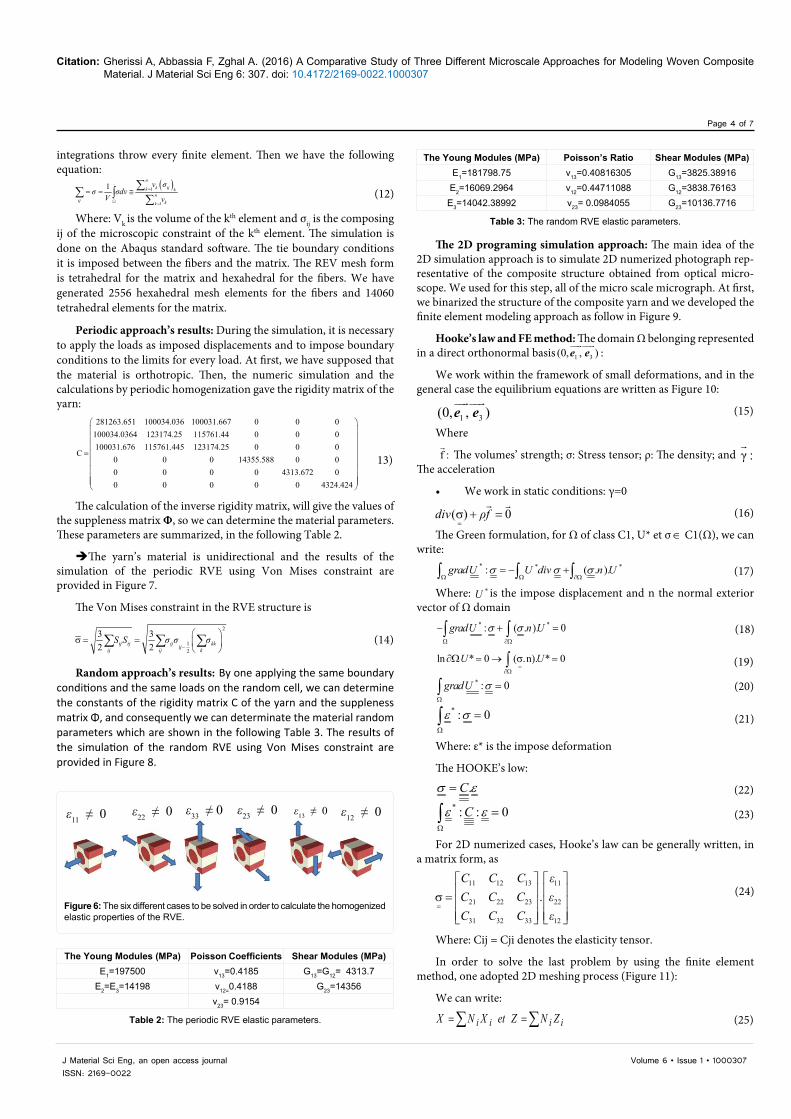
The micro scale constructive finite elements models: The adapted method consists in applying three simple traction loads following the three main axes (1, 2 and 3) and three simple shear loads in the directions 2-3, 1-2 and 2-3 (Figure 6). In order to apply this method, we should impose a displacement loading and put a specific boundary conditions for each load, this method has been adopted by several authors [10,14]. The calculation of ∑ij is approximated by the summation of all the volumetric elements of structure already calculated by elementariness

1.4

1.2

1

0.8

0.6

0.4

0.2

0

-0.210 20 30 40 50 60 70 80 90 100

Vf: Fibers volume fraction

Vf: The average volume fraction of fibers

α: Window size of the cell (µm)

vf minivf maxi

Figure 5: Variations in local volume fraction of fibres.


of 7


integrations throw every finite element. Then we have the following equation:

(12)

Where: Vk is the volume of the kth element and σij is the composing ij of the microscopic constraint of the kth element. The simulation is done on the Abaqus standard software. The tie boundary conditions it is imposed between the fibers and the matrix. The REV mesh form is tetrahedral for the matrix and hexahedral for the fibers. We have generated 2556 hexahedral mesh elements for the fibers and 14060 tetrahedral elements for the matrix.

Periodic approach’s results: During the simulation, it is necessary to apply the loads as imposed displacements and to impose boundary conditions to the limits for every load. At first, we have supposed that the material is orthotropic. Then, the numeric simulation and the calculations by periodic homogenization gave the rigidity matrix of the yarn:

281263.651 100034.036 100031.667 0 0 0100034.0364 123174.25 115761.44 0 0 0100031.676 115761.445 123174.25 0 0 0

C0 0 0 14355.588 0 00 0 0 0 4313.672 00 0 0 0 0 4324.424

=

13)

The calculation of the inverse rigidity matrix, will give the values of the suppleness matrix Φ, so we can determine the material parameters. These parameters are summarized, in the following Table 2.

The yarn’s material is unidirectional and the results of the simulation of the periodic RVE using Von Mises constraint are provided in Figure 7.

The Von Mises constraint in the RVE structure is

(14)

Random approach’s results: By one applying the same boundary conditions and the same loads on the random cell, we can determine the constants of the rigidity matrix C of the yarn and the suppleness matrix Φ, and consequently we can determinate the material random parameters which are shown in the following Table 3. The results of the simulation of the random RVE using Von Mises constraint are provided in Figure 8.

The 2D programing simulation approach: The main idea of the 2D simulation approach is to simulate 2D numerized photograph rep-resentative of the composite structure obtained from optical micro-scope. We used for this step, all of the micro scale micrograph. At first, we binarized the structure of the composite yarn and we developed the finite element modeling approach as follow in Figure 9.

Hooke’s law and FE method: The domain Ω belonging represented in a direct orthonormal basis 1 3(0, ),

e e :

We work within the framework of small deformations, and in the general case the equilibrium equations are written as Figure 10:

1 3(0, ),

e e (15)

Where

f :

The volumes’ strength; σ: Stress tensor; ρ: The density; and The acceleration

• We work in static conditions: γ=0

(16)

The Green formulation, for Ω of class C1, U* et σ ∈ C1(Ω), we can write:

* * *: ( . ).gradU U div n Uσ σ σΩ Ω ∂Ω

= − +∫ ∫ ∫ (17)

Where: *U is the impose displacement and n the normal exterior vector of Ω domain

* *: ( . ). 0gradU n Uσ σΩ ∂Ω

− + =∫ ∫ (18)

ln * 0 ( .n). * 0=

∂Ω

∂Ω = → σ =∫U U (19) * : 0gradU σ

Ω

=∫ (20)

* : 0ε σΩ

=∫ (21)

Where: ε* is the impose deformation

The HOOKE’s low:

.Cσ ε= (22)* : : 0Cε ε

Ω

=∫ (23)

For 2D numerized cases, Hooke’s law can be generally written, in a matrix form, as

(24)

Where: Cij = Cji denotes the elasticity tensor.

In order to solve the last problem by using the finite element method, one adopted 2D meshing process (Figure 11):

We can write:

i i i iX N X et Z N Z= =∑ ∑ (25)

ε11 ≠ 0 ε22 ≠ 0 ε33 ≠ 0 ε23 ≠ 0 ε13 ≠ 0 ε12 ≠ 0

Figure 6: The six different cases to be solved in order to calculate the homogenized elastic properties of the RVE.

The Young Modules (MPa) Poisson Coefficients Shear Modules (MPa)E1=197500 ν13=0.4185 G13=G12= 4313.7

E2=E3=14198 ν12=0.4188 G23=14356 ν23= 0.9154

Table 2: The periodic RVE elastic parameters.

The Young Modules (MPa) Poisson’s Ratio Shear Modules (MPa)E1=181798.75 ν13=0.40816305 G13=3825.38916

E2=16069.2964 ν12=0.44711088 G12=3838.76163E3=14042.38992 ν23= 0.0984055 G23=10136.7716

Table 3: The random RVE elastic parameters.


of 7


In the nodes, the corresponding functions of form will be:

( )( ) ( )( ) ( )( ) ( )( )1 2 3 41 1 1 11 1 ; 1 1 ; 1 1 ; 1 14 4 4 4

= − − = + − = + + = − +N N N Nξ η ξ η ξ η ξ η (26)

And the displacements:

i i i iu N u and w N w= =∑ ∑ (27)

∂∂∂∂

⋅

η∂∂

η∂∂

ξ∂∂

ξ∂∂

=

η∂∂ξ∂

∂

ZuXu

ZX

ZX

u

u

J

(28)

Where: J is the Jacobean matrix.

We can resolve (28) as:

* *11 12

∂ ∂ ∂= = +∂ ∂ ∂xxu u uJ Jx

εξ η

(29)

Where: J11 and J12 are J-1 coefficients.

;i ii i

u N w Nu wξ ξ η η

∂ ∂ ∂ ∂= =

∂ ∂ ∂ ∂∑ ∑ (30)

The εzz and γxz (2εxz ) deformation will be obtained by the same way,

therefore we can write:

1 .

2

u

xx wA Jzz

wxz

ε η

ε εξ

εη

∂ ∂ ∂ − = = ∂ ∂ ∂

(31)

It denotes that:

1 . . eA J B Uε − = (32)

Where [B]: the deformation-displacement matrix

Under these conditions, the elementary rigidity matrix will be written in the following form:

[ ]1 1

1 1[ ] [ ] [ ] [ ] [ ] [ ]T Tk B B dV B B J d dε ε ξ η

− −

= ⋅ ⋅ = ⋅ ⋅ ⋅∫ ∫ ∫ (33)

The numerical integration adopted for the equation (33), is the Gauss integration, which is written as following form:

1

11 =−

= Φ ==> ≈ Φ∑∫n

i ii

I d I Wξ (34)

Where: Wi are the Gauss weight and Φi are the Gauss points

We can calculate the global stiffness matrix:

Eq. (21), (32), (33) and (34) give that

ε11 ≠ 0 ε22 ≠ 0 ε23 ≠ 0

+4.207e+05+3.858e+05+3.509e+05+3.159e+05+2.810e+05+2.461e+05+2.112e+05+1.763e+05+1.414e+05+1.065e+05+7.163e+04+3.672e+04+1.819e+03

+1.236e+05+1.236e+05+1.137e+05+1.038e+05+9.390e+04+8.402e+04+7.413e+04+6.424e+04+5.435e+04+4.447e+04+3.458e+04+2.469e+04+1.480e+04

+1.909e+04+1.752e+04+1.596e+04+1.440e+04+1.284e+04+1.128e+04+9.713e+03+8.151e+03+6.589e+03+5.027e+03+3.465e+03+1.903e+03+3.407e+03

S, Mises(Avg: 75%)

S, Mises(Avg: 75%)

S, Mises(Avg: 75%)

Figure 7: Results of simulation of the RVE, Von Mises constraint in the different loads (plan y z).

ε11 ≠ 0

ε23 ≠ 0 ε13 ≠0 ε12 ≠0

ε23 ≠ 0 ε22 ≠ 0

+3,939e+05+3,614e+05+3,288e+05+2,962e+05+2,636e+05+2,310e+05+1,984e+05+1,658e+05+1,332e+05+1,006e+05+6,800e+04+3,540e+04+2,805e+03

+2,732e+04+2,507e+04+2,283e+04+2,058e+04+1,834e+04+1,610e+04+1,385e+04+1,161e+04+9,362e+03+1,117e+03+4,873e+03+3,629e+03+3,842e+03

+2,616e+04+2,400e+04+2,185e+04+2,970e+04+1,754e+04+1,539e+04+1,323e+04+1,108e+04+8,922e+03+6,767e+03+4,612e+03+3,458e+03+3,029e+02

+8,059e+04+7,390e+04+6,721e+04+6,052e+04+5,384e+04+4,715e+04+4,046e+04+3,377e+04+2,708e+04+2,039e+04+1,370e+04+7,012e+03+3,233e+02

+7,925e+04+7,269e+04+6,614e+04+5,958e+04+5,303e+04+4,648e+04+3,992e+04+3,337e+04+2,681e+04+2,026e+04+1,371e+04+7,153e+03+5,994e+02

+2,906e+04+2,670e+04+2,434e+04+2,198e+04+1,962e+04+1,726e+04+1,490e+04+1,254e+04+1,018e+04+7,817e+03+5,458e+03+3,098e+03+7,380e+02

S, Mises(Avg: 75%)

S, Mises(Avg: 75%)

S, Mises(Avg: 75%) S, Mises

(Avg: 75%)

S, Mises(Avg: 75%)

S, Mises(Avg: 75%)

Figure 8: The results of simulation of the RVE, Von Mises constraint in the different loads (plan y z).


of 7


* : . . . . . . . . .detpgpg

T T T T T TB Q A C A Q B w B Q A C A Q B Jε σΩ Ω

= =∑∫ ∫ (35)

Where: 1Q J−≡

The resolve of (35) it applied by imposing a displacements loading and putting a boundary conditions for each load see Figure 12.

The approach of finite element simulation in Matlab gives the following results:

222220 94570 094890 221480 0

0 0 4320

=

C (36)

Exx =181700 MPa Eyy=181100 MPaG=4320 MPa νxy=0.42

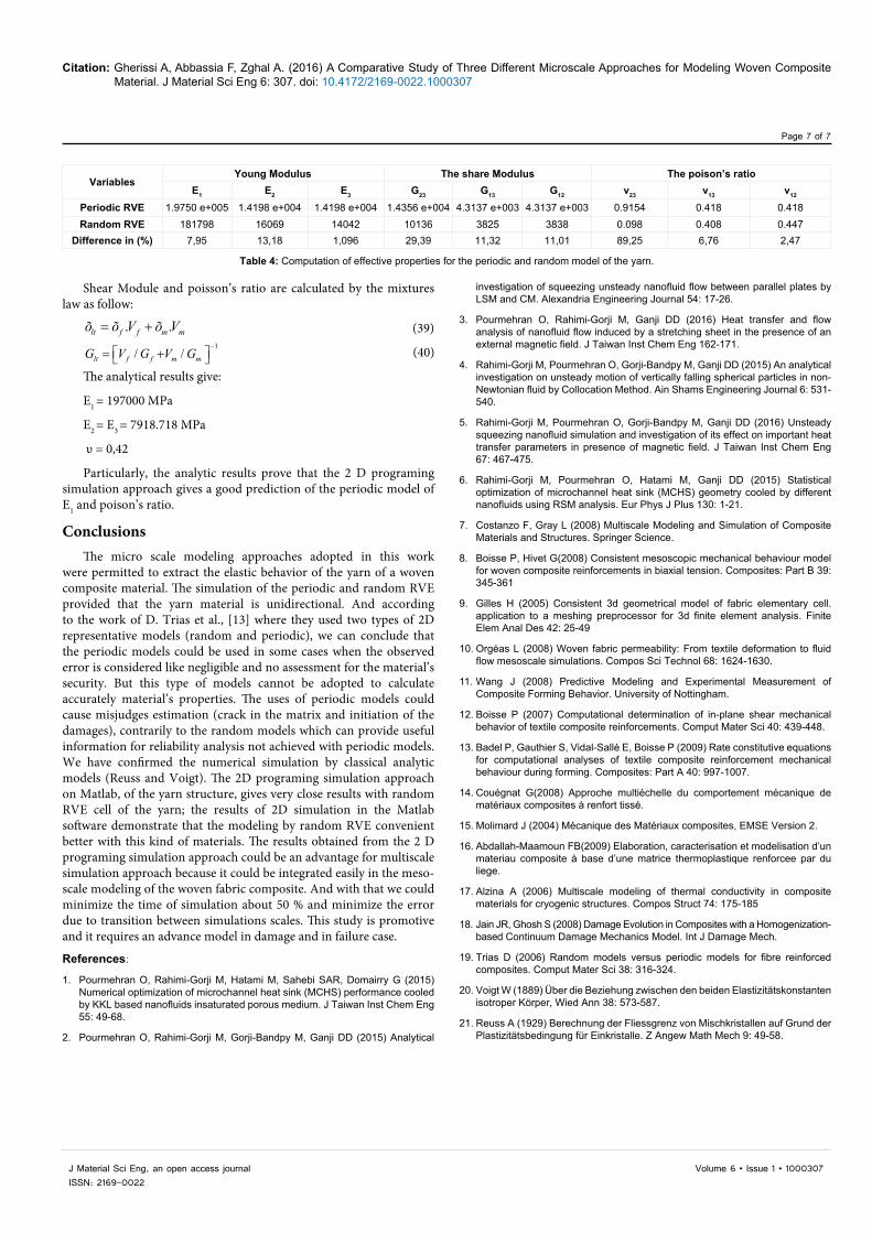
Comparison and discussion of the threetsimulation’s methods, 3D periodic, 3D random and 2D programing simulation approach: The results obtain for both 3D periodic and random model are reported in Table 4. The fluctuation in the Young modules and the Poisson’s ratio among the two models are as follow: the relative error for E2 reaches

13% and, for the Poisson’s coefficients ν12 and ν13 it is respectively 2.47% and 6.76%. These results converge with the 2D programing simulation approach for the simple traction following the (OY), this results was reported in the work of D.Trias et al., [19], where the Young modulus present a differentiation of 12% and 6% for the Poisson’s ratio.

The difference between the random and the periodic RVE in Shear Modulus G13 and G12 is roughly 11% and 29.39% for G23. Concerning the Poisson coefficient ν23 the relative error between the two models is around 89%.

For the periodic RVE, we could observe that the YOUNG modulus E2 and E3 have a regular behavior in the tow transverse directions. But for the random model, the difference between the two modulus E2 and E3 it is much remarkable. This difference is generally due to the arrangement of the fibers and the irregular of the distance inter-fibers. Also the variation of the value of E2 of 13% and the value of G23 of 29.39 % has been observed in the two cases random and periodic RVE. This deference is due to the closeness between fibers in the random RVE who will give a more resistance to the model.

The 2D programing simulation approach, of the yarn structure, gives very close results with random RVE cell of the yarn: (i.e.: E Random

RVE=181798 MPa and E2D=181700 MPa). The results of the distribution using Von Mises constraint in yarn it is show in Figures 5 and 6, they present a large difference between the two types of RVE. Indeed, the random model gives a more real response than the periodic model. The analytic values resulting from The Voigt model and the Reuss model [20,21] gives:

1/ /

− = + t f f m mE V E V E (37)

. .= +l f f m mE E V E V (38)

Binarization and filtration of themicrostructure of the yarn

Solving the homogenization’sproblem

Regular mesh and EF Simulation of the yarn

Extraction of the Cijcoefficients

Figure 9: The approach of 2D simulation approach of the yarn.

100

200

300

400

500

600

700

800

900

1000200 400 600 800 1000 1200

Ω

∂Ω

Figure 10: The micro structure of the yarn.

z, w

P4 P3

P1 P2

X, U

Figure 11: The 2D unit’s mesh.

ε11 ≠ 0 ε22 ≠ 0 ε12 ≠ 0

Figure 12: The three different cases to be solved for the homogenized elastic properties of the yarn.


of 7


Shear Module and poisson’s ratio are calculated by the mixtures law as follow:

. .= +lt f f m mõ õ V õ V (39)1

/ /−

= + lt f f m mG V G V G (40)

The analytical results give:

E1 = 197000 MPa

E2 = E3 = 7918.718 MPa

υ = 0,42

Particularly, the analytic results prove that the 2 D programing simulation approach gives a good prediction of the periodic model of E1 and poison’s ratio.

ConclusionsThe micro scale modeling approaches adopted in this work

were permitted to extract the elastic behavior of the yarn of a woven composite material. The simulation of the periodic and random RVE provided that the yarn material is unidirectional. And according to the work of D. Trias et al., [13] where they used two types of 2D representative models (random and periodic), we can conclude that the periodic models could be used in some cases when the observed error is considered like negligible and no assessment for the material’s security. But this type of models cannot be adopted to calculate accurately material’s properties. The uses of periodic models could cause misjudges estimation (crack in the matrix and initiation of the damages), contrarily to the random models which can provide useful information for reliability analysis not achieved with periodic models. We have confirmed the numerical simulation by classical analytic models (Reuss and Voigt). The 2D programing simulation approach on Matlab, of the yarn structure, gives very close results with random RVE cell of the yarn; the results of 2D simulation in the Matlab software demonstrate that the modeling by random RVE convenient better with this kind of materials. The results obtained from the 2 D programing simulation approach could be an advantage for multiscale simulation approach because it could be integrated easily in the meso-scale modeling of the woven fabric composite. And with that we could minimize the time of simulation about 50 % and minimize the error due to transition between simulations scales. This study is promotive and it requires an advance model in damage and in failure case.

References:

1. Pourmehran O, Rahimi-Gorji M, Hatami M, Sahebi SAR, Domairry G (2015) Numerical optimization of microchannel heat sink (MCHS) performance cooled by KKL based nanofluids insaturated porous medium. J Taiwan Inst Chem Eng 55: 49-68.

2. Pourmehran O, Rahimi-Gorji M, Gorji-Bandpy M, Ganji DD (2015) Analytical

investigation of squeezing unsteady nanofluid flow between parallel plates by LSM and CM. Alexandria Engineering Journal 54: 17-26.

3. Pourmehran O, Rahimi-Gorji M, Ganji DD (2016) Heat transfer and flow analysis of nanofluid flow induced by a stretching sheet in the presence of an external magnetic field. J Taiwan Inst Chem Eng 162-171.

4. Rahimi-Gorji M, Pourmehran O, Gorji-Bandpy M, Ganji DD (2015) An analytical investigation on unsteady motion of vertically falling spherical particles in non-Newtonian fluid by Collocation Method. Ain Shams Engineering Journal 6: 531-540.

5. Rahimi-Gorji M, Pourmehran O, Gorji-Bandpy M, Ganji DD (2016) Unsteady squeezing nanofluid simulation and investigation of its effect on important heat transfer parameters in presence of magnetic field. J Taiwan Inst Chem Eng 67: 467-475.

6. Rahimi-Gorji M, Pourmehran O, Hatami M, Ganji DD (2015) Statistical optimization of microchannel heat sink (MCHS) geometry cooled by different nanofluids using RSM analysis. Eur Phys J Plus 130: 1-21.

7. Costanzo F, Gray L (2008) Multiscale Modeling and Simulation of Composite Materials and Structures. Springer Science.

8. Boisse P, Hivet G(2008) Consistent mesoscopic mechanical behaviour model for woven composite reinforcements in biaxial tension. Composites: Part B 39: 345-361

9. Gilles H (2005) Consistent 3d geometrical model of fabric elementary cell. application to a meshing preprocessor for 3d finite element analysis. Finite Elem Anal Des 42: 25-49

10. Orgéas L (2008) Woven fabric permeability: From textile deformation to fluid flow mesoscale simulations. Compos Sci Technol 68: 1624-1630.

11. Wang J (2008) Predictive Modeling and Experimental Measurement of Composite Forming Behavior. University of Nottingham.

12. Boisse P (2007) Computational determination of in-plane shear mechanical behavior of textile composite reinforcements. Comput Mater Sci 40: 439-448.

13. Badel P, Gauthier S, Vidal-Sallé E, Boisse P (2009) Rate constitutive equations for computational analyses of textile composite reinforcement mechanical behaviour during forming. Composites: Part A 40: 997-1007.

14. Couégnat G(2008) Approche multiéchelle du comportement mécanique de matériaux composites à renfort tissé.

15. Molimard J (2004) Mécanique des Matériaux composites, EMSE Version 2.

16. Abdallah-Maamoun FB(2009) Elaboration, caracterisation et modelisation d’un materiau composite à base d’une matrice thermoplastique renforcee par du liege.

17. Alzina A (2006) Multiscale modeling of thermal conductivity in composite materials for cryogenic structures. Compos Struct 74: 175-185

18. Jain JR, Ghosh S (2008) Damage Evolution in Composites with a Homogenization-based Continuum Damage Mechanics Model. Int J Damage Mech.

19. Trias D (2006) Random models versus periodic models for fibre reinforced composites. Comput Mater Sci 38: 316-324.

20. Voigt W (1889) Über die Beziehung zwischen den beiden Elastizitätskonstanten isotroper Körper, Wied Ann 38: 573-587.

21. Reuss A (1929) Berechnung der Fliessgrenz von Mischkristallen auf Grund der Plastizitätsbedingung für Einkristalle. Z Angew Math Mech 9: 49-58.

VariablesYoung Modulus The share Modulus The poison’s ratio

E1 E2 E3 G23 G13 G12 ν23 ν13 ν12

Periodic RVE 1.9750 e+005 1.4198 e+004 1.4198 e+004 1.4356 e+004 4.3137 e+003 4.3137 e+003 0.9154 0.418 0.418 Random RVE 181798 16069 14042 10136 3825 3838 0.098 0.408 0.447

Difference in (%) 7,95 13,18 1,096 29,39 11,32 11,01 89,25 6,76 2,47

Table 4: Computation of effective properties for the periodic and random model of the yarn.

http://dx.doi.org/10.1016%2Fj.jtice.2015.04.016




http://dx.doi.org/10.1016%2Fj.aej.2014.11.002



http://dx.doi.org/10.1016%2Fj.asej.2014.10.016




http://dx.doi.org/10.1140/epjp/i2015-15022-8



http://dx.doi.org/10.1016%2Fj.compositesb.2007.01.011



https://doi.org/10.1016/j.finel.2005.05.001



http://dx.doi.org/10.1016%2Fj.compscitech.2008.02.027

http://dx.doi.org/10.1016%2Fj.compscitech.2008.02.027

http://eprints.nottingham.ac.uk/10602/

http://eprints.nottingham.ac.uk/10602/

http://dx.doi.org/10.1016%2Fj.commatsci.2007.01.022


http://dx.doi.org/10.1016/j.compositesa.2008.04.015



https://tel.archives-ouvertes.fr/tel-00403885/

https://tel.archives-ouvertes.fr/tel-00403885/

http://dx.doi.org/10.1016%2Fj.compstruct.2005.04.002

http://dx.doi.org/10.1016%2Fj.compstruct.2005.04.002



http://dx.doi.org/10.1002/zamm.19290090104

http://dx.doi.org/10.1002/zamm.19290090104

journal of material sciences engineering

Documents