journal of hydraulic research experimental and numerical

PLEASE SCROLL DOWN FOR ARTICLE

This article was downloaded by: [Dewals, Benjamin]On: 1 July 2010Access details: Access Details: [subscription number 921481097]Publisher Taylor & FrancisInforma Ltd Registered in England and Wales Registered Number: 1072954 Registered office: Mortimer House, 37-41 Mortimer Street, London W1T 3JH, UK

Journal of Hydraulic ResearchPublication details, including instructions for authors and subscription information:http://www.informaworld.com/smpp/title~content=t916282780

Experimental and numerical investigations of dike-break induced flowsSebastian Rogera; Benjamin J. Dewalsb; Sébastien Erpicumc; Dirk Schwanenbergd; Holger Schüttrumpfe;Jürgen Köngeterf; Michel Pirottonc

a Institute of Hydraulic Engineering and Water Resources Management (IWW), RWTH AachenUniversity, Hydraulic Laboratory, Aachen, Germany b Unit of Hydrology, Applied Hydrodynamicsand Hydraulic Constructions (HACH), Department ArGEnCo, University of Liege (ULg) and Fund forScientific Research F.R.S.-FNRS, Belgium c HACH, Department ArGEnCo, University of Liege (ULg),Belgium d Deltares, Operational Water Management, Delft, NL e IWW, RWTH Aachen University,Germany f IWW, RWTH Aachen University,, Germany

Online publication date: 26 April 2010

To cite this Article Roger, Sebastian , Dewals, Benjamin J. , Erpicum, Sébastien , Schwanenberg, Dirk , Schüttrumpf,Holger , Köngeter, Jürgen and Pirotton, Michel(2009) 'Experimental and numerical investigations of dike-break inducedflows', Journal of Hydraulic Research, 47: 3, 349 — 359To link to this Article: DOI: 10.1080/00221686.2009.9522006URL: http://dx.doi.org/10.1080/00221686.2009.9522006

Full terms and conditions of use: http://www.informaworld.com/terms-and-conditions-of-access.pdf

This article may be used for research, teaching and private study purposes. Any substantial orsystematic reproduction, re-distribution, re-selling, loan or sub-licensing, systematic supply ordistribution in any form to anyone is expressly forbidden.

The publisher does not give any warranty express or implied or make any representation that the contentswill be complete or accurate or up to date. The accuracy of any instructions, formulae and drug dosesshould be independently verified with primary sources. The publisher shall not be liable for any loss,actions, claims, proceedings, demand or costs or damages whatsoever or howsoever caused arising directlyor indirectly in connection with or arising out of the use of this material.

http://www.informaworld.com/smpp/title~content=t916282780

http://dx.doi.org/10.1080/00221686.2009.9522006

http://www.informaworld.com/terms-and-conditions-of-access.pdf

Journal of Hydraulic Research Vol. 47, No. 3 (2009), pp. 349–359

doi:10.3826/jhr.2009.3472

© 2009 International Association of Hydraulic Engineering and Research

Experimental and numerical investigations of dike-break induced flows

Investigations expérimentales et numériques sur les écoulements induitspar les ruptures de diguesSEBASTIAN ROGER, Institute of Hydraulic Engineering and Water Resources Management (IWW), RWTH Aachen University,Hydraulic Laboratory, Kreuzherrenstr. 7, 52056 Aachen, Germany. Tel.: +(49) 241 80 93938; fax: +(49) 241 80 92275;E-mail: [email protected] (author for correspondence)

BENJAMIN J. DEWALS, (IAHR Member), Unit of Hydrology, Applied Hydrodynamics and Hydraulic Constructions (HACH),Department ArGEnCo, University of Liege (ULg) and Fund for Scientific Research F.R.S.-FNRS, Belgium.E-mail: [email protected]

SÉBASTIEN ERPICUM, (IAHR Member), HACH, Department ArGEnCo, University of Liege (ULg), Belgium.E-mail: [email protected]

DIRK SCHWANENBERG, (IAHR Member), Deltares, Operational Water Management, Delft, NL.E-mail: [email protected]

HOLGER SCHÜTTRUMPF, (IAHR Member), IWW, RWTH Aachen University, Germany. E-mail:[email protected]

JÜRGEN KÖNGETER, (IAHR Member), IWW, RWTH Aachen University, Germany. E-mail: [email protected]

MICHEL PIROTTON, HACH, Department ArGEnCo, University of Liege (ULg), Belgium. E-mail: [email protected]

ABSTRACTExperimental model data are compared with numerical computations of dike-break induced flows, focusing on the final steady state. An idealized scalemodel was designed reproducing the specific boundary conditions of dike breaks. Discharges, water level, and depth profiles of horizontal velocitieswere recorded and validated by numerical modeling. The latter was performed by two different models solving the two-dimensional depth-averagedshallow water equations, namely a total variation diminishing Runge-Kutta discontinuous Galerkin finite element method, and a finite volume schemeinvolving a flux vector splitting approach. The results confirmed convergence and general applicability of both methods for dike-break problems. Asregards their accuracy, the basic flow pattern was satisfactorily reproduced yet with differences compared to the measurements. Hence, additionalsimulations by the finite volume model were performed considering various turbulence closures, wall-roughnesses as well as nonuniform Boussinesqcoefficients.

RÉSUMÉDes données de modèles expérimentaux sont comparées aux calculs numériques des écoulements induits par les ruptures de digues, en se concentrantsur l’état d’équilibre final. Un modèle réduit idéalisé a été conçu pour reproduire les conditions aux limites spécifiques des ruptures de digues. Lesdébits, le niveau d’eau, et les profils verticaux des vitesses horizontales ont été enregistrés et validés par modélisation numérique. Le dernier a étéréalisé par deux modèles différents résolvant les équations bidimensionnelles en eau peu profonde moyennées sur la hauteur, à savoir une méthodeTVD (total variation diminishing) de Runge-Kutta Galerkin discontinue en éléments finis, et un schéma en volumes finis comportant un splitting duvecteur flux. Les résultats ont confirmé la convergence et l’applicabilité générale des deux méthodes pour les problèmes de rupture de digues. En cequi concerne leur exactitude, la configuration de base de l’écoulement a été reproduite d’une manière satisfaisante avec cependant des différencespar rapport aux mesures. C’est pourquoi, des simulations additionnelles ont été effectuées avec un modèle en volumes finis en considérant diversesfermetures de la turbulence, et rugosités de paroi, ainsi que des coefficients de Boussinesq non-uniformes.

Keywords: Boussinesq coefficients, discontinuous Galerkin, dike break, shallow water

1 Introduction

1.1 Motivation

Dikes or (mobile) walls are essential parts of flood protectionconceptions along river banks to protect densely populated areas

Revision received January 13, 2009/Open for discussion until December 31, 2009.

349

from flooding. Massive flood events and recurring dike failures

indicate that inland flood protection systems may be vulnera-

ble. The assessment of this risk involves the identification of

inundated areas as well as flow depths and velocities of the ini-

tiated wave. In this context, the discharge through the breach of

Downloaded By: [Dewals, Benjamin] At: 10:48 1 July 2010

350 S. Roger et al. Journal of Hydraulic Research Vol. 47, No. 3 (2009)

a collapsed dike section significantly affects the final water leveland its rising speed in the floodplain.

The static impact for a slow increase of the water level in afloodplain basically depends on the total water volume enteringthe floodplain over a long period, while during the first transientphase of a dike break, flow velocities and water depths within theflood wave induce dynamic damages nearby the breach. Com-pared to the duration of the whole event this period is often shortbut equally dangerous for people and property.

Beside the damage calculation in a risk assessment proce-dure, the results of flood wave computations are used to managethe residual risk. The definition of evacuation zones, the coordi-nation of civil protection and emergency measures as well asthe land use planning are important for risk mitigation. Thesimulation of various scenarios may provide authorities withvaluable information in terms of flood arrival time and mainflow directions. Additional applications include the design andrisk analysis of mobile flood protection systems in combinationwith the determination of safety areas. Insurance companies alsohave an interest in modifying their computational approaches asregards damage categories. Moreover, there are European legalattempts to identify and to illustrate areas with a significant floodrisk.

1.2 Phenomenon and procedure

The wide knowledge concerning dam-break waves (CADAM2000, IMPACT 2005) cannot directly be transferred to dike-breakinduced flows. The latter are influenced by the momentum com-ponent parallel to the protection structure causing asymmetricflood wave propagation. Moreover, unlike reservoirs at rest, ariver bed will not be empty, but the persisting flood dischargeleads to a fixed water level in the breach as the final steadystate is approached resulting in a partition of the inflow into thedownstream and the breach discharges (Fig. 1). This state has tobe considered when focusing the long-term inundation and theresulting static impact in the entire floodplain. There is a lack ofknowledge as regards these types of flood waves. The existingmeasured data are not sufficient due to the unpredictability andthe danger of such events.

There exist only few investigations considering the propaga-tion of a wave into an area, such as Fraccarollo and Toro (1995)or Kulisch (2003), relating to dam-break flows, however. Aureliand Mignosa (2002, 2004) only considered the presence of apermanent river discharge.

Circumventing the expense of a full-sized prototype, a bench-scale model was used to provide experimental data, which wererecorded with sophisticated measurement techniques to exploreflow effects and to validate numerical models. Physical andnumerical models were combined in a hybrid approach. On theone hand, the accuracy of numerical forecasts was quantifiedby measurements. On the other hand, numerical simulationscomplement the model tests by calculating scenarios of differ-ent configurations, geometries and boundary conditions. Hence,this combination enables selective improvements in numericalmethods and more reliable forecasts for long-term and large-scale

Figure 1 (a) Dam-break versus (b) dike-break induced flow

applications. The experimental and numerical parts of thisresearch are detailed in Section 2. The mathematical modelis presented in Section 3, while its numerical implementationin two distinct simulation models follows in Section 4. Sec-tion 5 highlights the ability of both models to represent the maincharacteristics of dike-break induced flows under four differ-ent hydraulic conditions. Next, the measurements are comparedwith additional results obtained with the finite volume model,taking into consideration different turbulence closures, wallroughness and Boussinesq coefficients. Finally, conclusions aredrawn.

2 Scale model tests

2.1 Apparatus and idealized experimental set-up

The model shown in Fig. 2 was designed taking into account thespecial boundary conditions of a dike-break induced flow closeto the breach section (Briechle et al. 2004, Briechle 2006). Itconsists of a 1 m wide horizontal channel with a pneumaticallydriven gate at one bank and a 3.5 × 4.0 m2 adjacent propagationarea made of glass. A complete gate opening takes less than 0.3 s,representing the worst case scenario of a sudden and total dikefailure. Moreover, the opening mechanism is a combination ofpull and rotation to minimize effects on the free water column asthe wave is initiated.

In contrast to flumes, the water propagates radially and falls offthe glass plate freely at three sides. The bottom of the propagationarea is made of glass to enable laser measurements from belowthe plate. Initial channel water levels were 0.3 to 0.5 m, channeldischarges 0.1 to 0.3 m3/s, and breach widths between 0.3 and0.7 m.


Journal of Hydraulic Research Vol. 47, No. 3 (2009) Experimental and numerical investigations of dike-break induced flows 351

Figure 2 Scale model set-up

2.2 Measuring techniques

As regards the boundary conditions, the inflow was controlledvia an ultrasonic flow-measuring device. A weir at the chan-nel end was calibrated for different crest heights to controlthe initial water depth. The steady-state breach discharge QB

was indirectly calculated as the difference between the modelinflow and the weir overflow Qw. Due to strong spatial vari-ations of the initiated wave and air entrainment, an advancednonintrusive measuring techniques was necessary, providinghigh frequency and stability toward highly unsteady waterlevels.

Thus, water depths were recorded by ultrasonic sensors with25 Hz frequency all over the propagation area with grid lengthsof �x = �y = 0.2 m, and a refined grid of 0.1 m close to thebreach zone. Within the channel, the detection was performed atvarious cross-sections, again using a higher resolution up to 0.5 mfrom the breach section. The sensors were mounted on movablecross-beams enabling measurements at various locations. Despitethe steep wave front at some locations, errors were usually lessthan ±2 mm because the adopted sensors have an operatingrange of 0.35 m for the small detection zone considered with0.18 mm resolution. Detections at each grid point consisted of500 single values which were statistically evaluated, and the testreproducibility was also checked. Up to eight sensors were usedsimultaneously. Mean depth-averaged velocity profiles u(z), v(z)were sampled using a conventional 1D Laser-DopplerAnemome-ter (LDA), mounted on an automatic traversing unit beneath theglass plate. At the three cross-sections y = 0.25, 0.30, 0.35 mnear the breach the depth-averaged velocity components weremeasured using a denser grid of �x = 0.05 m, �z = 0.01 mwithin the wave.

3 Mathematical model

3.1 Governing equations

Both models are based on the 2D depth-averaged equations ofmass and momentum conservation, referred to as the Shallow-Water Equations (SWE). The basic assumption states that veloc-ities normal to the main flow directions remain small. As aconsequence the pressure field is hydrostatic, which may limitthe applicability of the SWE. Their conservative form can bewritten as follows, using vector notation

∂ts + ∂xf + ∂yg + ∂xfd + ∂ygd = So − Sf , (1)

s =

h

hu

hv

, So =

0∂xzb

∂yzb

, Sf =

0τbx/ρ

τby/ρ

, (2)

f =

hu

ρxxhu2 + 12gh2

ρxyhuv

, fd = −h

ρ

0σx

τxy

, (3)

g =

hv

ρxyhuv

ρyyhv2 + 12gh2

, gd = −h

ρ

0τxy

σy

, (4)

where s is the vector of conservative unknowns, t is the time,f, g are the advective and pressure fluxes in directions x andy, fd , gd are the diffusive fluxes, So is the bottom slope, Sf

is the friction slope, h is the flow depth, u, v are the depth-averaged velocity components in x- and y-directions, zb is thebottom elevation, g is the gravitational acceleration, ρ is the waterdensity, τbx, τby are the bottom shear stresses, and σx, σy, τxy are



the turbulent stresses. The Boussinesq coefficients ρxx, ρyy, ρxy

account for uneven distributed local flow velocities u, v overthe flow depth with angle brackets representing depth-averaging,namely

ρxx = 〈u2〉/u2 ≥ 1 and ρyy = 〈v2〉/v2 ≥ 1,

ρxy = 〈uv〉/uv, ρ2xy ≤ ρxxρyy.

(5)

3.2 Closure relations

The bottom friction is conventionally modeled using an empiricallaw, such as the Manning formula. The models enable the defini-tion of a spatially distributed roughness coefficient. Besides, thefinite volume model provides the additional possibility to repro-duce friction along the side walls by means of a process-orientedformulation (Dewals 2006, Dewals et al. 2008) as

τbx

ρgh= u

√

u2 + v2n2

b

h4/3+

Nx∑kx=1

4

3

ukxn2w

h1/3kx

�y

,

τby

ρgh= v

√

u2 + v2n2

b

h4/3+

Ny∑ky=1

4

3

vky n3/2w

h1/3ky

�x

,

(6)

where the Manning coefficients nb and nw (s/m1/3) characterizebottom and side-wall roughnesses, respectively. Nx and Ny des-ignate the number of edges of the finite volume cell which are incontact with the side-wall.

The turbulent stresses are expressed following the Boussinesqapproximation (ASCE 1988, Rodi 1984)

σx = 2ρ(ν + νT )∂xu, σy = 2ρ(ν + νT )∂yv,

τxy = τyx = (ν + νT )ρ(∂yu + ∂xv), (ν � νT ),(7)

where νt is the depth-averaged turbulent eddy viscosity, and ν isthe molecular kinematic viscosity.

4 Computational models

The mathematical model described above was implementedwithin two different computational models of which Table 1details the main characteristics.

Table 1 Comparison of FE model versus FV model

FE model FV model

Model name DGFlow WOLF 2DModel type Finite Element Finite VolumeSpace discretization Discontinuous Flux Vector

Galerkin (DG) Splitting (FVS)Time integration TVD Runge-Kutta Runge-KuttaGrid Triangular CartesianTurbulence closure None Algebraic/k-εWall roughness None Accounted forBoussinesq coefficients Set to unity Distributed values

4.1 Finite element model (FE model): DGFlow

DGFlow is based on the Runge-Kutta discontinuous Galerkin(RKDG) method for hyperbolic equation systems and the localdiscontinuous Galerkin method for advection-dominated flows(Cockburn 1999, Cockburn et al. 2000). The leadoff imple-mentation of the RKDG method to the SWE was presented bySchwanenberg and Köngeter (2000). Schwanenberg and Harms(2002, 2004) gave first applications to dam-break flows anddeveloped the Total Variation Diminishing (TVD) RKDG finiteelement method, which is frequently applied at IWW, RWTHAachen University. The scheme can be divided into three mainsteps:

— DG space discretization with a polynomial degree k decou-ples the partial differential equation into a set of ordinarydifferential equations,

— Ordinary differential equations are integrated in time by a(k + 1)-order TVD RK method, and

— Slope limiter is applied on every intermediate time step.

The scheme is well suited to handle complicated geometries andrequires only a simple treatment of boundary conditions andsource terms to obtain high-order accuracy and sharp representa-tion of shocks. By using orthogonal shape functions the resultingmass matrix becomes diagonal. Together with the explicit timeintegration, RKDG is computationally as efficient for transcriti-cal, convection-dominated shallow water flows on unstructured2D grids as comparable state-of-the-art finite volume schemes(Shu 2003). Furthermore, the computation of a numerical flux atthe intercell boundaries introduces up-winding into the schemewhile keeping the Galerkin test function inside the element.A slope limiter guarantees stability at shock zones by intro-ducing a selective amount of dissipation for pure hyperbolicproblems.

A detailed presentation as regards the space and time dis-cretization, the approximation of the numerical flux for the DGmethod and the description of the slope limiter were presented bySchwanenberg (2003) and Schwanenberg and Harms (2004). Asyet, the current model version has mainly been applied to dam-break flows. Therefore, viscous effects are neglected comparedto the convective transport in the main direction. Moreover, themomentum correction coefficients are set to unity, i.e.

fd = gd = 0 and ρxx = ρyy = ρxy = 1. (8)

The effects of these simplifications as regards dike-break inducedflows are analyzed with the FV model described below.

4.2 Finite volume model (FV model): WOLF 2D

The depth-averaged flow model WOLF 2D was developed at theUniversity of Liege for about a decade. It includes a mesh gen-erator and deals with multi-block Cartesian grids. This featureincreases the size of possible simulation domains and enableslocal mesh refinements close to interesting areas, while preserv-ing lower computational cost required by Cartesian comparedto unstructured grids. A grid adaptation technique restricts the



simulation domain to the wet cells. The space discretization ofthe divergence form of Eq. (1) is performed by means of a FiniteVolume scheme (FV). Variable reconstruction at cells interfacesis either constant or linear, combined with a slope limiter, leadingin the latter case to second-order space accuracy.

Appropriate flux computation has always been a challengingissue in finite volume schemes. Herein, the fluxes f and g werecomputed by a Flux Vector Splitting (FVS) method developedby HACH, University of Liege. Following this FVS, the up-winding direction of each flux term f and g is simply dictatedby the sign of the flow velocity reconstructed at the cell inter-faces. A “von Neumann” stability analysis has demonstrated thatFVS then leads to a stable spatial discretization of the gradientsf and g in Eq. (1) (Dewals 2006). Besides requiring low compu-tational cost, this FVS offers the advantages of being completelyFroude-independent and of facilitating a satisfactory adequacywith the discretization of the bottom slope term. This FVS hasalready proven its validity and efficiency for numerous applica-tions (Dewals 2006, Dewals et al. 2006a, 2006b, 2008, Erpicum2006, Erpicum et al. 2007). Due to their diffusive nature, thefluxes fd and gd are legitimately evaluated by means of a centeredscheme.

Since the model is applied to compute steady-state solutions,the time integration is performed by means of a 3-step first-orderaccurate Runge-Kutta algorithm, providing adequate dissipationin time. For stability reasons, the time step was constrained bythe Courant-Friedrichs-Lewy (CFL) condition based on gravitywaves. A semi-implicit treatment of the bottom friction term inEq. (6) was used, without requiring additional computationalcost.

Besides, wetting and drying of cells is handled free of vol-ume and momentum conservation error by means of an iterativeresolution of the continuity equation at each time step (Erpicum2006). A four-step procedure was followed at each temporal stepintegration:

(1) Continuity equation is evaluated,(2) Algorithm detects cells with a negative flow depth to reduce

the outflow unit discharge such that the computed water depthin these cells is strictly equal to zero,

(3) Since these flux corrections may induce the drying in cascadeof neighboring cells, steps 1 to 3 are repeated iteratively, and

(4) Momentum equations are computed based on the correctedunit discharge values.

In most practical applications, no more than two iterations arenecessary, keeping thus the computation cost limited.

Several turbulence models are implemented in the FV model,starting from simple algebraic expressions of turbulent viscosity,to a depth-integrated model involving additional partial differen-tial equations. Two different approaches were compared herein(see Subsection 5.5). First, a simple algebraic turbulence clo-sure was adopted, assuming that turbulence is bed-dominated,for which the turbulent kinematic viscosity may be expressedwith α ≈ 0.5 (Fisher et al. 1979) as

νT = αhu∗, (9)

and friction velocity u∗ defined as (Ghamry and Steffler 2002)

u2∗ =

√τ2bx + τ2

by

/ρ. (10)

Second, a depth-averaged k-ε model with two different length-scales accounting for vertical and horizontal turbulence mixingwas applied, as developed by Erpicum (2006).

4.3 Boundary conditions

In both computational models, the value of the specific dischargecan be prescribed as an inflow boundary condition. Besides, thetransverse specific inflow discharge is usually set to zero. Theoutflow boundary condition may be a water surface elevation, aFroude number or no specific condition if the outflow is super-critical. At solid walls, the component of the specific dischargenormal to it was set to zero.

In the FV model, to evaluate the diffusive terms, the gradientsof the unknowns in the direction parallel to the boundary wereset to zero for simplicity, while the gradients of the variablesin the direction normal to the boundary were properly evaluatedby finite differences between the boundary value and the centervalue of the adjacent cell (Erpicum 2006). Regarding turbulencevariables, the law of the wall was used to compute shear velocityon solid walls to determine the corresponding depth-averaged tur-bulent kinetic energy and its dissipation rate (Rodi 1984, Younusand Chaudhry 1994). At inlets, the turbulent kinetic energy andits dissipation rate were also prescribed (Choi and Garcia 2002,Ferziger and Peric 2002).

5 Numerical tests and results

5.1 Computational procedure and grid

Although the present analysis explicitly focused on steady-stateconditions, both computational models were run starting from aninitial condition corresponding to steady channel flow. The wholetransient propagation and development of the dike break wave hasbeen simulated until the final steady solution was achieved.

The Cartesian grid used in the FV model involved almost60,000 cells 0.02 m by 0.02 m. In contrast, the FE model sim-ulations based upon about 23,000 triangular cells and 12,000discrete nodes, with an average element edge length of 0.05 m.Nearby the breach, local grid refinement was used resulting in0.03 m edges. After describing the various tested configurationsas well as the corresponding boundary conditions (5.2), the fol-lowing subsections successively include base simulations, effectsof second order space discretization, turbulence modeling, bedand wall friction as well as Boussinesq coefficients.

5.2 Test configurations

Four different initial hydraulic configurations were considered,depending on the inflow discharge and the initial channel flowdepth. Before each model run, a steady flow was established inthe channel with the corresponding initial flow depth. Preferably



Table 2 Definition of test configurations in numerical simulations forbreach width of 0.70 m

Test ID Inflow discharge Initial depth Crest height[m3/s] [m] [m]

Q300-h50 0.300 0.50 0.241Q300-h40 0.300 0.40 0.152Q200-h50 0.200 0.50 0.297Q200-h40 0.200 0.40 0.202

high values of the flow depth were adopted to result in high valuesof downstream and breach discharges after the flow split, to obtainmoderate velocities in the channel. Table 2 defines each of theseconfigurations. At the channel inlet (Fig. 2), the unit dischargewas prescribed as an upstream boundary condition. At the edgesof the propagation area (glass plate) no boundary condition wasneeded for supercritical outflow.

Calibrated weir formulas for various crest heights (Table 2)were implemented in both codes as possible downstream bound-ary conditions. Thus, the dynamics of the weir dischargedepending on the actual channel water level could be modeled.The resulting backwater effects and flow resistances interact withthe flow split into breach discharge and downstream channel dis-charge. The rating curve of each of those weirs was determinedexperimentally using a variable discharge coefficient as

Qw = 2

3µb

√2g(h − hw)3/2 = 2

3µ

√2gh

3/20 , (11)

where Qw is the weir discharge, µ is the discharge coefficient,b is the crest width of 1.0 m, h is the upstream water depth, hw

is the crest height, and h0 = h − hw as overflow depth. Thedischarge coefficient measured experimentally was expressed asa cubic polynomial of h0 (Table 3)

µ = a3h30 + a2h

20 + a1h0 + a0. (12)

5.3 Base simulations: Second order accurate spacediscretization with FE model and FV model

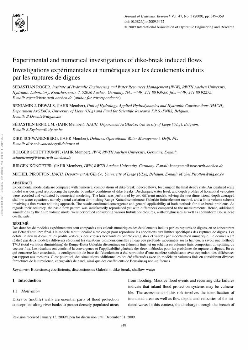
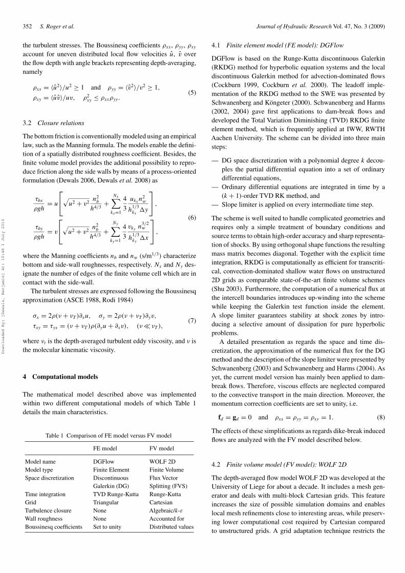
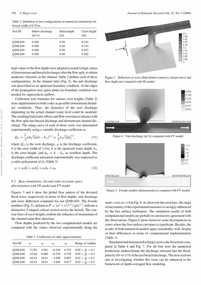
Figures 3 and 4 show the global flow pattern of the deviatedflood wave, respectively in terms of flow depths, unit dischargeand wave deflection computed for test Q300-h50. The Froudenumbers (Fig. 5), defined as F = (u2 +v2)1/2/(gh)1/2, indicate adistinctive S-shaped critical section across the breach. The con-tour lines of wave heights confirm the influence of momentum ofthe channel main flow direction.

Flow depths predicted by the two computational models arecompared with the values observed experimentally along the

Table 3 Coefficients of cubic approximations

Test ID a3 a2 a1 a0 Range of validity

Q300-h50 –7.291 4.561 –0.554 0.752 0.05 < Q < 0.3Q300-h40 –10.84 6.009 –0.359 0.738 0.05 < Q < 0.3Q200-h50 –62.63 26.61 –3.508 0.887 0.03 < Q < 0.2Q200-h40 –65.62 29.01 –3.665 0.877 0.03 < Q < 0.2

Figure 3 Deflection of wave (dash-dotted contours), stream traces andflow depth [m] computed with FE model

Figure 4 Unit discharge [m2/s] computed with FV model

Figure 5 Froude number [dimensionless] computed with FV model

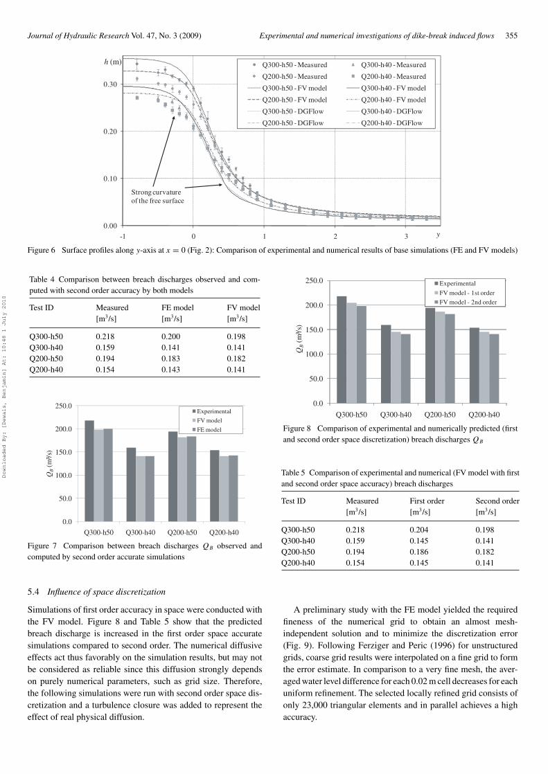
main y-axis at x = 0 in Fig. 6. As shown by the error bars, the rangeof uncertainty of the experimental measures is strongly influencedby the free surface inclination. The simulation results of bothcomputational models are globally in satisfactory agreement withthe observations. Figure 6 shows however some discrepancies inzones where the free surface curvature is significant. Besides, theresults of both numerical models agree remarkably well, despiteof their differences in terms of computational implementation(Table 1).

Simulated and measured discharges across the breach are com-pared in Table 4 and Fig. 7. For all four tests the numericalpredictions underestimate the discharge released into the flood-plain by 6% to 11% of the test breach discharge. The next sectionsaim at investigating whether this issue can be enhanced in theframework of depth-averaged flow modeling.



0.00

0.10

0.20

0.30

-1 0 1 2 3

h (m)

y

Q300-h50 - Measured Q300-h40 - Measured

Q200-h50 - Measured Q200-h40 - Measured

Q300-h50 - FV model Q300-h40 - FV model

Q200-h50 - FV model Q200-h40 - FV model

Q300-h50 - DGFlow Q300-h40 - DGFlow

Q200-h50 - DGFlow Q200-h40 - DGFlow

Strong curvatureof the free surface

Figure 6 Surface profiles along y-axis at x = 0 (Fig. 2): Comparison of experimental and numerical results of base simulations (FE and FV models)

Table 4 Comparison between breach discharges observed and com-puted with second order accuracy by both models

Test ID Measured FE model FV model[m3/s] [m3/s] [m3/s]

Q300-h50 0.218 0.200 0.198Q300-h40 0.159 0.141 0.141Q200-h50 0.194 0.183 0.182Q200-h40 0.154 0.143 0.141

0.0

50.0

100.0

150.0

200.0

250.0

Q300-h50 Q300-h40 Q200-h50 Q200-h40

QB

(m³/

s)

Experimental

FV model

FE model

Figure 7 Comparison between breach discharges QB observed andcomputed by second order accurate simulations

5.4 Influence of space discretization

Simulations of first order accuracy in space were conducted withthe FV model. Figure 8 and Table 5 show that the predictedbreach discharge is increased in the first order space accuratesimulations compared to second order. The numerical diffusiveeffects act thus favorably on the simulation results, but may notbe considered as reliable since this diffusion strongly dependson purely numerical parameters, such as grid size. Therefore,the following simulations were run with second order space dis-cretization and a turbulence closure was added to represent theeffect of real physical diffusion.

QB

(m³/

s)

0.0

50.0

100.0

150.0

200.0

250.0

Q300-h50 Q300-h40 Q200-h50 Q200-h40

Experimental

FV model - 1st order

FV model - 2nd order

Figure 8 Comparison of experimental and numerically predicted (firstand second order space discretization) breach discharges QB

Table 5 Comparison of experimental and numerical (FV model with firstand second order space accuracy) breach discharges

Test ID Measured First order Second order[m3/s] [m3/s] [m3/s]

Q300-h50 0.218 0.204 0.198Q300-h40 0.159 0.145 0.141Q200-h50 0.194 0.186 0.182Q200-h40 0.154 0.145 0.141

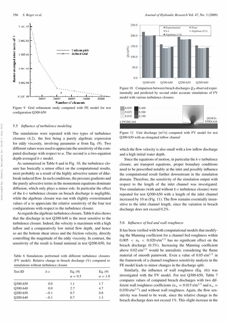
A preliminary study with the FE model yielded the requiredfineness of the numerical grid to obtain an almost mesh-independent solution and to minimize the discretization error(Fig. 9). Following Ferziger and Peric (1996) for unstructuredgrids, coarse grid results were interpolated on a fine grid to formthe error estimate. In comparison to a very fine mesh, the aver-aged water level difference for each 0.02 m cell decreases for eachuniform refinement. The selected locally refined grid consists ofonly 23,000 triangular elements and in parallel achieves a highaccuracy.



Figure 9 Grid refinement study computed with FE model for testconfiguration Q300-h50

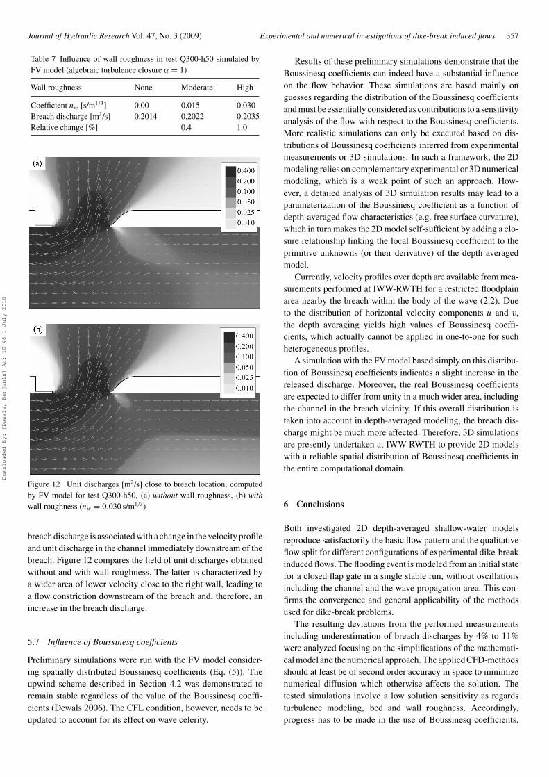
5.5 Influence of turbulence modeling

The simulations were repeated with two types of turbulenceclosures (4.2), the first being a purely algebraic expressionfor eddy viscosity, involving parameter α from Eq. (9). Twodifferent values were used to appreciate the sensitivity of the com-puted discharge with respect to α. The second is a two-equationdepth-averaged k-ε model.

As summarized in Table 6 and in Fig. 10, the turbulence clo-sure has basically a minor effect on the computational results,most probably as a result of the highly advective nature of dike-break induced flow. In such conditions, the pressure gradients andthe purely advective terms in the momentum equations dominatediffusion, which only plays a minor role. In particular the effectof the k-ε turbulence closure on breach discharge is negligible,while the algebraic closure was run with slightly overestimatedvalues of α to appreciate the relative sensitivity of the four testconfigurations with respect to the turbulence closure.

As regards the algebraic turbulence closure, Table 6 also showsthat the discharge in test Q300-h40 is the most sensitive to theturbulence closure. Indeed, the velocity is maximum with a highinflow and a comparatively low initial flow depth, and henceso are the bottom shear stress and the friction velocity, directlycontrolling the magnitude of the eddy viscosity. In contrast, thesensitivity of the result is found minimal in test Q200-h50, for

Table 6 Simulations performed with different turbulence closures(FV model). Relative change in breach discharge (%) compared tosimulations without turbulence closure

Test ID k-ε Eq. (9) Eq. (9)α = 0.5 α = 1.0

Q300-h50 0.0 1.1 1.7Q300-h40 0.0 2.7 4.7Q200-h50 −0.1 0.7 0.8Q200-h40 −0.1 0.7 1.3

0.0

50.0

100.0

150.0

200.0

250.0

Q300-h50 Q300-h40 Q200-h50 Q200-h40

QB

(m³/

s)

Experimentalk-ε

NoneAlgebraic (0.5)

Algebraic (1.0)

Figure 10 Comparison between breach discharges QB observed exper-imentally and predicted by second order accurate simulations of FVmodel with various turbulence closures

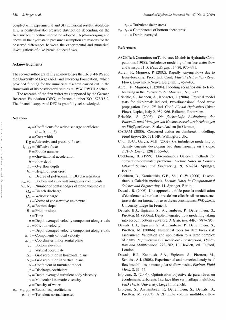
Figure 11 Unit discharge [m2/s] computed with FV model for testQ300-h50 with an elongated inflow channel

which the flow velocity is also small with a low inflow dischargeand a high initial water depth.

Since the equations of motion, in particular the k-ε turbulenceclosure, are transport equations, proper boundary conditionsneed to be prescribed notably at the inlet and possibly influencethe computational result further downstream in the simulationdomain. Therefore, the sensitivity of the simulation output withrespect to the length of the inlet channel was investigated.Two simulations (with and without k-ε turbulence closure) wererepeated for test Q300-h50 with a length of the inlet channelincreased by 10 m (Fig. 11). The flow remains essentially insen-sitive to the inlet channel length, since the variation in breachdischarge does not exceed 0.2%.

5.6 Influence of bed and wall roughness

It has been verified with both computational models that modify-ing the Manning coefficient for a channel bed roughness within0.005 < nb < 0.020 s/m1/3 has no significant effect on thebreach discharge (0.3%). Increasing the Manning coefficientabove 0.02 s/m1/3 would be unrealistic considering the flumematerial of smooth paintwork. Even a value of 0.05 s/m1/3 inthe framework of a channel roughness sensitivity analysis in theFE model leads to minor changes in the discharge split.

Similarly, the influence of wall roughness (Eq. (6)) wasinvestigated with the FV model. For test Q300-h50, Table 7compares values of computed breach discharges with two dif-ferent wall roughness coefficients (nw = 0.015 s/m1/3 and nw =0.030 s/m1/3) and without wall roughness. Again, the flow sen-sitivity was found to be weak, since the relative change in thebreach discharge does not exceed 1%. This slight increase in the



Table 7 Influence of wall roughness in test Q300-h50 simulated byFV model (algebraic turbulence closure α = 1)

Wall roughness None Moderate High

Coefficient nw [s/m1/3] 0.00 0.015 0.030Breach discharge [m3/s] 0.2014 0.2022 0.2035Relative change [%] 0.4 1.0

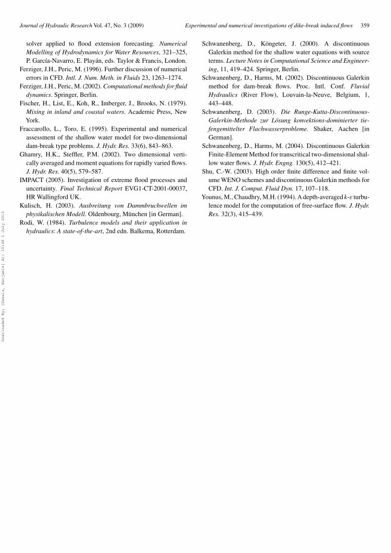
Figure 12 Unit discharges [m2/s] close to breach location, computedby FV model for test Q300-h50, (a) without wall roughness, (b) withwall roughness (nw = 0.030 s/m1/3)

breach discharge is associated with a change in the velocity profileand unit discharge in the channel immediately downstream of thebreach. Figure 12 compares the field of unit discharges obtainedwithout and with wall roughness. The latter is characterized bya wider area of lower velocity close to the right wall, leading toa flow constriction downstream of the breach and, therefore, anincrease in the breach discharge.

5.7 Influence of Boussinesq coefficients

Preliminary simulations were run with the FV model consider-ing spatially distributed Boussinesq coefficients (Eq. (5)). Theupwind scheme described in Section 4.2 was demonstrated toremain stable regardless of the value of the Boussinesq coeffi-cients (Dewals 2006). The CFL condition, however, needs to beupdated to account for its effect on wave celerity.

Results of these preliminary simulations demonstrate that theBoussinesq coefficients can indeed have a substantial influenceon the flow behavior. These simulations are based mainly onguesses regarding the distribution of the Boussinesq coefficientsand must be essentially considered as contributions to a sensitivityanalysis of the flow with respect to the Boussinesq coefficients.More realistic simulations can only be executed based on dis-tributions of Boussinesq coefficients inferred from experimentalmeasurements or 3D simulations. In such a framework, the 2Dmodeling relies on complementary experimental or 3D numericalmodeling, which is a weak point of such an approach. How-ever, a detailed analysis of 3D simulation results may lead to aparameterization of the Boussinesq coefficient as a function ofdepth-averaged flow characteristics (e.g. free surface curvature),which in turn makes the 2D model self-sufficient by adding a clo-sure relationship linking the local Boussinesq coefficient to theprimitive unknowns (or their derivative) of the depth averagedmodel.

Currently, velocity profiles over depth are available from mea-surements performed at IWW-RWTH for a restricted floodplainarea nearby the breach within the body of the wave (2.2). Dueto the distribution of horizontal velocity components u and v,the depth averaging yields high values of Boussinesq coeffi-cients, which actually cannot be applied in one-to-one for suchheterogeneous profiles.

A simulation with the FV model based simply on this distribu-tion of Boussinesq coefficients indicates a slight increase in thereleased discharge. Moreover, the real Boussinesq coefficientsare expected to differ from unity in a much wider area, includingthe channel in the breach vicinity. If this overall distribution istaken into account in depth-averaged modeling, the breach dis-charge might be much more affected. Therefore, 3D simulationsare presently undertaken at IWW-RWTH to provide 2D modelswith a reliable spatial distribution of Boussinesq coefficients inthe entire computational domain.

6 Conclusions

Both investigated 2D depth-averaged shallow-water modelsreproduce satisfactorily the basic flow pattern and the qualitativeflow split for different configurations of experimental dike-breakinduced flows. The flooding event is modeled from an initial statefor a closed flap gate in a single stable run, without oscillationsincluding the channel and the wave propagation area. This con-firms the convergence and general applicability of the methodsused for dike-break problems.

The resulting deviations from the performed measurementsincluding underestimation of breach discharges by 4% to 11%were analyzed focusing on the simplifications of the mathemati-cal model and the numerical approach. The applied CFD-methodsshould at least be of second order accuracy in space to minimizenumerical diffusion which otherwise affects the solution. Thetested simulations involve a low solution sensitivity as regardsturbulence modeling, bed and wall roughness. Accordingly,progress has to be made in the use of Boussinesq coefficients,



coupled with experimental and 3D numerical results. Addition-ally, a nonhydrostatic pressure distribution depending on thefree surface curvature should be adopted. Depth-averaging andabove all the hydrostatic pressure assumption are reasons for theobserved differences between the experimental and numericalinvestigations of dike-break induced flows.

Acknowledgments

The second author gratefully acknowledges the F.R.S.-FNRS andthe University of Liege (ARD and Duesberg Foundation), whichprovided funding for the numerical research carried out in theframework of his postdoctoral studies at IWW, RWTH Aachen.

The research of the first writer was supported by the GermanResearch Foundation (DFG), reference number KO 1573/15-2.The financial support of DFG is gratefully acknowledged.

Notation

ai = Coefficients for weir discharge coefficient(i = 0, . . . , 3)

b = Crest widthf, g =Advective and pressure fluxes

fd , gd = Diffusive fluxesF = Froude numberg = Gravitational accelerationh = Flow depth

ho = Overflow depthhw = Height of weir crestk = Degree of polynomial in DG discretization

nb, nw = Bottom and side-wall roughness coefficientsNx, Ny = Number of contact edges of finite volume cell

QB = Breach dischargeQw =Weir discharge

s =Vector of conservative unknownsSo = Bottom slopeSf = Friction slope

t = Timeu = Depth-averaged velocity component along x-axis

u∗ = Friction velocityv = Depth-averaged velocity component along y-axis

u, v = Components of local velocityx, y = Coordinates in horizontal plane

zb = Bottom elevationz =Vertical coordinate

�x = Grid resolution in horizontal plane�z = Grid resolution in vertical plane

α = Coefficient of turbulent modelµ = Discharge coefficientνt = Depth-averaged turbulent eddy viscosityν = Molecular kinematic viscosityρ = Density of water

ρxx, ρyy, ρxy = Boussinesq coefficientsσx, σy = Turbulent normal stresses

τxy = Turbulent shear stressτbx, τby = Components of bottom shear stress

〈·〉 = Depth-averaged

References

ASCE Task Committee on Turbulence Models in Hydraulic Com-putations (1988). Turbulence modeling of surface water flowand transport 1. J. Hydr. Engng. 114(9), 970–991.

Aureli, F., Mignosa, P. (2002). Rapidly varying flows due tolevee-breaking. Proc. Intl. Conf. Fluvial Hydraulics (RiverFlow), Louvain-la-Neuve, Belgium, 1, 459–466.

Aureli, F., Mignosa, P. (2004). Flooding scenarios due to leveebreaking in the Po river. Water Manage. 157, 3–12.

Briechle, S., Joeppen, A., Köngeter, J. (2004). Physical modeltests for dike-break induced, two-dimensional flood wavepropagation. Proc. 2nd Intl. Conf. Fluvial Hydraulics (RiverFlow), Naples, Italy 2, 959–966. Balkema, Rotterdam.

Briechle, S. (2006). Die flächenhafte Ausbreitung derFlutwelle nach Versagen von Hochwasserschutzeinrichtungenan Fließgewässern. Shaker, Aachen [in German].

CADAM (2000). Concerted action on dambreak modelling,Final Report SR 571, HR, Wallingford UK.

Choi, S.-U., Garcia, M.H. (2002). k-ε turbulence modelling ofdensity currents developing two dimensionally on a slope.J. Hydr. Engng. 128(1), 55–63.

Cockburn, B. (1999). Discontinuous Galerkin methods forconvection-dominated problems. Lecture Notes in Compu-tational Science and Engineering, 9, 69–224. Springer,Berlin.

Cockburn, B., Karniadakis, G.E., Shu, C.-W. (2000). Discon-tinuous Galerkin methods. Lecture Notes in ComputationalScience and Engineering, 11. Springer, Berlin.

Dewals, B. (2006). Une approche unifiée pour la modélisationd’écoulements à surface libre, de leur effet érosif sur une struc-ture et de leur interaction avec divers constituants. PhD thesis.University, Liege [in French].

Dewals, B.J., Erpicum, S., Archambeau, P., Detrembleur, S.,Pirotton, M. (2006a). Depth-integrated flow modelling takinginto account bottom curvature. J. Hydr. Res. 44(6), 787–795.

Dewals, B.J., Erpicum, S., Archambeau, P., Detrembleur, S.,Pirotton, M. (2006b). Numerical tools for dam break riskassessment: Validation and application to a large complexof dams. Improvements in Reservoir Construction, Opera-tion and Maintenance, 272–282, H. Hewlett, ed. Telford,London.

Dewals, B.J., Kantoush, S.A., Erpicum, S., Pirotton, M.,Schleiss, A.J. (2008). Experimental and numerical analysis offlow instabilities in rectangular shallow basins. Environ. FluidMech. 8, 31–54.

Erpicum, S. (2006). Optimisation objective de paramètres enécoulements turbulents à surface libre sur maillage multibloc.PhD Thesis. University, Liege [in French].

Erpicum, S., Archambeau, P., Detrembleur, S., Dewals, B.,Pirotton, M. (2007). A 2D finite volume multiblock flow



solver applied to flood extension forecasting. NumericalModelling of Hydrodynamics for Water Resources, 321–325,P. García-Navarro, E. Playán, eds. Taylor & Francis, London.

Ferziger, J.H., Peric, M. (1996). Further discussion of numericalerrors in CFD. Intl. J. Num. Meth. in Fluids 23, 1263–1274.

Ferziger, J.H., Peric, M. (2002). Computational methods for fluiddynamics. Springer, Berlin.

Fischer, H., List, E., Koh, R., Imberger, J., Brooks, N. (1979).Mixing in inland and coastal waters. Academic Press, NewYork.

Fraccarollo, L., Toro, E. (1995). Experimental and numericalassessment of the shallow water model for two-dimensionaldam-break type problems. J. Hydr. Res. 33(6), 843–863.

Ghamry, H.K., Steffler, P.M. (2002). Two dimensional verti-cally averaged and moment equations for rapidly varied flows.J. Hydr. Res. 40(5), 579–587.

IMPACT (2005). Investigation of extreme flood processes anduncertainty. Final Technical Report EVG1-CT-2001-00037,HR Wallingford UK.

Kulisch, H. (2003). Ausbreitung von Dammbruchwellen imphysikalischen Modell. Oldenbourg, München [in German].

Rodi, W. (1984). Turbulence models and their application inhydraulics: A state-of-the-art, 2nd edn. Balkema, Rotterdam.

Schwanenberg, D., Köngeter, J. (2000). A discontinuousGalerkin method for the shallow water equations with sourceterms. Lecture Notes in Computational Science and Engineer-ing, 11, 419–424. Springer, Berlin.

Schwanenberg, D., Harms, M. (2002). Discontinuous Galerkinmethod for dam-break flows. Proc. Intl. Conf. FluvialHydraulics (River Flow), Louvain-la-Neuve, Belgium, 1,443–448.

Schwanenberg, D. (2003). Die Runge-Kutta-Discontinuous-Galerkin-Methode zur Lösung konvektions-dominierter tie-fengemittelter Flachwasserprobleme. Shaker, Aachen [inGerman].

Schwanenberg, D., Harms, M. (2004). Discontinuous GalerkinFinite-Element Method for transcritical two-dimensional shal-low water flows. J. Hydr. Engng. 130(5), 412–421.

Shu, C.-W. (2003). High order finite difference and finite vol-ume WENO schemes and discontinuous Galerkin methods forCFD. Int. J. Comput. Fluid Dyn. 17, 107–118.

Younus, M., Chaudhry, M.H. (1994). A depth-averaged k-ε turbu-lence model for the computation of free-surface flow. J. Hydr.Res. 32(3), 415–439.


journal of hydraulic research experimental and numerical

Documents