Vol 6 Issue 2 • Sept 2014

Inside this issue

Improved ventilation to reduce formaldehyde exposure during wet anatomical classes

Development of a Tool for the Adjustment of Workplace Exposure Standards for Atmospheric Contaminants Due to Extended Work Shifts

Assessing airborne contaminant exposures during cold splicing and hot splicing of conveyor belts in the Western Australian mining sector

Stretching but not too far: Understanding adaptive behaviour using a model of organisational elasticity

Journal of

HEALTH and SAFETY

RESEARCH and

PRACTICE

A publication for members of the Safety Institute of Australia Ltd

Volume 6 Issue 2 • September 2014 JOURNAL OF HEALTH AND SAFETY, RESEARCH AND PRACTICE 1

IN THIS ISSUEImproved ventilation to reduce formaldehyde exposure during wet anatomical classes

Roy Schmid and Sarah Thornton — Pages 2–5

Development of a Tool for the Adjustment of Workplace Exposure Standards for Atmospheric Contaminants Due to Extended Work Shifts

Ian Firth and Daniel Drolet — Pages 6–10

Assessing airborne contaminant exposures during cold splicing and hot splicing of conveyor belts in the Western Australian mining sector

Teresa Smith, Jacques Oosthuizen, Sue Reed and John Yates — Pages 11–17

Stretching but not too far: Understanding adaptive behaviour using a model of organisational elasticityStephen Cowley and David Borys — Pages 18–22

Journal of

HEALTH and SAFETY

RESEARCH and

PRACTICEVol 6 Issue 2 • Sept 2014

Editorial BoardEDITOR IN CHIEF

Dr Stephen Cowley

EXECUTIVE EDITORSDr David Borys,

Dr Susanne Tepe

BOARD MEMBERSDr Liz Bluff

Dr Jenny JobDr Geoff Dell CFSIA Dr Felicity LammProfessor Niki Ellis

Prof. Rod McClure

Prof. Dennis Else FSIA (Hon)

Prof. Michael Quinlan FSIA

Dr Barry Gilbert FSIA Dr George Rechnitzer FSIA (Hon)

Prof. Andrew Hopkins FSIA Prof. Derek Smith FSIA

Derek Viner FSIA (Hon)

Guidelines for authors Guidelines for authors are available at www.sia.org.au

Subscriptions The journal is distributed free-of-charge to members of the Safety Institute of Australia.

Members may also access electronic copies of articles via www.sia.org.au. Published articles are available freely (open-source) via www.sia.org.au 6 months after publication. Subscribers will receive printed copies of each volume

of the journal at the time of publication and will be granted access to the electronic copies of the latest articles. In addition to receiving the JHSRP, subscribers will also receive the OHS Professional magazine,

which is published quarterly. Subscriptions rates are available via www.sia.org.au.

CorrespondenceCorrespondence should sent to: The Editor in Chief Journal of Health & Safety Research & Practice, Safety

Institute of Australia Ltd. PO Box 2078, Gladstone Park, Victoria 3043. Email: publications@sia.org.au ISSN 1837-5030The JHSRP is an international publication of the Safety Institute of Australia Ltd.

It is aimed at health and safety practitioners, researchers and students.

The journal aims to: > Promote evidence and knowledge-based practice

in health and safety;

> Share information about health and safety interventions;

> Share information about solutions to health and safety problems;

> Encourage intellectual debate around propositions for improvements in practice.

All published papers have been subjected to a double-blind refereeing process by at least two referees.

The journal is distributed free-of-charge to members of the Safety Institute of Australia.

Members may also access electronic copies of articles via www.sia.org.au.

Published articles are available freely (open-source) via www.sia.org.au 6 months after publication.

2 JOURNAL OF HEALTH AND SAFETY, RESEARCH AND PRACTICE Volume 6 Issue 2 • September 2014

CITE THIS ARTICLE ASSchmid, R. & Thornton, S., (2014), Improved ventilation to reduce formaldehyde exposure during wet anatomical classes, J Health & Safety Research & Practice 6(2), 2-5.

KEYWORDSFormaldehyde, local exhaust ventilation, anatomy laboratory, teaching

CORRESPONDENCE OHS Branch, Work Environment Group The Australian National University CanberraEmail: Sarah.Thornton@anu.edu.au

1 The Australian National University

Improved ventilation to reduce formaldehyde exposure during wet anatomical classesMr Roy Schmid1 and Ms Sarah Thornton1

AbstractA University Medical School began offering anatomy classes in 2002, in a space not originally designed as a wet laboratory. When Anatomy classes began using wet specimens, fixed in a solution that contains 4-5% formalin, vapours of formaldehyde were released. Formaldehyde can cause irritant effects at very low levels and the International Agency for Research on Cancer has classified formaldehyde as carcinogenic to humans (group 1). The current Australian classification is Category 2 – probable human carcinogen for which there is sufficient evidence to provide a strong presumption that human exposure might result in the development of cancer. The current Australian exposure standard is 1 ppm with a STEL of 2 ppm. Proposed exposure standards are lower to control irritant effects.

Over the past 11 years in conjunction with monitoring and recommendations by the University’s Occupational Health and Safety Branch there has been a gradual improvement in conditions in the teaching laboratory. Most recently, through consultation with users of the area, Facilities and Services Division and consultants, a local exhaust ventilation system was designed and installed. Formaldehyde vapours are now removed as they are generated, with minimal restrictions on student access to the specimens.

This paper presents the results of various monitoring sessions over the years 2004-2013, along with discussion of the types of controls considered, design of the ventilation system and follow-up monitoring results. The objective of minimising student exposure and protecting their health has been achieved.

IntroductionAnatomy classes at the ANU Medical School incorporate the dissection of human cadavers preserved in commercial anatomical arterial mixture (embalming fluid) containing formaldehyde. During the dissection, staff and students are exposed to formaldehyde.

The commercial Anatomical Arterial Mixture (Hickey & Company, 2008) (embalming solution) contains 4-5% formaldehyde, 2% methanol and 6% isopropanol. Although other hazards exist with this product only the inhalation toxicity of the formaldehyde vapour is considered in this paper.

Formaldehyde is readily absorbed by all routes of exposure. When inhaled, it reacts rapidly at the site of contact and is quickly metabolised in the respiratory tissue. Formaldehyde is a human irritant in air at levels above 0.5 ppm (lowest observed effect level, LOEL), while 0.8

ppm is the typical level of perception (NICNAS, 2006a). Above these levels irritation increases substantially up to 20 ppm, at which it is immediately dangerous to life and health (NIOSH 2013).

Sensitisation to formaldehyde can develop when a person is exposed through skin contact, while gaseous formaldehyde is unlikely to induce human respiratory sensitisation. There is limited evidence that indicates that formaldehyde may elicit a respiratory response in some very sensitive individuals with bronchial hyperactivity, probably through irritation of the airways (NICNAS, 2006).

Systemic toxicity is not observed following repeated exposure to formaldehyde. Based on animal studies, formaldehyde is unlikely to cause reproductive and developmental effects at exposures relevant to humans (NICNAS, 2006b).

Formaldehyde is considered to have a weak genotoxic potential. The International Agency for Research on Cancer (IARC) concluded that there is sufficient evidence (epidemiological studies) that formaldehyde causes nasopharyngeal cancer in humans Cancer (IARC 2006). IARC has classified formaldehyde as carcinogenic to humans (group 1). The current Australian classi-fication is Category 2 – probable human carcinogen for which there is sufficient evidence to provide a strong presumption that human exposure might result in the development of cancer (Safe Work Australia 2013). Further information on formaldehyde exposures can be found in the National Industrial Chemicals Notifica tion and Assessment Scheme (NICNAS) Priority Existing Chemical Assessment Report (NICNAS, 2006a) and associated Safety Information Sheets (NICNAS, 2006b).

The anatomy classes have steadily grown in size over the years, now reaching 50 students.

Preserved specimens are removed from large storage tubs at the beginning of the practical session, and later returned by laboratory staff. These tubs contain a large volume of anatomical arterial mixture. Tubs are opened in another limited occupancy ventilated room,

Volume 6 Issue 2 • September 2014 JOURNAL OF HEALTH AND SAFETY, RESEARCH AND PRACTICE 3

releasing a large amount of formaldehyde. This process is being reviewed.

The Anatomical Arterial Mixture (Hickey & Company, 2008) is considered a low formaldehyde product, and less than previous generation embalming fluids. There have been unsuccessful attempts to find a safer (lower or zero formaldehyde) product.

Practical classes are typically 2 hours in duration. Students work on the preserved specimens for most of that time, while staff may be exposed for additional time (approximately 30 minutes during setup and clean-up). Dissection and handling of the specimens is satisfactorily undertaken using latex or nitrile gloves, surgical masks, disposable plastic aprons and safety glasses. The surgical masks assist in the removal of bioaerosols providing no protection against formaldehyde inhalation.

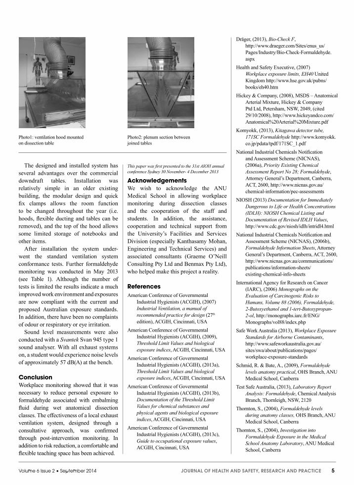
In May 2013 classes moved to a new laboratory. The early anatomy laboratories relied on dilution ventilation. The room was heated and cooled via the building ventilation system with ceiling mounted supply and return air grills. A low and high level exhaust grill was next to the entrance door. On several occasions odours circulated to other areas of the building. The windows in these laboratories are sealed shut for security reasons. The new laboratory contains nine stainless steel double sided ventilated benches with clear Perspex sides and top providing sufficient light and access for students to the specimens. (See photo 1).

This paper reports the findings of formaldehyde-in-air sampling in the early laboratories and the new laboratory between June 2004 and May 2013.

Workplace evaluationThe Australian occupational exposure standard 8-hour Time Weighted Average (TWA) for formaldehyde is currently 1 ppm, with a Short Term Exposure Limit (STEL) of 2 ppm (Safe Work Australia 2013). There is no appropriate peak limitation.

The American Conference of Govern-mental Hygienists (ACGIH) exposure standard is a ceiling (peak) limit of 0.3 ppm to control upper respiratory tract

irritation and eye irritation (ACGIH 2009, 2013a, 2013b). A ceiling limit is the maximum concentration of the substance that may be reached at any time. The United Kingdom workplace exposure standard TWA for formaldehyde is currently 2 ppm, with a STEL of 2 ppm (HSE 2007).

The Australian exposure standard for formaldehyde was reviewed in July 2012, and remains at 1 ppm, with a STEL of 2 ppm (Safe Work Australia 2013). However, the National Industrial Chemicals Notification and Assessment Scheme NICNAS review into formaldehyde (NICNAS 2006a), recommends lowering the exposure standard to 0.3 ppm 8 hr TWA and a 0.6 ppm STEL. This would also be more consistent with international standards (ACGIH 2013c). NICNAS believe that the new standard will offer adequate worker protection against discomfort (sensory irritation) but also provides a higher degree of cancer risk reduction (NICNAS 2006a). The University’s exposure standard target was therefore a TWA of 0.3 ppm and STEL of 0.6 ppm.

Between 2004 and 2013 a combination of sampling techniques were employed to determine formaldehyde concentrations and compliance with exposure standards. These ranged from detector tubes (komyokk 2013) and formaldehyde badges (Dräger 2013), to more precise active sampling with impregnated filters.

Kitagawa formaldehyde detector tubes (171SC) (komyokk 2013) provided a ‘snapshot’ concentration. Samples were taken at a height of about 1.5 m from the floor near the specimen bench. Sampling of this nature is not necessarily indicative of breathing zone exposures, although attempts were made to collect air in typical people locations.

Personal exposures were monitored using Dräger Bio-Check Formaldehyde instant tests (PZN 4898239) (Dräger 2013) placed in the breathing zone of volunteer staff and students. These tests passively monitored approximate concentration of formaldehyde, with little interference. Typically a badge was worn by students for the entire duration of a class.

Active sampling exposure monitoring

was carried out using 2,4 dinitrophenyl hydrazine (DNPH) impregnated 25 mm Pall glass fibre filters attached to an SKC Universal Portable Air Sampling Pump. The pumps were worn on the belt or waistband of a student with the filter head clamped to the clothes in the student’s breathing zone. The sampling flow rate was set at approximately half a litre per minute (500 ml/min) and the pumps were typically run for 30 minutes. The formaldehyde in the air reacts with the DNPH. Filters were sent to a NATA approved laboratory for analysis (Test Safe Australia 2013). Concentrations were reported for the session (column 4 of table 1), while some of these workplace concentrations were calculated out as 8-hour time weighted averages (column 6 of table 1).

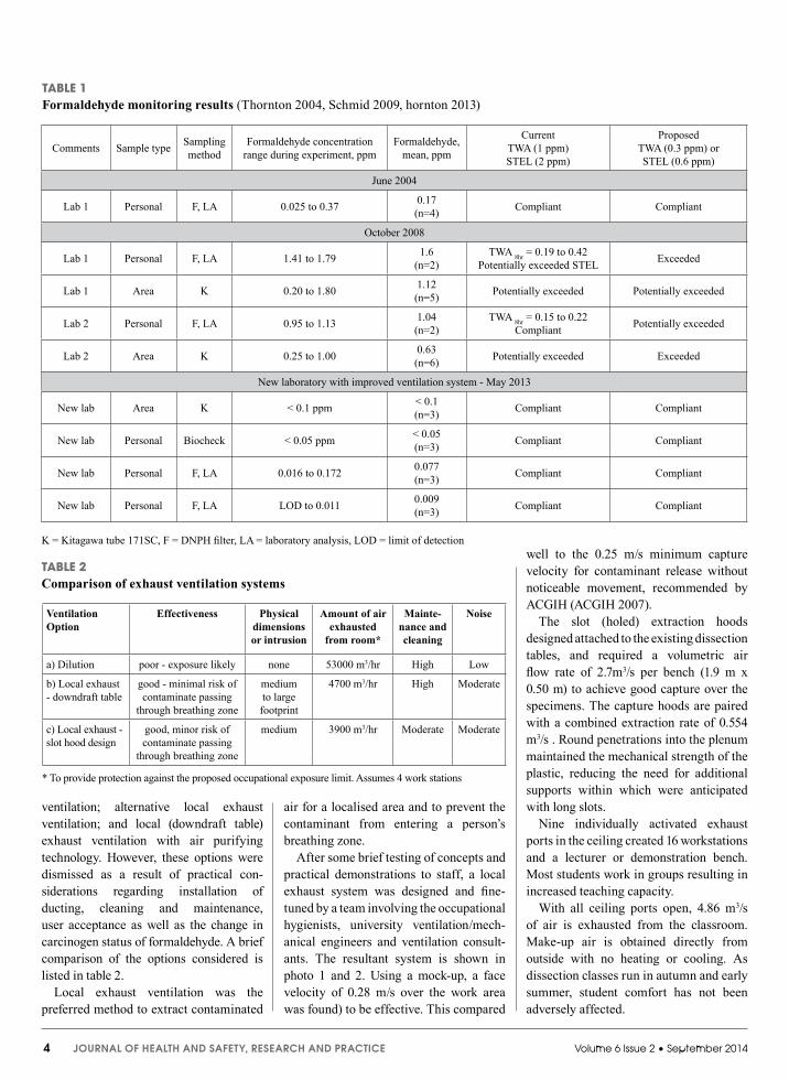
A summary of significant formaldehyde monitoring results are indicated in table 1. (See following Page)

DiscussionThe early results (2004) from small groups undertaking a relatively short (2 hour) practical session resulted in the concentration of formaldehyde almost never exceeding a person’s 8-hour exposure limit. However, as class sizes grew after 2007, work environment concentrations and personal exposures increased and the risk of non-compliance with current and proposed exposure standards was more plausible. In particular the short-term exposure limit (STEL of 0.6 ppm), could be regularly exceeded. These findings resulted in a number of activities that aimed to reduce exposure to formaldehyde.

Short term attempts to replace and reduce anatomy fixative solution were of little success, with tissue samples rotting faster than acceptable without the formaldehyde fixative. Therefore significant effort was put into improving the ventilation system. Several options were explored including improving the old laboratory’s dilution ventilation. However, this was quickly dismissed owing to both the realisation that a larger classroom was required and the anticipated change in carcinogen status of formaldehyde; Other considerations were the provision of; commercial (downdraft table) exhaust

4 JOURNAL OF HEALTH AND SAFETY, RESEARCH AND PRACTICE Volume 6 Issue 2 • September 2014

well to the 0.25 m/s minimum capture velocity for contaminant release without noticeable movement, recommended by ACGIH (ACGIH 2007).

The slot (holed) extraction hoods designed attached to the existing dissection tables, and required a volumetric air flow rate of 2.7m3/s per bench (1.9 m x 0.50 m) to achieve good capture over the specimens. The capture hoods are paired with a combined extraction rate of 0.554 m3/s . Round penetrations into the plenum maintained the mechanical strength of the plastic, reducing the need for additional supports within which were anticipated with long slots.

Nine individually activated exhaust ports in the ceiling created 16 workstations and a lecturer or demonstration bench. Most students work in groups resulting in increased teaching capacity.

With all ceiling ports open, 4.86 m3/s of air is exhausted from the classroom. Make-up air is obtained directly from outside with no heating or cooling. As dissection classes run in autumn and early summer, student comfort has not been adversely affected.

ventilation; alternative local exhaust ventilation; and local (downdraft table) exhaust ventilation with air purifying technology. However, these options were dismissed as a result of practical con-siderations regarding installation of ducting, cleaning and maintenance, user acceptance as well as the change in carcinogen status of formaldehyde. A brief comparison of the options considered is listed in table 2.

Local exhaust ventilation was the preferred method to extract contaminated

air for a localised area and to prevent the contaminant from entering a person’s breathing zone.

After some brief testing of concepts and practical demonstrations to staff, a local exhaust system was designed and fine-tuned by a team involving the occupational hygienists, university ventilation/mech-anical engineers and ventilation consult-ants. The resultant system is shown in photo 1 and 2. Using a mock-up, a face velocity of 0.28 m/s over the work area was found) to be effective. This compared

TABLE 1Formaldehyde monitoring results (Thornton 2004, Schmid 2009, hornton 2013)

Comments Sample type Sampling method

Formaldehyde concentration range during experiment, ppm

Formaldehyde, mean, ppm

CurrentTWA (1 ppm)STEL (2 ppm)

ProposedTWA (0.3 ppm) or STEL (0.6 ppm)

June 2004

Lab 1 Personal F, LA 0.025 to 0.37 0.17(n=4) Compliant Compliant

October 2008

Lab 1 Personal F, LA 1.41 to 1.79 1.6(n=2)

TWA 8hr = 0.19 to 0.42Potentially exceeded STEL Exceeded

Lab 1 Area K 0.20 to 1.80 1.12(n=5) Potentially exceeded Potentially exceeded

Lab 2 Personal F, LA 0.95 to 1.13 1.04(n=2)

TWA 8hr = 0.15 to 0.22Compliant Potentially exceeded

Lab 2 Area K 0.25 to 1.00 0.63(n=6) Potentially exceeded Exceeded

New laboratory with improved ventilation system - May 2013

New lab Area K < 0.1 ppm < 0.1(n=3) Compliant Compliant

New lab Personal Biocheck < 0.05 ppm < 0.05(n=3) Compliant Compliant

New lab Personal F, LA 0.016 to 0.172 0.077(n=3) Compliant Compliant

New lab Personal F, LA LOD to 0.011 0.009(n=3) Compliant Compliant

K = Kitagawa tube 171SC, F = DNPH filter, LA = laboratory analysis, LOD = limit of detection

Ventilation Option

Effectiveness Physical dimensions or intrusion

Amount of air exhausted

from room*

Mainte-nance and cleaning

Noise

a) Dilution poor - exposure likely none 53000 m3/hr High Low

b) Local exhaust - downdraft table

good - minimal risk of contaminate passing

through breathing zone

medium to large footprint

4700 m3/hr High Moderate

c) Local exhaust - slot hood design

good, minor risk of contaminate passing

through breathing zone

medium 3900 m3/hr Moderate Moderate

* To provide protection against the proposed occupational exposure limit. Assumes 4 work stations

TABLE 2Comparison of exhaust ventilation systems

Volume 6 Issue 2 • September 2014 JOURNAL OF HEALTH AND SAFETY, RESEARCH AND PRACTICE 5

The designed and installed system has several advantages over the commercial downdraft tables. Installation was relatively simple in an older existing building, the modular design and quick fix clamps allows the room function to be changed throughout the year (i.e. hoods, flexible ducting and tables can be removed), and the top of the hood allows some limited storage of notebooks and other items.

After installation the system under-went the standard ventilation system conformance tests. Further formaldehyde monitoring was conducted in May 2013 (see Table 1). Although the number of tests is limited the results indicate a much improved work environment and exposures are now compliant with the current and proposed Australian exposure standards. In addition, there have been no complaints of odour or respiratory or eye irritation.

Sound level measurements were also conducted with a Svantek Svan 945 type 1 sound analyser. With all exhaust systems on, a student would experience noise levels of approximately 57 dB(A) at the bench.

ConclusionWorkplace monitoring showed that it was necessary to reduce personal exposure to formaldehyde associated with embalming fluid during wet anatomical dissection classes. The effectiveness of a local exhaust ventilation system, designed through a consultative approach, was confirmed through post-intervention monitoring. In addition to risk reduction, a comfortable and flexible teaching space has been achieved.

This paper was first presented to the 31st AIOH annual conference Sydney 30 November- 4 December 2013

AcknowledgementsWe wish to acknowledge the ANU Medical School in allowing workplace monitoring during dissection classes and the cooperation of the staff and students. In addition, the assistance, cooperation and technical support from the University’s Facilities and Services Division (especially Kanthasamy Mohan, Engineering and Technical Services) and associated consultants (Graeme O’Neill Consulting Pty Ltd and Benmax Pty Ltd), who helped make this project a reality.

ReferencesAmerican Conference of Governmental

Industrial Hygienists (ACGIH), (2007) Industrial Ventilation, a manual of recommended practice for design (27th edition), ACGIH, Cincinnati, USA

American Conference of Governmental Industrial Hygienists (ACGIH), (2009), Threshold Limit Values and biological exposure indices, ACGIH, Cincinnati, USA

American Conference of Governmental Industrial Hygienists (ACGIH), (2013a), Threshold Limit Values and biological exposure indices, ACGIH, Cincinnati, USA

American Conference of Governmental Industrial Hygienists (ACGIH), (2013b), Documentation of the Threshold Limit Values for chemical substances and physical agents and biological exposure indices, ACGIH, Cincinnati, USA

American Conference of Governmental Industrial Hygienists (ACGIH), (2013c), Guide to occupational exposure values, ACGIH, Cincinnati, USA

Dräger, (2013), Bio-Check F, http://www.draeger.com/Sites/enus_us/Pages/Industry/Bio-Check-Formaldehyde.aspx

Health and Safety Executive, (2007) Workplace exposure limits, EH40 United Kingdom http://www.hse.gov.uk/pubns/books/eh40.htm

Hickey & Company, (2008), MSDS – Anatomical Arterial Mixture, Hickey & Company Ptd Ltd, Petersham, NSW, 2049, (cited 29/10/2008), http://www.hickeyandco.com/Anatomical%20Arterial%20Mixture.pdf

Komyokk, (2013), Kitagawa detector tube, 171SC Formaldehyde http://www.komyokk.co.jp/pdata/tpdf/171SC_1.pdf

National Industrial Chemicals Notification and Assessment Scheme (NICNAS), (2006a), Priority Existing Chemical Assessment Report No 28; Formaldehyde, Attorney General’s Department, Canberra, ACT, 2600, http://www.nicnas.gov.au/chemical-information/pec-assessments

NIOSH (2013) Documentation for Immediately Dangerous to Life or Health Concentrations (IDLH): NIOSH Chemical Listing and Documentation of Revised IDLH Values, http://www.cdc.gov/niosh/idlh/intridl4.html

National Industrial Chemicals Notification and Assessment Scheme (NICNAS), (2006b), Formaldehyde Information Sheets, Attorney General’s Department, Canberra, ACT, 2600, http://www.nicnas.gov.au/communications/publications/information-sheets/existing-chemical-info-sheets

International Agency for Research on Cancer (IARC), (2006) Monographs on the Evaluation of Carcinogenic Risks to Humans, Volume 88 (2006), Formaldehyde, 2-Butoxyethanol and 1-tert-Butoxypropan-2-ol, http://monographs.iarc.fr/ENG/Monographs/vol88/index.php

Safe Work Australia (2013), Workplace Exposure Standards for Airborne Contaminants, http://www.safeworkaustralia.gov.au/sites/swa/about/publications/pages/workplace-exposure-standards

Schmid, R. & Bate, A., (2009), Formaldehyde levels anatomy practical, OHS Branch, ANU Medical School, Canberra

Test Safe Australia, (2013), Laboratory Report Analysis: Formaldehyde, Chemical Analysis Branch, Thornleigh, NSW, 2120

Thornton, S., (2004), Formaldehyde levels during anatomy classes, OHS Branch, ANU Medical School, Canberra

Thornton, S., (2004), Investigation into Formaldehyde Exposure in the Medical School Anatomy Laboratory, ANU Medical School, Canberra

Photo1: ventilation hood mounted on dissection table

Photo2: plenum section between joined tables

6 JOURNAL OF HEALTH AND SAFETY, RESEARCH AND PRACTICE Volume 6 Issue 2 • September 2014

IntroductionThe American Conference of Govern-mental Industrial Hygienists (ACGIH®) and Safe Work Australia (SWA) have in the past recommended the use of the Brief & Scala (1975) correction model for adjusting Workplace Exposure Standards (WES) for extended work schedules. Since 2004 however, the ACGIH® has also referred to the Quebec Model jointly developed by the University of Montréal and the Institut de recherche Robert-Sauvé en santé et en sécurité du travail (IRSST), emphasising that it generates results closer to the physiologically-based toxicokinetic models (PBPK) than the Brief & Scala model.

In a position paper “Adjustment of Workplace Exposure Standards for Extended Work Shifts” (AIOH 2013), first published in 2010, the Australian Institute of Occupational Hygienists (AIOH) recommended a move to a model similar to that of the Québec model. This model is computer-based and utilises current toxicological information and can provide consistent guidance. It initially led to the development of an Excel tool based on that of the IRSST (Drolet, 2008) using Safe Work Australia workplace exposure standards tables that had been

assigned adjustment factors by the AIOH Exposure Standards Committee.

This paper provides a brief overview of discussions with SWA and reports the work of the AIOH Exposure Standards Committee on the development of a Microsoft Excel tool that facilitates the adjustment of SWA WESs for extended shifts, providing a choice of either the Québec model or the Brief and Scala model according to a specific logic tree.

Safe Work Australia DocumentationSections 17 and 19 of the model Work Health and Safety (WHS) Act (SWA, 2011) together require that exposure to substances in the workplace is kept as low as is reasonably practicable. Under the WHS Regulations (SWA, 2014), a person who conducts a business or undertaking (PCBU) must:• manage risks under the WHS

Regulations, including those associated with using, handling and storing hazardous chemicals safely, airborne contaminants and asbestos;

•ensure that no person at the workplace is exposed to a substance or mixture in an airborne concentration that exceeds the exposure standard for the substance or mixture (r 49); and

•ensure that air monitoring is carried out to determine the airborne concentra tion of a substance or mixture at the workplace to which an exposure standard applies if:o the person is not certain on reasonable

grounds whether or not the airborne concentration of the substance or mixture at the workplace exceeds the relevant exposure standard, or

o monitoring is necessary to determine whether there is a risk to health (r 50).

Safe Work Australia has produced the document “Workplace Exposure Standards for Airborne Contaminants” (SWA, 2013b), containing a list of workplace exposure standards (WES) for airborne contaminants and how to meet PCBU duties under the WHS Act and the WHS Regulations. It is a supplement to the Hazardous Substances Information System (HSIS; SWA, 2013a), which is available on the SWA website.

CITE THIS ARTICLE AS Firth, I. & Drolet, D., (2014), Development of a Tool for the Adjustment of Workplace Exposure Standards for Atmospheric Contaminants Due to Extended Work Shifts, J Health & Safety Research & Practice 6(2), 6-10.

KEYWORDSExposure standard, adjustment, extended work shift

CORRESPONDENCEIan FirthPO Box 1205 Tullamarine Vic 3043 Email: ian.firth55@gmail.com

1 AIOH Workplace Exposure Standards Committee volunteer

Development of a Tool for the Adjustment of Workplace Exposure Standards for Atmospheric Contaminants Due to Extended Work ShiftsIan Firth1 and Daniel Drolet1

AbstractAn Australian Institute of Occupational Hygienists (AIOH) position paper “Adjustment of Workplace Exposure Standards for Extended Work Shifts” provided an overview of the workplace exposure standard (WES) adjustment methods for atmospheric contaminants. It concluded that the current guidelines provided by Safe Work Australia (SWA) were inadequate in that they did not consider or accommodate the varying range of health effects of different agents and their time frame for adverse effect and could lead to inconsistent advice for affected workers. The AIOH recommended moving to a model similar to that of the Québec model and developed a tool that provides an appropriate and accessible methodology to adjust exposure standards for extended work shifts and thus more consistent and informed advice for affected workers.

Volume 6 Issue 2 • September 2014 JOURNAL OF HEALTH AND SAFETY, RESEARCH AND PRACTICE 7

SWA has also produced the document “Guidance on the interpretation of workplace exposure standards for airborne contaminants” (SWA, 2013c), which provides more detailed information about the application of exposure standards.

A WES, the airborne concentration of a particular substance or mixture that must not be exceeded, can be a; 8-hour time-weighted average (TWA); peak limitation (similar to a ceiling value); and / or short term exposure limit (STEL).

SWA (2013b) clearly states,“Where workers have a working day longer than eight hours or work more than 40 hours a week, the per-son conducting the business or un-dertaking must determine whether the TWA exposure standard needs to be adjusted to compensate for the greater exposure during the longer work shift, and decreased recovery time between shifts. Peak limitation or Short Term Exposure Limit ex-posure standards must not be adjust-ed. 8-Hour TWA exposure standards must not be adjusted (increased) for shorter work shifts.”

SWA (2013c) currently mentions several different methods for adjusting WES, but recommends use of the Brief & Scala method for its simplicity of use and conservatism. However, there is currently a recommendation to update the “Guidance on the interpretation of workplace exposure standards for airborne contaminants” document such that it recommends use of either the Québec or the Brief & Scala models, supported by an on-line / computer-based tool, the Australianised Québec model.

Québec ModelThe Québec model is based on the guiding principle of “…ensuring an equivalent degree of protection to workers with a conventional schedule of 8 hours a day, 5 days a week, and to workers with unusual work schedules” and uses the logic of the Occupational Safety and Health Administration (OSHA) (Paustenbach, 1994) (the OSHA model). IRSST and University of Montréal toxicologists

proposed adjustment categories (Table 1) for each of the substances found in Schedule I of the Quebec Regulation respecting occupational health and safety (ROHS), as well as a method for calculating adjustment factors supported by toxicokinetic modeling. This group of experts also defined the conditions and limitations of application of the adjustment procedure (Drolet, 2008).

TABLE 1List of adjustment categories for the Quebec model (as also proposed by OSHA)Adj Adjustment

classification Type of adjustment

1A Substances regulated by a ceiling value

No adjustment

1B Irritating or malodorous substances

1C Simple asphyxiants, substances presenting a safety risk or a very low health risk, whose half-life is less than 4 hours. Technological limitations

2 Substances that produce effects following short-term exposure

Daily adjustment

3 Substances that produce effects following long-term exposure

Weekly adjustment

4 Substances that produce effects following short- or long-term exposure

Daily or weekly adjustment the most conser vative of the two

In the case of Category 1 substances, the time-weighted average exposure standard (TWAES) does not have to be adjusted, regardless of the type of work schedule. Values for short term exposure limits (STELs) and ceiling or peak limits are not subject to the adjustment principle; only the TWAESs are subject to the adjustment principle. For substances belonging to the other categories, the TWAES is adjusted by applying one of the following equations: Fa = 8/Hd Category 2 substances,

requiring a daily adjustment,

Fa = 40/Hwk Category 3 substances, requiring a weekly adjustment,

Where: Fa = adjustment factor Hd = exposure duration in

hours per shift Hwk = average duration of

work shifts per week based on a repetitive work cycle.

In the case of Category 4 substances, the Fa must be calculated for each of the two equations for Categories 2 and 3, and the lowest Fa must be applied. It should be noted that the above-mentioned computer-based tool automatically calculates the adjusted average exposure value (AAEV) from the most conservative Fa.

The TWAES adjustment process applies only to nominal schedules with shifts of no less than 4 hours and no more than 16 hours and in no case can the AAEV be greater than the TWAES. It should also be noted that OEL adjustment is based on the toxicological knowledge available in the scientific and technical literature.

The IRSST guidance document (Drolet, 2008) should be referred to for relevant definitions and other documentation of the Québec model.

Australian Workplace Exposure StandardsThere are currently 673 WES for a range of substances (and mixtures) in the document “Workplace Exposure Standards for Airborne Contaminants” (SWA, 2013b) and in the HSIS (SWA, 2013a). The great majority of these were adopted from the ACGIH®, updated to reflect the values published by the ACGIH® in 1994. Between 1998 and 2005, eighty WES reviews were undertaken. The vast majority of these involved the adoption of British Health and Safety Executive (HSE) exposure standards or the National Industrial Chemical Notification and Assessment Scheme (NICNAS) Priority Existing Chemical (PEC) Report recommendations. The last update of the WESs was in August 2005, when 31 substances were amended using the fourth batch of Source A updates adopted from the British HSE and the first batch of Source A updates adopted from the NICNAS PEC report recommendations (SWA, 2013a).

There are a number of WESs that are higher than the exposure standards for other countries (eg. the arsenic and

8 JOURNAL OF HEALTH AND SAFETY, RESEARCH AND PRACTICE Volume 6 Issue 2 • September 2014

1,3-butadiene WESs are five times higher than their respective ACGIH® Threshold Limit Value (TLV®)), as well as a number that are lower (eg. the chloroform WES is five times lower than the TLV®), and there are many international exposure standards not represented in the WESs. There are also some WESs that are not represented in Schedule I of the Québec Regulations that were compared for determination of an appropriate adjustment category (AC).

A key point to note then is that a number of the Australian WESs have not been reviewed for a number of years, hence may not reflect the most recent research on health effects due to exposures in the workplace. In assigning an appropriate adjustment category (AC)to each of the Australian WESs during the work reported herein, there was no intent to also update the WES itself. Current documentation was reviewed in order to assign the most appropriate AC with regard to health effects, as detailed in the next section.

The Australianised Québec ModelThe starting point for developing the Australianised Québec model was to take the assigned adjustment category (AC) for each of the substances in Schedule I of the Québec Regulation (Drolet, 2008) and match these to corresponding substances in the list of Australian WESs from “Workplace Exposure Standards for Airborne Contaminants” (SWA, 2013b). This was thought to be the best approach as this was the most recent such assignment of ACs. Where there was no matching substance, end point health effects and toxicology were used to derive the adjustment category assignment.

Once ACs were thus assigned, the following processes were undertaken to determine the need for modification of the “Québec model” IRSST ACs:A. WESs with a peak limitation (43

substances) were identified and assigned an AC = 1A. Not all ROHS listed substances with a peak limitation (ceiling limit) had a corresponding WES with such a limit, and vice versa.

B. WESs with a carcinogen designation

(Carc. 1A - known to have carcinogenic potential for humans; and Carc. 1B - presumed to have carcinogenic potential for humans) were identified and assigned an AC = 3 or 4, except for LPG, which retained its AC = 1C. A Carc.2 (suspected human carcinogen) designation did not usually elicit a change to the existing AC.

C. WESs with a sensitiser designation were identified and assigned an AC = 2, 3 or 4, except for Benzoyl peroxide, which retained its AC = 1B.

D. Selected WESs were reviewed by the Exposure Standards committee members and adjusted if the more recent documented health effects (ACGIH, 2011 & 2013) suggested a different AC.

Recent ACGIH® documentation (ACGIH, 2011), and health effects as listed in the 2013 ACGIH® TLV® booklet (ACGIH, 2013), were used to help validate proposed AC changes to those published by the IRSST (Drolet, 2008). Another list of assigned ACs based on the OSHA model, developed from the “Desktop Guide to Adjusting TLVs”, which was based on a review of the Documentation for the chemicals in the 6th Edition of Documentation of the Threshold Limit Values and Biological Exposure Indices published by the ACGIH® (Wylie, 2008), was also used to help validate any proposed changes.

There were a number of substances where the ACGIH® TLV® and the WES were so disparate, largely due to the WES being old, that it was difficult to discern whether the TLV® gave useful information on the sentinel effect used for developing the WES. In addition, the ‘TLV® basis’ in the booklet (ACGIH, 2013) did not always accurately reflect the documentation detail (ACGIH, 2011).

For several substances it was difficult to understand the conclusions drawn from the documentation. For a number of substances, there was limited documentation, often based solely on animal studies (e.g. the various pesticides). As an example cyclohexene, with an AC = 1B, has a TLV® of 300 ppm based on upper respiratory tract (URT) and eye irritation. The introductory

paragraph reads: “A TLV–TWA® of 300 ppm (1010 mg/m3) is recommended for occupational exposure to cyclohexene, in part by analogy with cyclohexane (see TLV® Documentation for Cyclohexane). This value is intended to minimize the potential for eye and mucous membrane irritation, based on limited data.” The cyclohexane TLV® documentation barely mentions irritation and at least two of the half dozen or so times that irritation is mentioned make the point that it does NOT happen at levels of interest. In these cases professional opinion was used to decide the AC.

A working sheet that documents AC decisions is maintained in an Excel spreadsheet kept by the AIOH Exposure Standards committee.

Brief and Scala ModelBrief & Scala (1975) proposed a “simple system” for adjusting the TLVs® for “novel work schedules”. A reduction factor (adjustment factor - Fa) for reducing the TLV® for a novel work schedule is to be calculated using the following equation:

Daily adjustment: Fa = (8 / Hd) x (24 - Hd / 16)

Where: Fa = adjustment factor

Hd = exposure duration in hours per shift

They suggest that the Fa value should be applied to; TLVs® expressed as a TWAES with respect to the mean and permissible excursion; and TLVs® that have a ceiling (peak) value, except where the peak limitation is based solely on sensory irritation. They suggest that in this case the irritation response threshold is not likely to be altered downward by an increase in number of hours worked and modification of the TLV® is not needed.

They then state that the Fa value should be applied to TLVs® that are based on systemic effect (acute or chronic). Acute effects are viewed as falling into two categories: (a) rapid with immediate onset and (b) manifest with time during a single exposure. They suggest that “the former are guarded by the C notation and the latter are presumed

Volume 6 Issue 2 • September 2014 JOURNAL OF HEALTH AND SAFETY, RESEARCH AND PRACTICE 9

time and concentration dependent and hence, are amenable to the modifications proposed.” STELs are not mentioned, but are presumed to be thus included in the adjustment process.

The number of days worked per week is not considered, except in the special case of a 7-day workweek. In this case the

Fa value is calculated as follows:

Weekly adjustment: Fa = (40 / Hwk) x (168 - Hwk / 128)

Where:Fa = adjustment factor

Hwk = average duration of work shifts per week based on a repetitive

work cycle.

The Exposure Standards committee decided to only apply an adjustment factor to OELs for those substances that have a long-term chronic effect, in alignment with good occupational hygiene practice (Paustenbach, 1994) and SWA suggested practice. That is, no adjustment was made to peak and STEL values.

The AIOH / SWA TWAES Adjustment ToolThe Exposure Standards committee re-developed the Excel spreadsheet tool, which incorporated the Australianised Québec model, to include the Brief and Scale model as a choice of TWAES adjustment method. The structure of the AIOH / SWA tool is presented in figure 1 and a schematic depicting the decision logic (logic tree) embedded in the Excel tool for adjusting TWAESs is presented in figure 2. A screenshot of pages within the tool are presented in figure 3.

The tool has had many steps in its evolution and is likely to continue to evolve as we refine it and as the WESs are updated. The Exposure Standards committee will maintain a watching brief on the updating of the WESs so as to ensure that the ACs reflect the relevant known health effects.

It should be noted that OEL adjustment is based on the toxicological knowledge available in the scientific and technical

literature. However, the limits of our knowledge have to be recognized regarding dose-response relationships applicable to humans, dose-absorption kinetics relating to saturation of defence mechanisms, animal-human extrapolation of toxicological data, the

distribution of contaminants and their metabolites at the point of action of target organs, etc. Use of these models assumes a good knowledge of the work environment and application by a competent person.

The tool is available from the AIOH website at http://www.aioh.org.au

FIGURE 2OEL adjustment process (logic tree) for unusual work schedules

Choose the adjustment model Are the hours and shifts being worked, including overtime, well understood? • YES => then use the Québec model • NO => then use the Brief & Scala modelNote: Adjustment of OELs should only be done for those substances that have a long-term chronic effect. Use of these models assumes a good knowledge of the work environment and application by a competent person.

Establish the adjustment category from Table 1

Shift duration (hours)

Establish the average duration

of the work day (h/d) and apply B&S

daily adjustment formula

Adjust OEL based on the duration of each shift

Less than 7 days in a

row worked

Establish the average

duration of the work weeks (h/wk) based

on the repetitive

cycle

An 8-h day, 7-d week worked

(eg. 56/21 or 14/7

schedules)

More than 7 days in a

row worked

Establish the

repetitive work cycle

Establish the average duration

of the work week (h/wk)

and apply B&S weekly adjustment

formula

FA based on to the duration of the work shifts (h/d) and the average work week (h/wk)

Establish the hours worked per day and per week

Peak / Ceiling & STEL values

Values less than 8h/day & less than 40h/week

No Adjustment

Daily Adjustment

Weekly Adjustment

Daily or Weekly Adjustment – the most conservative of the two

Québec model: Identify the substance

Brief & Scala model: Identify the substance

I

II

III

IV

FIGURE 1Structure of AIOH / SWA tool

10 JOURNAL OF HEALTH AND SAFETY, RESEARCH AND PRACTICE Volume 6 Issue 2 • September 2014

Concluding CommentsThe AIOH Exposure Standards Committee considers that the Excel-based tool will provide an appropriate and accessible methodology to adjust exposure standards for extended work shifts. Its use should therefore provide more consistent and informed advice for affected workers. The tool is feely available on the AIOH web site, however it is recommended that the workplace monitoring strategy should at least have been reviewed by appropriately qualified and experienced persons (e.g. a certified occupational hygienist).

The Committee also regards updating of the WESs to be of vital importance for protecting the health of the Australian workforce.

This paper was first presented to the 31st AIOH annual conference Sydney 30 November- 4 December 2013

AcknowledgementsThe authors acknowledge the continuing voluntary efforts of the members of the AIOH Exposure Standards committee (Ron Capil, Ross Di Corleto, Rob Golec, Kevin Hedges, Alan Rogers, Charles Steer and Tim White) for their diligent input to reviews of the WES ACs, as well as the development and review of draft position

papers, and review of SWA as well as State legislative hazardous substances documents. The committee also especially thanks Daniel Drolet for his voluntary prodigious efforts in re-developing the computer-based AIOH / SWA tool.

ReferencesACGIH (2011). 2011 TLVs® and BEIs®

Threshold Limit Values for Chemical Substances and Physical Agents and Biological Exposure Indices with 7th Edition Documentation. American Conference of Governmental Industrial Hygienists, Cincinnati.

ACGIH (2013). 2013 TLVs® and BEIs®. American Conference of Governmental Industrial Hygienists, Cincinnati.

AIOH (2013). Adjustment of Workplace Exposure Standards for Extended Work Shifts; revision 1. Australian Institute of Occupational Hygienists (AIOH), Melbourne - http://www.aioh.org.au/research.aspx (viewed 12 August, 2013).

Brief, RS & Scala, RA (1975). Occupational Exposure Limits for Novel Work Schedules. Am Ind Hyg Assoc J, 36(6); 467-469.

Drolet, D (2008). Technical Guide T-22: Guide for the Adjustment of Permissible Exposure Values (PEVs) for Unusual Work Schedules. 3rd Edition. IRRST,

Montreal - http://www.irsst.qc.ca/en/-irsst-publication-guide-for-the-adjustment-of-permissible-exposure-values-pevs-for-unusual-work-schedules-3rd-edition-revised-and-updated-t-22.html (viewed 8 July, 2013).

Paustenbach, DJ (1994). Occupational Exposure Limits, Pharmacokinetics and Unusual Work Schedule. In Patty’s Industrial Hygiene and Toxicology, 3rd Edition, Vol 3, Part A, Edited by RL Harris, LJ Cralley and LV Cralley, 191-348.

Safe Work Australia (2011). Model Work Health and Safety Act. Canberra. June 2011. http://www.safeworkaustralia.gov.au/sites/swa/about/publications/pages/model-work-health-safety-act-23-june-2011 (accessed July 18, 2014)

Safe Work Australia (2013a). Hazardous Substances Information System (HSIS). Canberra. http://hsis.safeworkaustralia.gov.au/ (accessed July 8, 2013)

Safe Work Australia (2013b). Workplace Exposure Standards for Airborne Contaminants. Canberra. July 2013. http://www.safeworkaustralia.gov.au/sites/swa/about/publications/pages/workplace-exposure-standards (accessed July 9, 2013)

Safe Work Australia (2013c). Guidance on the interpretation of workplace exposure standards. Canberra. April 2013. http://www.safeworkaustralia.gov.au/sites/SWA/about/Publications/Documents/771/Guidance-interpretation-workplace-exposure-standards.pdf (accessed May 30, 2013)

Safe Work Australia (2014). Model Work Health and Safety Regulations. Canberra. January 2014. http://www.safeworkaustralia.gov.au/sites/swa/about/publications/pages/model-whs-regulations (accessed July 18, 2014)

Wylie, D (2008). Adjustment of TLVs® for Unusual Work Hours. AIHce PDC.

FIGURE 3Working pages to the AIOH / SWA tool

Volume 6 Issue 2 • September 2014 JOURNAL OF HEALTH AND SAFETY, RESEARCH AND PRACTICE 11

IntroductionThis project was undertaken to determine belt splicer exposures to inhalable dust and volatile organic vapours. Monitoring was conducted at an iron ore mining company at their port operations, based in the Pilbara region of Western Australia. The ore product at this site is delivered from their rail network where the ore is dumped, stockpiled, blended, reclaimed and loaded onto ships for customers. There is a large network of conveyor belts that transport the ore product around the site and to the ships.

Conveyor belt maintenance is a specialised service carried out by a contracting company at this operation. Exposures have not been adequately characterised for belt splicer occupations at this site.

Cold splicing of belts involves the use of a mixture of chemicals (solvents and bonding agents) that can result in a range of chemical exposures to workers. Monitoring of exposures from cold splicing processes requires the speciation of organic vapours. Hot splicing using vulcanisation requires cleaning with solvents to prepare the belt and buffing of rubber with potential for rubber dust generation as well as the solvent exposures.

Assessing airborne contaminant exposures during cold splicing and hot splicing of conveyor belts in the Western Australian mining sector Teresa Smith1, Jacques Oosthuizen1, Sue Reed1 and John Yates1

AbstractBelt splicer worker exposure to Volatile Organic Compounds (VOCs) and inhalable dust at an iron ore port facility based in the Pilbara has not been adequately characterised. Personal airborne monitoring was undertaken to determine potential exposures to VOCs and inhalable dust during belt repair and splicing activities. A monitoring program was developed based on hazards identified during a risk assessment. Toluene and cyclohexane potential exposures were of specific interest based on quantity used and their toxicological properties. Airborne samples were collected using standard sampling methods and analysed at a NATA accredited laboratory. Results were statistically analysed using IHSTAT including historical data available for relevant Similar Exposure Groups (SEGs) at the Pilbara based site. Mean exposure results for the Belt splicer SEGs were below the current occupational exposure limits (OELs) for VOCs and inhalable dust. Work practices and undertaking work in an open-air environment has kept VOC exposures below the OEL.

CITE THIS ARTICLE ASSmith, T., Oosthuizen, J., Reed, S. & Yates, J., (2014), Assessing airborne contaminant exposures during cold splicing and hot splicing of conveyor belts in the Western Australian mining sector, J Health & Safety Research & Practice 6(2), 11-17.

KEY WORDS Belt splicing, occupational health, volatile organic compound, dust, occupational exposure, mining

CORRESPONDENCEDr Jacques Oosthuizen, School of Exercise, Biomedical and Health Sciences, Edith Cowan University, 270 Joondalup Drive, Joondalup, Western Australia, 6027, Australia. Email: j.oosthuizen@ecu.edu.au

1 Edith Cowan University School of Exercise and Health Sciences

The International Agency for Research on Cancer (IARC) has previously classified the rubber manufacturing industry as having the potential for exposure to carcinogenic agents to humans (DeVocht et al., 2005). As a consequence the industry has now removed the identified carcinogenic products from its processes (DeVocht, et al., 2005). However, rubber maintenance continues to involve the use of cleaning solvents/hardeners/cements containing toluene, benzene, naphthalene, cyclohexane and trichloroethylene. These chemicals are widely used within the mining industry with varying quantities of hazardous ingredients that may result in airborne exposures.

Atmospheric contaminant exposures for the rubber manufacturing and processing industry are well documented (Meijer, Heederik & Kromhout, 1998; Dost, Redman & Cox, 2000; Vermeulen et al., 2002; Borak, Slade & Russi, 2005; DeVocht et al., 2005; Creely, Hughson, Cocker & Jones, 2006; Durmusoglu, Aslan, Can & Bulut, 2007; IARC, 2012) however atmospheric contaminant expo-sures for conveyor belt maintenance activities are not available. The purpose of this project was to design a risk based sampling program to characterise potential atmospheric solvent and inhal-able dust exposure risk to workers associated with cold splicing, hot splicing and belt maintenance activities.

Literature reviewBelt splicers can be exposed to airborne cyclohexane and toluene in cleaning and bonding agents used in the belt splicing process. This unique cohort of workers can also be exposed to inhalable dust associated with the cleaning and preparation of belts for splicing, as well as rogue environmental dust. A literature review was undertaken as part of this project.

Organic SolventsExposure to mixtures of chemical solvents can occur in the occupational environment resulting in Central Nervous System (CNS) effects and liver damage (Lynge, Anttila & Hemminki, 1997). Research into the effects of specific solvents has been inconsistent due to mixtures of chemicals

12 JOURNAL OF HEALTH AND SAFETY, RESEARCH AND PRACTICE Volume 6 Issue 2 • September 2014

potentially affecting the outcome of studies (Foo, Jeyaratnam & Koh, 1990).

Owing to the volatility of liquid solvents at room temperature, the main routes of entry are inhalation and skin absorption. Solvents can exhibit toxic effects on the skin, kidneys, blood and the liver (Agnew, 1986). Inhalation of significant concentrations of VOCs over a short period of time can cause sedation and unconsciousness (Benignus et al., 2009).

Central Nervous System (CNS) effects from solvent exposure include changes in mental state, personality, anxiety, depression and fatigue (Chen et al., 2001). Solvents may have a wide range of adverse health effects. These include narcotic effects on the CNS, sensitisation and cancer (Cherrie, Howie & Semple, 2010).

The liver is the main body organ that metabolises toxic substances. Some studies suggest the metabolites of organic solvents remain and cause liver toxicity (Malaguarnera et al. 2012). Solvents believed to be associated with occupational liver disease include carbon tetrachloride, trichloroethylene, toluene, xylene, dimethylformamide and dimethylacetamide.

CyclohexaneCyclohexane is an organic solvent present in belt splicing chemicals. However limited research exists into workplace exposures and potential health effects during belt splicing. In a study (Lammer et al., 2009) that involved 12 participants being exposed to 860mg/m3 of cyclohexane the potential CNS effects were assessed using computerised neurobehavioural testing and minimal acute effects were reported. Another study showed cyclohexane exposure resulting in dizziness, dermatitis and kidney damage (Perico et al., 1999).

Yuasa et al., (1996) surveyed the workers at a luggage factory where solvent based glue (75.6% cyclohexane, 12% toluene, 0.9% n-hexane) was used with no significant difference in nerve conduction reported between exposed and non-exposed workers (Yuasa et al., 1996). Although, studies of cyclohexane exposure are limited it is considered a safer, less toxic alternative to n-hexane and benzene (Yuasa et al., 1996).

TolueneToluene, a neurotoxin, is the primary solvent in thinners, paints and glues (Filley, Halliday & Kleinschmidt-DeMasters, 2004) and is a widely used substance in the rubber industry. It is classified as a Group 3 carcinogen by the IARC meaning it is not classifiable as to its carcinogenicity to humans (IARC, 2013). Short-term and long-term exposures can cause damage to the CNS, the primary target for toxicity (Malaguarnera et al., 2012),

Health effects associated with human exposure to toluene were first reported in 1942 in a study that involved 8 hour controlled exposures at varied concentrations that presented symptoms of dizziness, fatigue and muscular weakness (Echeverria et al., 1989). Inhalation of toluene above concentrations of 100ppm over 7 hours can result in acute CNS effects including impairment in motor coordination and visual memory (Echeverria et al., 1989).

Chronic CNS effects have been reported in solvent abusers; however in the occupational setting with generally lower exposures, clinical impairments are less frequently reported (Foo, Jeyaratnam & Koh, 1990).

There appears to be less confidence in the conclusions relating to toluene exposures causing liver toxicity. A study by Guzelian, Mills and Fallon (cited in Malaguarnera et al. 2012) showed minimal liver enzyme changes in print factory workers exposed to toluene concentrations less than 200ppm. A contrasting study by Svensson et al., (cited in Malaguarnera et al. 2012) indicated elevated liver enzymes and chemical hepatitis in rotogravure workers exposed to toluene, however the airborne concentrations were not reported.

Inhalable dustInhalable dust with the aerodynamic diameter 0.5µm to 100µm can become trapped in the upper airways (Pickford and Davies, 2007). Health effects associated with increased dust exposure includes pneumoconiosis, defined as ‘dusty lungs’. Inhalable dust has also been associated with interstitial lung disease affecting the lower respiratory tract (Gardiner &

Harrington, 2005). Inhalable dust that is not otherwise classified can cause respiratory tract irritation, fibrosis of the lungs, bronchitis, asthma and cancers (Ripley, Redmann & Crowder 1996 cited in Banerjee, Wang & Pisaniello, 2006).

Iron ore dust mainly contains iron oxides, however Western Australia iron ore deposits can also contain crystalline silica and asbestiform minerals (Department of Mines & Petroleum, 2010). Iron oxide is believed to have low toxicity as compared to crystalline silica and asbestiform minerals (Banerjee, Wang & Pissaniello, 2006). A study by Hubbs et al., (2001) exposed rats to iron oxide and results did not show signs of lung damage (cited in Banerjee, Wang & Passaniello, 2006). They confirmed that animal studies into potential carcinogenic effects of iron oxide have been negative, citing three separate studies.

Dusts reported to be most harmful to the lungs are respirable crystalline silica, coal dust and asbestos fibre (Gardiner & Harrington, 2005). Iron ore dust (inhalable) is considered relatively inert, however community based studies highlight a conservative approach to managing dust exposures (Department of Health, WA, 2010). Furthermore, due to the potential varied composition of iron ore dust a precautionary approach is recommended when managing dust exposure.

MethodsThis study involved the collection of airborne contaminant exposure data for a cohort of belt splicers employed either by the Pilbara-based mining company directly or through a contracting company at one of their ports.

Ethics approval was granted by the Research Ethics Committee at Edith Cowan University to proceed with the project.

Similar Exposure Groups (SEG’s)To identify the study participants the workers were categorised into Similar Exposure Groups (SEGs) as described in Table 1. Workers are multi-skilled and can complete either cold or hot splicing tasks depending on job rotation and work scheduling.

Volume 6 Issue 2 • September 2014 JOURNAL OF HEALTH AND SAFETY, RESEARCH AND PRACTICE 13

TABLE 1 Similar Exposure Groups (SEG) for Belt Splicers/MaintainersSEG No.

Activity Description of tasks

SEG 1 Cold splicing

Use of cleaning agents to prepare belts for further application of substances to adhere belt ends together or repair tears. Involves applying chemicals, waiting for belts to cure, cleaning belts.

SEG 2 Hot splicing

Use of vulcanising equipment to heat the belts during repair works, conducted to bind belt ends together or repair rips/tears.

SEG 3 General belt mainten - ance

General repair tasks including belt removal, moving frames, crane operation, belt inspections, driving light vehicle, workshop duties.

The belt splicing contracting company employs 5 full-time belt splicers who work Monday to Friday (60 hours/week, residential crew). They also employ 10 fly-in-fly-out (FIFO) belt splicers/maintainers however these workers were not on shift at the time of the exposure monitoring conducted for this project.

Selection of participantsParticipants were provided with an information sheet outlining the project purpose, objectives, sampling methods and data privacy information. Consent was sought from participants to be involved in the project. All five residential crew members were monitored.

Sample planThe National Institute of Occupational Safety and Health (NIOSH) guide was used to determine the minimum sample size required for this study population to permit statistical evaluation. Each contaminant required a minimum of 6 samples (Mulhausen & Damiano, 1998). Table 2 outlines the sample plan.

In order to ensure representative exposure results, sampling was conducted for at least 75% of the duration of a shift for inhalable dust monitoring. Chemical samples were collected for the duration the

respective Occupational Exposure Limit (OEL) as a Time-Weighted Average (TWA) or Short-Term Exposure Limit (STEL), the Safe Work Australia (SWA) workplace exposure standards were used (2011). In addition, a comparison table summarising current OEL’s across a variety of jurisdictions to demonstrate differences which currently exist between their respective OEL’s or equivalent is included as Table 3 below.

Since the site operates under Department of Mines and Petroleum Western Australia (DMP WA) jurisdiction it was also necessary to adjust the exposure standard appropriately to comply with internal procedure and the regulator’s guidance. For chronic contaminants (e.g. inhalable dust), the OEL has been adjusted by a reduction factor dependent on the number of hours per month worked, according to the following formula:

170 hr/x; where x is the average number of hours worked in a month (Department of Minerals & Energy, 1999).

For acute contaminants (e.g. solvents) the Brief and Scala method (Safe Work Australia, 2013) was employed. A conservative reduction factor of 0.5 has been used for the analysis of belt splicer data based on the guidance from Department of Minerals & Energy (1999).

All data was entered into an electronic database used by the mining company to store and manage occupational hygiene monitoring results. The database automatically converts the result to a percentage of the OEL.

Data was entered into the IHSTAT program (American Industrial Hygiene Association, 2013) for analysis. Results were assessed against the published occupational exposure limits (OEL’s) from Safe Work Australia, as listed in Table 3. The Safe Work Australia limits are referred to as the “current OEL” in the remainder of this report.

IHSTAT plotted the data in date order to permit assessment of SEG homogeneity.

The 95% upper confidence limit and mean variance unbiased estimate (MVUE) has been used for comparison with the relevant OEL and to determine non-conforming SEG’s, uncertain exposures and conforming exposures.

chemical was in use. Repeat monitoring was not undertaken due to time constraints. Monitoring was conducted on day-shift only during the project monitoring period however historical data has some night-shift data available.

TABLE 2Sample plan

SEG No.

Activity Agent Min sample size

SEG 1 Cold splicing

Volatile organic compounds (Toluene, Cyclohexane)

6

SEG 2 Hot splicing

Volatile organic compounds (Toluene, Cyclohexane)

6

Inhalable dust 6

SEG 3 General belt mainten - ance

Inhalable dust 6

Sampling methodology and analytical methodsVolatile organic compounds were sampled with the aid of SKC Passive diffusive badges (SKC part number 575-001). One field blank was obtained for each batch of samples and all samples sent to MPL Laboratories in Perth for toluene and cyclohexane analysis.

Inhalable dust samples were collected using AirChek 52 sampling pumps calibrated to a flow rate of 2 L/min ± 200mL with IOM sample heads (SKC part number 225-70A) and 5µm Polyvinyl Chloride (PVC) filters and/or 0.8µm Mixed Cellulose Ester (MCE) filters, pre-loaded by MPL Laboratories.

Sampling methodology for volatile organic compounds was in accordance with AS 2986.2-2003 (Standards Australia, 2003). The analytical method used for speciation of toluene and cyclohexane by the laboratory was Gas chromatography (GC) with FID or MS detection (OSHA, 2000). Inhalable dust sampling method-ology and analysis was conducted in accordance with AS/NZS 3640-2009 (Standards Australia, 2009).

Exposure standardsTo determine if exposures exceed the

14 JOURNAL OF HEALTH AND SAFETY, RESEARCH AND PRACTICE Volume 6 Issue 2 • September 2014

ResultsThe target sample numbers were not achieved due to unavailability of participants during the scheduled monitoring period for this project. Of the 6 planned VOC samples during cold splicing activities and 6 planned samples during hot splicing activities, only 2 samples were collected during cold repairs. Three samples were collected for inhalable dust analysis of general belt splicer duties whilst it was planned for 6 samples to be collected.

To conduct statistical analysis the sample results for this project were combined with past data obtained from between 2009 to 2013. It was not possible to complete statistical analysis for the three SEGs separately. This was due to a combination of the lower planned sample numbers collected during this project and details of activities undertaken during historical sampling being unavailable.

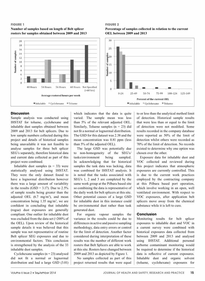
Figure 1 illustrates the number of samples obtained from 2009 until 2013

and the belt splicer roster length. Figure 2 shows the number of historical and current samples for belt splicers in relation to a percent of the current OEL.

Table 4 details the IHSTAT outputs for inhalable dust, toluene, cyclohexane and other agents in comparison to the current OEL.

Statistical analysis showed that inhalable dust samples (n = 33) were the only dataset found to have a lognormal distribution. Despite a wide GSD (3.17), confidence in this data and the conclusions with regard to potential exposures is possible because of the number of samples obtained, a low mean sample concentration of 1.35 mg/m3 and only 2.5% of samples were above the adjusted OEL (6.7 mg/m3). Mean sample concentration was approximately 20% of the adjusted OEL and the UCL95 was 2.31 mg/m3 which is less than 50% of the adjusted OEL.

Cyclohexane sample analysis (n = 23) did not fit a normal or lognormal distribution. The GSD was 3.01. The sample mean was 1.17 ppm, less than 5% of the adjusted OEL (50 ppm).

Toluene sample analysis (n = 23) also did not fit a normal or lognormal distribution. The GSD was 2.38 and the mean concentration was 0.81 ppm, less than 5% of the adjusted OEL (25 ppm).

TABLE 3Comparison of current exposure standard, TWA and/or STEL (equivalents)(Source: Safe Work Australia, 2011; Health & Safety Executive (HSE), 2005; American Conference of Industrial Hygienists (ACGIH), 2013; National Institute for Occupational Safety and Health (NIOSH), 2010a, 2010b, 2010c; Occupational Safety and Health Administration (OSHA), 2006a, 2006b, 2006c, 2012a, 2012b).

Jurisdiction Rogue (inhalable) dust

Cyclohexane (TWA)

Cyclohexane (STEL)

Toluene (TWA)

Toluene (STEL)

Safe Work Australia OEL 10 mg/m3 100 ppm 300 ppm 50 ppm 150 ppm

HSE UK EH40 Workplace Exposure Limit (WEL)

10 mg/m3 100 ppm 300 ppm 50 ppm 100 ppm

ACGIH Threshold Limit Values (TLV)

10 mg/m3 100 ppm - 20 ppm -

NIOSH Recommended Exposure Limit (REL)

Not established (Iron oxide= 5mg/ m3)

300 ppm - 100 ppm

150 ppm

OSHA Permissible Exposure Limit (PEL)

15 mg/m3 300 ppm - 200 ppm

300 ppm

TABLE 4Summary of belt splicer exposure results (current and historical data combined) from IHSTAT analysis

Key Agents Number of samples

Mean Geometric Standard Deviation (GSD)

OEL (TWA, 8hr)

Reduction factor

Adjusted OEL (TWA, 12 hr)

Distribution fit (LogNormal, Normal, Both, Neither)

95th percentile Upper Confidence Limit (UCL95)

Mean Variance Unbiased Estimate (MVUE)

Percent of samples above the adjusted OEL (%)

Inhalable dust (rogue) (mg/m3) 33 1.353 3.173 10 0.67 (a) 6.7 LogNormal 2.309 1.326 2.5

Cyclohexane (ppm) 23 1.170 3.012 100 0.5 (b) 50 Neither N/A N/A 0

Toluene (ppm) 23 0.809 2.384 50 0.5 (b) 25 Neither N/A N/A 0

Other agents

Methylcyclohexane (ppm) 23 0.270 1.831 400 0.5 (b) 200 Neither N/A N/A 0

n-Heptane (ppm) 23 0.260 1.778 400 0.5 (b) 200 Neither N/A N/A 0

n-Hexane (ppm) 20 0.284 1.982 20 0.5 (b) 10 Neither N/A N/A 0

(a) reduction factor calculated for inhalable dust by the following formula: 170hr / x (where x is the average number of hours worked in a month)(b) reduction factor calculated for volatile organic solvents using brief and scala model

Volume 6 Issue 2 • September 2014 JOURNAL OF HEALTH AND SAFETY, RESEARCH AND PRACTICE 15

DiscussionSample analysis was conducted using IHSTAT for toluene, cyclohexane and inhalable dust samples obtained between 2009 and 2013 for belt splicers. Due to low sample numbers collected during this project and details of historical samples being unavailable it was not feasible to analyse samples for three belt splicer SEG’s separately, therefore historical data and current data collected as part of this project were combined.

Inhalable dust samples (n = 33) were statistically analysed using IHSTAT. They were the only dataset found to have a lognormal distribution however there was a large amount of variability in the results (GSD = 3.17). Due to 2.5% of sample results being greater than the adjusted OEL (6.7 mg/m3), and mean concentration being 1.35 mg/m3, we are confident in concluding that inhalable (rogue) dust exposures are generally compliant. One outlier for inhalable dust was excluded from the data set (>200% of the OEL). Upon review of the historical sample details it was believed that this sample was not representative of routine Belt splicer SEG exposures and due to environmental factors. This conclusion is strengthened by the analysis of the 33 inhalable dust samples.

Cyclohexane samples (n = 23) analysed did not fit a normal or lognormal distribution and had a large GSD (3.01)

which indicates that the data is quite varied. The sample mean was less than 5% of the relevant adjusted OEL. Similarly, Toluene samples (n = 23) did not fit a normal or lognormal distribution. The GSD for this dataset was 2.38 and the mean concentration was 0.81 ppm (less than 5% of the adjusted OEL).

The large GSD was potentially due to non-homogeneity of the SEG’s/tasks/environment being sampled. In acknowledging that for historical samples the task data was lacking, data was combined for IHSTAT analysis. It is noted that the tasks associated with SEG’s 1, 2 and 3 are completed by the same work group at the Pilbara based site so combining the data is representative of the daily work for belt splicers at this site. Other potential causes of a large GSD for inhalable dust in this instance could be environmental dust rather than task generated dust.

For organic vapour samples the variance in the results could be due to differences in active and passive sampling methodology, data entry errors or control for the limit of detection. Another factor considered during interpretation of these results was the number of different work rosters that Belt Splicers are able to work at this site. Rosters have changed between 2009 and 2013 as depicted by Figure 1.

No samples collected as part of this project returned results that were equal

to or less than the analytical method limit of detection. Historical sample results that were less than or equal to the limit of detection were not modified. Some results recorded in the company database were reported as 50% of the limit of detection whilst others were recorded as 70% of the limit of detection. No records existed to determine why one option was chosen over the other.

Exposure data for inhalable dust and VOC collected and reviewed during this project indicates that atmospheric exposures are currently controlled. This is due to the current work practices employed by the contracting company at this Pilbara based port operation, which involve working in an open, well ventilated environment. With respect to VOC exposures, after application belt splicers move away from the chemical substance while it is left to cure.

ConclusionMonitoring results for belt splicer exposures to inhalable dust and VOC in a current survey were combined with historical exposures data collected from between 2009 and 2013 and analysed using IHSTAT. Additional personal airborne contaminant monitoring would be required to determine if the historical data is reflective of current exposures. Inhalable dust and organic solvent (toluene, cyclohexane) exposures for

FIGURE 1Number of samples based on length of Belt splicer rosters for samples obtained between 2009 and 2013

FIGURE 2Percentage of samples collected in relation to the current OEL between 2009 and 2013

16 JOURNAL OF HEALTH AND SAFETY, RESEARCH AND PRACTICE Volume 6 Issue 2 • September 2014

belt splicers at the site appear adequately controlled when compared to the current OELs, suitably adjusted to reflect typical work shift rosters. The results indicate that current work practices including working in an open, well ventilated environment and moving away from chemicals while curing are sufficient and appropriate. However, training for the belt splicers on the health hazards, routes of entry and risk controls associated with the chemical substances used would be beneficial.

This paper was first presented to the 31st AIOH annual conference Sydney 30 November- 4 December 2013

ReferencesAgnew, J. (1986). Neurotoxicity of organic

solvents. American Association of Occupational Health Nurses Journal. 34(11), 539-542

American Conference of Industrial Hygienists (ACGIH). (2013). TLVs and BEIs: ACGIH, Cincinnati, US

Banerjee, K.K., Wang, H. & Pisaniello, D. (2006). Iron-Ore Dust and its Health Impacts. Environmental Health, 1(6), 11-16

Benignus, V.A, Bushnell, P.J., Boyes, W.K., Eklund, C. & Kenyon, E.M. (2009). Neurobehavioral Effects of Acute Exposure to Four Solvents: Meta-analyses. Toxicological Sciences. 109(2), 296-305

Borak, J., Slade, M.D. & Russi, M. (2005). Risks of brain tumors in rubber workers: a metaanalysis. Journal of Environmental Medicine. 47, 294-298

Chen, R., Dick, F., Semple, S., Seaton, A. & Walker, L.G. (2001). Exposure to organic solvents and personality. Occupational and Environmental Medicine. 58, 14-18

Cherrie, J.W., Howie, R. & Semple, S. (2010). Monitoring for Health Hazards at Work.(4th Ed.) Blackwell Publishing, Chichester UK.

Creely, K.S., Hughson, G.W., Cocker, J. & Jones, K. (2006). Assessing isocyanate exposures in polyurethane industry sectors using biological and air monitoring methods. Annals of Occupational Hygiene. 50(6), 609-621

DeVocht, F., Straif, K., Szeszenia-Dabrowska, N., Hagmar, L., Sorhan, T., Burstyn, I., Vermeulen, R. & Kromhout, H. (2005). A database of exposures in the rubber manufacturing industry: design and quality control. Annals of Occupational Hygiene. 49(8), 691-701

Department of Health, Western Australia. (2010). Impact of dust on Port Hedland. Retrieved from: http://www.public.health.

wa.gov.au/cproot/2915/2/Western%20Australian%20Department%20of%20Health%20-%20Impact%20of%20Dust%20on%20Port%20Hedland.pdf

Department of Minerals & Energy. (1999). Adjustment of exposure standards for extended workshifts – guideline. Retrieved from: http://www.dmp.wa.gov.au/documents/Guidelines/MSH_G_AdjustmentOfExposureStandardsForExtendedWorkshifts.pdf

Department of Mines & Petroleum. (2010). Management of fibrous minerals in Western Australian mining operations – guideline: Resources Safety, Department of Mines and Petroleum (Western Australia), 1-5

Dost, A.A., Redman, D. & Cox, G. (2000). Exposure to rubber fume and rubber process dust in the general rubber goods, tyre manufacturing and retread industries. Annals of Occupational Hygiene. 44(5), 329-342

Durmusoglu, E., Aslan, S., Can, E. & Bulut, Z. (2007). Health risk assessment of worker’ exposure to organic compounds in a tire factory. Human and Ecological Risk Assessment. 13(1), 209-222

Echeverria, D., Fine, L., Langolf, G., Schork, A. & Sampaio, C. (1989). Acute neurobehavioural effects of toluene. British Journal of Industrial Medicine. 46, 483-495

Filley, C.M., Halliday, W. & Kleinschmidt-DeMasters, B.K. (2004). The effects of toluene on the central nervous system. Journal of Neuropathology and Experimental Neurology. 63(1), 1-12

Foo, S.C., Jeyartnam, J. & Koh, D. (1990). Chronic neurobehavioural effects of toluene. British Journal of Industrial Medicine. 47, 480-484

Gardiner, K., & Harrington, J.M. (2005). Occupational Hygiene (3rd ed.) Massachusetts, Blackwell Publishing.

Health & Safety Executive. (2005). HSE UK EH40 Workplace Exposure Limit. Retrieved from: http://www.hse.gov.uk/pubns/books/eh40.htm

International Agency for Research on Cancer (IARC). (2013). Agents classified by the IARC Monographs, volumes 1-107. Retrieved from: http://monographs.iarc.fr/ENG/Classification/ClassificationsAlphaOrder.pdf

International Agency for Research on Cancer (IARC). (2012). Occupational Exposures in the Rubber-manufacturing Industry. Retrieved from: http://monographs.iarc.fr/ENG/Monographs/vol100F/mono100F-36.pdf

Lynge, E., Anttila, A. & Hemminki, K. (1997). Organic solvents and cancer. Cancer Causes and Control. 8, 406-419

Malaguarnera, G., Cataudella, E., Giordano, M., Nunnari, G., Chisari, G. & Malaguarnera, M. (2012). Toxic hepatitis in occupational exposure to solvents. World Journal of Gastroenterology. 18(22), 2756-2766

Meijer, E., Heederik, D. & Kromhout, H. (1998). Pulmonary effects of inhaled dust and fumes: exposure-response study in rubber workers. American Journal of Industrial Medicine. 33, 16-23

Mulhausen, J.R. & Damiano, J. (1998). A Strategy for Assessing and Managing Occupational Exposures (2nd Ed.) Fairfax USA, AIHA Press.

National Institute for Occupational Safety and Health (NIOSH). (2010a). NIOSH Pocket Guide to Chemical Hazards: Cyclohexane. Retrieved from: http://www.cdc.gov/niosh/npg/npgd0163.html

National Institute for Occupational Safety and Health (NIOSH). (2010b). NIOSH Pocket Guide to Chemical Hazards: Iron Oxide dust and fume. Retrieved from: http://www.cdc.gov/niosh/npg/npgd0344.html

National Institute for Occupational Safety and Health (NIOSH). (2010c). NIOSH Pocket Guide to Chemical Hazards: Toluene. Retrieved from: http://www.cdc.gov/niosh/npg/npgd0619.html

Occupational Safety and Health Administration (OSHA). (1998). Method 111 Toluene. Retrieved from: http://www.osha.gov/dts/sltc/methods/organic/org111/org111.html

Occupational Safety and Health Administration (OSHA). (2000). Method 07 Organic Vapours. Retrieved from: http://www.osha.gov/dts/sltc/methods/organic/org007/org007.html

Occupational Safety and Health Administration (OSHA). (2006a). Rouge (Total Dust). Retrieved from: https://www.osha.gov/dts/chemicalsampling/data/CH_266300.html

Occupational Safety and Health Administration (OSHA). (2006b). Table Z-1 Limits for Air Contaminants. Retrieved from: https://www.osha.gov/pls/oshaweb/owadisp.show_document?p_table=STANDARDS&p_id=9992

Occupational Safety and Health Administration (OSHA). (2006c). Table Z-2 Limits for Air Contaminants. Retrieved from: https://www.osha.gov/pls/oshaweb/owadisp.show_document?p_table=STANDARDS&p_id=9993

Occupational Safety and Health Administration (OSHA). (2012a). Cyclohexane. Retrieved from: https://www.osha.gov/dts/chemicalsampling/data/CH_230600.html

Volume 6 Issue 2 • September 2014 JOURNAL OF HEALTH AND SAFETY, RESEARCH AND PRACTICE 17

Occupational Safety and Health Administration (OSHA). (2012b). Particulates Not Otherwise Regulated (Total Dust). Retrieved from: https://www.osha.gov/dts/chemicalsampling/data/CH_259640.html

Perico, A., Cassinelli, C., Brugnone, F., Bavazzano, P., & Perbellini, L. (1999). Biological monitoring of occupational exposure to cyclohexane by urinary 1,2- and 1,4-cycloheanediol determination. International Archives of Occupational and Environmental Health. 72, 115-120

Pickford, G., & Davies, B. (2007). Chapter 5 Aerosols. In: C. Tillman (Ed), Principles of Occupational Health & Hygiene: An Introduction. Allen & Unwin, NSW.

Safe Work Australia (2011). Workplace Exposure Standards for Airborne Contaminants. Retrieved from: http://www.safeworkaustralia.gov.au/sites/SWA/about/Publications/Documents/639/Workplace_Exposure_Standards_for_Airborne_Contaminants.pdf

Safe Work Australia (2013). Guidance on the Interpretation of Workplace Exposure Standards for Airborne Contaminants. Retrieved from: http://www.safeworkaustralia.gov.au/sites/swa/about/publications/pages/workplace-exposure-standards-airborne-contaminants

Standards Australia. (2003). Workplace air quality - Sampling and analysis of volatile organic compounds by solvent desorption/gas chromatography - Diffusive sampling method (AS2986.2-2003). Retrieved from http://www.standards.org.au/

Standards Australia. (2009). Workplace atmospheres – Method for sampling and gravimetric determination of inhalable dust (AS/NZS3640-2009). Retrieved from http://www.standards.org.au/

Vermeulen, R., Talaska, G., Schumann, B., Bos, R.P., Rothman, N. & Kromhout, H. (2002). Urothelial cell DNA adducts in rubber workers. Environmental and Molecular Mutagenesis. 39, 306-313

Yuasa, J., Kishi, R., Eguchi, T., Harabuchi, I., Kawai, T., Ikeda, M., Sugimoto, R. & Miyake, H. (1996). Investigation on neurotoxicity of occupational exposure to cyclohexane: a neurophysiological study. Occupational and Environmental Medicine. 53, 174-179

18 JOURNAL OF HEALTH AND SAFETY, RESEARCH AND PRACTICE Volume 6 Issue 2 • September 2014

Stretching but not too far: Understanding adaptive behaviour using a model of organisational elasticityStephen Cowley1 and David Borys2

AbstractThis paper describes a model of organisational elasticity that conveys an image of work and hazards as inextricably linked and maintained under control through safe-place measures. It draws on systems theory and moves beyond linear views of accident causation to depict workplace system failures as emergent rather than resultant properties of the system. The model applies to work and safety and is based on the recognition that people “at the blunt end” who design the systems and processes used in organisations make a number of assumptions about the reality of life for people at the work face, “at the sharp end”. Generally there is a gap between work as imagined (at the blunt end) and work as actually done (at the sharp end). In such systems, human performance must be variable and it is the variability that is both the reason for successful operation of workplaces and sometimes the reason for accidents. Therefore, failures cannot be prevented by eliminating performance variability. Instead risk and safety analyses should try to understand the nature of variability of normal performance and distinguish between drift that is adaptive and improves organisational performance and drift that exposes people to risk. The drift can be conceptualised as elasticity in the system and when the limits of elasticity are reached there is exposure to risk. Thus the elasticity model can be used to illustrate both the need for and the implications of adaption and highlights that people need to be able to correctly anticipate risks before failures and harm occur.

CITE THIS ARTICLE ASCowley, S. & Borys, D., (2014), Stretching but not too far: Understanding adaptive behaviour using a model of organisational elasticity, J Health & Safety Research & Practice 6(2), 18-22

KEY WORDS Elasticity; drift; adaption; variability, resilience, high-reliability, safety management

CORRESPONDENCEStephen CowleyEmail: info@safeworksolutions.co.uk

1 SafeWork Solutions Ltd2 School of Applied Science, RMIT University,

Melbourne, Australia

IntroductionIt has been argued that the discipline of occupational health and safety (OHS) has developed and evolved through a technical age, a human factors age and a management systems age. (Hale and Hovden, 1998). Through these periods various models of accident causation have been used to explain the phenomenon.

Perhaps one of the most recognisable models that persisted through and beyond the technical age was that of Heinrich (1959). He used dominoes stood on edge to illustrate a linear culmination of a series of events or circumstances which occur in a specific and recognisable order (Hollnagel, 2004).

OHS developed through the management systems age and it has been since been argued that we have entered an “integration age” (Glendon et al., 2006) where previous ways of thinking are not lost, but remain available to be reflected upon as multiple and more complex perspectives develop

and evolve. Consequently we have looked to systems theory to understand and help us think about managing OHS in organisations and have drawn upon James Reason’s work and his familiar “Swiss Cheese model” (Reason, 1995).

Hollnagel (2004) sees this model - and others such as root cause analysis and fault tree analysis - as linear, sequential models that seek causation through a retracing of sequential steps that led to an event; therefore the models are temporal. However, he suggests that temporal order does not equate to causality; prediction of future events cannot rely on the order of two or more preceding events in a sequence. He argues that, in the context of increasingly complex socio-technical systems, a systemic model is required.

In these complex systems Hollnagel suggests that human performance is variable and approximate and it is the variability that is the main reason for accidents. Thus accidents are an emergent property of complex socio-technical systems; they “emerge from combinations of normal variability…” (Hollnagel, 2007). He stresses, however, that this variability is not the same as human error. On the contrary; the variability is necessary for the proper functioning of the system. The variability is deliberate and purposeful and comes from the need to be adaptive in a constructive manner. The system demands the variability because it is changing over time. Consequently Borys et al (2009) have proposed that we are moving into a fifth age of safety, the ‘adaptive age’; an age which transcends rather than replaces the other ages of safety. This requires that we move beyond linear views of accident causation and find a depiction of workplace risk control that more satisfactorily shows how accidents are emergent rather than resultant properties of the system. A system is defined here as “a concept of a recognizable whole consisting of a number of parts which interact in an organized way” (Waring, 1996, p 6).

Hollnagel (2004, p 44) suggested, “We cannot think about something without having the words and concepts to describe it, or without having some frame of reference” and Dekker (2006, p 81) subse-quently wrote, “An accident model is a

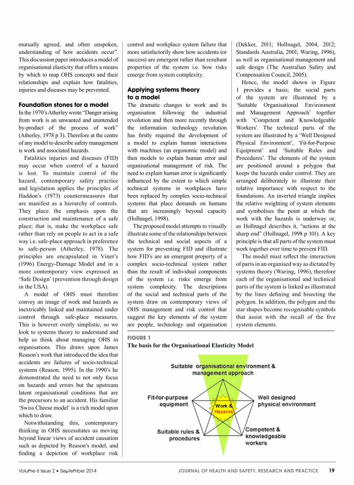
Volume 6 Issue 2 • September 2014 JOURNAL OF HEALTH AND SAFETY, RESEARCH AND PRACTICE 19

mutually agreed, and often unspoken, understanding of how accidents occur”. This discussion paper introduces a model of organisational elasticity that offers a means by which to map OHS concepts and their relationships and explain how fatalities, injuries and diseases may be prevented.

Foundation stones for a modelIn the 1970’s Atherley wrote “Danger arising from work is an unwanted and unintended by-product of the process of work” (Atherley, 1978 p 3). Therefore at the centre of any model to describe safety management is work and associated hazards.

Fatalities injuries and diseases (FID) may occur when control of a hazard is lost. To maintain control of the hazard, contemporary safety practice and legislation applies the principles of Haddon’s (1973) countermeasures that are manifest as a hierarchy of controls. They place the emphasis upon the construction and maintenance of a safe place; that is, make the workplace safe rather than rely on people to act in a safe way i.e. safe-place approach in preference to safe-person (Atherley, 1978). The principles are encapsulated in Viner’s (1996) Energy-Damage Model and in a more contemporary view expressed as ‘Safe Design’ (prevention through design in the USA).

A model of OHS must therefore convey an image of work and hazards as inextricably linked and maintained under control through safe-place measures. This is however overly simplistic, so we look to systems theory to understand and help us think about managing OHS in organisations. This draws upon James Reason’s work that introduced the idea that accidents are failures of socio-technical systems (Reason, 1995). In the 1990’s he demonstrated the need to not only focus on hazards and errors but the upstream latent organisational conditions that are the precursors to an accident. His familiar ‘Swiss Cheese model’ is a rich model upon which to draw.

Notwithstanding this, contemporary thinking in OHS necessitates us moving beyond linear views of accident causation such as depicted by Reason’s model, and finding a depiction of workplace risk

control and workplace system failure that more satisfactorily show how accidents (or success) are emergent rather than resultant properties of the system i.e. how risks emerge from system complexity.

Applying systems theory to a modelThe dramatic changes to work and its organisation following the industrial revolution and then more recently through the information technology revolution has firstly required the development of a model to explain human interactions with machines (an ergonomic model) and then models to explain human error and organisational management of risk. The need to explain human error is significantly influenced by the extent to which simple technical systems in workplaces have been replaced by complex socio-technical systems that place demands on humans that are increasingly beyond capacity (Hollnagel, 1998).

The proposed model attempts to visually illustrate some of the relationships between the technical and social aspects of a system for preventing FID and illustrate how FID’s are an emergent property of a complex socio-technical system rather than the result of individual components of the system i.e. risks emerge from system complexity. The descriptions of the social and technical parts of the system draw on contemporary views of OHS management and risk control that suggest the key elements of the system are people, technology and organisation

(Dekker, 2011; Hollnagel, 2004, 2012; Standards Australia, 2001; Waring, 1996), as well as organisational management and safe design (The Australian Safety and Compensation Council, 2005).

Hence, the model shown in Figure 1 provides a basis; the social parts of the system are illustrated by a ‘Suitable Organisational Environment and Management App roach’ together with ‘Competent and Knowledgeable Workers’. The technical parts of the system are illustrated by a ‘Well Designed Physical Environment’, ‘Fit-for-Purpose Equipment’ and ‘Suitable Rules and Procedures’. The elements of the system are positioned around a polygon that keeps the hazards under control. They are arranged deliberately to illustrate their relative importance with respect to the foundations. An inverted triangle implies the relative weighting of system elements and symbolises the point at which the work with the hazards is underway or, as Hollnagel describes it, “actions at the sharp end” (Hollnagel, 1998 p 101). A key principle is that all parts of the system must work together over time to prevent FID.

The model must reflect the interaction of parts in an organised way as dictated by systems theory (Waring, 1996), therefore each of the organisational and technical parts of the system is linked as illustrated by the lines defining and bisecting the polygon. In addition, the polygon and the star shapes become recognisable symbols that assist with the recall of the five system elements.

FIGURE 1 The basis for the Organisational Elasticity Model

20 JOURNAL OF HEALTH AND SAFETY, RESEARCH AND PRACTICE Volume 6 Issue 2 • September 2014

Just as a key principle of the model is that all parts of the system must work together over time to prevent FID, the converse is also true. Different parts of the system can degrade and the conjunction of these degradations over time and under the right circumstances could lead to FID. However, the model at this basic level is relatively static and does not reflect how we see the evolution of safety beyond the simple application of an OHS management system. Thus the model has been developed to address the needs of an ‘adaptive age’ (Borys et al., 2009).

A systems model in an adaptive ageThe concept of an adaptive age is based on the recognition that people ‘at the blunt end’ who design the systems and processes used in organisations make a number of assumptions about the reality of life for people at the work face, ‘at the sharp end’ (Hollnagel, 1998). Generally those people at the sharp end will have to make compromises to meet process demands in ways that are not anticipated and often not understood by the people at the blunt end. For example, a production worker adding a powder ingredient to a tank of liquid may find that moisture has entered the bags of powder and the resultant lumps will have to be broken before addition to ensure steady reaction and prevent spattering. Alternatively the worker may find that the tank temperature has been increased for downstream process reasons and steam now moistens the neck of the bag. In both cases the routine process for adding the powder must be varied. In such systems human perfor mance must be variable and approx imate and it is the variability that is both the reason for successful operation of workplaces but also, in some cases, accidents. Hence accidents (hazards) are an emergent property of complex socio-technical systems; they “…emerge from combinations of normal variability…” (Hollnagel, 2007). This variability how-ever, is not the same as human error. On the contrary, performance variability is necessary for normal functioning in work places.

Variability is deliberate and purposeful and comes from the need to be adaptive

in a constructive manner as outlined in the powder and tank example above. The system requires the variability because it is changing over time. Given the many sub-systems, there is likely to be variability on several time scales simultaneously. For example, process and production fluctuations demand variability within short time frames of seconds or minutes; working environment changes occur over hours or days and organisational changes happen quite slowly.

On finding that procedures are being varied, organisations and managers within those organisations will usually attempt to limit actions through the re-writing of procedures to restrict the range of permitted actions. Eventually the procedures (rules) may become so restrictive that the work can no longer be completed efficiently or productively by following the procedures (Hale and Borys, 2013a, b).

The reasons the workers vary the pro-cedures in such cases, however, is generally for reasons of efficiency. However, there must be trade-offs and Hollnagel refers to this as efficiency-thoroughness trade-offs (ETTO)(Hollnagel, 2009), i.e. on the one hand people genuinely try to do what they are supposed to do and be as thorough as necessary while on the other hand they try to be as efficient as possible.

In order to find and take short cuts such that things may be done more efficiently it is necessary to make assumptions based on expectations. This is assisted by regularity in the work environment. So, if condition A is always true in situation B, then there is no need to check for the condition; if two different formulations of powder are used in a production process and each is stored in bags in an allotted space the production worker is likely to collect a bag without checking the label, instead relying on the stores person to have correctly placed the materials.

Such variability must be considered with respect to the context within which the system operates. The context is influenced both externally (legislation, public policy, eco nomics, standards, technology, indust-rial relations) and internally (business policy & goals, production schedules, organisational structure, decision making, technology adopted, resources,

organisational history, power relations, risk perception, safety culture) (Waring, 1996).

A key element of the context is the organisational structure, management and culture. In this regard recent research into the reasons for success (low number of serious mishaps) of complex organisations (socio-technical systems) has focussed attention on mindful leadership. Such organisations have been referred to as High Reliability Organisations (HRO) and are characterised by “collective mindfulness” which means, among other things, man-agers are constantly worried about the possibility of failure, they are reluctant to draw quick conclusions and always look for more evidence and they are sensitive to the experience of people at the sharp end and encourage them to speak up. Mindful organisations exhibit “chronic unease” and are aware that despite normal functioning, danger is lurking below the surface. They are able to detect warnings especially from weak signals and they respond strongly to them; they detect variability and respond to it appropriately (Weick and Sutcliffe, 2007).

However, failures cannot be prevented by eliminating performance variability. Instead risk and safety analyses should try to understand the nature of variability of normal performance and use that to identify conditions that may lead to both positive and adverse outcomes. The proposed adaptive age requires an acceptance by organisational leaders that groups of workers may, through interaction with one another and the tasks they perform together, in the context of the socio-technical system, create their own shared meanings about what it is to work safely. For example, at an airport the apron was declared a mandatory hearing protection area. While driving a catering truck the driver and co-driver were not exposed to excessive noise and hearing protection interfered with warnings that drivers rely upon for safe driving. The drivers considered the situation and consciously varied and contravened the procedure by donning the protective equipment only before alighting from the vehicle at the aircraft.

In some organisations (systems) adapting may be a pre-requisite for safe performance whilst in others it may be disastrous. The adaptive age does not suggest a free-for-

Volume 6 Issue 2 • September 2014 JOURNAL OF HEALTH AND SAFETY, RESEARCH AND PRACTICE 21

all so much as embodying the capacity to be adaptive rather than rule-bound. This involves providing people at the sharp end with the skills of knowing when adaptation is good for safety and when it could influence FID. In a mindful organisation, the airline catering truck drivers’ adaption will be identified and rather than apply punitive measures the variation will be assessed and discussed and if appropriate the procedures amended.

The design of processes and the writing of procedures (at the blunt end) for implementation that requires variability and adaptability at the sharp end, often results in a gap between work as imagined (at the blunt end) and work as actually done (at the sharp end) (Dekker and Suparamaniam, 2005; Hollnagel et al., 2006). This is referred to as “drift”. The adaptive age requires that people at all levels of the organisation are be able to distinguish between drift that is adaptive and improves organisational performance and drift that exposes people to risk. People need to be able to correctly anticipate risks before failures and harm occur.

For example, operation of a commercial fishing vessel demands high levels of adaptability; in particular, the location of the fishing (e.g. in-shore versus deep sea) and the weather necessitates variability in the work. The use of personal flotation devices (PFDs) while working at sea is important but under some circumstances use may not be necessary or appropriate; when the weather is fair and the sea calm the PFD may be an unnecessary hindrance and when casting nets or pots it could lead to snagging and the fisher being dragged overboard. Therefore the fishers need to decide when PFDs should be donned (Cowley, 2006).

The answer is neither simple nor generic. For example, simply requiring PFDs to be worn when the sea is rough is not appropriate because the extent to which wave height and wind will affect a vessel is dependent upon vessel type and size. Hence skippers and fishers decide the criteria for PFD use based upon their knowledge of their vessel, their fishing practices and their experience of the sea.

A free-for-all is not desirable so the skipper, being the workplace manager, documents within the vessel safety management plan the criteria that define what is considered rough and practices that may be negatively influenced by a PFD. Thus boundaries are set that enable the skipper to monitor work practice and observe the extent to which there is acceptable variability.

So, on the basis of these principles, we are able to develop the elasticity model as shown in Figure 2. The model illustrates the boundary of the area within which variability is acceptable. When variability leads to drift, the concentric rings indicate where warnings may be detected before drifting into failure. Variability that drifts towards failure can occur within each of the system elements and thus one may picture the polygon as an elastic frame that may be stretched in five directions corresponding to the system elements. The degree to which the polygon is stretched is dependent upon the degree of variability as illustrated in Figure 2. Variability within the boundary of optimal performance means that the drifting (stretching) does not extend into the warnings zone1.

The illustration of the elasticity model suggests a stretching of the polygon in one direction. However, the nature of a system such as being discussed is that stretching in one direction will result in deformation

of the whole. As Hollnagel (2011, p 15) suggests “accidents result from unexpected combinations (resonance) of normal performance variability”.

As previously discussed, the solution to drift is not to further restrict performance variability. Rather, it is more appropriate to monitor and detect drift toward failure. Such drift may be detected by warnings (Hopkins, 2007). These warnings are traditionally considered to be in the form of near misses and process interruptions and will occur once drift into the warnings zone has occurred. More contemporary views suggest that there should be a focus on weak signals that indicate that drift is occurring and that a strong response is required before there are near misses and injuries (Dekker, 2011; Hollnagel, 2008; Hollnagel et al., 2011; Hopkins, 2008; Weick and Sutcliffe, 2007). These signals must be conveyed to the organisational management level through conversations with people at the blunt end, through audits, production data, etc.

Of course, variability is an efficiency-thoroughness trade-off and therefore variability in actions is a component of performance. Hence the boundary between the zone of acceptable variability and the warnings zone is, in reality, a boundary between optimal and sub-optimal performance.

FIGURE 2 A model of organisational elasticity

1. The inner circle representing the area of optimal perormance is coloured green, the warnings zone amber and the failure zone red.

22 JOURNAL OF HEALTH AND SAFETY, RESEARCH AND PRACTICE Volume 6 Issue 2 • September 2014

In a socio-technical environment where we know that variability is not only natural but necessary for successful performance, conceiving safety as a reduced number of adverse events will not help us. This will lead us to the conclusion that negative outcomes are caused by failures and we will try to eliminate failures which in themselves are unpredictable and rare. Instead we need to conceive safety as the ability to succeed under varying conditions and, as Hollnagel puts it, “Improve resilience” (Hollnagel, 2008). Thus recognising drift and warnings and acting on these will improve resilience. As Hollnagel suggests, “ways in which things go right are special cases of the ways in which things go wrong.” Therefore, the best way to improve system safety is to study how things go right, and to generalise from that (Hollnagel, 2008); we study every day, normal work and actions within the zone of optimal variability i.e. the inner zone in the Organisational Elasticity Model. We want to encourage and amplify the optimal variability and damp sub-optimal variability. This requires us to study work as done rather than imagined and understand variability. In accord with High Reliability Organisation (HRO) theory we need to be mindful of warnings, that is detect drift from the zone of optimal variability into the warning zone and respond strongly to this before the drift extends into the zone of failure i.e. there must be a strong response to weak signals.

ConclusionThe adaptive age embraces both adaptive practices and resilience engineering and requires a change in perspective from one that views human variability as a liability and in need of control, to one that views human variability as a asset and important for safety. Embracing variability as an asset challenges current thinking about occupational health and safety.

The gap between work as imagined and work as done and the failure of OHS management systems and safety rules to adequately control risk mean that a new perspective is required.

The Organisational Elasticity Model offers a systemic model by which to map OHS concepts and their relationships and explain how prevention and analysis of

fatalities, injuries and diseases may be illustrated in the real world. The model uses a polygon and star as recognisable symbols that may be readily recalled and used as a lens through which to view successful organisational OHS management as well as organisational failure. It may be used to explain the positive as well as the negative elements of variability and explain organisational adaptability.

As such the model encourages people to move away from the notion that rules and rule-compliance are essential to safety; instead the challenge is to accept and encourage informed variability while adopting measures that will enable the detection of weak signals of drift toward failure.

References Atherley, G.R.C., 1978. Occupational Health and

Safety Concepts - Chemical and Processing Hazards. Applied Science Publishers Ltd, London.

Borys, D., Else, D., Leggett, S., 2009. The fifth age of safety: the adaptive age? J Health & Safety Research & Practice 1, 19-27.

Cowley, S., 2006. OH&S in Small Business: Influencing the Decision Makers. The application of a social marketing model to increase the uptake of OHS risk control measures by small business, VIOSH Aust-ralia. University of Ballarat, Ballarat, p. 358.

Dekker, S., 2006. The Field Guide to Under-standing Human Error. Ashagte, Aldershot.

Dekker, S., 2011. Drift into failure: From hunting broken components to understanding complex systems. Ashgate, Aldershot.

Dekker, S., Suparamaniam, N., 2005. Divergent images of decision making in international disaster reilef work Lund University School of Aviation, Ljungbyhed, Sweden.

Glendon, A.I., Clarke, S.G., McKenna, E.F., 2006. Human safety and risk management, 2nd ed, Boca Raton, FL.

Haddon, W., 1973. Energy damage and the ten countermeasure strategies. Journal of trauma 13, 321-331.

Hale, A., Borys, D., 2013a. Working to rule or working safely? Part 2: The management of safety rules and procedures. Safety Science 55 222-231.

Hale, A., Borys, D., 2013b. Working to rule, or working safely? Part 1: A state of the art review Safety Science 55, 207-221.

Hale, A.R., Hovden, J., 1998. Management and culture: the third age of safety. A review of approaches to organizational aspects of safety, health and environment, In: Feyer, A.M., Williamson, A. (Eds.), Occupational injury: Risk prevention and intervention. Taylor and Francis, London.

Heinrich, H.W., 1959. Industrial Accident Prevention: A Scientific Approach, 4th ed. McGraw-Hill.

Hollnagel, E., 1998. Cognitive Reliability and Error Analysis Method (CREAM). Elsevier, Oxford.

Hollnagel, E., 2004. Barriers and Accident Prevention. Ashgate, Aldershot.

Hollnagel, E., 2007. Human Factors: From Liability to Asset. École nationale supérieure des Mines de Paris, Pôle Cindyniques, Sophia Antipolis, France.

Hollnagel, E., 2008. Resilience Engineering and Safety Assessment. MINES ParisTech — Crisis and Risk Research Centre.

Hollnagel, E., 2009. The ETTO principle. Ashgate, Aldershot.

Hollnagel, E., 2011. Understanding Accidents, or How (Not) to Learn from the Past. University of Southern Denmark, Odense.

Hollnagel, E., 2012. FRAM: The functional resonance analysis method: Modelling complex socio-technical systems. Ashgate, Aldershot

Hollnagel, E., Pariès, J., Woods, D., Wreathall, J., 2011. Resilience engineering in practice: A guidebook. Ashgate, Aldershot.

Hollnagel, E., Woods, D.D., Leveson, N., 2006. Resilience Engineering: Concepts And Precepts. Ashgate.

Hopkins, A., 2007. Lessons from Gretley: Mindful Leadership and the Law. CCH Australia Limited, Sydney.

Hopkins, A., 2008. Failure to Learn the BP Texas City Refinery Disaster. CCH, Sydney.

Reason, J., 1995. A systems approach to organiz-ational error. Ergonomics 38, 1708-1721.

Standards Australia, 2001. Australian Standard AS/NZS 4804:2001 Occupational health and safety management systems: General guidelines on principles, systems and supporting techniques. Standards Australia & Standards New Zealand, Sydney.

The Australian Safety and Compensation Council, 2005. Guideline on Safe Design Principles. The Australian Safety and Compensation Council, Canberra.

Viner, D., 1996. Accident Analysis and Risk Control. Derek Viner Pty Ltd, Melbourne.

Waring, A., 1996. Safety Management Systems Chapman & Hall, London.

Weick, K.E., Sutcliffe, K.M., 2007. Managing the unexpected. Josssey-Bass, San Francisco.

A publication for members of the Safety Institute of Australia Ltd