Journal of Geochemical Exploration 108 (2011) 62–72

Contents lists available at ScienceDirect

Journal of Geochemical Exploration

j ourna l homepage: www.e lsev ie r.com/ locate / jgeoexp

Geostatistical methods to identify and map spatial variations of soil salinity

P. Juan a, J. Mateu a, M.M. Jordan b,⁎, J. Mataix-Solera b, I. Meléndez-Pastor b, J. Navarro-Pedreño b

a Department of Mathematics, Campus Riu Sec. University Jaume I. E-12071. Castellón, Spainb Departamento de Agroquímica y Medio Ambiente, Universidad Miguel Hernández de Elche. E-03202. Elche (Alicante), Spain

⁎ Corresponding author. Fax: +34 966658340.E-mail address: manuel.jordan@umh.es (M.M. Jorda

0375-6742/$ – see front matter © 2010 Elsevier B.V. Adoi:10.1016/j.gexplo.2010.10.003

a b s t r a c t

a r t i c l e i n f o

Article history:Received 29 March 2010Accepted 11 October 2010Available online 15 October 2010

Keywords:Bayesian methodologyElectrical conductivitySpatial Gaussian linear mixed modelHierarchical modellingSodiumSoil salinity

The problemof estimating and predicting spatial distribution of a spatial stochastic process, observed at irregularlocations in space, is considered in this paper. Environmental variables usually show spatial dependencies amongobservations, with lead one to use geostatisticalmethods tomodel the spatial distributions of those observations.This is particularly important in the study of soil properties and their spatial variability. In this study geostatisticaltechniques were used to describe the spatial dependence and to quantify the scale and intensity of spatialvariations of soil properties, which provide the essential spatial information for local estimation. In thiscontribution, we propose a spatial Gaussian linear mixed model that involves (a) a non-parametric term foraccounting deterministic trend due to exogenous variables and (b) a parametric component for defining thepurely spatial random variation due possibly to latent spatial processes. We focus here on the analysis of therelationship between soil electrical conductivity and Na content to identify spatial variations of soil salinity. Thisanalysis can be useful for agricultural and environmental land management.

n).

ll rights reserved.

© 2010 Elsevier B.V. All rights reserved.

1. Introduction

There are two main types of soils salinity: dryland salinity, whichoccur on landnot subject to irrigation; and irrigated land salinity. Bothofthem describe areas where soils contain high levels of salts that canaffect plant productivity and soil organisms (Navarro-Pedreño et al.,1997). Under arid or semi-arid conditions and in regions of poor naturaldrainage, there is a real hazard of salts accumulation in soils. Theprocesses by which soluble salts cause salinity and sodicity in soilsinclude: (i) the application of waters containing salts; (ii) weathering ofprimary and secondaryminerals in soils; (iii) organicmatter decay; (iv)watertable instability. The importance of each of those causes dependson soil type, climate, and agricultural management. Accumulation ofdispersive cations, such as Na, in soil solution and the exchange phase(K, Mg, Ca) affect the physical properties of soil, such as structuralstability, hydraulic conductivity, infiltration rate and erosivity.

Historically, the physical behaviour of salt-affected soils has beendescribed in terms of the combined effects of soil salinity, asmeasured bytheECof a saturationextract, andexchangeable sodiumpercentage (ESP)on flocculation and soil dispersion. Based on this, the U.S. SalinityLaboratory Staff (1954) described a saline soil (ECN4 dS/m; ESPb15) anda saline-alkali soil (ECN4 dS/m; ESPN15). By 1979, the term “alkali”waslisted as obsolete by the Soil Science Society of America (although it is stillused by farm advisors and others), and the word “sodic”was used in itsplace with the definition: “a soil having an ESPN15”. Outside the United

States, theword “alkali” is generally used in a narrower context referringonly to soils with: (i) high sodicity and high pH (ESPN15, pHN8.3) and(ii) containing soluble bicarbonate and carbonate (Na/[Cl+SO4]N1)(Gupta andAbrol, 1990). Theuse of the term “alkali” thus allowspracticaldistinctions between saline, sodic, and alkali soils in terms of soilmanagement (Bhumba and Abrol, 1979; Gupta and Abrol, 1990). In thispaper, “saline” and “sodic” are used as defined by the Soil Science Societyof America, while “alkali” is used as defined above.

There is anumber of factors that influence the vulnerability of sites tosalinization (Oster et al., 1996). These factors include: (i) the position ofa site within a landscape (Manning et al., 2001), and (ii) soil type andrainfall. It has been postulated that the combination of information onthese and other factors allows prediction of sites that are vulnerable tosalinity (Navarro et al., 2001). Data sets consisting of rainfall,topography, soil type, and other relevant spatial information can becompiled into a GIS to determine spatial patterns of salinization, and topredict areas that may be at risk. Spatial variations and interrelationsamong variables related to salinity, such as Na content or EC, arecomplex. Thus, full understanding, estimating and mapping of thespatial characteristics of soil salinity facilitates accurate risk assessment(Florinsky et al., 2000) and remedying of environmental problems.

Most soil properties of scientific interest vary continuously inspace and time, and cannot be practically measured or recordedeverywhere. To represent their spatial variations, values of individualvariables or class types at unsampled locations must be estimatedfrom data of those variables recorded at sample sites. The need toprecisely continuous spatial variations is clear, and geostatistics islargely the relevant theory for addressing that need. It embraces a setof stochastic techniques that take into account both the random and

63P. Juan et al. / Journal of Geochemical Exploration 108 (2011) 62–72

structured nature of spatial variables, the spatial distribution ofsampling sites and the uniqueness of any spatial observation (Journeland Huijbregts, 1978; Goovaerts, 1997).

Spatial statistics is one of the major methodologies of environmentalstatistics, and geostatistical methods are an important part of spatialstatistics with wide applications in environmental surveys (e.g., soilscience). In most cases, soil data can be considered as partial realizationsof a random function (stochastic process) over a region, i.e., a spatiallycontinuousprocess, as characterizedbyCressie (1993). Typically, samplesare taken at a finite set of locations in a region and are used to estimatequantities of interest such as the values of the property of interest atunvisited locations. Data of this kind are often called geostatistical data.

An important tool in geostatistics is kriging, which refers to a leastsquare linear predictor that, under certain stationarity assumptions,requires at least the knowledge of covariance parameters and thefunctional form for the mean of the underlying random function.Kriging does not take uncertainty into account in the prediction, butuses plug-in estimates as if they were true. Bayesian inference, incontrast, provides a way to incorporate parameter uncertainty in theprediction by treating the parameters as random variables andintegrating over the parameter space to obtain the predictivedistribution of any quantity of interest (Feyen et al., 2002).

In this paper, we attempt to combine soil properties using spatialstatistical techniques under amodelling framework that we refer to as aGaussian Spatial Linear Mixed Model (GSLMM). This is a general andflexible class of models for handing spatial variation shown byindividual variables in a particular environment. The use of a Bayesianapproach is also compatible with the GSLMM and, thus, is shown in thepaper. Various geostatistical techniques have been discussed in thestatistical literature. For example, the relationship between universalkriging and cokriging with regression modelling has been discussed byStein and Corsten (1991). A complete derivation of a Bayesian approachto kriging has been discussed by Kitanidis (1986), among others. Inaddition, Curreriro and Lele, 1999 have developed a hierarchicalapproach to spatialmodelling, and they have shownhow that approach

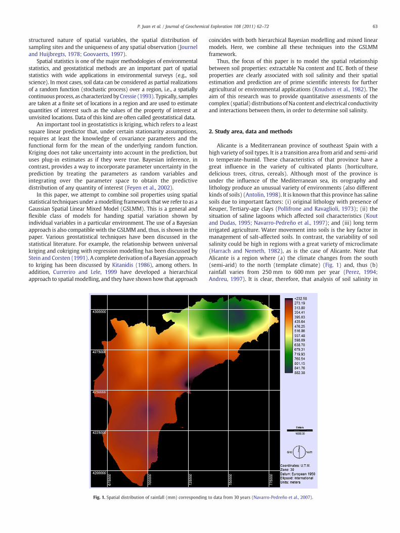
Fig. 1. Spatial distribution of rainfall (mm) corresponding

coincides with both hierarchical Bayesian modelling and mixed linearmodels. Here, we combine all these techniques into the GSLMMframework.

Thus, the focus of this paper is to model the spatial relationshipbetween soil properties: extractable Na content and EC. Both of theseproperties are clearly associated with soil salinity and their spatialestimation and prediction are of prime scientific interests for furtheragricultural or environmental applications (Knudsen et al., 1982). Theaim of this research was to provide quantitative assessments of thecomplex (spatial) distributions of Na content and electrical conductivityand interactions between them, in order to determine soil salinity.

2. Study area, data and methods

Alicante is a Mediterranean province of southeast Spain with ahigh variety of soil types. It is a transition area from arid and semi-aridto temperate-humid. These characteristics of that province have agreat influence in the variety of cultivated plants (horticulture,delicious trees, citrus, cereals). Although most of the province isunder the influence of the Mediterranean sea, its orography andlithology produce an unusual variety of environments (also differentkinds of soils) (Antolin, 1998). It is known that this province has salinesoils due to important factors: (i) original lithology with presence ofKeuper, Tertiary-age clays (Pollifrone and Ravaglioli, 1973); (ii) thesituation of saline lagoons which affected soil characteristics (Koutand Dudas, 1995; Navarro-Pedreño et al., 1997); and (iii) long termirrigated agriculture. Water movement into soils is the key factor inmanagement of salt-affected soils. In contrast, the variability of soilsalinity could be high in regions with a great variety of microclimate(Harrach and Nemeth, 1982), as is the case of Alicante. Note thatAlicante is a region where (a) the climate changes from the south(semi-arid) to the north (template climate) (Fig. 1) and, thus (b)rainfall varies from 250 mm to 600 mm per year (Perez, 1994;Andreu, 1997). It is clear, therefore, that analysis of soil salinity in

to data from 30 years (Navarro-Pedreño et al., 2007).

64 P. Juan et al. / Journal of Geochemical Exploration 108 (2011) 62–72

Alicante is essential for understanding of environmental degradationprocesses in the province.

2.1. Soil sampling and analysis

The Environmental Protection Administration of Alicante provinceinitiated a collaborative research program to establish the presence ofcertain kind of salts in the region. Over 400 hundred soil samples(arable layer) from 46 different agricultural sites (located with GPS)were taken during a period of two years (Fig. 2). Samples were driedat room temperature and EC (1:5 w/v water extraction) andextractable Na content (ammonium acetate 1 M extraction) weredetermined. Soil solution extracts were analysed using atomicabsorption spectrometry to determine the Na concentration.

2.2. Geostatistical theoretical framework

The basic format for univariate geostatistical data is {(ui, z(ui)),i=1,...,n}, where ui identifies a spatial location and z(ui) is a scalarmeasurement taken at location ui. It follows that the basic form of ageostatistical model is a real-valued stochastic process {Z(u): u∈A},which, in turn, is typically considered to be a partial realization of astochastic process {Z(u): u∈ℜ2}. The measurement process Zi can beregarded as a noisy version of an underlying random variable S(ui), thevalue at location ui of a {S(u): u∈ℜ2} that is of prime scientific interest.We call S(u) the signal. The basic model is then extended to one withtwo ingredients: a stochastic process S(u); and a statisticalmodel for themeasurements, Z=(Z1, ..., Zn) conditional on {Z(u): u∈ℜ2}.

The objectives of geostatistical analysis are broadly of two kinds:estimation and prediction. Estimation refers to inference about theparameters of a stochastic model for the data. These may includeparameters of direct scientific interest (e.g., defining a regressionrelationship between a response variable and an exploratory variable,and parameters of indirect interest (e.g., the covariance structure of amodel for S(u)). Prediction refers to inference about the realization of

Fig. 2. The locations of sampling sites

the unobserved signal S(u). Specific prediction objectives mightinclude prediction of the realized value of S(u) at arbitrary location uwithin a region of interest A, or prediction of some property of thecomplete realization of S(u) for all u in A.

Before interpolation and prediction, we need to know thestructure of the spatial variation, and this is done through variogram(or co-variogram) estimation. Several authors have proposed meth-ods for the improvement and robustness of variogram estimation(Cressie and Hawkins, 1980; Cressie, 1993; Curriero and Lele, 1999).To map the spatial variation in soil salinity or to highlight soildegradation by certain salts that are present in the soil, we need toperform spatial predictions. For prediction, we applied our GSLMMmethodology, firstly with matrix X=1 to obtain ordinary kriging(OK) predictions for each variable, and, secondly with X considered ina trend matrix to obtain cokriging and external trend kriging for therelationship between Na content and EC.

After having learned about the co-regionalization model, based onthe experimental cross-variogram and cross-variogram model, we canuse that knowledge of the spatial relations between two or morevariables to predict their values by co-kriging. Typically, the aim is toestimate just one variable, which we may regard as the principal ortarget variable, fromdata of that variables plusdata of oneormore othervariables, which we regard as auxiliary variables. In this sense, the co-kriging is a natural extension of kriging when a multivariate variogramor covariancemodel andmultivariate data are available. Co-kriging andexternal trend krigingmodels are designed for exploiting over-sampledvariables to better estimate under-sampled variables. The classicalmethodology of kriging does not take into account uncertainty inparameter estimation, and this could affect prediction results. Therefore,we used the Bayesian framework to analyze the form of the predictivedistributions for the two soil properties considered in this study.

2.2.1. Gaussian spatial linear mixed models (GSLMM)This section describes a full interactive model that gives an explicit

expression for function f by means of GSLMM. In the GSLMM, it is

(Navarro-Pedreño et al., 2007).

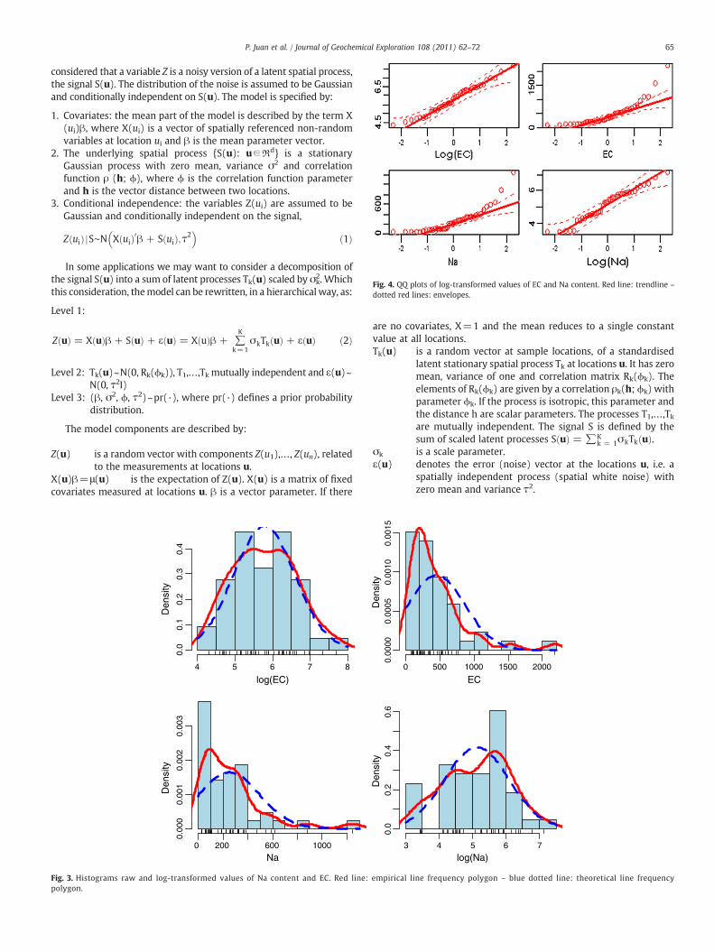
Fig. 4. QQ plots of log-transformed values of EC and Na content. Red line: trendline –

dotted red lines: envelopes.

65P. Juan et al. / Journal of Geochemical Exploration 108 (2011) 62–72

considered that a variable Z is a noisy version of a latent spatial process,the signal S(u). The distribution of the noise is assumed to be Gaussianand conditionally independent on S(u). The model is specified by:

1. Covariates: the mean part of the model is described by the term X(ui)β, where X(ui) is a vector of spatially referenced non-randomvariables at location ui and β is the mean parameter vector.

2. The underlying spatial process {S(u): u∈ℜd} is a stationaryGaussian process with zero mean, variance σ2 and correlationfunction ρ (h; ϕ), where ϕ is the correlation function parameterand h is the vector distance between two locations.

3. Conditional independence: the variables Z(ui) are assumed to beGaussian and conditionally independent on the signal,

ZðuiÞ jS∼N XðuiÞ0β + SðuiÞ;τ2� �

ð1Þ

In some applications we may want to consider a decomposition ofthe signal S(u) into a sum of latent processes Tk(u) scaled by σk

2. Whichthis consideration, themodel can be rewritten, in a hierarchical way, as:

Level 1:

ZðuÞ = XðuÞβ + SðuÞ + εðuÞ = XðuÞβ + ∑K

k=1σkTkðuÞ + εðuÞ ð2Þ

Level 2: Tk(u)~N(0, Rk(ϕk)), T1,…,Tk mutually independent and ε(u)~N(0, τ2I)

Level 3: (β, σ2, ϕ, τ2)~pr(·), where pr(·) defines a prior probabilitydistribution.

The model components are described by:

Z(u) is a random vector with components Z(u1),…, Z(un), relatedto the measurements at locations u.

X(u)β=μ(u) is the expectation of Z(u). X(u) is a matrix of fixedcovariates measured at locations u. β is a vector parameter. If there

log(EC)

Den

sity

4 5 6 7 8

0.0

Na

Den

sity

0

0.00

0

1000600200

0.4

0.3

0.2

0.1

0.00

30.

002

0.00

1

Fig. 3. Histograms raw and log-transformed values of Na content and EC. Red line:polygon.

are no covariates, X=1 and the mean reduces to a single constantvalue at all locations.Tk(u) is a random vector at sample locations, of a standardised

latent stationary spatial process Tk at locations u. It has zeromean, variance of one and correlation matrix Rk(ϕk). Theelements of Rk(ϕk) are given by a correlation ρk(h; ϕk) withparameter ϕk. If the process is isotropic, this parameter andthe distance h are scalar parameters. The processes T1,…,Tkare mutually independent. The signal S is defined by thesum of scaled latent processes SðuÞ = ∑K

k = 1σkTkðuÞ.σk is a scale parameter.ε(u) denotes the error (noise) vector at the locations u, i.e. a

spatially independent process (spatial white noise) withzero mean and variance τ2.

EC

Den

sity

0

0.00

00

log(Na)

Den

sity

3 4 5 6 7

0.0

200015001000500

0.00

150.

0010

0.00

050.

60.

40.

2

empirical line frequency polygon – blue dotted line: theoretical line frequency

Table 1Summary Statistics for the original and log-transformed variable.

EC Na log(EC) log(Na)

Min. 74.200 30.600 4.307 3.4211st Qu. 174.081 84.850 5.160 4.441Median 302.638 192.926 5.710 5.262Mean 408.088 230.319 5.730 5.0823rd Qu. 536.969 326.488 6.286 5.788Max. 1536.167 618.400 7.337 6.427Skewness 1.545 1.370 0.044 -0.290Kurtosis 2.741 2.278 -0.855 -0.845

Fig. 5. Empirical and fitted spherical variograms for the log-transformed EC.

66 P. Juan et al. / Journal of Geochemical Exploration 108 (2011) 62–72

This model-based specification can be related to conventionalgeostatistics terminology as follows:

1. The term trend refers to the mean part of the model, Xβ;2. A latent process corresponds to a structure in the variogram;3. A value of σk

2 corresponds to a partial sill. The sill is the value of∑K

1σ2k;

4. The nugget effect is quantified as τ2. In the geostatistics literature,this term refers to variation at small distances plus measurementserror.

5. The total sill is given by the sum of the sill and the nugget effects.

2.2.2. Bayesian inferenceLet us focus now on parameter estimation and prediction results

from a Bayesian analysis of geostatistical data. Consider a model thatis simpler than Eq. (2) and defined as: Z(u)=X(u)β+σT(u), withTu~N(0, Rz(ϕ)) and in a third level defining a prior probability for pr(β, σ2, ϕ). One of the most important issues within this context is theanalysis of the uncertainty associated with the mean parameter.

2.2.2.1. Uncertainty in the mean parameter. In this case only the meanparameter β is unknown. The covariance parameters are known andthe covariance matrix is written as V(σ

*2,φ

*)=σ

*2R(φ

*), and denoted

by σ*2R (The subsymbol * denotes known parameter). The model

considered here corresponds to the common situation in geostatisticswhere the mean is filtered and the covariance parameters areestimated by some method and plugged-in for predictions.

The joint probability distribution for (Z, Z0) without the nuggeteffect and with only one latent process, is

ðZ;Z0 jβ;σ2� ;ϕ�Þ∼N X

X0

� �β;σ2

�Rz rr0 R0

� �� �ð3Þ

and the associated marginal and conditional distributions are

ðZ jβ;σ2� ;ϕ�Þ∼NðXβ;σ2

�RzÞ ð4Þ

and

ðZ0 jZ;β;σ2� ;ϕ�Þ∼NðX0β + r0R−1

z ðz−XβÞ;σ2� ðR0−r0R−1

z rÞÞ ð5Þ

Table 2Variogram fitting parameters for ordinary kriging estimation.

log(Na) log(EC)

Direction of anisotropy 79.4 285.5Variogram model Spherical SphericalNugget 0.34776 0.14517Sill 0.7362 0.67051Minor range (m) 83,871 79,879Major range (m) 92,640 92,407

2.2.2.2. Posterior for model parameters: conjugate prior. Assuming aNormal or Gaussian prior for the mean parameter

ðβjZ;σ2� ;ϕ�Þ∼Nðmβ;σ

2�VβÞ ð6Þ

the posterior gives

ðβ jZ;σ2� ;ϕ�Þ∼NððV−1

β + X0R−1z XÞ−1ðV−1

β mβ + X0R−1z zÞσ2

�ðV−1β + X0R−1

z XÞ−1Þ∼Nð β̂N;σ

2�Vβ̂N

Þ ð7Þ

Now, the mean and variance of the predictive distribution is

E Z0 jZ½ � = ðX0−r0R−1z XÞðV−1

β + X0R−1z XÞ−1V−1

β mβ

+ r0R−1z + ðX0−r0R−1

z XÞðV−1β + X0R−1

z XÞ−1X0R−1z

h iz

ð8Þ

Var Z0 jZ½ � = σ2� ½R0−r0R−1

z r + ðX0−r0R−1z XÞðV−1

β + X0R−1z XÞ−1ðX0−r0R−1

z XÞ0�ð9Þ

2.2.2.3. Posterior for model parameters: flat prior. Assuming a flat (non-informative) prior for the mean parameter, we have p(θ) ∝1, and theposterior distribution gives

ðβjZ;σ2� ;ϕ�Þ∼NððX0R−1

z XÞ−1X0R−1z zÞ;σ2

� ðX0R−1z XÞ−1Þ∼Nð β̂N;σ

2�V β̂Þ

ð10Þ

Now, the mean and variance of the predictive distribution can becalculated from Eqs. (8) and (9) with Vβ

−1≡0,

E Z0 jZ½ � = ðX0−r0R−1z XÞ β̂ + r0R−1

z z ð11Þ

Var Z0 jZ½ � = σ2� ½R0−r0R−1

z r + ðX0−r0R−1z XÞðX0R−1

z XÞ−1ðX0−r0R−1z XÞ0�ð12Þ

Finally, the posterior for known mean parameter β can also beobtained from Eqs. (8) and (9) considering Vβ

−1NNX 'Ry−1X or Vβ≡0.

Fig. 6. Empirical and fitted spherical variograms for the log-transformed Na content.

Fig. 7. Empirical and fitted spherical cross-variance for the log-transformed values of Nacontent and EC derived by co-kriging.

67P. Juan et al. / Journal of Geochemical Exploration 108 (2011) 62–72

2.2.2.4. Relationships with conventional geostatistical methods. Some ofthese considerations can be related to conventional geostatisticalmethods (Journel and Huijbregts, 1978; Goovaerts, 1997). Under theBayesian perspective, conventional geostatistical methods can beinterpreted as prediction procedures that only take into account theuncertainty in the mean parameters.

1. If X≡1 and X0≡1 (constant mean), the mean and variance inEqs. (11) and (12), respectively, coincidewith the OK predictor andthe OK variance (σOK

2 ).2. If X and X0 are trend matrices with rows given by data coordinates

or a function of them, the mean and variance in Eqs. (11) and (12)coincide with the universal or trend kriging (UK or KT, respective-ly) predictor and the universal or trend kriging variance (σKT

2 ).3. If X and X0 are trend matrices with covariates measured at data

and prediction locations, respectively, the mean and variance in(Eq. (11)) and (Eq. (12)) coincide with the kriging with externaltrend (KTE) predictor and the kriging with external trend variance(σKTE

2 ).

2.2.3. Data transformationTo guarantee the Gaussian assumption of the geostatistical data

(Christensen et al., 2001), we use a family of Box–Cox transformationsindexed by a parameter λ that has to be estimated from data (Box andCox, 1964):

gλ¼ ðzλ�1Þ=λ if λ≠0;logðzÞ if λ ¼ 0:

�ð13Þ

Table 3Alternative models fitted to the logarithm of EC. In bold the one selected. 0 – North direct

Variable Spherical log(EC)

Model type Spherical Exponen

Major range 92,407 26228 96419Minor range 79,879 20000 93084Direction 295.5 120 281.6Sill 0.6705 0.425 0.72Nugget 0.1451 0.06 0.08Lag size 8134.4 8134.4 8134.4Number lags 12 12 12Prediction errors

Mean 0.01035 0.0004035 0.01Root-mean-square 0.5846 0.6055 0.58Averaged standard error 0.5257 0.5547 0.52Mean Standardized 0.01214 −0.009817 0.00Root-mean-square Standardized 1.103 1.132 1.11

Let us assume that we have sample observations z1,..., zn that arerealizations of Z(u1),..., Z(un), where {Z(u): u∈A}, ApR2}, is theanalyzed random field.

For λ≥0, we have

ZðuÞ = g−1λ ðSðuÞÞ if SðuÞ∈gλð j0;∞ j Þ;

0 otherwise

(ð14Þ

where {S(u): u∈A} is a Gaussian random field of mean μ(u)=d(u)Tβand covariance Cov(S(u), S(u'))=C(u, u').

To carry out the geostatistical work, we used the ArcGIS 8.2software. Maps were generated using the ArcMap module of thissoftware and geostatistical analyses were performed with theGeostatistical Analyst extension. The Bayesian methodology wasperformed using the free R software and the corresponding built-ingeoR library (http://www.r-project.org/).

3. Results and discussion

We worked with logarithms as both variables needed a Box–Coxtransformation, which yielded a value for parameter λ=0. Box–Coxtransformation is needed to normalize the data and to remove theskewness from the original variables. By using the logarithmtransformed variables, we make ensure that the variables approxi-mately have Gaussian distributions. It is known that histograms(Fig. 3) and QQ-plots (Fig. 4) provide for visual examination of fittingto normality, but here we complement these graphical procedureswith some statistics to objectively confirm the normality assumption(Table 1).The spherical model was initially chosen as the parametricfamily that best fitted the empirical variograms of both variables(Table 2). Thus, the best-fit variogram models were specified as thesum of two structures, by a nugget-effect term, and a spherical model.The parameters of each variogram were obtained using the weightedleast squares procedure. Anisotropy was encountered for bothvariables and in all cases, 0 is the north direction. Thus, an analysisof the predominant influence direction was carried out for eachvariable.

Note that the spatial dependencies are defined up to 92 km for bothNa content and EC. The range is important in terms of controlling upperlimits of the spatial dependencies in prediction processes. Note also thatthe nugget effect values are relatively small, indicating that measure-ment errors or small-scale variations are well-controlled and, thus,variations among locations are mainly due to spatial dependenciesexhibited by the soil variables. The cross-covariancemodels show smallnugget effect values (Figs. 5–7). Before we selected these models, wederived several tentative models fitted to the data and we selected thebestmodel in termsof lowestprediction errors (Tables3–5). In this case,

ion.

tial Gaussian Spherical Spherical Spherical

92337 117680 71120 7307875835 75417 67896 73078

299.7 302.4 281.3 –

05 0.64822 0.6275 0.6084 0.62386655 0.24004 0.1662 0.1447 0.14142

8134.4 8134.4 6000 8134.412 17 12 12

007 0.004954 0.002605 0.00788 0.0127339 0.6025 0.5899 0.5816 0.57883 0.5422 0.5368 0.5367 0.5301995 0.00797 −0.00001 0.00689 0.015839 1.099 1.088 1.08 1.086

Table 4Alternative models fitted to the logarithms of Na. In bold the one selected. 0 – North direction.

Variable log(Na) log(Na) log(Na) log(Na) log(Na)

Model type Spherical Spherical Exponential Gaussian Spherical

Major range 92,640 37,600 96,419 92,407 67,904Minor range 83,871 30,000 91,813 75,889 67,904Direction 79.4 22.5 266.2 76.9 –

Sill 0.7362 0.696 0.843 0.674 0.68475Nugget 0.3477 0.032 0.2326 0.468 0.31036Lag size 8134.4 8134.4 8134.4 8134.4 8134.4Number lags 12 12 12 12 12Prediction errors

Mean −0.00237 0.0024 0.007202 −0.00573 0.001907Root-mean-square 0.8049 0.9105 0.8311 0.7981 0.8175Average standard error 0.7221 0.5336 0.7003 0.7426 0.7094Mean Standardized −0.00152 −0.0000681 0.008857 −0.00371 0.004226Root-mean-square Standardized 1.099 1.693 1.161 1.056 1.134

Fig. 8. Experimental and fitted exponential variogram for the log-transformed of EC.

68 P. Juan et al. / Journal of Geochemical Exploration 108 (2011) 62–72

themean, root-mean-square and averaged standard error close to zero,and the root-mean-square standardizedwere close to one. The results ofcomparison show experimental cross-variance and cross-variancemodels fitted with an experimental model with sill of 0.30844 andrange of 89,745 to 96,419 m represent the best models (Figs. 8–10). Inthese figures, red dots represent experimental variograms (cross-covariances) and yellow curves are the fitted variograms (cross-covariances). Anisotropy was detected by analyzing the major andminor ranges (Tables 3–5) together with Fig. 11.

The spatial predictions of Na content and EC in the study area areshown in Fig. 12 to 15. For both soil variables, the maximum standarderrors of the predictions (Figs. 12 and 13) are less than 8% of themaximum data values in logarithm scale, indicating that the resultingspatial predictions obtained by co-kriging techniques can be trusted.The spatial prediction maps show that salinity in the southern, arid tosemi-arid part of the study area, is higher than in the northern,temperate–humid part of the study area. Although only the rela-tionship between EC and extractable Na content was analyzed andrainfall distribution was not taken into account, rainfall is apparentlyassociated with these results because in the northern part of studyarea (Fig. 1) higher amounts of meteoric water can leach soils suchthat in the upper soils horizons are present in lower concentrations.However, the northwestern part of the province has saline soils due toimportant factors of soil formation; there are, the presence of Tertiary(Keuper) marls and clays with high content of calcium sulphates(gypsum or CaSO4·2H2O; anhydrite or CaSO4), halite (or NaCl) andexistence of saline lagoons like the “Laguna de Salinas”. In general,

Table 5Alternative models fitted to the cross relationship between logarithm of CE andlogarithm of Na. In bold the one selected. 0 – North direction.

Cokriging log(EC)− log(Na)

Model type Spherical Exponential

Major range 92,342 96,419Minor range 79,743 89,745Direction 286.4 280.3Sill 0.2898 0.30844NuggetLag size 8134.4 8134.4Number lags 12 12Prediction errors

Mean 0.009591 0.009608Root-mean-square 0.5346 0.5057Average standard error 0.5132 0.5154Mean standardized 0.01075 0.01032Root-mean-square Standardized 1.043 1.008

soils in the northern part of study area show less degradation (interms of salinity) compared to those in the southern part where thevalues of extractable Na and EC are the highest.

Fig. 9. Experimental and fitted exponential variogram for the log-transformed Nacontent.

Fig. 10. Empirical and fitted exponential model for log-transformed values of Nacontent and EC derived by co-kriging.

Fig. 11. Graph showing the main direction.

69P. Juan et al. / Journal of Geochemical Exploration 108 (2011) 62–72

In the case of applying the relationships of the two variables inprediction, we show this by predicting Na content as target variableusing EC as the subsidiary variable. For this analysis, we took theparameters for co-kriging from the co-regionalization model given

Fig. 12. The spatial distribution of Na content obtained by OK (le

Fig. 13. The spatial distribution of EC obtained by OK (left) a

above. The resulting map (Figs. 12 and 13) basically highlight the mainfeatures obtained by OK but the results of co-kriging show smallerstandard errors (Figs. 14 and 15). As these predictions take into accountthe spatial relationship of EC, this techniquemay be considered as moreappropriate one to predict spatial variation of soil salinity in terms of Nacontent. In this sense, suppose we have sampled EC over a fine gridcovering the whole region of interest. Suppose further that data on ECwere originally collected at the sites that are different from sites whereNa content had been measured. Thus, we first interpolate EC using OK(Fig. 13) and then used the interpolated data as auxiliary variable in theregression model to act as an external drift factor for predicting thespatial distribution of Na contents in the whole region. This result(Fig. 16) shows that the main features of soil salinity in terms of Nacontent can be highlighted using EC as auxiliary variable in co-krigingsuch that the standard errors are slightly lower, compared to predictionof Na content using OK. The reason maybe is that we have usedinterpolated data of EC in external drift kriging instead of using data ofEC at the same sites where Na contents were be measured.

ft) and corresponding distribution of standard errors (right).

nd corresponding distribution of standard errors (right).

Fig. 14. The spatial distribution of Na content obtained by cokriging (left) and corresponding distribution of standard errors (right).

Fig. 15. The spatial distribution of EC obtained by cokriging (left) and corresponding distribution of standard errors (right).

70 P. Juan et al. / Journal of Geochemical Exploration 108 (2011) 62–72

Thus, we have shown here the usefulness of Bayesian framework toanalyse the form of the predictive spatial distributions of both soilproperties considered in this study. A Gaussian prior for the meanparameterwasusedand this gave themeanandvarianceof thepredictivedistribution. Maps show the distributions of Na content and EC fordifferent siteswithin theprovinceofAlicanteobtainedbyGaussian spatiallinear mixed model of spatial prediction. The quality of the predictionsvaries depending on locations, which could not be shown using classicalmethodology. However, it is more appropriate to carry out this studyusingmoredata. The soil ECcanbemeasuredusing, for example, a contactsensor to obtain great quantity of data, which could be used to accuratelymap some soil variables and, especially, those related to soil salinity.

4. Conclusions

Soil salinity can change abruptly due to local characteristics. Themethodology proposed here, which could be ameliorated with more

soil data, was shown to be adequate in predicting the spatialdistribution of soil characteristics in the study region. With theproposed methodology, it is possible to display relationships betweensoil salinity parameters in a medium scale map. This is a starting pointto apply the proposed methodology in order to derive informationthat is useful in planning to mitigate soil salinity risk. We concludethat the proposed methodology does not result in over-estimation inpredicting the spatial distribution properties to model land degrada-tion due to salinization. The proposed method can also be useful inrevealing a sline areas linkedwith discharges of salinewaters or salineaquifers.

This study has elucidated the spatial correlations and variations insoil measures related to salinity. The results of the geostatisticalanalyses can be applied in making decisions regarding environmentalmonitoring, remediation, land management and planning. The spatialpredictions, from an economical point of view, have special andparticular importance before agricultural transformation of the land,

Fig. 16. Predicted values at three selected sampling sites (see Fig. 1) using Gaussian distribution. Graphs on the left are for log-transformed Na content, those on right and are for log-transformed EC. Dot lines represent the mean of predictive distribution, and solid lines represent the real values.

71P. Juan et al. / Journal of Geochemical Exploration 108 (2011) 62–72

or environmental restoration, or selection of the most appropriatespecies adapted to soil salinity. The methodology proposed here canalso be used for environmental quality assessment and planning inlarge and medium scales.

Acknowledgments

Authorswould like to thankCAM(CajadeAhorros delMediterráneo),and Generalitat Valenciana for their support. We are specially gratefultoDr. JohnCarranza for the very constructive and thorough reviewof thismanuscript.

References

Andreu, J., 1997. Contribución de la sobreexplotación al conocimiento de los acuíferoskársticos de Crevillente, Cid Cabeco d'Or (provincia de Alicante). Ph.D. thesis.Universidad de Alicante. 447 pp.

Antolin, C., 1998. El suelo como recurso natural en la Comunidad Valenciana.Generalitat Valenciana, Valencia. 398 pp.

Bhumba, D.R., Abrol, I.P., 1979. Saline and sodic soils. Soils and Rice Symp., IRRI, LosBanos, Laguna, Philippines, pp. 719–738.

Box, G.E.P., Cox, D.R., 1964. An analysis of transformations (with discussion). Journal ofthe Royal Statistical Society 26, 211–252.

Christensen, O.F., Diggle, P., Ribeiro, P.J., 2001. Analyzing positive-valued spatial data:the transformed Gaussian model. In: Monestiez, P., Allard, D., Froidevaux (Eds.),GeoENV III – Geostatistics for environmental applications: Quantitative Geologyand Geostatistics, Kluwer Series, 11, pp. 287–298.

Cressie, N.A., 1993. Statistics for Spatial Data. Wiley. Revised edition.Cressie, N., Hawkins, D.M., 1980. Robust estimation of the variogram I. Mathematical

Geology 12, 115–125.Curriero, F.C., Lele, S., 1999. A composite likelihood approach to semivariogram

estimation. Journal of Agricultural, Biological and Environmental Statistics 4,9–28.

Feyen, L., Ribeiro, P.J., De Smedt, F., Diggel, P.J., 2002. Bayesian methodology tostochastic capture zone determination: conditioning on transmissivity measure-ment. Water Resources Research 38, 1164–1172.

Florinsky, I.V., Eilers, R.G., Lelyk, G.W., 2000. Prediction of soil salinity risk by digitalterrain modelling in the Canadian prairies. Canadian Journal of Soil Science 80,455–463.

72 P. Juan et al. / Journal of Geochemical Exploration 108 (2011) 62–72

Goovaerts, P., 1997. Geostatistics for natural resources evaluation. Oxford UniversityPress.

Gupta, R.K., Abrol, I.P., 1990. Salt affected soils: their reclamation and management forcrop production. Advances in Soil Sciences 11, 223–288.

Harrach, T., Nemeth, K., 1982. Effect of soil properties and soil management on the EUF-N fractions in different soils under uniform climatic conditions. Plant and Soil 64,55–61.

Journel, A., Huijbregts, C., 1978. Mining Geostatistics. Academic Press.Kitanidis, P.K., 1986. Parameter uncertainty in estimation of spatial functions: Bayesian

analysis. Water Resources Research 22, 499–507.Knudsen, D., Peterson, G.A., Pratt, P.F., 1982. Lithium, Sodium and Potassium. Methods

of Soil Analysis, Part 2. Chemical and Microbiological Properties. ASA & SSSA,Madison, USA, pp. 225–246.

Kout, C.K., Dudas, M.J., 1995. Layer charge characteristics of smectites in salt-affectedsoils in Alberta, Canada. Clays and Clay Minerals 43, 78–84.

Manning, G., Fuller, L.G., Eilers, R.G., Florinsky, I., 2001. Topographic influence on thevariability of soil properties within an undulating Manitoba landscape. CanadianJournal of Soil Science 81, 439–447.

Navarro, J., Mataix, J., Garcia, E., Jordan, M.M., 2001. Introducción a los Sistemas deInformación Geográfica para el Medio Ambiente. Aspectos básicos de cartografía,SIG y teledetección. Universidad Miguel Hernández, Elche, Spain.

Navarro-Pedreño, J., Moral, R., Gómez, I., Almendro, M.B., Palacios, G., Mataix, J., 1997.Saline soils due to saltworks: salt flats in Alicante. International Symposium onSalt-Affected Lagoon Ecosystems. J. Batlle, Valencia.

Navarro-Pedreño, J., Jordan, M.M., Meléndez-Pastor, I., Gómez, I., Juan, P., Mateu, J.,2007. Estimation of soil salinity in semi-arid land using a geostatistical model. LandDegradation and Development 18, 339–353.

Oster, J.D., Shainberg, I., Abrol, I.P., 1996. Reclamation of salt-affected soil. Soil Erosion,Conservation and Rehabilitation. Menachem Agassi, New York, USA.

Perez, A.J., 1994. Atlas Climatic de la Comunitat Valenciana. Generalitat Valenciana, Valencia.Pollifrone, G.G., Ravaglioli, A., 1973. Le argile: compedio genetico, mineralogico e

chimico fisico. Cerámica Información 7, 565–581.Stein, A., Corsten, L.C.A., 1991. Universal kriging and cokriging as a regression

procedure. Biometrics 47, 575–587.U.S. Salinity Laboratory Staff, 1954. Diagnosis and improvement of saline and alkali

soils. U.S. Goverment Printing Office, Washington, DC.