journal of engineering for gas turbines and power 2005.vol.127.n2

EditorLEE S. LANGSTON „2006…

Assistant to the EditorLIZ LANGSTON

Associate EditorsFuels and Combustion Technologies

K. M. BRYDEN „2008…Internal Combustion Engines

D. ASSANIS „2005…International Gas Turbine Institute

IGTI Review ChairH. R. SIMMONS „2003…

A. J. STRAZISAR „2004…K. C. HALL „2005…

Combustion and FuelsP. MALTE „2006…

Structures and DynamicsN. ARAKERE „2007…

M. MIGNOLET „2005…

PUBLICATIONS DIRECTORATEChair, ARTHUR G. ERDMAN

OFFICERS OF THE ASMEPresident, HARRY ARMEN

Executive Director,VIRGIL R. CARTER

Treasurer,T. PESTORIUS

PUBLISHING STAFFManaging Director, Engineering

THOMAS G. LOUGHLIN

Director, Technical PublishingPHILIP DI VIETRO

Production CoordinatorJUDITH SIERANT

Production AssistantMARISOL ANDINO

Transactions of the ASME, Journal of Engineeringfor Gas Turbines and Power (ISSN 0742-4795) is published

quarterly (Jan., April, July, Oct.) by The AmericanSociety of Mechanical Engineers, Three Park Avenue, New

York, NY 10016. Periodicals postage paid at NewYork, NY and additional mailing offices. POSTMASTER:

Send address changes to Transactions of the ASME, Journalof Engineering for Gas Turbines and Power, c/o THE

AMERICAN SOCIETY OF MECHANICAL ENGINEERS, 22Law Drive, Box 2300, Fairfield, NJ 07007-2300.

CHANGES OF ADDRESS must be received at Societyheadquarters seven weeks before they are to be effective.

Please send old label and new address.STATEMENT from By-Laws. The Society shall not be

responsible for statements or opinions advanced in papersor ... printed in its publications (B7.1, par. 3).

COPYRIGHT © 2005 by the American Society of MechanicalEngineers. For authorization to photocopy material for

internal or personal use under circumstances not fallingwithin the fair use provisions of the Copyright Act,

contact the Copyright Clearance Center (CCC), 222Rosewood Drive, Danvers, MA 01923, Tel: 978-750-8400,

www.copyright.com.Canadian Goods & Services Tax

Registration #126148048

229 Editorial

TECHNICAL PAPERSGas Turbines: Aircraft Engine

231 Dr. Max Bentele—Pioneer of the Jet Age (2003-GT-38760)Cyrus B. Meher-Homji and Erik Prisell

240 Unique Challenges for Bolted Joint Design in High-Bypass TurbofanEngines (2003-GT-38042)

Robert P. Czachor

249 Detailed Investigation of Heat Flux Measurements Made in a StandardPropane-Air Fire-Certification Burner Compared to Levels DerivedFrom a Low-Temperature Analog Burner (2003-GT-38196)

Abd. Rahim Abu Talib, Andrew J. Neely, Peter T. Ireland, andAndrew J. Mullender

Gas Turbines: Combustion and Fuel

257 Flow and Thermal Field Measurements in a Combustor SimulatorRelevant to a Gas Turbine Aeroengine (2003-GT-38254)

S. S. Vakil and K. A. Thole

268 The Use of Helmholtz Resonators in a Practical Combustor(2003-GT-38429)

Iain D. J. Dupe re and Ann P. Dowling

276 Surface-Stabilized Fuel Injectors With Sub-Three PPM NOx Emissions fora 5.5 MW Gas Turbine Engine (2003-GT-38489)

Steven J. Greenberg, Neil K. McDougald, Christopher K. Weakley,Robert M. Kendall, and Leonel O. Arellano

286 Measurement of Smoke Particle Size and Distribution Within a GasTurbine Combustor (2003-GT-38627)

K. D. Brundish, M. N. Miller, C. W. Wilson, M. Jefferies, M. Hilton,and M. P. Johnson

295 Experimental Investigation of the Interaction of Unsteady Flow WithCombustion (2003-GT-38644)

K.-U. Schildmacher and R. Koch

301 Forced Low-Frequency Spray Characteristics of a Generic Airblast SwirlDiffusion Burner (2003-GT-38646)

J. Eckstein, E. Freitag, C. Hirsch, T. Sattelmayer, R. von der Bank,and T. Schilling

307 Experimental Study of Surface and Interior Combustion Using CompositePorous Inert Media (2003-GT-38713)

T. L. Marbach and A. K. Agrawal

Gas Turbines: Controls, Diagnostics & Instrumentation

314 Diagnosis for Loose Blades in Gas Turbines Using Wavelet Analysis(2003-GT-38091)

Meng Hee Lim and M. Salman Leong

Journal ofEngineering for GasTurbines and PowerPublished Quarterly by ASME

VOLUME 127 • NUMBER 2 • APRIL 2005

„Contents continued on inside back cover …

Downloaded 03 Jun 2010 to 171.66.16.160. Redistribution subject to ASME license or copyright; see http://www.asme.org/terms/Terms_Use.cfm

http://scitation.aip.org/getpdf/servlet/GetPDFServlet?filetype=pdf&id=JETPEZ000127000002000229000001&idtype=cvips












323 Aircraft Turbofan Engine Health Estimation Using Constrained Kalman Filtering (2003-GT-38584)Dan Simon and Donald L. Simon

329 Adaptive Myriad Filter for Improved Gas Turbine Condition Monitoring Using Transient Data (2004-GT-53080)Vellore P. Surender and Ranjan Ganguli

Gas Turbines: Cycle Innovations

340 Transient Analysis of and Control System for Advanced Cycles Based on Micro Gas Turbine Technology(2003-GT-38269)

Alberto Traverso, Federico Calzolari, and Aristide Massardo

348 Integrated Pyrolysis Regenerated Plant „IPRP…: An Efficient and Scalable Concept for Gas Turbine Based EnergyConversion From Biomass and Waste (2003-GT-38653)

Francesco Fantozzi, Bruno D’Alessandro, and Umberto Desideri

Gas Turbines: Electric Power

358 Conceptual Design and Cooling Blade Development of 1700°C Class High-Temperature Gas Turbine(2003-GT-38352)

Shoko Ito, Hiroshi Saeki, Asako Inomata, Fumio Ootomo, Katsuya Yamashita, Yoshitaka Fukuyama,Elichi Koda, Toru Takehashi, Mikio Sato, Miki Koyama, and Toru Ninomiya

369 Application of ‘‘H Gas Turbine’’ Design Technology to Increase Thermal Efficiency and Output Capability of theMitsubishi M701G2 Gas Turbine (2003-GT-38956)

Y. Fukuizumi, J. Masada, V. Kallianpur, and Y. Iwasaki

Gas Turbines: Heat Transfer and Turbomachinery

375 Heat Transfer Measurements Using Liquid Crystals in a Preswirl Rotating-Disk System (2003-GT-38123)Gary D. Lock, Youyou Yan, Paul J. Newton, Michael Wilson, and J. Michael Owen

383 Direct-Transfer Preswirl System: A One-Dimensional Modular Characterization of the Flow (2003-GT-38312)M. Dittmann, K. Dullenkopf, and S. Wittig

Gas Turbines: Industrial and Cogeneration

389 Parametric Study on Economic Feasibility of Microturbine Cogeneration Systems by an Optimization Approach(2003-GT-38382)

Satoshi Gamou, Ryohei Yokoyama, and Koichi Ito

397 Economic and Performance Evaluation of Heat Sink Options in Combined Cycle Applications (2003-GT-38834)Rattan Tawney, Zahid Khan, and Justin Zachary

404 Cogeneration System Simulation and Control to Meet Simultaneous Power, Heating, and Cooling Demands(2003-GT-38840)

Francisco Sancho-Bastos and Horacio Perez-Blanco

Gas Turbines: Oil and Gas Applications

410 Resistance Reduction in Pulsating Turbulent Pipe Flows (2003-GT-38630)Marcello Manna and Andrea Vacca

Gas Turbines: Structures and Dynamics

418 Feasibility Analysis for the Rotordynamic Performance of API617 (2003-GT-38596)Hyeong-Joon Ahn, Eric H. Maslen, and Tetsuya Iwasaki

425 Crack Detection in a Rotor Dynamic System by Vibration Monitoring—Part I: Analysis (2003-GT-38659)Itzhak Green and Cody Casey

437 High Temperature Characterization of a Radial Magnetic Bearing for Turbomachinery (2003-GT-38870)Andrew J. Provenza, Gerald T. Montague, Mark J. Jansen, Alan B. Palazzolo, and Ralph H. Jansen

445 Application of CFD Analysis for Rotating Machinery—Part I: Hydrodynamic, Hydrostatic Bearings and SqueezeFilm Damper (2003-GT-38931)

Zenglin Guo, Toshio Hirano, and R. Gordon Kirk

„Contents continued …

Journal of Engineering for Gas Turbines and Power APRIL 2005

Volume 127, Number 2

„Contents continued on facing page …


















ANNOUNCEMENTS AND SPECIAL NOTES452 Information for Authors

The ASME Journal of Engineering for Gas Turbines and Power isabstracted and indexed in the following:AESIS (Australia’s Geoscience, Minerals, & Petroleum Database), Applied Science &Technology Index, Aquatic Sciences and Fisheries Abstracts, Civil EngineeringAbstracts, Compendex (The electronic equivalent of Engineering Index), Computer &Information Systems Abstracts, Corrosion Abstracts, Current Contents, Engineered Ma-terials Abstracts, Engineering Index, Enviroline (The electronic equivalent of Environ-ment Abstracts), Environment Abstracts, Environmental Science and Pollution Manage-ment, Fluidex, INSPEC, Mechanical & Transportation Engineering Abstracts,Mechanical Engineering Abstracts, METADEX (The electronic equivalent of Metals Ab-stracts and Alloys Index), Pollution Abstracts, Referativnyi Zhurnal, Science CitationIndex, SciSearch (The electronic equivalent of Science Citation Index), Shock and Vi-bration Digest

„Contents continued …

Journal of Engineering for Gas Turbines and Power APRIL 2005

Volume 127, Number 2

456 Õ Vol. 127, APRIL 2005 Transactions of the ASME


Journal ofEngineering

for Gas Turbinesand Power

Editorial

In recognition of the 50th anniversary of the ASME International Gas Turbine Institute’s annual gas turbineconference, TURBO EXPO ’05, this April 2005 issue of the Journal is devoted to papers from the conference’s mostrecent meetings.

About 65–75 percent of Journal papers come from TURBO EXPO. Since the first IGTI gas turbine conference in1956, a remarkable total of 12,453 refereed papers have been published in conference proceedings and presented atthis one annual meeting. Usually, between 25 and 35 percent of conference papers are judged by reviewers to bearchival. Thus, for the last half century, I estimate that about 4000 or so have been published in the Journal, in ourcompanion publicationJournal of Turbomachinery, or in the predecessor of both, theJournal of Engineering forPower.

The IGTI First Annual Gas Turbine Conference and Exhibit was held April 16–18, 1956 at the Hotel Statler inWashington, DC. This very first ASME all-gas turbine meeting had 25 exhibitors, six technical sessions, a total of17 papers and an attendance of about 750. The conference fee was $5~with papers! and $2~without papers!. Byway of contrast, IGTI’s 49th gas turbine conference, TURBO EXPO ’04 in Vienna, June 14–17, 2004 had 155exhibitors, 187 technical paper sessions, a total of 732 papers and an attendance of 2443.~It goes without sayingthat the Vienna conference fees were substantially higher than those of 1956.!

The IGTI gas turbine conference has been ASME’s leading international technical meeting from its very begin-ning. The annual meeting is held in North America and in Europe on alternate years. Currently, more that half of thepapers presented are from non-North American parts of the gas turbine community, most coming from Europe andAsia.

The gas turbine is the ‘‘youngest’’ of energy converters. The first jet engine-powered flight took place in Germanyand the first operation of a gas turbine to generate electrical power occurred in Switzerland, both in 1939. Withinfive years of this ‘‘birth,’’ the organization of IGTI—and of the gas turbine conference—commenced. Here are a fewmilestones, facts and dates that led to TURBO EXPO:

• On May 8–10, 1944, ASME’s 17th National Oil and Gas Power Conference was held mid-continent~wartime!at the Mayo Hotel in Tulsa, OK. The technical program consisted of four sessions~a total of ten technicalpapers!; three on diesel engine technology and one~two papers! on the newly emerging gas turbine. AsMechanical Engineeringmagazine reported: ‘‘Demonstrating the technical interest aroused by the gas turbine,first new prime mover in 50 years, a capacity crowd of approximately 250 attended the first technical sessionwhich was devoted to that subject.’’ In anticipation of this intense interest in new gas turbine technology, onMay 7, 1944, the Executive Committee of the Oil and Gas Power Division voted to form a ten member GasTurbine Coordinating Committee~GTCC! to provide ‘‘ . . . coordination and dissemination of new technicalinformation on the gas turbine through periodic meetings and the presentation of technical papers.’’ This newlyformed GTCC, with R. Tom Sawyer of the American Locomotive Company as its chairman, was the start ofIGTI.

• By March 1947, GTCC had grown to 31 members and had sponsored an increasing number of gas turbinepapers at ASME conferences. With its growing membership, the GTCC petitioned ASME for division status,and this was granted on August 14, 1947. Thus the Gas Turbine Power Division was formed, later to be calledsimply, the Gas Turbine Division~GTD!. As the prime organizer~and by then author of the text,The ModernGas Turbine!, R. Tom Sawyer was the first chairman, serving for the remainder of 1947.

• The new GTD started in 1948 with three technical committees: Committee on Theory, Committee on Design,and Committee on Application. Over the last 57 years, these three grew into the 17 technical committees whichform the backbone of IGTI today.

• As the international gas turbine community grew, the number of papers sponsored by the GTD increased to thepoint that it was obvious a separate meeting was needed. The first one was held in Washington, DC, in 1956 asmentioned above, with succeeding annual meetings taking place in other US cities. In 1966 Zurich was chosenas the first European site for the gas turbine conference. Not long after, the annual meeting developed into itspresent schedule of locating in North America and Europe in alternate years.

• As the GTD conferences increased in size in the years after 1956, it became more and more apparent that aseparate ASME staff was needed to take over the administration and operation of the Division. In 1978, DonaldD. Hill became Director of Operations for the GTD and set up his office in Atlanta, with Sue Collins as hisassistant. In 1982, additional staff was hired to take over direct management of the exposition.

• By 1986, the Gas Turbine Division outgrew its divisional status and was made an institute of ASME—theInternational Gas Turbine Institute—as we know it today. In 1988 the annual gas turbine conference was

Journal of Engineering for Gas Turbines and Power APRIL 2005, Vol. 127 Õ 229Copyright © 2005 by ASME


renamed TURBO EXPO. Projects and services developed, produced and financed by IGTI have increased, andthe professional staff now numbers eight. The Atlanta office is IGTI’s headquarters and the hub of its interna-tional activity.

This Journal started 125 years ago as a collection of papers on energy conversion technology in the 1880 firstvolume of the Transactions of the ASME. For the last 50 years, IGTI’s annual gas turbine conference has been amajor contributor to the Journal. We salute the authors, reviewers, and organizers of TURBO EXPO, as they prepareto present papers and celebrate the 50th gas turbine conference in Reno, Nevada on June 6–9, 2005.

Lee S. LangstonEditor



Cyrus B. Meher-HomjiPrincipal Engineer,

Turbomachinery Group,Bechtel Corporation,

3000 Post Oak Boulevard,Houston, TX 77056-6503

Fellow ASME

Erik PrisellChief Engineer,

Defense Materiel Administration (FMV),Sweden

Dr. Max Bentele—Pioneer of theJet AgeThis paper documents the pioneering work of Dr. Max Bentele during his long anddistinguished career in Germany, the UK, and the United States. His early work onturbojets at the Heinkel-Hirth Corporation in conjunction with his life-long friend, Dr.Hans von Ohain, culminated in the development of the advanced HeS 011 turbojet. Dr.Bentele’s pioneering work in the area of blade vibration is documented along with detailsof his spectacular solution of the turbine blade vibration problem of the Junkers 004Bengine which propelled the world’s first operational jet fighter—the Me-262. Also coveredare his pioneering contributions to turbine blade cooling and blade manufacturing andhis important work at Curtiss—Wright and Avco Lycoming prior to his retirement.@DOI: 10.1115/1.1807412#

1 IntroductionMax Bentele was born on January 15, 1909 in Ulm Germany,

graduating from high school in 1927. A visit to the DeutschesMuseum in Munich influenced him to study engineering. After hisgraduation from school, he worked as an apprentice at a ball bear-ing manufacturer. He enrolled at the Technical University of Stut-tgart in the Fall of 1928, to work toward a degree in mechanicaland electrical engineering. He obtained his undergraduate degreein 1932 and having completed a thesis on ‘‘Sound dampers forpipelines,’’ was awarded a Doctorate in Engineering in 1937. Thisthesis1 laid the foundation for his future work in vibrations anddynamics, an area in which he would gain an international repu-tation. In May 1938 he joined Brandenburgische Motorenwerke~Bramo! in Berlin Spandau, and in late 1938, he joined Hirth-Motoren located in Stuttgart-Zuffenhausen.

2 Early Work on Turbosuperchargers at HirthUpon joining the applied research department at Hirth Motoren,

Dr. Bentele was tasked with the improvement of the specificpower, frontal area, and weight of existing Hirth engines. He wasappointed Director of the Applied Research Department andworked on the advancement of aeroengine turbocharger design, tofacilitate mass production. At that time, Hirth-Motoren was inves-tigating turbocharger technology and had obtained a manufactur-ing license from DVL~Deutsche Versuchsanstalt fu¨r Luftfahrt2!.

The turbocharger featured a two-stage centrifugal compressorand a single-stage axial flow turbine connected to the compressorby a quill shaft. As the turbine section blading had to withstandtemperatures of 1000°C~1832°F! and as no alloys were availableto withstand this temperature, air-cooling had to be utilized. TheDVL designs featured a solid blade axial turbine with partial ad-mission utilizing one sector for the hot exhaust and one sector forcooling air.

In the summer of 1942, a twin-engine Heinkel He 111,equipped with Junkers V12 Jumo 211 engines utilizing DVL/Hirthturbochargers experienced a turbocharger blade fracture in twoturbine blades. A rash of similar failures resulted in a major in-vestigation. DVL, which was the licensor of the turbocharger,stated that they had never experienced any test failures during

their test and development programs and felt that the failures weredue to problems with the manufacturing processes, material grainsize, surface finish, and general machining tolerances. The man-agement at Hirth desperately searched for a way out of this di-lemma, even offering a financial award to anyone who could re-solve this problem. Dr. Bentele immersed himself in the resolutionof this problem.

The DVL/Hirth turbochargers were built in two models withdifferent gas-to-air partial admission ratios of 50/50 and 60/40.The pressure of the exhaust gas before the turbine was muchhigher than the cooling air. Dr. Bentele intuitively felt that thesudden and alternating changes would induce periodic blade ex-citation, which under resonance conditions would lead to highvibratory stresses. He hypothesized that these, in combinationwith the gas and centrifugal stresses, would lead to fatigue cracks.Dr. Bentele embarked on an experimental/analytical program toconfirm his hypothesis.

The turbine rotor blade attachment was a fairly rigid fir tree. Bystriking the blade airfoil, a distinct sound could be obtained. As nofrequency analyzer was available, musicians in Dr. Bentele’sgroup were enlisted to help. By stroking the airfoil tip and trailingedge with a violin bow,3 the bending and tortional mode naturalfrequencies tones were generated. A piano was then used to matchthe frequencies. The fundamental bending frequencies of the tur-bocharger blades were approximately 2000 Hz. Dr. Bentele ap-proximated the frequency changes under operating conditions dueto centrifugal stiffening, tightening of the root attachment, and thehigh operating temperature. He conducted a Fourier analysis todetermine the individual harmonics, their orders and their ampli-tudes. He found that for the 50/50 admission ratio, only odd num-bered harmonics occurred, their amplitudes diminishing with theirorder number. Similar overall declines existed with the 60/40 ad-mission. To determine resonance conditions, Dr. Bentele con-structed a frequency-speed diagram, as shown in Fig. 1~Bentele@1#!. It showed that for turbochargers operating with 60/40 admis-sion, the sixth and higher orders were in the operating speedrange. For the 50/50 turbocharger design, the fifth order wasabove the maximum operating speed of 20,000 rpm, and the sev-enth and higher orders were within. To further corroborate thistheory, Dr. Bentele calculated the approximate danger levels of thecritical frequencies from the turbine power, gas, and centrifugalforce on the blade and the exciting forces based on the Fourieranalysis results.

The conditions for the 60/40 turbocharger design is shown inFig. 2. As can be seen in this figure, the sixth harmonic is more

1His thesis was published by VDI as a book.2This was a governmental body similar to NACA in the USA or the RAE in the

UK.Contributed by the International Gas Turbine Institute~IGTI! of THE AMERICAN

SOCIETY OF MECHANICAL ENGINEERSfor publication in the ASME JOURNAL OFENGINEERING FOR GAS TURBINES AND POWER. Paper presented at the Interna-tional Gas Turbine and Aeroengine Congress and Exhibition, Atlanta, GA, June16–19, 2003, Paper No. 2003-GT-38760. Manuscript received by IGTI, October2002, final revision, March 2003. Associate Editor: H. R. Simmons.

3Stroking the blade tip gave the bending natural frequency. The torsional naturalfrequency was obtained by stroking the blade tip. This was the first time this tech-nique was employed.



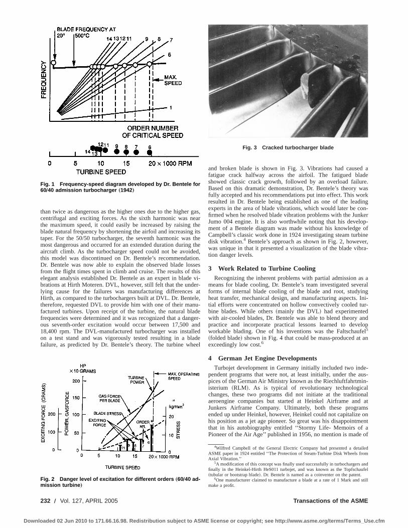
than twice as dangerous as the higher ones due to the higher gas,centrifugal and exciting forces. As the sixth harmonic was nearthe maximum speed, it could easily be increased by raising theblade natural frequency by shortening the airfoil and increasing itstaper. For the 50/50 turbocharger, the seventh harmonic was themost dangerous and occurred for an extended duration during theaircraft climb. As the turbocharger speed could not be avoided,this model was discontinued on Dr. Bentele’s recommendation.Dr. Bentele was now able to explain the observed blade lossesfrom the flight times spent in climb and cruise. The results of thiselegant analysis established Dr. Bentele as an expert in blade vi-brations at Hirth Moteren. DVL, however, still felt that the under-lying cause for the failures was manufacturing differences atHirth, as compared to the turbochargers built at DVL. Dr. Bentele,therefore, requested DVL to provide him with one of their manu-factured turbines. Upon receipt of the turbine, the natural bladefrequencies were determined and it was recognized that a danger-ous seventh-order excitation would occur between 17,500 and18,400 rpm. The DVL-manufactured turbocharger was installedon a test stand and was vigorously tested resulting in a bladefailure, as predicted by Dr. Bentele’s theory. The turbine wheel

and broken blade is shown in Fig. 3. Vibrations had caused afatigue crack halfway across the airfoil. The fatigued bladeshowed classic crack growth, followed by an overload failure.Based on this dramatic demonstration, Dr. Bentele’s theory wasfully accepted and his recommendations put into effect. This workresulted in Dr. Bentele being established as one of the leadingexperts in the area of blade vibrations, which would later be con-firmed when he resolved blade vibration problems with the JunkerJumo 004 engine. It is also worthwhile noting that his develop-ment of a Bentele diagram was made without his knowledge ofCampbell’s classic work done in 1924 investigating steam turbinedisk vibration.4 Bentele’s approach as shown in Fig. 2, however,was unique in that it presented a visualization of the blade vibra-tion danger levels.

3 Work Related to Turbine CoolingRecognizing the inherent problems with partial admission as a

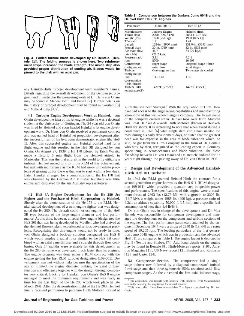
means for blade cooling, Dr. Bentele’s team investigated severalforms of internal blade cooling of the blade and root, studyingheat transfer, mechanical design, and manufacturing aspects. Ini-tial efforts were concentrated on hollow convectively cooled tur-bine blades. While others~mainly the DVL! had experimentedwith air-cooled blades, Dr. Bentele was able to blend theory andpractice and incorporate practical lessons learned to developworkable blading. One of his inventions was the Faltschaufel5

~folded blade! shown in Fig. 4 that could be mass-produced at anexceedingly low cost.6

4 German Jet Engine DevelopmentsTurbojet development in Germany initially included two inde-

pendent programs that were not, at least initially, under the aus-pices of the German Air Ministry known as the Riechluftfahrtmin-isterium ~RLM!. As is typical of revolutionary technologicalchanges, these two programs did not initiate at the traditionalaeroengine companies but started at Heinkel Airframe and atJunkers Airframe Company. Ultimately, both these programsended up under Heinkel, however, Heinkel could not capitalize onhis position as a jet age pioneer. So great was his disappointmentthat in his autobiography entitled ‘‘Stormy Life- Memoirs of aPioneer of the Air Age’’ published in 1956, no mention is made of

4Wilfred Campbell of the General Electric Company had presented a detailedASME paper in 1924 entitled ‘‘The Protection of Steam-Turbine Disk Wheels fromAxial Vibration.’’

5A modification of this concept was finally used successfully in turbochargers andfinally in the Heinkel-Hirth HeS011 turbojet, and was known as the Topfschaufel~tubular or bootstrap blade!. Dr. Bentele is named as a coinventer on the patent.

6One manufacturer claimed to manufacture a blade at a rate of 1 Mark and stillmake a profit.

Fig. 1 Frequency-speed diagram developed by Dr. Bentele for60Õ40 admission turbocharger „1942…

Fig. 2 Danger level of excitation for different orders „60Õ40 ad-mission turbine …

Fig. 3 Cracked turbocharger blade



any Heinkel-Hirth turbojet development team member’s names.Details regarding the overall development of the German jet pro-gram and in particular the pioneering work of Dr. Hans von Ohainmay be found in Meher-Homji and Prisell@2#. Further details onthe history of turbojet development may be found in Constant@3#and Meher-Homji@4,5#.

4.1 Turbojet Engine Development Work at Heinkel. vonOhain developed the idea of his jet engine while he was a doctoralstudent at the University of Go¨ttingen. The 24 year old von Ohainwas hired by Heinkel and soon headed Heinkel’s jet engine devel-opment work. Dr. Hans von Ohain received a permanent contractand was named head of Heinkel jet propulsion development afterthe successful run of his hydrogen demonstrator engine~the HeS1!. After this successful engine run, Heinkel pushed hard for aflight engine and this resulted in the HeS 3B designed by vonOhain. On August 27, 1939, a He 178 piloted by Erich Warsitzmade a historic 6 min flight from the Heinkel airfield inMarienehe. This was the first aircraft in the world to fly utilizing aturbojet. Heinkel rushed to inform the RLM of this achievement,but met with indifference as the RLM had more immediate prob-lems of gearing up for the war that was to start within a few days.Later, Heinkel arranged for a demonstration of the He 178 thatwas observed by the German Air Ministry, but there was littleenthusiasm displayed by the Air Ministry representatives.

4.2 HeS 8A Engine Development for the He 280 JetFighter and the Purchase of Hirth Corporation by Heinkel.Shortly after the demonstration of the He 178 to the RLM, Hei-nkel started development of a twin engine fighter that was desig-nated the He 280. The aircraft could not use engines of the HeS3B type because of the large engine diameter and low perfor-mance. At this time, however, an axial flow engine~designated theHeS 30! that was being developed by Mueller, who had arrived atthe Heinkel Rostock plant, experienced serious development prob-lems. Recognizing that this engine would not be ready in time,von Ohain designed a back-up solution designated the HeS 8which would employ a radial rotor similar to the HeS 3B com-bined with an axial vane diffuser and a straight through flow com-bustor. Only 14 months were available for this development, asthe He 280 airframe was developed much faster than its engines.The engine program was done under a RLM contract with theengine getting the first RLM turbojet designation~109-001!. De-velopment was not without risks because the specification of theaircraft limited the engine diameter making the axial diffuserfunction and efficiency together with the straight through combus-tor very critical. Luckily for Heinkel, von Ohain’s HeS 8 enginemanaged to meet the minimum requirements and was ready intime for the first flight of the He 280 which took place in lateMarch 1941. After the demonstration flight of the He 280, Heinkelfinally received permission to purchase Hirth Motoren located at

Zuffenhausen near Stuttgart.7 With the acquisition of Hirth, Hei-nkel had access to the engineering capabilities and manufacturingknow-how of this well-known engine company. The formal nameof the company created when Heinkel took over Hirth Motorenwas Ernst Heinkel AG-Werk Hirth Motoren~known as Heinkel-Hirth for short!. It is interesting to note that when asked during aconference in 1978@6# what single item von Ohain needed themost during his early development days, he stated that the greatestneed was for expertise in the area of blade vibration which, hesaid, he got from the Hirth Company in the form of Dr. Bentelewho was, by then, recognized as the leading expert in Germanyspecializing in aeromechanics and blade vibration. The closefriendship between Dr. von Ohain and Dr. Bentele endured for 57years right through the passing away of Dr. von Ohain in 1998.

5 Design and Development of the Advanced Heinkel-Hirth HeS 011 Turbojet

In 1942 the RLM granted Heinkel-Hirth the contract for asecond-generation engine known as the HeS 011~RLM designa-tion 109-011!, which provided a quantum step in specific powerand performance. The specifications of this engine were a maxi-mum thrust of 2863 lbs~12.75 kN! with a growth to 3307 lbs~14.7 kN!, a weight under 1985 lbs~900 kg!, a pressure ratio of4.2:1, an altitude capability 50,000 ft~15 km!, and a specific fuelconsumption of less than 1.4 lb/lb-h.

Dr. von Ohain was in charge of the development and Dr. MaxBentele was responsible for component development and man-aged the development on the compressor and turbine sections ofthe engine. The best performance parameters attained by the en-gine in December 1944 were a thrust of 2940 lb~13 kN! at a rotorspeed of 10,205 rpm. The leading particulars of the first genera-tion Jumo 004B engine which was in production and the advancedHeS 011 are compared in Table 1. The engine layout is depicted inFig. 5 ~Neville and Silsbee,@7#!. Additional details on the enginemay be found in Bentele@8#, Hirth-Moteren reports@9,10#, Avia-tion Magazine@11#, US Navy report@12#, Bamford and Robinson@13#, and Carter@14#.

5.1 Compressor Section. The compressor had a singlestage inducer row followed by a diagonal compressor8 ~mixedflow! stage and then three symmetric~50% reaction! axial flowcompressor stages. As the air exited the first axial inducer stage,

7This acquisition was fraught with politics, with Heinkel’s rival Messerschmittreportedly delaying the acquisition for several months.

8This was called ‘‘Kombinationsverdichter,’’ a layout conceived by Dr. vonOhain.

Fig. 4 Folded turbine blade developed by Dr. Bentele. „Ben-tele, †1‡…. The folding process is shown here. Two reinforce-ment strips increased the blade strength. The inside strip alsoprovided proper distribution of cooling air. Blades would bepinned to the disk with an axial pin.

Table 1 Comparison between the Junkers Jumo 004B and theHeinkel Hirth HeS 011 engines

Parameter Jumo 004 B HeS-011A

Manufacturer Junkers Engine Heinkel-HirthThrust ~lbs! 2000 ~8.927 kN! 2863 ~12.75 kN!Weight ~lbs! 1650 ~750 kg! 1950 ~885 kg!T/W ratio 1.21 1.44Length 152-in.~3860 mm! 131.6-in.~3343 mm!Frontal diam 30 in.~760 mm! 32 in. ~805 mm!Air mass flowrate ~lb/s!

46.7~21.2 kg/s!

64 ~29 kg/s!

Pressure ratio 3.1:1 4.2:1rpm 8700 10,205Compressorconfiguration

Eight-stageaxial flow

Diagonal stage1threeaxial stages

Turbineconfiguration

One-stage turbine Two-stage air cooled

Fuelconsumption~lb/lb thrust!

1.4–1.48 1.35

Turbine inlettemperature~F!

1427°F~775°C! 1427°F~775°C!

Journal of Engineering for Gas Turbines and Power APRIL 2005, Vol. 127 Õ 233


the annular passage was reduced by a shaft fairing to the diagonalcompressor. The combination of a diagonal stage with axial flowstages was ingenious as it made the operating line very flat andimparted growth potential without incorporating variable geom-etry that would be required for higher pressure ratios. The double-skinned intake hoods served the dual function of straightening theairflow and housing the accessories, oil tank, and lube oil pump.Both warm air and electric heating were available for anti-icing. Aphotograph of the compressor section showing the mixed flowstage is shown in Fig. 6.

To develop this compressor, a 1600 kW electric test stand inZuffenhausen and a steam turbine driven 15,000 hp stand in Dres-den were utilized. The rigs allowed the measurement of flow,pressure, and temperature distributions in the flow path and con-siderable challenges had to be met in designing the mixed flowcompressor section. Rather than arriving at an optimal configura-tion for the axial stages analytically, this was done experimentallyusing adjustable stators. A variety of settings were tested on thestand and finally this led to satisfactory performance as shown inthe compressor map of Fig. 7~Bentele,@1#!. About half of thetotal pressure ratio of 4.2 was derived by the mixed-flow section~but with moderate efficiency!. The axial stages raised the effi-ciency of the full compressor to 82%. Bentele recounts that duringone test, in spite of smooth running of the engine, the occurrenceof discrepancies in pressure and temperature readings puzzled thetest team. The issue was resolved when a technician appearedholding some broken aluminum blades which he had found at the

compressor air exit and inquired if this might be the problem!Evidently, the uniform breakage of the blades did not result insignificant unbalance.

5.2 Combustor. The combustor was an annular design withairflow being divided into two flow streams by an annular head-piece with a small airflow being routed into the headpiece formixture preparation and combustion. Most of the air was routedthrough two of the outer and inner rows of vanes at the end of thecombustion chamber and into the mixing chamber to attain therequired temperature. The housing wall located around the com-bustor was protected against radiant heat transfer by an annularinsulator around which fresh air from the chamber was circulated.Sixteen equispaced fuel nozzles were utilized with four igniterplugs, two on the lateral axis and two 45° upwards. Bentele indi-cated that the combustor was a great design challenge and obtain-ing a satisfactory radial and circumferential temperature profilewas not easy given the flow profile emanating from the mixedflow compressor wheel. The combustor was, therefore, a workabledesign compromise. Dr. Bentele indicated that the combustor wasone of his most frustrating assignments—he had reservations

Fig. 5 Layout of the HeS 011 engine

Fig. 6 Compressor section of the HeS 011 Fig. 7 HeS 011 compressor map „Bentele, †1‡…



about too much sheet metal being present in the primary andmixing zones and concerns that small sector testing of an annularcombustor would induce false results.9

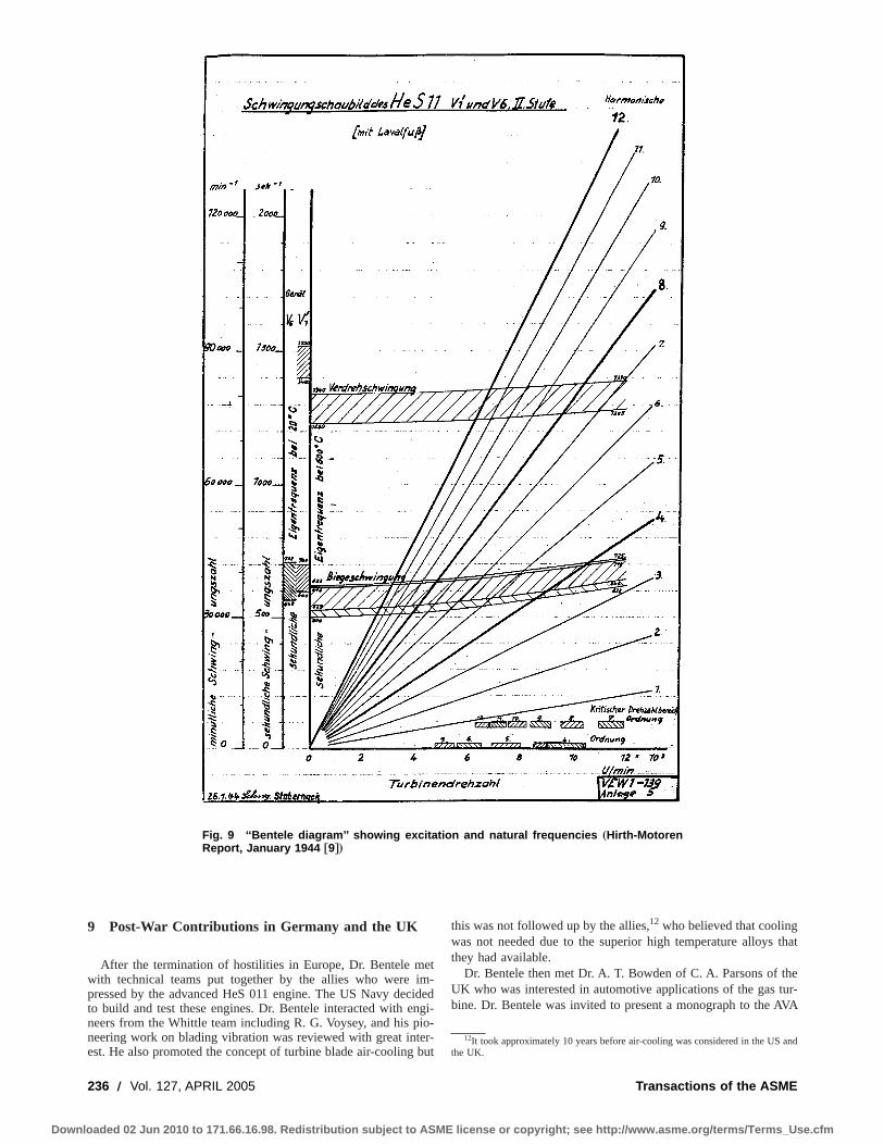
5.3 Turbine Section. The HeS 011 had a remarkable two-stage air-cooled turbine section~Fig. 8! designed by Dr. Max Ben-tele. Two rows of hollow turbine nozzle blades were cooled by airbled off through the annulus after the final compressor stage. Thisnozzle cooling air was ducted between the combustion chamberand the rotor shaft, which was shielded by an annular insert. Bothof the discs had hollow vanes with air being routed to the secondstage through holes bored in the first stage. The airflow exited theblades at the tip. The development of the turbine section was mostchallenging. Initially solid blades were employed and stress rup-ture occurred at the first stage and fatigue failures at the secondstage. The resonance failure was traced to the location of fourstruts of the rear bearing support and these were eliminated byspacing the struts at unequal angles, thus minimizing the forcedexcitations that were in resonance with the second-stage rotorblades. A Bentele Diagram of the blading is depicted in Fig. 9.~Hirth-Motoren report, January 1944@9#!.

The final air-cooled blade designed by Dr. Bentele was called‘‘topfschaufel’’10 and did not utilize any strategic materials. Theseblades were manufactured starting with a circular plate of auste-netic chrome-moly sheet steel from which a closed end tube wasdrawn in several stages with intermediate heat treatments. As seenin Fig. 10~Hirth-Motoren Report, April 1944@10#!, wall thicknessdiminished from 0.079 in.~2 mm! at the root to 0.017 in.~0.45mm! at the blade tip, so as to match the stresses with the prevail-ing radial temperature profile. The airfoil shape was then inducedand finish machining done. Both the first and second turbinestages utilized this construction and contained an insert for theproper distribution of the cooling air and for damping blade vi-bration. Further details of the HeS 011’s construction, accessories,fuels systems, and controls may be found in Meher-Homji andPrisell @2#.

6 Planned Variants and Potential Applications of theHeS 011 Engine

On July 15, 1944, the RLM submitted request for proposalnumber 226/II~known as the ‘‘Emergency Fighter Competition’’!to Germany’s aircraft manufacturers for the second-generation ofjet-powered fighters. The requirements included that this aircraftbe powered by a single Heinkel-Hirth HeS 011 turbojet, operate at

a level speed of 1000 km/h~621 mph! at 7000 m~22,966 ft! andbe armed by four MK 108, 30 mm cannon. The fighter had to havean operating altitude of 14,000 m~45,931 ft!, and have a pressur-ized cockpit. There were several proposals submitted by FockeWulf, Messerschnmitt, Heinkel and Blohm and Voss, with theFocke Wulf Ta-183 being finally selected. The Ta-183 design con-cept is shown in Fig. 11. This design was never built in Germanyas the war ended prior to its development.

7 Resolution of Vibratory Blade Failures on theJunker Jumo 004 B Turbojet

The world’s first production turbojet was the Junkers Jumo 004,which was the powerplant for the Messerschmitt Me-262 fighter~Fig. 12!. The engine was developed by Dr. Anselm Franz and hisdesign team at Junkers. The Jumo was brought from conceptualdesign to production in a span of four years. Details of this enginemay be found in Meher-Homji@5# and Franz@15#. As Franz hadno opportunity to design individual engine components a decisionwas made to design an experimental engine, the 004A, whichwould be thermodynamically and aerodynamically similar to thefinal production engine. The goal in developing the 004A was tohave an operating engine in the shortest time frame without con-sideration for engine weight, manufacturing considerations, orminimizing the use of strategic materials. Based on the results ofthe 004A engine, the production 004B engine was to be built. OnJuly 18, 1942 the first flight of the Me-262 powered by two Jumo004A jets took place and lasted for 12 min.

The Jumo 004B engine was available in June 1943 and duringthe summer, several catastrophic turbine blade failures that re-sulted in aircraft crashes were experienced when operating at fullspeed. The Junkers team worked diligently to resolve the problem.The Air Ministry, getting increasingly concerned with the prob-lem, scheduled a conference at the Junkers Dessau plant in De-cember 1943, to be attended by turbine experts from government,industry, and academia. Max Bentele was asked by the ministry toattend this conference.11 Dr. Bentele listened to the numerous ar-guments pertaining to material defects, grain size, and manufac-turing tolerances. When his turn came, he stated that the underly-ing cause of the problem was excitation induced by the sixcombustor cans and the three struts of the jet nozzle housing afterthe turbine. The combustor and struts excited a sixth-order reso-nance with the blade bending frequency in the upper speed range.The predominance of the sixth-order excitation was due to the sixcombustor cans~undisturbed by the 36 nozzles! and the secondharmonic of the three struts downstream of the rotor. In the 004Aengine, this resonance was above the operating speed range but inthe 004B it had slipped because of the slightly higher turbinespeed and due to the higher turbine temperatures. Dr. Bentele’selegant analysis allowed the problem to be solved by increasingthe blade natural frequency by increasing blade taper, shorteningblades by 1 mm, and reducing the operating speed of the enginefrom 9000 to 8700 rpm. Dr. Bentele’s resolution of this problemhad a major impact on the operational availability of the Me-262.

8 Blade Design Recommendations on the BMW 003Turbojet

BMW also produced an axial flow turbojet engine~BMW 003!with a thrust of 2,000 lbs~907 kg!. The engine had a seven-stageaxial compressor with a pressure ratio of 3:1, an annular combus-tor, and an air cooled turbine that had a very unusual disk attach-ment as shown in Fig. 13. This attachment was plagued by failuresand Dr. Bentele was consulted to resolve the problem. Dr. Bentelefound the design overly complex, with the wedge and pin beingunnecessary because the centrifugal forces would have held theblade in place. He made several suggestions that allowed trouble-free operation.

9When engine runs confirmed this opinion, the combustor was given severalnicknames—‘‘Guinea pig,’’ ‘‘rat’s tail’’ and worse! The time was not ripe for anannular combustor of short length, low pressure drop, and high efficiency.

10This was a scaled derivitave of the ‘‘topfschaufel’’ invented by Dr. Bentele forturbocharger turbines. 11At 34 years of age, Dr. Bentele was the youngest person to speak up.

Fig. 8 Photo of the HeS 011 two-stage air-cooled turbinesection



9 Post-War Contributions in Germany and the UK

After the termination of hostilities in Europe, Dr. Bentele metwith technical teams put together by the allies who were im-pressed by the advanced HeS 011 engine. The US Navy decidedto build and test these engines. Dr. Bentele interacted with engi-neers from the Whittle team including R. G. Voysey, and his pio-neering work on blading vibration was reviewed with great inter-est. He also promoted the concept of turbine blade air-cooling but

this was not followed up by the allies,12 who believed that coolingwas not needed due to the superior high temperature alloys thatthey had available.

Dr. Bentele then met Dr. A. T. Bowden of C. A. Parsons of theUK who was interested in automotive applications of the gas tur-bine. Dr. Bentele was invited to present a monograph to the AVA

12It took approximately 10 years before air-cooling was considered in the US andthe UK.

Fig. 9 ‘‘Bentele diagram’’ showing excitation and natural frequencies „Hirth-MotorenReport, January 1944 †9‡…



on the feasibility of the gas turbine as a vehicle power plant. Thismonograph covered several investigations of compressor configu-rations, regenerators, and other practical aspects and included atreatment of regeneration, water injection, ceramic materials, andthe concept of a vehicular gas turbine. Because of his contribu-tions to this and other studies, Dr. Bentele was offered a contractfrom the British Ministry of Supply~MoS! to work on a gasturbine tank engine project that was being developed at Parsons.He contributed significantly to the mechanical design of the en-gine and in resolving several problems. Dr. Bentele’s contribu-tions included the design of a mechanical control system and ther-mal shock investigations. Because of the special transientoperating regime of a tank engine, Dr. Bentele started a systematic

Fig. 10 Ingenious method of developing air-cooled turbine blade starting with a cir-cular plate 25 mm diameter „Hirth Motoren GmbH report, April 1944 †10‡…

Fig. 11 Focke Wulf TA-183 with HeS 011 engine



investigation into the thermal shock aspects of turbine blading.The study included an analysis of thermal stresses in a slab forstatic conditions of constant heat flow and constant temperaturedifference. Four different materials were considered. Thereafter,transient conditions were modeled where the surface temperatureswere suddenly changed. The resulting calculations and modelswere then extended to shapes approaching those of turbine bladesto arrive at a qualitative relationship for the number of thermalcycles to failure. Dr. Bentele and his group verified his thermalshock investigations in test rigs with actual turbine nozzles oftheir tank engine. The test rigs developed allowed testing to ex-amine the cyclic thermal behavior of blading and combustorwalls. A detailed paper was published by Dr. Bentle and Mr.Lowthian @16# which appeared in the February 1952 issue of‘‘Aircraft Engineer.’’ This paper drew an important analogy be-tween thermal shock and vibration phenomena in showing thatsurface condition, heat treatment, ageing, and varying the ampli-tude of the applied load had similar effects.

10 Work at Heinkel-Hirth „1952–1956…After his stay in the UK, Max Bentele was persuaded by Ernest

Heinkel to rejoin Heinkel at the Stuttgart plant, as Chief of De-velopment. He joined Heinkel in 1952 and Ernst Heinkel relied onhis expertise in managing a variety of technical and business is-sues. Dr. Bentele worked on a range of development initiatives onreciprocating engines and motor scooters that Heinkel was mak-ing. Heinkel’s heart was, however, set on aviation and he tried tobuild a team to work on engines. On Heinkel’s request, Dr. Ben-tele served as a consultant to a project involving a gas turbineutilizing thermal compression.13 Heinkel’s most ambitious project

was the design of a jet fighter and its engine. The engine wasdesignated as the HeS 053 and borrowed features from theHeS011, and SNECMA’s Atar engines. Ultimately the engine andfighter projects were cancelled. In 1955 Curtiss Wright offered Dr.Bentele a job and Dr Bentele emigrated to the USA in 1956 wherehe joined the Wright Aeronautical Division~WAD! of Curtiss-Wright.

11 Contributions at Curtiss-WrightAt Curtiss-Wright Dr. Bentele worked on several projects in-

cluding detailed studies on turbine blade cooling and transpirationcooling. Several experimental results were developed on a test rigenabling Curtiss-Wright to replace the two-stage turbine designfor the J65 engine with a single stage air-cooled design. Thisdevelopment was, however, too late to be put into production. Dr.Bentele was appointed Manager of Mechanical Components foradvanced gas turbines and made contributions to blade vibrationscaused by forced excitation, rotating stall, and aeroelastic flutter.

In May of 1958, on a Friday afternoon, Dr. Bentele was calledinto the office of Roy T. Hurley~the President and Chairman ofCurtiss-Wright!. Hurley handed him a crude plastic 536.5 in.model of an engine and said ‘‘That’s supposed to be an engine.Find out over the weekend whether it is, and its pros and cons.Report to me on Monday and don’t talk to anybody about it!’’ OnMonday, Dr. Bentele reported his findings in detail to Hurley andthen learned that its inventor was Felix Wankel. This was the startof Dr. Bentele’s important involvement with this rotary engine andCurtiss-Wright’s position as it exclusive licensor of NorthAmerica. Max Bentele is recognized as an important figure in thedevelopment of the Wankel engine and made major contributionsto its design. In 1966 he was granted a patent on this engine forburning of a wide range of fuels. By 1966, Curtiss-Wright stoppedengine manufacture and restructured itself to be to a major sup-plier of components to the aerospace and other industries.

12 Contributions at Avco LycomingIn May of 1967, Dr. Bentele joined Avco Lycoming as Consult-

ing Engineer to the Vice President of Engineering. During hiscareer and prior to his retirement in 1974 he made several impor-tant contributions including the following.

1. Solutions to major service problems with the T53 and T55engines.14 Dr. Bentele spearheaded investigation of a rash ofdisk failures where tennons of aluminum disks holding bladedovetail roots were breaking causing engine failure. In rec-ognition of his worldwide reputation and integrity, Dr. Ben-tele was selected by the Army Aviation Systems Command~AVSCOM! to chair a blue ribbon panel to find a solution tothe problem. It was determined that a failure mode includedstress-rupture, high cycle fatigue caused by blade vibrations,and low cycle fatigue due to frequent takeoffs and landing ofthe helicopter. The solution was a replacement of the diskswith a one-piece welded rotor made of titanium.

2. Development studies of low-power gas turbine engines. Dr.Bentele worked on a 5 lbs/s flow class gas turbine configu-ration with a single spool compressor consisting of one axialand one centrifugal stage driven by a single stage axial tur-bine, a reverse-flow annular combustor, and a power turbine.Details of Dr. Bentele’s investigations may be found in Ben-tele and Laborde@17#.

3. Testing of turbine containment failures. In the fall of 1970 acontainment failure occurred on a T55 engine where powerturbine blades had broken off and the bearing support failedunder the massive unbalance situation, resulting in controlsystem damage. Dr. Bentele devised an iterative testing

13This concept was originally conceived by Dr. Hans von Ohain and had beeninvestigated theoretically and experimentally at Heinkel. The post-war project wasrun by Max Adolf Muller.

14These helicopter engines were the branchildren of Dr. Anselm Franz, designerof the Junker Jumo 004 turbojet that powered the world’s first production fighter, theMe-262.

Fig. 12 The Me-262 powered by two Junker Jumo 004B turbo-jets. Dr. Bentele was instrumental in resolving a major opera-tional blade vibration problem with this engine.

Fig. 13 Complex blade root design for the BMW 003 enginethat resulted in fatigue cracks and failures



method by which stress-rupture failures could be induced atan exact speed thus reducing the number of very expensivetests to a minimum.

13 ClosureThe long and distinguished career of Dr. Max Bentele has been

covered, with an emphasis on his pioneering work on turbojetengines. During WW II he worked on the development of theadvanced HeS 011 engine. He made seminal contributions in thearea of blade vibration, blade fabrication, air cooling, and turbojetdesign. While not focused on in this paper, his significant contri-butions to the development of the Wankel engine earned him thetitle of the father of the Wankel engine in the USA. A photographof Dr. von Ohain, Sir Frank Whittle, and Dr. Max Bentele isshown in Fig. 14. This photograph taken in 1987, is the lastknown photograph of these jet pioneers together. Dr. Bentele isFellow of the SAE, Associate Fellow of AIAA and member of theVDI. He holds 12 patents. In 1971 The University of Wyominginvited Dr. Bentele to place his technical material in their Ameri-can Heritage Center. This was done in 1972, thus preserving valu-able documents and reports of his contributions to gas turbine andaviation engine technology. Dr. Bentele has been awarded manyhonors over the years culminating in 2001, with the prestigiousASME R. Tom Sawyer Award, the citation of which reads: ‘‘Forpioneering work in the development of aeroengines and technicalcontributions in the areas of turbine blade fatigue analysis, bladecooling, and control systems for gas turbine rotary regenerators.’’

For his seminal work on jet engines that started at the dawn ofthe turbojet revolution, Dr. Bentele will always be remembered asa pioneer of the jet age.

AcknowledgmentsWe wish to thank Dr. Max Bentele, for his communications and

his correspondence over the years in which he answered severalquestions and queries about his early work on turbojets. His ex-cellent autobiography ‘‘Engine Revolutions’’ has been a valuablereference and covers several fascinating details of the dawn of thejet age in which he played a pivotal role.

References@1# Bentele, M., 1991,Engine Revolutions: The Autobiography of Max Bentele,

SAE, Warrendale, PA.@2# Meher-Homji, C. B., and Prisell, E., 1999, ‘‘Pioneering Turbojet Develop-

ments of Dr. Hans von Ohain—From the HeS1 to the HeS 011,’’ ASME GasTurbine and Aeroengine Conference, Indianapolis, ASME Paper No: 99-GT-228; also in J. Eng. Gas Turbines and Power122~2!, p. 191 April 2000.

@3# Constant, E. W. II, 1980,The Origins of the Turbojet Revolution, John Hop-kins University Press, Baltimore, MD, 1980.

@4# Meher-Homji, C. B., 2000, ‘‘The Historical Evolution of Turbomachinery,’’Proceedings of the 29th Turbomachinery Symposium, Texas A&M University,Houston, TX, September 2000.

@5# Meher-Homji, C. B., 1996, ‘‘The Development of the Junkers Jumo 004B—the World’s First Production Turbojet,’’ 1996 ASME Gas Turbine andAeroengine Conference, Birmingham, UK, June 10–13, 1996. ASME PaperNo. 96-GT-457. Also in ASME Transactions of Gas Turbines and Power1194,October 1997.

@6# ‘‘An Encounter Between the Jet Engine Inventors Sir Frank Whittle and Dr.Hans von Ohain,’’ 1978, Wright-Patterson Air Force Base, OH, History Office,Aeronautical Systems Division, US Air Force Systems Command.

@7# Neville, L. E., and Silsbee, N. F., 1948,Jet Propulsion Progress, McGraw-Hill, New York, 1948.

@8# Bentele, M., 1989, ‘‘Das Heinkel-Hirth Turbostrahltriebwerk HeS011—Vorganger, Characteristiche Merkmale Erkenntnisse,’’ Proceedings of Confer-ence on 50 Years of Jet-Powered Flight, Sponsored by the DGLR~GermanSociety for Aeronautics and Astronautics!, DGLR Publ. No. 89-05, October26–27, 1989, Deutsches Museum, Munich, Germany.

@9# Hirth-Motoren GmbH Report, April 1944, VEW 1-139, ‘‘Schwingungsunter-suchungen an der HeS 11—Turbine V1 aund V6 mit Vollschaufeln,’’ dated Jan31, 1944; Max Bentele Papers, American Heritage Center, University of Wyo-ming.

@10# Hirth-Motoren GmbH Report, April 1944B, VEW 1-140, ‘‘Untersuchung derFussbefestigung von Topf und Falt-Schaufeln durch Kaltschleuderprufung,’’dated April 16, 1944; Max Bentele Papers, American Heritage Center, Univer-sity of Wyoming.

@11# ‘‘Design of the German 109-011 A-O Turbojet,’’ Aviation, September, 1946.@12# ‘‘Basic Technical Data on the 109-011 Jet Engine A-O Development Series,’’

U.S. Navy Department Bureau of Aeronautics, Third Edition, December 1944.@13# Bamford, L. P., and Robinson, S. T., 1945, ‘‘Turbine Engine Activity at Ernst

Heinkel Atiengesellschaft Werk Hirth-Motoren, Stuttgart/Zuffenhausen,’’ Re-port by the Combined Intelligence Objectives Sub-committee dated May 1945.

@14# Carter, J. L., 1945,Ernst Heinkel Jet Engines, Aeronautical Engine Laboratory@AEL#, Naval Air Experimental Station, Bureau of Aeronautics, US Navy, June1945.

@15# Franz, A., 1979,The Development of the Jumo 004 Turbojet Engine, 40 Yearsof Jet Engine Progress, edited by Boyne, W. J. and Lopez, D. S., National Airand Space Museum, Smithsonian, Washington, 1979.

@16# Bentele, M., and Lowthian, C. S., 1952, ‘‘Thermal Shock Tests on Gas TurbineMaterials,’’ Aircraft Engineering, February, 1952, pp. 32–38.

@17# Bentele, M., and Laborde, J., 1972,Evolution of Small Turboshaft Engines,National SAE Aerospace Engineering and Manufacturing Conference, San Di-ego, CA, October 2–5, 1972, SAE Paper No. 720830.

Fig. 14 Photograph of three jet engine pioneers taken in 1987.Left to right Sir Frank Whittle, Dr. Hans von Ohain, and Dr. MaxBentele.



Robert P. CzachorChief Consulting Engineer, Structures,

GE Aircraft Engines,One Neumann Way,

Cincinnati, Ohio 45215e-mail: [email protected]

Unique Challenges for BoltedJoint Design in High-BypassTurbofan EnginesBolted joints are used at numerous locations in the rotors and carcass structure of modernaircraft turbine engines. This application makes the design criteria and process substan-tially different from that used for other types of machinery. Specifically, in addition toproviding engine alignment and high-pressure gas sealing, aircraft engine structuraljoints can operate at high temperatures and may be required to survive very large appliedloads which can result from structural failures within the engine, such as the loss of a fanblade. As engine bypass ratios have increased in order to improve specific fuel consump-tion, these so-called ‘‘Ultimate’’ loads increasingly dominate the design of bolted joints inaircraft engines. This paper deals with the sizing and design of both bolts and leverflanges to meet these demanding requirements. Novel empirical methods, derived fromboth component test results and correlated analysis have been developed to performstrength evaluation of both flanges and bolts. Discussion of analytical techniques in useincludes application of the LS-DYNA™ code for modeling of high-speed blade impactevents as related to bolted joint behavior.@DOI: 10.1115/1.1806453#

Introduction

This paper deals with a number of unique challenges that largecommercial turbofan engines present for the design of boltedjoints which secure the engine carcass and rotor components.These circumferential casing/rotor joints typically utilize flat-faced lever-type flanges. Figure 1 illustrates the locations ofbolted joints in a typical turbofan engine.

The basic behavior of bolted joints@1# in turbofan engines un-der normal operation are common to other applications and willnot be discussed here. Unique to the turbofan engine, however, areconstraints on diameter due to weight and packaging concerns,along with challenging internal pressures, rotational speeds andtemperature levels. Transient operation during engine starts, accel-eration or deceleration, along with aircraft maneuvers subjectthese joints to numerous combinations of loads in the course ofnormal engine operation. In addition, the designs must accommo-date so-called ‘‘ultimate’’ loading conditions, such as the largeimbalance forces generated by abusive rotor imbalance. Such im-balance can result from loss of a fan blade due to bird strike orother cause. In that event, damage to the joints is acceptable butcarcass integrity of the engine generally must be maintained tosatisfy FAA requirements. With the latest generation engine fandiameters growing as large as 129 in.~328 cm!, these ultimateloads have increased to a point where bolted joints in commercialturbofan engines must push the state of the art to a much moresignificant extent than in common industrial applications.

Industrial practice@2# provides a basis for sizing bolted jointsbased primarily on providing adequate sealing against internal liq-uid or gas pressure. These methods are conservative enough that,in many cases, externally applied loads may safely be ignored. Incontrast, the design of aircraft engine bolted joints is dominatedby the external loads the joint must support. While leakage controlis still a requirement, adequate sealing usually results as the jointis designed to meet other requirements—rarely is it a governing

factor in the sizing of the joint. Experience has shown that avariety of design requirements must be satisfied by the aircraftengine joint, including:

1. Prevent joint separation under applied loads during normaloperation;

2. Provide transverse-load capability to prevent slippage bymeans of sufficient joint clamp and flange friction;

3. Prevent air/fluid leakage;4. Provide strength sufficient to support limit/ultimate dynamic

loads due to abusive rotor unbalance;5. Low cycle fatigue~LCF! life in excess of expected engine

lifetime;6. High-cycle fatigue~HCF! life sufficient to preclude failure

with expected levels of normal engine vibration;7. Provide strength sufficient to support loads due to limit/

ultimate aircraft maneuvers.

Preload and Residual PreloadAssembly of joints for turbofan engines is usually performed

with the common torque wrench. Variables such as friction coef-ficients, assembler technique and torque wrench calibration per-mits control of clamp only within630%. When more accuracy isnecessary, torque-angle techniques have been used to reduce thisvariation to620%, but this requires specialized tooling for fas-tener assembly. Assembly lubricants, such as synthetic engine oilor graphite grease, have been shown to be effective in minimizingclamp variation.

The available clamp is determined through component testingin order to determine the torque-tension or angle-tension relation-ship. These tests are performed either with force washers or withultrasonic measurements of bolt elongation. The latter techniquerequires tensile calibration of the ultrasonic extensometers foreach particular type of fastener. Ultrasonic measurement has theadvantage of permitting the determination of fastener clamp onproduction engine assemblies, rather than in the laboratory, whichthen includes the variables of technician lubrication and assemblytechnique.~In rare cases, ultrasonic measurement of bolt exten-sion during production assembly has been used to insure clampvariation of less than65%.!

During engine operation, three effects serve to reduce this ini-tial assembly clamp. The first is simply thermal expansion, since

Contributed by the International Gas Turbine Institute~IGTI! of THE AMERICANSOCIETY OF MECHANICAL ENGINEERSfor publication in the ASME JOURNAL OFENGINEERING FOR GAS TURBINES AND POWER. Paper presented at the Interna-tional Gas Turbine and Aeroengine Congress and Exhibition, Atlanta, GA, June16–19, 2003, Paper No. 2003-GT-38042. Manuscript received by IGTI, October2002, final revision, March 2003. Associate Editor: H. R. Simmons.

240 Õ Vol. 127, APRIL 2005 Copyright © 2005 by ASME Transactions of the ASME


the fasteners, flanges and any attached bracketry will generally notbe made from the same material or operate at the same tempera-ture for engine steady-state or transient conditions. This clamploss can be simply expressed as:

DB52KETH aBDTBlb2aNDTNhn2(l

NF

~aFDTFt f ! iJ (1)

Note that the joint combined stiffness term,KET has been used toaccount for the load division between bolt load and joint clamp. Aless accurate expression, often found in the literature, simply usesthe bolt stiffness,KET

B .A second issue leading to preload loss in turbomachinery is the

contraction of the flange thickness due to transverse normalstresses. Tensile hoop stress will exist in a circumferential casingflange due to internal pressure or in a rotating flange due to speed.Flange radial stress levels can also be significant due to thermalgradients. Both will cause Poisson’s contraction of the flangethickness and create a further loss in clamp, which can be ex-pressed as:

DB52KET(l

NF

$m~sR1sH!~ t fn/EET

F,n!%n (2)

Equations~1! and ~2! are derived in Appendix A.A less obvious effect comes about from the change in the elastic

modulus of the joint materials with temperature. A bolted joint issimply a mechanical arrangement of springs and when the jointmaterials are brought to elevated temperature levels, the change inspring constants due to the reduction in material modulus willcreate a further loss in preload. This change in bolt load can beexpressed as:

DB5BRT$KET /KRT21% (3)

Interestingly, while this effect does reduce the clamp at operatingconditions, it alone may not result in a change in bolt strain.Because of this, the cyclic content of bolt stress which is due tothe modulus change at temperature in many cases can be safelyignored in the calculation of fastener low-cycle fatigue capability.A derivation of Eq.~3! and an explanation of the effect on boltstrain is provided in Appendix B.

Many characteristics of turbomachinery bolted joint behavior,at least for normal operation, are dependent on the availableclamp at operating conditions. Given the variation in assemblyclamp and the factors operating to reduce it, providing adequateclamp during engine operation is often a challenge.

Applied Loads in OperationBolted joints in turbomachinery are subjected to a variety of

loads in operation that can be broadly categorized as:

1. Axisymmetric loads due to internal pressure, thermal gradi-ents, torque and rotational speed. These loads can act bothnormal and transverse to the bolt axis.

2. Asymmetric loads or beam-bending loads on the engine,which can be created by rotating imbalance forces, aircraftmaneuvers~Including gyroscopic effects from the rotatingturbomachinery!, aerodynamic forces acting on the engineinlet and nacelle, and the engine thrust.~Since the enginethrust is produced at the engine centerline and reacted at theengine mounts which are offset from the centerline, enginecarcass bending results.!

3. Impact loads resulting from failure events where blade frag-ments may impact the casings in the vicinity of flanges.

Loading conditions are further categorized according to the like-lihood of the event and different design criteria applied accord-ingly. For example, we might require that the joint not separate~lose clamp at the bolt centerline! for normal engine transient andsteady state operation combined with normal aircraft maneuverswhereas for a major failure event the criteria would be simply thatthe flanges and fasteners not fracture.

It can be seen then, that the designer will be faced with theconstruction of a number of combined load cases for a given jointthat must be evaluated against the appropriate design criteria forthat condition. These load cases will involve the combination ofaxisymmetric loads with beam moments and shears due to bothmaneuvers and imbalance, which will often act in different planes.This often precludes determination of the most limiting bolt loca-tion in a joint by simple inspection. It is then necessary to calcu-late the load on each individual fastener in the joint in order toidentify the most highly-loaded fastener.

Furthermore, the load combination/condition and relevant de-sign criteria that will in the end size a given joint will not beknown at the point the design is initiated. All possible loadingsmust be evaluated against the appropriate design criteria before itis established whether a design is satisfactory or otherwise.

Design Criteria for Normal OperationExperience has shown that the following criteria must be satis-

fied for a durable bolted joint when normal operation of the en-gine and aircraft are considered:

1. Maintain an axial flexibility ratio (RaET) of less than 0.5, i.e.,

maintain the clamping member stiffness at no more than50% of the clamped members. This minimizes cyclic loadson the bolt and improves fatigue life.

2. Provide sufficient bolt length, even where thin flanges arejoined, by use of a spacer~thick washer! in the joint. Thisboth improves the joint axial flexibility ratio and ensuressufficient stretch of the bolt at assembly to desensitize thejoint from small embedment losses. Longer bolts, having agreater total strain to failure than short bolts, also afford thejoint greater ultimate load capability, as will be discussedlater in this paper.

3. Provide sufficient clamp to prevent separation of the joint atoperating conditions. This criterion ensures adequate seal-ing, predictable structural stiffness, and satisfactory boltlow-cycle fatigue life.

Fig. 1 Structural bolted joints in a typical turbofan engine



4. Provide sufficient clamp/flange face friction coefficients topreclude transverse movement of the flanges. Even verysmall amounts of transverse displacement of the flanges inthe clamped condition will produce very high bolt bendingstresses and inevitable failure.

5. Related to these criteria is the philosophy that observation ofany evidence of movement, such as wear or entrapped de-bris, at a joint following engine cyclic endurance testing is aclear indication of an unsatisfactory joint design. It has beenfound that, due to the cyclic nature of aircraft engine opera-tion, even small amounts of movement at a joint will inevi-tably produce wear, which leads to loss of clamp, increasedmovement and additional wear until failure results.

Ultimate Load Capability: Empirical MethodsHaving satisfactorily sized a joint to meet the requirements of

normal operation, the designer must then examine the ultimateload capability of the joint. Little conservatism is possible consis-tent with engine weight and space constraints. The design crite-rion is quite simple: The loadpath must remain intact. First, wecan examine the problem of a bolt under ultimate loading condi-tions which usually results from a large overturning moment~OTM! engine beam-bending load. Such loads can result from anextreme aircraft maneuver or rotor imbalance condition.

A conventional, elastic calculation would simply determine themaximum local shell load associated with the most highly-loadedbolt due to the applied bending load using the formula:

PSHELL52M

NRS(4)

The derivation of Eq.~4! is provided in Appendix C.Accounting for the lever action created by the fact that the bolt

is offset from the line of action of the shell@3#

BAPPLIED5PSHELLF11l

bG (5)

Typically, the joint would be past the point of separation on thejoint diagram~Fig. 3! for this ultimate condition so preload is notconsidered in the calculation. The formulation assumes two-dimensional behavior of the circumferential flange and has beenfound to be reasonably accurate for flanges 20 in.~51 cm! indiameter or larger. The toe reaction at the outer edge of the flangeis then simply:

R5BAPPLIED2PSHELL (6)

A conservative calculation would then simply compare the result-ing bolt stress to the bolt material ultimate strength. Note thesesimple calculations ignore bolt bending, since, by definition, thebolt is strained near its elongation limit in tension so that littlebending capability remains.

Component testing has shown that such elastic calculations arequite conservative. The initial explanation was that a shift in theneutral axis of bending would bring more bolts to their ultimatecapability, thus increasing the overall strength of the joint. Asillustrated in Fig. 2, this neutral axis shift results since the jointcompression load path, which is simply through the heel of theflange where the shells abut, is considerably stiffer than the tensileload path through the bolt, where flange lever action and boltelongation contribute to substantially more flexibility. Since thejoint stiffness in the compressive direction is greater than that intension, a shift in the neutral axis of bending results in loadingadditional bolts in tension as shown. An additional contributor isbolt plasticity, since the most highly loaded bolt will not fail whenloaded to its ultimate capability, but must also undergo a strainequal to its tensile elongation capability prior to fracture. Theseeffects are illustrated in Fig. 2, where elastic/perfectly plastic be-havior has been assumed for the bolts.

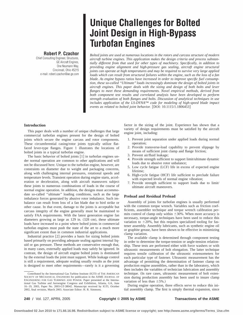
However, experimental measurements of neutral axis shift dur-ing component tests failed to reveal the magnitude of shift neces-sary to account for the observed joint capability. An additionaleffect, observed from elastic-plastic joint analysis, was that theflange lever action, as described by Eq.~5!, decreased when sig-nificant bolt plastic strain occurred. The joint diagram for the mosthighly loaded bolt was found to be described by Fig. 3, which isextended significantly beyond that loading considered in conven-tional calculations.

Figure 3 describes the load history of the most highly loadedbolt in a joint as the OTM load is applied. Initially, the assemblyclamp is reduced as the thermal effects discussed in the previoussection occur~point A!. As engine normal operating load is ap-plied, the load is absorbed primarily by joint compression reliefand some additional bolt load in conventional fashion as describedin Ref. @1# ~point B!. Note that the bolt load in normal operation isactually less than at cold assembly since the thermal effects dis-cussed earlier dominate, rather than the applied load. For normaloperation of the turbomachinery, this behavior is typical for hightemperature joints. However, what interests us more is the behav-ior beyond this point.

As the load is further increased, the slope of the bolt load ver-sus applied load changes at the point of separation~point C!where all clamp at the bolt centerline is relieved. However, theflange toe is still in contact due to the flange lever action and thetoe reaction is present. As load is increased further and the boltplastically deforms, the compressive force at the flange toe isrelieved, in much the same way as the clamp at the bolt centerlineis relieved during the early stages of loading, reducing the slope ofthe loading curve~point D!. In this fashion, flange lever action isdecreased. By reducing the rate of bolt load increase with appliedload at the most highly loaded bolt, the strength of the joint isenhanced as the load is redistributed to the adjacent, less highly-loaded bolts in much the same manner as occurs due to the neutralaxis shift. Both these effects thus combine to afford a much higherjoint ultimate load capability than the simple elastic calculationwould suggest.

The point of bolt failure~point E! is determined by the totalamount of plastic strain that the most highly loaded bolt can sus-tain. Thus, an explanation for the increased strength of joints withlonger bolts is provided. The larger the bolt total elongation capa-bility, the more redistribution of load that will occur and thegreater the ultimate strength of the joint.

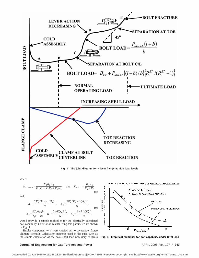
Data from a number of component tests and correlated elastic-plastic analysis was interrogated, with the aim of providing asimple means for bolt sizing for ultimate load conditions. It wasassumed that the basic behavior would be governed by the ratio ofthe joint tensile stiffness to the compression stiffness. The testdata was examined and it was found that a quadratic fit using theflange parameter:

KFLANGE /KSHELL (7)

Fig. 2 Neutral axis shift mechanism for overturning momentloading



where

KFLANGE5K1K2K3

K1K21K2K31K1K3and KSHELL5

K4K5

K41K5(8)

and,

K152EET

F,1RBp~ t f1/ l 1!3

N, K25

2EETF,2RBp~ t f

2/ l 2!3

N,

(9)

K35EET

B ATHb

l B~ l 1b!K45

2pRs1ts

1EETF,1

NK55

2pRs2ts

2EETF,2

N

would provide a simple multiplier for the elastically calculatedbolt capability. Correlation results using this parameter are shownin Fig. 4.

Similar component tests were carried out to investigate flangeultimate strength. Calculation methods used in the past, such asthe simple calculation of the peak shell load necessary to stressFig. 4 Empirical multiplier for bolt capability under OTM load

Fig. 3 The joint diagram for a lever flange at high load levels



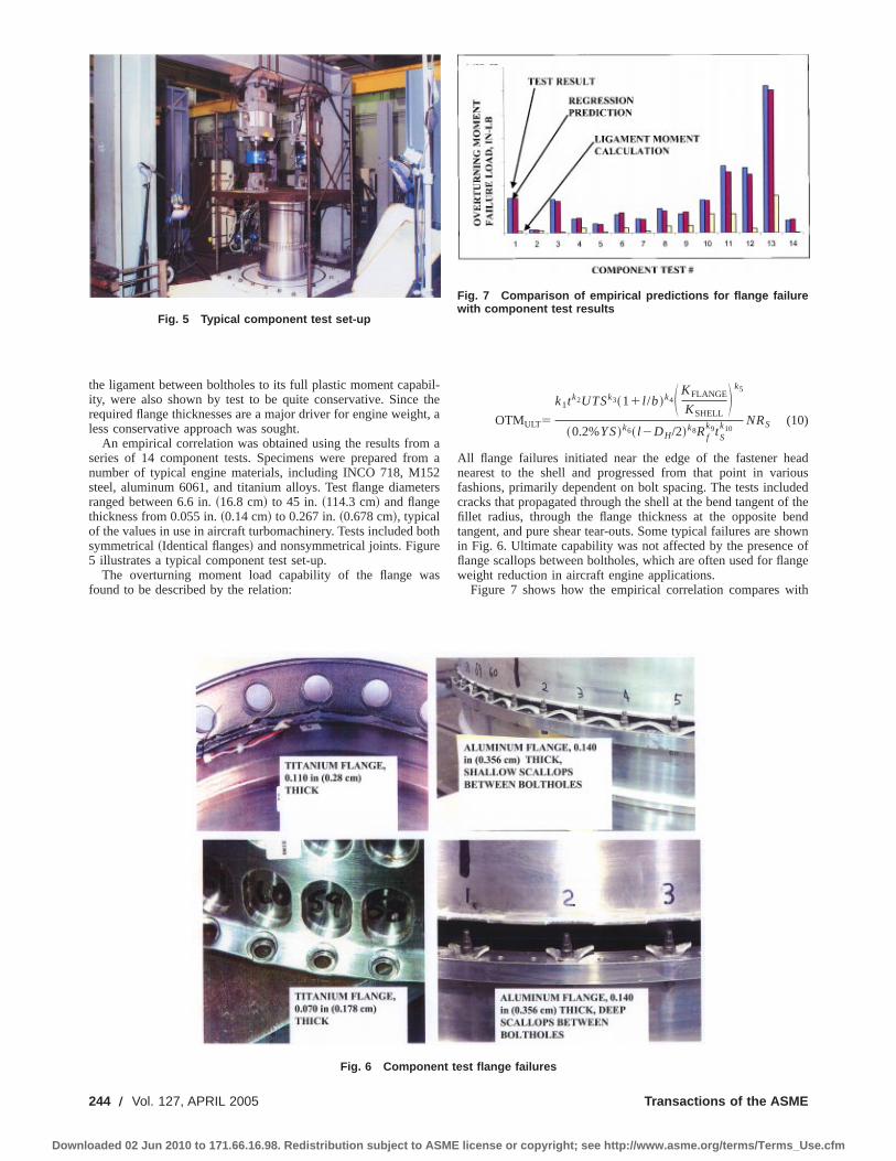
the ligament between boltholes to its full plastic moment capabil-ity, were also shown by test to be quite conservative. Since therequired flange thicknesses are a major driver for engine weight, aless conservative approach was sought.

An empirical correlation was obtained using the results from aseries of 14 component tests. Specimens were prepared from anumber of typical engine materials, including INCO 718, M152steel, aluminum 6061, and titanium alloys. Test flange diametersranged between 6.6 in.~16.8 cm! to 45 in. ~114.3 cm! and flangethickness from 0.055 in.~0.14 cm! to 0.267 in.~0.678 cm!, typicalof the values in use in aircraft turbomachinery. Tests included bothsymmetrical~Identical flanges! and nonsymmetrical joints. Figure5 illustrates a typical component test set-up.

The overturning moment load capability of the flange wasfound to be described by the relation:

OTMULT5

k1tk2UTSk3~11 l /b!k4S KFLANGE

KSHELLD k5

~0.2%YS!k6~ l 2DH/2!k8Rfk9tS

k10NRS (10)

All flange failures initiated near the edge of the fastener headnearest to the shell and progressed from that point in variousfashions, primarily dependent on bolt spacing. The tests includedcracks that propagated through the shell at the bend tangent of thefillet radius, through the flange thickness at the opposite bendtangent, and pure shear tear-outs. Some typical failures are shownin Fig. 6. Ultimate capability was not affected by the presence offlange scallops between boltholes, which are often used for flangeweight reduction in aircraft engine applications.

Figure 7 shows how the empirical correlation compares with

Fig. 5 Typical component test set-up

Fig. 6 Component test flange failures

Fig. 7 Comparison of empirical predictions for flange failurewith component test results



the actual component test results. Also shown for comparison is aconventional handbook fully-plastic moment capability calcula-tion.

Analytical Methods for Ultimate CapabilityAs it may be imagined, a degree of conservatism must be in-

cluded in any empirical component-test based approach to jointdesign, which is undesirable from a weight standpoint and willnecessarily underpredict actual joint capability. Component testssuch as described in this paper are both expensive and time-consuming and therefore are not a desirable option as a designtool, particularly in light of efforts to shorten time-to-market ofturbomachinery products. Therefore, an effort was undertaken todevelop Finite-Element analysis techniques to predict flange andbolt ultimate load capability. An important part of this effort wasto show correlation between the analysis and component test re-sults.

The ANSYS® program was used. The general features of thefinite element model shown to correlate well for purposes of boltcapability calculation are illustrated in Fig. 8. This is a relativelysimple 3D plate model of a 180° sector of the flanged connection.Gap elements are used at the flange faces and elastic-plastic linkelements represent the bolts. The bolt is modeled including an

additional length to represent the bolt head and nut flexibility.Otherwise, the model is linear. Details such as bolt holes andflange fillet radii are not modeled. Sufficient shell length is in-cluded to attenuate the effect of boundary conditions.

The model is loaded incrementally and failure is predictedwhen the bolt link elements reach the plastic failure strain level asestablished by fastener component tests. This strain value is com-puted from a standard tensile strength test based on the assump-tion that the measured bolt strain is uniform over the clampedlength of the fastener including the dummy length included toaccount for the head and nut flexibility effects. In reality, theplastic strain in a fastener is concentrated in the first few threadspast the nut washer face, but, since the fastener is not modeled indetail, the use of the average plastic extension over this completelength has been used. While a seemingly crude representation ofthe problem, such models have shown excellent correlation to testresults for bolt failure prediction.

Analytical prediction of flange ultimate capability has provenmuch more difficult. Simple models such as shown in Fig. 8,when used to predict flange failure, were found to deviate fromcomponent test results by as much as a factor of 2. It was estab-lished that very detailed models were required to simulate thecomplex interaction between the flanges and the fastener. Detailmodeling of the bolt head or nut in contact with the flanges wasrequired along with the inclusion of friction in the solution suchthat relative movement of the joint elements could occur. An ex-ample of the type of model necessary to accurately predict flangeultimate failure is shown in Fig. 9. All elements of this modelhave plastic properties. Such analysis starts to challenge even cur-rent computational capability. Models constructed to this level of

Fig. 8 Simple plate-beam model used for prediction of boltOTM capability

Fig. 9 Complex model required for accurate prediction offlange capability

Fig. 10 LS-DYNA® analysis of a bolted joint in the vicinity of a blade impact on the adjacent casing



detail have achieved correlation with component test resultswithin 15% of the actual failure load. In some cases, correlationwithin less than 2% has been achieved.

This same, more complex model can, of course, also be used tocalculate the ultimate capability of the bolts, although simplermodels per Fig. 8 suffice for that purpose.

The Impact Problem for Blade ContainmentA final unique category of bolted joint loads in turbomachinery

is that which occurs following a blade failure when the releasedblade strikes the engine casing with great force. While the casingsare designed to prevent blade penetration, bolted joints in thevicinity of the impact will see high loads due to casing deforma-tion during the initial portion of the event, followed by theimbalance-induced cyclic bending loads discussed earlier in thispaper. Plastic, radial deflection of the fan casing of over 2 in.~5cm! will occur in the case of metallic fan casings used on largecommercial engines. In order to ensure that the blade or bladefragments are contained and engine carcass integrity is main-tained, gross failure of the joints must be prevented during theblade impact although some loss of individual fasteners is accept-able.

The LS-DYNA™ code has been used successfully to predictjoint capability under these impact conditions. A model of theengine casing and rotor is run to simulate the blade release, fol-lowed by a submodel analysis of a local group of the most highly-loaded fasteners. Shown in Fig. 10 is the sequence of events pre-dicted for an engine/inlet joint for a large fan engine following therelease of a fan airfoil and its containment by the casing immedi-ately adjacent to the flange.

The entire sequence of events shown in Fig. 10 occurs in lessthan 8 ms. Since all elements in the model behave in an elastic-plastic fashion with known failure elongation, failure of any jointelement can be directly predicted. Use of high strain-rate materialdata is necessary for an accurate analysis due to the short durationof the event.

ConclusionsBolted joints in turbomachinery are designed to maintain clamp

and sealing capacity under normal engine operating conditions,much like other industrial applications. They also must remainintact under extremely high loads associated with engine failureevents. Significant insight has been gathered regarding the behav-ior of lever-flange bolted joints for these severe loading conditionsthat aid the designer in achieving the necessary capability withinthe space and weight constraints of the aircraft engine application.~See Fig. 11.!

AcknowledgmentsThe author would like to gratefully acknowledge the efforts of

E. Baehre, S. Bhattacharjee, A. Mishra, J. Renners, S. Ross, and F.Worthoff as well as the earlier work of C. K. Coombs, all ofwhom made significant contributions to the work describedherein.

Nomenclature

aN 5 nut thermal coefficient of expansionaB 5 bolt thermal coefficient of expansionaF 5 flange thermal coefficient of expansionDB 5 change in bolt load from assembly condition

D l RT-ETB 5 change in bolt length from assembly condition to

elevated temperature conditionDTB 5 delta bolt temperature from assembly conditionDTf 5 delta flange temperature from assembly conditionDTN 5 delta nut temperature from assembly condition

sH 5 hoop, or circumferential flange stresssR 5 Radial flange stressm 5 Flange Poisson’s ratio

0.2%YS 5 0.2% yield strengthATH 5 thread equivalent area

b 5 distance from bolt centerline to flange free edge,also known as toe distance

BAPPLIED 5 bolt load due to applied external loads in the sepa-rated condition, i.e., without preload

BET 5 residual preload at operating conditions consideringtemperature effects

BRT 5 assembly bolt loadEET

B 5 Young’s modulus of bolt at elevated temperatureEET

F,n 5 Young’s modulus of flange n at elevated tempera-ture

DM 5 thread minor diameterhn 5 nut heightkn 5 empirical constant

KRT 5 joint combined spring constant at elevated tempera-ture KRT5KB

RT/(11RaRT)

KET 5 joint combined spring constant at room temperatureKET5KB

ET/(11RaET)

KFLANGE 5 spring value representing flange flexibility in theflange parameter used for bolt OTM capability

KSHELL 5 spring value representing shell flexibility in theflange parameter used for bolt OTM capability

KETSP 5 stiffness of a spacer or washer

KRTB 5 series spring combination of the bolt, nut, and

spacer stiffness at room temperatureKET

B 5 series spring combination of the bolt, nut, andspacer stiffness at elevated temperature

KETF 5 series spring combination of the flange stiffness at

elevated temperatureKRT

F 5 series spring combination of the flange stiffness atroom temperature

Kn 5 spring parameter in the flange parameter used forbolt OTM capability

Fig. 11 Lever flange joint geometry

Fig. 12 Representation of thermal and Poissions mechanismfor a bolted joint



KETS 5 stiffness of the shell portion of the flange at el-

evated temperaturel b 5 bolt effective length; This usually the clamped

~grip! length increased by a distance 0.8DM to ac-count for the flexibility of the bolt head and thethreads extending into the nut

l 5 lever distance from casing shell centerline to boltcenterline

RaET 5 the axial flexibility ratio for the joint at elevated

temperature,KETB /KET

F

RaRT 5 the axial flexibility ratio for the joint at room tem-

perature,KRTB /KRT

F

M 5 applied overturning moment load or engine beam-bending moment

N 5 number of fasteners in the jointNF 5 number of flanges in the joint

OTMULT 5 the overturning moment at the point of flange orbolt failure

PSHELL 5 maximum shell load at a single bolt due to an ap-plied over-turning moment

R 5 toe reaction forceRB 5 radius to bolt circleRf 5 fillet radius size between the shell and flange faceRS

n 5 radius to shell centerline associated with flangenS 5 distance of neutral axis shiftt fn 5 flange thickness of flangen

tSn 5 shell thickness associated with flangen

Appendix A: the Effect of Thermal Expansion andFlange Poisson’s Contraction on Bolt Loadat Temperature

Both these phenomena, as described by Eqs.~1! and~2!, can berepresented schematically by considering the bolt deflection~d!resulting from a change in flange thickness (D l ) as shown in Fig.12.

For the bolt, it can be seen that:

BET5BRT2dKETB (11)

DB52dKETB (12)

For the flange,

DB5$D l 2d%KETF (13)

Therefore,

d5KET

F D l

KETB 1KET

(14)

Substituting into~12!

DB52KET

F KETB

KETB 1KET

D l (15)

Using the definition of the joint combined spring constant,

KET5KB

ET

~11RaET!

(16)

We obtain:

DB52KETD l (17)

For thermal expansion, we can consider the change in flangethickness relative to the bolt,

D l 5H aBDTBlb2(l

NF

~aFDTFt f ! i2aNDTNhnJ (18)

Substitution of Eq.~18! into Eq. ~17! yields Eq.~1!.

Considering the effects of Poisson’s contraction of the flanges,we obtain the change in flange thickness as:

D l 5(l

NF

$m~sR1sH!~ t fn/EET

F,n!%n (19)

Substitution of Eq.~19! into Eq. ~17! yields Eq.~2!.

Appendix B: the Effect of Elevated Temperature Modu-lus on Bolt Load and Strain

To determine the impact of the change in modulus on a boltedjoint as it is brought to an elevated temperature, we can considerbolt and flange materials with either an identical, or zero, coeffi-cient of expansion but with temperature-dependent moduli. If weconsider the fact that any change in bolt length from the as-sembled condition to the elevated temperature condition musthave an equal change in the clamped length of the flange we canwrite the equation:

BRT

KRTB

2BET

KETB

5BET

KETF

2BRT

KRTF

(20)

Rearranging this equation yields an expression for the bolt load attemperature:

BET5BRTKET

F KETB ~KRT

F 1KRTB !

KRTF KRT

B ~KETF 1KET

B !(21)

The left-hand side of Eq.~20! represents the change in bolt lengthat temperature due solely to the change in modulus. If we substi-tute Eq.~21! into ~20!, we obtain:

D l RT2ETB 5

BRT

KRTF

2BRTKET

F ~KRTF 1KRT

B !

KRTF KRT

B ~KETF 1KET

B !(22)

Reducing further,

D l RT2ETB 5

BRT

KRTF H 12

KETF ~KRT

F 1KRTB !

KRTF ~KET

F 1KETB !

J (23)

This quantity becomes zero if:

H KETF

KRTF J H KRT

B

KETB J 51 (24)

For a given geometry, the stiffness terms in Eq.~24! are onlydependent on the modulus. Therefore, if the bolt and flange areconstructed of the same materials, or from materials with similarmodulus response to temperature, little or no change in bolt strainresults from the change in modulus of the joint materials.

Returning to Eq.~21!, we can write:

BET5BRT

KETB $11KRT

B /KRTF %

KRTB $11KET

B /KETF %

(25)

Rearranging further, we obtain

BET5BRT

@KETB /$11KET

B /KETF %#

@KRTB /$11KRT

B /KRTF %#

(26)

Using the definition of the axial flexibility ratio,

Ra5KRTB /KRT

F (27)

we obtain

BET5BRT

$KETB /11Ra

ET%

$KRTB /11Ra

RT%(28)

Using the definition of the combined joint spring constant,



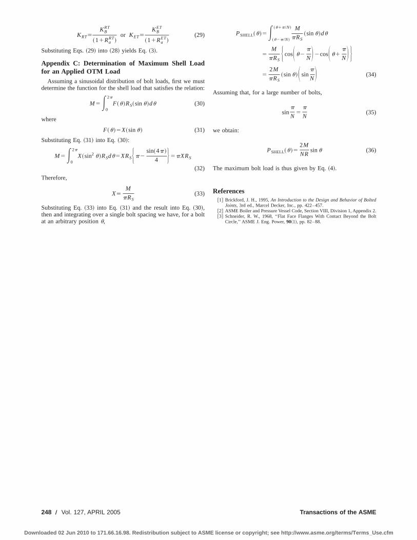
KRT5KB

RT

~11RaRT!

or KET5KB

ET

~11RaET!

(29)

Substituting Eqs.~29! into ~28! yields Eq.~3!.

Appendix C: Determination of Maximum Shell Loadfor an Applied OTM Load

Assuming a sinusoidal distribution of bolt loads, first we mustdetermine the function for the shell load that satisfies the relation:

M5E0

2p

F~u!RS~sinu!du (30)

where

F~u!5X~sinu! (31)

Substituting Eq.~31! into Eq. ~30!:

M5E0

2p

X~sin2 u!RSdu5XRSH p2sin~4p!

4 J 5pXRS

(32)

Therefore,

X5M

pRS(33)

Substituting Eq.~33! into Eq. ~31! and the result into Eq.~30!,then and integrating over a single bolt spacing we have, for a boltat an arbitrary positionu,

PSHELL~u!5E~u2p/N!

~u1p/N! M

pRS~sinu!du

5M

pRSH cosS u2

p

ND2cosS u1p

ND J5

2M

pRS~sinu!S sin

p

ND (34)

Assuming that, for a large number of bolts,

sinp

N5

p

N(35)

we obtain:

PSHELL~u!52M

NRsinu (36)

The maximum bolt load is thus given by Eq.~4!.

References@1# Brickford, J. H., 1995,An Introduction to the Design and Behavior of Bolted

Joints, 3rd ed., Marcel Decker, Inc., pp. 422–457.@2# ASME Boiler and Pressure Vessel Code, Section VIII, Division 1, Appendix 2.@3# Schneider, R. W., 1968, ‘‘Flat Face Flanges With Contact Beyond the Bolt

Circle,’’ ASME J. Eng. Power,90~1!, pp. 82–88.



Abd. Rahim Abu Talib1

e-mail: [email protected] Putra Malaysia,

Department of Aerospace Engineering,Faculty of Engineering,

43400 Selangor, Malaysia

Andrew J. Neely1

University of New South Wales,School of Aerospace and Mechanical

Engineering,Australian Defense Force Academy,

Northcott Drive,Canberra ACT 2600, Australia

e-mail: [email protected]

Peter T. IrelandUniversity of Oxford,

Department of Engineering Science,Parks Road,

Oxford OX1 3PJ, UKe-mail: [email protected]

Andrew J. MullenderRolls-Royce plc.,

Fire Precautions Group,P.O. Box 31,

Derby, DE24 8Bj, UKe-mail: [email protected]

Detailed Investigation of HeatFlux Measurements Made in aStandard Propane-AirFire-Certification BurnerCompared to Levels Derived Froma Low-Temperature AnalogBurnerThis paper presents detailed heat flux measurements on a flat plate subjected to theISO2685 [The International Organization for Standardization (ISO), 1992, ‘‘Aircraft—Environmental Conditions and Test Procedures for Airborne Equipment—Resistance toFire in Designated Fire Zones,’’ ISO2685:1992(E)] standard, propane fueled burner usedthroughout the industry in aero-engine fire-certification. The authors have developed acustom-built heat transfer gauge to measure the heat flux from the burner under isother-mal wall conditions. The heat flux from the standard burner is normally calibrated usingeither a water-cooled copper tube or a Gardon gauge, each sited at a single position inthe flame. There are no reports in the literature of a detailed survey of heat flux distribu-tion for the burner and the results are of considerable interest to engineers involved infire-certification. The reported measurements constitute the first, detailed distribution ofheat flux from the actual burner flame during a fire test. These measurements providedbenchmark data which allowed the heat flux distribution from the ISO burner to becompared to levels derived from the low-temperature analog burner developed by theauthors. The analog burner uses liquid crystals to measure heat transfer coefficient andadiabatic wall temperature on scale models of engine components and provides key datato facilitate the successful design of components used in fire zones. The objective of thispaper is to further validate the low-temperature analog burner technique developed by theauthors which simulates the standard large propane-air burner for fire-certification inaero engine. @DOI: 10.1115/1.1806454#

1 Introduction

1.1 ISO2685 Propane-Air Burner. The ISO propane-airburner is widely used in the UK to certify critical engine compo-nents exposed to the danger of fire in aircraft engines. The alter-native, Kerosene burner, which is frequently used in the US, isalso specified in ISO2685@1# and in FAA report@2#. In the stan-dard structural fire-test, engine components are immersed in theflame from the ISO burner for a period of 15 min to establish ifthey are fireproof. This is to verify the structural integrity of thecomponents under flame attack. Therefore it is essential to studythe detailed distribution of heat flux within the burner flame.While a full three-dimensional survey would provide the mostdetail, as the standard specifies a test plane for the location ofcomponent surfaces 75 mm downstream from the burner face, thetwo-dimensional distribution of heat flux at this location is ofprimary interest.

The large propane-air burner consists of a plenum chamber,

burner head and burner face. Mixed propane-air is supplied by373 copper tubes to the burner head and cooling air is dischargedvia 332 smaller holes interspersed with the copper tubes in theburner face~Fig. 1!. The faceplate acts as a flame stabilizer toprevent back flow into the burner head. The flow rate of the gasand air are adjusted to produce the standard flame characteristic.The ISO standard requires the flame to have the following char-acteristics: temperature: 1100°C680°C; heat flux density: 116kW m22610 kW m22.

ISO2685@1# requires that the burner flame temperature must bewithin the required tolerance over at least 25% of the burner area.To this end a rake of thermocouples of specified type and size isrecommended. This rake measurement is normally only per-formed at the single horizontal line specified. During such a cali-bration, it can be observed that the thermocouples radiate signifi-cantly ~Fig. 2!. Neely et al. @3# reports that due to the largediameter of the thermocouple recommended for the calibration,the effect of radiation from the thermocouple tip significantly re-duces the temperature measured in the flame. Once the measuredtemperature readings~;1100°C! have been corrected for the ra-diation losses, the actual peak flame temperature is found to beapproximately 1900°C, as would be expected from an equilibriumflame calculation. It is noted by the authors that this significantdifference between the actual flame temperature and that specifiedin the standard is not widely understood within the industry.

ISO2685 @1# also requires that the heat flux in the standard

1Formerly at the Department of Engineering Science, University of Oxford, ParksRoad, Oxford OX1 3PJ, UK.




burner must be calibrated using either a water-cooled copper tubecalorimeter or an alternative approved calorimeter. The specifiedcalibration method can only measure a steady heat flux and alsohas a very slow response. It requires a 3 min warm-up timebeforethe temperature measurements taken. The temperature history ofthe constant flow of water is monitored for a period of 3 minand used to calculate the average heat flux using the followingequation:

Q5urcpDT

A(1)

whereQ is the amount of heat supplied from the flame,u is thevolume flow rate of the water,r is the water density,cp is thespecific heat of water,DT is the temperature difference, andA isthe area of the cylinder. This calibration method only provides asingle measurement of heat flux integrated over the length of theimpingement of the flame onto the copper tube.

1.2 Heat Flux Measurement. There are many methods ofmeasuring heat flux such as those reported in Schultz and Jones@4#, Jones@5#, and Ainsworth et al.@6#. However these methodsare unsuitable for surveying the ISO2685@1# standard flame. Agauge for this purpose must be able to accurately measure the heatflux up to approximately 200 kW m22 and be able to withstandprolonged immersion in a 1900°C flame. For this reason, thin filmgauges~TFGs! were chosen to measure the surface temperature ofan enamelled-insulating layer attached to a water-cooled metallicplate. As well as maintaining the gauges at a manageable surface

temperature, the cooled enclosure accurately prescribes the ther-mal boundary condition by removing the large step in surfacetemperature between the gauge and its surroundings seen for un-cooled surrounds such as ceramic sheeting.

Thin film gauges were selected to measure the surface tempera-ture due to their fast response and negligible influence on thesurface flow field. Additionally they are able to endure elevatedsurface temperatures.

1.3 Low-Temperature Analog Technique. In order to re-duce the reliance on conventional fire testing, a new technique hasbeen developed at the University of Oxford, which is faster,cheaper, and provides test data at higher resolution than the stan-dard fire test~Mullender et al.@7#!. Initial testing of engine com-ponent models using the low temperature technique demonstratedgood agreement with metal temperatures from actual ISO burnertests. The validation and development of the low-temperature ana-logue burner technique is discussed in details by Neely et al.@3,8,9# and Abu Talib et al.@10#.

In this approach the high temperature standard fire test~nomi-nally 1900°C! is replaced by tests at close to ambient temperature~approximately 80°C! in which accurate plastic models, surfacecoated with thermochromic liquid crystal, are immersed in theflow from the low-temperature analog burner to enable the map-ping of heat transfer coefficient,h, and adiabatic wall temperature,Taw, across the surface of the model. The heat transfer coefficientdistributions are then input as boundary conditions into a finite-element thermal analysis code, together with knowledge of thecomponent heat-loss due to radiation and where applicable cool-ing from the by-pass flow, to permit full thermal modeling of thebehavior of the component during fire attack.

2 Test Facilities and InstrumentationThis section provides detailed descriptions of the instrumenta-

tion used in the heat flux measurements and the experimentalconfiguration.

2.1 Thin Film Gauge. Thin film gauges are widely used tomeasure transient and steady state heat transfer. Since the 1970sthe technique has been developed and used in a variety of gasturbine applications such as those described in Jones@11,12#. Fur-ther application and development of the traditional TFG are de-scribed by Epstein@13#, Doorly and Oldfield@14,15#, and Dunn@16#.

A TFG can be used to measure surface temperature and localheat flux when it is used in conjunction with an insulating sub-strate. The heat transfer rate can be obtained from the steady stateone-dimensional conduction equation as follows:

q5DTS k

DxD (2)

wherek is the substrate thermal conductivity,Dx is the thicknessof the substrate andDT is the temperature difference across thesubstrate. The temperatureDT across a sheet of known thermalproperties and dimensions is measured with the traditional sput-tered gauge sensor and a thermocouple is located on the bottomside of this insulating layer in a metal test model. The thermo-couple is placed as close as possible to the metal surface. Thedevelopment of the direct heat transfer gauge is fully explained byPiccini et al.@17#.

The TFGs used in the current work consisted of platinum films~approximately 0.04mm thick! painted onto the surface of anenamelled Inconel disc~50 mm diameter and 2 mm thick! ~Fig.3!. Each platinum TFG is approximately 5 mm long and 1 mmwide. The enamel is assumed to have properties similar to fusedquartz with thermal conductivity of approximately 1.36W m21 K21 ~Doorly @18#!. Inconel-600~nickel/chromium alloy!,which has a good oxidation resistance at high temperature and hasa thermal conductivity of 14.8 W m21 K21 at room temperature,

Fig. 1 ISO2685 standard large „propane-air … fire-test burner †1‡

Fig. 2 ISO burner temperature calibrations



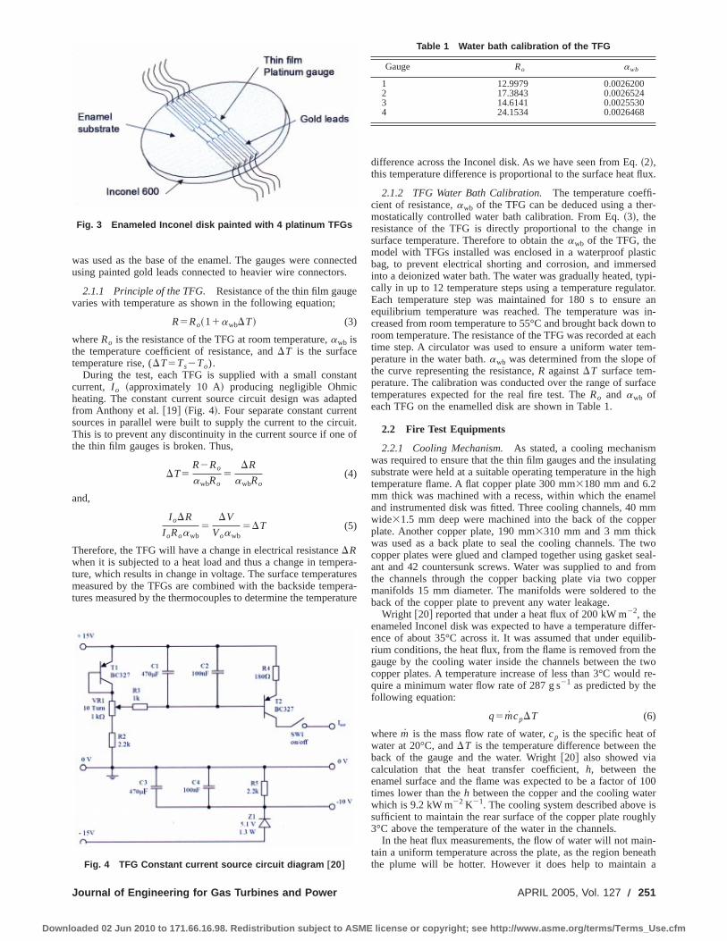
was used as the base of the enamel. The gauges were connectedusing painted gold leads connected to heavier wire connectors.

2.1.1 Principle of the TFG. Resistance of the thin film gaugevaries with temperature as shown in the following equation;

R5Ro~11awbDT! (3)

whereRo is the resistance of the TFG at room temperature,awb isthe temperature coefficient of resistance, andDT is the surfacetemperature rise, (DT5Ts2To).

During the test, each TFG is supplied with a small constantcurrent, I o ~approximately 10 A! producing negligible Ohmicheating. The constant current source circuit design was adaptedfrom Anthony et al.@19# ~Fig. 4!. Four separate constant currentsources in parallel were built to supply the current to the circuit.This is to prevent any discontinuity in the current source if one ofthe thin film gauges is broken. Thus,

DT5R2Ro

awbRo5

DR

awbRo(4)

and,

I oDR

I oRoawb5

DV

Voawb5DT (5)

Therefore, the TFG will have a change in electrical resistanceDRwhen it is subjected to a heat load and thus a change in tempera-ture, which results in change in voltage. The surface temperaturesmeasured by the TFGs are combined with the backside tempera-tures measured by the thermocouples to determine the temperature

difference across the Inconel disk. As we have seen from Eq.~2!,this temperature difference is proportional to the surface heat flux.

2.1.2 TFG Water Bath Calibration.The temperature coeffi-cient of resistance,awb of the TFG can be deduced using a ther-mostatically controlled water bath calibration. From Eq.~3!, theresistance of the TFG is directly proportional to the change insurface temperature. Therefore to obtain theawb of the TFG, themodel with TFGs installed was enclosed in a waterproof plasticbag, to prevent electrical shorting and corrosion, and immersedinto a deionized water bath. The water was gradually heated, typi-cally in up to 12 temperature steps using a temperature regulator.Each temperature step was maintained for 180 s to ensure anequilibrium temperature was reached. The temperature was in-creased from room temperature to 55°C and brought back down toroom temperature. The resistance of the TFG was recorded at eachtime step. A circulator was used to ensure a uniform water tem-perature in the water bath.awb was determined from the slope ofthe curve representing the resistance,R againstDT surface tem-perature. The calibration was conducted over the range of surfacetemperatures expected for the real fire test. TheRo and awb ofeach TFG on the enamelled disk are shown in Table 1.

2.2 Fire Test Equipments

2.2.1 Cooling Mechanism.As stated, a cooling mechanismwas required to ensure that the thin film gauges and the insulatingsubstrate were held at a suitable operating temperature in the hightemperature flame. A flat copper plate 300 mm3180 mm and 6.2mm thick was machined with a recess, within which the enameland instrumented disk was fitted. Three cooling channels, 40 mmwide31.5 mm deep were machined into the back of the copperplate. Another copper plate, 190 mm3310 mm and 3 mm thickwas used as a back plate to seal the cooling channels. The twocopper plates were glued and clamped together using gasket seal-ant and 42 countersunk screws. Water was supplied to and fromthe channels through the copper backing plate via two coppermanifolds 15 mm diameter. The manifolds were soldered to theback of the copper plate to prevent any water leakage.

Wright @20# reported that under a heat flux of 200 kW m22, theenameled Inconel disk was expected to have a temperature differ-ence of about 35°C across it. It was assumed that under equilib-rium conditions, the heat flux, from the flame is removed from thegauge by the cooling water inside the channels between the twocopper plates. A temperature increase of less than 3°C would re-quire a minimum water flow rate of 287 g s21 as predicted by thefollowing equation:

q5mcpDT (6)

wherem is the mass flow rate of water,cp is the specific heat ofwater at 20°C, andDT is the temperature difference between theback of the gauge and the water. Wright@20# also showed viacalculation that the heat transfer coefficient,h, between theenamel surface and the flame was expected to be a factor of 100times lower than theh between the copper and the cooling waterwhich is 9.2 kW m22 K21. The cooling system described above issufficient to maintain the rear surface of the copper plate roughly3°C above the temperature of the water in the channels.

In the heat flux measurements, the flow of water will not main-tain a uniform temperature across the plate, as the region beneaththe plume will be hotter. However it does help to maintain a

Fig. 3 Enameled Inconel disk painted with 4 platinum TFGs

Fig. 4 TFG Constant current source circuit diagram †20‡

Table 1 Water bath calibration of the TFG

Gauge Ro awb

1 12.9979 0.00262002 17.3843 0.00265243 14.6141 0.00255304 24.1534 0.0026468



steady temperature for the duration of the measurements, as theequilibrium temperature will be reached more quickly. Further-more it also allows high representative heat fluxes to be measuredat low manageable surface temperatures as in the actual tests.

2.2.2 Traversing Mechanism.The hollow water-cooled cop-per plate was flush mounted within a 600 mm3600 mm33 mmthick steel fire shield. This was done to both protect the vulnerablepiping, instrumentation wiring and traversing mechanism fromflame impingement and to provide a uniform flat-plate boundarycondition across the full extent of the survey. The thin steel fireshield was strengthened by vertical and horizontal ribs to preventit from buckling. The copper plate was mounted onto a translatingframe, which allowed vertical and horizontal traverses. The framewas built in such way to provide a smooth movement for the heatflux measurements to be taken across the flame~Fig. 5!.

3 Heat Flux Measurements ProcedureThis section provides detailed descriptions of the heat flux cali-

bration and the fire test measurements procedure.

3.1 Heat Flux Calibration. The termk/Dx from Eq. ~2!must be experimentally calibrated due to the uncertainty in theenamel thickness, thermal properties and the unknown heat trans-fer properties of the interface between the Inconel and the buriedthermocouples. The TFG heat flux gauge was calibrated at lowtemperature against two calibrated micro-foil heat flux~Micro-foilheat flux sensor—RdF Corporation, 23 Elm Ave, P.O Box 490,Hudson, NH 03051-0490! sensors as shown in Fig. 6.

The sensors were flush mounted on the enamel surface adjacentto the TFG. A low level of heat flux was applied by a hot air gunand assumed to penetrate the micro-foil heat flux gauge and plati-num film equally. Traversing the gauges through the plume coreand using only the observed peak values compensated for nonuni-formities in the heat flux distribution from the hot air plume. It isnoted that micro-foil heat flux sensors were prone to damage atthe higher surface temperatures and were therefore not suitable foruse in the actual flame experiments. During the calibration, a con-stant flow of water was supplied into the copper plate to maintaina steady manageable surface temperature at the TFGs for the highlevels of heat flux representative of the ISO burner flame. Thevoltage signals from the TFGs were amplified to enable a betteraccuracy of the calibration since the voltage changes were verysmall ~approximately 0.5mV!.

The surface temperature of the enamel was calculated using theknowledge ofRo and awb . The temperature difference betweenthe surface temperature and the temperature measured by the ther-mocouple underneath the enamel were used in conjunction withthe heat flux measured from the thermopile sensors to determinean equivalent thermal conductivity to thickness ratiok/Dx of thesubstrate.

3.2 Fire Test Procedure. The experimental measurementswere conducted at a private commercial fire testing cell in the UK.The ISO propane-air burner was set up so as not to impinge on thetest plate and ignited. The burner setting was adjusted to get thecorrect fuel and air mass flow rates and flame temperatures speci-fied by the standard. At the same time, the water to the copper testplate was turned on and was left for approximately 5 min to allowthe plate to reach an equilibrium temperature. The data logger wasset to continuously record the voltage signals from the TFGs andalso the temperature signals from the thermocouples underneaththe enameled disk.

To begin the test, the ISO burner was rotated so that the flameimpinged directly onto the TFGs on the test plate as shown in Fig.5. The distance between the burner face and the surface of theTFG was set at 75 mm to conform with ISO2685@1#. The instru-mented plate was moved horizontally and vertically to 29 loca-tions across one half of the test plane, which covered an area ofapproximately 0.036 m2. It was assumed that the burner flame wasnominally symmetrical about a vertical axis. Each location washeld for 60 s while the TFG voltage level was recorded. An initialtransient voltage was observed as the cooled gauges reached anew equilibrium temperature. The voltage signals were later aver-aged over the observed equilibrium period for each 60 s step.During the experiment, condensation occurred in front of thecooled copper plate generating a thin film of water dripping to thefloor. It is noted that this exothermic condensation process wouldbe expected to have artificially increased the surface temperaturereadings. It is also noted that this condensation process would alsoinitially occur on any component being heated from ambient tem-perature in a standard fire test.

4 Heat Flux DistributionThe heat flux from the ISO burner can now calculated using

information obtained from the heat flux calibration,k/Dx and thehistory of the change in temperature,DT during the fire test. Thecombination of the value ofk/Dx, obtained from the heat fluxcalibration, with the distribution of temperature differences acrossthe heat flux sensor, measured in the flame, enables the calculationof the distribution of heat flux to an ambient surface in the ISOburner flame. Figure 7 shows the distribution of heat flux at thetest plane across one half of the ISO burner plume. It can be seenthat the heat flux distribution from the ISO burner was found to belower than the specified values required by the standard and themost likely reason for this is given later. Knowledge of distribu-tion of heat flux in the burner plume can be used to benchmark themeasurements of local convective heat transfer coefficient madein the test plane of the low-temperature analog burner.

In order to compare the heat flux levels derived from both thelow-temperature test and the actual fire-test, the surface tempera-

Fig. 5 Side view schematic of fire test set upFig. 6 TFG water-cooled heat flux gauge system



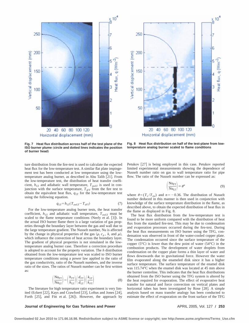
ture distribution from the fire-test is used to calculate the expectedheat flux for the low-temperature test. A similar flat plate impinge-ment test has been conducted at low temperature using the low-temperature analog burner, as described in Abu Talib@21#. Fromthe low-temperature test, the distribution of heat transfer coeffi-cient, hLT and adiabatic wall temperature,TawLT is used in con-junction with the surface temperature,TsFT from the fire test toobtain the equivalent heat flux,qLT for the low-temperature testusing the following equation.

qLT5hLT~TawLT2TsFT! (7)

For the low-temperature analog burner tests, the heat transfercoefficient, hLT and adiabatic wall temperature,TawLT must bescaled to the flame temperature conditions~Neely et al.@3#!. Inthe actual ISO burner flame there is a large variation of gas prop-erties through the boundary layer between the gas and wall due tothe large temperature gradient. The Nusselt number, Nu is affectedby the change in physical properties of the gas~r, cp , k, andm!,which influence the convection of heat across the boundary layer.The gradient of physical properties is not simulated in the low-temperature analog burner case. Therefore a correction procedureis adopted to account for the property variation. Theh distributionobtained from the low-temperature test was scaled to ISO burnertemperature conditions using a power law applied to the ratio ofthe gas conductivity, ratio of the Nusselt numbers, and the inverseratio of the sizes. The ratios of Nusselt number can be first writtenas:

S NuFT

NuLTD5S hFT

hLTD S dFT

dLTD S kLT

kFTD (8)

The literature for high temperature ratio experiment is very lim-ited ~Eckert@22#, Kays and Crawford@23#, Loftus and Jones@24#,Forth @25#, and Fitt et al. @26#!. However, the approach by

Petukov @27# is being employed in this case. Petukov reportedlimited experimental measurements showing the dependence ofNusselt number ratio on gas to wall temperature ratio for pipeflow. The ratio of the Nusselt number can be expressed as:

S NuFT

NuLTD5un (9)

where u5(Ts /Taw) and n520.36. The distribution of Nusseltnumber deduced in this manner is then used in conjunction withknowledge of the surface temperature distribution in the flame, asdescribed above, to obtain the expected distribution of heat flux inthe flame as displayed in Fig. 8.

The heat flux distribution from the low-temperature test isfound to be more uniform compared with the distribution of heatflux from the standard fire-test. This may be due to condensationand evaporation processes occurred during the fire-test. Duringthe heat flux measurements on ISO burner using the TFG, con-densation was observed in front of the water-cooled copper plate.The condensation occurred since the surface temperature of thecopper~5°C! is lower than the dew point of water~54°C! in thecombustion products. The development of water droplets fromcondensation on the copper plate forms a thin layer of water andflows downwards due to gravitational force. However the waterfilm evaporated along the enameled disk since it has a highersurface temperature. The surface temperature of the enamel diskwas 115.74°C when the enamel disk was located at 45 mm abovethe burner centreline. This indicates that the heat flux distributionsobtained from the ISO burner using the TFG system is altered bythe heat required for evaporation. The effect of evaporative heattransfer for natural and force convection on vertical plates andhorizontal tubes has been investigated by Rose@28#. A simpleanalysis based on mass transfer analogy has been conducted toestimate the effect of evaporation on the front surface of the TFG

Fig. 7 Heat flux distribution across half of the test plane of theISO burner plume „circle and dotted lines indicates the positionof burner head …

Fig. 8 Heat flux distribution on half of the test-plane from low-temperature analog burner scaled to flame conditions



enamelled disk. In this analysis the combustion products from theplume were assumed at stoichiometric condition and treated asideal gas

Nux50.664 Rex0.5Pr0.33 (10)

A standard Nusselt number correlation@Eq. ~10!# for a forcedconvection on a flat plate is applied to the system at the locationof heat flux measurement along the central vertical axis. Equation~10! can then be written as an average Sherwood number,Shx

Shx5kDX

D50.664 Rex

0.5Sc0.33 (11)

Sc5m

rD(12)

wherekD is the mass transfer coefficient,D is the diffusion coef-ficient of water,X is the displacement,Sc is the Schmidt number,r is the density, andm is the viscosity. Using the surface tempera-ture reading from the TFG at the central vertical location in theplume, we can obtain the corresponding value of concentration ofwater vapor. Therefore the mass flow of water evaporation can befound using the following equation:

m5 kD~cg2c`! (13)

wherem is the mass flow rate,cg is the concentration of watervapor, andc` is the concentration of water in the plume. Hencethe amount of heat flux due to the evaporation can be estimated.Figure 9 shows a comparison of the corrected heat flux valuesfrom fire-test data with the scaled low-temperature analog burnerdata. It is found that the heat flux distributions along the verticalcenterline from the fire-test burner are still less than the levelsrequired by the ISO standard~116 kW m22! even with the addedevaporation correction.

5 Wall Temperature Discontinuity EffectISO2685 states in Sec. B4.3, ‘‘An alternative calorimeter may

be used, providing the approving authority agrees to that methodof measuring the heat flux density.’’ Therefore apart from the stan-dard water-cooled copper tube calorimeter, the heat flux can bemeasure using other types of heat flux gauge. The most commonlyused heat flux gauge used in the industry with the ISO propane-airburner is the water-cooled Gardon gauge, which is a water-cooledcircular disc radiometer. At the private commercial fire testingcell, which the authors conducted these experiments, heat flux

from the burner is calibrated using such a Gardon gauge. Thegauge consists of a constantan circular foil disk attached to acopper heat sink with a thermocouple connected to the center ofthe disk. The output of the Gardon gauge indicates the heat flux bymeasuring the temperature difference between the center and thecircumference of the thin foil disk. During the calibration, theGardon gauge is flush mounted within a sheet of ceramic fireshield as shown in Fig. 10. The gauge is placed 1 in.~25 mm!above the burner centerline.

The Gardon gauge was constructed in such way that it has anonuniform wall temperature across the measuring plane sinceonly the gauge itself is water-cooled and not the surrounding fire-shield. The buoyant plume from the ISO burner will immediatelydeflect upwards when it impinges onto the surface surrounding thegauge. Figure 11 clearly shows the development of the thermalboundary layer and hydrodynamic boundary layer on a flat plate.It is assumed that the thermal boundary layerD is always thinnerthan the hydrodynamic boundary layerd for a partially heatedsurface.j represents the separation between the start of the im-pinging flow and the beginning of the temperature discontinuitybetween the heated surroundings and the cooled gauge.

The effects of a nonuniform wall temperature distribution havebeen investigated by Schultz and Jones@4# and Ainsworth@29#.Kays and Crawford@23# give a correlation for Nu to account fornonuniform wall temperature distribution. The local Nusselt num-ber can be written as:

Nux50.332 Pr1/3 Rex1/2F12S j

xD 3/4G21/3

(14)

where Pr is the Prandtl number, Rex is the local Reynolds number,j is the unheated starting length, andx is the distance from the

Fig. 9 Comparison of heat flux data at vertical central dis-placement of the burner

Fig. 10 Use of a Gardon gauge to measure central heat flux inthe ISO burner flame

Fig. 11 Boundary layer development on a plate with an un-heated starting length, j



stagnation point. Note that this equation is for a laminar boundarylayer but similar equation can be used from a turbulent boundarylayer with an uncooled upstream zone.

The above equation is applied to half of the diameter of theGardon gauge. In this case, the starting section is approximatelyadiabatic. The discontinuity corresponds to the change from hotwall to cold wall as opposed to the more familiar cold wall to hotwall. The effect of the wall temperature discontinuity and themathematical solution are independent of the sense of wall tem-perature change. The gauge is divided into several equally spacedstrips. UsingMATLAB ~The MathWorks Inc, 2001, ‘‘MATLAB—The Language of Technical Computing,’’ Ver. 6.1 Release 12.1!software a numerical analysis has been conducted to calculate theunheated starting length factor;

F12S j

xD 3/4G21/3

(15)

Figure 12 shows the schematic diagram of the numerical analysissystem. The hot plume from the ISO burner will bend upwardstowards the plate.n represent the distance of the plume rise fromthe centerline of the burner andm is the distance of the Gardongauge centerline from the burner centerline. The unheated startinglength is represented by;

j5j01x8 (16)

where,

j05m2n2~d/2! (17)

x85~12cosu!~d/2! (18)

Hence, the distribution of wall temperature discontinuity factorcan be evaluated and shown in Fig. 13.

The plume rise is not measured directly and so the effect of thechange in the plume rise on the wall temperature discontinuityfactor was quantified and is shown in Fig. 14. Inspection of thestill photographs from the fire test lead to an estimate of the plumerise as approximately 7 mm. When the discontinuity factor is av-eraged over the face of the Gardon gauge, it is found that the walluniformity factor can be approximated by 1.467, assuming aplume rise of 7 mm. This means that the actual heat flux measuredusing a Gardon gauge mounted in an uncooled fire shield can beoverestimated by approximately 46%. In order to obtain an aver-age heat flux signal across the Gardon gauge of about 116kW m22, the technicians at the test cell have to reduce the massflow rate of the gas supplied to the ISO burner compared to themass flow from a burner set up with a perfect gauge. For this

reason, it is thought not to be surprising that the heat flux mea-sured using the TFG system is lower than the ISO standardrequirements.

6 ConclusionA custom built thin film platinum gauge~TFG! calorimeter has

been shown to be able to withstand the heat load from the stan-dard ISO2685 propane-air fire-certification burner and used to ac-curately measure the heat flux distributions across the test plane ofthe plume. The use of a cooled enclosure around the TFG calo-rimeter heat flux gauge prescribed the correct form of the thermalboundary layer expected for component testing. The heat fluxmeasured from the ISO burner using a water-cooled circular diskradiometer~Gardon gauge! embedded within an uncooled fire-shield during the burner calibration was significantly lower thanthe prescribed heat values required by the standard. It is thoughtthat the burner has been adjusted to match the measured heat fluxto the level set by the standard. It is thought the heat flux on theISO burner measured using the Gardon Gauge overestimate theamount of heat load from the burner. The actual heat flux is lessthan 116 kW m22 specified in ISO2685. The levels derived fromlow-temperature analog burner test scaled to the fire test conditionwere found to be equivalent to the heat flux measured from the

Fig. 12 Schematic representation of the impingement plume

Fig. 13 Wall temperature discontinuity factor distributions.Average factor Ä1.467.

Fig. 14 Plume rise effects on the wall temperature discontinu-ity factor



ISO burner using the water-cooled TFG plate after applying theevaporation correction factor. These low-temperature heat fluxmeasurements provide useful benchmark data and significantlyimprove the understanding of the nature of the standard flame,helping to facilitate the successful design of components used infire zones.

AcknowledgmentsThe authors wish to thank Rolls-Royce plc for permission to

publish this paper. Thanks are also due to the UK Ministry ofDefense~MoD! and the UK Department of Trade and Industry~DTI! for their financial support for this work through the DefenseEvaluation and Research Agency~DERA!, Pyestock. The first au-thor thanks the Malaysian Government and the University PutraMalaysia for their financial support.

Nomenclature

m 5 mass flow rate~kg s21!u 5 volume flow rate~m3 s21!A 5 area~m2!c 5 concentration~kg m23!

cp 5 specific heat capacity~J kg21 K21!d 5 diameter of the burner~m!D 5 diffusion coefficient~m2 s21!h 5 heat transfer coefficient~W m22 K21!I 5 current~A!k 5 thermal conductivity~W m21 K21!

k 5 mass transfer coefficient~m s21!m 5 height from burner centerline~m!n 5 plume rise~m!

Nu 5 Nusselt numberPr 5 Prandtl number

Q, q 5 total heat load or heat flux~W m22!R 5 radius~m!

Re 5 Reynolds numberSc 5 Schmidt numberSh 5 Sherwood numberT 5 temperature~°C!u 5 velocity ~m s21!x 5 substrate thickness,~m!X 5 displacement~mm!

Greek

D 5 thermal boundary layer~m!d 5 hydrodynamic boundary layer~m!r 5 density~kg m23!a 5 temperature coefficient of resistance~K21!j 5 unheated starting length~m!m 5 dynamic viscosity~kg m22 s21!

Subscripts

` 5 free streamx 5 local

aw 5 adiabatic wallFT 5 fire test

g 5 gasLT 5 low-temperature test

o 5 ambient surroundings, starting conditions 5 surface

wb 5 water bath

References@1# The International Organization for Standardization~ISO!, 1992, ‘‘Aircraft—

Environmental Conditions and Test Procedures for Airborne Equipment— Re-sistance to Fire in Designated Fire Zones,’’ ISO2685:1992~E!.

@2# Federal Aviation Administration~FAA!, 1990, ‘‘Draft Advisory Circular, Pow-erplant Installation and Propulsion System Component Fire Protection TestMethods, Standards and Criteria,’’ U.S. Department of Transportation, Advi-sory Circular No: 20-135.

@3# Neely, A. J., Ireland, P. T., and Mullender, A. J., 1999, ‘‘Pilot Study to Inves-tigate Novel Experimental and Theoretical Fire-Event Modelling Techniques,’’Proceedings, 37th Aerospace Science Meeting, Reno, Nevada, USA.~AIAA-99-09-0326!.

@4# Schultz, D. L., and Jones, T. V., 1973, ‘‘Heat Transfer Measurements in ShortDuration Hypersonic Facilities,’’ AGARD-AG-165, Advisory Group for Aero-space Research and Development~AGARD!.

@5# Jones, T. V., 1977, ‘‘Heat Transfer, Skin Friction, Total Temperature and Con-centration Measurements,’’ Measurement of Unsteady Fluid Dynamic Phe-nomena, von Karman Institute for Fluid Dynamics.

@6# Ainsworth, R. W., Allen, J. L., Davies, M. R., Forth, C. J. P., Hilditch, M. A.,Oldfield, M. L. G., and Sheard, A. G., 1989, ‘‘Developments in Instrumenta-tion and Processing for Transient Heat Transfer Measurements in a Full-StageModel Turbine,’’ ASME J. Turbomach.,111, pp. 20–27.

@7# Mullender, A. J., Handley, B., Coney, M. H., Ireland, P. T., and Neely, A. J.,2002, ‘‘Model Test Apparatus and Method,’’ 6,418,806, USA.

@8# Neely, A. J., Ireland, P. T., and Mullender, A. J., 1998, ‘‘Validation of NovelLow-Temperature Fire Event Modelling Technique,’’ Proceedings, RoyalAeronautical Society Conference—Verification of Design Methods by Test andAnalysis, London, UK.

@9# Neely, A. J., Abu Talib, A. R., Ireland, P. T., and Mullender, A. J., 2000,‘‘Development of Low-Temperature Fire-Event Modelling Technique,’’ Pro-ceedings, 22nd International Congress of Aeronautical Science~ICAS! Con-ference, Harrogate, UK.

@10# Abu Talib, A. R., Neely, A. J., Ireland, P. T., and Mullender, A. J., 2001,‘‘Compact Low-Temperature Analogue of Aero Engine Fire-CertificationBurner,’’ Proceedings, ASME/IGTi Turbo Expo, New Orleans, Louisiana,USA. ~2001-GT-0364!.

@11# Jones, T. V., 1988, ‘‘Gas Turbine Studies at Oxford 1969–1987,’’ Proceedings,ASME/IGTi Turbo Expo, Amsterdam, The Netherlands.~8-GT-112!.

@12# Jones, T. V., 1995, ‘‘The Thin Film Heat Transfer Gauges—A History and NewDevelopments,’’ Proceedings, 4th National UK Heat Transfer Conference—IMechE, Manchester, UK.

@13# Epstein, A. H., Guenette, G. R., Norton, R. J. G., and Yuzhan, G., 1986, ‘‘HighFrequency Response Heat Flux Gauges,’’ Rev. Sci. Instrum.,57, pp. 639–649.

@14# Doorly, J. E., and Oldfield, M. L. G., 1986, ‘‘New Heat Transfer Gauges forUse on Multilayered Substrates,’’ ASME J. Turbomach.,108, pp. 153–160.

@15# Doorly, J. E., and Oldfield, M. L. G., 1987, ‘‘The Theory of Advanced HeatTransfer Gauges,’’ Int. J. Heat Mass Transfer,30, pp. 1159–1168.

@16# Dunn, M. G., 1989, ‘‘Phase and Time Resolved Measurements of Heat Trans-fer and Pressure in a Full Stage Rotating Turbine,’’ Proceedings, ASME/IGTiTurbo Expo.~89-GT-135!.

@17# Piccini, E., Guo, S. M., and Jones, T. V., 2000, ‘‘The Development of a NewDirect-Heat-Flux Gauge for Heat-Transfer Facilities,’’ Meas. Sci. Technol.,11,pp. 342–349.

@18# Doorly, J. E., 1985, ‘‘The Development of Heat Transfer Measurement Tech-nique for Application to Rotating Turbine Blades,’’ Ph.D. thesis, Departmentof Engineering Science University of Oxford, Oxford, UK.

@19# Anthony, R. J., Oldfield, M. L. G., Jones, T. V., and LaGraff, J. E., 1999,‘‘Development of High-Density Arrays of Thin Film Heat Transfer Gauges,’’Proceedings, 5th ASME/JSME Thermal Engineering Joint Conference, SanDiego, USA~AJTE99-6159!.

@20# Wright, G., 2000, ‘‘Fire Certification in Aero Engines,’’ 4th Year Project Re-port, Department of Engineering Science, University of Oxford, Oxford, UK.

@21# Abu Talib, A. R., 2003, ‘‘Detail Investigation of the Low-Temperature Anal-ogy of an Aircraft Engine Standard Fire-Test,’’ Ph.D. thesis, Department ofEngineering Science, University of Oxford, Oxford, UK.

@22# Eckert, E. R. G., 1955, ‘‘Engineering Relations for Friction and Heat Transferto Surfaces in High Velocity Flows,’’ J. Aeronaut. Sci.,22, pp. 585–587.

@23# Kays, W. M., and Crawford, M. E., 1993,Convective Heat and Mass Transfer,3rd ed., McGraw–Hill.

@24# Loftus, P. J., and Jones, T. V., 1983, ‘‘The Effect of Temperature Ratios on theFilm Cooling Process,’’ J. Eng. Power,105, pp. 615–620.

@25# Forth, C. J. P., 1985, ‘‘An Investigation of Scaling Parameters GoverningFilm-Cooling,’’ Ph.D. thesis, Department of Engineering Science University ofOxford, Oxford, UK.

@26# Fitt, A. D., Forth, C. J. P., Robertson, B. A., and Jones, T. V., 1986, ‘‘Tempera-ture Ratio Effects in Compressible Turbulent Boundary Layers,’’ Int. J. HeatMass Transfer,29, pp. 159–164.

@27# Petukhov, B. S., 1970,Heat Transfer and Friction in Turbulent Pipe Flow WithVariable Physical Properties, Advances in Heat Transfer, 6, pp. 503–564,Academic Press.

@28# Rose, J. W., 1988, ‘‘Fundamentals of Condensation Heat Transfer: LaminarFilm Condensation,’’ JSME Int. J.,31, pp. 357–375.

@29# Ainsworth, R. W., 1976, ‘‘Flow and Heat Transfer Research Related to TurbineBlading, Using Transient Techniques,’’ Ph.D. thesis, Department of Engineer-ing Science University of Oxford, Oxford, UK.



S. S. Vakil

K. A. Thole

Mechanical Engineering Department,Virginia Polytechnic Institute and State

University,Blacksburg, VA 24061

Flow and Thermal FieldMeasurements in a CombustorSimulator Relevant to a GasTurbine AeroengineThe current demands for high performance gas turbine engines can be reached by raisingcombustion temperatures to increase power output. Predicting the performance of a com-bustor is quite challenging, particularly the turbulence levels that are generated as aresult of injection from high momentum dilution jets. Prior to predicting reactions in acombustor, it is imperative that these turbulence levels can be accurately predicted. Themeasurements presented in this paper are of flow and thermal fields produced in a large-scale combustor simulator, which is representative of an aeroengine. Three-componentlaser Doppler velocimeter measurements were made to quantify the velocity field while arake of thermocouples was used to quantify the thermal field. The results indicate largepenetration depths for the high momentum dilution jets, which result in a highly turbulentflow field. As these dilution jets interact with the mainstream flow, kidney-shaped thermalfields result due to counter-rotating vortices that develop.@DOI: 10.1115/1.1806455#

IntroductionThe flow and thermal fields in a combustor are one of the most

complex occurrences in a gas turbine engine and subsequently themost difficult to predict. Typical gas turbine engine combustorsfor aeroengines have a chamber with a flow area defined by anannulus containing evenly spaced fuel-injection nozzles. Annularcombustion chambers have the advantage of requiring less spaceand weight than cannular chambers, for example, but have thedisadvantage of being difficult to obtain both a uniform air-fueldistribution and exit condition.

To evaluate the flow and thermal fields that occur in a typicalcombustor of an aeroengine and to further our computational pre-dictive methods, a large-scale facility was developed to simulateprototypical combustor flows. Although the simulation presentedin this paper has not included the reacting flow thereby not includ-ing such effects as the heat release due to combustion, it is impor-tant to recognize that we should begin by determining whether wecan experimentally and computationally simulate the nonreactingflow field. The heat release, for example, will depend upon themixing characteristics of the dilution jets. If the dilution jets can-not be accurately simulated under the nonreacting conditions, itwould be difficult to simulate the reacting flow field. In particular,predicting the turbulent flow fields for high momentum, normaljets ~dilution jets! in crossflow is very difficult. For the design ofthe facility reported in this paper, nonuniformities in both the span~radial! and pitch~circumferential! directions exiting the combus-tor have been simulated through the use of cooled combustorwalls, ensuring representative near-wall flows, and dilution jets,ensuring representative mainstream flows with high levels of tur-bulence.

The objective for the work reported in this paper was to quan-tify the flow and thermal field conditions for a prototypical com-bustor design that is nonreacting. Predictions of highly separatedjets are relevant to that occurring in most aeroengine combustordesigns. The dataset reported in this paper can be used for direct

comparisons to computational fluid dynamics simulations for thegeometry provided. Most often the turbulence produced is under-predicted with standard two-equation turbulence models~typicallyused in industry!. This underprediction results in two concerns.First, the mean flow field will be predicted to have much strongersecondary flows~counter-rotating vortices from the dilution jets!than are actually present. Also, the trajectory of the dilution jetswill not be accurately predicted, which make it impossible to trackthe mixing zones. Second, the mixing characteristics will be un-derpredicted resulting in a misprediction of the temperature profileentering the turbine. The data provided in this paper gives thecommunity an opportunity to compare their predictions of theflow and thermal field in a scaled-up combustor prior to predictingthe more complicated case with reacting flow. After describing thedevelopment of the combustor simulator facility, this paper de-scribes the experimentally measured flow and thermal fields.

Relevant Past StudiesMany experimental studies have been reported in the open lit-

erature documenting both experimental and computational datafor model combustor flows. The large number prevents a full dis-cussion of all of the results in our paper. None of these studies,however, have provided spatially resolved mean and turbulentflow fields as well as thermal fields for a combustor simulator thatincludes two rows of staggered dilution jets, and a film-cooledliner wall, which are all upstream of a stator vane sector. Thecombustor geometry reported in our paper is modeled after a mod-ern aeroengine design in which both liner-cooling and dilution jetsare simulated. While a complete summary of the literature docu-menting combustor-type measurements can be found in Barringer@1#, only a few relevant studies will be discussed in our paper.

Since the work presented in our paper is for a nonreacting com-bustor, it is necessary to address any differences that may occurbetween the measurements we are reporting and those for a react-ing combustor. Zimmerman@2# conducted one of the first inves-tigations that measured combustor-generated turbulence at the exitof a can-type combustor. Turbulence levels, based on local veloci-ties, ranged between 7%~at idle conditions! and 10%~at takeoff




conditions!. The measurements indicated the same turbulence lev-els independent of whether combustion took place. Goldsteinet al. @3# performed LDV measurements at the exit of two can-type combustors with and without combustion to determine itseffect on the velocity and turbulence profiles at the combustorexit. They reported turbulence levels, based upon local velocities,ranging between 25%,Tu,35% without reactions and 15%,Tu,25% with reactions. The dependence of the turbulencelevels upon reactions contradicts the measurements performed byZimmerman@2# and Moss@4#, who showed no dependence.

Cameron et al.@5# conducted detailed spatial mappings of ve-locity and temperature in the nonreacting and reacting environ-ment of a model gas turbine combustor with a dilution jet, similarto that of our configuration. They concluded that a strong on-axisrecirculation zone located upstream of the dilution jets waspresent in the nonreacting case, but was dissipated in the reactingcase. The combustor exit turbulence levels were 25% for the re-action case, but no data was available for the nonreacting case.

While some differences may occur, it is important to recognizedata is needed to allow for computational benchmarking. A num-ber of studies have demonstrated the shortfalls of computationalpredictions for combustor-type flows in that there is an underpre-diction of the turbulence levels. Predicting the turbulence levels isrelatively important if accurate mixing predictions are desired.Gulati et al.@6# measured the mean and rms temperatures at theexit plane of a full-scale, ten-cup, double annular research com-bustor. Their results indicated that the dilution air had a significantaffect on the mean and rms temperature profiles. As the outer rowof dilution air was increased, the jets pushed the combustion zonetoward the inner liner and increased the peak temperature. Whilethese trends were predicted well by computational models usingthe standardk-e turbulence model, the model consistently under-predicted the fluctuations at the exit. This trend of underpredictingthe turbulence levels is in agreement with the findings of Holde-man @7# and Stitzel@8#.

Malecki et al.@9# reported results using the standardk-e turbu-lence model with wall function near-wall modeling. To overcomethe low turbulence level predictions, reduced Schmidt numbers~Sc! were used to compensate for the low turbulence levels in themixing of the product species. Using this scheme, good agreementwas achieved between circumferentially averaged exit tempera-ture profiles from the test rig data and the computationalpredictions.

Several studies have been reported that discuss the various ef-fects of different combustor features. In the majority of these stud-ies, the dictating features of a combustor flow field are governedby the presence of high momentum dilution jets. Goebel et al.@10#, for example, measured velocity, turbulence, and temperatureprofiles downstream of a reacting small-scale combustor. Theyfound that with an appreciable swirl velocity, the dilution jetsacted to disrupt the swirl and actually reduce the turbulence lev-els. Without swirl and at low swirl velocities, the transverse dilu-tion jets increased the turbulence levels. Stevens and Carotte@11#also experimentally investigated the combustor dilution zone andjet development by focusing on the downstream thermal field in anonreacting, annular combustor simulator. Their measurements re-vealed each jet exhibited a kidney-shaped contour, which is acharacteristic of jets-in-cross-flow. Liou and Wu@12# made mea-surements for a nonreacting combustor that consisted of a rectan-gular duct with two opposing side jets. One finding from the studywas that the turbulence was inhomogeneous and anisotropicthroughout most regions of the combustor simulator.

Holdeman@7# simulated a nonreacting gas turbine combustionchamber by conducting computations and experiments on themixing of single, double, and opposed rows of dilution jets withan isothermal or variable temperature mainstream in a confinedsubsonic cross flow. The principle finding from the investigationwas that the momentum flux ratio of the jets dictated the exitvelocity and temperature profiles. The results from the cases in-

volving opposed rows of jets revealed that for in-line jets the twostreams mixed very rapidly and that the effective mixing heightwas half the duct height for equal momentum flux ratios on bothsides.

In summary, comparing the results from the studies presented inthe literature indicate that there are some differences for a reactingand nonreacting flow near the primary zone. Most studies haveindicated the importance of simulating the dilution jets. The tur-bulence levels at the combustor exit that were reported for thestudies with reaction, were very similar to those found in thestudies without reaction. There was good agreement betweencomputations, which used some form of a two-equation turbu-lence model, and experiments in predicting dilution jet penetrationand combustor exit temperature profiles. The computational mod-els, however, do not have the ability to accurately predict theturbulent mixing that occurs in the dilution zone. As a result ofthis inability, we believe that it is important to provide data docu-menting the flow in a combustor environment that is nonreacting.This data provides the first test for computational predictions.

Experimental FacilitiesThe development of the combustor simulator used in our study

was previously described by Barringer et al.@13#. The geometricscaling factor for the combustor was 93, which allows for goodmeasurement resolution in the experiments. This scaling factorwas matched to that of a linear turbine vane cascade that waspre-existing. Note that the turbine vane is not the focus of thispaper. Measurements that are presented in this paper include meanand turbulent velocities as well as mean temperatures.

Experimental Facilities. Other than performing the measure-ments in an actual operating engine, it is not feasible to provide ameasurement environment with representative turbine engine con-ditions. In designing this combustor simulator, the parameters thatwere chosen for a prototypical combustor for aircraft applicationsincluded the following:~i! a nondimensional acceleration param-eter through the combustor;~ii ! a combustor exit velocity thatensured the needed inlet Reynolds number for the downstreamturbine section;~iii ! coolant-to-mainstream momentum flux ratiosof the liner cooling holes and the dilution holes; and~iv! scaledgeometric features of a combustor including the film-cooling stag-gered hole pattern and dilution hole size and placement. Note thatthe parameters for the prototypical engine combustor are for ac-tual running~hot! operating conditions. The air loading parameter~ALP defined in the nomenclature! for the wind tunnel design was0.4031024.

Figure 1 illustrates the wind tunnel containing the combustorsimulator and turbine vane test sections. Downstream of a primaryheat exchanger is a transition section that divides the flow intothree channels that include a heated primary channel, representingthe main gas path~center arrows!, and two symmetric secondarychannels ~outer arrows!, representing the coolant flow path.Within the transition section of the primary channel, the flow im-mediately passes through a perforated plate that provides the nec-essary pressure drop to control the flow splits between the primaryand secondary passages. At a distance 2 m downstream of theperforated plate, the flow passes through a bank of heaters fol-lowed by a series of screens and flow straighteners. The heatersection comprises three individually controlled banks of electri-cally powered, finned bars supplying a maximum total heat addi-tion of 55 kW. Downstream of the flow straighteners, the heatedprimary flow enters the combustor simulator. In the combustorsimulator, secondary coolant flow is injected into the primary flowpassage through cooling panels for the combustor liner andthrough dilution holes. In addition, the flow is accelerated prior toentering the turbine section. In addition to heat being rejectedfrom the primary heat exchanger, the flow in the secondary pas-sages must pass through a second heat exchanger to further reduce



the coolant flow temperature. The flow in the secondary passagesis then directed into a large plenum that supplies combustor linercoolant and dilution flow.

The cooling hole pattern in the panels is illustrated in Figs.2~a!–2~b!. To ensure representative coolant flow splits among thefour liner panels and dilution rows, separate supply chambers withadjustable shutters were used. The mass flow exiting the film-cooling holes was set by applying the appropriate pressure ratiobetween the supply plenum and the exit static pressure. Usingpreviously documented discharge coefficients~Barringer et al.@13#! the mass flows through the panels were determined. Themass flows exiting the dilution holes were set by directly measur-ing the velocity through the use of a pitot probe installed at theexit of the dilution hole.

The combustor simulator begins at the start of the first panel, asillustrated in Fig. 2~a!. The cross-sectional area of the simulator atthis location is 1 m in height (H in) and 1.1 m in width~W!. At theexit of the simulator, the cross-sectional area is 0.55 m in heightand remained 1.1 m in width, giving an area ratio of 1.8. Thewidth was to allow for a span that was slightly greater than aturbine sector while the height was matched to that of the radialextent of a first vane.

The liners for the combustor simulator were a streamwise seriesof four film-cooled panels that started 2.7 vane chords~1.6 m!upstream of the turbine test section. The first two panel lengthswere 39 and 41 cm while the third and fourth panels were 37 and43 cm. The panels extended across the full width of the test sec-tion, which was slightly greater than a scaled turbine sector. The

Fig. 1 Illustration of the wind tunnel facility used for the combustor simulatorexperiments

Fig. 2 „a… Layout and measurements planes for the combustor simulator „di-mensions in cm …. „b… Illustration and description of cooling hole arrangement forliners.



first two panels were flat to maintain a constant cross-sectionalarea while the following two panels were inclined at 15.7 deg togive the required area contraction. The panels were constructed of1.27 cm thick urethane foam with a low thermal conductivity (k50.037 W/mK) to allow for adiabatic surface temperature mea-surements. The dense matrices of film-cooling and dilution holeswere cut into the urethane foam using a water jet.

One parameter that is not representative is the coolant-to-mainstream density ratios, which are typically quite high. Typicaloperating conditions consisted of a flow temperature just down-stream of the heater of nominally 50°C and a coolant flow tem-perature of 20°C. As the coolant flow progressed downstreamthrough the secondary flow channel, there was a small increase inthe fluid temperature of nominally 1°C. Although the density ra-tios were not matched, the jet-to-mainstream momentum flux ra-tios and percentage of mass flow addition by both the film-coolingand dilution holes were representative. The momentum flux ratiois the parameter that most affects mixing characteristics of jets incross-flow at high momentum flux ratios. The cooling hole pat-terns, shown in Fig. 2~b!, were configured in equilateral trianglesand spaced evenly across the panel surface. The diameter of thecooling holes was 0.76 cm, giving anL/D53.3.

The dilution hole diameters were designed to insure the percentmass addition of the dilution fluid and coolant-to-mainstream mo-mentum flux ratios were representative of that in an engine. Thisfirst row of dilution holes has three holes evenly spaced with thecenter hole being aligned with the center of the simulator~andalso the vane stagnation!. This first row is located at 43% of thecombustor length~0.67 m! downstream of the start of the panels.The dilution holes in the first row have a diameter that is 8.5 cm.The second row of dilution holes was located on the third panel at57% of combustor length~0.90 m! downstream of the start of thepanels. The second row of dilution holes contained two holeshaving a diameter of 12.1 cm. The two dilution holes were stag-gered with respect to the first row of holes. The supply chamberfor the dilution flow was required to be some distance from thehole exits giving anL/D ratio of 1.5 for both rows. The combus-tor simulator is symmetric about the vertical mid-span meaningthat for each row the dilution holes were aligned with one anotherin the pitchwise and streamwise directions.

As indicated for the operating conditions of the results reportedin this paper in Table 1, 45% of the flow is directed through theprimary passage of the combustor simulator while 55% of theflow is directed through the secondary coolant passages for theliner coolant and dilution holes. Of the total cooling flow 36% isinjected through the film-cooling holes and 64% is injectedthrough the dilution holes.

Instrumentation and Measurement Uncertainty. Thermo-couples were used in monitoring inlet and coolant temperatures aswell as taking the thermal fields within the combustor. All of thetemperature measurements were made using 30-gauge, type Ethermocouples that were connected to a data acquisition systemthrough 20-gauge thermocouple extension wire. All of the thermo-couples used in this study were made using an argon-gas thermo-

couple welder that resulted in spherical beads ranging in diameterfrom a minimum of approximately 0.8 mm to a maximum of;1mm. The thermal fields were taken using a 21 probe thermocouplerake. The rake spanned a total distance of 10.2 cm with thermo-couples evenly spaced every 5.1 mm. Each thermocouple probeon the rake consisted of a 5.1 cm long, 2.5 mm outer diameteraluminum casing that encapsulated the thermocouple wire. Theapproximate flow blockage was shown to have no effect on themeasured thermal field. Each thermocouple bead is fixed approxi-mately 6.4 mm from the end aluminum shaft in order to minimizeheat conduction effects from the aluminum rod to the thermo-couple.

Velocities were measured using a two- and three-componentlaser Doppler velocimeter~LDV !. The flow was seeded with oliveoil particles that were nominally 1mm in diameter. The probabil-ity of obtaining a sample was proportional to the speed of theflow; therefore, statistical particle bias corrections were applied tothe data by weighting each individual sample based on the resi-dence time of a particle in the probe volume.

In taking flow plane measurements that were aligned with theflow direction, a single fiber-optic LDV probe capable of measur-ing two components was used. This setup used a 350 mm focusinglens without a beam expander and had a measurement volume of90 mm in diameter and 1.3 mm in length. The plane was acquiredwith the probe perpendicular to the outer wall surface. This al-lowed for the direct measurement of the local streamwise velocitycomponent,u. However, in order to take measurements near thesurface of the liner panel, the probe was slightly tilted at 7 deg,whereby there was little effect on the true vertical componentmeasurements.

For the measurements taken in the cross-stream direction wherethree-component velocity measurements were made, two separatefiber optic probes were used. To allow the measurement volume ofthe probes to reach the mid-pitch of the combustor simulator, a 2.6magnification beam expander along with a 750 mm focusing lenswere used. With the use of the beam expander, the measurementvolume was 73mm in diameter and 1.3 mm in length. Using thesetwo probes, the measurements were conducted through a nonor-thogonal setup requiring the velocity components to be trans-formed into the true components. Furthermore, as with the singleLDV probe measurements, a tilt was applied to both probes toallow for near-wall measurements. To ensure a single beam cross-ing, both probes were turned 13 deg toward each other off thecross-stream direction while the vertical tilt angle was set to 7deg.

In order to compare the day to day repeatability of the testconditions and ensure that the correct velocity transformationswere made, the two- and three-component LDV data were com-pared where streamwise and spanwise measurement planes over-lapped. This data is shown in Fig. 3 whereby the measurementtimes spanned several weeks. The location of this data was justdownstream of the first dilution row and in the spanwise middle of

Table 1 Summary of Coolant Flow Conditions

% Mass FlowAddition Basedon Local Flow

Rate

MomentumFlux Ratio

Based on LocalMass-Averaged

Velocity

Mass FluxRatio Based on

Local Mass-AveragedVelocity

Density RatioBased on

Ups tream FlowConditions

Ratio of Mass-Averaged

Velocity toInlet Velocity

Panel 1 2.6 9 3.2 1.12 1Panel 2 6.3 9 3.2 1.12 1Panel 3 5.4 9 3.2 1.12 1.6Panel 4 2.2 9 3.2 1.12 2.7Dilution 1 18.5 128 12 1.12 1Dilution 2 12.5 32 6 1.12 1.6



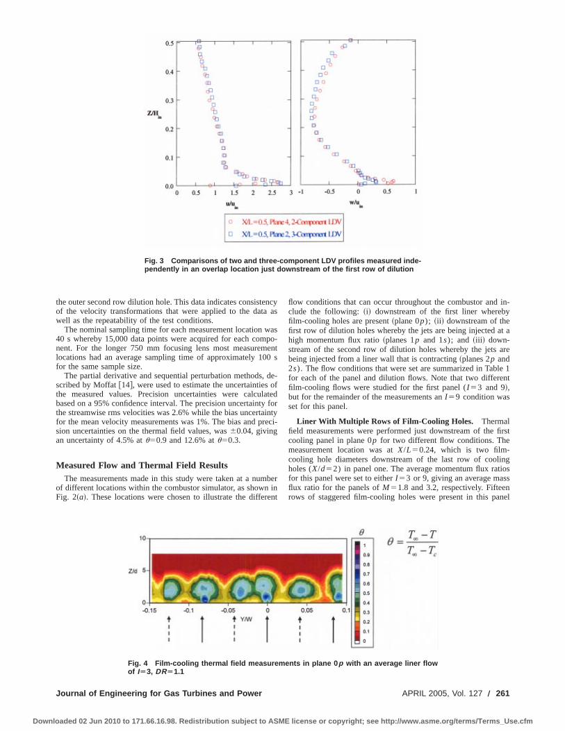
the outer second row dilution hole. This data indicates consistencyof the velocity transformations that were applied to the data aswell as the repeatability of the test conditions.

The nominal sampling time for each measurement location was40 s whereby 15,000 data points were acquired for each compo-nent. For the longer 750 mm focusing lens most measurementlocations had an average sampling time of approximately 100 sfor the same sample size.

The partial derivative and sequential perturbation methods, de-scribed by Moffat@14#, were used to estimate the uncertainties ofthe measured values. Precision uncertainties were calculatedbased on a 95% confidence interval. The precision uncertainty forthe streamwise rms velocities was 2.6% while the bias uncertaintyfor the mean velocity measurements was 1%. The bias and preci-sion uncertainties on the thermal field values, was60.04, givingan uncertainty of 4.5% atu50.9 and 12.6% atu50.3.

Measured Flow and Thermal Field ResultsThe measurements made in this study were taken at a number

of different locations within the combustor simulator, as shown inFig. 2~a!. These locations were chosen to illustrate the different

flow conditions that can occur throughout the combustor and in-clude the following:~i! downstream of the first liner wherebyfilm-cooling holes are present~plane 0p); ~ii ! downstream of thefirst row of dilution holes whereby the jets are being injected at ahigh momentum flux ratio~planes 1p and 1s); and ~iii ! down-stream of the second row of dilution holes whereby the jets arebeing injected from a liner wall that is contracting~planes 2p and2s). The flow conditions that were set are summarized in Table 1for each of the panel and dilution flows. Note that two differentfilm-cooling flows were studied for the first panel (I 53 and 9!,but for the remainder of the measurements anI 59 condition wasset for this panel.

Liner With Multiple Rows of Film-Cooling Holes. Thermalfield measurements were performed just downstream of the firstcooling panel in plane 0p for two different flow conditions. Themeasurement location was atX/L50.24, which is two film-cooling hole diameters downstream of the last row of coolingholes (X/d52) in panel one. The average momentum flux ratiosfor this panel were set to eitherI 53 or 9, giving an average massflux ratio for the panels ofM51.8 and 3.2, respectively. Fifteenrows of staggered film-cooling holes were present in this panel

Fig. 3 Comparisons of two and three-component LDV profiles measured inde-pendently in an overlap location just downstream of the first row of dilution

Fig. 4 Film-cooling thermal field measurements in plane 0 p with an average liner flowof IÄ3, DRÄ1.1



with the hole spacing as that indicated in Fig. 2~b!. While thesemeasurements were conducted, the flow condition for the remain-ing liner panels was set at the same condition as the first panel(I 53 or 9!. Figures 4 and 5 show the measured thermal fields forthe two blowing conditions. The solid arrows represent the loca-tion of the last row of film-cooling holes while the dashed arrowsrepresent the pitch location of the previous row of film-coolingholes. As can be seen by the thermal field measurements, the jetsare periodic in the pitch direction across the panel.

Figures 4 and 5 indicate a cooler jet for the row of jets closestto the measurement plane~solid arrows! as compared with the jetsof the previous row~dashed arrows!. For both flow conditions, thepeak temperature contour representing the coolest fluid is locatedaway from the wall. A separated jet condition is expected giventhe high momentum flux ratio conditions for both cases. The ther-mal field contours for the row of cooling holes closest to themeasurement plane indicate a double-peak with the second peakbeing at a slightly warmer temperature~u50.5! than the primarypeak~u50.7!. The second peak is located just above the coldestpeak and is a remnant of the upstream cooling jet at the samepitchwise alignment. Interestingly, the contour levels for thedashed arrows~upstream row! do not have this double peak,which indicates that given enough streamwise distance the stream-wise jets merge into one cooler core.

Although the conditions through the holes differ by a largeamount of cooling flow, the core of the jets closest to the mea-surement plane~coldest contour! is nominally at the same tem-perature level at this location~u50.7! for both blowing ratios.There are two real differences between these two cases. First, thepenetration depth for theI 59 case appears to be greater than theI 53 case. Second, and more importantly, the fluid temperaturebetween the jets near the wall appears to be cooler for theI 59case~0.25,u,0.35! as compared with theI 53 case~0.15,u,0.2!.

Downstream of the First Row of Dilution Holes. The ther-mal field measured in the streamwise direction through the firstrow of dilution jets is shown in Fig. 6. Recall at this location inthe combustor simulator, the cross-sectional area of the simulatoris the same as that of the entrance. The spanwise distance~Z! isnormalized by this height (H in). The momentum flux ratio for thislarge dilution jet isI 5128 while the mass flux ratio isM512.

The contours in Fig. 6 indicate a penetration distance that isapproximately 18% of the height before the jet trajectory is bentover by the mainstream flow. Upstream of the jet injection, thereis a relatively thick film-cooling layer that is being transportedinto the free stream by the dilution jet. It is also clear that thetemperature gradients are quite high at the jet-mainstream inter-face near the jet injection, while farther away from the wall thetemperature contours are spreading due to the turbulent mixing.The penetration depth of these dilution jets does not extend to thecenterline, which is quite probably a result of the opposing jetsthat are aligned in the pitchwise and streamwise locations.

The solid line shown in Fig. 6 indicates the penetration distancepredicted by the correlation given by Lefebvre@15#. The correla-tion overpredicts the trajectory of the jet and underpredicts thebending of the jet. One plausible reason for the misprediction maybe due to the fact that there is an opposing jet and that thesedilution jets are at very high momentum ratios (I 5128).

Figure 7 shows the measured thermal field for a plane thatextends in the pitchwise direction downstream of the first row ofdilution jets at a location that is two film-cooling hole diametersdownstream of the last row of cooling holes in the second liner.This location is 1.3 hole diameters (X51.3D1) downstream of thedilution hole whereby this distance is measured from the holecenterline. This larger plane was taken to illustrate the pitchwisesymmetry of the dilution flow. These thermal fields indicate thatthe coolant from the dilution jets has been transported to a regionslightly offset from the center of the two lobes of the kidney-shaped vortex. It is important to recognize that the distance be-

Fig. 5 Film-cooling thermal field measurements in plane 0 pwith an average liner flow of IÄ9, DRÄ1.1

Fig. 6 Thermal field contours in a streamwise plane through afirst row dilution hole „plane 1 s… with Lefebvre’s †15‡ jet pen-etration correlation

Fig. 7 Thermal field contours in plane 1 p



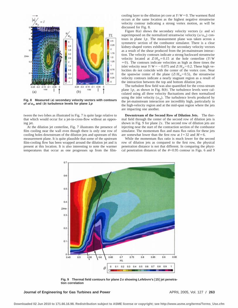
tween the two lobes as illustrated in Fig. 7 is quite large relative tothat which would occur for a jet-in-cross-flow without an oppos-ing jet.

At the dilution jet centerline, Fig. 7 illustrates the presence offilm cooling near the wall even though there is only one row ofcooling holes downstream of the dilution jets and upstream of thismeasurement plane. It is quite plausible that some of the upstreamfilm-cooling flow has been wrapped around the dilution jet and ispresent at this location. It is also interesting to note the warmertemperatures that occur as one progresses up from the film-

cooling layer to the dilution jet core atY/W50. The warmest fluidoccurs at the same location as the highest negative streamwisevelocity contour indicating a strong vortex motion, as will bediscussed for Fig. 8.

Figure 8~a! shows the secondary velocity vectors (v and w!superimposed on the normalized streamwise velocity (u/uin) con-tours in plane 1p. The measurement plane was taken across asymmetric section of the combustor simulator. There is a clearkidney-shaped vortex exhibited by the secondary velocity vectorsas a result of the shear produced from the jet-mainstream interac-tion. The velocity contours indicate a strong backward streamwisevelocity located atZ/H in50.15 at the hole centerline (Y/W50). The contours indicate velocities as high as three times theinlet velocity nearY/W520.075 andZ/H in50.2. These high ve-locities do not coincide with the center of the vortex core. Nearthe spanwise center of the plane (Z/H in50.5), the streamwisevelocity contours indicate a nearly stagnant region as a result ofthe interaction between the top and bottom dilution jets.

The turbulent flow field was also quantified for the cross-streamplane 1p, as shown in Fig. 8~b!. The turbulence levels were cal-culated using all three velocity fluctuations and then normalizedusing the inlet velocity (uin). The turbulence levels produced bythe jet-mainstream interaction are incredibly high, particularly inthe high-velocity region and at the mid-span region where the jetsare impacting one another.

Downstream of the Second Row of Dilution Jets. The ther-mal field through the center of the second row of dilution jets isshown in Fig. 9 for plane 2s. The second row of dilution jets areinjecting near the start of the contraction section of the combustorsimulator. The momentum flux and mass flux ratios for these jetsare somewhat lower than the first row atI 532 andM56.

While the momentum flux ratio is much lower for the secondrow of dilution jets as compared to the first row, the physicalpenetration distance is not that different. In comparing the physi-cal penetration distances of theu50.95 contour in Figs. 6 and 9

Fig. 8 Measured „a… secondary velocity vectors with contoursof u Õu in and „b… turbulence levels for plane 1 p

Fig. 9 Thermal field contours for plane 2 s showing Lefebvre’s †15‡ jet penetra-tion correlation



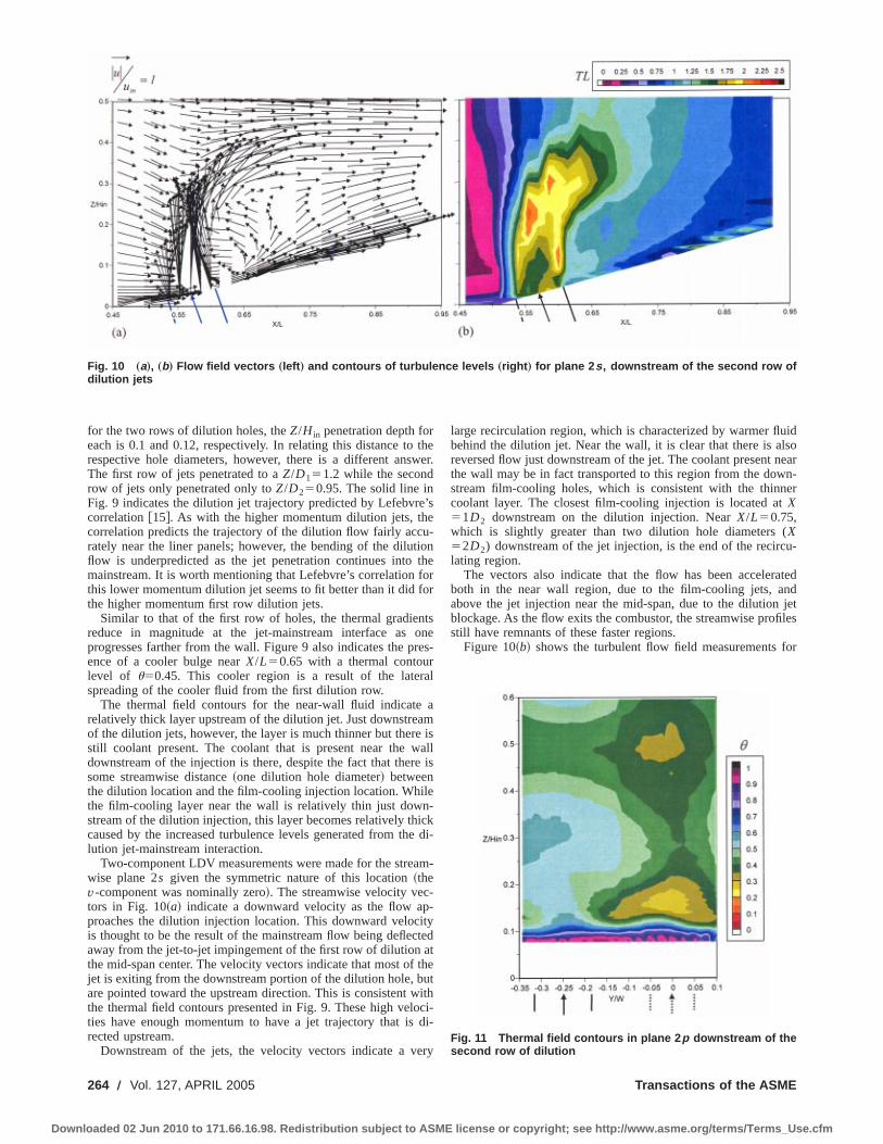
for the two rows of dilution holes, theZ/H in penetration depth foreach is 0.1 and 0.12, respectively. In relating this distance to therespective hole diameters, however, there is a different answer.The first row of jets penetrated to aZ/D151.2 while the secondrow of jets only penetrated only toZ/D250.95. The solid line inFig. 9 indicates the dilution jet trajectory predicted by Lefebvre’scorrelation@15#. As with the higher momentum dilution jets, thecorrelation predicts the trajectory of the dilution flow fairly accu-rately near the liner panels; however, the bending of the dilutionflow is underpredicted as the jet penetration continues into themainstream. It is worth mentioning that Lefebvre’s correlation forthis lower momentum dilution jet seems to fit better than it did forthe higher momentum first row dilution jets.

Similar to that of the first row of holes, the thermal gradientsreduce in magnitude at the jet-mainstream interface as oneprogresses farther from the wall. Figure 9 also indicates the pres-ence of a cooler bulge nearX/L50.65 with a thermal contourlevel of u50.45. This cooler region is a result of the lateralspreading of the cooler fluid from the first dilution row.

The thermal field contours for the near-wall fluid indicate arelatively thick layer upstream of the dilution jet. Just downstreamof the dilution jets, however, the layer is much thinner but there isstill coolant present. The coolant that is present near the walldownstream of the injection is there, despite the fact that there issome streamwise distance~one dilution hole diameter! betweenthe dilution location and the film-cooling injection location. Whilethe film-cooling layer near the wall is relatively thin just down-stream of the dilution injection, this layer becomes relatively thickcaused by the increased turbulence levels generated from the di-lution jet-mainstream interaction.

Two-component LDV measurements were made for the stream-wise plane 2s given the symmetric nature of this location~thev-component was nominally zero!. The streamwise velocity vec-tors in Fig. 10~a! indicate a downward velocity as the flow ap-proaches the dilution injection location. This downward velocityis thought to be the result of the mainstream flow being deflectedaway from the jet-to-jet impingement of the first row of dilution atthe mid-span center. The velocity vectors indicate that most of thejet is exiting from the downstream portion of the dilution hole, butare pointed toward the upstream direction. This is consistent withthe thermal field contours presented in Fig. 9. These high veloci-ties have enough momentum to have a jet trajectory that is di-rected upstream.

Downstream of the jets, the velocity vectors indicate a very

large recirculation region, which is characterized by warmer fluidbehind the dilution jet. Near the wall, it is clear that there is alsoreversed flow just downstream of the jet. The coolant present nearthe wall may be in fact transported to this region from the down-stream film-cooling holes, which is consistent with the thinnercoolant layer. The closest film-cooling injection is located atX51D2 downstream on the dilution injection. NearX/L50.75,which is slightly greater than two dilution hole diameters (X52D2) downstream of the jet injection, is the end of the recircu-lating region.

The vectors also indicate that the flow has been acceleratedboth in the near wall region, due to the film-cooling jets, andabove the jet injection near the mid-span, due to the dilution jetblockage. As the flow exits the combustor, the streamwise profilesstill have remnants of these faster regions.

Figure 10~b! shows the turbulent flow field measurements for

Fig. 10 „a…, „b… Flow field vectors „left … and contours of turbulence levels „right … for plane 2 s , downstream of the second row ofdilution jets

Fig. 11 Thermal field contours in plane 2 p downstream of thesecond row of dilution



plane 2s. The peak turbulence levels, which occur at the jet-mainstream interface, are 2.2 times greater than the inlet velocity.It is important to recognize that at the dilution jet injection loca-tion, the mass-averaged velocity is 2.7 times that of the inlet ve-locity ~indicated in Table 1! as a result of the mass flow injectionfrom the first row of dilution jets and the film-cooling addition.The jet turbulence itself is relatively lower than that occurring asthe jet interacts with the mainstream flow. In the jet recirculatingregion, the turbulence levels are very high, considering the factthat the local flow velocities in this region are relatively low. Thenear-wall turbulence that is generated is also relatively high due to

the film-cooling injection. As the flow exits the combustor, thelevels relative to the local exit velocity are on the order of 20%.

Figure 11 shows the thermal field contours downstream of thesecond row of dilution jets~plane 2p) for a region larger than thesymmetric locations to illustrate the thermal field symmetry. Notethat both jets inject to approximately the same spanwise locationrelative to the mid-span. The dashed lines represent the spanwiseinjection location of the first row of dilution holes while the solidlines represent the second row of dilution holes. At this stream-wise location, which is one dilution hole diameter downstream ofthe second row of dilution holes (X51D2), the coldest tempera-ture contour for the dilution flow isu50.55 located atY/W520.25 at aboutZ/H in50.3. The warmer fluid shown nearY/W50 at Z/H in50.15 is a remnant of the warm fluid that is trappedin the recirculating region downstream of the first row of dilutionjets. A similarly warm region is located just above that region nearthe mid-span, which is a result of warmer fluid penetrating be-tween the opposing first row of dilution jets.

Figure 12 shows the secondary velocity vectors superimposedon the streamwise velocity contours at the same plane 2p onlywith a smaller measurement region as compared with Fig. 10. Atthis location, it is clear that there is no evidence from the vectorsas to a strong kidney vortex as there was in the case of the firstrow of dilution holes. The high turbulence levels, as will be illus-trated in the upcoming figures, have caused a reduction in theswirl velocities. There is a strong upward flow that is a result ofthe contraction section of the combustor. The streamwise veloci-ties indicate that the flow has accelerated to about three times theinlet velocity near the mid-span. At a span of approximately 25%of the inlet height, there is a near zero velocity just downstream ofthe dilution holes, similar to that of the first row of dilution jets,which is caused by the jet blockage. To illustrate the anisotropicbehavior of the turbulence of the dilution jets, Figs. 13~a!–13~c!show the measured fluctuations for all three velocity components.As can be seen, all three contour plots illustrate a very differentbehavior. The highest fluctuation levels in this plane are 1.75times that of the inlet velocity. It is important to remember that atthis location the mass-averaged velocity is 2.7 times faster thanthe inlet velocity, which still translates to average rms levels that

Fig. 12 Secondary velocity vectors with contours of thestreamwise velocities in plane 2 p

Fig. 13 „a…–„c… Contours of the rms fluctuations for the flow in plane 2 p



are 0.65 times the local mass averaged velocity. The peak stream-wise velocity fluctuations occurs atZ/H in50.3 and Y/W520.25, which coincides with the core of the jet~as indicated bythe thermal field contours in Fig. 11!. The peak spanwise velocityfluctuations (v rms), which are slightly higher at 2.1 times the inletvelocity, occur near the liner wall just below the core of the jet.Similar to the streamwise fluctuations, the peak spanwise fluctua-tions occur at the core of the jet and above.

The turbulence levels for the pitchwise plane, which is a com-bination of the fluctuations for all three velocity components, isshown in Fig. 14 for plane 2p. For the second row of injection(Y/W520.25), the peak level coincides with a region slightlyhigher than the core of the jet. While the levels are much lower,the peak region for the first row of dilution jets coincides moreclosely with the mid-span.

Conclusions and RecommendationsThe results of this study indicate the complexity of the flow that

occurs in a typical aeroengine combustor. While these results wereacquired with a nonreacting flow, it is important to have a place tobegin when it comes to making comparisons with computationalpredictions. In particular, it is important that we are able to under-stand how the interactions take place between rows of dilution jetsand liner film-cooling. The resolution of the measured data pre-sented in this paper was only made possible through scaling up ofa combustor.

The measurements indicate the dominance of the dilution jetson the flow and thermal fields. Kidney-shaped thermal fields werepresent as the result of the dilution jet-mainstream interaction.One notable feature was the spreading of the two kidney lobesthat resulted from the impacting of the jets. Downstream of thedilution jet injection, there was a large recirculating region thattransported warm fluid into the region just downstream of theinjection. While the near-wall film of coolant is much thinner justdownstream of the dilution holes, there is still coolant present. Todetermine whether the coolant was transported by vortices wrap-ping around the dilution jet or transported by the reverse flowdownstream of the dilution jet is not known at this time. Furtherwork needs to be conducted to determine the true mechanism thatis important for combustor cooling strategies.

The turbulence levels were measured to be extremely highthroughout the combustor as well as highly anisotropic. It is clearas to why current two-equation turbulence models underpredict

these turbulence levels given the model assumptions of isotropicturbulence. The exit turbulence levels, based on the local averageexit velocity were 20%.

Further studies need to be done to evaluate cooling schemesalong the liner wall and ensure good coverage near the dilutionholes. More detailed measurements are needed near the dilutionholes to evaluate these cooling schemes. Given the results pre-sented in this paper, it is possible to compare computational pre-dictions with measured flow and thermal fields.

AcknowledgmentsThe authors gratefully acknowledge United Technologies—

Pratt and Whitney for their support of this work.

Nomenclature

ALP 5 air loading parameter, ALP5P01.75ArefD ref

0.75eT/300/m,Lefebvre@15#

d 5 film cooling hole diameterD1 , D2 5 dilution hole diameters for first and second rows

H in 5 combustor inlet heightI 5 momentum flux ratio,I 5rcUc

2/r`U`2

L 5 film cooling hole length, combustor simulatorlength

m 5 mass flow rateM 5 mass flux ratio,M5rcUc /r`U`P 5 vane pitch

Ss , Sp 5 streamwise, pitchwise film cooling hole spacingT 5 temperature

TL 5 turbulence level, TL50.33(urms2 1v rms

2 1wrms2 )0.5/uin

~3-comp.! and TL50.5(urms2 1wrms

2 )0.5/uin ~2-comp.!u, v, w 5 local, mean velocity componentsX, Y, Z 5 coordinate system shown in Fig. 2~a!

W 5 combustor inlet width

Greek

r 5 densityn 5 kinematic viscosityu 5 nondimensional temperature,u5(T`2T)/(T`2Tc)

Subscripts

ave 5 spatial averagerms 5 root mean square

` 5 free-stream conditions~primary flow!c 5 coolant conditions~secondary flow!

References@1# Barringer, M. D., 2001, ‘‘Design and Benchmarking of a Combustor Simulator

Relevant to Gas Turbine Engines,’’ Master’s thesis, Virginia Polytechnic Insti-tute and State University.

@2# Zimmerman, D. R., 1979, ‘‘Laser Anemometer Measurements at the Exit of aT63-C20 Combustor,’’ National Aeronautics and Space Administration, NASALewis Research Center, Contract No. NAS 3-21267.

@3# Goldstein, R. J., 1983, ‘‘Velocity and Turbulence Measurements in Combus-tion Systems,’’ Exp. Fluids,1, pp. 93–99.

@4# Moss, R. W., 1992, ‘‘The Effects of Turbulence Length Scale on Heat Trans-fer,’’ Ph.D. dissertation, Department of Engineering Science, University ofOxford, Report No. OUEL 1924/92.

@5# Cameron, C., Brouwer, J., Wood, C., and Samuelson, G., 1989, ‘‘A DetailedCharacterization of the Velocity and Thermal Fields in a Model Can Combus-tor With Wall Jet Injection,’’ ASME J. Eng. Gas Turbines Power,111, pp.31–35.

@6# Gulati, A., Tolpadi, A., VanDuesen, G., and Burrus, D., 1995, ‘‘Effect of Di-lution Air on the Scalar Flowfield at Combustor Sector Exit,’’ J. Propul. Power,11, pp. 1162–1169.

@7# Holdeman, J. D., 1993, ‘‘Mixing of Multiple Jets With a Confined SubsonicCrossflow,’’ Prog. Energy Combust. Sci.,19, pp. 31–70.

@8# Stitzel, S. M., 2001, ‘‘Flow Field Computations of Combustor-Turbine Inter-action in a Gas Turbine Engine,’’ Master’s thesis, Virginia Polytechnic Instituteand State University.

@9# Malecki, R., Rhie, C., McKinney, R., Ouyang, H., Syed, S., Colket, M., andMadhabushi, R., 2001, ‘‘Application of an Advanced CFD-Based Analysis

Fig. 14 Contours of turbulence levels in plane 2 p



System to the PW6000 Combustor to Optimize Exit TemperatureDistribution—Part I: Description and Validation of the Analysis Tool,’’ ASMEPaper No. 2001-GT-0062.

@10# Goebel, S., Abauf, N., Lovett, J., and Lee, C., 1993, ‘‘Measurements of Com-bustor Velocity and Turbulence Profiles,’’ ASME Paper No. 93-GT-228.

@11# Stevens, S. J., and Carotte, J. F., 1990, ‘‘Experimental Studies of CombustorDilution Zone Aerodynamics, Part I: Mean Flowfields,’’ J. Propul. Power,6,pp. 297–304.

@12# Liou, T. M., and Wu, Y. Y., 1992, ‘‘LDV Measurements of the Flowfield in a

Simulated Combustor With Axial and Side Inlets,’’ Exp. Therm. Fluid Sci.,5,pp. 401–409.

@13# Barringer, M. D., Richard, O. T., Walter, J. P., Stitzel, S. M., and Thole, K. A.,2001, ‘‘Flow Field Simulations of a Gas Turbine Combustor,’’ ASME J. Tur-bomach.,124, pp. 508–516.

@14# Moffat, J. R., 1988, ‘‘Describing the Uncertainties in Experimental Results,’’Exp. Therm. Fluid Sci.,1, pp. 3–17.

@15# Lefebvre, A. H., 1999,Gas Turbine Combustion, Taylor & Francis, Philadel-phia, PA.



Iain D. J. Dupere

Ann P. Dowling

Department of Engineering,University of Cambridge,

Cambridge CB2 1PZ, United Kingdom

The Use of Helmholtz Resonatorsin a Practical CombustorThe drive to reduce emissions has led to the development of lean premixed combustors.However, lean premixed combustion is often associated with combustion oscillationswhich can be so severe that they can cause structural damage to the engine. Since theassociated frequencies are typically of the order of hundreds of Hertz, there is a need fora compact device to absorb the noise which drives the oscillation. Helmholtz resonatorsare commonly used as absorbers of incident acoustic power. In addition they are relativelycompact. However, their use in combustors creates practical issues, such as placementwithin the chamber, neck length, and cooling, which need to be addressed. In this paperwe consider these practical problems and describe how to overcome them in a realcombustor.@DOI: 10.1115/1.1806838#

1 IntroductionLow NOx combustion can be achieved using lean premixed

systems. Here the temperature is more evenly distributed and thepeak temperature lower, leading to low NOx production. Unfortu-nately, low NOx combustors are often associated with combustioninstabilities which can be so severe that structural damage to theengine occurs. Helmholtz resonators are commonly used to dampincident acoustic waves in a number of applications~see, for ex-ample@1–6#!. Helmholtz resonators have the advantage that theyrequire a relatively small volume to damp oscillations at the rela-tively low frequencies found in combustion systems and thus pro-vide a useful damping mechanism for combustion oscillation@1,3#. In order to control oscillations, they must communicate withthe combustor itself. This places practical constraints upon theirdesign, limiting their performance.

The need to incorporate the Helmholtz resonator so that it cancommunicate with the combustion chamber places strong con-straints upon the aperture size, neck length, and volume of theHelmholtz resonator. In particular, the neck length needs to berelatively long and this results in a compromise between the ab-sorption obtained at the peak and the frequency range over whichsignificant absorption is obtained. A systematic approach forchoosing the parameters is developed and described in this paper.We also consider the case of a neck which is long in comparisonwith the wavelength and its practical use in an engine.

We consider two types of configuration: no mean flow and witha mean flow. The mean flow may be either tangential across theface of the aperture or be like a cooling flow through the aperture.A combination of a cooling flow with a tangential flow is alsopossible. The no flow case is associated with nonlinear absorptionof sound which depends upon the amplitude of the neck pressure,which in turn depends upon the incident acoustic energy, the com-bustor geometry, and the location of the neck. We describe thisregime by using a model developed by Cummings@7# for thenonlinear behavior of an aperture and compare our results with anexperiment, obtaining good agreement.

In the presence of a mean flow the absorption coefficient islinear ~i.e., independent of neck pressure! and associated with theconvection of unsteadily shed vorticity from the neck of the reso-nator. However, it still depends upon the combustor geometry andthe location of the neck. Both tangential and cooling flows aremodeled by using a Rayleigh conductivity first derived by Howe

and his co-workers for each flow regime separately. In the pres-ence of a tangential mean flow the convecting vorticity can alsointeract with the downstream edge of the aperture and generatesound. This can be overcome by rounding the downstream edge orby combining the tangential flow with cooling through the neck.Finally we draw some conclusions.

2 Practical Helmholtz Resonators

2.1 Introduction. Helmholtz resonators consist of a cham-ber and a neck as illustrated in Fig. 1. Oscillation occurs when themass of gas in the neck vibrates against the gas in the chamber.They can simply consist of a perforation in a plate above thechamber@8#, the end correction acting as the neck. In the absenceof a mean flow, absorption of incident sound is related to thenonlinear viscous damping of the flow in the neck region, and theabsorption is only significant near resonance. This mechanism ul-timately ensures that the neck velocity remains finite. Further-more, a significant proportion of the incident sound energy willonly be absorbed at high acoustic amplitudes. This phenomenoncan be modeled by an appropriate nonlinear model such as pro-posed by Cummings@7#. A similar model applied to Helmholtzresonators was successfully used by Bellucci et al.@1#.

In the presence of a mean flow incident acoustic waves causeunsteady vortex waves to be shed at the edges of the aperturewhich is swept away by the mean flow. This convecting vorticityacts as a sink to the incident sound near the upstream edge.

In this paper, we consider the acoustic response of an idealizedsystem consisting of a resonator chamber connected to a pipecontaining incident sound energy via an aperture. The problemcan be separated into three features: the acoustic properties of thecombustion chamber, the local absorption due to a finite pressuredifference between the pipe and the Helmholtz resonator chamber,and the enhancement of the absorption due to resonance. Whenthe neck of the Helmholtz resonator consists of an aperture in apipe wall connecting it to the resonator chamber, the local absorp-tion is characterized by the Rayleigh conductivity. This was de-rived by Howe and his co-workers for mean flow both through theaperture@9# and for tangential flow across it@10#. A correction isrequired for the finite wall thickness. Howe’s model has been usedextensively in the literature to model the interaction betweensound and mean flow in a wide variety of applications, includingHelmholtz resonators@2,4–6,11–17#.

In a practical system, space will often prevent Helmholtz reso-nators from being attached to the region of interest via a shortneck. We consider, therefore, practical resonators with notablephysical lengths. Initially the Rayleigh conductivity for the neck isassumed to be a known complex quantityk5g2 id.




Consider the system illustrated in Fig. 1. This consists of aninfinitely long pipe of cross-sectional areaS1 , to which a Helm-holtz resonator chamber is attached atx50 via a neck of effectivelength l and areaS2 . An incident sound wave, whose complexamplitude isA at x50, propagates along the pipe from left to rightfrom x52` to x50. A second incident acoustic wave, with com-plex amplitudeD, propagates from right to left fromx51` tox50. At x50, a right propagating wave, of complex amplitudeC,is generated by the combination of transmission of waveA andreflection of waveD. Similarly a left propagating wave, of com-plex amplitudeB, is generated in the left-hand part of the pipe. Inaddition unsteady flow of speeduHR and mass flowmHR8 entersthe Helmholtz resonator through the neck and a low Mach number~which may be zero! mean flow flows along the pipe from left toright. We neglect viscous effects, except at the opening.

We begin by equating the change of mass inside the chamber tothe unsteady neck flow:

V]r28

]t5 rS2uHR8 ,⇒ ivVr285 rS2uHR8 (1)

for harmonic excitation of angular frequencyv. If we furtherassume that the unsteady flow inside the resonator chamber isisentropic, then we can relate the fluctuating resonator chamberpressure,p28 , to the fluctuating density,r28 , and hence to the neckvelocity via Eq.~1! to give

p285c22

ruHR8 S2

ivV(2)

The acoustic pressure waves on either side of the resonator arerelated~from energy or momentum considerations! by

A~11M !1B~12M !5C~11M !2D~12M ! (3)

The behavior of the neck is linear in the presence of a meanflow, but nonlinear with no mean flow. We consider the nonlinearbehavior first.

2.1.1 Non-Linear Theory. Following Cummings @7# theacoustic velocity,u18 is given by

p182p285 l]u18

]t1

c

2u18uu18u (4)

5 iv lu181c

2u18uu18u (5)

wherel is the effective length of the Helmholtz resonator neck andc is the discharge coefficient describing the nonlinear behavior ofthe neck. Both the effective neck length,l, and the discharge co-efficient, c, are determined experimentally. Substituting forp28into equation~5!,

p185u18i S v l 2c2rS

vV D1c

2u18uu18u (6)

For low amplitudes, the nonlinear real part of the right-hand sideof Eq. ~6! is small and so little absorption of sound energy occurs.The imaginary part then gives resonance at the frequency given byclassical theory.

Nonlinear equation~6! is solved numerically for the acousticvelocity, u18 , for a given neck pressure amplitude,p18 , which canalso be related to the downstream wavesC andD using Eq.~3!.u18 can be related to the incident acoustic velocities by consideringthe conservation of acoustic mass flow, i.e.,

rA1S A2B

r c D5 rSu181 rA1S C2D

r c D (7)

Equation~7! together with Eq.~3! can be solved to give the inci-dent and reflected wavesA andB.

Equations~3! and ~7! together with equation~6! are used topredict the four acoustic waves,A, B, C and D, for a range ofsound pressure levels. We present our results in terms of the ab-sorption coefficient, defined as the fraction of incident energywhich is absorbed, since we are interested in absorption,

i.e., D512S uBu21uCu2

uAu21uDu2D (8)

Sample results are shown in Fig. 2 which is for a neck pressureof 165 dB which also shows comparison with experimental mea-surements. The experimental arrangement is described in the Ap-pendix. The agreement between the theory and the experiment isgood. Although much of the literature on Helmholtz resonators isconcerned with predicting the resonant frequency~see, for ex-ample, Chanaud@11,12#!, a number of other studies have alsofound good agreement with experiment for the amplitude response@1,4–6,13–17#. At the peak 65% of the incident sound is ab-sorbed. Even at 135 dB the peak absorption is between 50% and60% depending upon the configuration. However, the absorptioncharacteristics include a distinct minimum. This results from apressure node at the neck of the Helmholtz resonator. This has twoeffects. The first, and most obvious, is that the sound pressurelevels found in practice will be low near this frequency. Second,when the unsteady pressures nearly cancel at the neck of the reso-nator, specific neck pressure levels can only be achieved withlarge incident sound waves. The unsteady velocity into the reso-nator, u18 , however, is solely a function of this neck pressureamplitude@see Eq.~6!# and so will not be affected by the presenceof the node. Thus the actual amount of energy absorbed is purelya function of the neck pressure and the behavior of the resonator.The incident acoustic energy, and thus the fraction of energywhich is absorbed, however, also depend upon the amplitude of

Fig. 1 An illustration of a real Helmholtz resonator attached to a pipe



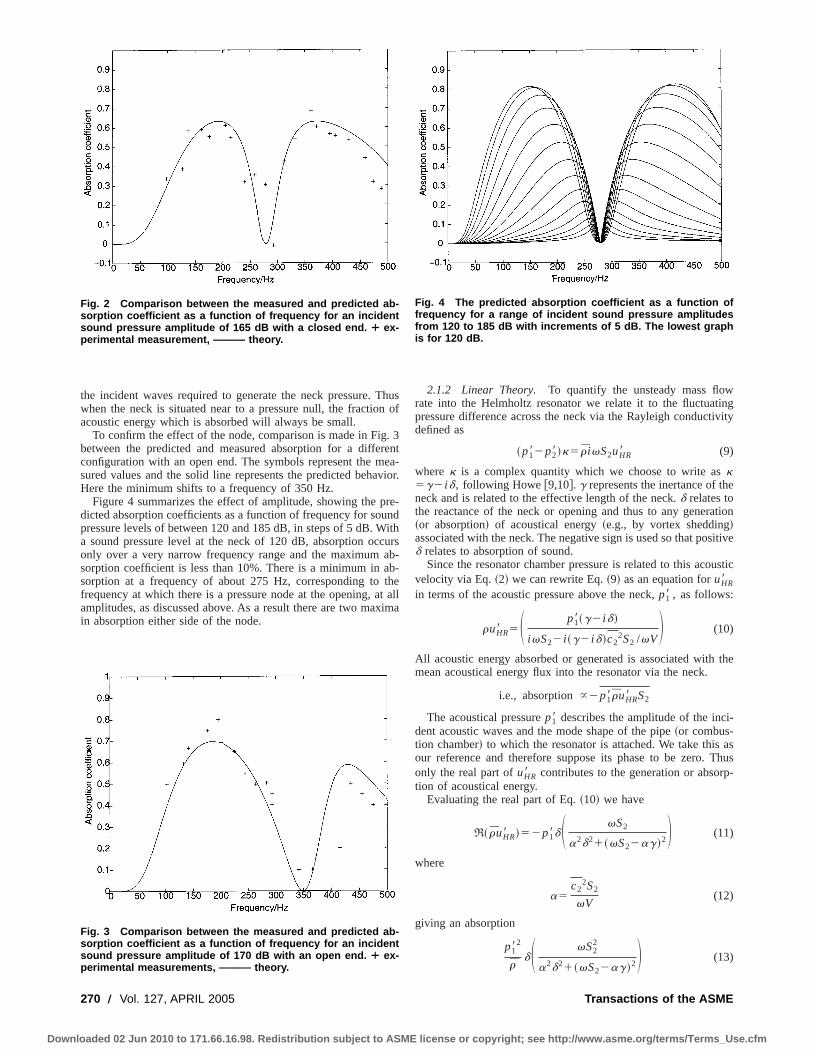
the incident waves required to generate the neck pressure. Thuswhen the neck is situated near to a pressure null, the fraction ofacoustic energy which is absorbed will always be small.

To confirm the effect of the node, comparison is made in Fig. 3between the predicted and measured absorption for a differentconfiguration with an open end. The symbols represent the mea-sured values and the solid line represents the predicted behavior.Here the minimum shifts to a frequency of 350 Hz.

Figure 4 summarizes the effect of amplitude, showing the pre-dicted absorption coefficients as a function of frequency for soundpressure levels of between 120 and 185 dB, in steps of 5 dB. Witha sound pressure level at the neck of 120 dB, absorption occursonly over a very narrow frequency range and the maximum ab-sorption coefficient is less than 10%. There is a minimum in ab-sorption at a frequency of about 275 Hz, corresponding to thefrequency at which there is a pressure node at the opening, at allamplitudes, as discussed above. As a result there are two maximain absorption either side of the node.

2.1.2 Linear Theory. To quantify the unsteady mass flowrate into the Helmholtz resonator we relate it to the fluctuatingpressure difference across the neck via the Rayleigh conductivitydefined as

~p182p28!k5 r ivS2uHR8 (9)

where k is a complex quantity which we choose to write ask5g2 id, following Howe@9,10#. g represents the inertance of theneck and is related to the effective length of the neck.d relates tothe reactance of the neck or opening and thus to any generation~or absorption! of acoustical energy~e.g., by vortex shedding!associated with the neck. The negative sign is used so that positived relates to absorption of sound.

Since the resonator chamber pressure is related to this acousticvelocity via Eq.~2! we can rewrite Eq.~9! as an equation foruHR8in terms of the acoustic pressure above the neck,p18 , as follows:

ruHR8 5S p18~g2 id!

ivS22 i ~g2 id!c22S2 /vV

D (10)

All acoustic energy absorbed or generated is associated with themean acoustical energy flux into the resonator via the neck.

i.e., absorption}2p18ruHR8 S2

The acoustical pressurep18 describes the amplitude of the inci-dent acoustic waves and the mode shape of the pipe~or combus-tion chamber! to which the resonator is attached. We take this asour reference and therefore suppose its phase to be zero. Thusonly the real part ofuHR8 contributes to the generation or absorp-tion of acoustical energy.

Evaluating the real part of Eq.~10! we have

R~ ruHR8 !52p18dS vS2

a2d21~vS22ag!2D (11)

where

a5c2

2S2

vV(12)

giving an absorption

p182

rdS vS2

2

a2d21~vS22ag!2D (13)

Fig. 2 Comparison between the measured and predicted ab-sorption coefficient as a function of frequency for an incidentsound pressure amplitude of 165 dB with a closed end. ¿ ex-perimental measurement, ——— theory.

Fig. 3 Comparison between the measured and predicted ab-sorption coefficient as a function of frequency for an incidentsound pressure amplitude of 170 dB with an open end. ¿ ex-perimental measurements, ——— theory.

Fig. 4 The predicted absorption coefficient as a function offrequency for a range of incident sound pressure amplitudesfrom 120 to 185 dB with increments of 5 dB. The lowest graphis for 120 dB.



Comparison between theory and experimental measurements ofthe absorption obtained by this mechanism is shown in Fig. 5 fora sample cross flow Mach number of 0.04. Here the Rayleighconductivity used for the predictions is taken from Howe’s model@10#. Similar results have also been obtained for a cooling flowand a combination of a cooling flow and a cross flow~also fromHowe’s model! and were presented in a previous paper@18#. Theabsorption is shown for a variety of amplitudes of unsteady pres-sure at the neck and shown to have little effect on the overallabsorption, which is reasonably high here. As before the minimumabsorption occurs when the resonator neck is near a pipe node.Notice that at this temperature and with a relatively short neck theabsorption is high and occurs over a broad range of frequencies.This ceases to be the case at higher temperatures and with longnecks as would be required if it were to be implemented in a realcombustion chamber. The practical implications of this are dis-cussed below.

2.2 Discussion. For low amplitude sound waves in the ab-sence of a mean flow, the Rayleigh conductivity of the neck ispurely imaginary~i.e., d50!, leading to the denominator of Eq.~13! being purely imaginary and becomes zero when

vS25ag, i.e., when v5c2Ag

V(14)

Since g5S2 / l e f f ective , the familiar formula for the resonantfrequency of a Helmholtz resonator is recovered. Here the un-steady flow velocity into the Helmholtz resonator is large, andnonlinear effects become important. This limits the velocity andleads to some sound absorption, as described above. In the pres-ence of a mean flow, however,d has a nonzero value, leading toabsorption away from resonance. Since the imaginary part of thedenominator in Eq.~13! can still be set to zero at the frequencydefined by Eq.~14!, this might be supposed to enhance the ab-sorption for modestd. When this occurs Eq.~13! becomes

absorption5p18

2

r S g3/2V1/2

dc2D (15)

sincevS25ag. It is clear from Eq.~15! that the absorption at theconventional resonance frequency is inversely proportional tod.This occurs becaused describes the local absorption of the neckirrespective of its acoustics environment. For very small but finited, there is a little absorption at most frequencies. Near resonance,

however, the large neck velocities enhance the absorption. Asdincreases, noticeable absorption occurs over a broader range offrequencies. However, at resonance the effect of the increased‘‘local’’ absorption is to suppress resonance, reducing the peakabsorption. This is illustrated in Fig. 6, which shows the variationin absorption coefficient of one Helmholtz resonator at three dif-ferent flow conditions. All configurations are for mean flowthrough the aperture. The volume of the resonator chamber ischosen to give peak absorption at 500 Hz for the lowest neckvelocity, which has the greatest peak absorption. The Rayleighconductivity used in the calculations to produce Fig. 6 is fromHowe et al.’s solution for an aperture in an infinitely thin plate@10#, as before, with a correction applied to account for the physi-cal length of the neck. Since the Rayleigh conductivity, andg inparticular, is a function of Strouhal number and hence frequency,the frequency at which peak absorption occurs varies slightly be-tween the three configurations. This has not been compensated forhere since the magnitude of the absorption depends upona8,which is itself a function of the volume. Nevertheless, it is clearfrom Fig. 6 that increasingd gives absorption over a broaderrange of frequencies, but at the expense of peak absorption. Thishas strong consequences for the use of Helmholtz resonators incombustion systems. If the resonators are to have a significanteffect in damping the oscillations, then it is essential that they areattached to the combustion chamber itself. However, the high tem-peratures in the combustion chamber result in complicated linersand a cooling system. As a result the neck of the Helmholtz reso-nator will often have to be several centimeters long. The dampingdescribed by Fig. 6 suggests that this limits the overall perfor-mance of the resonator, leaving the designer to choose the balancebetween the maximum absorption achieved and the frequencyrange over which this absorption occurs. Unfortunately, the cur-rent understanding of the instability does not presently give anapriori estimate of the amount of absorption required.

The other factors which appear in Eq.~15! are g; the soundspeed in the Helmholtz resonator chamber,c2; the volume of theHelmholtz resonator chamber,V; the mean density,r; and theacoustic pressure above the aperture,p18 . g describes the inertanceof the aperture per unit area and is large for large radius and shortneck length. In common withd, g is proportional to the aperturediameter. Sinceg has a higher power in Eq.~15! than d, theabsorption increases with aperture size. The absorption is in-versely proportional to the sound speed and so we require a smallsound speed, and thus a low temperature in the Helmholtz reso-nator chamber for high absorption. The volume of the resonatorchamber,V, is constrained to give resonance at the desired fre-

Fig. 5 The variation of acoustic absorption coefficient withfrequency for a Helmholtz resonator with a sound pressurelevel at the neck opening of 155 dB and in the presence of amean pipe flow Mach number of 0.04. ——— theory, Œ ¯ 145 dB,Ã–"– 150 dB, ¿ ——— – 155 dB.

Fig. 6 A graph showing the variation of absorption coefficientwith frequency for three different mean aperture velocities, fora practical Helmholtz resonator with a finite neck length



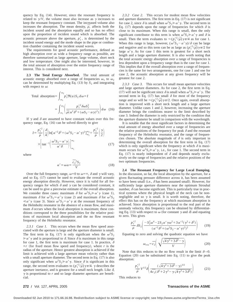
quency by Eq.~14!. However, since the resonant frequency isrelated tog/V, the volume must also increase asg increases tokeep the resonant frequency constant. The increased volume alsoincreases the absorption. The mean density,r, affects both theincident sound and the absorption equally and so has no effectupon the proportion of incident sound which is absorbed. Theacoustic pressure above the aperture,p18 , is determined by theincident sound energy and the mode shape in the pipe or combus-tion chamber containing the incident sound waves.

The requirements for good acoustic performance, defined ashigh absorption over as wide a frequency range as possible, aretherefore summarized as large aperture, large volume, short neckand low temperature. One might also be interested, however, inthe total amount of absorption over the entire frequency range ofinterest. This is considered next.

2.3 The Total Energy Absorbed. The total amount ofacoustic energy absorbed over a range of frequenciesv1 to v2can be determined by multiplying Eq.~13! by S2 and integratingwith respect tov:

Total absorption5Ev1

v2

p18R~u!S2 dv5I

5Ev1

v2S p182dvS2

2

r~a2d21~vS22ag!2!D dv (16)

If g and d are assumed to have constant values over this fre-quency range, Eq.~16! can be solved directly to give

I 5p18

2

r S d

4D ln@a82d21~v2S22a8g!2#v1

v21p18

2

r S g

2D3F tan21S v2S22a8g

a8d D Gv1

v2

(17)

where

a85va5c2

2S2

V(18)

Over the full frequency range,v50 to v5`, d andg will vary,and so Eq.~17! cannot be used to evaluate the overall acousticenergy absorption directly. However, since it is valid for all fre-quency ranges for whichd and g can be considered constant, itcan be used to give a piecewise estimate of the overall absorption.We consider three cases: maximumd for v2S2@a8g ~case 1!,maximumd for v2S2'a8g ~case 2! and maximumd for v2S2

!a8g ~case 3!. Sincev2S25a8g at the resonant frequency ofthe Helmholtz resonator in the absence of a mean flow, and maxi-mum d occurs when the local absorption is maximum; these con-ditions correspond to the three possibilities for the relative posi-tions of maximum local absorption and the no flow resonantfrequency of the Helmholtz resonator.

2.3.1 Case 1. This occurs when the mean flow speed asso-ciated with the aperture is large and the aperture diameter is small.The first term in Eq.~17! is only significant when thev2S2

@a8g and is proportional tod. Sinced is maximum in this rangefor case 1, the first term is maximum for case 1. In practice,d}r ~for fixed mean flow speed and frequency!, where r is theradius of the aperture. Hence greatest absorption is achieved if thelimit is achieved with a large aperture mean velocity rather thanwith a small aperture diameter. The second term in Eq.~17! is alsoonly significant whenv2S2@a8g. Sinced is significant in thisrange, the second term evaluates to (p18

2/ r)gp/4. g describes theaperture inertance, and is greatest for a small neck length. Liked,g is proportional tor and so large diameter apertures are benefi-cial.

2.3.2 Case 2. This occurs for modest mean flow velocitiesand aperture diameters. The first term in Eq.~17! is not significantfor case 2, sinced is small whenv2S2@a8g. The second term inEq. ~17! depends upon the range of frequencies for whichd isclose to its maximum. When this range is small, then the onlysignificant contributor to this term is whenv2S2@a8g and d issmall. Then the term evaluates to'(p18

2/ r)gp/4 as for case 1.When this range is large, however, (v2S22a8g)/d can be largeand negative and so this term can be as large as (p18

2/ r)gp/2 forlarge a8g. As for case 1 this term is greatest for a short necklength and a large aperture diameter. It is also worth noting thatthe total acoustic energy absorption over a range of frequencies isless dependent upon a frequency range than is the case for case 1.This implies that if the overall absorption over a range of frequen-cies is the same for two arrangements, one for case 1 and one forcase 2, the acoustic absorption at any given frequency will begreatest for case 2.

2.3.3 Case 3. This occurs for small mean aperture velocitiesand large aperture diameters. As for case 2, the first term in Eq.~17! will not be significant sinced is small whenv2S2@a8g. Thesecond term in Eq.~17! has smalld for most of the frequencyrange and so will be'(p18

2/ r)gp/2. Once again, overall absorp-tion is improved with a short neck length and a large aperturediameter. Unlike cases 1 and 2, however, increasing the aperturediameter brings the conditions nearer to the limit described bycase 3. Indeed the diameter is only restricted by the condition thatthe aperture diameter be small in comparison with the wavelength.

It is notable that the most significant factors in determining thetotal amount of energy absorbed over a range of frequencies arethe relative positions of the frequency for peakd and the resonantfrequency of the Helmholtz resonator, and the range of frequen-cies chosen. The absolute magnitude ofd is only important indetermining the overall absorption for the first term in Eq.~17!which is only significant when the frequency at whichd is maxi-mum occurs forv2S2@a8g, i.e., for case 1. The second term inEq. ~17! is nearly independent ofd and depends nearly exclu-sively on the range of frequencies and the relative positions of thetwo optimum frequencies.

2.4 The Resonant Frequency for Large Local Damping.In the discussion, so far, the local absorption by the aperture, for agiven fluctuating pressure difference across it, has been assumedto have been small~i.e., d has been assumed small!. However, forsufficiently large aperture diameters near the optimum Strouhalnumber,d can become significant. This is particularly true in prac-tical systems where the physical length of the neck can be non-negligible and sog is small. It is worth noting, therefore, theeffect this has on the frequency at which maximum absorption isachieved. Since absorption is proportional to the real part of theunsteady velocity, this frequency can be obtained by differentiat-ing Eq.~13! with respect tov ~for constantg andd! and equatingto zero. This gives

p182

rdS2S 2S2

2v422S2a8gv213a82~g21d2!

~a82d21~v2S22a8g!2!2 D (19)

Equating to zero and solving the quadratic equation we have

v res5c2SAA4g213d22g

VD (20)

Note that this reduces to the no flow result in the limitd→0.Equation~20! can be substituted into Eq.~11! to give the peakabsorption:

p182

rV1/2dS ~A4g213d22g!3/2

4c2~d212g22gA4g213d2!D (21)

This reduces to



absorption5p18

2

r

V1/2g3/2

4c2S2d(22)

wheng@d. This differs by a factor of 4 from the peak absorptiongiven by Eq. ~15!. This occurs because in the limitd→0, thegreatest absorption becomes infinite and is not a formal maxi-mum. The formal maximum occurs at a slightly higher frequencywhere the absorption is lower. It has already been noted, however,that absorption occurs over a narrow band of frequencies in thislimit. Broadband absorption occurs in the limitd/g→`. In thislimit the frequency from Eq.~20! becomes

v res5c2S 31/4S d

VD 1/2D (23)

and the absorption becomes

absorption5p18V1/2

d1/2

4c2

(24)

Thus for large damping the amplitude of the peak absorptionincreases withd. In practice, however, the absorption predicted byEq. ~24! is small except for very large volumes and such largeaperture diameters that the assumption that the aperture is com-pact becomes invalid.

2.5 Conclusions. In practical systems, physical constraintsimposed by the system to be damped can have a strong effectupon the performance of Helmholtz resonators. A reliable damperwould be one which provides high absorption over a large rangeof frequencies, with high absorption at the peak frequency. Thisrequires a short neck, a large aperture diameter, a large resonatorchamber volume, and a low temperature within the resonator. Inaddition the resonator should be positioned as near to an acousticanti-node as possible. In practice all these factors are constrained.As a result designers have a trade off between high absorption atthe peak and broadband absorption. This trade off can be con-trolled via the mean flow speed through the aperture. In designingHelmholtz resonators, designers should first choose as large anaperture diameter, as short a neck length, and as low a resonatorchamber temperature as physical constraints permit. Second, theyshould choose the volume of the Helmholtz resonator to give reso-nance at the required frequency. Third, the mean velocity throughthe aperture is chosen to set the Strouhal number of the aperture.The absorption should be calculated at this stage to check that theabsorption is both broadband and significant. If space will allow,multiple Helmholtz resonators positioned around the circumfer-ence can be used to extend the bandwidth for absorption. Wherecircumferential modes are important, as is often the case in com-bustors, circular symmetry means that with only one Helmholtzresonator, it is always possible to have a pressure node at the neckof the Helmholtz resonator and when this is the case the resonator

will have no effect. Since their presence changes the boundaryconditions this can be the case even if a node does not exist at thatposition when there are no resonators in place and is in fact al-ways the case. More than one Helmholtz resonator can be used toavoid this and then the circumferential spacing required woulddepend upon the order of the circumferential mode.

3 Side Branch ResonatorsAlthough Helmholtz resonators are a compact way to absorb at

a particular frequency, it was shown above that a compromise isset up between obtaining high absorption at the peak and obtain-ing absorption over a range of frequencies. This problem can beovercome by using a side branch resonator where space permits.

Consider the geometry illustrated in Fig. 7. Two incident soundwaves, one with complex amplitudeA propagating from left toright in the left-hand portion of the pipe, and one propagatingfrom right to left with complex amplitudeD in the right-handportion of the pipe, propagate along an infinite pipe of cross-sectional areaS1 towardsx50. At x50, y50; both pipes areattached to a side branch of lengthl and areaS3 via an aperture ofareaS2 and Rayleigh conductivityk. Through a combination ofreflection and transmission of incident wavesA and D, two out-going waves~B, propagating from right to left in the left-hand partof the pipe, andC, propagating from left to right in the right-handportion of the pipe! are generated. As before a mean flow of lowMach number~which may be zero! flows from left to right alongthe pipe. An acoustic wave of complex amplitudeE propagates inthe negativey-direction towardsy52 l where it is reflected togive a second acoustic wave of complex amplitudeF towardsy50. The complex amplitudesA, B, C, D, E and F are all refer-enced tox50, y50. The factore2 ivt is suppressed throughout.At the end of the side branch~i.e., aty521! an arbitrary bound-ary exists which could be a solid wall, an open end, a chamber, orsome other boundary. The viscous effects are ignored everywhereexcept in determining the Rayleigh conductivity of the aperture.In a practical system, the infinite pipe could be replaced with afinite length pipe by relating wavesC andD via a reflection co-efficient at the end of the pipe.

The acoustic velocity entering the side-branch,uSB8 , is relatedto the pressure difference across the aperture via the Rayleighconductivity:

~p182~E1F !!k5 r ivS3uSB8 (25)

For an arbitrary reflection aty52 l we define the reflectioncoefficientR asF5RE. Hence

E5kp18

~11R!k1 ia~12R!(26)

and

Fig. 7 An illustration of a side-branch resonator with an arbitrary base attached toa pipe



uSB8 5S E2F

rc1D 5

kp18~12R!

~11R!k1 ia~12R!(27)

where

p185p18

rc1

, a5vS3

rc2

Equation~27! relates the unsteady velocity into the side branch,uSB8 , to the local acoustic pressure,p18 , and the acoustic proper-ties of the aperture~characterized by the Rayleigh conductivity,k!and the reflection coefficient,R. Absorption or generation ofacoustic energy is related to that part of the acoustic velocity,uSB8 ,180 deg out of phase~or in phase for generation! with the localacoustic pressure,p18 . As for the conventional Helmholtz resona-tors, we assume thatp18 is entirely real and take the real part of thevelocity. TakingR5R0(cos(f)1i sin(f)) andk5g2 id,

uDu2RS uSB8

p18D 5~g21d2!~12R0

2!1ad~2R0 cos~f!2~11R02!!

(28)

where

uDu25~g21d2!~11R0212R0 cos~f!!1a2~11R0

222R0 cos~f!!

14gaR0 sin~f!12ad~R0221! (29)

This simplifies whenR051:

RS uSB8

p18D 5S ad~cos~f!21!

denominator D(30)

where denominator5 ~g21d2!~11cos~f!!1a2~12cos~f!!

12ga sin~f!)

Notice that since cos~f!<1, anda(5vS2 / rc2) and the denomi-nator (5uDu2) are always positive, Eq.~30! is always negative fora positived, i.e., the side-branch resonator with simple reflectionat y5 l always absorbs when there is absorption aty50. In con-trast with the Helmholtz resonators, however, the denominator ofEq. ~30! can become zero even in the presence of absorption at theneck because of the phase difference between the acoustic wavesE and F resulting from the length of the side branch. As thedenominator tends to zero the real part of acoustic velocity intothe side branch rises. This gives rise to increased absorption. Theabsorption cannot be greater than the incident sound energy, how-ever, and, so, as the acoustic velocity rises, the resonator respondsby enforcing a node near the aperture. In practice, however, thenumerator also becomes zero when

cos~f!51 (31)

and so overall best absorption is achieved for smalla so that thedenominator vanishes near cos~f!521. Smalla requires a largesound speed~and thus a large temperature! and a low side tubearea, which has an adverse affect on the area over which sound isabsorbed. As a result, side tube resonators are likely to be re-stricted in their range of absorption as the absorption will drop tozero near cos~f!51 and it is difficult to arrange for the denomi-nator to become zero~and thus obtain the maximum absorption! atfrequencies greatly removed from this minimum. Side branchresonators also have the disadvantage that they require a muchgreater volume to absorb at the required frequency than is the casefor Helmholtz resonators.

4 ConclusionsIn this paper, we have discussed the effects of practical con-

straints on the acoustic performance of absorbers. It has beenshown that the need for high temperatures and long necks forHelmholtz resonators leads to a compromise between broadband

absorption and high peak absorption. In designing an absorber,therefore, designers should first try to arrange for the neck lengthto be as short as possible and for the aperture size to be as large aspossible. The volume is then chosen to give maximum absorptionat the required frequency. The Strouhal number of the neck flow ischosen to give the desired balance between broadband absorptionand high peak absorption. Where space allows, multiple resona-tors should be used and spaced around the combustor in order toincrease the bandwidth. This is also beneficial since with only oneHelmholtz resonator the change in the mode shape will result in apressure node at the resonator neck resulting in no damping.

Side branch resonators provide an alternative absorber, butthese take up a great deal of space and have a number of frequen-cies in which the absorption drops to zero.

AcknowledgmentsThe work contained in this paper was sponsored by Rolls

Royce plc. as part of the ESPR project under the guidance of BrynJones. We are also grateful to Dr. Ivor Day for his help in thedesign of the experiment.

Nomenclature

A, B, C 5 complex amplitude of acoustic wavesD, E, F 5 complex amplitude of acoustic waves

M 5 Mach number5U/c1 in the pipeR 5 reflection coefficientS 5 cross-sectional areaU 5 velocityV 5 volume of resonator chamberc 5 speed of sound, discharge coefficientp 5 pressurea 5 positive real functiong 5 real part of Rayleigh conductivityd 5 negative imaginary part of Rayleigh conductivityk 5 Rayleigh conductivityr 5 fluid densityv 5 angular frequency

Subscripts

1 5 pipe2 5 aperture3 5 side branch

Superscripts

¯ 5 mean value8 5 perturbation

Appendix: Experimental ArrangementFigure 8 shows an illustration of the experimental set up used.

The pressure oscillation between 50 and 500 Hz is provided bypumping air through a rotary valve. The flow rate of air throughthe main pipe is measured with a flow meter. The Helmholtz reso-nator consists of a nylon cylinder of radius 62 mm bounded by anylon cylinder at one end and a metal plate at the other. The metalplate has a 12.5 mm diameter circular aperture at the center whichseparates it from the test pipe. The plate is flat on the side of thenylon cylinder, but curved on the other side so that it smoothlymeets the test pipe. The volume of the resonator chamber is variedby adjusting the position of the piston between 5 and 20 cm fromthe metal plate. The aperture has sharp edges.

The acoustic waves upstream and downstream of the resonatorare measured using three kulites in each section of the pipe andapplying the two microphone technique of Seybert and Ross@19#.The kulites are also calibrated in the way suggested by Seybertand Ross@19#. Two additional kulites, one below the resonatorneck and one in the resonator chamber, are also used to measurep18 andp28 , respectively.



References@1# Bellucci, V., Flohr, P., Paschereit, C. O., and Magni, F., 2001, ‘‘On the use of

Helmholtz Resonators fo Damping Acoustic Pulsations in Industrial Gas Tur-bines,’’ Technical Report 2001-GT-0039, ASME TURBO EXPO 2001, June4–7, 2001, New Orleans, LA.

@2# Doria, A., 2000, ‘‘A Simple Method for the Analysis of Deep Cavity and LongNeck Acoustic Resonators,’’ J. Sound Vib.,232~4!, pp. 823–833.

@3# Gysling, D. L., Copeland, G. S., McCormick, D. C., and Prosnia, W. M., 2000,‘‘Combustion System Damping Augmentation With Helmholtz Resonators,’’ASME J. Eng. Gas Turbines Power,122, pp. 269–274.

@4# Selamet, A., Dickey, N. S., and Novak, J. M., 1995, ‘‘Theoretical, Computa-tional and Experimental Investigation of Helmholtz Resonators With FixedVolume: Lumped Versus Distributed Analysis,’’ J. Sound Vib.,187~2!, pp.358–367.

@5# Selamet, A., Radavich, P. M., Dickey, N. S., and Novak, J. M., 1997, ‘‘CircularConcentric Helmholtz Resonators,’’ J. Acoust. Soc. Am.,101~1!, pp. 41–51.

@6# Walker, B. E., and Charwat, A. F., 1982, ‘‘Correlation of the Effects of GrazingFlow on the Impedance of Helmholtz Resonators,’’ J. Acoust. Soc. Am.,72~2!,pp. 550–555.

@7# Cummings, A., 1984, ‘‘Acoustic Nonlinearities and Power Losses at Orifices,’’AIAA J., 22, pp. 786–792.

@8# Dowling, A. P., and Ffowcs Williams, J. E., 1983,Sound and Sources ofSound, Ellis Horwood, Chichester, UK.

@9# Howe, M. S., 1979, ‘‘On the Theory of Unsteady High Reynolds Number FlowThrough a Circular Aperture,’’ Proc. R. Soc. London, Ser. A,366, pp. 205–223.

@10# Howe, M. S., 1996, ‘‘The Influence of Tangential Mean Flow on the RayleighConductivity of an Aperture,’’ Proc. R. Soc. London, Ser. A,452, pp. 2303–2317.

@11# Chanaud, R. C., 1994, ‘‘Effects of Geometry on the Resonance Frequency ofHelmholtz Resonators,’’ J. Sound Vib.,178~3!, pp. 337–348.

@12# Chanaud, R. C., 1997, ‘‘Effects of Geometry on the Resonance Frequency ofHelmholtz Resonators. Part ii,’’ J. Sound Vib.,204~5!, pp. 829–834.

@13# Jungowski, W. M., and Grabitz, G., 1987, ‘‘Self-Sustained Oscillation of a JetImpinging Upon a Helmholtz Resonator,’’ J. Fluid Mech.,179, pp. 77–103.

@14# Khosropour, R., and Millet, P., 1990, ‘‘Excitation of a Helmholtz Resonator byan Air Jet,’’ J. Acoust. Soc. Am.,88~3!, pp. 1211–1221.

@15# Meissner, M., 1987, ‘‘Self-Sustained Deep Cavity Oscillations Induced byGrazing Flow,’’ Acustica,62, pp. 220–228.

@16# Nelson, P. A., Halliwell, N. A., and Doak, P. E., 1981, ‘‘Fluid Dynamics of aFlow Excited Resonance. Part I: Experiment,’’ J. Sound Vib.,78~1!,pp. 15–38.

@17# Nelson, P. A., Halliwell, N. A., and Doak, P. E., 1983, ‘‘Fluid Dynamics of aFlow Excited Resonance. Part II: Flow Acoustic Interaction,’’ J. Sound Vib.,91~3!, pp. 375–402.

@18# Dupere, I. D. J., and Dowling, A. P., 2002, ‘‘The Absorption of Sound byHelmholtz Resonators With and Without Flow,’’ Technical Report 2002–2590,8th AIAA/CEAS Aeroacoustics Conference, June 17–19, 2002, Breckenridge,CO.

@19# Seybert, A. F., and Ross, D. F., 1977, ‘‘Experimental Determination of Acous-tic Properties Using a Two Microphone Random Excitation Technique,’’ J.Acoust. Soc. Am.,61, pp. 1362–1370.

Fig. 8 Experimental rig used for high amplitude incidentwaves, with and without mean flow



Steven J. Greenberg

Neil K. McDougalde-mail: [email protected]

Christopher K. Weakley

Robert M. Kendall

ALZETA Corporation,2343 Calle del Mundo,Santa Clara, CA 95054

Leonel O. ArellanoSolar Turbines,

2200 Pacific Highway,San Diego, CA 92186

Surface-Stabilized Fuel InjectorsWith Sub-Three PPM NOxEmissions for a 5.5 MW GasTurbine EngineALZETA Corporation has developed surface-stabilized fuel injectors for use with leanpremixed combustors which provide extended turndown and ultralowNOx emission per-formance. These injectors use a patented technique to form interacting radiant and blue-flame zones immediately above a selectively perforated porous metal surface. This allowsstable operation at low reaction temperatures. A previous ASME paper (IJPGC2002-26088) described the development of this technology from the proof-of-concept stage toprototype testing. In 2002 development of these fuel injectors for the 5.5 MW turbineaccelerated. Additional single-injector rig tests were performed which also demonstratedultralow emissions ofNOx and CO at pressures up to 1.68 MPa (16.6 atm) and inlettemperatures up to 670°K (750°F). A pressurized multi-injector ‘‘sector rig’’ test wasconducted in which two injectors were operated simultaneously in the same geometricconfiguration as that expected in the engine combustor liner. The multi-injector packagewas operated with various combinations of fired and unfired injectors, which resulted inlow emissions performance and no adverse affects due to injector proximity. To date sub-3ppmNOx emissions with sub-10 ppm CO emissions have been obtained over an operatingrange of 0.18–1.68 MPa (1.8–16.6 atm), inlet temperatures from 340 to 670K (186–750°F), and adiabatic flame temperatures from 1740 to 1840K (2670–2850°F). A fullscale multi-injector engine simulation is scheduled for the beginning of 2003, with enginetests beginning later that year.@DOI: 10.1115/1.1839920#

IntroductionALZETA Corporation is developing a surface-stabilized com-

bustion system for industrial turbine applications capable of sub-3ppm emissions of oxides of nitrogen (NOx) with simultaneouslow emissions of carbon monoxide~CO! and unburned hydrocar-bons. Surface-stabilized combustion is a simple approach whichcan maximize the emissions benefit of lean fuel/air premixing byincreasing flame stability, and doing so in a compact and flexiblemanner. This paper will discuss progress towards deploying thistechnology, already commercially successful in atmospheric boil-ers and process heaters, in gas turbine engines. The application ofsurface-stabilized combustion to gas turbines is being developedunder the name nanoSTAR™.

Low emissions of oxides of nitrogen (NOx), as well as carbonmonoxide and unburned hydrocarbons can be achieved with thor-ough fuel/air mixing and control of the adiabatic flame tempera-ture of that mixture below about 1920 K~3000°F!. One of thegreat difficulties with such lean premixed systems has been main-taining flame stability in the narrow flame temperature range be-tween high NOx production and lean flame extinction. Aerody-namically stabilized injectors have very narrow ranges ofoperation, necessitating multiple injector staging~up to fourstages in some systems! or piloting @1#. Such dry low NOx , orDLN systems, have been successfully deployed to achieve sub-25ppm NOx emissions in several gas turbine applications, and insome cases much lower. To date, however, such systems have notbeen refined to reliably achieve sub-3 ppm NOx emission levels.

A more recent development has been the demonstration of cata-

lytic combustors in gas turbine engines which can achieve sub-3ppm NOx emissions@2#. These combustors use a catalyst to sta-bilize gas phase combustion at temperatures less than 1645 K~2500°F!. However, precious metal catalyst life is greatly limitedat temperatures above 1310 K~1900°F!, and temperatures consid-erably higher than 1365 K~2000°F! are required to realize accept-able CO and HC emissions. Methods have been developed tocircumvent these problems, but they introduce additional com-plexities and limitations that result in incompatibility with a num-ber of existing gas turbine configurations unless extensive enginemodifications are performed.

Surface-stabilized combustion is a simple approach that extendsthe operating range of lean premixed systems to achieve sub-3ppm NOx emissions. The technology has advanced through proof-of-concept testing in pressurized rigs and demonstration in a 1MW test engine. Prototype injectors for the 5.5 MW Taurus 60have been designed, built, and rig tested. The present work isfocused on addressing operational and design issues relevant to anannular combustion liner configuration. Specifically, the ability toignite at pressure, operate with adjacent fired and unfired injec-tors, and determine the optimal distance between injectors. Addi-tional single injector tests were performed at higher inlet tempera-ture and pressure to establish the feasibility of applyingnanoSTAR to higher pressure ratio engines. The successful resultsfrom these tests support continued development of nanoSTARwith full combustor testing and engine testing planned for thecoming year.

TechnologyThe particular style of surface-stabilized combustion inherent in

NanoSTAR injectors is best described as laminar blue-flame com-bustion stabilized by significant velocity gradients above a porousmetal-fiber mat. The operation of this type of surface-stabilized




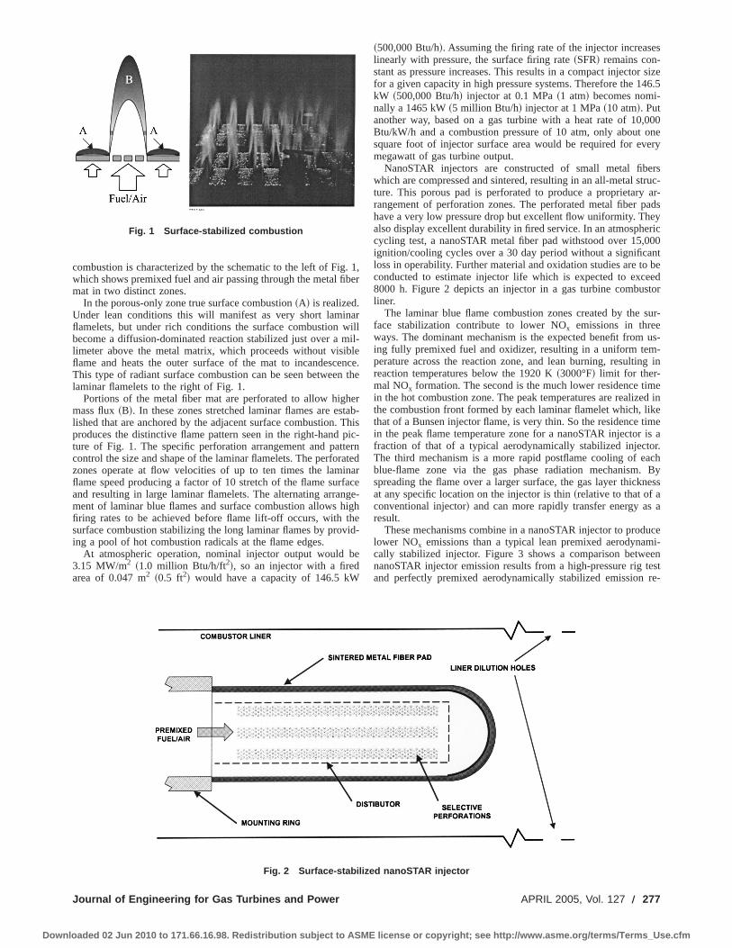
combustion is characterized by the schematic to the left of Fig. 1,which shows premixed fuel and air passing through the metal fibermat in two distinct zones.

In the porous-only zone true surface combustion~A! is realized.Under lean conditions this will manifest as very short laminarflamelets, but under rich conditions the surface combustion willbecome a diffusion-dominated reaction stabilized just over a mil-limeter above the metal matrix, which proceeds without visibleflame and heats the outer surface of the mat to incandescence.This type of radiant surface combustion can be seen between thelaminar flamelets to the right of Fig. 1.

Portions of the metal fiber mat are perforated to allow highermass flux~B!. In these zones stretched laminar flames are estab-lished that are anchored by the adjacent surface combustion. Thisproduces the distinctive flame pattern seen in the right-hand pic-ture of Fig. 1. The specific perforation arrangement and patterncontrol the size and shape of the laminar flamelets. The perforatedzones operate at flow velocities of up to ten times the laminarflame speed producing a factor of 10 stretch of the flame surfaceand resulting in large laminar flamelets. The alternating arrange-ment of laminar blue flames and surface combustion allows highfiring rates to be achieved before flame lift-off occurs, with thesurface combustion stabilizing the long laminar flames by provid-ing a pool of hot combustion radicals at the flame edges.

At atmospheric operation, nominal injector output would be3.15 MW/m2 ~1.0 million Btu/h/ft2!, so an injector with a firedarea of 0.047 m2 ~0.5 ft2! would have a capacity of 146.5 kW

~500,000 Btu/h!. Assuming the firing rate of the injector increaseslinearly with pressure, the surface firing rate~SFR! remains con-stant as pressure increases. This results in a compact injector sizefor a given capacity in high pressure systems. Therefore the 146.5kW ~500,000 Btu/h! injector at 0.1 MPa~1 atm! becomes nomi-nally a 1465 kW~5 million Btu/h! injector at 1 MPa~10 atm!. Putanother way, based on a gas turbine with a heat rate of 10,000Btu/kW/h and a combustion pressure of 10 atm, only about onesquare foot of injector surface area would be required for everymegawatt of gas turbine output.

NanoSTAR injectors are constructed of small metal fiberswhich are compressed and sintered, resulting in an all-metal struc-ture. This porous pad is perforated to produce a proprietary ar-rangement of perforation zones. The perforated metal fiber padshave a very low pressure drop but excellent flow uniformity. Theyalso display excellent durability in fired service. In an atmosphericcycling test, a nanoSTAR metal fiber pad withstood over 15,000ignition/cooling cycles over a 30 day period without a significantloss in operability. Further material and oxidation studies are to beconducted to estimate injector life which is expected to exceed8000 h. Figure 2 depicts an injector in a gas turbine combustorliner.

The laminar blue flame combustion zones created by the sur-face stabilization contribute to lower NOx emissions in threeways. The dominant mechanism is the expected benefit from us-ing fully premixed fuel and oxidizer, resulting in a uniform tem-perature across the reaction zone, and lean burning, resulting inreaction temperatures below the 1920 K~3000°F! limit for ther-mal NOx formation. The second is the much lower residence timein the hot combustion zone. The peak temperatures are realized inthe combustion front formed by each laminar flamelet which, likethat of a Bunsen injector flame, is very thin. So the residence timein the peak flame temperature zone for a nanoSTAR injector is afraction of that of a typical aerodynamically stabilized injector.The third mechanism is a more rapid postflame cooling of eachblue-flame zone via the gas phase radiation mechanism. Byspreading the flame over a larger surface, the gas layer thicknessat any specific location on the injector is thin~relative to that of aconventional injector! and can more rapidly transfer energy as aresult.

These mechanisms combine in a nanoSTAR injector to producelower NOx emissions than a typical lean premixed aerodynami-cally stabilized injector. Figure 3 shows a comparison betweennanoSTAR injector emission results from a high-pressure rig testand perfectly premixed aerodynamically stabilized emission re-

Fig. 1 Surface-stabilized combustion

Fig. 2 Surface-stabilized nanoSTAR injector



sults from a 1990 paper by Leonard and Correa@3#. In both casesthe tests were conducted at 1.01 MPa~10 atm! and 535–590 K~500–600°F! inlet temperatures.

In addition to lower emissions with a wide turndown window,nanoSTAR injectors can be designed to fit within existing com-bustor liners and fitted to existing fuel/air premixers without ex-tensive modification to the combustion equipment or pressurecase. Furthermore, they require no extraordinary control schemesor equipment beyond that which would be required for an aero-dynamically stabilized lean-premixed injector.

Past WorkA previous ASME paper~IJPGC2002-26088! described the de-

velopment of nanoSTAR from the proof-of-concept stage to pro-totype testing@4#. These tests were part of a development programpursued after a relationship was established between ALZETA andSolar Turbines. The initial target applications were Solar gas tur-bines in the 5–7 MW range.

Initial proof-of-concept tests occurred at the National EnergyTechnology Laboratory’s~NETL! Low Emission Combustion Testand Research facility in Morgantown, West Virginia. These high-pressure rig tests demonstrated operability and low emissions in asimulated gas turbine environment. The surface-stabilized injectorwas shown to operate stably over a pressure range of 0.18–1.24MPa ~1.8–12.2 atm! at the nominal values of flame temperatureand mass flow, so the operating envelope of the injector wasshown to be large. NOx emissions, at the lowest flame tempera-tures, were generally below 2 parts per million~corrected to 15%O2) and at times below 1 ppm. The highest value recorded wasless than 3.5 ppm.

After the success of the testing at NETL, additional proof-of-concept tests were conducted at Solar Turbines’ San Diego facili-ties. The most significant of these was a demonstration on anoperating gas turbine engine, which demonstrated the ability of a

nanoSTAR injector to provide stable operation through the startramp and across the engine load range. An existing modified 1MW Solar Saturn engine was used. The engine is outfitted with anexternal side-mounted combustor that allowed for easy hardwaremodification and instrumentation. The side-mounted design alsoprovides variable geometry in the form of butterfly valves to con-trol the air flow split between the primary and dilution zones.

On the first day of testing, the surface-stabilized injector tookthe engine through the start ramp to the point of starter drop-out,the idle point where combustion provides enough energy to main-tain air flow through the engine. By the second day of testingstable operation up to 92% engine speed was achieved. Figure 4shows the gas producer speed and NOx emissions from this testrun. No effort was made to optimize emissions performance asoperational characteristics of the technology were the focus of thedemonstration. However, NOx emissions were well below thetypical dry low NOx value of 25 ppm~15% O2). On the third andfinal day of testing the start ramp was completely automated. Theengine was brought to idle speed entirely by the control systemexcept for manual adjustment of the air flow split. As controlalgorithms were developed, several system shutdowns occurred,and the nanoSTAR injector responded with reliable ignition andperformance through several start ramps. The engine was operatedto 95% speed before a high temperature limit upstream of theturbine section~unrelated to the surface-stabilized injector! pre-vented further increase.

The proof-of-concept tests confirmed that nanoSTAR technol-ogy can operate under the conditions of pressure and temperaturefound in a gas turbine engine, and can in fact provide the motivepower for an actual engine. The next phase was to design, test,and demonstrate a prototype injector for Solar’s Taurus 60 engine.

First, the technology itself was refined based on the results ofthe previous tests. A new generation of monolithic nanoSTARinjectors were produced. This produced a simplified combustionsurface free of welds or other joints, and allowed the injectors to

Fig. 3 Surface-stabilized compared to aerodynamically stabilized emission results; both testsconducted at 1.01 MPa „10 atm … pressure and 535–590 K „500–600°F… inlet temperatures



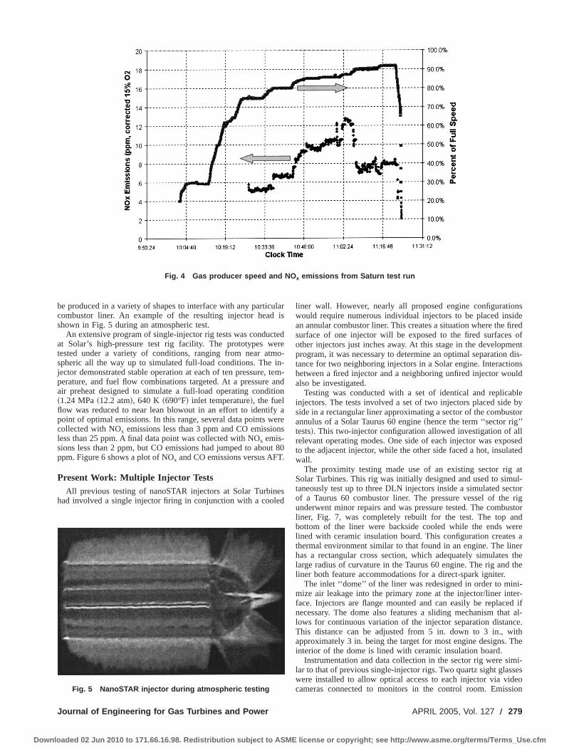
be produced in a variety of shapes to interface with any particularcombustor liner. An example of the resulting injector head isshown in Fig. 5 during an atmospheric test.

An extensive program of single-injector rig tests was conductedat Solar’s high-pressure test rig facility. The prototypes weretested under a variety of conditions, ranging from near atmo-spheric all the way up to simulated full-load conditions. The in-jector demonstrated stable operation at each of ten pressure, tem-perature, and fuel flow combinations targeted. At a pressure andair preheat designed to simulate a full-load operating condition~1.24 MPa~12.2 atm!, 640 K ~690°F! inlet temperature!, the fuelflow was reduced to near lean blowout in an effort to identify apoint of optimal emissions. In this range, several data points werecollected with NOx emissions less than 3 ppm and CO emissionsless than 25 ppm. A final data point was collected with NOx emis-sions less than 2 ppm, but CO emissions had jumped to about 80ppm. Figure 6 shows a plot of NOx and CO emissions versus AFT.

Present Work: Multiple Injector TestsAll previous testing of nanoSTAR injectors at Solar Turbines

had involved a single injector firing in conjunction with a cooled

liner wall. However, nearly all proposed engine configurationswould require numerous individual injectors to be placed insidean annular combustor liner. This creates a situation where the firedsurface of one injector will be exposed to the fired surfaces ofother injectors just inches away. At this stage in the developmentprogram, it was necessary to determine an optimal separation dis-tance for two neighboring injectors in a Solar engine. Interactionsbetween a fired injector and a neighboring unfired injector wouldalso be investigated.

Testing was conducted with a set of identical and replicableinjectors. The tests involved a set of two injectors placed side byside in a rectangular liner approximating a sector of the combustorannulus of a Solar Taurus 60 engine~hence the term ‘‘sector rig’’tests!. This two-injector configuration allowed investigation of allrelevant operating modes. One side of each injector was exposedto the adjacent injector, while the other side faced a hot, insulatedwall.

The proximity testing made use of an existing sector rig atSolar Turbines. This rig was initially designed and used to simul-taneously test up to three DLN injectors inside a simulated sectorof a Taurus 60 combustor liner. The pressure vessel of the rigunderwent minor repairs and was pressure tested. The combustorliner, Fig. 7, was completely rebuilt for the test. The top andbottom of the liner were backside cooled while the ends werelined with ceramic insulation board. This configuration creates athermal environment similar to that found in an engine. The linerhas a rectangular cross section, which adequately simulates thelarge radius of curvature in the Taurus 60 engine. The rig and theliner both feature accommodations for a direct-spark igniter.

The inlet ‘‘dome’’ of the liner was redesigned in order to mini-mize air leakage into the primary zone at the injector/liner inter-face. Injectors are flange mounted and can easily be replaced ifnecessary. The dome also features a sliding mechanism that al-lows for continuous variation of the injector separation distance.This distance can be adjusted from 5 in. down to 3 in., withapproximately 3 in. being the target for most engine designs. Theinterior of the dome is lined with ceramic insulation board.

Instrumentation and data collection in the sector rig were simi-lar to that of previous single-injector rigs. Two quartz sight glasseswere installed to allow optical access to each injector via videocameras connected to monitors in the control room. Emission

Fig. 4 Gas producer speed and NO x emissions from Saturn test run

Fig. 5 NanoSTAR injector during atmospheric testing



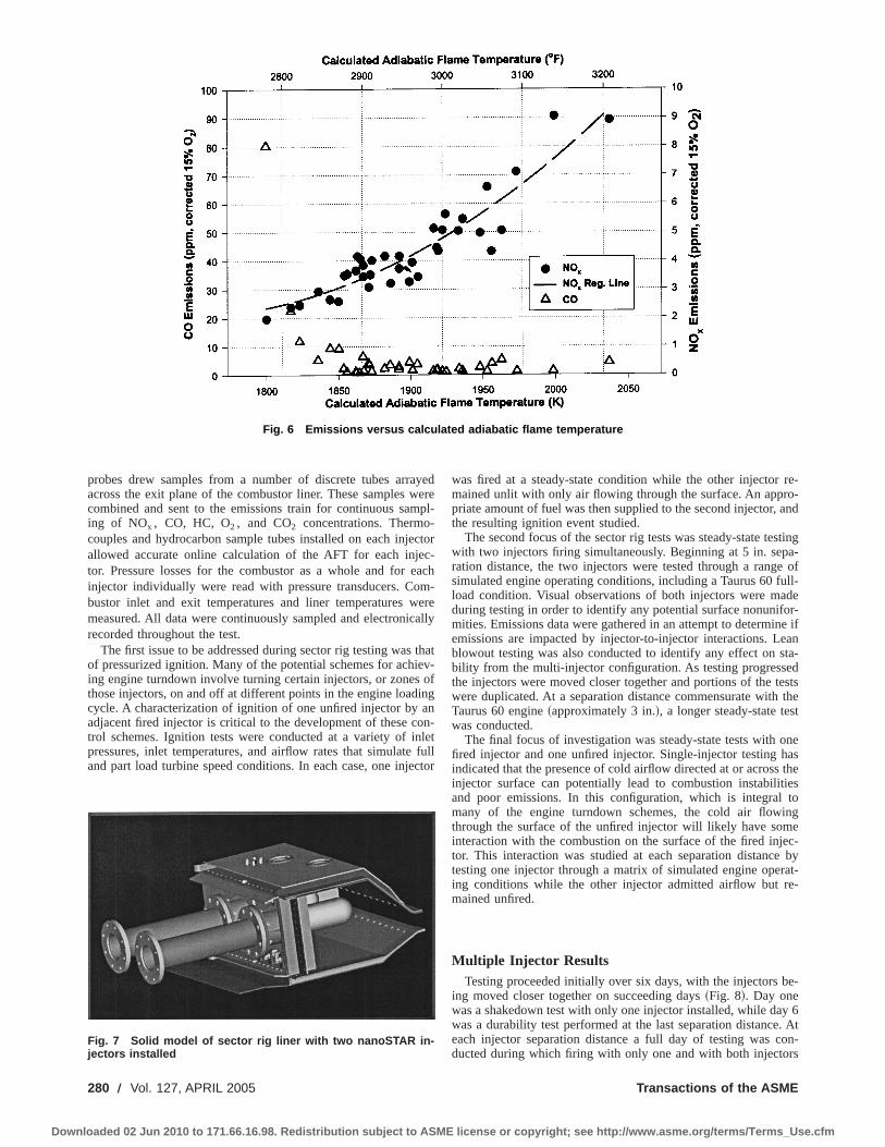
probes drew samples from a number of discrete tubes arrayedacross the exit plane of the combustor liner. These samples werecombined and sent to the emissions train for continuous sampl-ing of NOx , CO, HC, O2 , and CO2 concentrations. Thermo-couples and hydrocarbon sample tubes installed on each injectorallowed accurate online calculation of the AFT for each injec-tor. Pressure losses for the combustor as a whole and for eachinjector individually were read with pressure transducers. Com-bustor inlet and exit temperatures and liner temperatures weremeasured. All data were continuously sampled and electronicallyrecorded throughout the test.

The first issue to be addressed during sector rig testing was thatof pressurized ignition. Many of the potential schemes for achiev-ing engine turndown involve turning certain injectors, or zones ofthose injectors, on and off at different points in the engine loadingcycle. A characterization of ignition of one unfired injector by anadjacent fired injector is critical to the development of these con-trol schemes. Ignition tests were conducted at a variety of inletpressures, inlet temperatures, and airflow rates that simulate fulland part load turbine speed conditions. In each case, one injector

was fired at a steady-state condition while the other injector re-mained unlit with only air flowing through the surface. An appro-priate amount of fuel was then supplied to the second injector, andthe resulting ignition event studied.

The second focus of the sector rig tests was steady-state testingwith two injectors firing simultaneously. Beginning at 5 in. sepa-ration distance, the two injectors were tested through a range ofsimulated engine operating conditions, including a Taurus 60 full-load condition. Visual observations of both injectors were madeduring testing in order to identify any potential surface nonunifor-mities. Emissions data were gathered in an attempt to determine ifemissions are impacted by injector-to-injector interactions. Leanblowout testing was also conducted to identify any effect on sta-bility from the multi-injector configuration. As testing progressedthe injectors were moved closer together and portions of the testswere duplicated. At a separation distance commensurate with theTaurus 60 engine~approximately 3 in.!, a longer steady-state testwas conducted.

The final focus of investigation was steady-state tests with onefired injector and one unfired injector. Single-injector testing hasindicated that the presence of cold airflow directed at or across theinjector surface can potentially lead to combustion instabilitiesand poor emissions. In this configuration, which is integral tomany of the engine turndown schemes, the cold air flowingthrough the surface of the unfired injector will likely have someinteraction with the combustion on the surface of the fired injec-tor. This interaction was studied at each separation distance bytesting one injector through a matrix of simulated engine operat-ing conditions while the other injector admitted airflow but re-mained unfired.

Multiple Injector ResultsTesting proceeded initially over six days, with the injectors be-

ing moved closer together on succeeding days~Fig. 8!. Day onewas a shakedown test with only one injector installed, while day 6was a durability test performed at the last separation distance. Ateach injector separation distance a full day of testing was con-ducted during which firing with only one and with both injectors

Fig. 6 Emissions versus calculated adiabatic flame temperature

Fig. 7 Solid model of sector rig liner with two nanoSTAR in-jectors installed



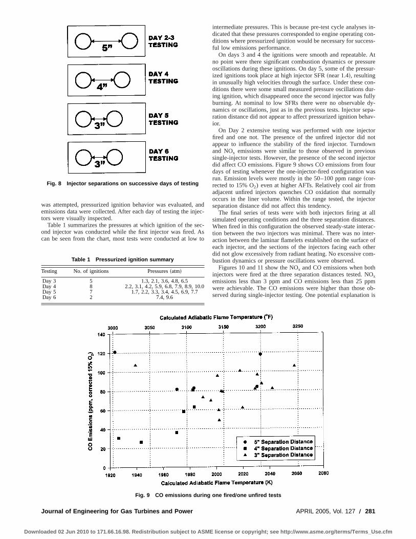
was attempted, pressurized ignition behavior was evaluated, andemissions data were collected. After each day of testing the injec-tors were visually inspected.

Table 1 summarizes the pressures at which ignition of the sec-ond injector was conducted while the first injector was fired. Ascan be seen from the chart, most tests were conducted at low to

intermediate pressures. This is because pre-test cycle analyses in-dicated that these pressures corresponded to engine operating con-ditions where pressurized ignition would be necessary for success-ful low emissions performance.

On days 3 and 4 the ignitions were smooth and repeatable. Atno point were there significant combustion dynamics or pressureoscillations during these ignitions. On day 5, some of the pressur-ized ignitions took place at high injector SFR~near 1.4!, resultingin unusually high velocities through the surface. Under these con-ditions there were some small measured pressure oscillations dur-ing ignition, which disappeared once the second injector was fullyburning. At nominal to low SFRs there were no observable dy-namics or oscillations, just as in the previous tests. Injector sepa-ration distance did not appear to affect pressurized ignition behav-ior.

On Day 2 extensive testing was performed with one injectorfired and one not. The presence of the unfired injector did notappear to influence the stability of the fired injector. Turndownand NOx emissions were similar to those observed in previoussingle-injector tests. However, the presence of the second injectordid affect CO emissions. Figure 9 shows CO emissions from fourdays of testing whenever the one-injector-fired configuration wasrun. Emission levels were mostly in the 50–100 ppm range~cor-rected to 15% O2) even at higher AFTs. Relatively cool air fromadjacent unfired injectors quenches CO oxidation that normallyoccurs in the liner volume. Within the range tested, the injectorseparation distance did not affect this tendency.

The final series of tests were with both injectors firing at allsimulated operating conditions and the three separation distances.When fired in this configuration the observed steady-state interac-tion between the two injectors was minimal. There was no inter-action between the laminar flamelets established on the surface ofeach injector, and the sections of the injectors facing each otherdid not glow excessively from radiant heating. No excessive com-bustion dynamics or pressure oscillations were observed.

Figures 10 and 11 show the NOx and CO emissions when bothinjectors were fired at the three separation distances tested. NOxemissions less than 3 ppm and CO emissions less than 25 ppmwere achievable. The CO emissions were higher than those ob-served during single-injector testing. One potential explanation is

Fig. 8 Injector separations on successive days of testing

Fig. 9 CO emissions during one fired Õone unfired tests

Table 1 Pressurized ignition summary

Testing No. of ignitions Pressures~atm!

Day 3 5 1.3, 2.1, 3.6, 4.8, 6.5Day 4 8 2.2, 3.1, 4.2, 5.9, 6.8, 7.9, 8.9, 10.0Day 5 7 1.7, 2.2, 3.3, 3.4, 4.5, 6.9, 7.7Day 6 2 7.4, 9.6



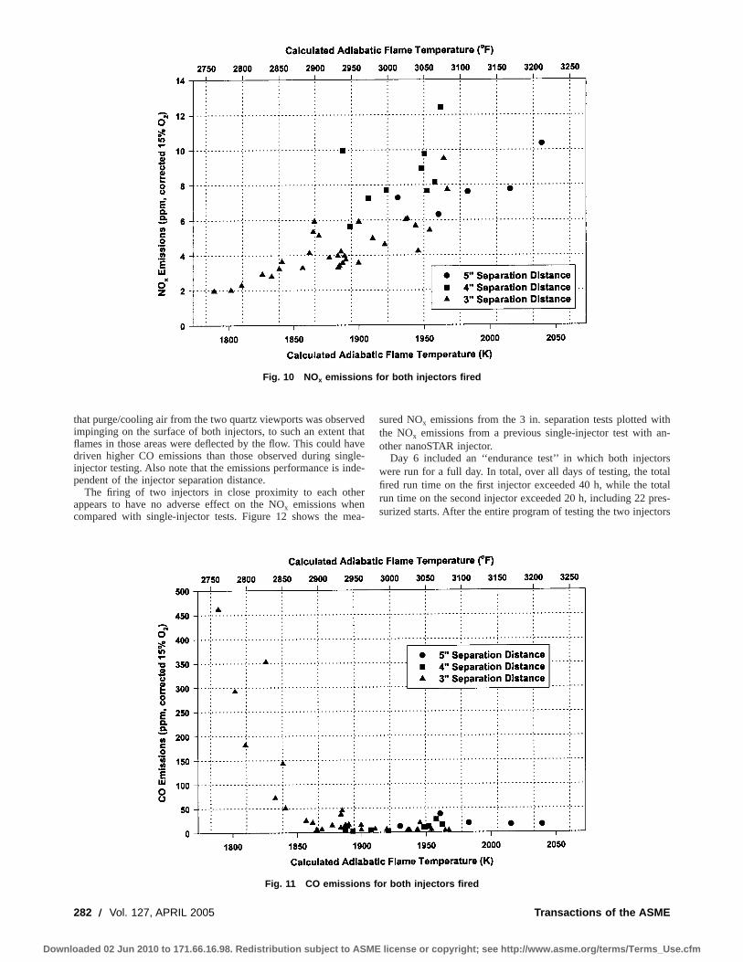
that purge/cooling air from the two quartz viewports was observedimpinging on the surface of both injectors, to such an extent thatflames in those areas were deflected by the flow. This could havedriven higher CO emissions than those observed during single-injector testing. Also note that the emissions performance is inde-pendent of the injector separation distance.

The firing of two injectors in close proximity to each otherappears to have no adverse effect on the NOx emissions whencompared with single-injector tests. Figure 12 shows the mea-

sured NOx emissions from the 3 in. separation tests plotted withthe NOx emissions from a previous single-injector test with an-other nanoSTAR injector.

Day 6 included an ‘‘endurance test’’ in which both injectorswere run for a full day. In total, over all days of testing, the totalfired run time on the first injector exceeded 40 h, while the totalrun time on the second injector exceeded 20 h, including 22 pres-surized starts. After the entire program of testing the two injectors

Fig. 10 NOx emissions for both injectors fired

Fig. 11 CO emissions for both injectors fired



were examined and neither showed any signs of excessive agingdue to the proximity testing. Figure 13 shows before and afterpictures of the first injector.

Higher Pressure OperationPrevious tests at multiple facilities clearly established the vi-

ability of nanoSTAR surface-stabilized combustion technology atpressures and volumetric heat release rates consistent with indus-trial gas turbines with pressure ratios up to 12. Higher inlet tem-peratures and pressure ratios are required to increase engine effi-ciency and are encountered in higher output engines such as Solar

Turbines’ 13.5 MW Titan 130. This engine operates at a pressureratio of 16 as opposed to 12 for the Taurus 60. To assess thefeasibility of applying the technology to higher pressure ratio en-gines, a prototype Taurus 60 nanoSTAR injector was rig testedunder simulated Titan 130 pressure and temperature conditions.

As in previous tests the injector was ignited at near-atmosphericconditions and ramped through a series of pressure/temperaturecombinations, however, this time the ramp was continued beyondTaurus 60 full load conditions, ultimately reaching 1.68 MPa~16.6 atm! and 670 K~750°F!. At these elevated pressure and inlettemperature conditions, the injector displayed greatly enhanced

Fig. 12 Comparison of day 6 NO x data with data from a single injector test on Dec. 7, 2001

Fig. 13 Pictures of the first sector rig injector before testing „left … and aftertesting



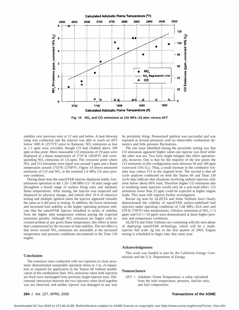
stability over previous tests at 12 atm and below. A lean blowoutramp was conducted and the injector was able to reach an AFTbelow 1685 K~2575°F! prior to flameout. NOx emissions as lowas 1.1 ppm were recorded, though CO had climbed above 100ppm at that point. More reasonable CO emissions of 29 ppm weredisplayed at a flame temperature of 1710 K~2618°F! and corre-sponding NOx emissions of 1.6 ppm. The crossover point whereNOx and CO emissions were equal was around 3 ppm and a flametemperature around 1755°K~2700°F!. Figure 14 shows measuredemissions of CO and NOx at the nominal 1.6 MPa~16 atm! pres-sure condition.

During these tests the nanoSTAR injector displayed stable, low-emissions operation in the 1.20–1.68 MPa~12–16 atm! range andthroughout a broad range of surface firing rates and adiabaticflame temperatures. After testing, the injector was inspected anddisplayed no physical change, and indeed after 10 h of intensivetesting and multiple ignition starts the injector appeared virtuallythe same as it did prior to testing. In addition, the lower emissionsand increased lean stability at the higher operating pressure indi-cate that the nanoSTAR injector benefited in terms of stabilityfrom the higher inlet temperature without paying the expectedemissions penalty. Although NOx emissions are higher with in-creased preheat at any given flame temperature, this effect is morethan counteracted by the increase in lean stability. The net effect isthat lower overall NOx emissions are attainable at the increasedtemperature and pressure conditions encountered in the Titan 130engine.

ConclusionThe extensive tests conducted with two injectors in close prox-

imity demonstrated sustainable operation down to 3 in. of separa-tion as required for application in the Taurus 60 without modifi-cation of the combustion liner. NOx emissions when both injectorsare fired were unchanged from previous single-injector tests. Det-rimental interaction between the two injectors when fired togetherwas not observed, and neither injector was damaged in any way

by proximity firing. Pressurized ignition was successful and wasrepeated at several pressures with no observable combustion dy-namics and little pressure fluctuations.

The one issue identified during the proximity testing was thatCO emissions appeared higher when one injector was fired whilethe other was not. Two facts might mitigate this effect operation-ally, however. One is that for the majority of the test points theCO emissions in this configuration were between 50 and 100 ppm~corrected 15% O2). Thus, a small increase in the combustor vol-ume may reduce CO to the targeted level. The second is that allcycle analyses conducted on both the Taurus 60 and Titan 130cycle data indicate that situations involving unfired injectors onlyarise below about 60% load. Therefore higher CO emissions dueto nonfiring some injectors would only be a part-load effect. COemissions lower than 25 ppm could be expected at higher engineloads. This issue still requires further investigation.

Recent rig tests by ALZETA and Solar Turbines have clearlydemonstrated the viability of nanoSTAR surface-stabilized fuelinjectors under operating conditions of 1.68 MPa~16.6 atm! and670 K ~750°F! inlet temperatures. Ultralow emissions of NOx ~,3ppm! and CO~,10 ppm! were demonstrated at these higher pres-sure and temperature conditions.

ALZETA and Solar Turbines are continuing with the next phaseof deploying nanoSTAR technology, which will be a multi-injector full scale rig test in the first quarter of 2003. Enginetesting is scheduled to begin later that same year.

AcknowledgmentsThis work was funded in part by the California Energy Com-

mission and the U.S. Department of Energy.

Nomenclature

AFT 5 Adiabatic Flame Temperature; a value calculatedfrom the inlet temperature, pressure, fuel/air ratio,and fuel composition.

Fig. 14 NOx and CO emissions at 116 MPa „16 atm … versus AFT



SFR 5 Surface Firing Rate; injector firing rate per squarefoot of injector fired surface area per atmosphere ofpressure. Closely tied to injector pressure drop andfiring rate.

References@1# Vandervort, C. L., 2001, ‘‘9 ppm NOx /CO Combustion System for ‘‘F’’ Class

Industrial Gas Turbines,’’ ASME J. Eng. Gas Turbines Power,123, pp. 317–321.

@2# Yee, D. K., Lundberg, K., and Weakley, C. K., 2001, ‘‘Field Demonstration of

a 1.5 MW Industrial Gas Turbine With a Low Emissions Catalytica Combus-tion System,’’ ASME J. Eng. Gas Turbines Power,123, pp. 550–556.

@3# Leonard, G. L., and Correa, S. M., 1990, ‘‘NOx Formation in Premixed High-Pressure Lean Methane Flames,’’ Fossil Fuel Combustion Symposium 1990, S.N. Singh, ed., American Society of Mechanical Engineers, New York, pp.69–74.

@4# Weakley, C. K., Greenberg, S. J., Kendall, R. M., McDougald, N. K., andArellano, L. O., 2002, ‘‘Development of Surface-Stabilized Fuel InjectorsWith Sub-Three ppm NOx Emissions,’’ ASME Paper No. IJPGC2002-26088,presented at the 2002 International Joint Power Generation Conference, Phoe-nix, AZ, 24–26 June, 2002.



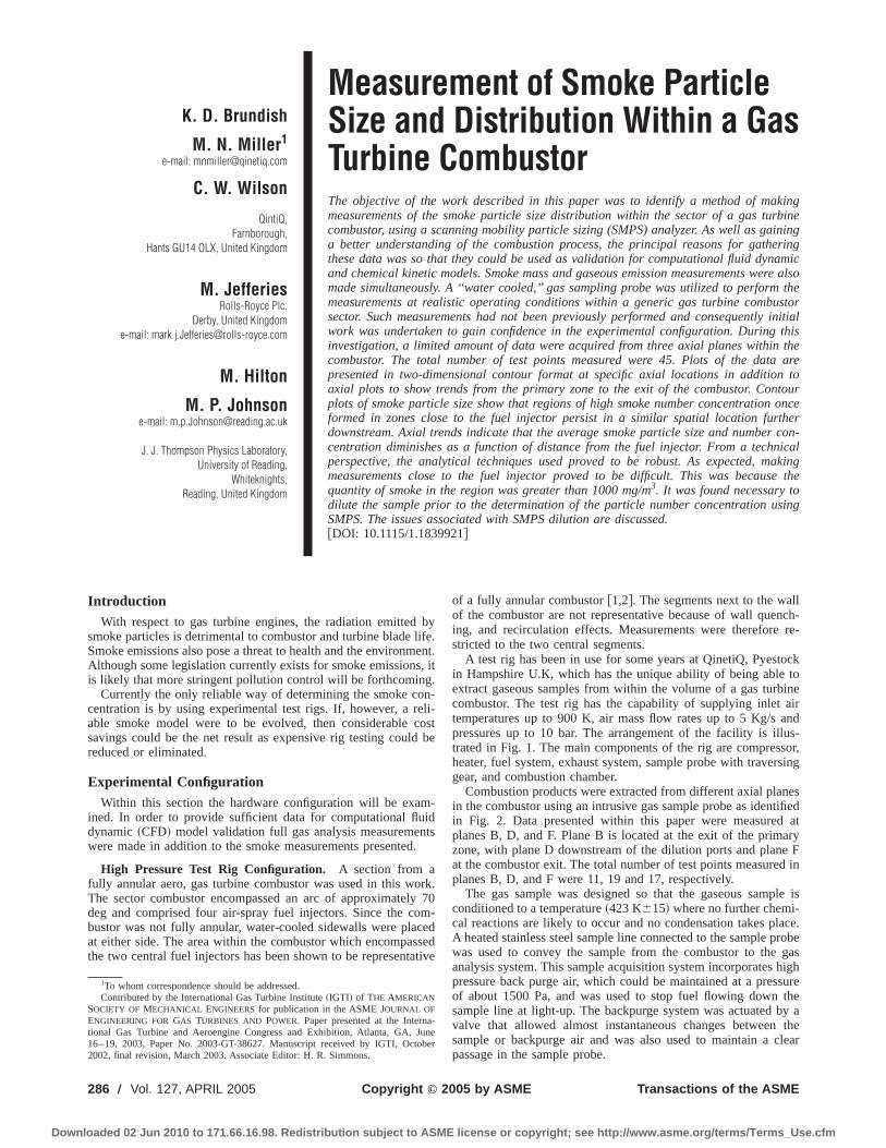
K. D. Brundish

M. N. Miller1


C. W. Wilson

QintiQ,Farnborough,

Hants GU14 OLX, United Kingdom

M. JefferiesRolls-Royce Plc,

Derby, United Kingdome-mail: [email protected]

M. Hilton

M. P. Johnsone-mail: [email protected]

J. J. Thompson Physics Laboratory,University of Reading,

Whiteknights,Reading, United Kingdom

Measurement of Smoke ParticleSize and Distribution Within a GasTurbine CombustorThe objective of the work described in this paper was to identify a method of makingmeasurements of the smoke particle size distribution within the sector of a gas turbinecombustor, using a scanning mobility particle sizing (SMPS) analyzer. As well as gaininga better understanding of the combustion process, the principal reasons for gatheringthese data was so that they could be used as validation for computational fluid dynamicand chemical kinetic models. Smoke mass and gaseous emission measurements were alsomade simultaneously. A ‘‘water cooled,’’ gas sampling probe was utilized to perform themeasurements at realistic operating conditions within a generic gas turbine combustorsector. Such measurements had not been previously performed and consequently initialwork was undertaken to gain confidence in the experimental configuration. During thisinvestigation, a limited amount of data were acquired from three axial planes within thecombustor. The total number of test points measured were 45. Plots of the data arepresented in two-dimensional contour format at specific axial locations in addition toaxial plots to show trends from the primary zone to the exit of the combustor. Contourplots of smoke particle size show that regions of high smoke number concentration onceformed in zones close to the fuel injector persist in a similar spatial location furtherdownstream. Axial trends indicate that the average smoke particle size and number con-centration diminishes as a function of distance from the fuel injector. From a technicalperspective, the analytical techniques used proved to be robust. As expected, makingmeasurements close to the fuel injector proved to be difficult. This was because thequantity of smoke in the region was greater than 1000 mg/m3. It was found necessary todilute the sample prior to the determination of the particle number concentration usingSMPS. The issues associated with SMPS dilution are discussed.@DOI: 10.1115/1.1839921#

IntroductionWith respect to gas turbine engines, the radiation emitted by

smoke particles is detrimental to combustor and turbine blade life.Smoke emissions also pose a threat to health and the environment.Although some legislation currently exists for smoke emissions, itis likely that more stringent pollution control will be forthcoming.

Currently the only reliable way of determining the smoke con-centration is by using experimental test rigs. If, however, a reli-able smoke model were to be evolved, then considerable costsavings could be the net result as expensive rig testing could bereduced or eliminated.

Experimental ConfigurationWithin this section the hardware configuration will be exam-

ined. In order to provide sufficient data for computational fluiddynamic~CFD! model validation full gas analysis measurementswere made in addition to the smoke measurements presented.

High Pressure Test Rig Configuration. A section from afully annular aero, gas turbine combustor was used in this work.The sector combustor encompassed an arc of approximately 70deg and comprised four air-spray fuel injectors. Since the com-bustor was not fully annular, water-cooled sidewalls were placedat either side. The area within the combustor which encompassedthe two central fuel injectors has been shown to be representative

of a fully annular combustor@1,2#. The segments next to the wallof the combustor are not representative because of wall quench-ing, and recirculation effects. Measurements were therefore re-stricted to the two central segments.

A test rig has been in use for some years at QinetiQ, Pyestockin Hampshire U.K, which has the unique ability of being able toextract gaseous samples from within the volume of a gas turbinecombustor. The test rig has the capability of supplying inlet airtemperatures up to 900 K, air mass flow rates up to 5 Kg/s andpressures up to 10 bar. The arrangement of the facility is illus-trated in Fig. 1. The main components of the rig are compressor,heater, fuel system, exhaust system, sample probe with traversinggear, and combustion chamber.

Combustion products were extracted from different axial planesin the combustor using an intrusive gas sample probe as identifiedin Fig. 2. Data presented within this paper were measured atplanes B, D, and F. Plane B is located at the exit of the primaryzone, with plane D downstream of the dilution ports and plane Fat the combustor exit. The total number of test points measured inplanes B, D, and F were 11, 19 and 17, respectively.

The gas sample was designed so that the gaseous sample isconditioned to a temperature~423 K615! where no further chemi-cal reactions are likely to occur and no condensation takes place.A heated stainless steel sample line connected to the sample probewas used to convey the sample from the combustor to the gasanalysis system. This sample acquisition system incorporates highpressure back purge air, which could be maintained at a pressureof about 1500 Pa, and was used to stop fuel flowing down thesample line at light-up. The backpurge system was actuated by avalve that allowed almost instantaneous changes between thesample or backpurge air and was also used to maintain a clearpassage in the sample probe.

1To whom correspondence should be addressed.Contributed by the International Gas Turbine Institute~IGTI! of THE AMERICAN




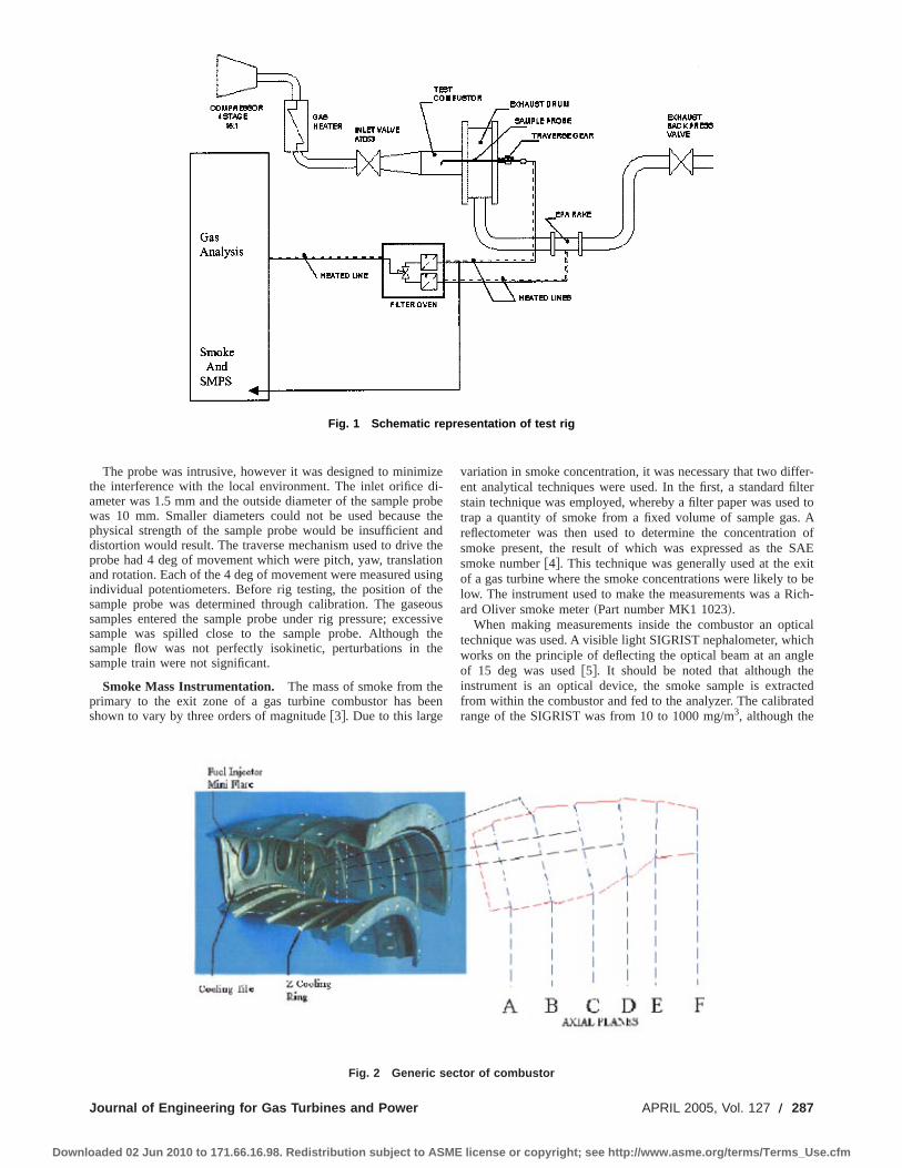
The probe was intrusive, however it was designed to minimizethe interference with the local environment. The inlet orifice di-ameter was 1.5 mm and the outside diameter of the sample probewas 10 mm. Smaller diameters could not be used because thephysical strength of the sample probe would be insufficient anddistortion would result. The traverse mechanism used to drive theprobe had 4 deg of movement which were pitch, yaw, translationand rotation. Each of the 4 deg of movement were measured usingindividual potentiometers. Before rig testing, the position of thesample probe was determined through calibration. The gaseoussamples entered the sample probe under rig pressure; excessivesample was spilled close to the sample probe. Although thesample flow was not perfectly isokinetic, perturbations in thesample train were not significant.

Smoke Mass Instrumentation. The mass of smoke from theprimary to the exit zone of a gas turbine combustor has beenshown to vary by three orders of magnitude@3#. Due to this large

variation in smoke concentration, it was necessary that two differ-ent analytical techniques were used. In the first, a standard filterstain technique was employed, whereby a filter paper was used totrap a quantity of smoke from a fixed volume of sample gas. Areflectometer was then used to determine the concentration ofsmoke present, the result of which was expressed as the SAEsmoke number@4#. This technique was generally used at the exitof a gas turbine where the smoke concentrations were likely to below. The instrument used to make the measurements was a Rich-ard Oliver smoke meter~Part number MK1 1023!.

When making measurements inside the combustor an opticaltechnique was used. A visible light SIGRIST nephalometer, whichworks on the principle of deflecting the optical beam at an angleof 15 deg was used@5#. It should be noted that although theinstrument is an optical device, the smoke sample is extractedfrom within the combustor and fed to the analyzer. The calibratedrange of the SIGRIST was from 10 to 1000 mg/m3, although the

Fig. 1 Schematic representation of test rig

Fig. 2 Generic sector of combustor



analyzer read up to 2000 mg/m3. The SIGRIST was initially cali-brated against a known mass of smoke generated by a combustor@6#. Subsequent checks on the optics were undertaken using re-flective rods. Maximum errors associated with the optical tech-nique have been found to be625%.

SMPS Instrumentation. In order to determine the numberconcentration and size distribution of the smoke particulates, aTSI, scanning mobility particle sizing~SMPS! analyzer was used.The SMPS system measures the size distribution of aerosols in thesize range from 14 to about 800 nm using an electrical mobilitydetection technique. The SMPS analyzer was connected to thesame dedicated smoke sample line which also incorporated theSIGRIST and the SAE measuring instruments. A direct compari-son between the different analytical techniques could then bemade. It was important when using the SMPS analyzer that thesample was fed at a constant pressure. This was achieved by re-ducing the sample pressure to near atmospheric. This reduction inpressure must be achieved with minimal disruption to the flow inorder to reduce effects on smoke measurements and was achievedusing the configuration identified in Fig. 3.

The sample is expanded slowly into a large volume that isvented to atmosphere downstream. A small percentage of thesample flows into the SMPS instrument through a secondarysample tube located in the center of the large volume. This ensuresthat the pressure is reduced while maintaining sample fidelity.

The SMPS system measures the size distribution of particulatesusing an electrical mobility technique. A radioactive Kr-85 sourceis used to neutralize and charge incoming particulates. Thecharged particles then enter a classifier where they are sequen-tially separated by electrostatic repulsion.

After the sample has been ‘‘classified’’ by the SMPS, thesample was drawn, by a pump, through a condensation particlecounter~CPC! to determine number concentration.

Sample Dilution. In order to make SMPS measurementswithin the combustor; it was necessary to dilute the gaseoussample before determination of the particle size and distribution.There are several reasons why the sample must be diluted prior tomeasurement. The main ones are related to water of combustionconcentration, particulate number concentration, and coagulationof smoke particulates in the sample line.

Particulate number concentration is a concern when values ex-ceed 1E7 particles/cm3 for any given size range. This instrumentis not able to measure such high values and defaults to a statisticalapproach~photometric effect!. Dilution reduces the likelihood ofthis occurring as the particle number counts are reduced.

Water of combustion only becomes a problem if the dewpointof the gaseous water is exceeded and particulates are lost in thecondensate. Heating the sample lines to 423 K ensures no conden-sation takes place in the sample line. It was not, however, possibleto heat the lines within the SMPS analyzer, therefore the dewpoint has to be adjusted by dilution so that none of the particulatesare lost due to condensation.

Coagulation of smoke particulates occurs when the individualparticles collide and stick to each other@7#. Upon initial coagula-tion, more and more of the particulates collide, thus forming ever-larger particulates. When initially formed, smoke particulates arevery small, these particulates upon coagulating diminish in num-ber but increase in size. The effect of coagulation is shown in Fig.4 which shows smoke particulates magnified 310,000 times. It canbe seen that when they coagulate they become larger and losetheir spherical shape. This image, although collected from an aeroengine, was not acquired from the combustor used in this work.Diluting the sample reduces the proximity of the particulates toeach other thus increasing the mean free path before collision andpossible coagulation occurs.

The dilution air was generated using a compressor and thenfiltered by using a two stage BOLSTEN filtering system. Thissystem removes particles down to a size of 0.01mm, as well aswater and oil. The total particulate number concentration for thisfiltered air was measured using the SMPS and found to be be-tween 20 and 50 particles/cm3. The need for filtering the dilutionair was shown by checking ambient air concentration values in thetest control room which were found to be between 3000–8000particles/cm3. The dilution air line was heated to 42365 K for alength of about 1 m prior to joining a Y piece. The Y piece al-lowed the dilution air to merge with the gas sample as depicted inFig. 5. The reason that the air was heated was to offset any po-tential effects upon the sample.

The gas analysis system was used to determine the dilutionratio of the sample. The gas analysis facility consisted of a suite ofgas analyzers, which were used to determine the concentration ofpollutants. The analysers that were available are shown in Table 1.

It can be seen from Table 1 that the CO and CO2 analyzers

Fig. 3 Pressure regulation system

Fig. 4 Smoke particulates magnified 310,000 times



covered a number of ranges to enhance the accuracy of the mea-surements. With the cycles considered, the CO2 concentration be-tween the combustor face and the exit of the combustor couldvary between 0.5% and 15%, hence the need for two analyzers.The gas analysis system used conforms to the requirements of theInternational Civil Aviation Organization, July 1993@8#.

Dilution was determined by taking a gas analysis measurementbefore and after the dilution air was added to the sample. NO,NOX , O2 , CO2 , total hydrocarbons and CO were measured ateach of the test points. The most stable chemical species, how-ever, was CO2 , and this was used to determine the dilution ratio.Two individual CO2 analyzers were used to measure the concen-tration of the specific species, and the ranges of the two analyzerswere 0%–2% and 0%–15%.

The dilution ratio as determined by CO2 was checked againstvalues obtained using NOX (NO21NO) and the results obtainedwere in good agreement. Although NOX could be used to deter-mine the dilution ratio, NO and NO2 measured individually couldnot. This is because of possible chemical reactions occurring inthe sample line prior to the measurement of the species. The maxi-mum uncertainty associated with the dilution ratio was611% atdilution ratios up to 35, while at a dilution ratio of 150 the uncer-tainty was623%.

Line Losses. Work undertaken by Hurley@9# has shown thatsmoke particulates are lost on the walls of the sample line as theyare transported to the smoke measuring equipment. Hurley de-rived the following line loss equation~E1!. The equation takesinto account factors such as velocity, composition of sample line,line diameter, and length:

n/n05exp~2~1.05E24V12.27E24!L/DV!, (E1)

where n/n05The ratio of smoke particles coming out of thesample line~n! to those entering the line.

V5velocity ~m/s!L5sample line length~m!D5sample line internal diameter~m!The calculated line loss found for the operating conditions used

in this work was found to be between 21% and 24%. All datapresented in this paper have been corrected for line loss.

Summary of Experimental Configuration. A number offactors affect the accuracy of the SMPS measurements, some ofwhich are reduced through the use of dilution and conditionedsample lines. The experiment has been configured to minimize allof the associated errors, although it is not possible to determine anoverall systematic error, the smoke measurements performed willbe compared to more traditional techniques to gain confidence inthe data. Although it is desirable to maximize the dilution ratio,the sensitivity of the gas analysis measurement system presented apractical limitation. SMPS measurements had not been previouslyperformed within the combustor and as a consequence the mini-mum required dilution was unknown at the commencement of thetesting and had to be derived experimentally.

Determination of Minimum Dilution Ratio

Dilution Effects With Respect to Probe Location. Smokeand gas analysis measurements were made at a number of axialplanes within the combustor: B, D, and F as illustrated in Fig. 2.Preliminary tests were undertaken to ascertain the effect of dilu-tion upon the particulate number concentration in each of the axialplanes.

Figure 6 shows a plot of normalized particulate number con-centration versus particulate size for an individual test point takenwithin plane F. The diluted data have been multiplied by the di-lution factor as determined from the gas analysis measurements.The dilution value as determined from the CO2 measurements wasfound to be 19. The mean particle size for the diluted sample wasfound to be 50 nm while for the undiluted test point the value was52 nm. The fact that the mean particle size does not significantlychange suggests that coagulation is not a problem in this axialplane.

Figure 7 shows a diluted test point multiplied by the dilutionfactor, and also the undiluted test point acquired at the same spa-tial location in plane D. Gas analysis measurements at this testpoint suggest that the dilution ratio was 19. The value for themean particle size of diluted sample was found to be 67 nm while

Fig. 5 Layout of the dilution system

Table 1 Analysers used

Type of analyzer TechniqueRange

%

Carbon dioxide Infrared 0–15Carbon dioxide Infrared 0–2Carbon monoxide Infrared 0–0.05Carbon monoxide Infrared 0–1Carbon monoxide Infrared 0–15Total HC Flame ionization 0–10Hydrogen Chromatography 0–10Oxygen Paramagnetic 0–30Nitrogen oxides Chemiluminescense 0–0.1



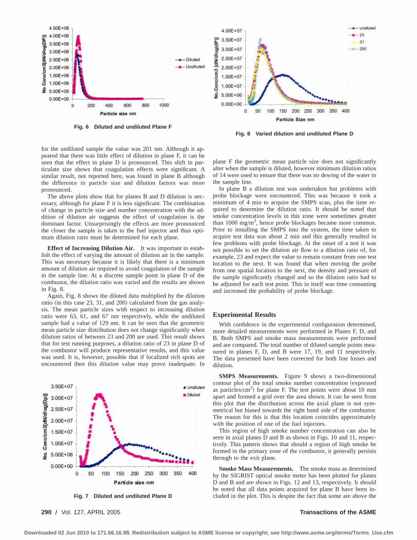
for the undiluted sample the value was 201 nm. Although it ap-peared that there was little effect of dilution in plane F, it can beseen that the effect in plane D is pronounced. This shift in par-ticulate size shows that coagulation effects were significant. Asimilar result, not reported here, was found in plane B althoughthe difference in particle size and dilution factors was morepronounced.

The above plots show that for planes B and D dilution is nec-essary, although for plane F it is less significant. The combinationof change in particle size and number concentration with the ad-dition of dilution air suggests the effect of coagulation is thedominant factor. Unsurprisingly the effects are more pronouncedthe closer the sample is taken to the fuel injector and thus opti-mum dilution ratio must be determined for each plane.

Effect of Increasing Dilution Air. It was important to estab-lish the effect of varying the amount of dilution air in the sample.This was necessary because it is likely that there is a minimumamount of dilution air required to avoid coagulation of the samplein the sample line. At a discrete sample point in plane D of thecombustor, the dilution ratio was varied and the results are shownin Fig. 8.

Again, Fig. 8 shows the diluted data multiplied by the dilutionratio ~in this case 23, 31, and 200! calculated from the gas analy-sis. The mean particle sizes with respect to increasing dilutionratio were 63, 61, and 67 nm respectively, while the undilutedsample had a value of 129 nm. It can be seen that the geometricmean particle size distribution does not change significantly whendilution ratios of between 23 and 200 are used. This result showsthat for test running purposes, a dilution ratio of 23 in plane D ofthe combustor will produce representative results, and this valuewas used. It is, however, possible that if localized rich spots areencountered then this dilution value may prove inadequate. In

plane F the geometric mean particle size does not significantlyalter when the sample is diluted, however minimum dilution ratiosof 14 were used to ensure that there was no dewing of the water inthe sample line.

In plane B a dilution test was undertaken but problems withprobe blockage were encountered. This was because it took aminimum of 4 min to acquire the SMPS scan, plus the time re-quired to determine the dilution ratio. It should be noted thatsmoke concentration levels in this zone were sometimes greaterthan 1000 mg/m3, hence probe blockages became more common.Prior to installing the SMPS into the system, the time taken toacquire test data was about 2 min and this generally resulted infew problems with probe blockage. At the onset of a test it wasnot possible to set the dilution air flow to a dilution ratio of, forexample, 23 and expect the value to remain constant from one testlocation to the next. It was found that when moving the probefrom one spatial location to the next, the density and pressure ofthe sample significantly changed and so the dilution ratio had tobe adjusted for each test point. This in itself was time consumingand increased the probability of probe blockage.

Experimental ResultsWith confidence in the experimental configuration determined,

more detailed measurements were performed in Planes F, D, andB. Both SMPS and smoke mass measurements were performedand are compared. The total number of diluted sample points mea-sured in planes F, D, and B were 17, 19, and 11 respectively.The data presented have been corrected for both line losses anddilution.

SMPS Measurements. Figure 9 shows a two-dimensionalcontour plot of the total smoke number concentration~expressedas particles/cm3! for plane F. The test points were about 10 mmapart and formed a grid over the area shown. It can be seen fromthis plot that the distribution across the axial plane is not sym-metrical but biased towards the right hand side of the combustor.The reason for this is that this location coincides approximatelywith the position of one of the fuel injectors.

This region of high smoke number concentration can also beseen in axial planes D and B as shown in Figs. 10 and 11, respec-tively. This pattern shows that should a region of high smoke beformed in the primary zone of the combustor, it generally persiststhrough to the exit plane.

Smoke Mass Measurements. The smoke mass as determinedby the SIGRIST optical smoke meter has been plotted for planesD and B and are shown in Figs. 12 and 13, respectively. It shouldbe noted that all data points acquired for plane B have been in-cluded in the plot. This is despite the fact that some are above the

Fig. 6 Diluted and undiluted Plane F

Fig. 7 Diluted and undiluted Plane D

Fig. 8 Varied dilution and undiluted Plane D



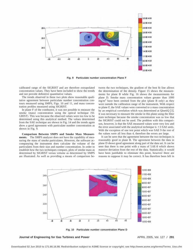
calibrated range of the SIGRIST and are therefore extrapolatedconcentration values. They have been included to show the trendsand not provide definitive quantitative values.

The trends observed in these two plots show reasonable quali-tative agreement between particulate number concentration con-tours measured using SMPS, Figs. 10 and 11, and mass concen-tration profiles measured using SIGRIST.

In plane F of the combustor, it was not possible to measure thesmoke ~mass! concentration using the optical technique~SI-GRIST!. This was because the observed values were too low to bedetermined using this analytical method. The values determinedfrom the SAE technique are shown in Fig. 14 and the trends againshow a good agreement with particulate number concentration asshown in Fig. 9.

Comparison Between SMPS and Smoke Mass Measure-ments. The SMPS analyzer does not have the capability of mea-suring the mass of smoke particulates. However, the software ac-companying the instrument does calculate the volume of theparticulates from their size and number concentration. In order toestablish how the two techniques compare, plots of smoke mass asdetermined by SIGRIST versus volume as determined by SMPSare illustrated. As well as providing a means of comparison be-

tween the two techniques, the gradient of the best fit line allowsthe determination of the density. Figure 15 shows the measure-ments for plane B while Fig. 16 shows the measurements forplane D. Smoke mass concentration values greater than 1000mg/m3 have been omitted from the plot~plane B only! as theywere outside the calibration range of the instrument. With respectto plane F, the SAE values were converted to a mass concentrationby an empirical correlation which was determined at QinetiQ@3#.It was necessary to measure the smoke in this plane using the filterstain technique because the smoke concentration was so low thatthe SIGRIST could not be used. The problem with this compari-son, however, is that the SAE measured values were very low andthe error associated with the analytical technique is63 SAE units.With the exception of one test point which was SAE 9 the rest ofthe values were all less than 4, therefore the errors are large.

It can be seen that the agreement between the two techniques isreasonably good in plane B. The agreement between the data inplane D shows good agreement along part of the data set. It can beseen that there is one point with a mass of 5.6E-8 which showsmassive deviation from the rest of the data. Statistically; it wouldhave been justifiable to eliminate this point, however there arereasons to suppose it may be correct. It has therefore been left in

Fig. 9 Particulate number concentration Plane F

Fig. 10 Particulate number concentration Plane D



Fig. 11 Particulate number concentration Plane B

Fig. 12 Smoke mass mg Õm3 Plane D

Fig. 13 Smoke mass mg Õm3 Plane B



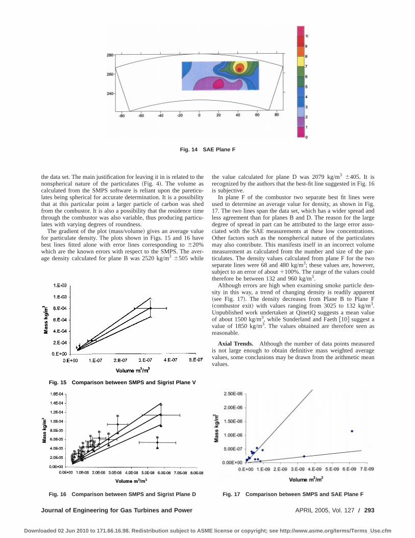
the data set. The main justification for leaving it in is related to thenonspherical nature of the particulates~Fig. 4!. The volume ascalculated from the SMPS software is reliant upon the pareticu-lates being spherical for accurate determination. It is a possibilitythat at this particular point a larger particle of carbon was shedfrom the combustor. It is also a possibility that the residence timethrough the combustor was also variable, thus producing particu-lates with varying degrees of roundness.

The gradient of the plot~mass/volume! gives an average valuefor particulate density. The plots shown in Figs. 15 and 16 havebest lines fitted alone with error lines corresponding to620%which are the known errors with respect to the SMPS. The aver-age density calculated for plane B was 2520 kg/m3 6505 while

the value calculated for plane D was 2079 kg/m3 6405. It isrecognized by the authors that the best-fit line suggested in Fig. 16is subjective.

In plane F of the combustor two separate best fit lines wereused to determine an average value for density, as shown in Fig.17. The two lines span the data set, which has a wider spread andless agreement than for planes B and D. The reason for the largedegree of spread in part can be attributed to the large error asso-ciated with the SAE measurements at these low concentrations.Other factors such as the nonspherical nature of the particulatesmay also contribute. This manifests itself in an incorrect volumemeasurement as calculated from the number and size of the par-ticulates. The density values calculated from plane F for the twoseparate lines were 68 and 480 kg/m3; these values are, however,subject to an error of about1100%. The range of the values couldtherefore be between 132 and 960 kg/m3.

Although errors are high when examining smoke particle den-sity in this way, a trend of changing density is readily apparent~see Fig. 17!. The density decreases from Plane B to Plane F~combustor exit! with values ranging from 3025 to 132 kg/m3.Unpublished work undertaken at QinetiQ suggests a mean valueof about 1500 kg/m3, while Sunderland and Faeth@10# suggest avalue of 1850 kg/m3. The values obtained are therefore seen asreasonable.

Axial Trends. Although the number of data points measuredis not large enough to obtain definitive mass weighted averagevalues, some conclusions may be drawn from the arithmetic meanvalues.

Fig. 14 SAE Plane F

Fig. 15 Comparison between SMPS and Sigrist Plane V

Fig. 16 Comparison between SMPS and Sigrist Plane D Fig. 17 Comparison between SMPS and SAE Plane F



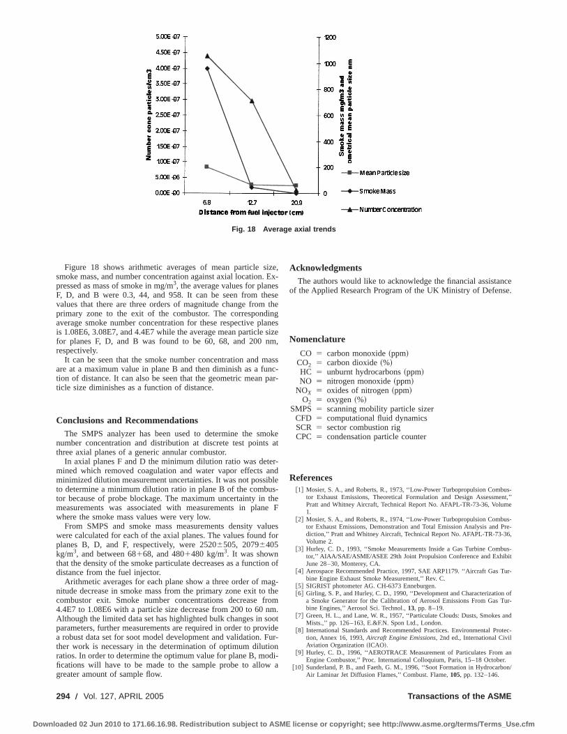
Figure 18 shows arithmetic averages of mean particle size,smoke mass, and number concentration against axial location. Ex-pressed as mass of smoke in mg/m3, the average values for planesF, D, and B were 0.3, 44, and 958. It can be seen from thesevalues that there are three orders of magnitude change from theprimary zone to the exit of the combustor. The correspondingaverage smoke number concentration for these respective planesis 1.08E6, 3.08E7, and 4.4E7 while the average mean particle sizefor planes F, D, and B was found to be 60, 68, and 200 nm,respectively.

It can be seen that the smoke number concentration and massare at a maximum value in plane B and then diminish as a func-tion of distance. It can also be seen that the geometric mean par-ticle size diminishes as a function of distance.

Conclusions and RecommendationsThe SMPS analyzer has been used to determine the smoke

number concentration and distribution at discrete test points atthree axial planes of a generic annular combustor.

In axial planes F and D the minimum dilution ratio was deter-mined which removed coagulation and water vapor effects andminimized dilution measurement uncertainties. It was not possibleto determine a minimum dilution ratio in plane B of the combus-tor because of probe blockage. The maximum uncertainty in themeasurements was associated with measurements in plane Fwhere the smoke mass values were very low.

From SMPS and smoke mass measurements density valueswere calculated for each of the axial planes. The values found forplanes B, D, and F, respectively, were 25206505, 20796405kg/m3, and between 68168, and 4801480 kg/m3. It was shownthat the density of the smoke particulate decreases as a function ofdistance from the fuel injector.

Arithmetic averages for each plane show a three order of mag-nitude decrease in smoke mass from the primary zone exit to thecombustor exit. Smoke number concentrations decrease from4.4E7 to 1.08E6 with a particle size decrease from 200 to 60 nm.Although the limited data set has highlighted bulk changes in sootparameters, further measurements are required in order to providea robust data set for soot model development and validation. Fur-ther work is necessary in the determination of optimum dilutionratios. In order to determine the optimum value for plane B, modi-fications will have to be made to the sample probe to allow agreater amount of sample flow.

AcknowledgmentsThe authors would like to acknowledge the financial assistance

of the Applied Research Program of the UK Ministry of Defense.

Nomenclature

CO 5 carbon monoxide~ppm!CO2 5 carbon dioxide~%!HC 5 unburnt hydrocarbons~ppm!NO 5 nitrogen monoxide~ppm!

NOX 5 oxides of nitrogen~ppm!O2 5 oxygen~%!

SMPS 5 scanning mobility particle sizerCFD 5 computational fluid dynamicsSCR 5 sector combustion rigCPC 5 condensation particle counter

References@1# Mosier, S. A., and Roberts, R., 1973, ‘‘Low-Power Turbopropulsion Combus-

tor Exhaust Emissions, Theoretical Formulation and Design Assessment,’’Pratt and Whitney Aircraft, Technical Report No. AFAPL-TR-73-36, Volume1.

@2# Mosier, S. A., and Roberts, R., 1974, ‘‘Low-Power Turbopropulsion Combus-tor Exhaust Emissions, Demonstration and Total Emission Analysis and Pre-diction,’’ Pratt and Whitney Aircraft, Technical Report No. AFAPL-TR-73-36,Volume 2.

@3# Hurley, C. D., 1993, ‘‘Smoke Measurements Inside a Gas Turbine Combus-tor,’’ AIAA/SAE/ASME/ASEE 29th Joint Propulsion Conference and ExhibitJune 28–30, Monterey, CA.

@4# Aerospace Recommended Practice, 1997, SAE ARP1179. ‘‘Aircraft Gas Tur-bine Engine Exhaust Smoke Measurement,’’ Rev. C.

@5# SIGRIST photometer AG. CH-6373 Enneburgen.@6# Girling, S. P., and Hurley, C. D., 1990, ‘‘Development and Characterization of

a Smoke Generator for the Calibration of Aerosol Emissions From Gas Tur-bine Engines,’’ Aerosol Sci. Technol.,13, pp. 8–19.

@7# Green, H. L., and Lane, W. R., 1957, ‘‘Particulate Clouds: Dusts, Smokes andMists.,’’ pp. 126–163, E.&F.N. Spon Ltd., London.

@8# International Standards and Recommended Practices. Environmental Protec-tion, Annex 16, 1993,Aircraft Engine Emissions, 2nd ed., International CivilAviation Organization~ICAO!.

@9# Hurley, C. D., 1996, ‘‘AEROTRACE Measurement of Particulates From anEngine Combustor,’’ Proc. International Colloquium, Paris, 15–18 October.

@10# Sunderland, P. B., and Faeth, G. M., 1996, ‘‘Soot Formation in Hydrocarbon/Air Laminar Jet Diffusion Flames,’’ Combust. Flame,105, pp. 132–146.

Fig. 18 Average axial trends



K.-U. Schildmacher

R. KochInstitute of Thermal Turbomachinery,

University of Karlsruhe,Kaiserstrasse 12,

76128 Karlsruhe, Germany

Experimental Investigation of theInteraction of Unsteady Flow WithCombustionIn order to reduce the dimensions of the combustor, swirl stabilized flames are used inheavy duty gas turbines. In our recent investigation of the swirling flow at a single heavyduty gas turbine burner under nonreacting conditions typical instabilities like precessingvortex cores and vortex shedding have been found (Schildmacher et al., Proceedings ofthe 6th European Conference on Industrial Furnaces and Boilers). In the present paperthe experimental investigations will be discussed. Combustion instabilities have beenanalyzed by phase-locked laser doppler anemometer measurements. For the reacting flow,also combustion instabilities could be detected. The amplitude increases strongly with theequivalence ratio. The frequency of the oscillations for reacting conditions has been foundto be slightly shifted towards lower frequencies compared to those of the correspondingnonreacting flow. In addition, for the reacting flow a linear and nonlinear range ofoscillations could be discriminated.@DOI: 10.1115/1.1789512#

IntroductionStrong limitations of NOx emissions imposed by legislation

forced the gas turbine industry in recent years to adopt premixedlean combustors which lead to a significant decrease of emissions@1#. However, premixing burners of present gas turbines exceedthe emission level of an ideal premixed flame by a factor of about2 which is mainly to be attributed to nonperfect air-fuel mixing.As pointed out by Kraemer et al.@2#, spatial mixing is quite per-fect in most cases, but temporal fluctuations degrade the mixingquality. These temporal fluctuations of the mixing can be causedby vortex shedding or Kelvin-Helmholtz instabilities@3#.

Although precessing vortex cores and vortex shedding havebeen investigated in a lot of publications of nonreacting swirlingflows @4# not very much is known about the impact of these flowinstabilities on combustion@5#. In order to analyze instabilitymechanisms of the reacting flow in detail, a spatially and time-and phase-resolved flow field analysis using LDA has been per-formed. The oscillating reacting flow was analyzed at differentsound levels. The LDA investigations were supported by pressurefluctuation measurements which where also used to synchronizethe laser doppler anemometer. In the paper, first the transparenttest rig will be described and a short outline of the measurementtechnique will be given. In the main part, the cold flow instabili-ties will be reviewed briefly and then the instabilities of the react-ing flow will be discussed.

BurnerIn this study, a single test burner of industrial size was investi-

gated within an atmospheric test rig~Fig. 1!. It is fired by naturalgas. The burner~Fig. 2! is operated in a combustor casing whichprovides excellent optical access for velocity measurements byLDA. The combustion chamber has a square cross section with atruncated pyramid shape at the exit.

The burner air passage consists of two concentric annular swirl-ers. The inner axial swirler has nozzles for pilot and nonpremixedgas. At the outer diagonal swirler, the gas is injected through holesin the swirler blades in order to enhance premixing with the air.

Burner Operation ConditionsThe burner can be operated either in nonpremixed or premixed

mode @6#. In case of nonpremixed operation, the natural gas isinjected solely through the nonpremixing nozzles. In premixedmode, the premixing gas nozzles and to a minor extent the pilotnozzles are used. In both modes, the air is fed through the axial aswell as through the diagonal swirler passages with the same flowsplit.

In the gas turbine at nominal operation conditions, the burner isoperated in premixed mode with pilot gas injection for betterflame stabilization. Under test rig conditions, the pilot gas injec-tion is not necessary for stable combustion. In order to preventany disturbance of the premixed flame by the pilot burner, no pilotgas was used. In this study, the investigations have been per-formed in premixed mode with a constant air volume flow atatmospheric pressure. The air was pre-heated to 673 K. The Rey-nolds number at the burner mouth was 105 and the thermal powervaried between 420 kW~f50.5! and 810 kW~f50.83!.

Experimental TechniquesThe velocity field was investigated by a two-dimensional~2D!

laser doppler anemometer~LDA ! ~Fig. 3! in back-scatteringmode. The axial and tangential velocities have been recorded inthe x-r plane~Fig. 2!. The air stream was seeded by Al2O3 par-ticles of an average diameter of 1mm. The data rate was 4–20kHz in the main flow and the validation rate was 60–90% for aduration of 20 s per measurement position. Close to the centerwhere the recirculation zone of the flame is located, the data ratedropped sometimes to less than 1 kHz.

In addition, the LDA investigations were accompanied by pres-sure fluctuation measurements. Due to the high temperatures inthe combustion chamber, the quartz pressure sensor was imple-mented into the air plenum of the burner where the air tempera-ture is 673 K. The pressure signal was conditioned by a bandpassfilter of 62.5 Hz half width around the pronounced peak fre-quency at 254 Hz. This filter signal was also used to synchronizethe burst spectrum analyzers of the LDA~Fig. 3!. In contrast tothe nonoscillating flow, the LDA-particle distribution over time isnot uniform. The instantaneous records exhibit a much higher par-ticle rate at moments of high velocities@7#. Thus velocity biasinghad to be taken into account when determining the time-averagedvelocities of the oscillating flow@8,9#.

Contributed by the International Gas Turbine Institute~IGTI! of THE AMERICANSOCIETY OF MECHANICAL ENGINEERSfor publication in the ASME JOURNAL OFENGINEERING FOR GAS TURBINES AND POWER. Paper presented at the Interna-tional Gas Turbine and Aeroengine Congress and Exhibition, Atlanta, GA, June16–19, 2003, Paper No. 2003-GT-38644. Manuscript received by IGTI, Oct. 2002,final revision, Mar. 2003. Associate Editor: H. R. Simmons.



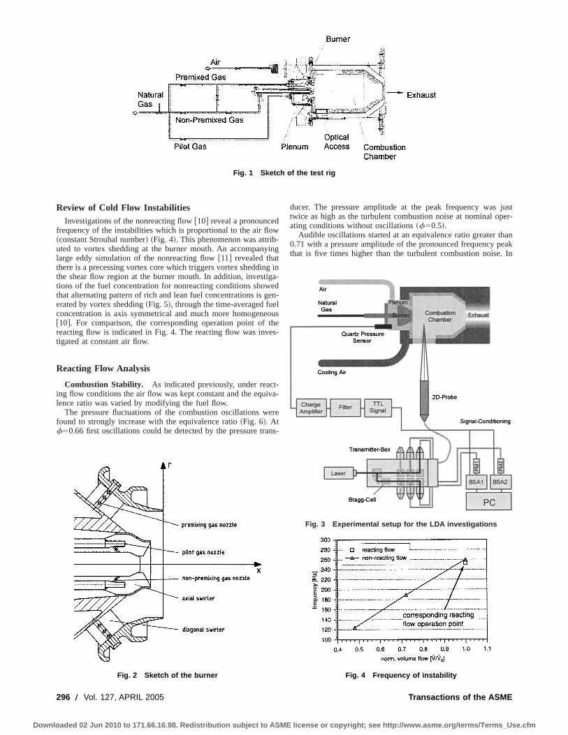
Review of Cold Flow InstabilitiesInvestigations of the nonreacting flow@10# reveal a pronounced

frequency of the instabilities which is proportional to the air flow~constant Strouhal number! ~Fig. 4!. This phenomenon was attrib-uted to vortex shedding at the burner mouth. An accompanyinglarge eddy simulation of the nonreacting flow@11# revealed thatthere is a precessing vortex core which triggers vortex shedding inthe shear flow region at the burner mouth. In addition, investiga-tions of the fuel concentration for nonreacting conditions showedthat alternating pattern of rich and lean fuel concentrations is gen-erated by vortex shedding~Fig. 5!, through the time-averaged fuelconcentration is axis symmetrical and much more homogeneous@10#. For comparison, the corresponding operation point of thereacting flow is indicated in Fig. 4. The reacting flow was inves-tigated at constant air flow.

Reacting Flow Analysis

Combustion Stability. As indicated previously, under react-ing flow conditions the air flow was kept constant and the equiva-lence ratio was varied by modifying the fuel flow.

The pressure fluctuations of the combustion oscillations werefound to strongly increase with the equivalence ratio~Fig. 6!. Atf50.66 first oscillations could be detected by the pressure trans-

ducer. The pressure amplitude at the peak frequency was justtwice as high as the turbulent combustion noise at nominal oper-ating conditions without oscillations~f50.5!.

Audible oscillations started at an equivalence ratio greater than0.71 with a pressure amplitude of the pronounced frequency peakthat is five times higher than the turbulent combustion noise. In

Fig. 1 Sketch of the test rig

Fig. 2 Sketch of the burner

Fig. 3 Experimental setup for the LDA investigations

Fig. 4 Frequency of instability



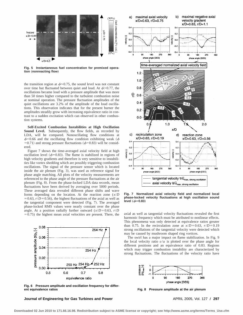
the transition region atf'0.75, the sound level was not constantover time but fluctuated between quiet and loud. Atf.0.77, theoscillations became loud with a pressure amplitude that was morethan 50 times higher compared to the turbulent combustion noiseat nominal operation. The pressure fluctuation amplitudes of thequiet oscillations are 3.2% of the amplitude of the loud oscilla-tions. This observation indicates that for the present burner theamplitudes steadily grow with increasing equivalence ratio in con-trast to a sudden excitation which can observed in other combus-tion systems.

Self-Excited Combustion Instabilities at High OscillationSound Level. Subsequently, the flow fields, as recorded byLDA, will be compared. Nonoscillating flow conditions atf50.66 and the oscillating flow condition exhibiting weak~f50.71! and strong pressure fluctuations~f50.83! will be consid-ered.

Figure 7 shows the time-averaged axial velocity field at highoscillation level~f50.83!. The flame is stabilized in regions ofhigh velocity gradients and therefore is very sensitive to instabili-ties like vortex shedding which are possibly triggering combustionoscillations. The signal of the pressure sensor which is locatedinside the air plenum~Fig. 3!, was used as reference signal forphase angle matching. All plots of the velocity measurements arereferenced to the phase angle of the pressure fluctuations at the airplenum~Fig. 8!. From the phase-locked LDA data records, meanfluctuations have been derived by averaging over 5000 periods.These averaged data revealed different phase shifts and waveforms depending on the location. At the reaction zone (x/D50.63,r /D50.56), the highest fluctuations of the axial as well asthe tangential component were detected~Fig. 7!. The averagedphase-locked RMS values were nearly constant over the phaseangle. At a position radially further outward (x/D50.63, r /D50.75) the highest mean axial velocities are present. There, theaxial as well as tangential velocity fluctuations revealed the first

harmonic frequency which must be attributed to nonlinear effects.This phenomena was only detected at equivalence ratios greaterthan 0.75. In the recirculation zone atx/D50.63, r /D50.19strong oscillations of the tangential velocity were detected whichmay be caused by mushroom shaped ring vortices.

The swirl has a major impact on flame stabilization. In Fig. 9the local velocity ratiov/u is plotted over the phase angle fordifferent positions and an equivalence ratio of 0.83. Regionswhich may trigger combustion instability are characterized bystrong fluctuations. The fluctuations of the velocity ratio have

Fig. 5 Instantaneous fuel concentration for premixed opera-tion „nonreacting flow …

Fig. 6 Pressure amplitude and oscillation frequency for differ-ent equivalence ratios

Fig. 7 Normalized axial velocity field and normalized localphase-locked velocity fluctuations at high oscillation soundlevel „fÄ0.83…

Fig. 8 Pressure amplitude at the air plenum



been analyzed on basis of the LDA data. The data reveal, thestrongest fluctuation of 0.1<v/u<0.8 are found in the reactionzone (x/D50.63, r /D50.56). Because of the periodicity of thesignal, the fluctuations must be attributed to coherent structures.The plot also indicates that for a short time at around 150 degphase angle, swirl stabilization of the flame is interrupted whichmay cause to strong strain rates in the reaction zone and localflame quenching. Outside the recirculation zone only minor fluc-tuations of the velocity ratio were recorded.

Self-Excited Combustion Instabilities at Low OscillationSound Level. For an equivalence ratio off50.71 barely au-dible oscillations have been detected. The amplitude of the pres-sure oscillations was more than thirty times smaller compared tostrong oscillations but five times higher than the turbulent com-bustion noise~Fig. 6!. Figure 10 shows the flow field and thephase-locked velocity fluctuations at different positions. Every-where inside the combustion chamber the frequency of the veloc-ity fluctuations was identical to that of the pressure oscillations.Higher harmonic frequencies amplitude compared to operation athigh oscillation level, the velocity fluctuations were reduced onlyby a factor of 4.

The velocity ratiov/u only varied between 0.35 and 0.5~Fig.11!, and due to the reduced strain rate the flame was more stable.

Fluctuations Close to the Onset of Combustion Oscilla-tion. As stated previously, the first onset of combustion oscilla-tions was detected at an equivalence ratio of 0.66. The time-averaged velocity field atf50.66 was quite similar to that of theweakly oscillating flow atf50.71.

Due to the small amplitude of the pressure oscillations that wasjust twice as high as the turbulent combustion noise, it was notpossible to generate a useful trigger signal for synchronization ofthe burst spectrum analyzers. Therefore subsequently frequencyspectra will be used for the analysis. For extracting the spectraldata, the resampling method was adopted@12,13#.

The frequency spectra of the local axial and tangential veloci-ties are shown in Fig. 12. Generally, a pronounced frequency peakwas not found for the stable operating conditions. Very small sinu-soidal velocity fluctuations at about 254 Hz could only be detectedin the axial component at regions of high velocities (x/D50.37,r /D50.56). Comparing the spectra obtained for the reacting case~Fig. 12! to those of the corresponding nonreacting flow case, thecoherent flow structures which are present in the nonreacting flowand which cause the pronounced frequency peak at 263 Hz are notreproduced under reacting flow conditions.

Moreover, even in the flow field upstream of the reaction zone~e.g.,x/D50.37,r /D50.56) no fluctuations are present. This em-phasizes the strong impact of the heat release on the generation ofcoherent flow structures. This observation is also confirmed byFig. 13. The frequency and the corresponding Strouhal number

Fig. 9 Phase-locked velocity ratio v Õu at high pressure fluc-tuations

Fig. 10 Normalized axial velocity field and normalized localphase-locked velocity fluctuations at low oscillation soundlevel „fÄ0.71…

Fig. 11 Phase-locked velocity ratio v Õu at low pressure fluc-tuations



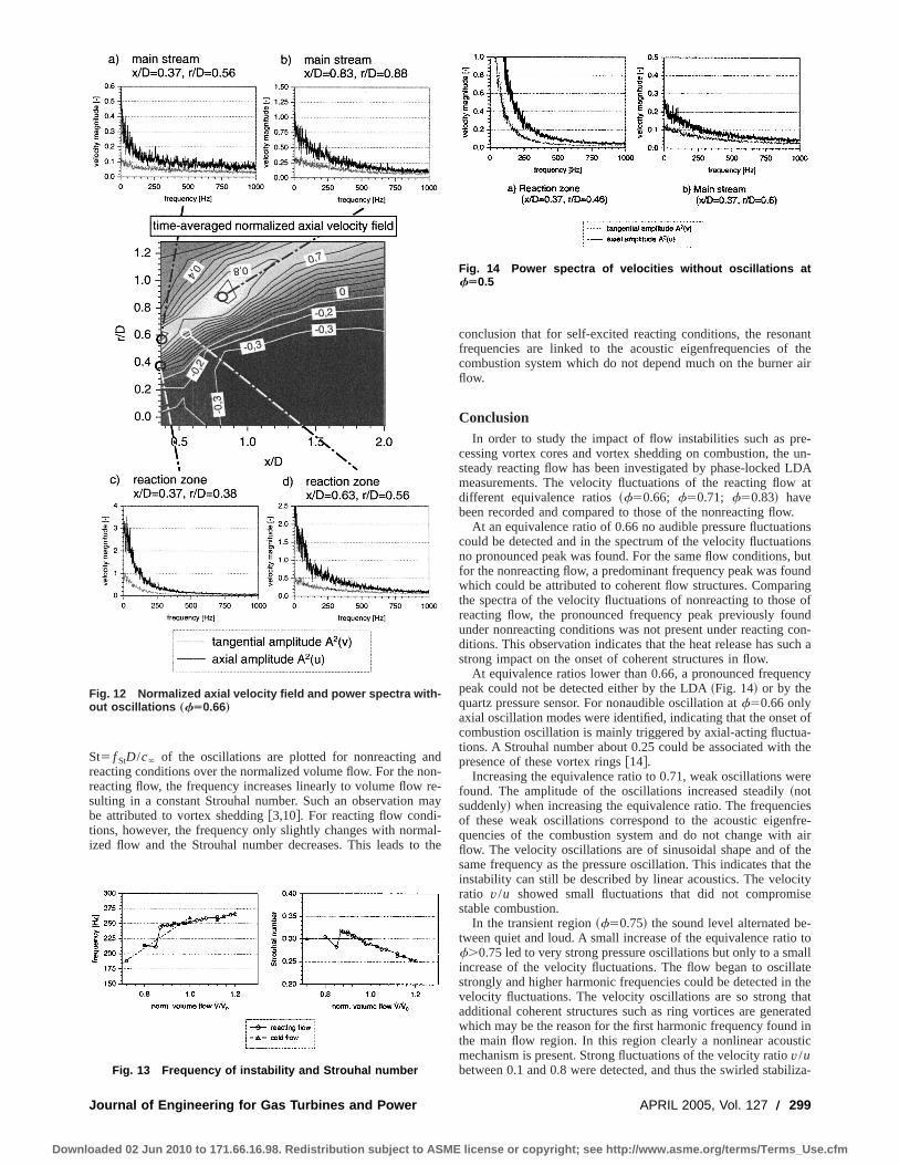
St5 f StD/c` of the oscillations are plotted for nonreacting andreacting conditions over the normalized volume flow. For the non-reacting flow, the frequency increases linearly to volume flow re-sulting in a constant Strouhal number. Such an observation maybe attributed to vortex shedding@3,10#. For reacting flow condi-tions, however, the frequency only slightly changes with normal-ized flow and the Strouhal number decreases. This leads to the

conclusion that for self-excited reacting conditions, the resonantfrequencies are linked to the acoustic eigenfrequencies of thecombustion system which do not depend much on the burner airflow.

ConclusionIn order to study the impact of flow instabilities such as pre-

cessing vortex cores and vortex shedding on combustion, the un-steady reacting flow has been investigated by phase-locked LDAmeasurements. The velocity fluctuations of the reacting flow atdifferent equivalence ratios~f50.66; f50.71; f50.83! havebeen recorded and compared to those of the nonreacting flow.

At an equivalence ratio of 0.66 no audible pressure fluctuationscould be detected and in the spectrum of the velocity fluctuationsno pronounced peak was found. For the same flow conditions, butfor the nonreacting flow, a predominant frequency peak was foundwhich could be attributed to coherent flow structures. Comparingthe spectra of the velocity fluctuations of nonreacting to those ofreacting flow, the pronounced frequency peak previously foundunder nonreacting conditions was not present under reacting con-ditions. This observation indicates that the heat release has such astrong impact on the onset of coherent structures in flow.

At equivalence ratios lower than 0.66, a pronounced frequencypeak could not be detected either by the LDA~Fig. 14! or by thequartz pressure sensor. For nonaudible oscillation atf50.66 onlyaxial oscillation modes were identified, indicating that the onset ofcombustion oscillation is mainly triggered by axial-acting fluctua-tions. A Strouhal number about 0.25 could be associated with thepresence of these vortex rings@14#.

Increasing the equivalence ratio to 0.71, weak oscillations werefound. The amplitude of the oscillations increased steadily~notsuddenly! when increasing the equivalence ratio. The frequenciesof these weak oscillations correspond to the acoustic eigenfre-quencies of the combustion system and do not change with airflow. The velocity oscillations are of sinusoidal shape and of thesame frequency as the pressure oscillation. This indicates that theinstability can still be described by linear acoustics. The velocityratio v/u showed small fluctuations that did not compromisestable combustion.

In the transient region~f50.75! the sound level alternated be-tween quiet and loud. A small increase of the equivalence ratio tof.0.75 led to very strong pressure oscillations but only to a smallincrease of the velocity fluctuations. The flow began to oscillatestrongly and higher harmonic frequencies could be detected in thevelocity fluctuations. The velocity oscillations are so strong thatadditional coherent structures such as ring vortices are generatedwhich may be the reason for the first harmonic frequency found inthe main flow region. In this region clearly a nonlinear acousticmechanism is present. Strong fluctuations of the velocity ratiov/ubetween 0.1 and 0.8 were detected, and thus the swirled stabiliza-

Fig. 12 Normalized axial velocity field and power spectra with-out oscillations „fÄ0.66…

Fig. 13 Frequency of instability and Strouhal number

Fig. 14 Power spectra of velocities without oscillations atfÄ0.5



tion of the flame was disturbed periodically for a short time. Thismechanism seems to have a major impact on the combustion sta-bility.

AcknowledgmentThis study was supported by the EC under contract ENK5-CT-

2000-00060~PRECCINSTA! which is gratefully acknowledged.

Nomenclature

A 5 amplitude, magnitudeBSA 5 burst spectrum analyzer

c 5 velocityc` 5 axial velocity at the burner exitD 5 burner outlet diameterf 5 frequency

f St 5 Strouhal frequencyp 5 pressure

PM1,PM2 5 photomultiplier

r 5 radial directionRMS 5 root-mean-square value

St 5 Strouhal numberu 5 axial velocityV 5 volume flowv 5 tangential velocityx 5 axial directiony 5 normal directionf 5 equivalence ratio

Subscripts

0 5 nominal operation, design pointmax 5 maximum

Superscripts

¯ 5 time-averaged component˜ 5 periodical component

) 5 turbulent component

References@1# Lefebvre, A. H., 1974, ‘‘Pollution Control in Continuous Combustion En-

gines,’’ Fifteenth Symposium on Combustion, Combustion Inst., Pittsburgh,pp. 1169–1180.

@2# Kraemer, H., Dinkelacker, F., Huth, M., Leipertz, A., Poeschl, G., and Lenze,M., 1999, ‘‘Optimization of the Mixing Quality of a Real Size Gas TurbineBurner With Instantaneous Planar Laser-Induced Fluorescence Imaging,’’ASME Paper No. 99-GT-135.

@3# Coats, C. M., 1996, ‘‘Coherent Structures in Combustion,’’ Prog. Energy Com-bust. Sci.,22, pp. 427–509.

@4# Gupta, A. K., Lilley, D. G., and Syred, N., 1984, ‘‘Swirl Flows,’’ ABACUSPress.

@5# Gutmark, E. J., Shadow, K. C., and Yu, K. H., 1994, ‘‘Methods for EnhancedTurbulence Mixing in Supersonic Shear Flows,’’ Appl. Mech. Rev.,47~2!, pp.375–417.

@6# Prade, B., Streb, H., Berenbrink, P., Schetter, B., and Pyka, G., 1996, ‘‘Devel-opment of an Improved Hybrid Burner—Initial Operating Experience in a GasTurbine,’’ ASME Paper No. 96-GT-43.

@7# Schildmacher, K.-U., Koch, R., Krebs, W., Hoffmann, S., and Wittig, S., 2002,‘‘Experimental Investigation of Unsteady Flow Phenomena in High IntenseCombustion Systems,’’Proceedings of the 6th European Conference on Indus-trial Furnaces and Boilers.

@8# Loseke, A. H., and Gould, R. D., 1991, ‘‘A Comparison of Velocity BiasCorrection Techniques in Laser-Doppler-Velocimetry,’’ ASME Fluid Measure-ment and Instrumentation Forum,108, pp. 63–68.

@9# McLaughlin, D. K., and Tiedermann, W. G., 1973, ‘‘Biasing Correction forIndividual Realization of Laser-Doppler-Anemometer Measurements in Turbu-lent Flow,’’ The Physics of Flow,16, pp. 2082–2088.

@10# Schildmacher, K.-U., Koch, R., Krebs, W., Hoffmann, S., and Wittig, S., 2000,‘‘Experimental Investigations of the Temporal Air-Fuel Mixing Fluctuationsand Cold Flow Instabilities of a Premixing Gas Turbine Burner,’’ ASME PaperNo. 2000-GT-0084.

@11# Schlueter, J., Schoenfeld, T., Poinsot, T., Krebs, W., and Hoffmann, S., 2001,‘‘Characterization of Confined Swirl Flows Using Large Eddy Simulations,’’ASME Paper No. 2001-GT-0060.

@12# Host-Madsen, A., 1994, ‘‘A New Method for Estimation of Turbulence Spectrafor Laser Doppler Anemometry,’’ 7th International Symposium on Applica-tions of Laser Techniques of Fluid Mechanics, Lisbon.

@13# Host-Madsen, A., and Caspersen, C., 1981, ‘‘Spectral Analysis—A ModernPerspective,’’ Proc. IEEE,69~11!, pp. 1380–1419.

@14# Laufer, J., and Monkewitz, P., 1978, ‘‘The Influence of the Dominant LargeScale Structures on the Initial Instability of a Low-Speed Circular Jet,’’ Bull.Am. Phys. Soc.,23, p. 1008.



J. Eckstein

E. Freitag

C. Hirsch

T. Sattelmayer

Lehrstuhl fur Thermodynamik,Technische Universitat Munchen,

85747 Garching,Germany

R. von der Bank

T. Schilling

Rolls-Royce Deutschland Ltd. & Co. KG,Combustor Aerodynamics,

Eschenweg 11,15827 Dahlewitz, Berlin, Germany

Forced Low-Frequency SprayCharacteristics of a GenericAirblast Swirl Diffusion BurnerThe low-frequency response of the spray from a generic airblast diffusion burner with adesign typical of an engine system has been investigated as part of an experimental studyto describe the combustion oscillations of aeroengine combustors called rumble. Theatomization process was separated from the complex instability mechanism of rumble byusing sinusoidal forcing of the air mass flow rate without combustion. Pressure dropacross the burner and the velocity on the burner exit were found to follow the steadyBernoulli equation. Phase-locked particle image velocimetry measurements of the forcedvelocity field of the burner show quasisteady behavior of the air flow field. The phase-locked spray characteristics were measured for different fuel flow rates. Here again quasi-steady behavior of the atomization process was observed. With combustion, the phase-locked Mie-scattering intensity of the spray cone was found to follow the spray behaviormeasured in the noncombusting tests. These findings lead to the conclusion that theunsteady droplet Sauter mean diameter mean and amplitude of the airblast atomizer canbe calculated using the steady-state atomization correlations with the unsteady burner airvelocity. @DOI: 10.1115/1.1789515#

IntroductionThe demand for significant reductions of pollutant emissions

like NOx and smoke from gas turbine aeroengines has motivatedcontinuous improvement of the combustion processes within theconstraints of the engine operation. New concepts of fuel atomi-zation, pre-vaporization, and staged injection have been devel-oped or are currently being tested for their operability. However,with the improvements gained, thermoacoustic combustion insta-bilities known and feared for their destructive potential in station-ary gas turbines have also become more prominent in aeroengines.During recent years intense scientific efforts were undertaken tounderstand and specify the underlying driving mechanisms~e.g.,Refs. @1–3#!. A particular combustion instability of aeroenginecombustors is related to the fuel spray atomizers used. It exhibitsa low-frequency oscillation between 50 and 150 Hz at idle andsubidle conditions, commonly called ‘‘rumble.’’ In engine designpractice, certain atomizers or combinations of fuel injector andcombustor have become known as being particularly rumbleprone, yet a standard procedure to predict and to prevent a givendesigns susceptibility to this kind of instability has still to beformulated @4#. Work in this area was performed by Zhu et al.who formulated a computational fluid dynamics~CFD! model tonumerically simulate the response of a two-dimensional~2D!model combustor to forcing of the fuel and air streams@5# as wellas the onset of self-excited oscillation@6#. In this paper we pro-vide the experimental results which clarify one of the key mecha-nisms of the rumble instability, i.e., the fuel atomization. A ge-neric airblast atomizer with a design typical for current systemshas been incorporated into a thermoacoustic combustor test rigsimulating rumble conditions. To isolate the effect of acousticoscillation upon the atomization, the forced response of the atom-izer has been investigated under noncombustion conditions.Phase-locked measurements of the pressure velocity coupling atthe burner, the combustor velocity field, as well as the associated

spray diameter spectra were taken to provide a clear picture of theunsteady atomization process. The conclusions were verified us-ing Mie scattering of the spray cone in the combusting environ-ment. For all measurements, a periodically forced air flow in thefrequency range 50–150 Hz was provided at different mean airmass flows~AMFs! and fuel mass flows~FMFs!, covering thetypical range of rumble.

Experimental SetupIn this section, the experimental setup, the measurement tech-

niques and the error estimates pertaining to the data presented inthe results section are being presented. Also, the operational pa-rameters of the experiments are given.

Test Facility. The single sector test rig, in which the measure-ments were conducted under atmospheric pressure conditions, issketched in Fig. 1. Harmonic forcing on the electrically pre-heatedair flow is created by a siren. The siren works on the principle ofa rotating disc in an axial flow. The rotor has rectangular orificespassing double sine shaped apertures on the stator plate. Practicehas shown that a sinusoidal excitation is well achieved if the airleakages around the rotor are kept small. The siren is driven by a1.1-kW induction motor. The rotation speed is controlled by afrequency converter, producing excitation frequencies up to 850Hz. In order to adjust the excitation amplitudes, the siren unit hasa bypass valve, which allows the alteration of the air mass flowratio between the siren and the bypass passage.

A supply tube connects the siren to the combustion chamber.The supply tube has a circular cross section with 124-mm innerdiameter, and its length is adjustable from 850 to 1450 mm. In thisway tube resonance effects may be used or avoided to furthercontrol the forcing amplitude. For the measurements presentedhere the maximum supply tube length was used. The acoustics ofthe supply were shown to be 1D using the ten equally spacedmicrophone ports in the far field of the siren. The supply tube andthe combustion chamber are connected with an adapter piece ac-commodating the injector/burner investigated. A thermocouplegives the air temperature at the injector inlet. The mean and os-cillating pressure drop over the injector are determined by corre-sponding pairs of pressure taps and microphone ports close to theburner inlet and outlet planes.




The combustion chamber has a square cross section, and mea-sures 903903300 mm. Exchangeable side plates allow a flexibleadaptation to the requirements of the measurement techniques ap-plied. The primary combustion zone is optically accessible byexchangeable quartz windows. A hot-wire probe can be mounted 3mm downstream of the burner outlet for the determination of theacoustic velocities. Ignition is achieved using a spark plug. For thecombustion chamber, an acoustic open end condition can be as-sumed, since the exhaust tube measures 500 mm in diameter anddoes not contain a silencer.

The generic airblast diffusion injector/combustor system inves-tigated is of the rich-quench-lean type, such that holes for second-ary air injection were provided in the top and bottom plates of thecombustion chamber, meeting the aerodynamic and stoichiometricoperating conditions. The hole pattern and location was derivedfrom the real~annular! liner geometry. The hole diameters weredetermined from the original air distribution on the basis of CFD.The air flow through these holes is diverted from the main flowupstream of the siren valve and is controlled by a flow restrictorvalve with a corresponding measurement orifice. Dilution, filmand liner cooling in the downstream part of the combustion cham-ber were omitted since they do not contribute to the formation ofthe primary zone aimed at in the current investigation.

Measurement Techniques and Data Analysis. A major re-quirement in the current experiments is to capture phase lockeddata. For this the siren shaft provides a reference signal, such thatthe exact forcing frequency and the phase angle of all measure-ments relative to the forcing can be determined. For the time-resolved measurement of the acoustic velocity, a 5-mm constanttemperature anemometer~CTA! hot-wire probe has been used. Itwas located 3 mm downstream of the injector exit in the horizon-tal centerplane of the combustion chamber. The position of theprobe was chosen such that the maximum velocity and at the sametime a low local turbulence level was obtained, to make the mea-surement representative of the acoustic burner velocity. Addition-ally, the dynamic pressure drop over the burner has been measuredby means of two1

4-in. microphones being located directly up-stream and downstream of the burner. The acquisition of theacoustic data~pressures and velocities! is controlled by amultichannel-I/O board~300 kHz, 12 bit!. The microphone chan-nels and the CTA channel were sampled with 10 kHz each. Time-domain sequences of 10,000 samples each were taken and Fouriertransformed. Then the amplitude and phase of each signal at theforcing frequency were stored. Finally, the averages were com-puted for all measurement sets from a given operating condition.The errors of the CTA velocity measurements are estimated to bebelow63.5% relative error and those of the microphone pressureamplitudes to be below65% relative error.

Phase-locked PIV and spray measurements were obtained bymeans of a hardware trigger. The rectangular reference signal is

used to start a programmable counter on a PCI board, which trig-gers the measurement devices on completion of the preselectedcountdown.

Particle Image Velocimetry (PIV).PIV was employed to de-termine the flow field in the central longitudinal section of thecombustion chamber. For detailed data at the combustor outlet, aregion in the vicinity of the injector exit was investigated whichmeasured 20332 mm starting 1 mm downstream of the combus-tor front as shown in Fig. 2. 100 vector maps were recorded andaveraged to obtain the flow field data at every measured phaseangle. The recording of the air velocity field took place withoutspray and flame. Oil droplets were used as seeding. The PIV light-sheet was also used for spray visualization by Mie scattering.Comparison of the PIV data with CTA data of corresponding casesleads to a relative error estimate of about63% of the measuredvelocity.

Malvern Particle Sizing. The Spraytec Particle Sizer was usedto characterize the spray at the injector exit under nonignited con-ditions. The measurement volume made up by the laser beam hada diameter of 15 mm and was located at a distance of 12 mmdownstream of the injector exit in the horizontal center plane ofthe combustor~see Fig. 2!. The recordings have been performedphase triggered, taking 1250 samples at a sampling frequency of2.5 kHz. For the ambient temperature spray measurements, re-peatability and consistency checks make the SMD size measure-ments rather reliable. At elevated temperatures, beam steeringcaused by density gradients may introduce a considerable sourceof error. Again repeatability and consistency were checked, e.g.,by comparing the measured temperature dependence of the SMDwith the temperature scalings known from literature@7#. From thetypical data scatter an error bar of65% is estimated for the SMDmeasurements.

Operating Conditions. The measurement points were de-rived from the startup operating conditions of the real combustor.They are characterized by low pressures inside the combustionchamber~1.2–3.6 bars!, moderate air temperatures~maximum430 K! and low AFR’s in the combustion zone~18–40, withoutdilution!. Since measurements were to be performed at ambientpressure, the preheating temperatures were maintained and the airand fuel mass flows were adapted such that the AFR of the pri-mary zone and the characteristic pressure losses over the burnerwere retained. For the spray measurements without combustion, amixture of 90% ethanol and 10% water was used as fuel which

Fig. 1 „Color online … Schematic representation of the test rigFig. 2 „Color online … Schematic representation of the positionof the PIV-investigation area „light gray … and the Malvern laserbeam „dark gray … in the vertical center plane of the combustionchamber relative to the injector outlet



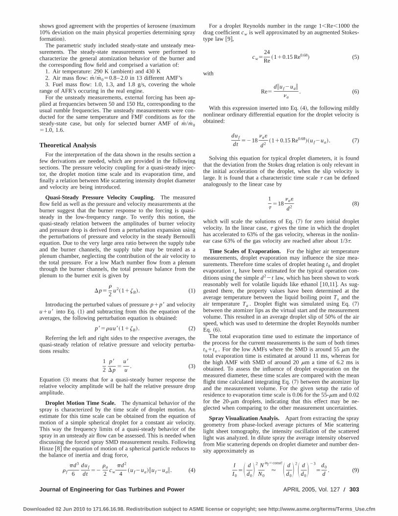
shows good agreement with the properties of kerosene~maximum10% deviation on the main physical properties determining sprayformation!.

The parametric study included steady-state and unsteady mea-surements. The steady-state measurements were performed tocharacterize the general atomization behavior of the burner andthe corresponding flow field and comprised a variation of:

1. Air temperature: 290 K~ambient! and 430 K2. Air mass flow:m/m050.8– 2.0 in 13 different AMF’s3. Fuel mass flow: 1.0, 1.3, and 1.8 g/s, covering the whole

range of AFR’s occuring in the real engine.For the unsteady measurements, external forcing has been ap-

plied at frequencies between 50 and 150 Hz, corresponding to theusual rumble frequencies. The unsteady measurements were con-ducted for the same temperature and FMF conditions as for thesteady-state case, but only for selected burner AMF ofm/m051.0, 1.6.

Theoretical AnalysisFor the interpretation of the data shown in the results section a

few derivations are needed, which are provided in the followingsections. The pressure velocity coupling for a quasi-steady injec-tor, the droplet motion time scale and its evaporation time, andfinally a relation between Mie scattering intensity droplet diameterand velocity are being introduced.

Quasi-Steady Pressure Velocity Coupling. The measuredflow field as well as the pressure and velocity measurements at theburner suggest that the burner response to the forcing is quasi-steady in the low-frequency range. To verify this notion, thequasi-steady relation between the amplitudes of burner velocityand pressure drop is derived from a perturbation expansion usingthe perturbations of pressure and velocity in the steady Bernoulliequation. Due to the very large area ratio between the supply tubeand the burner channels, the supply tube may be treated as aplenum chamber, neglecting the contribution of the air velocity tothe total pressure. For a low Mach number flow from a plenumthrough the burner channels, the total pressure balance from theplenum to the burner exit is given by

Dp5r

2u2~11zB!. (1)

Introducing the perturbed values of pressurep1p8 and velocityu1u8 into Eq. ~1! and subtracting from this the equation of theaverages, the following perturbation equation is obtained:

p85ruu8~11zB!. (2)

Referring the left and right sides to the respective averages, thequasi-steady relation of relative pressure and velocity perturba-tions results:

1

2

p8

Dp5

u8

u. (3)

Equation~3! means that for a quasi-steady burner response therelative velocity amplitude will be half the relative pressure dropamplitude.

Droplet Motion Time Scale. The dynamical behavior of thespray is characterized by the time scale of droplet motion. Anestimate for this time scale can be obtained from the equation ofmotion of a simple spherical droplet for a constant air velocity.This way the frequency limits of a quasi-steady behavior of thespray in an unsteady air flow can be assessed. This is needed whendiscussing the forced spray SMD measurement results. FollowingHinze @8# the equation of motion of a spherical particle reduces tothe balance of inertia and drag force,

r f

pd3

6

duf

dt52

ra

2cw

pd2

4~uf2ua!iuf2uai . (4)

For a droplet Reynolds number in the range 1,Re,1000 thedrag coefficientcw is well approximated by an augmented Stokes-type law @9#,

cw524

Re~110.15 Re0.68! (5)

with

Re5diuf2uai

na. (6)

With this expression inserted into Eq.~4!, the following mildlynonlinear ordinary differential equation for the droplet velocity isobtained:

duf

dt5218

na«

d2~110.15 Re0.68!~uf2ua!. (7)

Solving this equation for typical droplet diameters, it is foundthat the deviation from the Stokes drag relation is only relevant inthe initial acceleration of the droplet, when the slip velocity islarge. It is found that a characteristic time scalet can be definedanalogously to the linear case by

1

t518

na«

d2(8)

which will scale the solutions of Eq.~7! for zero initial dropletvelocity. In the linear case,t gives the time in which the droplethas accelerated to 63% of the gas velocity, whereas in the nonlin-ear case 63% of the gas velocity are reached after about 1/3t.

Time Scales of Evaporation. For the higher air temperaturemeasurements, droplet evaporation may influence the size mea-surements. Therefore time scales of droplet heatingth and dropletevaporationtv have been estimated for the typical operation con-ditions using the simpled22t law, which has been shown to workreasonably well for volatile liquids like ethanol@10,11#. As sug-gested there, the property values have been determined at theaverage temperature between the liquid boiling pointTs and theair temperatureTa . Droplet flight was simulated using Eq.~7!between the atomizer lips as the virtual start and the measurementvolume. This resulted in an average droplet slip of 50% of the airspeed, which was used to determine the droplet Reynolds numberEq. ~6!.

The total evaporation time used to estimate the importance ofthe process for the current measurements is the sum of both timesth1tv . For the low AMFs where the SMD is around 55mm thetotal evaporation time is estimated at around 11 ms, whereas forthe high AMF with SMD of around 20mm a time of 6.2 ms isobtained. To assess the influence of droplet evaporation on themeasured diameter, these time scales are compared with the meanflight time calculated integrating Eq.~7! between the atomizer lipand the measurement volume. For the given setup the ratio ofresidence to evaporation time scale is 0.06 for the 55-mm and 0.02for the 20-mm droplets, indicating that this effect may be ne-glected when comparing to the other measurement uncertainties.

Spray Visualization Analyis. Apart from extracting the spraygeometry from phase-locked average pictures of Mie scatteringlight sheet tomography, the intensity oscillation of the scatteredlight was analyzed. In dilute spray the average intensity observedfrom Mie scattering depends on droplet diameter and number den-sity approximately as

I

I 05S d

d0D 2 N

N0'

mf5const!S d

d0D 2S d

d0D 23

5d0

d. (9)



For a constant fuel mass flow rate, the particle number ratio inthe second term of Eq.~9! can be expressed by droplet diameter.For the current atomizer under steady-state conditions the dropletdiameter and air velocity correlate well with

d

d05S ua,0

uaD j

, j.1. (10)

Given Eqs.~10! and ~9!, the measured intensity amplitude canbe transformed into a velocity amplitude,

ua8

ua,05

1

j

I 8

I 0. (11)

With this equation and given the steady atomizer characteris-tics, relative velocity amplitudes may be calculated from relativeMie intensity amplitudes for quasisteady behavior of the atomizer.Thus it provides an easy check for quasi-steady spray behavior.

Results

Pressure Velocity Coupling Under Forcing. In Fig. 3, thecomparison of the amplitudes of half the relative pressure droposcillation measured with microphones and the relative velocityoscillation measured with the hot wire are compared for threemean flowrates: 1, 1.3, and 1.6 times the reference air mass flowrate.

The correlation between the relative velocity amplitude and halfthe relative pressure amplitude is very good. Therefore Eq.~3!holds, which means that the burner flow responds quasi-steady tothe low-frequency forcing. The small differences observed be-tween velocity and pressure amplitudes, seen in particular for thehigher frequencies at the lowest flow rate (p8/2p and u8/u form/m051), decrease with increasing flow rate. This is due to thesignal-to-noise ratio of the CTA which improves with mean ve-locity. For increasing flow rate the relative amplitudes achieved atthe burner are seen to decrease, because the rising burner backpressure reduces the relative forcing amplitude.

Velocity Field Under Forcing. Figure 4 shows the velocitydistribution at the burner exit for a forcing at 90 Hz. On the lefthalf of the picture, the contour lines represent two fixed levels ofair velocity magnitude at ten different phase angles with a phaseseparation ofDw536. The spread of the superposed contoursgives an impression of the injector’s velocity response and showshow the swirling jet velocity grows and diminishes during theforcing period.

On the right half of Fig. 4 the contourlines of equal relativevelocity are shown. These are obtained by normalizing the localphase-averaged velocities with the injector exit velocity of therespective phase angle. The contours coincide, meaning that the

velocity field is invariant during the forcing cycle. Therefore theaerodynamic behavior of the injector is quasi-steady for the fre-quency range considered, which is in line with the pressure-velocity coupling discussed above.

Stationary Atomization Measurements. Figure 5 shows themeasured SMD of the burner for different AMF’s and two airtemperatures. As typical for airblast atomizers, the SMD is domi-nated by the air mass flow rate and relative atomization velocitiesat the atomizer lip. For relative AMF.1.5 and low viscosity fuel,the atomization process is solely governed by the Weber numberWe. Referring to the relation given in Ref.@7#:

SMD

Lc}We2x. (12)

For the current data an exponentx'0.8 with respect to theAMF variation andx'0.5 for the temperature change is obtained.This is in agreement with the typical values for air blast atomizersfound in the literature@7,12#. A possible reason for the differentvalues ofx may be secondary spray breakup. With decreasingrelative AMF,1.5 the disruptive forces decrease strongly, whichtends to decrease the slope of the curve in this range. According tothe stationary curves in Figs. 6 and 7, the SMD is fairly insensi-tive to changing FMF, giving only a 10% diameter increase foralmost double fuel flow rate.

Fig. 3 „Color online … Comparison of measured pressure am-plitudes „symbols … and velocities „lines … over frequency forthree mass flow rates in a noncombusting environment

Fig. 4 Phase-locked velocity field at 90 Hz without combus-tion: the left half shows two contour levels of velocity magni-tude for all ten phase angles, the right half shows the samefield scaled with the average velocity at the burner exit

Fig. 5 „Color online … SMD over relative AMF for different pre-heating temperatures in the stationary, noncombusting case



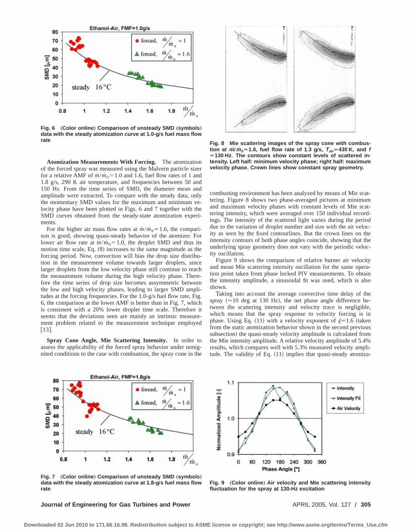
Atomization Measurements With Forcing. The atomizationof the forced spray was measured using the Malvern particle sizerfor a relative AMF ofm/m051.0 and 1.6, fuel flow rates of 1 and1.8 g/s, 290 K air temperature, and frequencies between 50 and150 Hz. From the time series of SMD, the diameter mean andamplitude were extracted. To compare with the steady data, onlythe momentary SMD values for the maximum and minimum ve-locity phase have been plotted in Figs. 6 and 7 together with theSMD curves obtained from the steady-state atomization experi-ments.

For the higher air mass flow rates atm/m051.6, the compari-son is good, showing quasi-steady behavior of the atomizer. Forlower air flow rate atm/m051.0, the droplet SMD and thus itsmotion time scale, Eq.~8! increases to the same magnitude as theforcing period. Now, convection will bias the drop size distribu-tion in the measurement volume towards larger droplets, sincelarger droplets from the low velocity phase still continue to reachthe measurement volume during the high velocity phase. There-fore the time series of drop size becomes assymmetric betweenthe low and high velocity phases, leading to larger SMD ampli-tudes at the forcing frequencies. For the 1.0-g/s fuel flow rate, Fig.6, the comparison at the lower AMF is better than in Fig. 7, whichis consistent with a 20% lower droplet time scale. Therefore itseems that the deviations seen are mainly an intrinsic measure-ment problem related to the measurement technique employed@13#.

Spray Cone Angle, Mie Scattering Intensity. In order toassess the applicability of the forced spray behavior under nonig-nited conditions to the case with combustion, the spray cone in the

combusting environment has been analyzed by means of Mie scat-tering. Figure 8 shows two phase-averaged pictures at minimumand maximum velocity phases with constant levels of Mie scat-tering intensity, which were averaged over 150 individual record-ings. The intensity of the scattered light varies during the perioddue to the variation of droplet number and size with the air veloc-ity as seen by the fixed contourlines. But the crown lines on theintensity contours of both phase angles coincide, showing that theunderlying spray geometry does not vary with the periodic veloc-ity oscillation.

Figure 9 shows the comparison of relative burner air velocityand mean Mie scattering intensity oscillation for the same opera-tion point taken from phase locked PIV measurements. To obtainthe intensity amplitude, a sinusoidal fit was used, which is alsoshown.

Taking into account the average convective time delay of thespray ~'10 deg at 130 Hz!, the net phase angle difference be-tween the scattering intensity and velocity trace is negligible,which means that the spray response to velocity forcing is inphase. Using Eq.~11! with a velocity exponent ofj51.6 ~takenfrom the static atomization behavior shown in the second previoussubsection! the quasi-steady velocity amplitude is calculated fromthe Mie intensity amplitude. A relative velocity amplitude of 5.4%results, which compares well with 5.3% measured velocity ampli-tude. The validity of Eq.~11! implies that quasi-steady atomiza-

Fig. 6 „Color online … Comparison of unsteady SMD „symbols …

data with the steady atomization curve at 1.0-g Õs fuel mass flowrate

Fig. 7 „Color online … Comparison of unsteady SMD „symbols …

data with the steady atomization curve at 1.8-g Õs fuel mass flowrate

Fig. 8 Mie scattering images of the spray cone with combus-tion at m Õm 0Ä1.6, fuel flow rate of 1.3 g Õs, TairÄ430 K, and fÄ130 Hz. The contours show constant levels of scattered in-tensity. Left half: minimum velocity phase; right half: maximumvelocity phase. Crown lines show constant spray geometry.

Fig. 9 „Color online … Air velocity and Mie scattering intensityfluctuation for the spray at 130-Hz excitation



tion behavior is also found under combustion conditions and thatthe momentary fuel mass flow rate in the spray is constant.

Findings and ConclusionsThe atomization behavior of a generic airblast atomizer with a

design typical for aeroengine systems has been investigated underforced oscillation, which yields the following findings.

• The pressure velocity coupling of the burner air flow obeysthe steady Bernoulli equation in the frequency range investigated.

• The phase-averaged velocity field of the cold flow in the com-bustor has an invariant distribution throughout the oscillation pe-riod.

• The phase-locked SMD measurements for oscillating air flowlie on the steady atomization curve. Agreement is good for highermean air flow rate, but the deviations observed at lower mean airflow rate are most probably measurement bias.

• In the case of combustion, the basic spray geometry is unaf-fected by the forcing. The measured Mie scattering intensity os-cillation obeys a quasi-steady relation derived for a constant fuelmass flow rate.

Our experimental findings lead to the conclusion that a quasi-steady description of an airblast atomizer in the context of low-frequency combustion oscillations like rumble is appropriate.Thus the instantaneous SMD may be calculated using the momen-tary velocity data and the steady-state correlation between veloc-ity and SMD. The constant fuel mass flow rate will lead to sub-stantial fluctuations of the equivalence ratio which could be thereason for rumble. The design of the generic airblast atomizerused here further suggests that this conclusion should also hold fortypical systems used in aeroengines today.

AcknowledgmentsIt is gratefully acknowledged that the experimental work pre-

sented in this paper has been supported by the European Commis-sion as part of the GROWTH program ‘‘Instability Control ofLow Emissions Aero Engine Combustors’’~ICLEAC! under Con-tract No. G4RD-CT-2000-00215.

Nomenclature

AFR 5 air fuel ratio of the primary zoneAMF 5 air mass flow@g/s#

cw 5 drag coefficientc 5 heat capacity@J/~kg K!#d 5 droplet diameter@m#

FMF 5 fuel mass flow@g/s#h 5 enthalpy@J#I 5 light intensity @W/m2#

Lc 5 characteristic atomizer dimension@m#N 5 droplet number

Nu 5 Nusselt numberp 5 pressure@Pa#

Pr 5 Prandtl number

Re 5 Reynolds numberSMD 5 Sauter mean diameter@mm#

T 5 temperature@K#t 5 time @s#u 5 velocity @m/s#

We 5 Weber number« 5 density ratio;«5ra /r fl 5 thermal conductivity@W/~m K!#n 5 dynamic viscosity@m/s2#r 5 density@kg/m3#t 5 characteristic time scale@s#z 5 pressure loss coefficient

Subscripts

( )a 5 air( )B 5 burner( ) f 5 fuel( )h 5 heating( )p 5 for constant pressure( )v 5 vaporization( )0 5 reference

Superscripts

~ !8 5 perturbation, amplitude

References@1# Paschereit, C. O., Polifke, W., Schuermanns, B., and Mattson, O., 1998, ‘‘In-

vestigation of the Thermoacoustic Characteristics of a Lean Premixed GasTurbine Burner,’’ ASME Paper 98-GT-582.

@2# Sattelmayer, T., 2000, ‘‘Influence of the Combustor Aerodynamics on Com-bustion Instabilitites From Equivalence Ratio Fluctuations,’’ ASME Paper2000-GT-0082.

@3# Polifke, W., Paschereit, C. O., and Do¨bbeling, K., 2001, ‘‘Constructive andDestructive Interference of Acoustic and Entropy Waves in a Premixed Com-bustor With a Choked Exit,’’ Int. J. of Acoustics and Vibration,6~3!, pp.135–146.

@4# Cohen, J. M., Hibshman, J. R., Proscia, W., Rosfjord, T. J., Wake, B. E.,McVey, J. B., Lovett, J., Ondas, M., DeLaat, J., and Breisacher, K., 2000,‘‘Experimental Replication of an Aeroengine Combustion Instability,’’ ASMEPaper 2000-GT-0093.

@5# Zhu, M., Dowling, A. P., and Bray, K. N. C., 1999, ‘‘Combustion Oscillationsin Burners With Fuel Spray Atomizers,’’ ASME Paper 99-GT-302.

@6# Zhu, M., Dowling, A. P., and Bray, K. N. C., 2000, ‘‘Self-Excited Oscillationsin Combustors With Spray Atomizers,’’ ASME Paper 2000-GT-0108.

@7# Lefebvre, A. H., 1983,Gas Turbine Combustion, First ed., Hemisphere, NewYork.

@8# Hinze, J. O., 1979,Turbulence, Second ed., McGraw-Hill, New York.@9# Kramer, M., 1988, ‘‘Untersuchungen zum Bewegungsverhalten von Tropfen in

turbulenter Stro¨mung im Hinblick auf Verbrennungsvorga¨nge,’’ Ph.D. thesis,TH Karlsruhe.

@10# Turns, S., 2000,An Introduction to Combustion, Second ed., McGraw-Hill,New York.

@11# Kneer, R., 1993, ‘‘Grundlegende Untersuchungen zur Spru¨hstrahlausbreitungin hochbelasteten Brennra¨umen,’’ Ph.D. thesis, TH Karlsruhe.

@12# Sattelmayer, T., 1985, ‘‘Zum Einfluss der ausgebildeten, turbulenten Luft-Flussigkeitsfilm-Stro¨mung auf den Filmzerfall und die Tropfenbildung amAustritt von Spalten geringer Ho¨he,’’ Ph.D. thesis, TH Karlsruhe.

@13# Wittig, S., Aigner, M., Sakbani, K., and Sattelmayer, T., 1984, ‘‘Optical Mea-surements of Droplet Size Distributions: Special Considerations in the Param-eter Definition for Fuel Atomizers,’’ AGARD-CP-353, Paper 13.



T. L. Marbach

A. K. Agrawal

School of Aerospace and MechanicalEngineering,

University of Oklahoma,Norman, OK 73019

Experimental Study of Surfaceand Interior Combustion UsingComposite Porous Inert MediaCombustion using silicon carbide coated, carbon–carbon composite porous inert media(PIM) was investigated. Two combustion modes, surface and interior, depending upon thelocation of flame stabilization, were considered. Combustion performance was evaluatedby measurements of pressure drop across the PIM, emissions ofNOx and CO, and thelean blow-off limit. Data were obtained for the two combustion modes at identical con-ditions for a range of reactant flowrates, equivalence ratios, and pore sizes of the PIM.Results affirm PIM combustion as an effective method to extend the blow-off limit in leanpremixed combustion.@DOI: 10.1115/1.1789516#

Introduction

Reduction of pollutant emissions is one of the most importantgoals of combustion research today. Many new technologiesaimed at reducing nitric oxides (NOx), carbon monoxide~CO!,and unburned hydrocarbons~UHCs! have arisen to meet increas-ingly stringent emissions regulations. The most direct method ofcontrolling emissions is to control the flame temperature. Variablegeometry combustion and advanced fuel atomization and mixingtechniques are being used to reduce emissions from lean premixed~LPM! combustion. Staged combustion, including the rich-burn,quick-quench, lean-burn~RQL! combustor, selective catalytic re-duction ~SCR! and direct catalytic combustion are other methodsof reducing emissions@1#. Direct catalytic combustion offers thepotential to greatly reduce NOx emissions by decreasing the reac-tion gas temperature of lean premixed fuel and air@2#.

Combustion stabilized with the use of porous inert media~PIM!is another technique that is capable of achieving low emissions. Aflame can be stabilized on the surface or in the interior of a PIM asillustrated by Fig. 1. For a flame stabilized on the surface, theenergy released by the reaction is transferred to the porous sur-face, which in turn emits it to the surroundings, such as in radiantburners. A portion of the energy is radiated and conducted up-stream to preheat the reactants in the preheat zone. A surfaceburner with high radiant output and low NOx, CO and UHC out-put is feasible by optimizing the pore size, geometry, and thermo-physical properties of the PIM, fuel/air flowrates, and equivalenceratio ~F!. Recently, Alzeta Corporation demonstrated combustionat gas turbine conditions, stabilized above a porous sintered injec-tor surface comprised of high temperature metal fibers@3#. Theyreported firing rates on the order of 30 MW/m2 at 10-atmosphericpressure. Initial results show that the combustor simultaneouslyachieved single digit emissions of NOx, UHCs and CO. Ontkoet al. @4# used sintered tungsten, formed into a truncated cone, toextend the turndown ratio in porous surface combustion. LowNOx and CO emissions were simultaneously obtained.

Although heat transfer mechanisms similar to surface combus-tion serve as the basis of interior combustion, the amount of heattransferred in each mode can be significantly different. Duringsurface combustion, heat is transferred from the reaction zone tothe PIM at and slightly below the burner surface. However, inte-

rior combustion allows heat transfer to the PIM both at the reac-tion zone and downstream by interfacial convection between theproducts and the porous structure. The result of this additionalconvective heat transfer is the potential for increased preheatingof reactants and consequently a greater control of flame stabilityand temperature, leading to ultra low NOx combustion.

The concept of recirculating energy from products to reactantsor the ‘‘excess enthalpy flame’’ was introduced by Hardesty andWeinberg @5#. PIM combustion research has been reviewed byHowell et al.@6#, Viskanta@7#, and Trimis and Durst@8#. Kotaniand Takeno@9# found that a porous burner increased the laminarflame speed by more than an order of magnitude. Subsequently,various aspects of combustion with PIM have been investigatedexperimentally and numerically. Hsu et al.@10# used two porousceramic cylinders of different pore sizes stacked together. Theflame was stabilized at the interface of two blocks over a range ofmixture flow rates for a given equivalence ratio. A similar conceptof bilayered reticulated ceramic burner with an upper layer withlarger pores and a lower layer with smaller pores to improve thestable operating regime was used by Rumminger et al.@11#. Pick-enacker et al.@12# have developed several commercial conceptsinvolving combustion inside the PIM.

A critical component of PIM combustion is the porous material.Important characteristics of the porous structure are the maximumoperating temperature and thermophysical properties such as ab-sorptivity, emissivity, and thermal conductivity. Materials used inexperimental porous burners are wide ranging, with ceramics be-ing the most common. Although porous ceramics have good ther-mal resistance, they suffer from structural damage caused by re-peated start-up and shutdown and therefore, are not suited for gasturbine applications. In recent years, new materials have becomeavailable with advancements in manufacturing techniques. Onesuch example is the carbon–carbon~C–C! composite with carbonfiber reinforcement imbedded in a carbon matrix. Properly fabri-cated C–C composites have the highest specific strength~strength/weight! of any known material and retain their strengthto over 2775 K@13#. The drawback of C–C composites is theirinability to resist oxidation at temperatures above 775 K. Anoxidation-resistant coating of high temperature materials such assilicon carbide~SiC!, rhenium, hafnium, or iridium may be depos-ited on the composite structure by the chemical vapor depositiontechnique. These porous materials offer structural rigidity as wellas thermal/oxidation resistance required for combustion at gas tur-bine operation conditions.

The objective of this research is to study combustion perfor-mance of a SiC coated, C–C composite foam designed to operatecontinuously at temperatures above 1675 K without significantthermal or structural degradation. Figure 2 depicts a SiC coated,




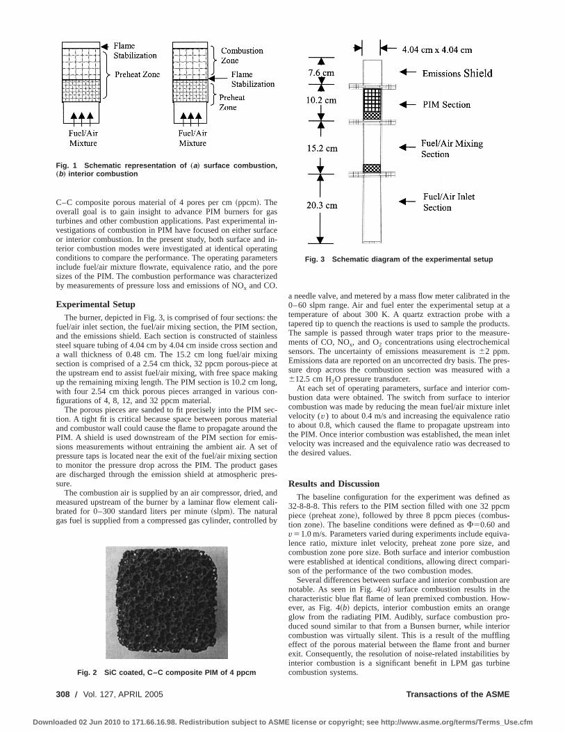
C–C composite porous material of 4 pores per cm~ppcm!. Theoverall goal is to gain insight to advance PIM burners for gasturbines and other combustion applications. Past experimental in-vestigations of combustion in PIM have focused on either surfaceor interior combustion. In the present study, both surface and in-terior combustion modes were investigated at identical operatingconditions to compare the performance. The operating parametersinclude fuel/air mixture flowrate, equivalence ratio, and the poresizes of the PIM. The combustion performance was characterizedby measurements of pressure loss and emissions of NOx and CO.

Experimental SetupThe burner, depicted in Fig. 3, is comprised of four sections: the

fuel/air inlet section, the fuel/air mixing section, the PIM section,and the emissions shield. Each section is constructed of stainlesssteel square tubing of 4.04 cm by 4.04 cm inside cross section anda wall thickness of 0.48 cm. The 15.2 cm long fuel/air mixingsection is comprised of a 2.54 cm thick, 32 ppcm porous-piece atthe upstream end to assist fuel/air mixing, with free space makingup the remaining mixing length. The PIM section is 10.2 cm long,with four 2.54 cm thick porous pieces arranged in various con-figurations of 4, 8, 12, and 32 ppcm material.

The porous pieces are sanded to fit precisely into the PIM sec-tion. A tight fit is critical because space between porous materialand combustor wall could cause the flame to propagate around thePIM. A shield is used downstream of the PIM section for emis-sions measurements without entraining the ambient air. A set ofpressure taps is located near the exit of the fuel/air mixing sectionto monitor the pressure drop across the PIM. The product gasesare discharged through the emission shield at atmospheric pres-sure.

The combustion air is supplied by an air compressor, dried, andmeasured upstream of the burner by a laminar flow element cali-brated for 0–300 standard liters per minute~slpm!. The naturalgas fuel is supplied from a compressed gas cylinder, controlled by

a needle valve, and metered by a mass flow meter calibrated in the0–60 slpm range. Air and fuel enter the experimental setup at atemperature of about 300 K. A quartz extraction probe with atapered tip to quench the reactions is used to sample the products.The sample is passed through water traps prior to the measure-ments of CO, NOx, and O2 concentrations using electrochemicalsensors. The uncertainty of emissions measurement is62 ppm.Emissions data are reported on an uncorrected dry basis. The pres-sure drop across the combustion section was measured with a612.5 cm H2O pressure transducer.

At each set of operating parameters, surface and interior com-bustion data were obtained. The switch from surface to interiorcombustion was made by reducing the mean fuel/air mixture inletvelocity (v) to about 0.4 m/s and increasing the equivalence ratioto about 0.8, which caused the flame to propagate upstream intothe PIM. Once interior combustion was established, the mean inletvelocity was increased and the equivalence ratio was decreased tothe desired values.

Results and DiscussionThe baseline configuration for the experiment was defined as

32-8-8-8. This refers to the PIM section filled with one 32 ppcmpiece~preheat zone!, followed by three 8 ppcm pieces~combus-tion zone!. The baseline conditions were defined asF50.60 andv51.0 m/s. Parameters varied during experiments include equiva-lence ratio, mixture inlet velocity, preheat zone pore size, andcombustion zone pore size. Both surface and interior combustionwere established at identical conditions, allowing direct compari-son of the performance of the two combustion modes.

Several differences between surface and interior combustion arenotable. As seen in Fig. 4~a! surface combustion results in thecharacteristic blue flat flame of lean premixed combustion. How-ever, as Fig. 4~b! depicts, interior combustion emits an orangeglow from the radiating PIM. Audibly, surface combustion pro-duced sound similar to that from a Bunsen burner, while interiorcombustion was virtually silent. This is a result of the mufflingeffect of the porous material between the flame front and burnerexit. Consequently, the resolution of noise-related instabilities byinterior combustion is a significant benefit in LPM gas turbinecombustion systems.

Fig. 1 Schematic representation of „a… surface combustion,„b… interior combustion

Fig. 2 SiC coated, C–C composite PIM of 4 ppcm

Fig. 3 Schematic diagram of the experimental setup



Pressure DropPressure drop resulting from cold flow through the PIM ranged

from 0 to 1% of the operating pressure. Figure 5 presents thepercent pressure drop across various individual porous pieces~each 2.54 cm thick! and the baseline configuration~32-8-8-8! at arange of flow rates. As expected, the pressure drop increases withthe flowrate. Note that the measured pressure drop across the 32-8-8-8 configuration is within 5% of that calculated by adding thepressure drop across the individual pieces. Figure 6 presents per-cent pressure drop for surface and interior combustion over arange of flow rates. With surface combustion, the pressure drop inthe PIM is virtually the same as that for cold flow. Interior com-

bustion, however, more than doubles the pressure drop in the PIMsection, in part, because of the higher velocity of the productgasses moving through the PIM. Results suggest that pore sizeand thickness of the PIM region are important to minimize thepressure drop for practical applications.

CO and NOx EmissionsFirst, experiments were conducted to determine the uniformity

and length of the reaction zone. To quantify this, emissions pro-files at baseline conditions were~a! in the flow direction~vertical!along the combustor midpoint and~b! in the transverse~horizon-tal! direction at a vertical planez563 mm above the PIM surface.

Figure 7 presents data for NOx and CO emissions of surfaceand interior combustion versus vertical distance~z! above the PIMsurface. Both NOx and CO emissions of interior combustion areconstant throughout the entire length of the emissions shield.Therefore, all of the NOx and CO are generated within the PIM.However, surface combustion concentrations change radicallynear the PIM surface. CO concentration increases sharply as theemissions probe is lowered into the flame front. NOx concentra-tions decrease sharply as the probe is moved into the flame. Re-sults show that the NOx formation was completed withinz515 mm from the PIM surface. The CO oxidation however con-tinued downstream until aboutz535 mm.

Figure 8 presents NOx and CO concentrations of surface andinterior combustion versus horizontal distance~y! from the com-bustor midpoint atz563 mm. Evidently, the CO and NOx emis-sions are nearly constant over the entire width for the two com-bustion modes. Emissions profiles obtained with leaner mixturesshowed CO increasing and NOx decreasing near the combustorwall, which suggests a quenching effect of heat loss through thewall. Based on these results, the combustor midpoint atz563 mm was selected for all subsequent emissions measure-ments, representing the postreaction zone.

Effect of Reactant Flow Rate. Figures 9~a! and 10~a!present data for NOx emissions versus equivalence ratio at variousmean inlet velocities for surface and interior combustion, respec-tively. At a given equivalence ratio, the NOx concentration isweakly dependent on the mean inlet velocity, varying over a factorof 2. Khanna et al.@14# produced similar results, citing constantNOx emissions over a range of flame speeds or mixture flowrates.NOx increased exponentially with equivalence ratio, suggestingthermal mechanism as the primary source of NOx generation.Single digit NOx concentrations are obtained in both combustionmodes for equivalence ratios of up to 0.65. Figures 9~b! and 10~b!present CO concentrations for surface and interior combustion,respectively. Figure 9~b! shows that the CO concentration at agiven equivalence ratio is nearly independent of the flowrate forsurface combustion. Khanna et al.@14# observed similar results tothose depicted in Fig. 9~b!; little dependence of CO concentrationon reactant flow rate. The CO concentration increases withequivalence ratio, similar to the trend observed in nozzle-stabilized LPM flames@15#. Mital et al. @16# also observed in-creasing CO concentration with increasing equivalence ratio frominterior combustion using reticulated ceramics. Data presented atthe lowest equivalence ratio in Figs. 9 and 10 correspond to thelean blow-off limit. Results show that the equivalence ratio at thelean blow-off limit increases with increasing mean inlet velocity.

In general, the CO concentration for interior combustion in-creases with equivalence ratio as shown in Fig. 10~b!. In this case,a significant flowrate effect is observed, especially at lower flow-rates. Note that the combustor was air-cooled by natural convec-tion to prevent overheating and structural damage to the stainlesssteel enclosure. At low flowrates, a larger fraction of heat releasedis believed to be lost to the surroundings. The resulting decreasein the flame temperature could affect the oxidation reactions toproduce larger CO concentrations. The fractional heat loss is ex-pected to diminish at higher flow rates, which show minor effecton CO emissions.

Fig. 4 Visual images at baseline conditions „a… surface com-bustion, „b… interior combustion

Fig. 5 Effect of pore size on cold flow pressure drop

Fig. 6 Effect of combustion on pressure drop for baselineconfiguration „32-8-8-8…, FÄ0.6



Surface Versus Interior Combustion. NOx and CO concen-trations versus equivalence ratio for surface and interior combus-tion at various flow rates are compared in Fig. 11 forv51.0 m/s. Results show that the combustion mode has little im-pact on NOx concentration at a given equivalence ratio. Interiorcombustion extends the lean blow-off limit, offering further NOxreduction. At the baseline conditions, the lean blow-off limit forsurface combustion is about 0.58 while that for interior combus-tion is 0.55. Theoretically, this extension of the lean blow-off limitcorresponds to a decrease in flame temperature of about 50 K. COconcentrations of the two combustion modes follow a similar

trend with equivalence ratio, although interior combustion resultsin slightly higher concentrations, attributed to a higher fractionheat loss as explained above.

Effect of Combustion Zone Pore Size. Thermal feedback toreactants in both combustion modes depends upon the geometryof the PIM. To examine this issue, surface combustion experi-ments were conducted with 4, 8, 12, and 32 ppcm PIM and inte-rior combustion experiments were conducted only with 4 and 8ppcm PIM because smaller pores would quench the flame. Resultsin Figs. 12~a! and 13~a! show a relatively weak trend of larger

Fig. 7 Effect of vertical measurement location on emissions „a… NOx and „b… CO

Fig. 8 Effect of horizontal measurement location on emissions „a… NOx and „b… CO

Fig. 9 Effects of mean inlet velocity on emissions from surface combustion, „a… NOx and „b… CO



pores resulting in higher NOx emissions at a given equivalenceratio. The PIM with larger pores has smaller optical thicknesscompared to that of a PIM with smaller pores. Therefore, it isplausible that the higher NOx generation of the large pore PIM~32-4-4-4! is an effect of the greater preheating of reactants byradiation from the flame zone. Detailed measurements near theflame front are therefore necessary to fully explain these observa-tions.

Figures 12~b! and 13~b! present CO concentration versusequivalence ratio for various combustion zone pore sizes, respec-

tively, for surface and interior combustion. In both cases, CO con-centration increases with decreasing pore size. Several phenomenamay be responsible for this trend. In case of surface combustion,increased flame length and residence time with larger pores wouldassist oxidation reactions to reduce CO emissions. Furthermore, asdiscussed above, a porous structure with smaller pores has a largeroptical thickness than a similar porous structure with larger pores.Therefore, less heat is radiated upstream and less preheating ofreactants occurs. The decrease in preheating is akin to the flame

Fig. 10 Effects of mean inlet velocity on emissions from interior combustion, „a… NOx and „b… CO

Fig. 11 Emissions measurements for the two combustion modes, „a… NOx and „b… CO

Fig. 12 Effect of combustion zone pore size on emission from surface combustion at vÄ1.0 mÕs, „a… NOx and „b…CO



leading to higher CO emissions. Flow dynamics on the pore sizescale level is another factor affecting CO concentration. Smallpores cause greater redirection of the gases moving through thestructures, resulting in increased local velocities. The increasedvelocity results in a higher strain rate for small pore size struc-tures, leading to higher CO concentrations at a given equivalenceratio.

Preheat Zone Pore Size. The degree of reactant preheatingfor interior combustion is largely dependent upon pore size of thepreheat zone. The size of the pores in this region must be small toenough to quench the flame and eliminate flashback. However, thepores should be large enough to allow significant thermal feed-back to the reactants. The effect of upstream pore size on emis-sions for interior combustion is presented in Fig. 14. At a givenequivalence ratio, NOx concentrations for the two preheat zonepore sizes tested were virtually identical. Figure 14~b! shows anoticeable reduction in CO concentration with larger preheat zonepore size, suggesting more effective preheating of reactants. Ex-tension of the lean blow-off limit with large pore size furthersubstantiates this observation. No flashback occurred at any of theconditions with the 32 ppcm preheat region. However, flashbackoccurred with the 12 ppcm preheat region at equivalence ratiosabove 0.58 and mean inlet velocity of 1.0 m/s. This result indi-cates that the preheat region pore size should be optimized toincrease the heat transfer upstream and to quench the reaction atthe most likely flashback conditions.

Concluding Remarks

SiC coated, C–C composite foam structures, offering superiorstructural and thermal integrity at gas turbine operating condi-tions, were investigated as PIM for combustion. Methane/airflames were stabilized on the surface and interior of the PIM atidentical operating conditions, allowing for a direct comparison ofthe two combustion modes. Simultaneous NOx and CO emissionsof less than 10 ppm were obtained for a range of equivalenceratios and mean inlet flowrates. While surface combustion pro-duced noise typical of a flat flame burner, interior combustion wasvirtually silent. The main results of this study are summarized inthe following:

~1! Surface combustion resulted in only slight increase in pres-sure drop in the PIM compared to that in cold flow. How-ever, interior combustion increases the pressure drop bymore than a factor of 2.

~2! For both combustion modes, the NOx concentration wasweakly dependent upon the flow velocity or PIM pore size.NOx concentration increased exponentially with equiva-lence ratio, suggesting thermal mechanism as the primarysource of NOx generation.

~3! For both combustion modes, the CO concentration in-creased with increasing equivalence ratio. The CO concen-tration decreased with increasing PIM pore size.

Fig. 13 Effect of combustion zone pore size on emission from interior combustion at vÄ1.0 mÕs, „a… NOx and „b… CO

Fig. 14 Effect of preheat zone pore size on emissions from interior combustion at vÄ1.0 mÕs, „a… NOx and „b… CO



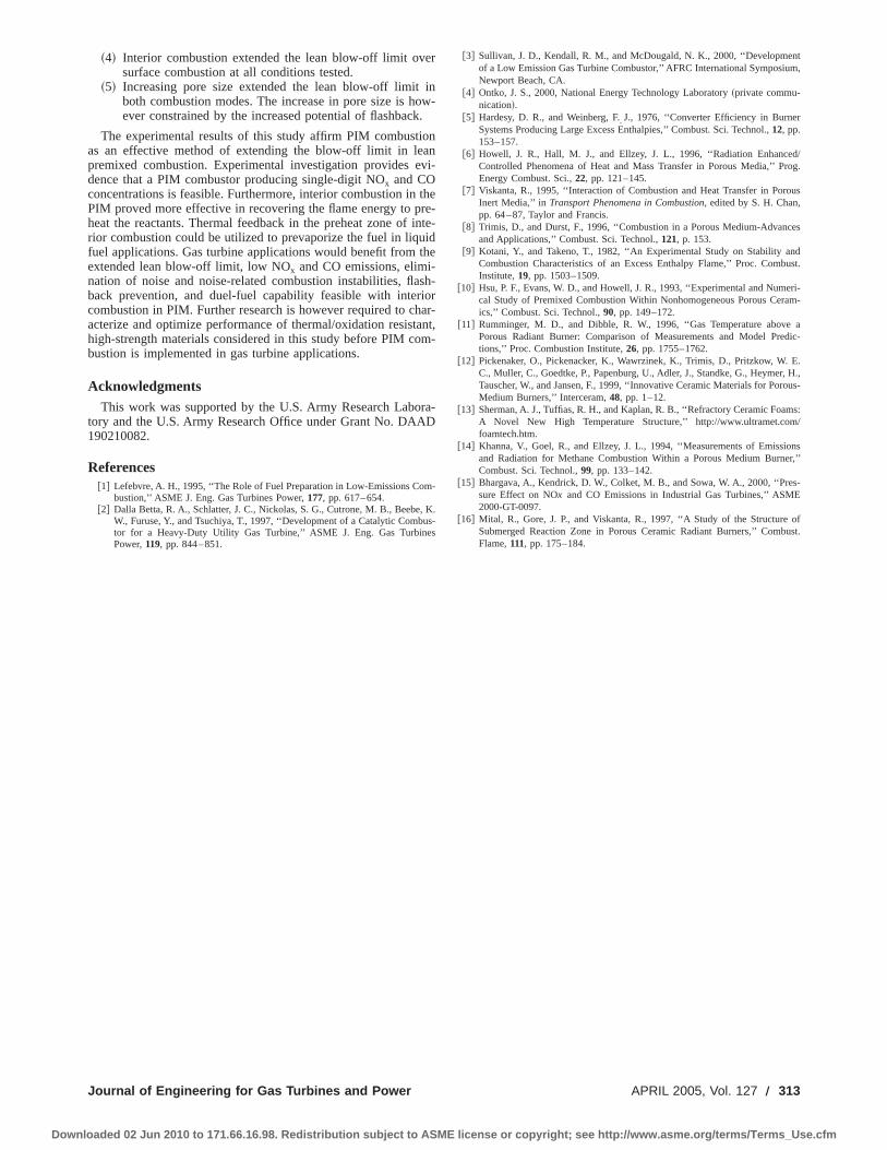
~4! Interior combustion extended the lean blow-off limit oversurface combustion at all conditions tested.

~5! Increasing pore size extended the lean blow-off limit inboth combustion modes. The increase in pore size is how-ever constrained by the increased potential of flashback.

The experimental results of this study affirm PIM combustionas an effective method of extending the blow-off limit in leanpremixed combustion. Experimental investigation provides evi-dence that a PIM combustor producing single-digit NOx and COconcentrations is feasible. Furthermore, interior combustion in thePIM proved more effective in recovering the flame energy to pre-heat the reactants. Thermal feedback in the preheat zone of inte-rior combustion could be utilized to prevaporize the fuel in liquidfuel applications. Gas turbine applications would benefit from theextended lean blow-off limit, low NOx and CO emissions, elimi-nation of noise and noise-related combustion instabilities, flash-back prevention, and duel-fuel capability feasible with interiorcombustion in PIM. Further research is however required to char-acterize and optimize performance of thermal/oxidation resistant,high-strength materials considered in this study before PIM com-bustion is implemented in gas turbine applications.

AcknowledgmentsThis work was supported by the U.S. Army Research Labora-

tory and the U.S. Army Research Office under Grant No. DAAD190210082.

References@1# Lefebvre, A. H., 1995, ‘‘The Role of Fuel Preparation in Low-Emissions Com-

bustion,’’ ASME J. Eng. Gas Turbines Power,177, pp. 617–654.@2# Dalla Betta, R. A., Schlatter, J. C., Nickolas, S. G., Cutrone, M. B., Beebe, K.

W., Furuse, Y., and Tsuchiya, T., 1997, ‘‘Development of a Catalytic Combus-tor for a Heavy-Duty Utility Gas Turbine,’’ ASME J. Eng. Gas TurbinesPower,119, pp. 844–851.

@3# Sullivan, J. D., Kendall, R. M., and McDougald, N. K., 2000, ‘‘Developmentof a Low Emission Gas Turbine Combustor,’’AFRC International Symposium,Newport Beach, CA.

@4# Ontko, J. S., 2000, National Energy Technology Laboratory~private commu-nication!.

@5# Hardesy, D. R., and Weinberg, F. J., 1976, ‘‘Converter Efficiency in BurnerSystems Producing Large Excess E˙nthalpies,’’ Combust. Sci. Technol.,12, pp.153–157.

@6# Howell, J. R., Hall, M. J., and Ellzey, J. L., 1996, ‘‘Radiation Enhanced/Controlled Phenomena of Heat and Mass Transfer in Porous Media,’’ Prog.Energy Combust. Sci.,22, pp. 121–145.

@7# Viskanta, R., 1995, ‘‘Interaction of Combustion and Heat Transfer in PorousInert Media,’’ in Transport Phenomena in Combustion, edited by S. H. Chan,pp. 64–87, Taylor and Francis.

@8# Trimis, D., and Durst, F., 1996, ‘‘Combustion in a Porous Medium-Advancesand Applications,’’ Combust. Sci. Technol.,121, p. 153.

@9# Kotani, Y., and Takeno, T., 1982, ‘‘An Experimental Study on Stability andCombustion Characteristics of an Excess Enthalpy Flame,’’ Proc. Combust.Institute,19, pp. 1503–1509.

@10# Hsu, P. F., Evans, W. D., and Howell, J. R., 1993, ‘‘Experimental and Numeri-cal Study of Premixed Combustion Within Nonhomogeneous Porous Ceram-ics,’’ Combust. Sci. Technol.,90, pp. 149–172.

@11# Rumminger, M. D., and Dibble, R. W., 1996, ‘‘Gas Temperature above aPorous Radiant Burner: Comparison of Measurements and Model Predic-tions,’’ Proc. Combustion Institute,26, pp. 1755–1762.

@12# Pickenaker, O., Pickenacker, K., Wawrzinek, K., Trimis, D., Pritzkow, W. E.C., Muller, C., Goedtke, P., Papenburg, U., Adler, J., Standke, G., Heymer, H.,Tauscher, W., and Jansen, F., 1999, ‘‘Innovative Ceramic Materials for Porous-Medium Burners,’’ Interceram,48, pp. 1–12.

@13# Sherman, A. J., Tuffias, R. H., and Kaplan, R. B., ‘‘Refractory Ceramic Foams:A Novel New High Temperature Structure,’’ http://www.ultramet.com/foamtech.htm.

@14# Khanna, V., Goel, R., and Ellzey, J. L., 1994, ‘‘Measurements of Emissionsand Radiation for Methane Combustion Within a Porous Medium Burner,’’Combust. Sci. Technol.,99, pp. 133–142.

@15# Bhargava, A., Kendrick, D. W., Colket, M. B., and Sowa, W. A., 2000, ‘‘Pres-sure Effect on NOx and CO Emissions in Industrial Gas Turbines,’’ ASME2000-GT-0097.

@16# Mital, R., Gore, J. P., and Viskanta, R., 1997, ‘‘A Study of the Structure ofSubmerged Reaction Zone in Porous Ceramic Radiant Burners,’’ Combust.Flame,111, pp. 175–184.



Meng Hee LimResearch Officer


M. Salman LeongProfessor


Institute of Noise and Vibration,University of Technology,

54100 Kuala Lumpur,Malaysia

Diagnosis for Loose Blades inGas Turbines Using WaveletAnalysisThe application of wavelet analysis to diagnose loose blades condition in gas turbines isexamined in this paper. Experimental studies were undertaken to simulate loose bladescondition occurring in gas turbines in an attempt to understand vibration response asso-ciated with loose blades under different operating conditions. Results showed that looseblades were undetectable under steady state operating condition. During turbine coastdown, a loose blade could be detected based on the impactic signals induced by the looseblades on the rotor and thus excited the natural frequencies of the rotor assembly. Resultsfrom the coast down condition showed that wavelet analysis was more sensitive andeffective than Fourier analysis for loose blade diagnosis. The severity, the number, andthe configuration of the loose blades could be potentially estimated based on the patternof the coast down wavelet map.@DOI: 10.1115/1.1772406#

1 Introduction

Blade faults represent a major and common source of problemin power generation gas turbines. Over the years, extensive re-search had been undertaken on this subject. Previous work re-ported in the literature included studies on the characteristics ofvarious blade faults and potential diagnostic methods. Reviews onthis subject were published by Meher-Homji@1–4# among others.The reviews showed emphasis on blade faults involving bladerubs, blade cracks, foreign object damage~FOD! or loss part,blade deformation~creeping and bending!, blade fouling, blademistuning, and blade fatigue failure. To the author’s knowledge, itwas Kuo @5# who attempted to address the problem of looseblades in gas turbine. Dynamic response and characteristics ofloose blades in gas turbines are therefore less quantified. Thereappeared to be limited effective diagnostic method in the detectionof loose blades in gas turbine. When loose blade is suspected ingas turbines, the methods used usually involved methods moresuitable for conventional faults. These include blade passing fre-quencies~BPF! monitoring ~suitable for blade rubbing!, perfor-mance monitoring method~suitable for blade fouling!, and pres-sure measurement method~suitable for blade deformation!. Suchmethods are often exclusively suitable for a specific blade faultonly and are less effective or sensitive in detecting other bladefaults. It is therefore very unlikely to find a unifying methodwhich is well suited to diagnose all kinds of blade faults that couldpossibly occur in gas turbines. Furthermore, these methods areusually based on the measurement~either vibration, pressure,noise, etc.! taken during the steady-state operating conditions. It isalso often the case that changes~in vibration, pressure or noise!resulting from a defect or fault may not appear in all operatingspeeds ranges. It was intention of this work to examine vibrationresponse of loose blade under different operating conditions~steady-state operating condition and coast down condition!, andto formulate suitable diagnostic methods from this experimentalstudy. In this paper, the potential of the wavelet analysis methodto be used for diagnosis of loose blades was examined and com-pared against conventional Fourier analysis method.

2 Experience of a Loose Blade ProblemLoose blades, and more pertinently intermediate packing pieces

which are used as spaces in securing individual blades, had beenknown to occur in some commercial gas turbines~for example,ABB gas turbines,@6#!. The experience of the authors related tofour-unit commercial open cycle gas turbines used in power gen-eration. The axial flow compressor section of the gas turbine had21 blading stages. The compressor stator and rotor blades weremade of high-tensile ferrite chrome steel, and manufactured partlyby precision forging and part milling. The blades were fitted intothe radial grooves of the rotor and compressor casing and wereseparated by the intermediate pieces~Fig. 1!. Rotor blades of thefirst ten stages were fitted directly in the rotor shaft by fir treeroots, while the blades for the remaining stages are rooted in theintermediate pieces. It was at these latter stages that the problemof loose blade problem was more prevalent due to the root orattachment design of the intermediate pieces.

From previous inspections on the turbines, visual observationsshowed that some intermediate pieces, particularly from stages 11to 21 protruded out and/or had cracks at the roots~see Fig. 2!.This fault could potentially result in further secondary failures,particularly foreign object damage~FOD!, if the roots of the in-termediate pieces completely failed. In addition to the crackedroot~s!, blades in the vicinity were also found loose. Copper rings~Fig. 1! used in the assembly beneath the loose blade were foundflattened; hence providing the room for the blades to loosen. Thissuggested that the root cause of the cracks on intermediate piecescould originate from the loose blades at this particular location. Itwas likely that the space provided by the flattened ring and rotorgrooves enabled the loose blade to rattle~vibrate!, with similarrattling of the intermediate pieces. Cracks eventually developed atthe roots of the intermediate pieces.

Some power plant operators in the Asia Pacific region are in-creasingly faced with the dilemma to operate their gas turbinesbeyond recommended running hours~EOH! stipulated by themanufacturers due to continuous electricity load demand and eco-nomic pressure for plant availability~Ng and Zahir@6#!. The de-mands in pressing electricity load despatch appeared to be a com-mon occurrence in the power generation industry world wide.Manufacturers~OEM! recommend preventive maintenance, in-cluding blades replacement, on the basis that life expectancy ofcomponents is reached upon specific running hours. The necessityand experience of the Connaught Bridge Power Station~CBPS! ofa public utility company in Malaysia, and the experience of the




authors in assisting the Station in seeking out feasible vibrationmonitoring and assessment for blades looseness and cracks onthese actual gas turbines, lead to experimental studies to be un-dertaken in the laboratory.

3 Experiment Test RigA test rig consisting of sub-assemblies of rotor-shaft, blades and

intermediate locking pieces, drive and casing was designed for alaboratory study of typical loose blade dynamic response. A hol-low rotor of 300 mm nominal diameter was used on the basis of apractical working dimension~and machining constraints!. Bladeswere located onto radial grooves in similar manner to the aboveindustrial gas turbines, although simplified for the purpose of thisexperimental study. Flat blades were used to avoid undue compli-cations in attempting to replicate the aerodynamic profile of anactual blade. Other basic features such as blade incidence angle,width, length and thickness were nevertheless maintained. Thetest rotor had 12 blades. A photograph showing an overall view isgiven in Fig. 3, and the blade assembly is given in Fig. 4. The testrig incorporated elements which were considered important forunderstanding the behavior of loose blade. A slackness adjusterand locking mechanism was incorporated into each blade suchthat controlled looseness could be induced in each blade.

Experiments were undertaken to quantify a tight and inducedfault condition. Three different conditions were incorporated in

this study. The first condition was such that only a single looseblade~abbreviated as ‘‘S’’! was introduced into the test rig. Thiscondition was designed to examine whether if the effect of a looseblade could be differentiated in the vibration spectrum of the rotorbearing measured under rotation. Fourier analysis and waveletanalysis were undertaken to confirm its viability and sensitivity todetect the loose blade. The second loose blade condition was in-duced such that all implanted loose blades were seated in adjacent

Fig. 1 Basic configuration of compressor rotor and its pertinent components„Ng and Zahir †6‡…

Fig. 2 Typical crack location on intermediate pieces „Ng andZahir †6‡…

Fig. 3 View of the experimental test rig

Fig. 4 Photograph showing blade assembly with intermediatelocking pieces



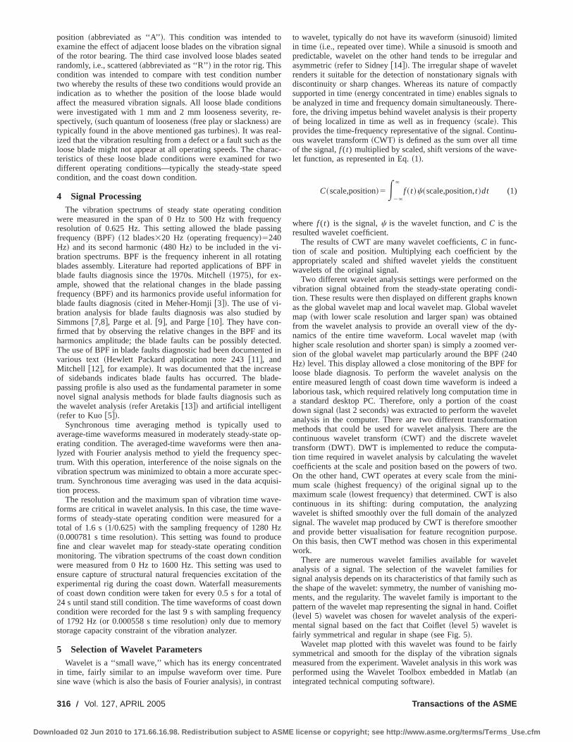
position ~abbreviated as ‘‘A’’!. This condition was intended toexamine the effect of adjacent loose blades on the vibration signalof the rotor bearing. The third case involved loose blades seatedrandomly, i.e., scattered~abbreviated as ‘‘R’’! in the rotor rig. Thiscondition was intended to compare with test condition numbertwo whereby the results of these two conditions would provide anindication as to whether the position of the loose blade wouldaffect the measured vibration signals. All loose blade conditionswere investigated with 1 mm and 2 mm looseness severity, re-spectively,~such quantum of looseness~free play or slackness! aretypically found in the above mentioned gas turbines!. It was real-ized that the vibration resulting from a defect or a fault such as theloose blade might not appear at all operating speeds. The charac-teristics of these loose blade conditions were examined for twodifferent operating conditions—typically the steady-state speedcondition, and the coast down condition.

4 Signal ProcessingThe vibration spectrums of steady state operating condition

were measured in the span of 0 Hz to 500 Hz with frequencyresolution of 0.625 Hz. This setting allowed the blade passingfrequency~BPF! ~12 blades320 Hz ~operating frequency!5240Hz! and its second harmonic~480 Hz! to be included in the vi-bration spectrums. BPF is the frequency inherent in all rotatingblades assembly. Literature had reported applications of BPF inblade faults diagnosis since the 1970s. Mitchell~1975!, for ex-ample, showed that the relational changes in the blade passingfrequency~BPF! and its harmonics provide useful information forblade faults diagnosis~cited in Meher-Homji@3#!. The use of vi-bration analysis for blade faults diagnosis was also studied bySimmons@7,8#, Parge et al.@9#, and Parge@10#. They have con-firmed that by observing the relative changes in the BPF and itsharmonics amplitude; the blade faults can be possibly detected.The use of BPF in blade faults diagnostic had been documented invarious text ~Hewlett Packard application note 243@11#, andMitchell @12#, for example!. It was documented that the increaseof sidebands indicates blade faults has occurred. The blade-passing profile is also used as the fundamental parameter in somenovel signal analysis methods for blade faults diagnosis such asthe wavelet analysis~refer Aretakis@13#! and artificial intelligent~refer to Kuo@5#!.

Synchronous time averaging method is typically used toaverage-time waveforms measured in moderately steady-state op-erating condition. The averaged-time waveforms were then ana-lyzed with Fourier analysis method to yield the frequency spec-trum. With this operation, interference of the noise signals on thevibration spectrum was minimized to obtain a more accurate spec-trum. Synchronous time averaging was used in the data acquisi-tion process.

The resolution and the maximum span of vibration time wave-forms are critical in wavelet analysis. In this case, the time wave-forms of steady-state operating condition were measured for atotal of 1.6 s~1/0.625! with the sampling frequency of 1280 Hz~0.000781 s time resolution!. This setting was found to producefine and clear wavelet map for steady-state operating conditionmonitoring. The vibration spectrums of the coast down conditionwere measured from 0 Hz to 1600 Hz. This setting was used toensure capture of structural natural frequencies excitation of theexperimental rig during the coast down. Waterfall measurementsof coast down condition were taken for every 0.5 s for a total of24 s until stand still condition. The time waveforms of coast downcondition were recorded for the last 9 s with sampling frequencyof 1792 Hz~or 0.000558 s time resolution! only due to memorystorage capacity constraint of the vibration analyzer.

5 Selection of Wavelet ParametersWavelet is a ‘‘small wave,’’ which has its energy concentrated

in time, fairly similar to an impulse waveform over time. Puresine wave~which is also the basis of Fourier analysis!, in contrast

to wavelet, typically do not have its waveform~sinusoid! limitedin time ~i.e., repeated over time!. While a sinusoid is smooth andpredictable, wavelet on the other hand tends to be irregular andasymmetric~refer to Sidney@14#!. The irregular shape of waveletrenders it suitable for the detection of nonstationary signals withdiscontinuity or sharp changes. Whereas its nature of compactlysupported in time~energy concentrated in time! enables signals tobe analyzed in time and frequency domain simultaneously. There-fore, the driving impetus behind wavelet analysis is their propertyof being localized in time as well as in frequency~scale!. Thisprovides the time-frequency representative of the signal. Continu-ous wavelet transform~CWT! is defined as the sum over all timeof the signal,f (t) multiplied by scaled, shift versions of the wave-let function, as represented in Eq.~1!.

C~scale,position!5E2`

`

f ~ t !c~scale,position,t !dt (1)

where f (t) is the signal,c is the wavelet function, andC is theresulted wavelet coefficient.

The results of CWT are many wavelet coefficients,C in func-tion of scale and position. Multiplying each coefficient by theappropriately scaled and shifted wavelet yields the constituentwavelets of the original signal.

Two different wavelet analysis settings were performed on thevibration signal obtained from the steady-state operating condi-tion. These results were then displayed on different graphs knownas the global wavelet map and local wavelet map. Global waveletmap ~with lower scale resolution and larger span! was obtainedfrom the wavelet analysis to provide an overall view of the dy-namics of the entire time waveform. Local wavelet map~withhigher scale resolution and shorter span! is simply a zoomed ver-sion of the global wavelet map particularly around the BPF~240Hz! level. This display allowed a close monitoring of the BPF forloose blade diagnosis. To perform the wavelet analysis on theentire measured length of coast down time waveform is indeed alaborious task, which required relatively long computation time ina standard desktop PC. Therefore, only a portion of the coastdown signal~last 2 seconds! was extracted to perform the waveletanalysis in the computer. There are two different transformationmethods that could be used for wavelet analysis. There are thecontinuous wavelet transform~CWT! and the discrete wavelettransform~DWT!. DWT is implemented to reduce the computa-tion time required in wavelet analysis by calculating the waveletcoefficients at the scale and position based on the powers of two.On the other hand, CWT operates at every scale from the mini-mum scale~highest frequency! of the original signal up to themaximum scale~lowest frequency! that determined. CWT is alsocontinuous in its shifting: during computation, the analyzingwavelet is shifted smoothly over the full domain of the analyzedsignal. The wavelet map produced by CWT is therefore smootherand provide better visualisation for feature recognition purpose.On this basis, then CWT method was chosen in this experimentalwork.

There are numerous wavelet families available for waveletanalysis of a signal. The selection of the wavelet families forsignal analysis depends on its characteristics of that family such asthe shape of the wavelet: symmetry, the number of vanishing mo-ments, and the regularity. The wavelet family is important to thepattern of the wavelet map representing the signal in hand. Coiflet~level 5! wavelet was chosen for wavelet analysis of the experi-mental signal based on the fact that Coiflet~level 5! wavelet isfairly symmetrical and regular in shape~see Fig. 5!.

Wavelet map plotted with this wavelet was found to be fairlysymmetrical and smooth for the display of the vibration signalsmeasured from the experiment. Wavelet analysis in this work wasperformed using the Wavelet Toolbox embedded in Matlab~anintegrated technical computing software!.



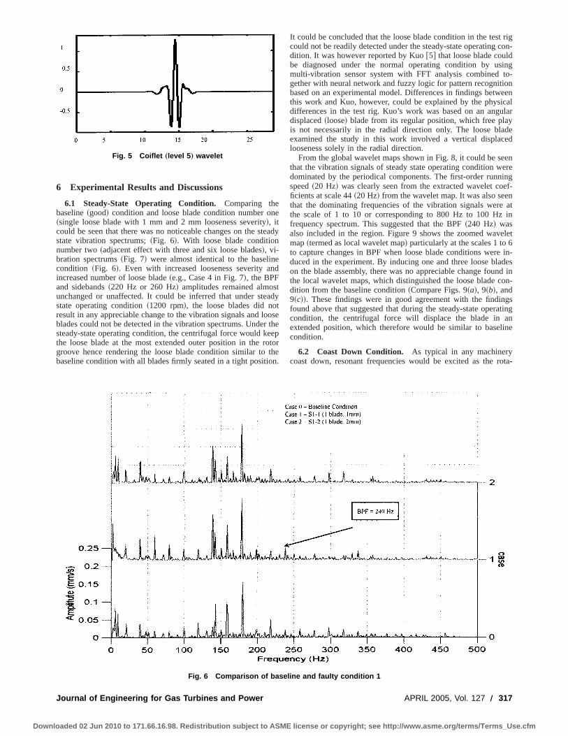
6 Experimental Results and Discussions

6.1 Steady-State Operating Condition. Comparing thebaseline~good! condition and loose blade condition number one~single loose blade with 1 mm and 2 mm looseness severity!, itcould be seen that there was no noticeable changes on the steadystate vibration spectrums;~Fig. 6!. With loose blade conditionnumber two~adjacent effect with three and six loose blades!, vi-bration spectrums~Fig. 7! were almost identical to the baselinecondition ~Fig. 6!. Even with increased looseness severity andincreased number of loose blade~e.g., Case 4 in Fig. 7!, the BPFand sidebands~220 Hz or 260 Hz! amplitudes remained almostunchanged or unaffected. It could be inferred that under steadystate operating condition~1200 rpm!, the loose blades did notresult in any appreciable change to the vibration signals and looseblades could not be detected in the vibration spectrums. Under thesteady-state operating condition, the centrifugal force would keepthe loose blade at the most extended outer position in the rotorgroove hence rendering the loose blade condition similar to thebaseline condition with all blades firmly seated in a tight position.

It could be concluded that the loose blade condition in the test rigcould not be readily detected under the steady-state operating con-dition. It was however reported by Kuo@5# that loose blade couldbe diagnosed under the normal operating condition by usingmulti-vibration sensor system with FFT analysis combined to-gether with neural network and fuzzy logic for pattern recognitionbased on an experimental model. Differences in findings betweenthis work and Kuo, however, could be explained by the physicaldifferences in the test rig. Kuo’s work was based on an angulardisplaced~loose! blade from its regular position, which free playis not necessarily in the radial direction only. The loose bladeexamined the study in this work involved a vertical displacedlooseness solely in the radial direction.

From the global wavelet maps shown in Fig. 8, it could be seenthat the vibration signals of steady state operating condition weredominated by the periodical components. The first-order runningspeed~20 Hz! was clearly seen from the extracted wavelet coef-ficients at scale 44~20 Hz! from the wavelet map. It was also seenthat the dominating frequencies of the vibration signals were atthe scale of 1 to 10 or corresponding to 800 Hz to 100 Hz infrequency spectrum. This suggested that the BPF~240 Hz! wasalso included in the region. Figure 9 shows the zoomed waveletmap~termed as local wavelet map! particularly at the scales 1 to 6to capture changes in BPF when loose blade conditions were in-duced in the experiment. By inducing one and three loose bladeson the blade assembly, there was no appreciable change found inthe local wavelet maps, which distinguished the loose blade con-dition from the baseline condition~Compare Figs. 9~a!, 9~b!, and9~c!!. These findings were in good agreement with the findingsfound above that suggested that during the steady-state operatingcondition, the centrifugal force will displace the blade in anextended position, which therefore would be similar to baselinecondition.

6.2 Coast Down Condition. As typical in any machinerycoast down, resonant frequencies would be excited as the rota-

Fig. 5 Coiflet „level 5 … wavelet

Fig. 6 Comparison of baseline and faulty condition 1



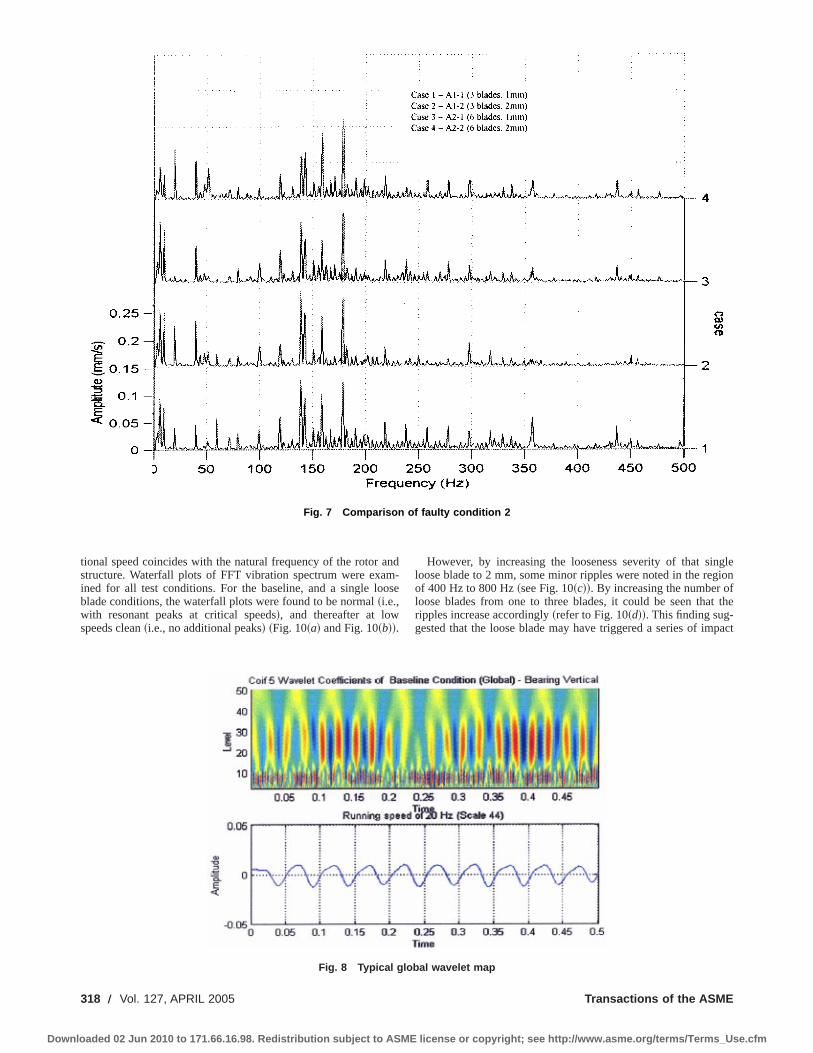
tional speed coincides with the natural frequency of the rotor andstructure. Waterfall plots of FFT vibration spectrum were exam-ined for all test conditions. For the baseline, and a single looseblade conditions, the waterfall plots were found to be normal~i.e.,with resonant peaks at critical speeds!, and thereafter at lowspeeds clean~i.e., no additional peaks! ~Fig. 10~a! and Fig. 10~b!!.

However, by increasing the looseness severity of that singleloose blade to 2 mm, some minor ripples were noted in the regionof 400 Hz to 800 Hz~see Fig. 10~c!!. By increasing the number ofloose blades from one to three blades, it could be seen that theripples increase accordingly~refer to Fig. 10~d!!. This finding sug-gested that the loose blade may have triggered a series of impact

Fig. 7 Comparison of faulty condition 2

Fig. 8 Typical global wavelet map



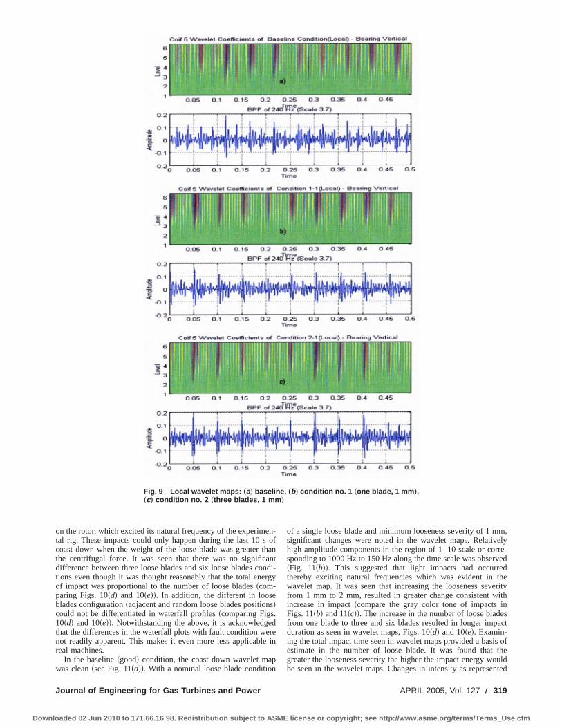
on the rotor, which excited its natural frequency of the experimen-tal rig. These impacts could only happen during the last 10 s ofcoast down when the weight of the loose blade was greater thanthe centrifugal force. It was seen that there was no significantdifference between three loose blades and six loose blades condi-tions even though it was thought reasonably that the total energyof impact was proportional to the number of loose blades~com-paring Figs. 10~d! and 10~e!!. In addition, the different in looseblades configuration~adjacent and random loose blades positions!could not be differentiated in waterfall profiles~comparing Figs.10~d! and 10~e!!. Notwithstanding the above, it is acknowledgedthat the differences in the waterfall plots with fault condition werenot readily apparent. This makes it even more less applicable inreal machines.

In the baseline~good! condition, the coast down wavelet mapwas clean~see Fig. 11~a!!. With a nominal loose blade condition

of a single loose blade and minimum looseness severity of 1 mm,significant changes were noted in the wavelet maps. Relativelyhigh amplitude components in the region of 1–10 scale or corre-sponding to 1000 Hz to 150 Hz along the time scale was observed~Fig. 11~b!!. This suggested that light impacts had occurredthereby exciting natural frequencies which was evident in thewavelet map. It was seen that increasing the looseness severityfrom 1 mm to 2 mm, resulted in greater change consistent withincrease in impact~compare the gray color tone of impacts inFigs. 11~b! and 11~c!!. The increase in the number of loose bladesfrom one blade to three and six blades resulted in longer impactduration as seen in wavelet maps, Figs. 10~d! and 10~e!. Examin-ing the total impact time seen in wavelet maps provided a basis ofestimate in the number of loose blade. It was found that thegreater the looseness severity the higher the impact energy wouldbe seen in the wavelet maps. Changes in intensity as represented

Fig. 9 Local wavelet maps: „a… baseline, „b… condition no. 1 „one blade, 1 mm …,„c… condition no. 2 „three blades, 1 mm …



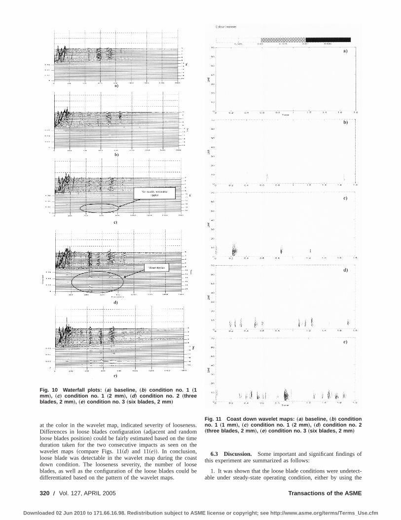
at the color in the wavelet map, indicated severity of looseness.Differences in loose blades configuration~adjacent and randomloose blades position! could be fairly estimated based on the timeduration taken for the two consecutive impacts as seen on thewavelet maps~compare Figs. 11~d! and 11~e!!. In conclusion,loose blade was detectable in the wavelet map during the coastdown condition. The looseness severity, the number of looseblades, as well as the configuration of the loose blades could bedifferentiated based on the pattern of the wavelet maps.

6.3 Discussion. Some important and significant findings ofthis experiment are summarized as follows:

1. It was shown that the loose blade conditions were undetect-able under steady-state operating condition, either by using the

Fig. 10 Waterfall plots: „a… baseline, „b… condition no. 1 „1mm …, „c… condition no. 1 „2 mm …, „d… condition no. 2 „threeblades, 2 mm …, „e… condition no. 3 „six blades, 2 mm …

Fig. 11 Coast down wavelet maps: „a… baseline, „b… conditionno. 1 „1 mm …, „c… condition no. 1 „2 mm …, „d… condition no. 2„three blades, 2 mm …, „e… condition no. 3 „six blades, 2 mm …



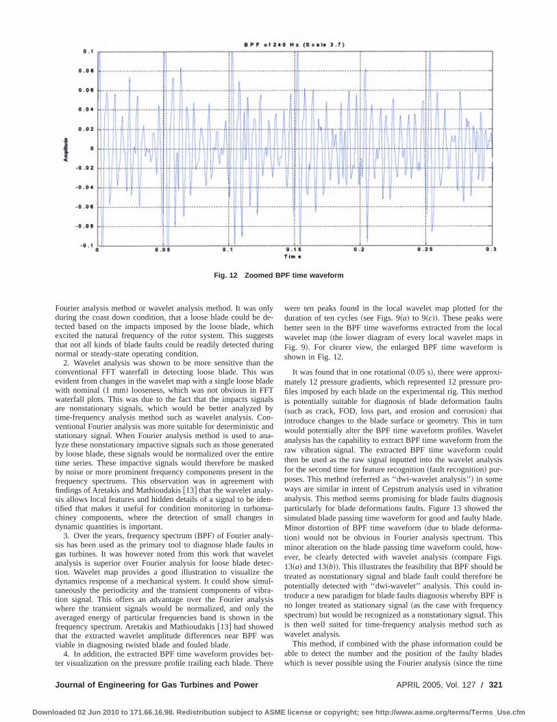
Fourier analysis method or wavelet analysis method. It was onlyduring the coast down condition, that a loose blade could be de-tected based on the impacts imposed by the loose blade, whichexcited the natural frequency of the rotor system. This suggeststhat not all kinds of blade faults could be readily detected duringnormal or steady-state operating condition.

2. Wavelet analysis was shown to be more sensitive than theconventional FFT waterfall in detecting loose blade. This wasevident from changes in the wavelet map with a single loose bladewith nominal ~1 mm! looseness, which was not obvious in FFTwaterfall plots. This was due to the fact that the impacts signalsare nonstationary signals, which would be better analyzed bytime-frequency analysis method such as wavelet analysis. Con-ventional Fourier analysis was more suitable for deterministic andstationary signal. When Fourier analysis method is used to ana-lyze these nonstationary impactive signals such as those generatedby loose blade, these signals would be normalized over the entiretime series. These impactive signals would therefore be maskedby noise or more prominent frequency components present in thefrequency spectrums. This observation was in agreement withfindings of Aretakis and Mathioudakis@13# that the wavelet analy-sis allows local features and hidden details of a signal to be iden-tified that makes it useful for condition monitoring in turboma-chiney components, where the detection of small changes indynamic quantities is important.

3. Over the years, frequency spectrum~BPF! of Fourier analy-sis has been used as the primary tool to diagnose blade faults ingas turbines. It was however noted from this work that waveletanalysis is superior over Fourier analysis for loose blade detec-tion. Wavelet map provides a good illustration to visualize thedynamics response of a mechanical system. It could show simul-taneously the periodicity and the transient components of vibra-tion signal. This offers an advantage over the Fourier analysiswhere the transient signals would be normalized, and only theaveraged energy of particular frequencies band is shown in thefrequency spectrum. Aretakis and Mathioudakis@13# had showedthat the extracted wavelet amplitude differences near BPF wasviable in diagnosing twisted blade and fouled blade.

4. In addition, the extracted BPF time waveform provides bet-ter visualization on the pressure profile trailing each blade. There

were ten peaks found in the local wavelet map plotted for theduration of ten cycles~see Figs. 9~a! to 9~c!!. These peaks werebetter seen in the BPF time waveforms extracted from the localwavelet map~the lower diagram of every local wavelet maps inFig. 9!. For clearer view, the enlarged BPF time waveform isshown in Fig. 12.

It was found that in one rotational~0.05 s!, there were approxi-mately 12 pressure gradients, which represented 12 pressure pro-files imposed by each blade on the experimental rig. This methodis potentially suitable for diagnosis of blade deformation faults~such as crack, FOD, loss part, and erosion and corrosion! thatintroduce changes to the blade surface or geometry. This in turnwould potentially alter the BPF time waveform profiles. Waveletanalysis has the capability to extract BPF time waveform from theraw vibration signal. The extracted BPF time waveform couldthen be used as the raw signal inputted into the wavelet analysisfor the second time for feature recognition~fault recognition! pur-poses. This method~referred as ‘‘dwi-wavelet analysis’’! in someways are similar in intent of Cepstrum analysis used in vibrationanalysis. This method seems promising for blade faults diagnosisparticularly for blade deformations faults. Figure 13 showed thesimulated blade passing time waveform for good and faulty blade.Minor distortion of BPF time waveform~due to blade deforma-tion! would not be obvious in Fourier analysis spectrum. Thisminor alteration on the blade passing time waveform could, how-ever, be clearly detected with wavelet analysis~compare Figs.13~a! and 13~b!!. This illustrates the feasibility that BPF should betreated as nonstationary signal and blade fault could therefore bepotentially detected with ‘‘dwi-wavelet’’ analysis. This could in-troduce a new paradigm for blade faults diagnosis whereby BPF isno longer treated as stationary signal~as the case with frequencyspectrum! but would be recognized as a nonstationary signal. Thisis then well suited for time-frequency analysis method such aswavelet analysis.

This method, if combined with the phase information could beable to detect the number and the position of the faulty bladeswhich is never possible using the Fourier analysis~since the time

Fig. 12 Zoomed BPF time waveform



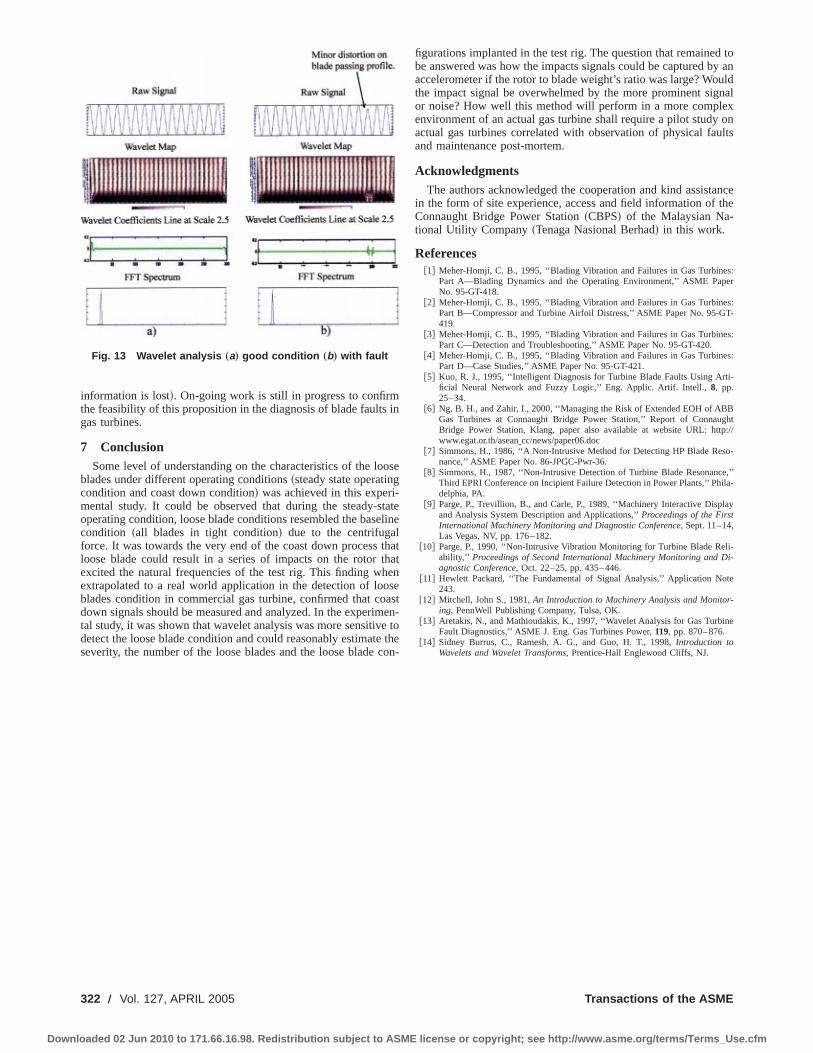
information is lost!. On-going work is still in progress to confirmthe feasibility of this proposition in the diagnosis of blade faults ingas turbines.

7 ConclusionSome level of understanding on the characteristics of the loose

blades under different operating conditions~steady state operatingcondition and coast down condition! was achieved in this experi-mental study. It could be observed that during the steady-stateoperating condition, loose blade conditions resembled the baselinecondition ~all blades in tight condition! due to the centrifugalforce. It was towards the very end of the coast down process thatloose blade could result in a series of impacts on the rotor thatexcited the natural frequencies of the test rig. This finding whenextrapolated to a real world application in the detection of looseblades condition in commercial gas turbine, confirmed that coastdown signals should be measured and analyzed. In the experimen-tal study, it was shown that wavelet analysis was more sensitive todetect the loose blade condition and could reasonably estimate theseverity, the number of the loose blades and the loose blade con-

figurations implanted in the test rig. The question that remained tobe answered was how the impacts signals could be captured by anaccelerometer if the rotor to blade weight’s ratio was large? Wouldthe impact signal be overwhelmed by the more prominent signalor noise? How well this method will perform in a more complexenvironment of an actual gas turbine shall require a pilot study onactual gas turbines correlated with observation of physical faultsand maintenance post-mortem.

AcknowledgmentsThe authors acknowledged the cooperation and kind assistance

in the form of site experience, access and field information of theConnaught Bridge Power Station~CBPS! of the Malaysian Na-tional Utility Company~Tenaga Nasional Berhad! in this work.

References@1# Meher-Homji, C. B., 1995, ‘‘Blading Vibration and Failures in Gas Turbines:

Part A—Blading Dynamics and the Operating Environment,’’ ASME PaperNo. 95-GT-418.

@2# Meher-Homji, C. B., 1995, ‘‘Blading Vibration and Failures in Gas Turbines:Part B—Compressor and Turbine Airfoil Distress,’’ ASME Paper No. 95-GT-419.

@3# Meher-Homji, C. B., 1995, ‘‘Blading Vibration and Failures in Gas Turbines:Part C—Detection and Troubleshooting,’’ ASME Paper No. 95-GT-420.

@4# Meher-Homji, C. B., 1995, ‘‘Blading Vibration and Failures in Gas Turbines:Part D—Case Studies,’’ ASME Paper No. 95-GT-421.

@5# Kuo, R. J., 1995, ‘‘Intelligent Diagnosis for Turbine Blade Faults Using Arti-ficial Neural Network and Fuzzy Logic,’’ Eng. Applic. Artif. Intell.,8, pp.25–34.

@6# Ng, B. H., and Zahir, I., 2000, ‘‘Managing the Risk of Extended EOH of ABBGas Turbines at Connaught Bridge Power Station,’’ Report of ConnaughtBridge Power Station, Klang, paper also available at website URL: http://www.egat.or.th/aseanIcc/news/paper06.doc

@7# Simmons, H., 1986, ‘‘A Non-Intrusive Method for Detecting HP Blade Reso-nance,’’ ASME Paper No. 86-JPGC-Pwr-36.

@8# Simmons, H., 1987, ‘‘Non-Intrusive Detection of Turbine Blade Resonance,’’Third EPRI Conference on Incipient Failure Detection in Power Plants,’’ Phila-delphia, PA.

@9# Parge, P., Trevillion, B., and Carle, P., 1989, ‘‘Machinery Interactive Displayand Analysis System Description and Applications,’’Proceedings of the FirstInternational Machinery Monitoring and Diagnostic Conference, Sept. 11–14,Las Vegas, NV, pp. 176–182.

@10# Parge, P., 1990, ‘‘Non-Intrusive Vibration Monitoring for Turbine Blade Reli-ability,’’ Proceedings of Second International Machinery Monitoring and Di-agnostic Conference, Oct. 22–25, pp. 435–446.

@11# Hewlett Packard, ‘‘The Fundamental of Signal Analysis,’’ Application Note243.

@12# Mitchell, John S., 1981,An Introduction to Machinery Analysis and Monitor-ing, PennWell Publishing Company, Tulsa, OK.

@13# Aretakis, N., and Mathioudakis, K., 1997, ‘‘Wavelet Analysis for Gas TurbineFault Diagnostics,’’ ASME J. Eng. Gas Turbines Power,119, pp. 870–876.

@14# Sidney Burrus, C., Ramesh, A. G., and Guo, H. T., 1998,Introduction toWavelets and Wavelet Transforms, Prentice-Hall Englewood Cliffs, NJ.

Fig. 13 Wavelet analysis „a… good condition „b… with fault



Dan SimonElectrical Engineering Department,

Cleveland State University,1960 East 24th Street,Cleveland, OH 44115


Donald L. SimonU.S. Army Research Laboratory,

NASA Glenn Research Center,21000 Brookpark Road,

Cleveland, OH 44138e-mail: [email protected]

Aircraft Turbofan Engine HealthEstimation Using ConstrainedKalman FilteringKalman filters are often used to estimate the state variables of a dynamic system. How-ever, in the application of Kalman filters some known signal information is often eitherignored or dealt with heuristically. For instance, state-variable constraints (which may bebased on physical considerations) are often neglected because they do not fit easily intothe structure of the Kalman filter. This paper develops an analytic method of incorporat-ing state-variable inequality constraints in the Kalman filter. The resultant filter is acombination of a standard Kalman filter and a quadratic programming problem. Theincorporation of state-variable constraints increases the computational effort of the filterbut significantly improves its estimation accuracy. The improvement is proven theoreti-cally and shown via simulation results obtained from application to a turbofan enginemodel. This model contains 16 state variables, 12 measurements, and 8 component healthparameters. It is shown that the new algorithms provide improved performance in thisexample over unconstrained Kalman filtering.@DOI: 10.1115/1.1789153#

IntroductionFor linear dynamic systems with white process and measure-

ment noise, the Kalman filter is known to be an optimal estimator.However, in the application of Kalman filters there is often knownmodel or signal information that is either ignored or dealt withheuristically@1#. This paper presents a way to generalize the Kal-man filter in such a way that known inequality constraints amongthe state variables are satisfied by the state-variable estimates.

The method presented here for enforcing inequality constraintson the state-variable estimates uses hard constraints. It is based ona generalization of the approach presented in Ref.@2#, which dealtwith the incorporation of state-variable equality constraints in theKalman filter. Inequality constraints are inherently more compli-cated than equality constraints, but standard quadratic program-ming results can be used to solve the Kalman-filter problem withinequality constraints. At each time step of the constrained Kal-man filter, we solve a quadratic programming problem to obtainthe constrained state estimate. A family of constrained state esti-mates is obtained, where the weighting matrix of the quadraticprogramming problem determines which family member formsthe desired solution. It is stated in this paper, on the basis of Ref.@2#, that the constrained estimate has several important properties.The constrained state estimate is unbiased~Theorem 1 below! andhas a smaller error covariance than the unconstrained estimate~Theorem 2 below!. We show which member of all possible con-strained solutions has the smallest error covariance~Theorem 3below!. We also show the one particular member that is always~i.e., at each time step! closer to the true state than the uncon-strained estimate~Theorem 4 below!. Finally, we show that thevariation of the constrained estimate is smaller than the variationof the unconstrained estimate~Theorem 5 below!.

The application considered in this paper is turbofan enginehealth-parameter estimation@3#. The performance of gas turbineengines deteriorates over time. This deterioration can affect thefuel economy and impact emissions, component life consumption,and thrust response of the engine. Airlines periodically collect

engine data in order to evaluate the health of the engine and itscomponents. The health evaluation is then used to determinemaintenance schedules. Reliable health evaluations are used toanticipate future maintenance needs. This offers the benefits ofimproved safety and reduced operating costs. The money-savingpotential of such health evaluations is substantial, but only if theevaluations are reliable. The data used to perform health evalua-tions are typically collected during flight and later transferred toground-based computers for post-flight analysis. Data are col-lected each flight at approximately the same engine operating con-ditions and corrected to account for variability in ambient condi-tions and power-setting levels. Typically, data are collected for aperiod of about 3 s at arate of about 10 or 20 Hz. Various algo-rithms have been proposed to estimate engine health parameters,such as weighted least squares@4#, expert systems@5#, Kalmanfilters @6#, neural networks@6#, and genetic algorithms@7#.

This paper applies constrained Kalman filtering to estimate en-gine component efficiencies and flow capacities, which are re-ferred to as health parameters. We can use our knowledge of thephysics of the turbofan engine in order to obtain a dynamic model@8,9#. The health parameters that we try to estimate can be mod-eled as slowly varying biases. The state vector of the dynamicmodel is augmented to include the health parameters, which arethen estimated with a Kalman filter@10#. The model formulationin this paper is similar to previous NASA work@11#. However,Ref. @11# was limited to a 3-state dynamic model and 2 healthparameters, whereas this present work includes a more complete16-state model and 8 health parameters. In addition, we havesome a priori knowledge of the engine’s health parameters: weknow that they never improve. Engine health always degradesover time, and we can incorporate this information into state con-straints to improve our health-parameter estimation.~This is as-suming that no maintenance or engine overhaul is performed.!This is similar to the probabilistic approach to turbofan prognos-tics proposed in Ref.@12#. The simulation results that we presenthere show that the Kalman filter can estimate health-parameterdeviations with an average error of less than 5%, and the con-strained Kalman filter performs even better than the unconstrainedfilter.

It should be emphasized that in this paper we are confining theproblem to the estimation of engine health parameters in the pres-ence of degradation only. There are specific engine fault scenariosthat can result in abrupt shifts in filter estimates, possibly even




indicating an apparent improvement in some engine components.An actual engine-performance monitoring system would need toinclude additional logic to detect and isolate such faults.

Kalman FilteringConsider the discrete linear time-invariant system given by

xk115Axk1Buk1wk ,(1)

yk5Cxk1ek ,

wherek is the time index,x is the state vector,u is the knowncontrol input,y is the measurement, and$wk% and$ek% are uncor-related zero-mean white-noise input sequences. We useQ to de-note the covariance of$wk% and R to denote the covariance of$ek%, and x to denote the expected value ofx. The problem is tofind an estimate xk11 of xk11 given the measurements$y0 ,y1 , . . . ,yk%. We will use the symbolYk to denote the columnvector that contains the measurements$y0 ,y1 , . . . ,yk%. The Kal-man filter can be used to solve this problem as follows:

Kk5ASkCT~CSkC

T1R!21, (2)

xk115Axk1Buk1Kk~yk2Cxk!, (3)

Sk115~ASk2KkCSk!AT1Q, (4)

where the filter is initialized withx05 x0 , and S05E@(x02 x0)3(x02 x0)T#. It can be shown@13# that the Kalman-filter estimatehas several attractive properties. It is unbiased, and of all affineestimators, it is the one that minimizes the variance of the estima-tion error. In addition, ifx0 , $wk%, and$ek% are jointly Gaussian,then the Kalman-filter estimate is the one that maximizes the con-ditional probability density function of the state given the mea-surement history.

Kalman Filtering With Inequality ConstraintsThis section extends the well-known results of the preceding

section to cases where there are known linear inequality con-straints among the state components. Also, several importantproperties of the constrained filter are discussed. Consider thedynamic system of Eq.~1! where we are given the additionalconstraint

Dxk<dk , (5)

where D is a knowns3n constant matrix,s is the number ofconstraints,n is the number of state variables, ands<n. It isassumed in this paper thatD is full rank, i.e., thatD has ranks.This is an easily satisfied assumption. IfD is not full rank thatmeans we have redundant state constraints. In that case we cansimply remove linearly dependent rows fromD ~i.e., remove re-dundant state constraints! until D is full rank. Three different ap-proaches to the constrained state estimation problem are given inthis section. The time indexk is omitted in the remainder of thissection for ease of notation.

The Maximum Probability Method. In this section we de-rive the constrained Kalman-filtering problem by using a maxi-mum probability method. From Ref.@@13#, p. 93ff.# we know thatthe Kalman-filter estimate is that value ofx that maximizes theconditional probability density functionP(xuY). The constrainedKalman filter can be derived by finding an estimatex such that theconditional probabilityP( xuY) is maximized andx satisfies theconstraint of Eq.~5!. Maximizing P( xuY) is the same as maxi-mizing its natural logarithm. So the problem we want to solve canbe given by

max lnP~ xuY!⇒minx

~ x2x% !TS21~ x2x% !,

(6)such thatDx<d.

Using the fact that the unconstrained state estimatex5x% ~the con-ditional mean ofx!, we rewrite the above equation as

minx

~ xTS21x22xTS21x!such thatDx<d. (7)

Note that this problem statement depends on the conditionalGaussian nature ofx, which in turn depends on the Gaussiannature ofx0 , $wk%, and$ek% in Eq. ~1!.

The Mean-Square Method. In this section we derive theconstrained Kalman-filtering problem by using a mean-squareminimization method. We seek to minimize the conditional mean-square error subject to the state constraints.

minx

E~ ix2 xi2uY!such thatDx<d, (8)

wherei•i denotes the vector two-norm. If we assume thatx andYare jointly Gaussian, the mean-square error can be written as

E~ ix2 xi2uY!5E ~x2 x!T~x2 x!P~xuY!dx (9)

5E xTxP~xuY!dx22xTE xP~xuY!dx1 xTx.

(10)

Noting that the Kalman-filter estimate is the conditional mean ofx, i.e.,

x5E xP~xuY!dx, (11)

we formulate the first-order conditions necessary for a minimumas

minx

~ xTx22xTx!such thatDx<d. (12)

Again, this problem statement depends on the conditional Gauss-ian nature ofx, which in turn depends on the Gaussian nature ofx0 , $wk%, and$ek% in Eq. ~1!.

The Projection Method. In this section we derive the con-strained Kalman-filtering problem by directly projecting the un-constrained state estimatex onto the constraint surface. That is,we solve the problem

minx

~ x2 x!TW~ x2 x!such thatDx<d, (13)

where W is any symmetric positive-definite weighting matrix.This problem can be rewritten as

minx

~ xTWx22xTWx!such thatDx<d. (14)

The constrained estimation problems derived by the maximumprobability method of Eq.~7! and the mean-square method of Eq.~12! can be obtained from this equation by settingW5S21 andW5I , respectively. Note that this derivation of the constrainedestimation problem does not depend on the conditional Gaussiannature ofx; i.e., x0 , $wk%, and$ek% in Eq. ~1! are not assumed tobe Gaussian.

The Solution of the Constrained-State Estimation Problem.The problem defined by Eq.~14! is known as a quadratic pro-gramming problem@14,15#. There are many algorithms for solv-ing quadratic programming problems, almost all of which fall inthe category known as active set methods. An active set methoduses the fact that it is only those constraints that are active at thesolution of the problem that are significant in the optimality con-ditions. Assume thatt of the s inequality constraints are active atthe solution of Eq.~14!, and denote byD and d the t rows of Dand t elements ofd corresponding to the active constraints. If the



correct set of active constraints was known a priori then the solu-tion of Eq. ~14! would also be a solution of the equality-constrained problem

minx

~ xTWx22xTWx!such that Dx5d. (15)

This shows that the inequality-constrained problem defined by Eq.~14! is equivalent to the equality-constrained problem defined byEq. ~15!. Note that x depends entirely onx at each time step.Although the equation forx is recursive as seen in Eq.~3!, theequation for x is not recursive. Therefore, an inequality-constrained Kalman filter that uses active set methods to enforcethe constraints completely reduces to an equality-constrained Kal-man filter, even though the active set may change at each timestep. The equality-constrained problem was discussed in Ref.@2#,in which there is no assumption that the constraints remain con-stant from one time step to the next. Therefore, those results canbe used to investigate the properties of the inequality-constrainedfilter.

Properties of the Constrained State Estimate. In this sec-tion we examine some of the statistical properties of the con-strained Kalman filter. We usex to denote the state estimate of theunconstrained Kalman filter, andx to denote the state estimate ofthe constrained Kalman filter as given by Eq.~14!, recalling thatEqs.~7! and ~12! are special cases of Eq.~14!.

Theorem 1. The solutionx of the constrained state estimationproblem given by Eq.~14! is an unbiased state estimator for thesystem given by Eq.~1! for any symmetric positive definiteweighting matrix W. That is,

E~ x!5E~x!. (16)

Theorem 2. The solutionx of the constrained state estimationproblem given by Eq.~14! with W5S21, whereS is the errorcovariance of the unconstrained estimate given in Eq.~4!, has anerror covariance that is less than or equal to that of the uncon-strained state estimate. That is,

Cov~x2 x!<Cov~x2 x!. (17)

At first this seems counterintuitive, since the standard Kalmanfilter is by definition the minimum variance filter. However, wehave changed the problem by introducing state-variable con-straints. Therefore, the standard Kalman filter is no longer theminimum variance filter, and we can do better with the con-strained Kalman filter.

Theorem 3. Among all the constrained Kalman filters result-ing from the solution of Eq.~14!, the filter that usesW5S21 hasthe smallest estimation error covariance. That is,

Cov~x2 xS21!<Cov~x2 xW! for all W. (18)

Theorem 4. The solutionx of the constrained state estimationproblem given by Eq.~14! with W5I satisfies the inequality

ixk2 xki<ixk2 xki for all k, (19)

where i•i is the vector two-norm andx is the unconstrainedKalman-filter estimate.

Theorem 5. The error of the solutionx of the constrained stateestimation problem given by Eq.~14! with W5I is smaller thanthe unconstrained estimation error in the sense that

Tr@Cov~ x!]<Tr@Cov~ x!#, (20)

where Tr@•# indicates the trace of a matrix, and Cov~•! indicatesthe covariance matrix of a random vector.

The above theorems all follow from the equivalence of Eqs.~14! and~15!, and the proofs presented in Ref.@2#. We note that ifany of thes constraints are active at the solution of Eq.~14!, thenstrict inequalities hold in the statements of Theorems 2–5. The

only time that equalities hold in the theorems is if there are noactive constraints at the solution of Eq.~14!; that is, if the uncon-strained Kalman filter satisfies the inequality constraints.

Turbofan Engine Health MonitoringThe high-performance turbofan engine model used in this re-

search is based on a gas turbine engine simulation software pack-age calledDIGTEM ~digital turbofan engine model! @8,16#. DIGTEM

is written in Fortran and includes 16 state variables. It uses abackward difference integration scheme because the turbofanmodel contains time constants that differ by up to four orders ofmagnitude.

The nonlinear equations used inDIGTEM can be found in Refs.@8,9#. The time-invariant equations can be summarized as follows:

x5 f ~x,u,p!1w1~ t !,(21)

y5g~x,u,p!1e~ t !.

x is the 16-element state vector,u is the 6-element control vector,p is the 8-element vector of health parameters, andy is the 12-element vector of measurements. The noise termw1(t) representsinaccuracies in the model, ande(t) represents measurement noise.The state variables and their nominal values at the selected oper-ating point are as follows:

• Low-pressure turbine~LPT! rotor speed~9200 rpm!• High-pressure turbine~HPT! rotor speed~11900 rpm!• Compressor volume stored mass~0.91294 lbm!• Combustor inlet temperature~1325 R!• Combustor volume stored mass~0.460 lbm!• HPT inlet temperature~2520 R!• HPT volume stored mass~2.4575 lbm!• LPT inlet temperature~1780 R!• LPT volume stored mass~2.227 lbm!• Augmentor inlet temperature~1160 R!• Augmentor volume stored mass~1.7721 lbm!• Nozzle inlet temperature~1160 R!• Duct airflow ~86.501 lbm/s!• Augmentor airflow~194.94 lbm/s!• Duct volume stored mass~6.7372 lbm!• Duct temperature~696 R!

The turbofan controls and their nominal values are as follows:

• Combustor fuel flow~1.70 lbm/s!• Augmentor fuel flow~0 lbm/s!• Nozzle throat area~430 in.2!• Nozzle exit area~492 in.2!• Fan vane angle~21.7°!• Compressor vane angle~4.0°!

The health parameters and their nominal values are as follows:

• Fan airflow~193.5 lbm/s!• Fan efficiency~0.8269!• Compressor airflow~107.0 lbm/s!• Compressor efficiency~0.8298!• HPT airflow ~89.8 lbm/s!• HPT enthalpy change~167.0 Btu/lbm!• LPT airflow ~107.0 lbm/s!• LPT enthalpy change~75.5 Btu/lbm!

The turbofan measurements and their nominal values and signal-to-noise ratios~SNRs! are as follows:

• LPT rotor speed~9200 rpm, SNR5150!• HPT rotor speed~11900 rpm, SNR5150!• Duct pressure~34.5 psia, SNR5200!• Duct temperature~696 R, SNR5100!• Compressor inlet pressure~36.0 psia, SNR5200!• Compressor inlet temperature~698 R, SNR5100!• Combustor pressure~267 psia, SNR5200!



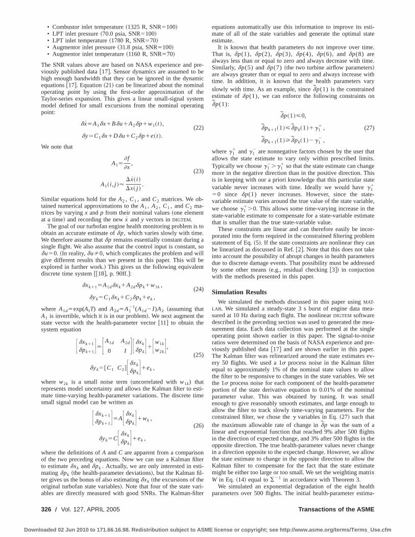
• Combustor inlet temperature~1325 R, SNR5100!• LPT inlet pressure~70.0 psia, SNR5100!• LPT inlet temperature~1780 R, SNR570!• Augmentor inlet pressure~31.8 psia, SNR5100!• Augmentor inlet temperature~1160 R, SNR570!

The SNR values above are based on NASA experience and pre-viously published data@17#. Sensor dynamics are assumed to behigh enough bandwidth that they can be ignored in the dynamicequations@17#. Equation~21! can be linearized about the nominaloperating point by using the first-order approximation of theTaylor-series expansion. This gives a linear small-signal systemmodel defined for small excursions from the nominal operatingpoint:

d x5A1dx1Bdu1A2dp1w1~ t !,(22)

dy5C1dx1Ddu1C2dp1e~ t !.

We note that

A15] f

]x,

(23)

A1~ i , j !'D x~ i !

Dx~ j !.

Similar equations hold for theA2 , C1 , andC2 matrices. We ob-tained numerical approximations to theA1 , A2 , C1 , andC2 ma-trices by varyingx andp from their nominal values~one elementat a time! and recording the newx andy vectors inDIGTEM.

The goal of our turbofan engine health monitoring problem is toobtain an accurate estimate ofdp, which varies slowly with time.We therefore assume thatdp remains essentially constant during asingle flight. We also assume that the control input is constant, sodu50. ~In reality,duÞ0, which complicates the problem and willgive different results than we present in this paper. This will beexplored in further work.! This gives us the following equivalentdiscrete time system@@18#, p. 90ff.#:

dxk115A1ddxk1A2ddpk1w1k ,(24)

dyk5C1dxk1C2dpk1ek ,

where A1d5exp(A1T) and A2d5A121(A1d2I )A2 ~assuming that

A1 is invertible, which it is in our problem!. We next augment thestate vector with the health-parameter vector@11# to obtain thesystem equation

F dxk11

dpk11G5FA1d A2d

0 IG F dxk

dpkG1Fw1k

w2kG ,

(25)

dyk5@C1 C2#F dxk

dpkG1ek ,

where w2k is a small noise term~uncorrelated withw1k) thatrepresents model uncertainty and allows the Kalman filter to esti-mate time-varying health-parameter variations. The discrete timesmall signal model can be written as

F dxk11

dpk11G5AF dxk

dpkG1wk ,

(26)

dyk5CF dxk

dpkG1ek ,

where the definitions ofA andC are apparent from a comparisonof the two preceding equations. Now we can use a Kalman filterto estimatedxk anddpk . Actually, we are only interested in esti-matingdpk ~the health-parameter deviations!, but the Kalman fil-ter gives us the bonus of also estimatingdxk ~the excursions of theoriginal turbofan state variables!. Note that four of the state vari-ables are directly measured with good SNRs. The Kalman-filter

equations automatically use this information to improve its esti-mate of all of the state variables and generate the optimal stateestimate.

It is known that health parameters do not improve over time.That is, dp(1), dp(2), dp(3), dp(4), dp(6), and dp(8) arealways less than or equal to zero and always decrease with time.Similarly, dp(5) anddp(7) ~the two turbine airflow parameters!are always greater than or equal to zero and always increase withtime. In addition, it is known that the health parameters varyslowly with time. As an example, sincedp(1) is the constrainedestimate ofdp(1), we canenforce the following constraints ondp(1):

dp~1!<0,

dpk11~1!<dpk~1!1g11 , (27)

dpk11~1!>dpk~1!2g12 ,

whereg11 andg1

2 are nonnegative factors chosen by the user thatallows the state estimate to vary only within prescribed limits.Typically we chooseg1

2.g11 so that the state estimate can change

more in the negative direction than in the positive direction. Thisis in keeping with our a priori knowledge that this particular statevariable never increases with time. Ideally we would haveg1

1

50 since dp(1) never increases. However, since the state-variable estimate varies around the true value of the state variable,we chooseg1

1.0. This allows some time-varying increase in thestate-variable estimate to compensate for a state-variable estimatethat is smaller than the true state-variable value.

These constraints are linear and can therefore easily be incor-porated into the form required in the constrained filtering problemstatement of Eq.~5!. If the state constraints are nonlinear they canbe linearized as discussed in Ref.@2#. Note that this does not takeinto account the possibility of abrupt changes in health parametersdue to discrete damage events. That possibility must be addressedby some other means~e.g., residual checking@3#! in conjuctionwith the methods presented in this paper.

Simulation ResultsWe simulated the methods discussed in this paper usingMAT-

LAB. We simulated a steady-state 3 s burst of engine data mea-sured at 10 Hz during each flight. The nonlinearDIGTEM softwaredescribed in the preceding section was used to generated the mea-surement data. Each data collection was performed at the singleoperating point shown earlier in this paper. The signal-to-noiseratios were determined on the basis of NASA experience and pre-viously published data@17# and are shown earlier in this paper.The Kalman filter was relinearized around the state estimates ev-ery 50 flights. We used a 1s process noise in the Kalman filterequal to approximately 1% of the nominal state values to allowthe filter to be responsive to changes in the state variables. We setthe 1s process noise for each component of the health-parameterportion of the state derivative equation to 0.01% of the nominalparameter value. This was obtained by tuning. It was smallenough to give reasonably smooth estimates, and large enough toallow the filter to track slowly time-varying parameters. For theconstrained filter, we chose theg variables in Eq.~27! such thatthe maximum allowable rate of change indp was the sum of alinear and exponential function that reached 9% after 500 flightsin the direction of expected change, and 3% after 500 flights in theopposite direction. The true health-parameter values never changein a direction opposite to the expected change. However, we allowthe state estimate to change in the opposite direction to allow theKalman filter to compensate for the fact that the state estimatemight be either too large or too small. We set the weighting matrixW in Eq. ~14! equal toS21 in accordance with Theorem 3.

We simulated an exponential degradation of the eight healthparameters over 500 flights. The initial health-parameter estima-



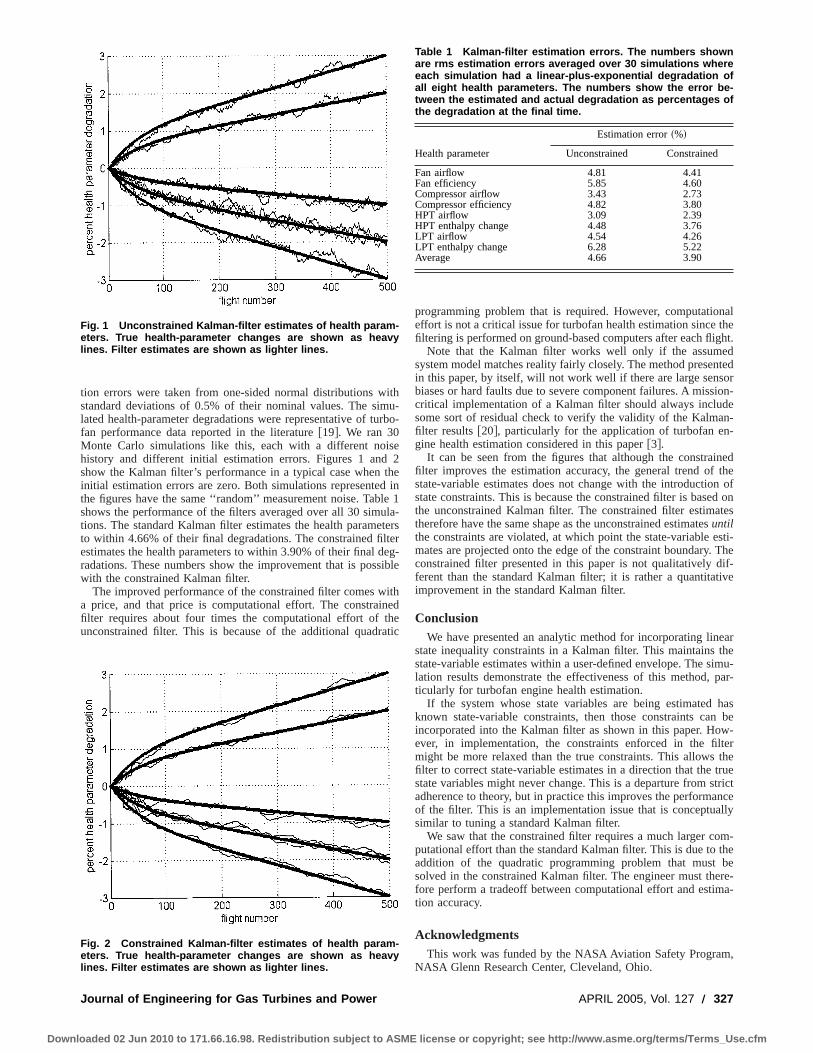
tion errors were taken from one-sided normal distributions withstandard deviations of 0.5% of their nominal values. The simu-lated health-parameter degradations were representative of turbo-fan performance data reported in the literature@19#. We ran 30Monte Carlo simulations like this, each with a different noisehistory and different initial estimation errors. Figures 1 and 2show the Kalman filter’s performance in a typical case when theinitial estimation errors are zero. Both simulations represented inthe figures have the same ‘‘random’’ measurement noise. Table 1shows the performance of the filters averaged over all 30 simula-tions. The standard Kalman filter estimates the health parametersto within 4.66% of their final degradations. The constrained filterestimates the health parameters to within 3.90% of their final deg-radations. These numbers show the improvement that is possiblewith the constrained Kalman filter.

The improved performance of the constrained filter comes witha price, and that price is computational effort. The constrainedfilter requires about four times the computational effort of theunconstrained filter. This is because of the additional quadratic

programming problem that is required. However, computationaleffort is not a critical issue for turbofan health estimation since thefiltering is performed on ground-based computers after each flight.

Note that the Kalman filter works well only if the assumedsystem model matches reality fairly closely. The method presentedin this paper, by itself, will not work well if there are large sensorbiases or hard faults due to severe component failures. A mission-critical implementation of a Kalman filter should always includesome sort of residual check to verify the validity of the Kalman-filter results@20#, particularly for the application of turbofan en-gine health estimation considered in this paper@3#.

It can be seen from the figures that although the constrainedfilter improves the estimation accuracy, the general trend of thestate-variable estimates does not change with the introduction ofstate constraints. This is because the constrained filter is based onthe unconstrained Kalman filter. The constrained filter estimatestherefore have the same shape as the unconstrained estimatesuntilthe constraints are violated, at which point the state-variable esti-mates are projected onto the edge of the constraint boundary. Theconstrained filter presented in this paper is not qualitatively dif-ferent than the standard Kalman filter; it is rather a quantitativeimprovement in the standard Kalman filter.

ConclusionWe have presented an analytic method for incorporating linear

state inequality constraints in a Kalman filter. This maintains thestate-variable estimates within a user-defined envelope. The simu-lation results demonstrate the effectiveness of this method, par-ticularly for turbofan engine health estimation.

If the system whose state variables are being estimated hasknown state-variable constraints, then those constraints can beincorporated into the Kalman filter as shown in this paper. How-ever, in implementation, the constraints enforced in the filtermight be more relaxed than the true constraints. This allows thefilter to correct state-variable estimates in a direction that the truestate variables might never change. This is a departure from strictadherence to theory, but in practice this improves the performanceof the filter. This is an implementation issue that is conceptuallysimilar to tuning a standard Kalman filter.

We saw that the constrained filter requires a much larger com-putational effort than the standard Kalman filter. This is due to theaddition of the quadratic programming problem that must besolved in the constrained Kalman filter. The engineer must there-fore perform a tradeoff between computational effort and estima-tion accuracy.

AcknowledgmentsThis work was funded by the NASA Aviation Safety Program,

NASA Glenn Research Center, Cleveland, Ohio.

Fig. 1 Unconstrained Kalman-filter estimates of health param-eters. True health-parameter changes are shown as heavylines. Filter estimates are shown as lighter lines.

Fig. 2 Constrained Kalman-filter estimates of health param-eters. True health-parameter changes are shown as heavylines. Filter estimates are shown as lighter lines.

Table 1 Kalman-filter estimation errors. The numbers shownare rms estimation errors averaged over 30 simulations whereeach simulation had a linear-plus-exponential degradation ofall eight health parameters. The numbers show the error be-tween the estimated and actual degradation as percentages ofthe degradation at the final time.

Health parameter

Estimation error~%!

Unconstrained Constrained

Fan airflow 4.81 4.41Fan efficiency 5.85 4.60Compressor airflow 3.43 2.73Compressor efficiency 4.82 3.80HPT airflow 3.09 2.39HPT enthalpy change 4.48 3.76LPT airflow 4.54 4.26LPT enthalpy change 6.28 5.22Average 4.66 3.90



References@1# Massicotte, D., Morawski, R., and Barwicz, A., 1995, ‘‘Incorporation of a

Positivity Constraint Into a Kalman-Filter-Based Algorithm for Correction ofSpectrometric Data,’’ IEEE Trans. Instrum. Meas.,44, pp. 2–7.

@2# Simon, D., and Chia, T., 2002, ‘‘Kalman Filtering With State Equality Con-straints,’’ IEEE Trans. Aerosp. Electron. Syst.,39, pp. 128–136.

@3# Doel, D., 1994, ‘‘TEMPER—A Gas-Path Analysis Tool for Commercial JetEngines,’’ ASME J. Eng. Gas Turbines Power,116, pp. 82–89.

@4# Doel, D., 1994, ‘‘An Assessment of Weighted-Least-Squares-Based Gas PathAnalysis,’’ ASME J. Eng. Gas Turbines Power,116, pp. 366–373.

@5# DePold, H., and Gass, F., 1999, ‘‘The Application of Expert Systems andNeural Networks to Gas Turbine Prognostics and Diagnostics,’’ ASME J. Eng.Gas Turbines Power,121, pp. 607–612.

@6# Volponi, A., DePold, H., Ganguli, R., and Chen, D., 2000, ‘‘The Use of Kal-man Filter and Neural Network Methodologies in Gas Turbine PerformanceDiagnostics: a Comparative Study,’’ ASME J. Eng. Gas Turbines Power,125,pp. 917–924.

@7# Kobayashi, T., and Simon, D. L., 2001, ‘‘A Hybrid Neural Network-GeneticAlgorithm Technique for Aircraft Engine Performance Diagnostics,’’ 37thAIAA/ASME/SAE/ASEE Joint Propulsion Conference, Salt Lake City, UT.

@8# Daniele, C., Krosel, S., Szuch, J., and Westerkamp, E., 1983, ‘‘Digital Com-puter Program for Generating Dynamic Turbofan Engine Models~DIGTEM!,’’NASA Technical Memorandum 83446.

@9# Szuch, J., Krosel, S., and Bruton, W., 1982, ‘‘Automated Procedure for Devel-oping Hybrid Computer Simulations of Turbofan Engines,’’ NASA TechnicalPaper 1851.

@10# Friedland, B., 1969, ‘‘Treatment of Bias in Recursive Filtering,’’ IEEE Trans.Autom. Control,AC14, pp. 359–367.

@11# Lambert, H., 1991, ‘‘A Simulation Study of Tubofan Engine DeteriorationEstimation Using Kalman Filtering Techniques,’’ NASA Technical Memoran-dum 104233.

@12# Roemer, M., and Kacprzynski, G., 2000, ‘‘Advanced Diagnostics and Prog-nostics for Turbine Engine Risk Assessment,’’ IEEE Aerospace Conference,Big Sky, MT., pp. 345–353.

@13# Anderson, B., and Moore, J., 1979,Optimal Filtering, Prentice-Hall, Engle-wood Cliffs, NJ.

@14# Fletcher, R., 1981,Practical Methods of Optimization, Vol. 2: ConstrainedOptimization, Wiley, New York.

@15# Gill, P., Murray, W., and Wright, M., 1981,Practical Optimization, Academic,New York.

@16# Daniele, C., and McLaughlin, P., 1984, ‘‘The Real-Time Performance of aParallel, Nonlinear Simulation Technique Applied to a Turbofan Engine,’’Modeling and Simulation on Microcomputers, R. Swartz, ed., Society forComputer Simulation, San Diego, CA, pp. 167–171.

@17# Merrill, W., 1984, ‘‘Identification of Multivariable High-Performance Turbo-fan Engine Dynamics From Closed-Loop Data,’’ J. Guid. Control Dyn.,7, pp.677–683.

@18# Chen, C., 1999,Linear System Theory and Design, Oxford University Press,New York.

@19# Sasahara, O., 1985, ‘‘JT9D Engine/Module Performance Deterioration ResultsFrom Back to Back Testing,’’ International Symposium on Air Breathing En-gines, Beijing, pp. 528–535.

@20# Gelb, A., 1974,Applied Optimal Estimation, MIT Press, Cambridge, MA.



Vellore P. Surender

Ranjan GanguliMem. ASME

Department of Aerospace Engineering,Indian Institute of Science,

Bangalore 650012, India

Adaptive Myriad Filter forImproved Gas Turbine ConditionMonitoring Using Transient DataThe removal of noise and outliers from measurement signals is a major problem in jetengine health monitoring. In this study, we look at the myriad filter as a substitute for themoving average filter that is widely used in the gas turbine industry. The three ideal testsignals used in this study are the step signal that simulates a single fault in the gasturbine, while ramp and quadratic signals simulate long term deterioration. Results showthat the myriad filter performs better in noise reduction and outlier removal when com-pared to the moving average filter. Further, an adaptive weighted myriad filter algorithmthat adapts to the quality of incoming data is studied. The filters are demonstrated onsimulated clean and deteriorated engine data obtained from an acceleration process fromidle to maximum thrust condition. This data was obtained from published literature andwas simulated using a transient performance prediction code. The deteriorated enginehad single component faults in the low pressure turbine and intermediate pressure com-pressor. The signals are obtained from T2 (IPC total outlet temperature) and T6 (LPTtotal outlet temperature) engine sensors with their nonrepeatability values that were usedas noise levels. The weighted myriad filter shows even greater noise reduction and outlierremoval when compared to the sample myriad and a FIR filter in the gas turbine diag-nosis. Adaptive filters such as those considered in this study are also useful for onlinehealth monitoring, as they can adapt to changes in quality of incoming data.@DOI: 10.1115/1.1850491#

IntroductionGas turbines are important and expensive mechanical systems

that are used for power generation and aircraft propulsion. Moni-toring the health of such systems is an important engineeringproblem. Aircraft jet engines are fitted with four basic measure-ments: low rotor speed, high rotor speed, exhaust gas temperature,and fuel flow rate. These measurements lead to four measurementdeviations or deltas that are the difference from the measurementsof the damaged engine and the undamaged or baseline engine.These measurement deltas are the health signals which are veryimportant for health monitoring since they contain informationabout the condition of the gas turbine engine@1,2#. A key problemin condition monitoring is the presence of high levels of noise andoutliers in the data. Another problem is the presence of suddentrend shifts in gas path measurements that can occur due to so-called ‘‘single faults’’ or repair events. It has been found from ananalysis of engine data that most faults in gas turbine engines arepreceded by a sudden increase in one or more measurements@3#.These ‘‘single faults’’ result in a step change in the gas path mea-surements. Besides ‘‘single faults,’’ gas turbines undergo deterio-ration over time, which shows up as a gradual increase in the gaspath measurement deltas. It has been found from a study of rev-enue service data that these measurements follow a low-orderpolynomial variation with respect to time and a linear approxima-tion is quite accurate@4–6#. Some studies have looked at derivingalgorithms for removing noise from gas turbine measurement del-tas. In @3#, the exponential average filter was suggested as analternative to the FIR moving average filter. The authors also sug-gest rules of thumb for removing outliers based on the logic that itis not physically possible for any one measurement to change and

for the other measurements to not change. Such points were clas-sified as outliers. Some studies have looked at median-type filtersfor denoising gas path health signals. However, these algorithmsare based on median-type filters and have a time delay@7,8#. Sincedata on aircraft power plants are obtained only once or twice perflight, the time delay is a handicap. Other researchers have lookedat neural network based approaches for denoising gas path healthsignals@9#.

The test signals used in this paper are for transient data. It ispossible to use both steady-state and transient data for diagnostics.However, good steady-state data may not be available under alloperating conditions. For example, military engines can operateup to 70% of the time in unsteady conditions@10#. In addition,some faults may be amplified under transient conditions. Severalauthors have looked at engine diagnostics with transient data@10–13#. Some studies address the problem of fault detection and a fewhave looked at the assessment of the fault magnitude. Neural net-work and genetic algorithms have been used for the fault isolationproblem. While the neural approach is robust to the presence ofsome level of noise in data, all fault isolation algorithms benefitfrom prior signal processing. Since transient data is acquired on-line at a reasonably high rate, we study an online adaptive signalprocessing method in this paper, which can be useful for datacleaning prior to fault isolation and visual display to humanengineers.

Linear filtering algorithms used in practical applications arelimited to the cases of Gaussian noise and show performance deg-radation in the presence of impulsive contamination. The class ofmyriad filters has been proposed for filtering highly noisy data@14–17#. In this study, we look at the myriad filter as a substitutefor the moving average filter that is widely used in the gas turbineindustry.

Myriad FilterMyriad filters are nonlinear filters whose development was mo-

tivated by the properties ofa-stable distributions, a family ofheavy-tailed densities that have been proposed for robust non-

Contributed by the International Gas Turbine Institute~IGTI! of THE AMERICANSOCIETY OF MECHANICAL ENGINEERSfor publication in the ASME JOURNAL OFENGINEERING FOR GAS TURBINES AND POWER. Paper presented at the Interna-tional Gas Turbine and Aeroengine Congress and Exhibition, Vienna, Austria, June13–17, 2004, Paper No. 2004-GT-53080. Manuscript received by IGTI, October 1,2003; final revision, March 1, 2004. IGTI Review Chair: A. J. Strazisar.



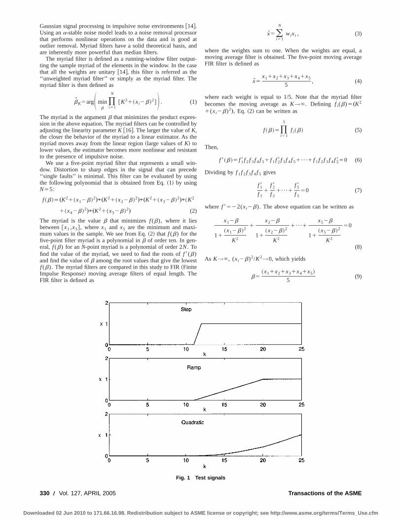
Gaussian signal processing in impulsive noise environments@14#.Using ana-stable noise model leads to a noise removal processorthat performs nonlinear operations on the data and is good atoutlier removal. Myriad filters have a solid theoretical basis, andare inherently more powerful than median filters.

The myriad filter is defined as a running-window filter output-ting the sample myriad of the elements in the window. In the casethat all the weights are unitary@14#, this filter is referred as the‘‘unweighted myriad filter’’ or simply as the myriad filter. Themyriad filter is then defined as

bK5argS minb

)i 51

N

@K21~xi2b!2# D . (1)

The myriad is the argumentb that minimizes the product expres-sion in the above equation. The myriad filters can be controlled byadjusting the linearity parameterK @16#. The larger the value ofK,the closer the behavior of the myriad to a linear estimator. As themyriad moves away from the linear region~large values ofK! tolower values, the estimator becomes more nonlinear and resistantto the presence of impulsive noise.

We use a five-point myriad filter that represents a small win-dow. Distortion to sharp edges in the signal that can precede‘‘single faults’’ is minimal. This filter can be evaluated by usingthe following polynomial that is obtained from Eq.~1! by usingN55:

f ~b!5„K21~x12b!2…* „K21~x22b!2

…* „K21~x32b!2…* ~K2

1~x42b!2…* „K21~x52b!2

… (2)

The myriad is the valueb that minimizes f (b), where it liesbetween@x1 ,x5#, wherex1 and x5 are the minimum and maxi-mum values in the sample. We see from Eq.~2! that f (b) for thefive-point filter myriad is a polynomial inb of order ten. In gen-eral, f (b) for anN-point myriad is a polynomial of order 2N. Tofind the value of the myriad, we need to find the roots off 8(b)and find the value ofb among the root values that give the lowestf (b). The myriad filters are compared in this study to FIR~FiniteImpulse Response! moving average filters of equal length. TheFIR filter is defined as

x5(i 51

N

wixi , (3)

where the weights sum to one. When the weights are equal, amoving average filter is obtained. The five-point moving averageFIR filter is defined as

x5x11x21x31x41x5

5, (4)

where each weight is equal to 1/5. Note that the myriad filterbecomes the moving average asK→`. Defining f i(b)5„K2

1(xi2b)2…, Eq. ~2! can be written as

f ~b!5)i 51

5

f i~b! (5)

Then,

f 8~b!5 f 18 f 2f 3f 4f 51 f 1f 28 f 3f 4f 51¯1 f 1f 2f 3f 4f 5850 (6)

Dividing by f 1f 2f 3f 4f 5 gives

f 18

f 11

f 28

f 21¯1

f 58

f 550 (7)

where f 8522(xi2b). The above equation can be written as

x12b

11~x12b!2

K2

1x22b

11~x22b!2

K2

1¯1x52b

11~x52b!2

K2

50

(8)

As K→`, (xi2b)2/K2→0, which yields

b5~x11x21x31x41x5!

5(9)

Fig. 1 Test signals



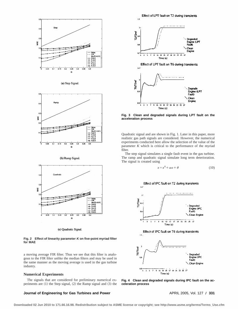
a moving average FIR filter. Thus we see that this filter is analo-gous to the FIR filter unlike the median filters and may be used inthe same manner as the moving average is used in the gas turbineindustry.

Numerical ExperimentsThe signals that are considered for preliminary numerical ex-

periments are~1! the Step signal,~2! the Ramp signal and~3! the

Quadratic signal and are shown in Fig. 1. Later in this paper, morerealistic gas path signals are considered. However, the numericalexperiments conducted here allow the selection of the value of theparameterK which is critical to the performance of the myriadfilter.

The step signal simulates a single fault event in the gas turbine.The ramp and quadratic signal simulate long term deterioration.The signal is created using

x5x01a«1u (10)

Fig. 2 Effect of linearity parameter K on five-point myriad filterfor MAE

Fig. 3 Clean and degraded signals during LPT fault on theacceleration process

Fig. 4 Clean and degraded signals during IPC fault on the ac-celeration process



wherex0 is the root signal,« accounts for Gaussian noise andufor non-Gaussian outliers. Herea is a parameter called noise levelthat allows us to control the level of noise in the data. AC filterperforms the following operations that returns the filtered signalfrom the corrupted signal.

y5C~x!5C~x01ae1u! (11)

The following error measures will be used to analyze the myriadfilter performance over a sample ofN points by comparing thefiltered signal with the root signal

MAE5(i 51

Nu~y2x0!u

N(12)

Fig. 5 Clean and degraded signals during LPT fault on the acceleration pro-cess for T2



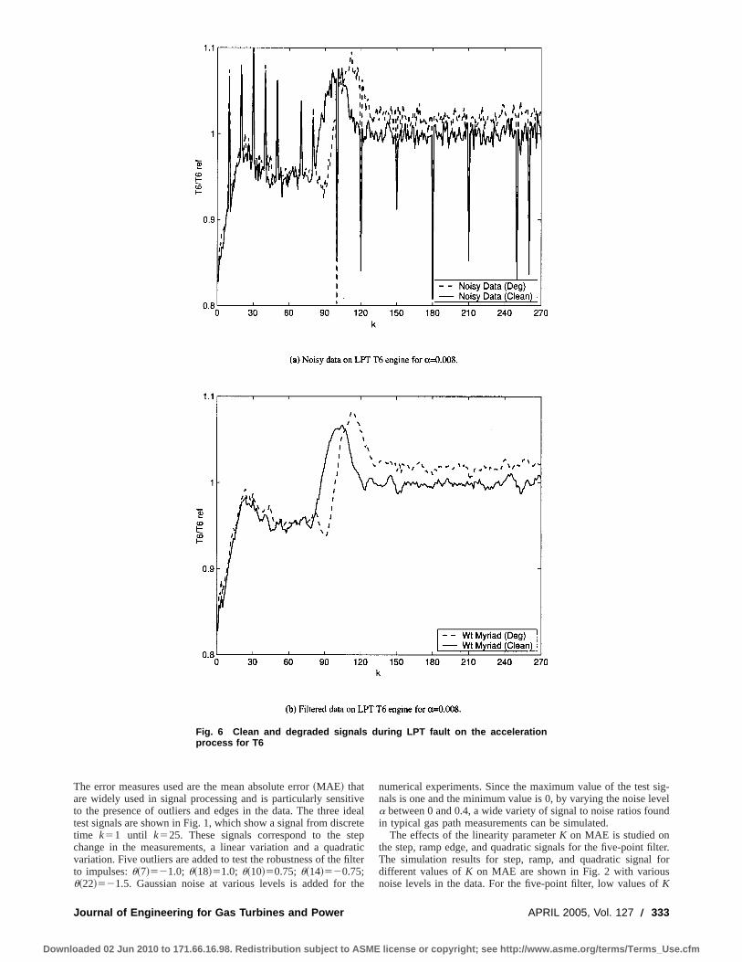
The error measures used are the mean absolute error~MAE! thatare widely used in signal processing and is particularly sensitiveto the presence of outliers and edges in the data. The three idealtest signals are shown in Fig. 1, which show a signal from discretetime k51 until k525. These signals correspond to the stepchange in the measurements, a linear variation and a quadraticvariation. Five outliers are added to test the robustness of the filterto impulses:u~7!521.0; u~18!51.0; u~10!50.75; u~14!520.75;u~22!521.5. Gaussian noise at various levels is added for the

numerical experiments. Since the maximum value of the test sig-nals is one and the minimum value is 0, by varying the noise levela between 0 and 0.4, a wide variety of signal to noise ratios foundin typical gas path measurements can be simulated.

The effects of the linearity parameterK on MAE is studied onthe step, ramp edge, and quadratic signals for the five-point filter.The simulation results for step, ramp, and quadratic signal fordifferent values ofK on MAE are shown in Fig. 2 with variousnoise levels in the data. For the five-point filter, low values ofK

Fig. 6 Clean and degraded signals during LPT fault on the accelerationprocess for T6



~such asK50.01) cause the myriad performance to become worsethan the FIR at higher noise levels. For high values ofK such asK55, the myriad filter approaches the FIR filter in performance.Since gas path signals have reasonably low levels of noise andhave more possibility for outlier contamination, a value ofK50.1 is selected.

Gas Turbine Transient SignalThe trajectories for a clean and deteriorated engine are pre-

sented during an acceleration process. The deteriorated engine had

single component faults in LPT~low pressure turbine! and IPC~intermediate pressure compressor! implanted, respectively. Thesignals of LPT fault and IPC fault on T2 and T6 during transientsare obtained from@18#. These ideal signals are shown in Fig. 3and Fig. 4.

The noise levela of 0.004 is the level of noise used in@18#. Weuse a50.004 anda50.008 to simulate conditions with normaldata and low quality data, respectively. Outliers are also added tothe signals. The noisy signals are shown in Figs. 5~a!, 6~a! and7~a!. Tables 1–2 show the MAE values on the T2 measurements.

Fig. 7 Clean and degraded signals during IPC fault on the acceleration pro-cess for T2



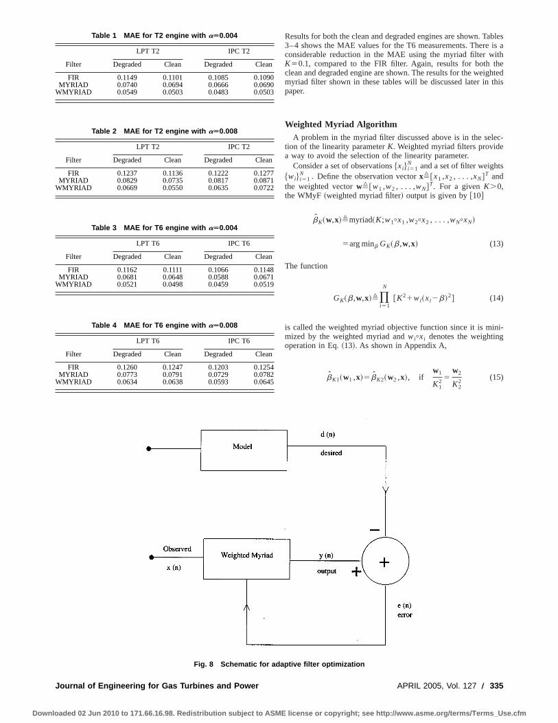
Results for both the clean and degraded engines are shown. Tables3–4 shows the MAE values for the T6 measurements. There is aconsiderable reduction in the MAE using the myriad filter withK50.1, compared to the FIR filter. Again, results for both theclean and degraded engine are shown. The results for the weightedmyriad filter shown in these tables will be discussed later in thispaper.

Weighted Myriad AlgorithmA problem in the myriad filter discussed above is in the selec-

tion of the linearity parameterK. Weighted myriad filters providea way to avoid the selection of the linearity parameter.

Consider a set of observations$xi% i 51N and a set of filter weights

$wi% i 51N . Define the observation vectorx,@x1 ,x2 , . . . ,xN#T and

the weighted vectorw,@w1 ,w2 , . . . ,wN#T. For a givenK.0,the WMyF ~weighted myriad filter! output is given by@10#

bK~w,x!,myriad~K;w1+x1 ,w2+x2 , . . . ,wN+xN!

5arg minb GK~b,w,x! (13)

The function

GK~b,w,x!,)i 51

N

@K21wi~xi2b!2# (14)

is called the weighted myriad objective function since it is mini-mized by the weighted myriad andwi+xi denotes the weightingoperation in Eq.~13!. As shown in Appendix A,

bK1~w1 ,x!5bK2~w2 ,x!, ifw1

K12

5w2

K22

(15)

Fig. 8 Schematic for adaptive filter optimization

Table 1 MAE for T2 engine with aÄ0.004

Filter

LPT T2 IPC T2

Degraded Clean Degraded Clean

FIR 0.1149 0.1101 0.1085 0.1090MYRIAD 0.0740 0.0694 0.0666 0.0690

WMYRIAD 0.0549 0.0503 0.0483 0.0503


Filter

LPT T2 IPC T2


FIR 0.1237 0.1136 0.1222 0.1277MYRIAD 0.0829 0.0735 0.0817 0.0871

WMYRIAD 0.0669 0.0550 0.0635 0.0722


Filter

LPT T6 IPC T6


FIR 0.1162 0.1111 0.1066 0.1148MYRIAD 0.0681 0.0648 0.0588 0.0671

WMYRIAD 0.0521 0.0498 0.0459 0.0519


Filter

LPT T6 IPC T6


FIR 0.1260 0.1247 0.1203 0.1254MYRIAD 0.0773 0.0791 0.0729 0.0782

WMYRIAD 0.0634 0.0638 0.0593 0.0645



Thus the filter output depends onw/K2. Thus the problem offinding the optimal linearity parameterK is avoided by using theweighted myriad filter. However, the problem of finding the ap-propriate value ofK is now replaced by finding the appropriateweight vector. In general, the myriad is the global minima amongseveral local minimum points ofG(b). To compute the myriad,one needs to find the roots of polynomialG8(b), and test all thelocal minima to find the global minima.

Adaptive Weighted Myriad Filter Algorithm

For applications where the statistics of the signal are unknownor time varying, the adaptive algorithm is very useful. For gaspath measurements, historical data is often used to obtain repre-sentative numbers for measurement uncertainty. However, it islikely that the uncertainty changes for different outliers and en-gines and for different operating conditions. The adaptive algo-

Fig. 9 A comparison of filters



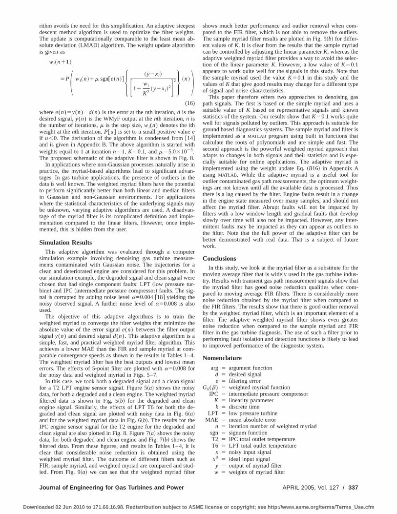
rithm avoids the need for this simplification. An adaptive steepestdescent method algorithm is used to optimize the filter weights.The update is computationally comparable to the least mean ab-solute deviation~LMAD ! algorithm. The weight update algorithmis given as

wi~n11!

5PS wi~n!1m sgn@e~n!#H ~y2xi !

F11wi

K2~y2xi !

2G 2J ~n!D(16)

wheree(n)5y(n)2d(n) is the error at the nth iteration,d is thedesired signal,y(n) is the WMyF output at thenth iteration,n isthe number of iterations,m is the step size,wi(n) denotes theithweight at thenth iteration,P@u# is set to a small positive value«if u,0. The derivation of the algorithm is condensed from@14#and is given in Appendix B. The above algorithm is started withweights equal to 1 at iterationn51, K50.1, andm55.031023.The proposed schematic of the adaptive filter is shown in Fig. 8.

In applications where non-Gaussian processes naturally arise inpractice, the myriad-based algorithms lead to significant advan-tages. In gas turbine applications, the presence of outliers in thedata is well known. The weighted myriad filters have the potentialto perform significantly better than both linear and median filtersin Gaussian and non-Gaussian environments. For applicationswhere the statistical characteristics of the underlying signals maybe unknown, varying adaptive algorithms are used. A disadvan-tage of the myriad filter is its complicated definition and imple-mentation compared to the linear filters. However, once imple-mented, this is hidden from the user.

Simulation ResultsThis adaptive algorithm was evaluated through a computer

simulation example involving denoising gas turbine measure-ments contaminated with Gaussian noise. The trajectories for aclean and deteriorated engine are considered for this problem. Inour simulation example, the degraded signal and clean signal werechosen that had single component faults: LPT~low pressure tur-bine! and IPC~intermediate pressure compressor! faults. The sig-nal is corrupted by adding noise levela50.004@18# yielding thenoisy observed signal. A further noise level ofa50.008 is alsoused.

The objective of this adaptive algorithms is to train theweighted myriad to converge the filter weights that minimize theabsolute value of the error signale(n) between the filter outputsignaly(n) and desired signald(n). This adaptive algorithm is asimple, fast, and practical weighted myriad filter algorithm. Thisachieves a lower MAE than the FIR and sample myriad at com-parable convergence speeds as shown in the results in Tables 1–4.The weighted myriad filter has the best outputs and lowest meanerrors. The effects of 5-point filter are plotted witha50.008 forthe noisy data and weighted myriad in Figs. 5–7.

In this case, we took both a degraded signal and a clean signalfor a T2 LPT engine sensor signal. Figure 5~a! shows the noisydata, for both a degraded and a clean engine. The weighted myriadfiltered data is shown in Fig. 5~b! for the degraded and cleanengine signal. Similarly, the effects of LPT T6 for both the de-graded and clean signal are plotted with noisy data in Fig. 6~a!and for the weighted myriad data in Fig. 6~b!. The results for theIPC engine sensor signal for the T2 engine for the degraded andclean signal are also plotted in Fig. 8. Figure 7~a! shows the noisydata, for both degraded and clean engine and Fig. 7~b! shows thefiltered data. From these figures, and results in Tables 1–4, it isclear that considerable noise reduction is obtained using theweighted myriad filter. The outcome of different filters such asFIR, sample myriad, and weighted myriad are compared and stud-ied. From Fig. 9~a! we can see that the weighted myriad filter

shows much better performance and outlier removal when com-pared to the FIR filter, which is not able to remove the outliers.The sample myriad filter results are plotted in Fig. 9~b! for differ-ent values ofK. It is clear from the results that the sample myriadcan be controlled by adjusting the linear parameterK, whereas theadaptive weighted myriad filter provides a way to avoid the selec-tion of the linear parameterK. However, a low value ofK50.1appears to work quite well for the signals in this study. Note thatthe sample myriad used the valueK50.1 in this study and thevalues ofK that give good results may change for a different typeof signal and noise characteristics.

This paper therefore offers two approaches to denoising gaspath signals. The first is based on the simple myriad and uses asuitable value ofK based on representative signals and knownstatistics of the system. Our results show thatK50.1 works quitewell for signals polluted by outliers. This approach is suitable forground based diagnostics systems. The sample myriad and filter isimplemented as aMATLAB program using built in functions thatcalculate the roots of polynomials and are simple and fast. Thesecond approach is the powerful weighted myriad approach thatadapts to changes in both signals and their statistics and is espe-cially suitable for online applications. The adaptive myriad isimplemented using the weight update Eq.~B16! in Appendix Ausing MATLAB . While the adaptive myriad is a useful tool foroutlier contaminated gas path measurements, the optimum weight-ings are not known until all the available data is processed. Thusthere is a lag caused by the filter. Engine faults result in a changein the engine state measured over many samples, and should notaffect the myriad filter. Abrupt faults will not be impacted byfilters with a low window length and gradual faults that developslowly over time will also not be impacted. However, any inter-mittent faults may be impacted as they can appear as outliers tothe filter. Note that the full power of the adaptive filter can bebetter demonstrated with real data. That is a subject of futurework.

ConclusionsIn this study, we look at the myriad filter as a substitute for the

moving average filter that is widely used in the gas turbine indus-try. Results with transient gas path measurement signals show thatthe myriad filter has good noise reduction qualities when com-pared to moving average FIR filters. There is considerably morenoise reduction obtained by the myriad filter when compared tothe FIR filters. The results show that there is good outlier removalby the weighted myriad filter, which is an important element of afilter. The adaptive weighted myriad filter shows even greaternoise reduction when compared to the sample myriad and FIRfilter in the gas turbine diagnosis. The use of such a filter prior toperforming fault isolation and detection functions is likely to leadto improved performance of the diagnostic system.

Nomenclature

arg 5 argument functiond 5 desired signale 5 filtering error

Gk(b) 5 weighted myriad functionIPC 5 intermediate pressure compressor

K 5 linearity parameterk 5 discrete time

LPT 5 low pressure turbineMAE 5 mean absolute error

n 5 iteration number of weighted myriadsgn 5 signum functionT2 5 IPC total outlet temperatureT6 5 LPT total outlet temperature

x 5 noisy input signalx0 5 ideal input signaly 5 output of myriad filterw 5 weights of myriad filter



a 5 noise level« 5 Gaussian noise

bk 5 sample myriadm 5 step sizeu 5 non-Gaussian outliers

Appendix A: Filter Weights and the LinearityParameter

Using negative weights results in the potential instability of thefilter so it is defined using positive weights:wi>0, i51,2, . . . ,N. The WMyf output is the value ofb at its globalminimum of GK(b). For wi>0 and K.0, G(b).0 for all b.Furthermore,GK(b) is a polynomial inb of degree 2N. Themyriad b is defined as the minimum value ofGK(b) and occursat one of the roots ofGK8 (b),

GK8 ~ b !50. (A1)

Differentiating ~8! gives

GK8 ~b!5(j 51

N

2wj~b2xj !)l 51lÞ j

N

@K21wl~b2xl !2# (A2)

which is a polynomial of degree 2N21 with as many as 2N21real roots. Using~8! and ~12!, we get

GK8 ~b!52GK8 ~b!(j 51

Nwj~b2xj !

K21wj~b2xj !2

(A3)

SinceGK8 (b).0, the filter outputb must satisfy

(j 51

N

wj

K2~ b2xj !

11wj

K2~ b2xj !

2

50 (A4)

The above equation shows that even if the value ofK is changedthe same filter output is obtained provided the weights are suitablyscaled. Therefore,

bK1~w1 ,x!5bK2~w2 ,x! ifw1

K12

5w2

K22

(A5)

Appendix B: Optimal Filter WeightsIn order to find the optimal weights, the steepest descent

method can be used to minimize the MAE cost functionJ(w) @14#where

J~w,K !5E$uyK~w,x!2du% (B1)

andE$•% is the statistical expectation andd is the desired signal.Hered can be generated by an onboard model of the engine. Thefollowing algorithm is used to update the filter weights

wi~n11!5PFwi~n!2m]J

]wi~n!G (B2)

wherewi(n) denotes theith weight at thenth iteration,m.0 is thestep size of the update, andP@•# is defined as

P@u#,u, u.0(B3)

0, u<0

In practiceP@u# is set to a small positive valuee if u<0. Differ-entiating„Eq. ~A5!… we obtain;

]J

]wi~n!5EH sgn@y~n!2d~n!#

]y

]wi~n!J (B4)

Since a lack of knowledge of signal statistics makes evaluation ofstatistical expectationE difficult, an instantaneous estimate for thegradient is used. Putting„Eq. ~B3!… into „Eq. ~B2!… yields,

wi~n11!5PH wi~n!2m sgn@e~n!#]y

]wi~n!J (B5)

wheree(n)5y(n)2d(n) is the error at thenth iteration. To find]y/]wi for a givenK, we can write Eq.~A1! as

GK8 ~y!52GK~y,w,x!(j 51

Nwj~y2xj !

K21wj~y2xj !2

(B6)

ConsiderK; the other weights and input vectorx are constant.Then,

G8~y!52G~y,wi !H~y,wi ! (B7)

where

H~y,wi !,(j 51

Nwj~y2xj !

K21wj~y2xj !2

(B8)

SinceG8(y)50,

G~y,wi !H~y,wi !50 (B9)

SinceG(y,wi)>0,

H~y,wi !50 (B10)

Differentiating the above equation with respect towi yields

]H

]y•

]y

]wi1

]H

]wi50

]y

]wi52

]H

]wi

]H

]y

(B11)

]H

]wi5

]

]wi(j 51

Nwj~y2xj !

K21wj~y2xj !2

51

K2 H ~y2xi !

F11wj

K2~y2xi !

2G 2J(B12)

]H

]y5

]

]y (j 51

Nwj~y2xj !

K21wj~y2xj !2

5(j 51

Nwj

K2•

12wj

K2~y2xj !

2

F11wj

K2~y2xj !

2G 2

(B13)

Putting Eq.~B12! and Eq.~B11! in Eq. ~B10! we get

]y

]wi5

H 2~y2xi !

F11wj

K2~y2xi !

2G 2JK25 (

j 51

Nwj

K2

12wj

K2~y2xj !

2

F11wj

K2~y2xj !

2G 26(B14)

Putting Eq.~A5! into Eq. ~A4! and adding a stability constantayields



wi~n11!5PS wi~n!1m sgn@e~n!#

H ~y2xi !

F11wj

K2~y2xi !

2G 2J ~n!

K25 a1(j 51

Nwj

K2

12wj

K2~y2xj !

2

F11wj

K2~y2xj !

2G 26 ~n!D (B15)

We can remove the denominator from the update term in the above equation as it does not effect the direction of the gradient estimateor the values of the final weights. This leads to

wi~n11!5PS wi~n!1m sgn@e~n!#H ~y2xi !

F11wj

K2~y2xi !

2G 2J ~n!D (B16)

References@1# Volponi, A. J., and Urban, L. A., 1992, ‘‘Mathematical Methods of Relative

Engine Performances Diagnostics,’’ SAE Trans., Journal of Aerospace Techni-cal Paper 922048, p. 101.

@2# Doel, D. L., 2003, ‘‘Interpretation of Weighted-Least-Squares Gas Path Analy-sis Results,’’ J. Eng. Gas Turbines Power,125, pp. 624–633.

@3# DePold, H., and Gass, F. D., 1999, ‘‘The Application of Expert Systems andNeural Network to Gas Turbine Prognostics and Diagnostics,’’ J. Eng. GasTurbines Power,121, pp. 607–612.

@4# Fasching, W. A., and Stricklin, R., 1982, CF6 Jet Engine Diagnostics Program,Final Report 1, NASA/CR-165582.

@5# Glenny, D. E., 1988, ‘‘Gas Path Analysis and Engine Performance Monitoringin a Chinook Helicopter,’’ Paper 25 AGARD-CP-448 1, Engine ConditionMonitoring Technology and Experience.

@6# Mathioudakis, K., Kamboukos, P. H., and Stamatis, A., 2002, ‘‘Turbofan Per-formance Deterioration Tracking Using Non-Linear Models and OptimizationTechniques,’’ J. Turbomach.,124, pp. 580–587.

@7# Ganguli, R., 2002, ‘‘Noise and Outlier Removal From Jet Engine Health Sig-nals Using Weighted FIR Median Hybrid Filters,’’ Mech. Syst. Signal Process.,16, pp. 967–978.

@8# Ganguli, R., 2003, ‘‘Jet Engine Gas Path Measurement Filtering Using CenterWeighted Idempotent Median Filters,’’ J. Propul. Power,19, pp. 930–937.

@9# Lu, P. J., and Hsu, T. C., 2002, ‘‘Application of Autoassociative Neural Net-work on Gas-Path Sensor Data Validation,’’ J. Propul. Power,18, pp. 879–888.

@10# Li, Y. G., 2003, ‘‘A Gas Turbine Diagnostic Approach With Transient Mea-

surements,’’ Proc. Inst. Mech. Eng., Part A, J. Power Energy,217, pp. 169–177.

@11# Eustace, R. W., Woodyatt, B. A., Merrington, G. L., and Runacres, A., 1994,‘‘Fault Signatures Obtained From Fault Implant Tests on an F404 Engine,’’ J.Eng. Gas Turbines Power,116, pp. 178–183.

@12# Merrington, G. L., 1988, ‘‘Identification of Dynamic Characteristics for FaultIsolation Purposes in a Gas Turbine Using Closed-Loop Measurements,’’En-gine Condition Monitoring-Technology and Experience, AGARD-CP-448.

@13# Merrington, G. L., 1994, ‘‘Fault Diagnosis in Gas Turbines Using a Model-Based Technique,’’ J. Eng. Gas Turbines Power,116, pp. 374–380.

@14# Kalluri, S., and Arce, G. R., 1998, ‘‘Adaptive Weighted Myriad Filter Algo-rithms for Robust Signal Processing in Alpha-Stable Noise Environments,’’IEEE Trans. Signal Process.,46, pp. 322–334.

@15# Gonzalez, J. G., and Arce, G. R., 2002, ‘‘Statistically-Efficient Filtering inImpulsive Environments: Weighted Myriad Filters,’’ EURASIP J. Appli. Sig-nal Process.,1, pp. 4–20.

@16# Gonzalez, J. G., and Arce, G. R., 2001, ‘‘Optimality for the Myriad Filter inPractical Impulsive-Noise Environments,’’ IEEE Trans. Signal Process.,49,pp. 438–441.

@17# Kalluri, S., and Arce, G. R., 2000, ‘‘Fast Algorithm for Weighted MyriadComputation by Fixed Point Search,’’ IEEE Trans. Signal Process.,48, pp.159–171.

@18# Ogaji, S. O. T., Li, Y. G., Sampath, S., and Singh, R., ‘‘Gas Path Fault Diag-nosis of a Turbofan Engine From Transient Data Using Artificial Neural Net-works,’’ ASME Paper GT2003-38423.



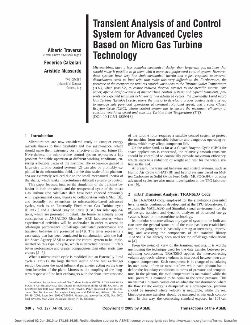
Alberto Traversoe-mail: [email protected]

Federico Calzolari

Aristide Massardo

TPG-DiMSET,Universita di Genova,

Genova, Italy

Transient Analysis of and ControlSystem for Advanced CyclesBased on Micro Gas TurbineTechnologyMicroturbines have a less complex mechanical design than large-size gas turbines thatshould make it possible to fit them with a more straightforward control system. However,these systems have very low shaft mechanical inertia and a fast response to externaldisturbances, such as load trip, that make this very difficult to do. Furthermore, thepresence of the recuperator requires smooth variations to the Turbine Outlet Temperature(TOT), when possible, to ensure reduced thermal stresses to the metallic matrix. Thispaper, after a brief overview of microturbine control systems and typical transients, pre-sents the expected transient behavior of two advanced cycles: the Externally Fired microGas Turbine (EFmGT) cycle, where the aim is to develop a proper control system set-upto manage safe part-load operations at constant rotational speed, and a solar ClosedBrayton Cycle (CBC), whose control system has to ensure the maximum efficiency atconstant rotational speed and constant Turbine Inlet Temperature (TIT).@DOI: 10.1115/1.1839918#

1 Introduction

Microturbines are now considered ready to conquer energymarkets thanks to their flexibility and low maintenance, whichshould make them extremely cost effective in the near future@1#.Nevertheless, the microturbine control system represents a keyproblem for stable operation at different working conditions, en-suring a flexible usage of the machine. The experience gained inlarge-size turbine control systems@2# can also be profitably ex-ploited in the microturbine field, but the time scale of the phenom-ena are extremely reduced due to the small mechanical inertia ofthe shafts, which make microturbines difficult systems to control.

This paper focuses, first, on the simulation of the transient be-havior in both the simple and the recuperated cycle of the microGas Turbine~the calculated data have been checked previouslywith experimental ones, thanks to collaboration with ENEL@3#!,and secondly, on extensions to microturbine-based advancedcycles, such as an Externally Fired micro Gas Turbine cycle~EFmGT! and a Closed Brayton Cycle~CBC! for solar applica-tions, which are presented in detail. The former is actually underconstruction at ANSALDO Ricerche~ARI! laboratories, whereexperimental activities will be undertaken in order to assess itsoff-design performance~off-design calculated performance andtransient behavior are presented in@4#!. The latter represents acase-study that has been conducted in collaboration with the Ital-ian Space Agency~ASI! to assess the control system to be imple-mented on this type of cycle, which is attractive because it offersbetter performance and greater compactness than other static gen-erators@5–7#.

When a microturbine cycle is modified into an Externally Firedcycle ~EFmGT!, the large thermal inertia of the heat exchangersection becomes the most influential parameter acting on the tran-sient behavior of the plant. Moreover, the coupling of the long-term response of the heat exchangers with the short-term response

of the turbine rotor requires a suitable control system to protectthe machine from unstable behavior and dangerous operating re-gions, which may affect component life.

On the other hand, as far as a Closed Brayton Cycle~CBC! forspace applications is concerned, the relatively smooth transientsshould be controlled to continually provide maximum efficiency,which leads to a reduction of weight and cost for the whole sys-tem in the end.

At present, the transient behavior and control systems, such asHumid Air Cycle ~mHAT! @8# and hybrid systems based on Mol-ten Carbonate or Solid Oxide Fuel Cells~MCFC-SOFC!, of otheradvanced cycles are also under investigation at the TPG laborato-ries @9#.

2 mGT Transient Analysis: TRANSEO CodeThe TRANSEO code, employed for the simulations presented

here, is under continuous development at the TPG laboratories. Itexploits the MATLAB© and Simulink visual environment for theoff-design, transient and dynamic analyses of advanced energysystems based on microturbine technology.

Its modular structure allows any type of system to be built andrun: now the general structure of the code has been established,and the on-going work is basically aiming at increasing, improv-ing, and assessing the components of the standard library.TRANSEO has already been used for the off-design calculationsin @4#.

From the point of view of the transient analysis, it is worthymentioning the technique used for the data transfer between twoadjoining components. TRANSEO applies the interconnectingvolume approach, where a volume is interposed between two con-sequent components. Each component is in charge of calculatingits own mass inflow or mass outflow, while each plenum has todefine the boundary conditions in terms of pressure and tempera-ture. In the plenum, the total temperature is maintained while thetotal pressure is assumed to be equal to the static pressure. Thismeans that a plenum carries out an adiabatic transformation wherethe flow kinetic energy is dissipated: as a consequence, plenumsshould be inserted where velocity is negligible, while the realkinetic-pressure transfers should be managed within each compo-nent. In this way, the connecting standard exposed in@10# can




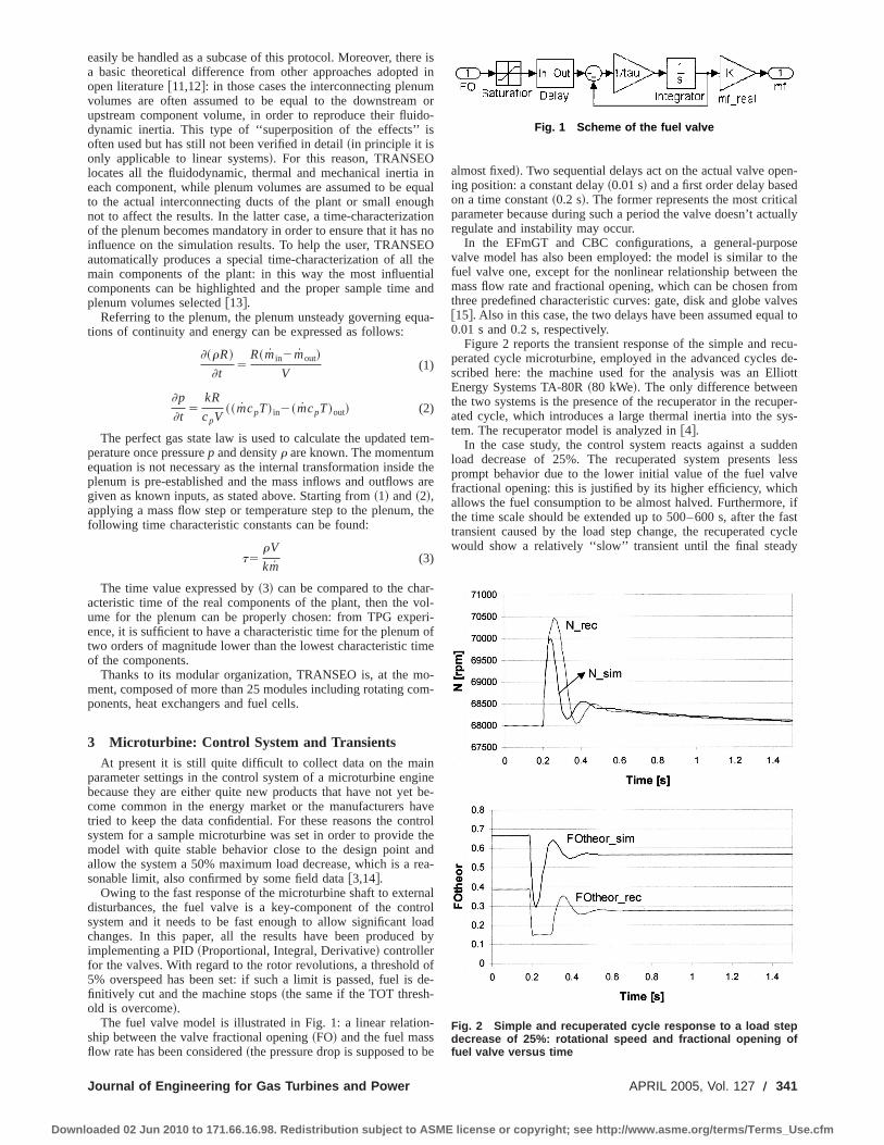
easily be handled as a subcase of this protocol. Moreover, there isa basic theoretical difference from other approaches adopted inopen literature@11,12#: in those cases the interconnecting plenumvolumes are often assumed to be equal to the downstream orupstream component volume, in order to reproduce their fluido-dynamic inertia. This type of ‘‘superposition of the effects’’ isoften used but has still not been verified in detail~in principle it isonly applicable to linear systems!. For this reason, TRANSEOlocates all the fluidodynamic, thermal and mechanical inertia ineach component, while plenum volumes are assumed to be equalto the actual interconnecting ducts of the plant or small enoughnot to affect the results. In the latter case, a time-characterizationof the plenum becomes mandatory in order to ensure that it has noinfluence on the simulation results. To help the user, TRANSEOautomatically produces a special time-characterization of all themain components of the plant: in this way the most influentialcomponents can be highlighted and the proper sample time andplenum volumes selected@13#.

Referring to the plenum, the plenum unsteady governing equa-tions of continuity and energy can be expressed as follows:

]~rR!

]t5

R~min2mout!

V(1)

]p

]t5

kR

cpV~~mcpT! in2~mcpT!out! (2)

The perfect gas state law is used to calculate the updated tem-perature once pressurep and densityr are known. The momentumequation is not necessary as the internal transformation inside theplenum is pre-established and the mass inflows and outflows aregiven as known inputs, as stated above. Starting from~1! and~2!,applying a mass flow step or temperature step to the plenum, thefollowing time characteristic constants can be found:

t5rV

km(3)

The time value expressed by~3! can be compared to the char-acteristic time of the real components of the plant, then the vol-ume for the plenum can be properly chosen: from TPG experi-ence, it is sufficient to have a characteristic time for the plenum oftwo orders of magnitude lower than the lowest characteristic timeof the components.

Thanks to its modular organization, TRANSEO is, at the mo-ment, composed of more than 25 modules including rotating com-ponents, heat exchangers and fuel cells.

3 Microturbine: Control System and TransientsAt present it is still quite difficult to collect data on the main

parameter settings in the control system of a microturbine enginebecause they are either quite new products that have not yet be-come common in the energy market or the manufacturers havetried to keep the data confidential. For these reasons the controlsystem for a sample microturbine was set in order to provide themodel with quite stable behavior close to the design point andallow the system a 50% maximum load decrease, which is a rea-sonable limit, also confirmed by some field data@3,14#.

Owing to the fast response of the microturbine shaft to externaldisturbances, the fuel valve is a key-component of the controlsystem and it needs to be fast enough to allow significant loadchanges. In this paper, all the results have been produced byimplementing a PID~Proportional, Integral, Derivative! controllerfor the valves. With regard to the rotor revolutions, a threshold of5% overspeed has been set: if such a limit is passed, fuel is de-finitively cut and the machine stops~the same if the TOT thresh-old is overcome!.

The fuel valve model is illustrated in Fig. 1: a linear relation-ship between the valve fractional opening~FO! and the fuel massflow rate has been considered~the pressure drop is supposed to be

almost fixed!. Two sequential delays act on the actual valve open-ing position: a constant delay~0.01 s! and a first order delay basedon a time constant~0.2 s!. The former represents the most criticalparameter because during such a period the valve doesn’t actuallyregulate and instability may occur.

In the EFmGT and CBC configurations, a general-purposevalve model has also been employed: the model is similar to thefuel valve one, except for the nonlinear relationship between themass flow rate and fractional opening, which can be chosen fromthree predefined characteristic curves: gate, disk and globe valves@15#. Also in this case, the two delays have been assumed equal to0.01 s and 0.2 s, respectively.

Figure 2 reports the transient response of the simple and recu-perated cycle microturbine, employed in the advanced cycles de-scribed here: the machine used for the analysis was an ElliottEnergy Systems TA-80R~80 kWe!. The only difference betweenthe two systems is the presence of the recuperator in the recuper-ated cycle, which introduces a large thermal inertia into the sys-tem. The recuperator model is analyzed in@4#.

In the case study, the control system reacts against a suddenload decrease of 25%. The recuperated system presents lessprompt behavior due to the lower initial value of the fuel valvefractional opening: this is justified by its higher efficiency, whichallows the fuel consumption to be almost halved. Furthermore, ifthe time scale should be extended up to 500–600 s, after the fasttransient caused by the load step change, the recuperated cyclewould show a relatively ‘‘slow’’ transient until the final steady

Fig. 1 Scheme of the fuel valve

Fig. 2 Simple and recuperated cycle response to a load stepdecrease of 25%: rotational speed and fractional opening offuel valve versus time



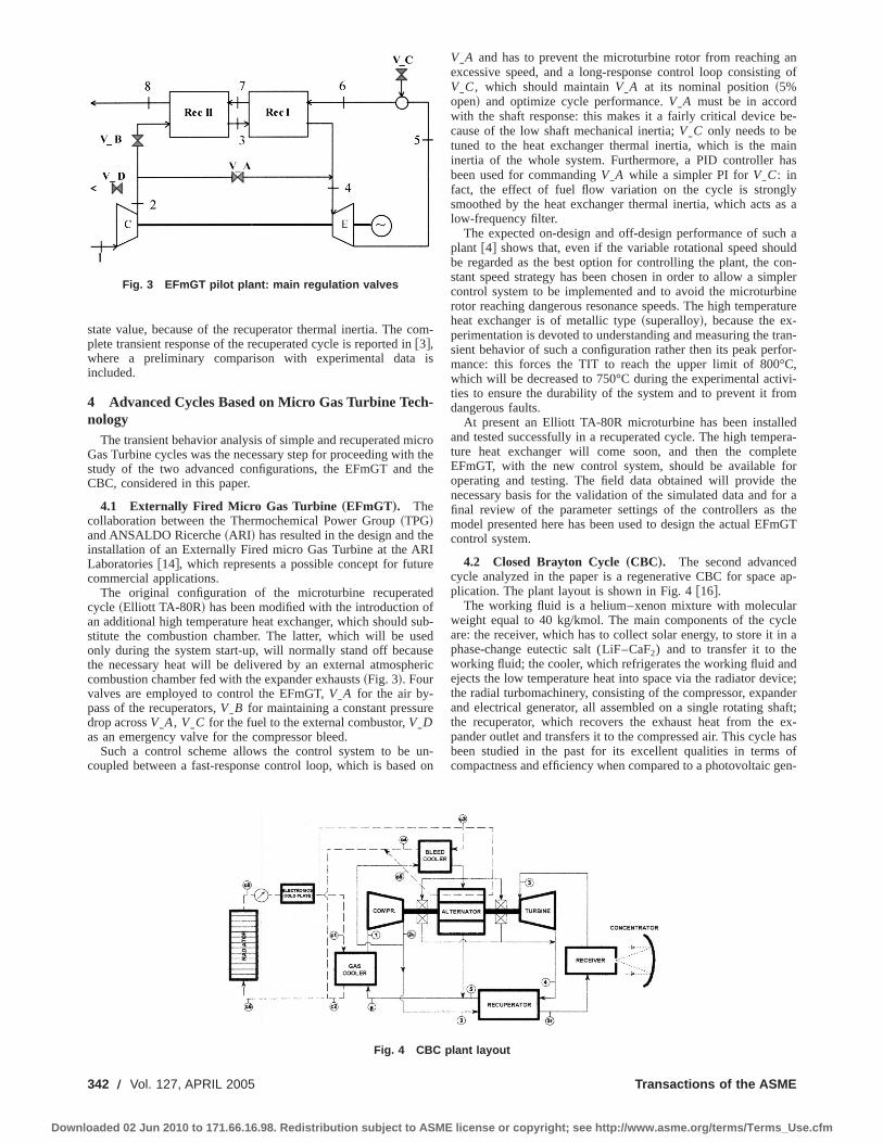
state value, because of the recuperator thermal inertia. The com-plete transient response of the recuperated cycle is reported in@3#,where a preliminary comparison with experimental data isincluded.

4 Advanced Cycles Based on Micro Gas Turbine Tech-nology

The transient behavior analysis of simple and recuperated microGas Turbine cycles was the necessary step for proceeding with thestudy of the two advanced configurations, the EFmGT and theCBC, considered in this paper.

4.1 Externally Fired Micro Gas Turbine „EFmGT…. Thecollaboration between the Thermochemical Power Group~TPG!and ANSALDO Ricerche~ARI! has resulted in the design and theinstallation of an Externally Fired micro Gas Turbine at the ARILaboratories@14#, which represents a possible concept for futurecommercial applications.

The original configuration of the microturbine recuperatedcycle ~Elliott TA-80R! has been modified with the introduction ofan additional high temperature heat exchanger, which should sub-stitute the combustion chamber. The latter, which will be usedonly during the system start-up, will normally stand off becausethe necessary heat will be delivered by an external atmosphericcombustion chamber fed with the expander exhausts~Fig. 3!. Fourvalves are employed to control the EFmGT,VIA for the air by-pass of the recuperators,VIB for maintaining a constant pressuredrop acrossVIA, VIC for the fuel to the external combustor,VIDas an emergency valve for the compressor bleed.

Such a control scheme allows the control system to be un-coupled between a fast-response control loop, which is based on

VIA and has to prevent the microturbine rotor from reaching anexcessive speed, and a long-response control loop consisting ofVIC, which should maintainVIA at its nominal position~5%open! and optimize cycle performance.VIA must be in accordwith the shaft response: this makes it a fairly critical device be-cause of the low shaft mechanical inertia;VIC only needs to betuned to the heat exchanger thermal inertia, which is the maininertia of the whole system. Furthermore, a PID controller hasbeen used for commandingVIA while a simpler PI forVIC: infact, the effect of fuel flow variation on the cycle is stronglysmoothed by the heat exchanger thermal inertia, which acts as alow-frequency filter.

The expected on-design and off-design performance of such aplant @4# shows that, even if the variable rotational speed shouldbe regarded as the best option for controlling the plant, the con-stant speed strategy has been chosen in order to allow a simplercontrol system to be implemented and to avoid the microturbinerotor reaching dangerous resonance speeds. The high temperatureheat exchanger is of metallic type~superalloy!, because the ex-perimentation is devoted to understanding and measuring the tran-sient behavior of such a configuration rather then its peak perfor-mance: this forces the TIT to reach the upper limit of 800°C,which will be decreased to 750°C during the experimental activi-ties to ensure the durability of the system and to prevent it fromdangerous faults.

At present an Elliott TA-80R microturbine has been installedand tested successfully in a recuperated cycle. The high tempera-ture heat exchanger will come soon, and then the completeEFmGT, with the new control system, should be available foroperating and testing. The field data obtained will provide thenecessary basis for the validation of the simulated data and for afinal review of the parameter settings of the controllers as themodel presented here has been used to design the actual EFmGTcontrol system.

4.2 Closed Brayton Cycle„CBC…. The second advancedcycle analyzed in the paper is a regenerative CBC for space ap-plication. The plant layout is shown in Fig. 4@16#.

The working fluid is a helium–xenon mixture with molecularweight equal to 40 kg/kmol. The main components of the cycleare: the receiver, which has to collect solar energy, to store it in aphase-change eutectic salt (LiF–CaF2) and to transfer it to theworking fluid; the cooler, which refrigerates the working fluid andejects the low temperature heat into space via the radiator device;the radial turbomachinery, consisting of the compressor, expanderand electrical generator, all assembled on a single rotating shaft;the recuperator, which recovers the exhaust heat from the ex-pander outlet and transfers it to the compressed air. This cycle hasbeen studied in the past for its excellent qualities in terms ofcompactness and efficiency when compared to a photovoltaic gen-

Fig. 3 EFmGT pilot plant: main regulation valves

Fig. 4 CBC plant layout



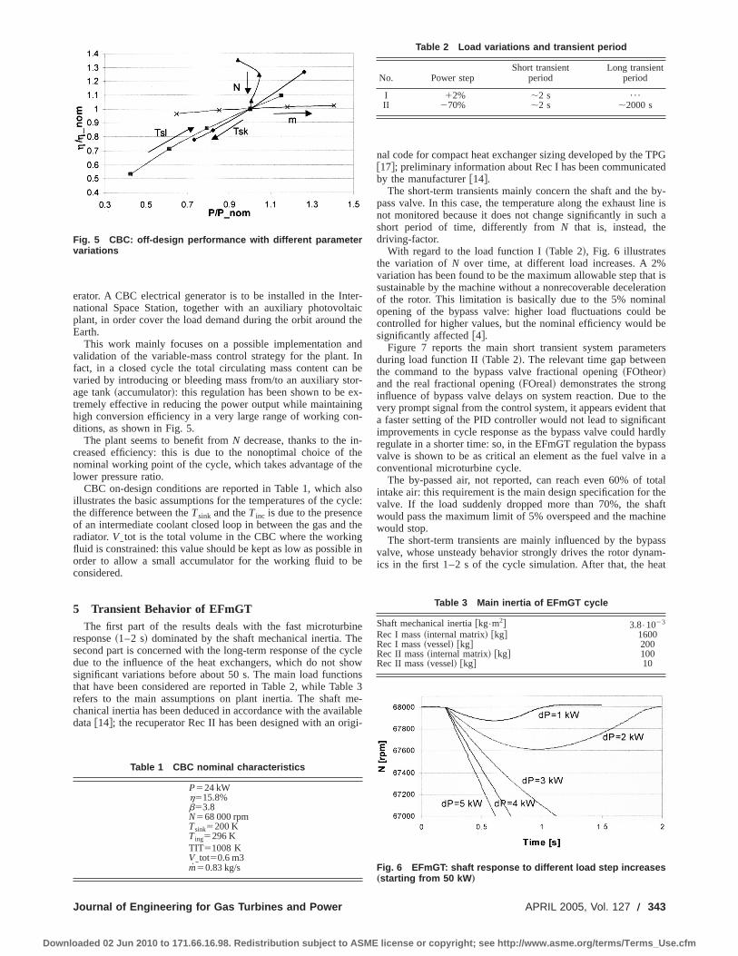
erator. A CBC electrical generator is to be installed in the Inter-national Space Station, together with an auxiliary photovoltaicplant, in order cover the load demand during the orbit around theEarth.

This work mainly focuses on a possible implementation andvalidation of the variable-mass control strategy for the plant. Infact, in a closed cycle the total circulating mass content can bevaried by introducing or bleeding mass from/to an auxiliary stor-age tank~accumulator!: this regulation has been shown to be ex-tremely effective in reducing the power output while maintaininghigh conversion efficiency in a very large range of working con-ditions, as shown in Fig. 5.

The plant seems to benefit fromN decrease, thanks to the in-creased efficiency: this is due to the nonoptimal choice of thenominal working point of the cycle, which takes advantage of thelower pressure ratio.

CBC on-design conditions are reported in Table 1, which alsoillustrates the basic assumptions for the temperatures of the cycle:the difference between theTsink and theTinc is due to the presenceof an intermediate coolant closed loop in between the gas and theradiator.VItot is the total volume in the CBC where the workingfluid is constrained: this value should be kept as low as possible inorder to allow a small accumulator for the working fluid to beconsidered.

5 Transient Behavior of EFmGTThe first part of the results deals with the fast microturbine

response~1–2 s! dominated by the shaft mechanical inertia. Thesecond part is concerned with the long-term response of the cycledue to the influence of the heat exchangers, which do not showsignificant variations before about 50 s. The main load functionsthat have been considered are reported in Table 2, while Table 3refers to the main assumptions on plant inertia. The shaft me-chanical inertia has been deduced in accordance with the availabledata@14#; the recuperator Rec II has been designed with an origi-

nal code for compact heat exchanger sizing developed by the TPG@17#; preliminary information about Rec I has been communicatedby the manufacturer@14#.

The short-term transients mainly concern the shaft and the by-pass valve. In this case, the temperature along the exhaust line isnot monitored because it does not change significantly in such ashort period of time, differently fromN that is, instead, thedriving-factor.

With regard to the load function I~Table 2!, Fig. 6 illustratesthe variation ofN over time, at different load increases. A 2%variation has been found to be the maximum allowable step that issustainable by the machine without a nonrecoverable decelerationof the rotor. This limitation is basically due to the 5% nominalopening of the bypass valve: higher load fluctuations could becontrolled for higher values, but the nominal efficiency would besignificantly affected@4#.

Figure 7 reports the main short transient system parametersduring load function II~Table 2!. The relevant time gap betweenthe command to the bypass valve fractional opening~FOtheor!and the real fractional opening~FOreal! demonstrates the stronginfluence of bypass valve delays on system reaction. Due to thevery prompt signal from the control system, it appears evident thata faster setting of the PID controller would not lead to significantimprovements in cycle response as the bypass valve could hardlyregulate in a shorter time: so, in the EFmGT regulation the bypassvalve is shown to be as critical an element as the fuel valve in aconventional microturbine cycle.

The by-passed air, not reported, can reach even 60% of totalintake air: this requirement is the main design specification for thevalve. If the load suddenly dropped more than 70%, the shaftwould pass the maximum limit of 5% overspeed and the machinewould stop.

The short-term transients are mainly influenced by the bypassvalve, whose unsteady behavior strongly drives the rotor dynam-ics in the first 1–2 s of the cycle simulation. After that, the heat

Fig. 5 CBC: off-design performance with different parametervariations

Table 1 CBC nominal characteristics

P524 kWh515.8%b53.8N568 000 rpmTsink5200 KTing5296 KTIT51008 KVItot50.6 m3m50.83 kg/s

Table 2 Load variations and transient period

No. Power stepShort transient

periodLong transient

period

I 12% ;2 s ¯

II 270% ;2 s ;2000 s

Table 3 Main inertia of EFmGT cycle

Shaft mechanical inertia@kg•m2# 3.8•1023

Rec I mass~internal matrix! @kg# 1600Rec I mass~vessel! @kg# 200Rec II mass~internal matrix! @kg# 100Rec II mass~vessel! @kg# 10

Fig. 6 EFmGT: shaft response to different load step increases„starting from 50 kW …



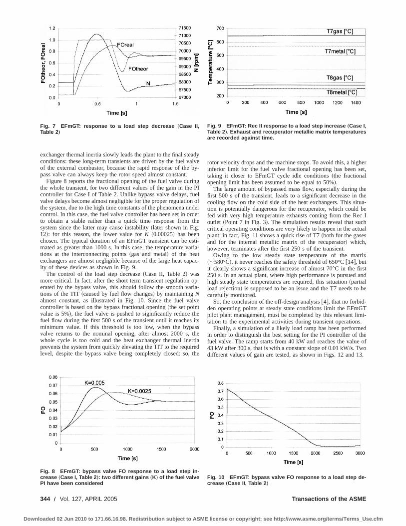
exchanger thermal inertia slowly leads the plant to the final steadyconditions: these long-term transients are driven by the fuel valveof the external combustor, because the rapid response of the by-pass valve can always keep the rotor speed almost constant.

Figure 8 reports the fractional opening of the fuel valve duringthe whole transient, for two different values of the gain in the PIcontroller for Case I of Table 2. Unlike bypass valve delays, fuelvalve delays become almost negligible for the proper regulation ofthe system, due to the high time constants of the phenomena undercontrol. In this case, the fuel valve controller has been set in orderto obtain a stable rather than a quick time response from thesystem since the latter may cause instability~later shown in Fig.12!: for this reason, the lower value forK ~0.00025! has beenchosen. The typical duration of an EFmGT transient can be esti-mated as greater than 1000 s. In this case, the temperature varia-tions at the interconnecting points~gas and metal! of the heatexchangers are almost negligible because of the large heat capac-ity of these devices as shown in Fig. 9.

The control of the load step decrease~Case II, Table 2! wasmore critical. In fact, after the short-term transient regulation op-erated by the bypass valve, this should follow the smooth varia-tions of the TIT~caused by fuel flow changes! by maintainingNalmost constant, as illustrated in Fig. 10. Since the fuel valvecontroller is based on the bypass fractional opening~the set pointvalue is 5%!, the fuel valve is pushed to significantly reduce thefuel flow during the first 500 s of the transient until it reaches itsminimum value. If this threshold is too low, when the bypassvalve returns to the nominal opening, after almost 2000 s, thewhole cycle is too cold and the heat exchanger thermal inertiaprevents the system from quickly elevating the TIT to the requiredlevel, despite the bypass valve being completely closed: so, the

rotor velocity drops and the machine stops. To avoid this, a higherinferior limit for the fuel valve fractional opening has been set,taking it closer to EFmGT cycle idle conditions~the fractionalopening limit has been assumed to be equal to 50%!.

The large amount of bypassed mass flow, especially during thefirst 500 s of the transient, leads to a significant decrease in thecooling flow on the cold side of the heat exchangers. This situa-tion is potentially dangerous for the recuperator, which could befed with very high temperature exhausts coming from the Rec Ioutlet ~Point 7 in Fig. 3!. The simulation results reveal that suchcritical operating conditions are very likely to happen in the actualplant: in fact, Fig. 11 shows a quick rise of T7~both for the gasesand for the internal metallic matrix of the recuperator! which,however, terminates after the first 250 s of the transient.

Owing to the low steady state temperature of the matrix~;580°C!, it never reaches the safety threshold of 650°C@14#, butit clearly shows a significant increase of almost 70°C in the first250 s. In an actual plant, where high performance is pursued andhigh steady state temperatures are required, this situation~partialload rejection! is supposed to be an issue and the T7 needs to becarefully monitored.

So, the conclusion of the off-design analysis@4#, that no forbid-den operating points at steady state conditions limit the EFmGTpilot plant management, must be completed by this relevant limi-tation to the experimental activities during transient operations.

Finally, a simulation of a likely load ramp has been performedin order to distinguish the best setting for the PI controller of thefuel valve. The ramp starts from 40 kW and reaches the value of43 kW after 300 s, that is with a constant slope of 0.01 kW/s. Twodifferent values of gain are tested, as shown in Figs. 12 and 13.

Fig. 7 EFmGT: response to a load step decrease „Case II,Table 2 …

Fig. 8 EFmGT: bypass valve FO response to a load step in-crease „Case I, Table 2 …: two different gains „K… of the fuel valvePI have been considered

Fig. 9 EFmGT: Rec II response to a load step increase „Case I,Table 2 …. Exhaust and recuperator metallic matrix temperaturesare recorded against time.

Fig. 10 EFmGT: bypass valve FO response to a load step de-crease „Case II, Table 2 …



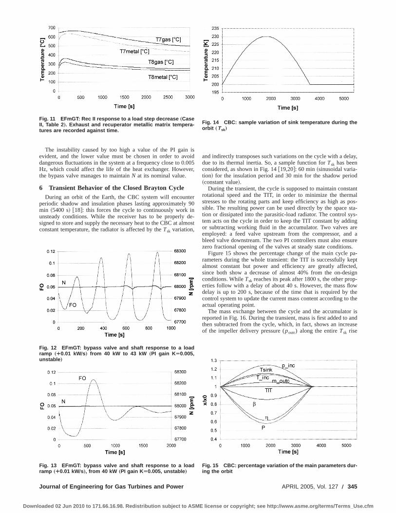
The instability caused by too high a value of the PI gain isevident, and the lower value must be chosen in order to avoiddangerous fluctuations in the system at a frequency close to 0.005Hz, which could affect the life of the heat exchanger. However,the bypass valve manages to maintainN at its nominal value.

6 Transient Behavior of the Closed Brayton CycleDuring an orbit of the Earth, the CBC system will encounter

periodic shadow and insulation phases lasting approximately 90min ~5400 s! @18#: this forces the cycle to continuously work inunsteady conditions. While the receiver has to be properly de-signed to store and supply the necessary heat to the CBC at almostconstant temperature, the radiator is affected by theTsk variation,

and indirectly transposes such variations on the cycle with a delay,due to its thermal inertia. So, a sample function forTsk has beenconsidered, as shown in Fig. 14@19,20#: 60 min ~sinusoidal varia-tion! for the insulation period and 30 min for the shadow period~constant value!.

During the transient, the cycle is supposed to maintain constantrotational speed and the TIT, in order to minimize the thermalstresses to the rotating parts and keep efficiency as high as pos-sible. The resulting power can be used directly by the space sta-tion or dissipated into the parasitic-load radiator. The control sys-tem acts on the cycle in order to keep the TIT constant by addingor subtracting working fluid in the accumulator. Two valves areemployed: a feed valve upstream from the compressor, and ableed valve downstream. The two PI controllers must also ensurezero fractional opening of the valves at steady state conditions.

Figure 15 shows the percentage change of the main cycle pa-rameters during the whole transient: the TIT is successfully keptalmost constant but power and efficiency are greatly affected,since both show a decrease of almost 40% from the on-designconditions. WhileTsk reaches its peak after 1800 s, the other prop-erties follow with a delay of about 40 s. However, the mass flowdelay is up to 200 s, because of the time that is required by thecontrol system to update the current mass content according to theactual operating point.

The mass exchange between the cycle and the accumulator isreported in Fig. 16. During the transient, mass is first added to andthen subtracted from the cycle, which, in fact, shows an increaseof the impeller delivery pressure (poutc) along the entireTsk rise

Fig. 11 EFmGT: Rec II response to a load step decrease „CaseII, Table 2 …. Exhaust and recuperator metallic matrix tempera-tures are recorded against time.

Fig. 12 EFmGT: bypass valve and shaft response to a loadramp „¿0.01 kWÕs… from 40 kW to 43 kW „PI gain K Ä0.005,unstable …

Fig. 13 EFmGT: bypass valve and shaft response to a loadramp „¿0.01 kWÕs…, from 40 kW „PI gain K Ä0.005, unstable …

Fig. 14 CBC: sample variation of sink temperature during theorbit „Tsk…

Fig. 15 CBC: percentage variation of the main parameters dur-ing the orbit



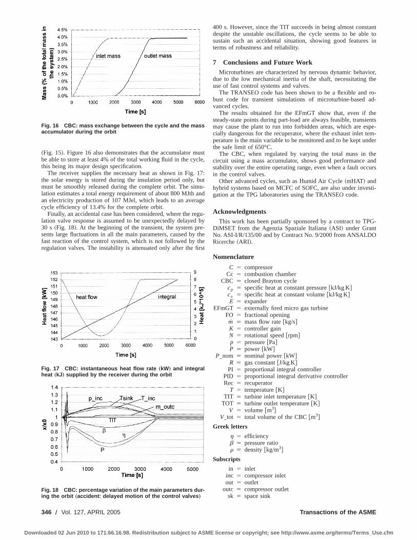
~Fig. 15!. Figure 16 also demonstrates that the accumulator mustbe able to store at least 4% of the total working fluid in the cycle,this being its major design specification.

The receiver supplies the necessary heat as shown in Fig. 17:the solar energy is stored during the insulation period only, butmust be smoothly released during the complete orbit. The simu-lation estimates a total energy requirement of about 800 MJth andan electricity production of 107 MJel, which leads to an averagecycle efficiency of 13.4% for the complete orbit.

Finally, an accidental case has been considered, where the regu-lation valve response is assumed to be unexpectedly delayed by30 s ~Fig. 18!. At the beginning of the transient, the system pre-sents large fluctuations in all the main parameters, caused by thefast reaction of the control system, which is not followed by theregulation valves. The instability is attenuated only after the first

400 s. However, since the TIT succeeds in being almost constantdespite the unstable oscillations, the cycle seems to be able tosustain such an accidental situation, showing good features interms of robustness and reliability.

7 Conclusions and Future WorkMicroturbines are characterized by nervous dynamic behavior,

due to the low mechanical inertia of the shaft, necessitating theuse of fast control systems and valves.

The TRANSEO code has been shown to be a flexible and ro-bust code for transient simulations of microturbine-based ad-vanced cycles.

The results obtained for the EFmGT show that, even if thesteady-state points during part-load are always feasible, transientsmay cause the plant to run into forbidden areas, which are espe-cially dangerous for the recuperator, where the exhaust inlet tem-perature is the main variable to be monitored and to be kept underthe safe limit of 650°C.

The CBC, when regulated by varying the total mass in thecircuit using a mass accumulator, shows good performance andstability over the entire operating range, even when a fault occursin the control valves.

Other advanced cycles, such as Humid Air Cycle~mHAT! andhybrid systems based on MCFC of SOFC, are also under investi-gation at the TPG laboratories using the TRANSEO code.

AcknowledgmentsThis work has been partially sponsored by a contract to TPG-

DiMSET from the Agenzia Spaziale Italiana~ASI! under GrantNo. ASI-I/R/135/00 and by Contract No. 9/2000 from ANSALDORicerche~ARI!.

Nomenclature

C 5 compressorCc 5 combustion chamber

CBC 5 closed Brayton cyclecp 5 specific heat at constant pressure@kJ/kg K#cv 5 specific heat at constant volume@kJ/kg K#E 5 expander

EFmGT 5 externally fired micro gas turbineFO 5 fractional openingm 5 mass flow rate@kg/s#K 5 controller gainN 5 rotational speed@rpm#p 5 pressure@Pa#P 5 power @kW#

PInom 5 nominal power@kW#R 5 gas constant@J/kg K#PI 5 proportional integral controller

PID 5 proportional integral derivative controllerRec 5 recuperator

T 5 temperature@K#TIT 5 turbine inlet temperature@K#

TOT 5 turbine outlet temperature@K#V 5 volume @m3#

VItot 5 total volume of the CBC@m3#

Greek letters

h 5 efficiencyb 5 pressure ratior 5 density@kg/m3#

Subscripts

in 5 inletinc 5 compressor inletout 5 outlet

outc 5 compressor outletsk 5 space sink

Fig. 16 CBC: mass exchange between the cycle and the massaccumulator during the orbit

Fig. 17 CBC: instantaneous heat flow rate „kW… and integralheat „kJ … supplied by the receiver during the orbit

Fig. 18 CBC: percentage variation of the main parameters dur-ing the orbit „accident: delayed motion of the control valves …



sl 5 saltt 5 total

References@1# Rodgers, C., ‘‘Microturbine Cycle Options,’’ ASME paper No. 2001-GT-0552.@2# Rowen, W. I., 1992, ‘‘Simplified Mathematical Representation of Single Shaft

Gas Turbines in Mechanical Drive Service,’’ Turbomachinery Inter.,33, pp.26–32.

@3# Cerelli, E., ‘‘Theoretical Modelling and Experimental Measurements of Micro-turbine Cycles for Distributed Trigeneration,’’ 2002, Master thesis, TPG-DiMSET, Universitadi Genova, Italy.

@4# Traverso, A., Magistri, L., Scarpellini, R., and Massardo, A. F., ‘‘Demonstra-tion Plant and Expected Performance of An Externally Fired Micro Gas Tur-bine for Distributed Power Generation,’’ ASME Paper No. 2003-GT-38268.

@5# Agazzani, A., and Massardo, A., 1995, ‘‘Advanced Solar Dynamic SpacePower Systems, Part I: Efficiency and Surface Optimization,’’ ASME Trans. J.Solar Energy Eng.,117, pp. 265–273.

@6# Agazzani, A., and Massardo, A., 1995, ‘‘Advanced Solar Dynamic SpacePower Systems; Part II: Detailed Design and Specific Parameters Optimiza-tion,’’ ASME Trans. J. Solar Energy Eng.,117, pp. 273–281.

@7# Massardo, A. F., Tagliafico, L. A., Fossa, M., and Agazzani, A., 1997, ‘‘SolarSpace Power System Optimization With Ultralight Radiator,’’ J. Propul.Power,13, pp. 560–564.

@8# Parente, J., Traverso, A., and Massardo, A. F., ‘‘Micro Humid Air Cycle. PartA: Thermodynamic and Technical Aspects,’’ ASME Paper 2003-GT-38326.

@9# Magistri, L., Bozzo, R., Costamagna, P., and Massardo, A. F., ‘‘SimplifiedVersus Detailed SOFC Reactor Models and Influence on the Simulation of theDesign Point Performance of Hybrid Systems,’’ ASME Paper 2002-GT-30653.

@10# Schobeiri, M. T., Attia, M., and Lippe, C., 1994, ‘‘GETRAN: A Generic,

Modularly Structured Computer Code for Simulation of Dynamic Behavior ofAero- and Power Generation Gas Turbine Engines,’’ J. Eng. Gas TurbinesPower,116, pp. 483–494.

@11# Crosa, G., Fantini, L., Ferrari, G., Pizzimenti, L., and Trucco, A., ‘‘SteadyState and Dynamic Behavior of an Indirect Fired Gas Turbine Plant,’’ ASMEpaper 98-GT-167.

@12# Pilidis, P., and Maccallum, N. R. L., ‘‘A General Program for the Prediction ofthe Transient Performance of Gas Turbines,’’ 1985, ASME Paper 85-GT-265.

@13# Calzolari, F., ‘‘Transient Behavior and Control System for Advanced CyclesBased on Micro Gas Turbine Technology,’’ 2002, Master thesis, TPG-DiMSET, Universitadi Genova, Italy.

@14# ‘‘Externally Fired Micro Gas Turbine for Distributed Power Generation,’’2002, ANSALDO Ricerche, Research Contract No. 9/2000, Final Report.

@15# White, F. M., 1994,Fluid Mechanics, 3rd ed., McGraw–Hill, New York, pp.335–341.

@16# Korakianitis, T., Hochstein, J. I., and Zou, D., ‘‘Prediction of Transient Ther-modynamic Response of a Closed-Cycle Regenerative Gas Turbine,’’ ASMEPaper 93-GT-136.

@17# Rio, R., 2001, ‘‘Regenerated Microturbines for Distribuited Power Generation:Thermoeconomic Assessment,’’ Master thesis, TPG-DIMSET, Universita` diGenova, Genova, Italy.

@18# ‘‘Closed Brayton Cycle for Space Applications: Off-Dedign and TransientAnalysis,’’ Agenzia Spaziale Italiana~ASI!, Grant No. ASI-I/R/135/00, FinalReport.

@19# Bons, R., Hanlon, J., and Spencer, S., 1988, ‘‘Predicting the Behavior of SolarDynamic Closed Brayton Cycle Power Conversion Systems,’’ ASME Trans. J.Eng. Gas Turbines and Power,110, pp. 636–640.

@20# Harper William, B., Boyle, Jr., Robert V., and Kudija, Charles T., 1990, ‘‘SolarDynamic CBC Power for Space Station Freedom,’’ ASME Paper 90-GT-70.



Francesco FantozziDipartimento di Ingegneria Industriale,

Universita degli Studi di Perugia,Via G. Duranti 1A/4,06125 Perugia, Italy


Bruno D’AlessandroIngegneria dei Materiali,

Universita degli Studi di Perugia,Loc. Pentima Bassa 21,

05100 Terni, Italye-mail: [email protected]

Umberto DesideriDipartimento di Ingegneria Industriale,

Universita degli Studi di Perugia,Via G. Duranti 1A/4,06125 Perugia, Italy


Integrated Pyrolysis RegeneratedPlant (IPRP): An Efficient andScalable Concept for Gas TurbineBased Energy Conversion FromBiomass and WasteA massive effort towards sustainability is necessary to prevent global warming and energysources impoverishment: both biomass and waste to energy conversion may represent keyactions to reach this goal. At the present, state of the art available technologies forbiomass and waste to energy conversion are similar and include low to mid efficiencygrate incineration or fluidized bed combustion with steam power cycles or mid to highefficiency gas turbine based cycles through integrated gasification technology. Neverthe-less, these plants are all available from mid-to-high scale range that can be highly intru-sive on protected areas and socially unacceptable. This paper proposes an innovative, lowcost, high efficiency plant in which the residue is gasified in the absence of oxygen(pyrolysis), in a rotary kiln, by means of a highly regenerative gas turbine based cycle.Pyrolysis is preferred to gasification, because the syngas obtained has a higher lowheating value and produces char or tar as a by-product with an interesting energy contentto be re-utilized inside the cycle. Different plant configurations are proposed and dis-cussed through principal thermodynamic variables parametric analysis. Results show thatvery interesting efficiencies are obtainable in the 30–40% range for every plant scale.This fact shows how IPRP technology can provide an interesting alternative to traditionaltechnologies, especially for the small size (below 5MW). Moreover, the IPRP technologyprovides a unique solution for microscale (below 500 kW) power plants, opening a newand competitive possibility for distributed biomass or waste to energy conversion systemswhere low environmental and social impact turns into higher interest and positive dis-semination effect.@DOI: 10.1115/1.1789513#

1 IntroductionThe energy conversion of biomass and/or waste~B&W ! is ad-

dressed as one of the key issues to reach sustainability and to meetthe goals of the Kyoto Protocol@1#. The best available technologyfor B&W electric energy conversion is still the grate-based incin-eration with a net electric efficiency lower than 30% and a mini-mum plant size for economical feasibility above 2 MWe. Higherefficiencies may be obtained through an intermediate conversion~gasification, anaerobic digestion! that turns B&W into a medium-low calorific fuel gas that can be used in a high efficiency cyclebased on internal combustion engine~ICE! or gas turbine~GT!but still at a demonstrative stage. Nevertheless, the higher capitalcost and the more complicated arrangement of these plants main-tains the minimum size for economical feasibility still on the me-dium to high scale, as briefly summarized in Table 1. This turnsinto relative big plants and B&W supply chain that may be con-sidered intrusive for protective areas and socially unacceptable.For small to micro scale conversion, externally fired cycles arepromising but still at a demonstration level due to material prob-lems for hot air heat exchangers technology@4,5#.

B&W energy conversion is therefore hampered because:• it is feasible on medium to big scale that is often considered

intrusive and socially unacceptable;

• there are no technologies available for the small–micro scalethat benefits of the intrinsic distributed nature of B&W.

This paper analyzes the integrated pyrolysis regenerated plant~IPRP!, a new concept for B&W energy conversion, that putstogether both high performance and plant simplicity and it is alsoscalable even to the micro scale. The plant is based on an inter-mediate conversion of B&W to a medium-high LHV gas throughpyrolysis ~a well-known process@6–13#! in a rotary kiln reactor.The syngas obtained fuels a GT and the exhaust gases from theGT are fed back to the reactor providing the energy required tomaintain the pyrolysis process. If necessary it is possible to in-crease the enthalpy content of the GT exhaust gases through com-bustion of the residual tar/char produced by pyrolysis. With refer-ence to other pyrolysis based combined cycle@14# the IPRPtechnology is simpler and more economic because it does notrequire a bottoming steam cycle.

2 Plant DescriptionFigure 1 shows the plant layout analyzed in the present work.

The rotary-kiln pyrolyzer~PYRO! is fed by the generic residualfuel ~RF! through a hopper. The rotary-kiln pyrolyzer is built as atube in tube heat exchanger where the inner cylinder representsthe pyrolysis reaction chamber where the RF degrades to syngas,tar and char in absence of oxygen. The hollow space between thetwo cylinders is the flow path for the hot gases exhausted from theGT, which provide the heat necessary to pyrolyze the RF. Exhaustgases from the pyrolyzer may be used to preheat GT primary airin a recuperator~REC, when present!, before being conveyed tothe filtering section and to the stack. Syngas obtained from py-rolysis




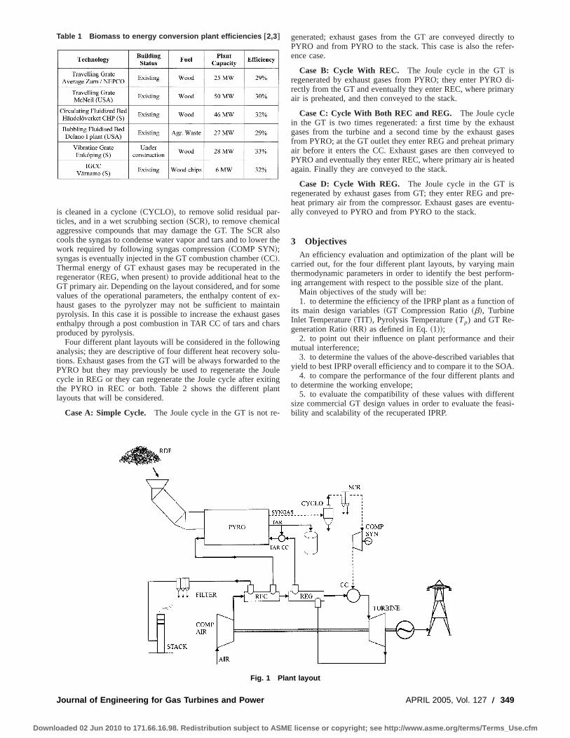
is cleaned in a cyclone~CYCLO!, to remove solid residual par-ticles, and in a wet scrubbing section~SCR!, to remove chemicalaggressive compounds that may damage the GT. The SCR alsocools the syngas to condense water vapor and tars and to lower thework required by following syngas compression~COMP SYN!;syngas is eventually injected in the GT combustion chamber~CC!.Thermal energy of GT exhaust gases may be recuperated in theregenerator~REG, when present! to provide additional heat to theGT primary air. Depending on the layout considered, and for somevalues of the operational parameters, the enthalpy content of ex-haust gases to the pyrolyzer may not be sufficient to maintainpyrolysis. In this case it is possible to increase the exhaust gasesenthalpy through a post combustion in TAR CC of tars and charsproduced by pyrolysis.

Four different plant layouts will be considered in the followinganalysis; they are descriptive of four different heat recovery solu-tions. Exhaust gases from the GT will be always forwarded to thePYRO but they may previously be used to regenerate the Joulecycle in REG or they can regenerate the Joule cycle after exitingthe PYRO in REC or both. Table 2 shows the different plantlayouts that will be considered.

Case A: Simple Cycle. The Joule cycle in the GT is not re-

generated; exhaust gases from the GT are conveyed directly toPYRO and from PYRO to the stack. This case is also the refer-ence case.

Case B: Cycle With REC. The Joule cycle in the GT isregenerated by exhaust gases from PYRO; they enter PYRO di-rectly from the GT and eventually they enter REC, where primaryair is preheated, and then conveyed to the stack.

Case C: Cycle With Both REC and REG. The Joule cyclein the GT is two times regenerated: a first time by the exhaustgases from the turbine and a second time by the exhaust gasesfrom PYRO; at the GT outlet they enter REG and preheat primaryair before it enters the CC. Exhaust gases are then conveyed toPYRO and eventually they enter REC, where primary air is heatedagain. Finally they are conveyed to the stack.

Case D: Cycle With REG. The Joule cycle in the GT isregenerated by exhaust gases from GT; they enter REG and pre-heat primary air from the compressor. Exhaust gases are eventu-ally conveyed to PYRO and from PYRO to the stack.

3 ObjectivesAn efficiency evaluation and optimization of the plant will be

carried out, for the four different plant layouts, by varying mainthermodynamic parameters in order to identify the best perform-ing arrangement with respect to the possible size of the plant.

Main objectives of the study will be:1. to determine the efficiency of the IPRP plant as a function of

its main design variables~GT Compression Ratio~b!, TurbineInlet Temperature~TIT!, Pyrolysis Temperature (Tp) and GT Re-generation Ratio~RR! as defined in Eq.~1!!;

2. to point out their influence on plant performance and theirmutual interference;

3. to determine the values of the above-described variables thatyield to best IPRP overall efficiency and to compare it to the SOA.

4. to compare the performance of the four different plants andto determine the working envelope;

5. to evaluate the compatibility of these values with differentsize commercial GT design values in order to evaluate the feasi-bility and scalability of the recuperated IPRP.

Table 1 Biomass to energy conversion plant efficiencies †2,3‡

Fig. 1 Plant layout



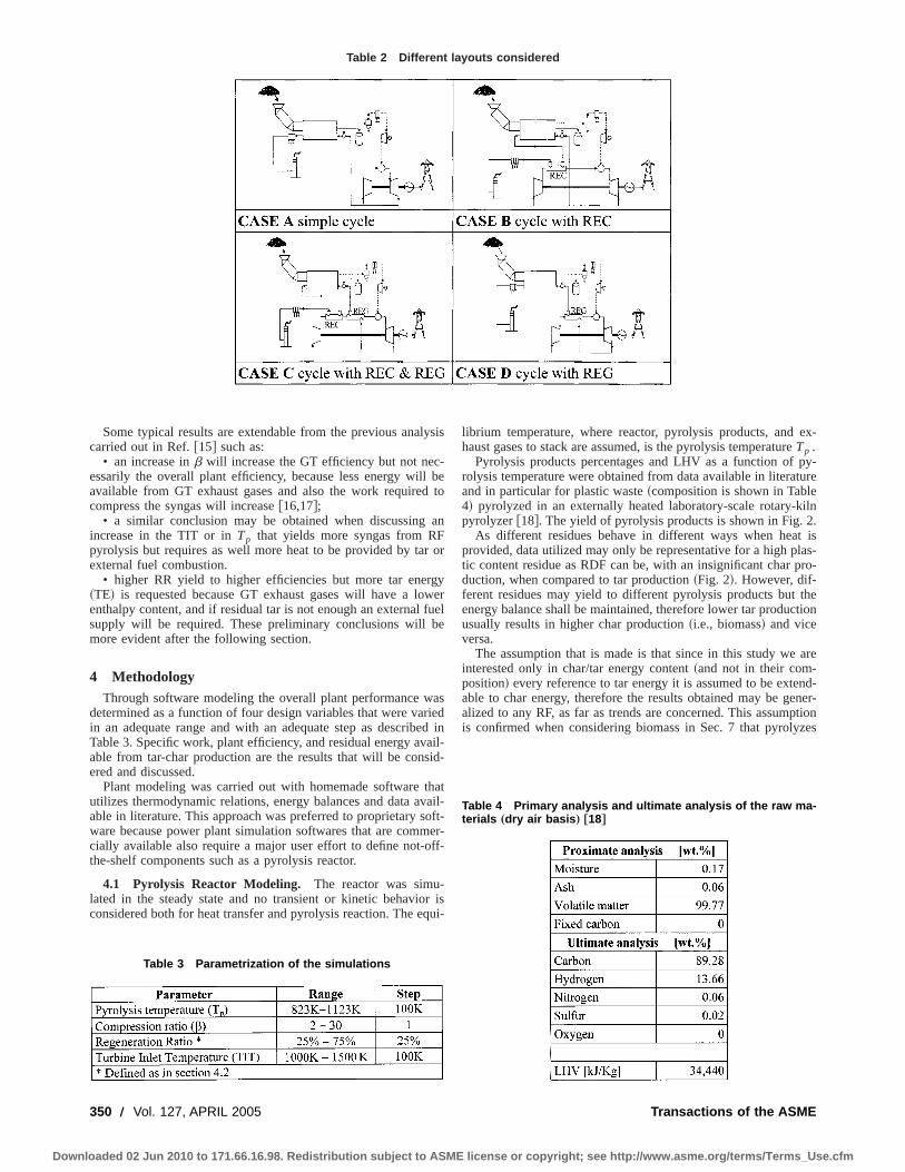
Some typical results are extendable from the previous analysiscarried out in Ref.@15# such as:

• an increase inb will increase the GT efficiency but not nec-essarily the overall plant efficiency, because less energy will beavailable from GT exhaust gases and also the work required tocompress the syngas will increase@16,17#;

• a similar conclusion may be obtained when discussing anincrease in the TIT or inTp that yields more syngas from RFpyrolysis but requires as well more heat to be provided by tar orexternal fuel combustion.

• higher RR yield to higher efficiencies but more tar energy~TE! is requested because GT exhaust gases will have a lowerenthalpy content, and if residual tar is not enough an external fuelsupply will be required. These preliminary conclusions will bemore evident after the following section.

4 MethodologyThrough software modeling the overall plant performance was

determined as a function of four design variables that were variedin an adequate range and with an adequate step as described inTable 3. Specific work, plant efficiency, and residual energy avail-able from tar-char production are the results that will be consid-ered and discussed.

Plant modeling was carried out with homemade software thatutilizes thermodynamic relations, energy balances and data avail-able in literature. This approach was preferred to proprietary soft-ware because power plant simulation softwares that are commer-cially available also require a major user effort to define not-off-the-shelf components such as a pyrolysis reactor.

4.1 Pyrolysis Reactor Modeling. The reactor was simu-lated in the steady state and no transient or kinetic behavior isconsidered both for heat transfer and pyrolysis reaction. The equi-

librium temperature, where reactor, pyrolysis products, and ex-haust gases to stack are assumed, is the pyrolysis temperatureTp .

Pyrolysis products percentages and LHV as a function of py-rolysis temperature were obtained from data available in literatureand in particular for plastic waste~composition is shown in Table4! pyrolyzed in an externally heated laboratory-scale rotary-kilnpyrolyzer@18#. The yield of pyrolysis products is shown in Fig. 2.

As different residues behave in different ways when heat isprovided, data utilized may only be representative for a high plas-tic content residue as RDF can be, with an insignificant char pro-duction, when compared to tar production~Fig. 2!. However, dif-ferent residues may yield to different pyrolysis products but theenergy balance shall be maintained, therefore lower tar productionusually results in higher char production~i.e., biomass! and viceversa.

The assumption that is made is that since in this study we areinterested only in char/tar energy content~and not in their com-position! every reference to tar energy it is assumed to be extend-able to char energy, therefore the results obtained may be gener-alized to any RF, as far as trends are concerned. This assumptionis confirmed when considering biomass in Sec. 7 that pyrolyzes

Table 2 Different layouts considered

Table 3 Parametrization of the simulations

Table 4 Primary analysis and ultimate analysis of the raw ma-terials „dry air basis … †18‡



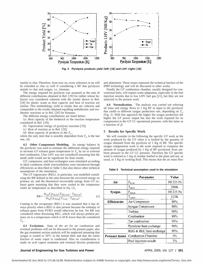
mainly to char. Therefore, from now on, every reference to tar willbe extended to char as well if considering a RF that pyrolyzesmainly to char and syngas, i.e., biomass.

The energy required for pyrolysis was assumed as the sum ofdifferent contributions obtained in Ref.@19# for rubber whose be-havior was considered coherent with the results shown in Ref.@18# for plastic waste as heat capacity and heat of reaction aresimilar. This methodology yield to results that are coherent andcomparable to the results obtained equalling endothermic and eso-thermic reactions as in Ref.@20# for biomass.

The different energy contributions are listed below:~a! Heat capacity of the feedstock to the reaction temperature

considered in Ref.@19#;~b! Vaporization energy of pyrolysis reactants@19#;~c! Heat of reaction as in Ref.@19#;~d! Heat capacity of products to theTp ,

where the only item that is sensibly dependent fromTp is the lastone,~d!.

4.2 Other Components Modeling. An energy balance inthe pyrolyzer was used to estimate the additional energy requiredto increase GT exhaust gases temperature toTp by tar or externalfuel combustion. Char LHV was not considered assuming that thesmall yield would not be significant for final results.

GT, compressor, and heat exchangers were simulated accordingto ideal conditions while irreversibilities were introduced throughefficiencies as described in Table 5 that also shows other technicalassumptions of the simulation.

The GT regenerator~REG!, in particular, was modelled consid-ering the RR defined as the ratio between the recovered energy onprimary air, and the theoretical recoverable energy from GT ex-haust gases assuming that they were cooled to the compressoroutlet air temperature as described in Eq.~1!,

RR5mAirCpAV,Air ~TREG,Out2TREG,In!

mEgCpAV,Eg~TT,Out2TREG,In!. (1)

Coming to the recuperator~REC! it was assumed that it has al-ways priority when a REG is also present because the enthalpy ofexhaust gases from PYRO would otherwise be lost. No RR wasconsidered when discussing REC, which will always preheat pri-mary air to a temperature which is 50 K lower than the consideredTp .

4.3 Exclusions. State of the art for tar combustion andeventual problems will not be discussed in the present paper; alsothe gas treatment section analysis will be neglected assuming thatsyngas is cooled to 50°C in the humid filter and that the entirefraction of water vapor is condensed. Also no consideration ismade on acid vapors treatment and eventual dioxins production

and abatement. These issues represent the technical barriers of theIPRP technology and will be discussed in other works.

Finally the GT combustion chamber, usually designed for con-ventional fuels, will require some adaptation, especially in the fuelinjection nozzles due to low LHV fuel gas@21#, but they are notanalyzed in the present work.

4.4 Normalization. The analysis was carried out referringall mass and energy flows to 1 Kg RF in input to the pyrolyzerthat yields to different syngas production rate, depending onTp~Fig. 2!. With this approach the higher the syngas production thehigher the GT power output but also the work required for itscompression to the GT CC operational pressure, with this latter asa function ofb.

5 Results for Specific WorkWe will consider in the following the specific GT work as the

work produced by the GT when it is fuelled by the quantity ofsyngas obtained from the pyrolysis of 1 Kg of RF. The specificsyngas compression work is the work required to compress theamount of syngas produced by 1 Kg of RF pyrolyzed, from am-bient pressure to the GT CC pressure. Therefore the GT specificwork is referred to 1 Kg of residue fuelled to the plant and not, asusual, to 1 Kg of working fluid. This means that the air mass flow

Fig. 2 Pyrolysis products yield „left … †18‡ and LHV „right … †18‡

Table 5 Technical assumption used in the simulation



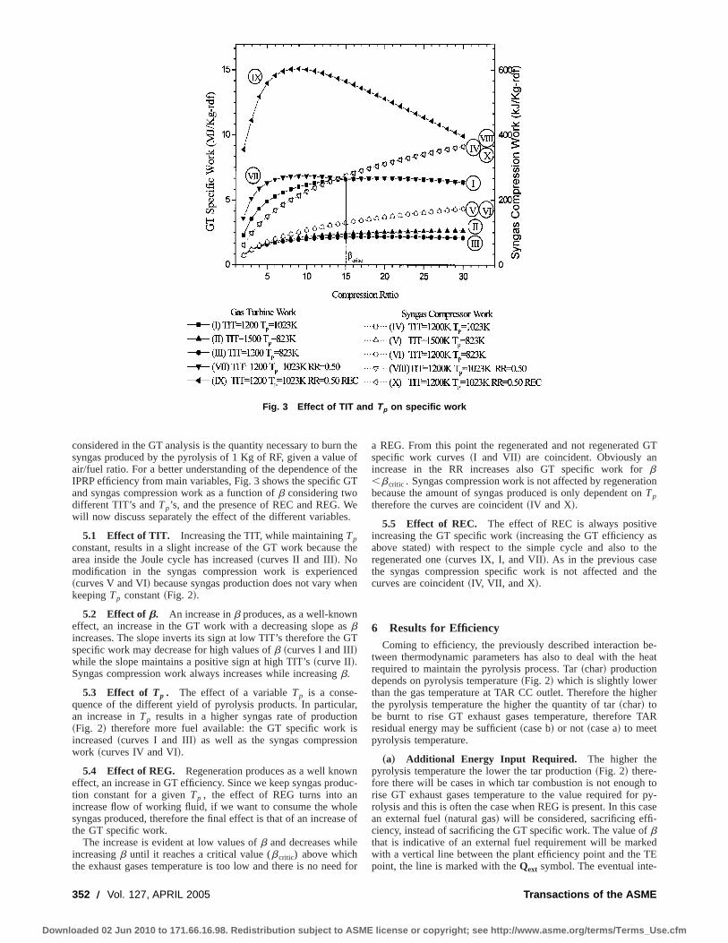
considered in the GT analysis is the quantity necessary to burn thesyngas produced by the pyrolysis of 1 Kg of RF, given a value ofair/fuel ratio. For a better understanding of the dependence of theIPRP efficiency from main variables, Fig. 3 shows the specific GTand syngas compression work as a function ofb considering twodifferent TIT’s andTp’s, and the presence of REC and REG. Wewill now discuss separately the effect of the different variables.

5.1 Effect of TIT. Increasing the TIT, while maintainingTpconstant, results in a slight increase of the GT work because thearea inside the Joule cycle has increased~curves II and III!. Nomodification in the syngas compression work is experienced~curves V and VI! because syngas production does not vary whenkeepingTp constant~Fig. 2!.

5.2 Effect ofb. An increase inb produces, as a well-knowneffect, an increase in the GT work with a decreasing slope asbincreases. The slope inverts its sign at low TIT’s therefore the GTspecific work may decrease for high values ofb ~curves I and III!while the slope maintains a positive sign at high TIT’s~curve II!.Syngas compression work always increases while increasingb.

5.3 Effect of Tp . The effect of a variableTp is a conse-quence of the different yield of pyrolysis products. In particular,an increase inTp results in a higher syngas rate of production~Fig. 2! therefore more fuel available: the GT specific work isincreased~curves I and III! as well as the syngas compressionwork ~curves IV and VI!.

5.4 Effect of REG. Regeneration produces as a well knowneffect, an increase in GT efficiency. Since we keep syngas produc-tion constant for a givenTp , the effect of REG turns into anincrease flow of working fluid, if we want to consume the wholesyngas produced, therefore the final effect is that of an increase ofthe GT specific work.

The increase is evident at low values ofb and decreases whileincreasingb until it reaches a critical value (bcritic) above whichthe exhaust gases temperature is too low and there is no need for

a REG. From this point the regenerated and not regenerated GTspecific work curves~I and VII! are coincident. Obviously anincrease in the RR increases also GT specific work forb,bcritic . Syngas compression work is not affected by regenerationbecause the amount of syngas produced is only dependent onTptherefore the curves are coincident~IV and X!.

5.5 Effect of REC. The effect of REC is always positiveincreasing the GT specific work~increasing the GT efficiency asabove stated! with respect to the simple cycle and also to theregenerated one~curves IX, I, and VII!. As in the previous casethe syngas compression specific work is not affected and thecurves are coincident~IV, VII, and X!.

6 Results for EfficiencyComing to efficiency, the previously described interaction be-

tween thermodynamic parameters has also to deal with the heatrequired to maintain the pyrolysis process. Tar~char! productiondepends on pyrolysis temperature~Fig. 2! which is slightly lowerthan the gas temperature at TAR CC outlet. Therefore the higherthe pyrolysis temperature the higher the quantity of tar~char! tobe burnt to rise GT exhaust gases temperature, therefore TARresidual energy may be sufficient~case b! or not ~case a! to meetpyrolysis temperature.

„a… Additional Energy Input Required. The higher thepyrolysis temperature the lower the tar production~Fig. 2! there-fore there will be cases in which tar combustion is not enough torise GT exhaust gases temperature to the value required for py-rolysis and this is often the case when REG is present. In this casean external fuel~natural gas! will be considered, sacrificing effi-ciency, instead of sacrificing the GT specific work. The value ofbthat is indicative of an external fuel requirement will be markedwith a vertical line between the plant efficiency point and the TEpoint, the line is marked with theQext symbol. The eventual inte-

Fig. 3 Effect of TIT and Tp on specific work



gration of an external fuel will be indicated by a negative value ofavailable energy for tar~char!, which also means that the plant isnot self-sufficient.

„b… No Additional Energy Input Required. On the otherhand, some cases will show an excess of tar production with re-spect to the quantity required for pyrolysis, therefore the residualtar production will be considered as positive value of availableenergy. In this case the plant is self-sufficient and is also by-producing tar and/or char with interesting energy content. Tar/charresidual energy, however, is not considered when calculating effi-ciency as it is considered to be stocked and utilized for startups.

Plant efficiency is therefore defined as the ratio between the netpower output of the plant and the energy provided by 1 Kg of RFand eventually with natural gas,

h5specific work ~GT2COMPsyn!

LHVRF1fLHVNG(2)

Case A: Simple Cycle. Results are collected in three charts,shown in Fig. 4, one for each TIT examined. Each graph wasobtained plotting overall plant efficiency~continuous lines onlower part of the graph and left side scale! and tar residual energy~dashed lines on the upper part of the graph, right side scale!versus the GT compression ratio. Different lines are representativeof different pyrolysis temperature~symbols are described on theattached table!.

The lines referred to the pyrolysis temperature of 1023 K arefrequently higher than the others. It depends, as shown in Fig. 2,on the better performance of the pyrolyzer forTp51023 K. Ac-cording to pyrolysis data, the difference between the line atTp of1123 and 1023 K is very small because the production of syngasat 1123 K is similar to the production at 1023 K.

Referring to graph at TIT51400 K of Fig. 4 the overall plantefficiency increases withb following the usual trend of GT exceptfor Tp51123 K and high values ofb. In this case the temperatureof GT exhaust gases is quite low and tar combustion is not enoughto rise it toTp . An external fuel is needed forcing TE to negativevalues and the overall plant efficiency to diminish with a discon-tinuity in the trend.

Referring toTp , the plant efficiency increases withTp as far asTE is positive; when TE becomes negative the gap between theplant efficiency forTp51123 K and forTp51023 K decreasesand, in some cases curve overlapping is experienced.

Decreasing the TIT the plant performance decreases becauseGT efficiency decreases and also because a higher amount of tar isneeded. Let us also notice that decreasing the TIT the value ofbcorresponding to best efficiency points also decreases.

IPRP technology appears therefore to be suitable at every GTscale because decreasing the TIT~it is typical when reducing theGT size! the best plant efficiency point moves to lowerb ~alsotypical of reduced GT size!. Figure 5 shows the best efficiencypoints obtained at operational parameters typical of three differentGT sizes:

• microturbines~b54 and low TIT! show very low values forplant efficiency~11.3–13.1%!;

• medium size aeroderivative GT~b512 and medium high TIT!show low overall plant efficiency~17.9–20.7%!;

• big size heavy duty GT~b520, high TIT! show acceptableplant efficiency~20–23.3%!.

Maximum obtainable efficiencies are usually lower than SOAtechnologies, however, the results are encouraging for further op-

Fig. 4 Results for the simple cycle „Ref. †15‡…

Fig. 5 Plant efficiency versus TIT for the simple cycle„Ref. †15‡…



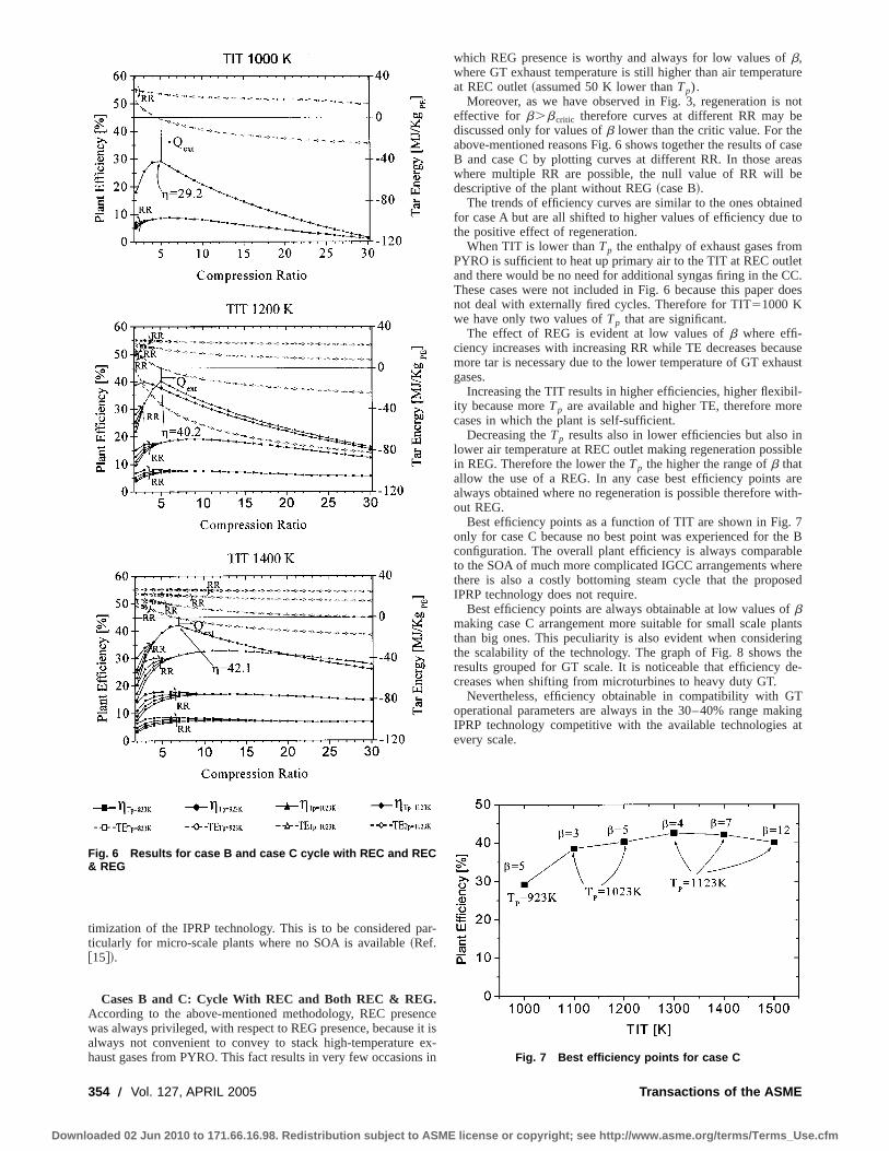
timization of the IPRP technology. This is to be considered par-ticularly for micro-scale plants where no SOA is available~Ref.@15#!.

Cases B and C: Cycle With REC and Both REC & REG.According to the above-mentioned methodology, REC presencewas always privileged, with respect to REG presence, because it isalways not convenient to convey to stack high-temperature ex-haust gases from PYRO. This fact results in very few occasions in

which REG presence is worthy and always for low values ofb,where GT exhaust temperature is still higher than air temperatureat REC outlet~assumed 50 K lower thanTp).

Moreover, as we have observed in Fig. 3, regeneration is noteffective for b.bcritic therefore curves at different RR may bediscussed only for values ofb lower than the critic value. For theabove-mentioned reasons Fig. 6 shows together the results of caseB and case C by plotting curves at different RR. In those areaswhere multiple RR are possible, the null value of RR will bedescriptive of the plant without REG~case B!.

The trends of efficiency curves are similar to the ones obtainedfor case A but are all shifted to higher values of efficiency due tothe positive effect of regeneration.

When TIT is lower thanTp the enthalpy of exhaust gases fromPYRO is sufficient to heat up primary air to the TIT at REC outletand there would be no need for additional syngas firing in the CC.These cases were not included in Fig. 6 because this paper doesnot deal with externally fired cycles. Therefore for TIT51000 Kwe have only two values ofTp that are significant.

The effect of REG is evident at low values ofb where effi-ciency increases with increasing RR while TE decreases becausemore tar is necessary due to the lower temperature of GT exhaustgases.

Increasing the TIT results in higher efficiencies, higher flexibil-ity because moreTp are available and higher TE, therefore morecases in which the plant is self-sufficient.

Decreasing theTp results also in lower efficiencies but also inlower air temperature at REC outlet making regeneration possiblein REG. Therefore the lower theTp the higher the range ofb thatallow the use of a REG. In any case best efficiency points arealways obtained where no regeneration is possible therefore with-out REG.

Best efficiency points as a function of TIT are shown in Fig. 7only for case C because no best point was experienced for the Bconfiguration. The overall plant efficiency is always comparableto the SOA of much more complicated IGCC arrangements wherethere is also a costly bottoming steam cycle that the proposedIPRP technology does not require.

Best efficiency points are always obtainable at low values ofbmaking case C arrangement more suitable for small scale plantsthan big ones. This peculiarity is also evident when consideringthe scalability of the technology. The graph of Fig. 8 shows theresults grouped for GT scale. It is noticeable that efficiency de-creases when shifting from microturbines to heavy duty GT.

Nevertheless, efficiency obtainable in compatibility with GToperational parameters are always in the 30–40% range makingIPRP technology competitive with the available technologies atevery scale.

Fig. 6 Results for case B and case C cycle with REC and REC& REG

Fig. 7 Best efficiency points for case C



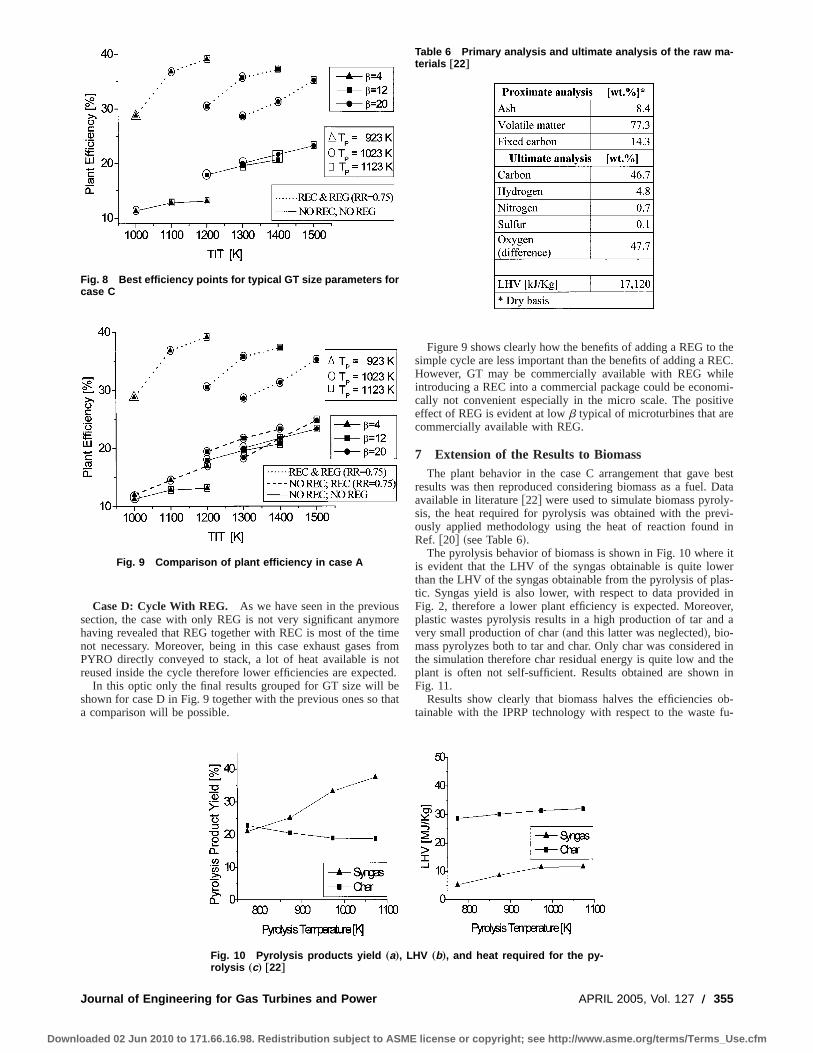
Case D: Cycle With REG. As we have seen in the previoussection, the case with only REG is not very significant anymorehaving revealed that REG together with REC is most of the timenot necessary. Moreover, being in this case exhaust gases fromPYRO directly conveyed to stack, a lot of heat available is notreused inside the cycle therefore lower efficiencies are expected.

In this optic only the final results grouped for GT size will beshown for case D in Fig. 9 together with the previous ones so thata comparison will be possible.

Figure 9 shows clearly how the benefits of adding a REG to thesimple cycle are less important than the benefits of adding a REC.However, GT may be commercially available with REG whileintroducing a REC into a commercial package could be economi-cally not convenient especially in the micro scale. The positiveeffect of REG is evident at lowb typical of microturbines that arecommercially available with REG.

7 Extension of the Results to BiomassThe plant behavior in the case C arrangement that gave best

results was then reproduced considering biomass as a fuel. Dataavailable in literature@22# were used to simulate biomass pyroly-sis, the heat required for pyrolysis was obtained with the previ-ously applied methodology using the heat of reaction found inRef. @20# ~see Table 6!.

The pyrolysis behavior of biomass is shown in Fig. 10 where itis evident that the LHV of the syngas obtainable is quite lowerthan the LHV of the syngas obtainable from the pyrolysis of plas-tic. Syngas yield is also lower, with respect to data provided inFig. 2, therefore a lower plant efficiency is expected. Moreover,plastic wastes pyrolysis results in a high production of tar and avery small production of char~and this latter was neglected!, bio-mass pyrolyzes both to tar and char. Only char was considered inthe simulation therefore char residual energy is quite low and theplant is often not self-sufficient. Results obtained are shown inFig. 11.

Results show clearly that biomass halves the efficiencies ob-tainable with the IPRP technology with respect to the waste fu-

Fig. 8 Best efficiency points for typical GT size parameters forcase C

Fig. 9 Comparison of plant efficiency in case A

Fig. 10 Pyrolysis products yield „a…, LHV „b…, and heat required for the py-rolysis „c… †22‡

Table 6 Primary analysis and ultimate analysis of the raw ma-terials †22‡



elled scenario. Best efficiency point show poor efficiencies for themicroscale~around 7%! and encouraging values for the interme-diate scale~around 16%!. It has to be noted that this result is alsoaffected by the use of char in post-combustion and not both charand tar therefore reducing prematurely the growing trend of effi-ciency curves in Fig. 11. This was assumed for technical reasonsconcerning the difficulty of burning tar in a char burner.

8 ConclusionsThis paper analyzes an innovative solution for waste and bio-

mass to energy conversion. The plant combines a rotary kiln py-rolyzer and a gas turbine fuelled by the pyrolysis gas produced

from the thermal degradation of residual fuels. The exhaust gasesfrom the gas turbine provide the heat required to maintain pyroly-sis while additional energy may be supplied by post-combustionof tars and chars produced by pyrolysis. Four plant configurationwere analyzed with different heat recovery solutions and for eachof them performance was evaluated by varying main thermody-namic parameters.

When fueled with a plastic-behaving residue, results obtainedfor the simple cycle with no regeneration show best efficienciesthat range from 11% for microscale plants to 23% for big scaleplants. The possibility of regenerating the Joule cycle with theexhaust gases exiting the pyrolyzer strongly enhances plant per-formance especially on the medium to small scale with results thatrange between 30 and 40%. Using a recuperated GT improvesefficiency only at low values of pressure ratio therefore it may beutilised only on the microscale.

When fueled with a wood-behaving residue the results obtainedshow similar trends but the efficiencies are halved due to thelower energetic content of the pyrolysis gas and the use of onlychar in post-combustion.

IPRP technology is a scalable concept because best efficiencypoints are obtainable for combinations of operational parametersthat are consistent with microturbines, aeroderivative, and heavyduty GT’s.

IPRP technology can perform as available technologies but at alower capital cost because no bottoming steam cycle is required.Moreover, IPRP technology provides a solution for the microscale where there are no available technologies.

Critical points of the proposed technology may be found invariable yields and energy content of pyrolysis products that mayjeopardize performance and produce combustion irregularities inboth the GT and TAR CC, and in syngas cleaning, that shallguarantee optimal performance of the syngas compressor and ofthe GT.

A laboratory scale rotary kiln was built at the University ofPerugia@23# providing experimental data on pyrolysis to back upnumerical simulation and the design of a microscale~70 kWe!IPRP pilot plant@24# that is being built at the Terni facility of theUniversity of Perugia with regional co-funding.

Nomenclature

B&W 5 biomass and wasteCp 5 specific heat at constant pressureCC 5 combustion chamber

COMP 5 compressorCYCLO 5 cyclone

GT 5 gas turbineICE 5 internal combustion engine

IGCC 5 integrated gasification combined cycleLHV 5 low heating value

m 5 mass flowP 5 pressure~Pa!

PYRO 5 pyrolyzerQ 5 heat (MJ/KgRF)

RDF 5 refuse derived fuelREC 5 recuperatorREG 5 regenerator

RF 5 residual fuelRR 5 regeneration ratio

SCR 5 scrubberSOA 5 state of the artSYN 5 syngas

T 5 temperature~K!TE 5 tar energy~from residual tar~char! combustion!

TIT 5 turbine inlet temperatureW 5 specific work (J/KgRF)b 5 compressor pressure ratiof 5 specific additional fuel consumption (kgNG /kgRF)

Fig. 11 Results obtained for case C biomass fueled



Subscripts

Air 5 airav 5 averageEg 5 exhaust gasesExt 5 external

In 5 inletNG 5 natural gasOut 5 outlet

P 5 pyrolysisRDF 5 refuse derived fuelREG 5 regenerator

RF 5 residual fuelSyn 5 syngas

T 5 turbine

References@1# UN Convention on Climate Change, 1997, Report of the conference of the

parties on its third session, held at Kyoto from 1 to 11 December, FCCC/CP/1997/7/Add. 1.

@2# van den Broek, R., Faaij, A., and van Wijk, A., 1996, ‘‘Biomass Combustionfor Power Generation,’’ Biomass Bioenergy,11, pp. 271–281.

@3# Stahl, K., and Neergaard, M., 1998, ‘‘IGCC Power Plant for Biomass Utilisa-tion, Varnamo, Sweden,’’ Biomass Bioenergy,15, pp. 205–211.

@4# Elmegaard, B., Henriksen, U., and Qvale, B., 2002, ‘‘Thermodynamic Analy-sis of Supplementary-Fired Gas Turbine Cycles,’’Proceedings of the Confer-ence ‘‘ECOS 2002’’.

@5# Elmegaard, B., Qvale, B., Carapelli, G., and De Faveri, P., 2001, ‘‘Open-CycleIndirectly Fired Gas Turbine for Wet Biomass Fuels,’’Proceedings of theConference ‘‘ECOS 2001,’’ July 4–6, Istanbul, Turkey.

@6# Solantausta, Y., Bridgwater, A. V., and Beckman, D., 1995, ‘‘Feasibility ofPower Production With Pyrolysis and Gasification Systems,’’ Biomass Bioen-ergy,9, pp. 257–269.

@7# Bridgwater, A. V., Elliot, D. C., Fagernas, L., Gifford, J. S., Mackie, K. L., andToft, A. J., 1995, ‘‘The Nature and Control of Solid, Liquid and GaseousEmissions From the Thermochemical Processing of Biomass,’’ BiomassBioenergy,9, pp. 325–341.

@8# Demirbas, A., 2001, ‘‘Carbonisation Ranking of Selected Biomass for Char-coal, Liquid and Gaseous Products,’’ Energy Convers. Manage.,42, pp. 1229–1238.

@9# Demirbas, A., 1997, ‘‘Calculation of Higher Heating Values of Biomass Fu-els,’’ Fuel, 76, pp. 431–434.

@10# Demirbas, A., 2000, ‘‘Mechanism of Liquefaction and Pyrolysis Reactions ofBiomass,’’ Energy Convers. Manage.,41, pp. 633–646.

@11# Di Blasi, C., and Branca, C., 2000, ‘‘Evaluation of the Performance of a NovelStraw Pyrolysis Reactor,’’ 1st World Conference on Biomass for Energy andIndustry, Sevilla, Spain, 5–9 June, pp. 1767–1770.

@12# Di Blasi, C., Signorelli, G., Di Russo, C., and Rea, G., 1999, ‘‘Product Distri-bution From Pyrolysis of Wood and Agricultural Residues,’’ Ind. Eng. Chem.Res.,38, pp. 2216–2224.

@13# Di Blasi, C., Signorelli, G., and Portoricco, G., 1999, ‘‘Countercurrent Fixed-Bed Gasification of Biomass at Laboratori Scale,’’ Ind. Eng. Chem. Res.,38,pp. 2571–2581.

@14# Roy, C., and Morin, D., 1998, ‘‘Efficient Electricity Production From BiomassThrough IPCC Power Plants,’’ 4th International Conference on GreenhouseGas Control Technologies~GHGT4!, Interlaken, Switzerland.

@15# Fantozzi, F., D’Alessandro, B., and Bidini, G., 2003, ‘‘IPRP—Integrated Py-rolysis Regenerated Plant—Gas Turbine and Externally Heated Rotary-KilnPyrolysis as a Biomass and Waste Energy Conversion System. Influence ofThermodynamic Parameters,’’ Proc. Inst. Mech. Eng., Part A: J. Power Energy217, pp. 519–527.

@16# Fantozzi, F., Di Maria, F., and Desideri, U., 2001, ‘‘Micro-Turbine Fuelled byPyrolysis Gas,’’Thermodynamic Analysis, Proceedings of the POWERGENEurope Congress and Exhibition, Helsinki.

@17# Fantozzi, F., Di Maria, F., and Desideri, U., 2002, ‘‘Integrated Micro-Turbineand Rotary Kiln Pyrolysis System as a Waste to Energy Solution for a SmallTown in Central Italy—Cost Positioning and Global Warming Assessment,’’ASME Paper GT-2002-30652.

@18# Li, A. M., Li, X. D., Ren, Y., Chi, Y., Yan, J. H., and Cen, K. F., 1999,‘‘Pyrolysis of Solid Waste in a Rotary Kiln: Influence of Final Pyrolysis Tem-perature on the Pyrolysis Products,’’ J. Anal. Appl. Pyrolysis,50, pp. 149–162.

@19# Yang, J., and Roy, C., 1996, ‘‘A New Method for DTA Measurement of En-thalpy Change During the Pyrolysis of Rubbers,’’ Thermochim. Acta,288, pp.155–168.

@20# Arcangioli, S., Gamberi, F., Milli, A., and Scapecchi, N., ‘‘Analysis of anIndirectly Biomass-Fired Gasturbine Engine Integrated With Pyrolysis forSupplementary Firing,’’ Biomass Gasification Group, Department of Mechani-cal Engineering, Technical University of Denmark~DTU! Internal Report.

@21# Neilson, C. E., 1998, ‘‘LM2500 Gas Turbine Modifications for Biomass FuelOperation,’’ Biomass Bioenergy,15, pp. 269–273.

@22# Encinar, J. M., Gonzalez, J. F., and Gonzalez, J., 2000, ‘‘Fixed-Bed Pyrolysisof Cynara Cardunculus L. Product Yields and Compositions,’’ Fuel Process.Technol.,68, pp. 209–222.

@23# Frantozzi, F., and Desideri, U., 2004, ‘‘Micro Scale Rotary Kiln Slow-Pyrolysis for Syngas and Char Production from Biomass and Waste: Reactorand Test Bench Realization,’’ ASME Paper GT-2004-54186.

@24# Bidini, G., Moriconi, A., Rossi, D., and Fantozzi, F., 2004, ‘‘IPRP—IntegratedPyrolysis Regenerated Plant Rotary Kiln Pyrolyzer and Microturbine for Dis-tributed Energy Conversion from Biomass—A 70 Kw Demonstration Unit inCentral Italy,’’ Proceedings of the Second World Conference and TechnologyExhibition on Biomass for Energy Industry and Clilmate Protection, May,Rome.



Shoko Itoe-mail: [email protected]

Hiroshi Saeki

Asako Inomata

Fumio Ootomo

Katsuya Yamashita

Yoshitaka Fukuyama1

Toshiba Corporation,Yokohama, Japan

Elichi Koda

Toru Takehashi

Mikio Satoe-mail: [email protected]

Central Research Institute of Electric PowerIndustry,

Yokosuka, Japan

Miki Koyama

Toru Ninomiyae-mail: [email protected]

New Energy and Industrial TechnologyDevelopment Organization,

Tokyo, Japan

Conceptual Design and CoolingBlade Development of 1700°CClass High-Temperature GasTurbineIn this paper we describe the conceptual design and cooling blade development of a1700°C-class high-temperature gas turbine in the ACRO-GT-2000 (Advanced CarbonDioxide Recovery System of Closed-Cycle Gas Turbine Aiming 2000 K) project. In theACRO-GT closed cycle power plant system, the thermal efficiency aimed at is more than60% of the higher heating value of fuel (HHV). Because of the high thermal efficiencyrequirement, the 1700°C-class high-temperature gas turbine must be designed with theminimum amount of cooling and seal steam consumption. The hybrid cooling scheme,which is a combination of closed loop internal cooling and film ejection cooling, waschosen from among several cooling schemes. The elemental experiments and numericalstudies, such as those on blade surface heat transfer, internal cooling channel heat trans-fer, and pressure loss and rotor coolant passage distribution flow phenomena, were con-ducted and the results were applied to the conceptual design advancement. As a result, thecooling steam consumption in the first stage nozzle and blade was reduced by about 40%compared with the previous design that was performed in the WE-NET (World EnergyNetwork) Phase-I.@DOI: 10.1115/1.1806456#

IntroductionIn regard to the greenhouse effect, there is a global and strong

demand to reduce CO2 emissions by the improvement of the ther-mal efficiency of power plants. The project entitled ACRO-GT-2000 was sponsored by the New Energy and Industrial Technol-ogy Development Organization of Japan~NEDO! and conductedfrom fiscal year 1999 to 2001. The aim of the project, which wasthe successor project to WE-NET Phase-I, was the development ofa 500 MW class thermal power plant with more than 60% HHVefficiency by using methane (CH4) fuel instead of hydrogen (H2)in the WE-NET project and free from CO2 emission due to recov-ery of the CO2 from exhaust gas. The purpose of the new projectis to promote the near-term realization of a highly efficient powerplant by utilizing more general and practical fuel, CH4 . And afundamental system study of a high-efficiency closed cycle powergeneration system has been performed and reported by Koda et al.@1#.

Several system studies have been performed for the CO2 recov-

ery power generation systems by other researchers. Jackson et al.@2# studied the closed topping cycle system for a CO2 and H2Ogas mixture with the sequestration of CO2 . Jeriche et al.@3# re-ported the conceptual design of a prototype 100 MW class Grazcycle power plant. In both cases, 1500°C~2370°F!-class gas tur-bine was assumed.

The present system features the introduction of the CH4-O2

combustion system and the 1700°C~3090°F!-class high-temperature gas turbine. It is well known that the increase inturbine inlet temperature has a strong impact on the thermal effi-ciency enhancement. However, the gas turbine working tempera-ture rise results in the increase of the coolant flow rate, under theturbine blade, with the same cooling structure, material, and ther-mal barrier coating~TBC!. And the increase of the coolant con-sumption deteriorates the thermal efficiency of the plant. So, forthe realization of high-temperature gas turbine, the developmentof a more efficient cooling structure, a more durable base-metaland a more effective insulation coating are essential.

The cooling structure selected for the first stage nozzle andblade was a hybrid cooling scheme that was developed and veri-fied by a high-temperature cascade experiment in the formerproject, WE-NET@4,5# To minimize the coolant flow rates, vari-ous elemental experiments and numerical studies have been car-ried out.

1Currently at Japan Aerospace Exploration Agency, Tokyo, Japan. E-mail:[email protected]

Contributed by the International Gas Turbine Institute~IGTI! of THE AMERICANSOCIETY OF MECHANICAL ENGINEERSfor publication in the ASME JOURNAL OFENGINEERING FOR GAS TURBINES AND POWER. Paper presented at the Interna-tional Gas Turbine and Aeroengine Congress and Exhibition, Atlanta, GA, June16–19; 2003, Paper No. 2003-GT-38352. Manuscript received by IGTI, October2002, final revision, March 2003. Associate Editor: H. R. Simmons.



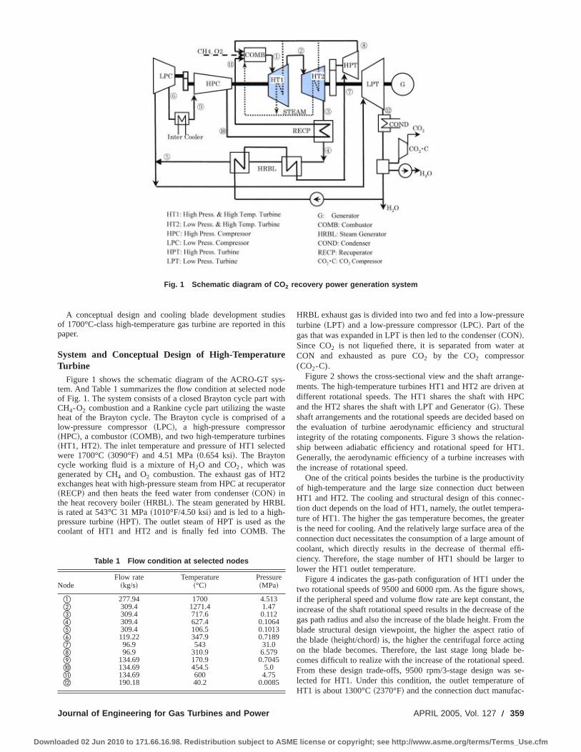
A conceptual design and cooling blade development studiesof 1700°C-class high-temperature gas turbine are reported in thispaper.

System and Conceptual Design of High-TemperatureTurbine

Figure 1 shows the schematic diagram of the ACRO-GT sys-tem. And Table 1 summarizes the flow condition at selected nodeof Fig. 1. The system consists of a closed Brayton cycle part withCH4-O2 combustion and a Rankine cycle part utilizing the wasteheat of the Brayton cycle. The Brayton cycle is comprised of alow-pressure compressor~LPC!, a high-pressure compressor~HPC!, a combustor~COMB!, and two high-temperature turbines~HT1, HT2!. The inlet temperature and pressure of HT1 selectedwere 1700°C~3090°F! and 4.51 MPa~0.654 ksi!. The Braytoncycle working fluid is a mixture of H2O and CO2 , which wasgenerated by CH4 and O2 combustion. The exhaust gas of HT2exchanges heat with high-pressure steam from HPC at recuperator~RECP! and then heats the feed water from condenser~CON! inthe heat recovery boiler~HRBL!. The steam generated by HRBLis rated at 543°C 31 MPa~1010°F/4.50 ksi! and is led to a high-pressure turbine~HPT!. The outlet steam of HPT is used as thecoolant of HT1 and HT2 and is finally fed into COMB. The

HRBL exhaust gas is divided into two and fed into a low-pressureturbine ~LPT! and a low-pressure compressor~LPC!. Part of thegas that was expanded in LPT is then led to the condenser~CON!.Since CO2 is not liquefied there, it is separated from water atCON and exhausted as pure CO2 by the CO2 compressor(CO2-C).

Figure 2 shows the cross-sectional view and the shaft arrange-ments. The high-temperature turbines HT1 and HT2 are driven atdifferent rotational speeds. The HT1 shares the shaft with HPCand the HT2 shares the shaft with LPT and Generator~G!. Theseshaft arrangements and the rotational speeds are decided based onthe evaluation of turbine aerodynamic efficiency and structuralintegrity of the rotating components. Figure 3 shows the relation-ship between adiabatic efficiency and rotational speed for HT1.Generally, the aerodynamic efficiency of a turbine increases withthe increase of rotational speed.

One of the critical points besides the turbine is the productivityof high-temperature and the large size connection duct betweenHT1 and HT2. The cooling and structural design of this connec-tion duct depends on the load of HT1, namely, the outlet tempera-ture of HT1. The higher the gas temperature becomes, the greateris the need for cooling. And the relatively large surface area of theconnection duct necessitates the consumption of a large amount ofcoolant, which directly results in the decrease of thermal effi-ciency. Therefore, the stage number of HT1 should be larger tolower the HT1 outlet temperature.

Figure 4 indicates the gas-path configuration of HT1 under thetwo rotational speeds of 9500 and 6000 rpm. As the figure shows,if the peripheral speed and volume flow rate are kept constant, theincrease of the shaft rotational speed results in the decrease of thegas path radius and also the increase of the blade height. From theblade structural design viewpoint, the higher the aspect ratio ofthe blade~height/chord! is, the higher the centrifugal force actingon the blade becomes. Therefore, the last stage long blade be-comes difficult to realize with the increase of the rotational speed.From these design trade-offs, 9500 rpm/3-stage design was se-lected for HT1. Under this condition, the outlet temperature ofHT1 is about 1300°C~2370°F! and the connection duct manufac-

Fig. 1 Schematic diagram of CO 2 recovery power generation system

Table 1 Flow condition at selected nodes

NodeFlow rate

~kg/s!Temperature

~°C!Pressure~MPa!

a 277.94 1700 4.513b 309.4 1271.4 1.47c 309.4 717.6 0.112d 309.4 627.4 0.1064e 309.4 106.5 0.1013f 119.22 347.9 0.7189g 96.9 543 31.0h 96.9 310.9 6.579i 134.69 170.9 0.7045j 134.69 454.5 5.0k 134.69 600 4.75l 190.18 40.2 0.0085



turing becomes feasible. For the 1300°C-class HT2, 3000 rpm/4-stage turbine design was selected. Table 2 summarizes the speci-fication of HT1 and HT2.

High-Temperature Turbine Cooling SystemFigure 5 indicates the schematic drawing of the HT1 cooling

system. The turbine rotor consists of three turbine disks, two spac-ers, rear shaft and intermediate shaft~which connects with HPC!,all of which are bolted together. The steam, individually suppliedfrom the casing side, cools the nozzles. On the other hand, rotorcooling steam is supplied from the bore of the rear shaft. The rearshaft and one to two stage spacer disk have many radial channelsto feed the coolant to the ring-shaped supply cavity just below theroot of the blades. The steam, which cools the blades internally, isaccumulated in the recovery cavity and then led to the combustor.This cooling steam flow also cools the rotor and spacer disks tosufficiently low temperature. Finally, a relatively small amount ofsteam is consumed as a hot gas seal at the disk to disk clearance.

In this type of internal cooling, the turbine hot parts such as thenozzle and blade act as a steam super-heater. And the thermalenergy transmitted from the hot main flow gas to coolant is recov-ered in the combustor.

Elemental Experiments

Rotor Center Bore and Radial Channels Flow. The steamflow in the rotor is complex, because of the rotational effects. And

the pressure loss characteristics may be different from that of thestationary case. To design the inside-rotor coolant distribution,pressure loss characteristics need to be clarified. Therefore, theexperimental measurements of the pressure loss of the rotor boreand radial distribution channel have been carried out.

Basically, the Coriolis and inertia force may dominate the flowin the rotating system under the gas turbine condition. So that inthe model experiments, the ratio of Reynolds numbers Rer overRv , namelyV, has been selected as the main experimental pa-rameter and made nearly equal to the HT1 condition. Rer , Rv ,and V in the experimental and HT1 conditions are listed inTable 3.

Rv5vd2/~2n! (1)

Rer5Vd/n (2)

V5Rv /Rer (3)

z5DP/~0.5r V2! (4)

Figure 6 shows the drawing of the test section. The axial inflowpassage~center bore! is 80 mm in diameter. The radial distributionchannels are 18.8 mm318.8 mm square and the number was 12. Aphotograph of the apparatus is shown in Fig. 7. Experiments werecarried out up to the rotational speed of 4000 rpm under the am-bient air condition.

Fig. 2 Structure of 1700°C class gas turbine

Fig. 3 Variation of adiabatic efficiency with rotational speed„HT1… Fig. 4 Gas path configuration „HT1…



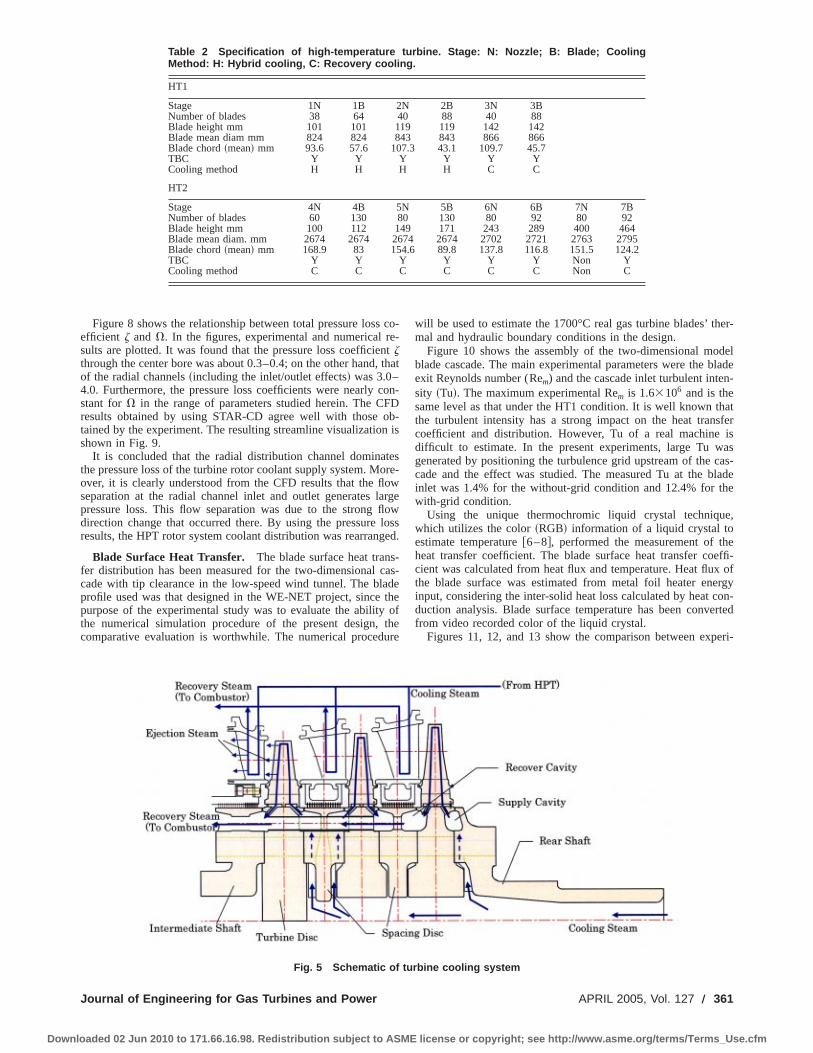
Figure 8 shows the relationship between total pressure loss co-efficient z and V. In the figures, experimental and numerical re-sults are plotted. It was found that the pressure loss coefficientzthrough the center bore was about 0.3–0.4; on the other hand, thatof the radial channels~including the inlet/outlet effects! was 3.0–4.0. Furthermore, the pressure loss coefficients were nearly con-stant forV in the range of parameters studied herein. The CFDresults obtained by using STAR-CD agree well with those ob-tained by the experiment. The resulting streamline visualization isshown in Fig. 9.

It is concluded that the radial distribution channel dominatesthe pressure loss of the turbine rotor coolant supply system. More-over, it is clearly understood from the CFD results that the flowseparation at the radial channel inlet and outlet generates largepressure loss. This flow separation was due to the strong flowdirection change that occurred there. By using the pressure lossresults, the HPT rotor system coolant distribution was rearranged.

Blade Surface Heat Transfer. The blade surface heat trans-fer distribution has been measured for the two-dimensional cas-cade with tip clearance in the low-speed wind tunnel. The bladeprofile used was that designed in the WE-NET project, since thepurpose of the experimental study was to evaluate the ability ofthe numerical simulation procedure of the present design, thecomparative evaluation is worthwhile. The numerical procedure

will be used to estimate the 1700°C real gas turbine blades’ ther-mal and hydraulic boundary conditions in the design.

Figure 10 shows the assembly of the two-dimensional modelblade cascade. The main experimental parameters were the bladeexit Reynolds number (Rem) and the cascade inlet turbulent inten-sity ~Tu!. The maximum experimental Rem is 1.63106 and is thesame level as that under the HT1 condition. It is well known thatthe turbulent intensity has a strong impact on the heat transfercoefficient and distribution. However, Tu of a real machine isdifficult to estimate. In the present experiments, large Tu wasgenerated by positioning the turbulence grid upstream of the cas-cade and the effect was studied. The measured Tu at the bladeinlet was 1.4% for the without-grid condition and 12.4% for thewith-grid condition.

Using the unique thermochromic liquid crystal technique,which utilizes the color~RGB! information of a liquid crystal toestimate temperature@6–8#, performed the measurement of theheat transfer coefficient. The blade surface heat transfer coeffi-cient was calculated from heat flux and temperature. Heat flux ofthe blade surface was estimated from metal foil heater energyinput, considering the inter-solid heat loss calculated by heat con-duction analysis. Blade surface temperature has been convertedfrom video recorded color of the liquid crystal.

Figures 11, 12, and 13 show the comparison between experi-

Fig. 5 Schematic of turbine cooling system

Table 2 Specification of high-temperature turbine. Stage: N: Nozzle; B: Blade; CoolingMethod: H: Hybrid cooling, C: Recovery cooling.

HT1

Stage 1N 1B 2N 2B 3N 3BNumber of blades 38 64 40 88 40 88Blade height mm 101 101 119 119 142 142Blade mean diam mm 824 824 843 843 866 866Blade chord~mean! mm 93.6 57.6 107.3 43.1 109.7 45.7TBC Y Y Y Y Y YCooling method H H H H C C

HT2

Stage 4N 4B 5N 5B 6N 6B 7N 7BNumber of blades 60 130 80 130 80 92 80 92Blade height mm 100 112 149 171 243 289 400 464Blade mean diam. mm 2674 2674 2674 2674 2702 2721 2763 2795Blade chord~mean! mm 168.9 83 154.6 89.8 137.8 116.8 151.5 124.2TBC Y Y Y Y Y Y Non YCooling method C C C C C C Non C



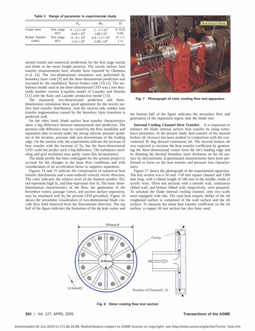
mental results and numerical predictions for the first stage nozzleand blade at the mean height position. The nozzle surface heattransfer measurements have already been reported by Okamuraet al. @4#. The two-dimensional simulation was performed byboundary layer code@9# and the three-dimensional prediction wasexecuted by the multiblock Navier-Stokes code@10,11#. The tur-bulence model used in the three-dimensional CFD was a low Rey-nolds number version k-epsilon model of Launder and Sharma@12# with the Kato and Launder production model@13#.

The measured, two-dimensional prediction and three-dimensional simulation show good agreement for the nozzle sur-face heat transfer distribution. And the suction side sudden heattransfer augmentation caused by the boundary layer transition ispredicted well.

On the other hand, blade surface heat transfer characteristicsshow a big difference between measurement and prediction. Thepressure side difference may be caused by the flow instability andseparation that occurred under the strong adverse pressure gradi-ent at the location, pressure side just downstream of the leadingedge. On the suction side, the experiments indicate the increase ofheat transfer with the increase of Tu, but the three-dimensionalCFD could not predict such a big difference. The turbulence mod-eling and grid resolution may partly cause this inconsistency.

The blade profile has been redesigned for the present project toaccount for the changes in the main flow conditions and withconsideration of an acceleration factor to suppress separation.

Figures 14 and 15 indicate the visualization of numerical heattransfer distributions and a near-endwall velocity vector direction.The color indicates the relative level of the Stanton number~St!,red represents high St, and blue represents low St. The basic three-dimensional characteristics of the flow, the generation of thehorseshoe vortex, passage vortex, and suction surface separation,may be simulated well by the present CFD procedure. Figure 16shows the streamline visualization of two-dimensional blade cas-cade flow field observed from the downstream direction. The tophalf of the figure indicates the formation of the tip leak vortex and

the bottom half of the figure indicates the secondary flow andgeneration of the separation region near the blade root.

Internal Cooling Channel Heat Transfer. It is important toenhance the blade internal surface heat transfer by using turbu-lence promoters. In the present study, heat transfer of the skewedbroken rib~4-rows! has been studied in comparison with the con-ventional 45 deg skewed continuous rib. The skewed broken ribwas expected to increase the heat transfer coefficient by generat-ing the three-dimensional vortex from the rib’s leading edge andby thinning the thermal boundary layer thickness on the rib sur-face by discontinuity. Experimental measurements have been per-formed to focus on the heat transfer and pressure loss character-istics.

Figure 17 shows the photograph of the experimental apparatus.The test section was a 50 mm350 mm square channel and 1300mm long, with a ribbed length of 540 mm in the middle, made ofacrylic resin. Three test sections with a smooth wall, continuousribbed wall, and broken ribbed wall, respectively, were prepared.To simulate the blade internal cooling channel, only two wallswere equipped with ribs. The total heat transfer ability of the ribroughened surface is comprised of the wall surface and the ribsurface. To measure the mean heat transfer coefficient on the ribsurface, a copper rib test section has also been used.

Fig. 6 Rotor cooling flow test section

Fig. 7 Photograph of rotor cooling flow test apparatus

Table 3 Range of parameter in experimental study

Rv Rer V

Center bore Test range 0 – 1.23105 2 – 53105 0–0.43HT1 9.833106 1.483107 0.66

Radial channel~inlet!

Test range 0 – 63104 0.4– 1.13105 0–1.3HT1 2.313106 2.083106 1.11



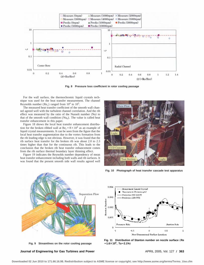
For the wall surface, the thermochromic liquid crystals tech-nique was used for the heat transfer measurement. The channelReynolds number (Rec) ranged from 104 to 105.

The measured heat transfer coefficient of the smooth wall chan-nel agreed well with the turbulent channel correlation. And the ribeffect was measured by the ratio of the Nusselt number~Nu! tothat of the smooth wall condition (Nu0). The value is called heattransfer enhancement in this paper.

Figure 18 shows the local heat transfer enhancement distribu-tion for the broken ribbed wall at Rec583104 as an example ofliquid crystal measurements. It can be seen from the figure that thelocal heat transfer augmentation due to the vortex formation fromthe rib leading edge is not obvious. However, it was found that therib surface heat transfer for the broken rib was about 2.0 to 2.3times higher than that for the continuous rib. This leads to theconclusion that the broken rib heat transfer enhancement comesfrom the rib surface thermal boundary layer thinning effect.

Figure 19 indicates the Reynolds number dependency of meanheat transfer enhancement including both walls and rib surfaces. Itwas found that the present smooth side wall results agreed well

Fig. 8 Pressure loss coefficient in rotor cooling passage

Fig. 9 Streamlines on the rotor cooling passage

Fig. 10 Photograph of heat transfer cascade test apparatus

Fig. 11 Distribution of Stanton number on nozzle surface „ReÄ1.6Ã106, TuÄ2.1%…



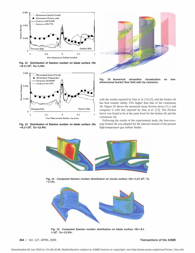
with the results reported by Han et al.@14,15#, and the broken ribhas heat transfer ability 25% higher than that of the continuousrib. Figure 20 shows the measured mean friction factor (Cf) andcompares it with that reported by Han et al.@15#. The frictionfactor was found to be at the same level for the broken rib and thecontinuous rib.

Following the results of the experimental study, the four-rows-type broken rib was adopted for the internal channel of the presenthigh-temperature gas turbine blades.

Fig. 12 Distribution of Stanton number on blade surface „ReÄ8.1Ã105, TuÄ1.4%…

Fig. 13 Distribution of Stanton number on blade surface „ReÄ8.1Ã105, TuÄ12.4%…

Fig. 14 Computed Stanton number distribution on nozzle surface „ReÄ1.6Ã106, TuÄ2.1%…

Fig. 15 Computed Stanton number distribution on blade surface „ReÄ8.1Ã105, TuÄ12.4%…

Fig. 16 Numerical streamline visualization on two-dimensional bucket flow field with tip clearance



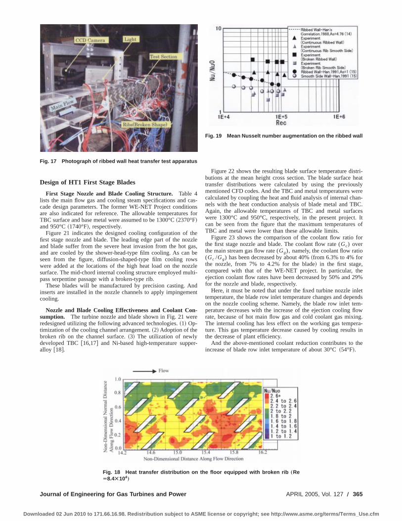
Design of HT1 First Stage Blades

First Stage Nozzle and Blade Cooling Structure. Table 4lists the main flow gas and cooling steam specifications and cas-cade design parameters. The former WE-NET Project conditionsare also indicated for reference. The allowable temperatures forTBC surface and base metal were assumed to be 1300°C~2370°F!and 950°C~1740°F!, respectively.

Figure 21 indicates the designed cooling configuration of thefirst stage nozzle and blade. The leading edge part of the nozzleand blade suffer from the severe heat invasion from the hot gas,and are cooled by the shower-head-type film cooling. As can beseen from the figure, diffusion-shaped-type film cooling rowswere added at the locations of the high heat load on the nozzlesurface. The mid-chord internal cooling structure employed multi-pass serpentine passage with a broken-type rib.

These blades will be manufactured by precision casting. Andinserts are installed in the nozzle channels to apply impingementcooling.

Nozzle and Blade Cooling Effectiveness and Coolant Con-sumption. The turbine nozzle and blade shown in Fig. 21 wereredesigned utilizing the following advanced technologies.~1! Op-timization of the cooling channel arrangement.~2! Adoption of thebroken rib on the channel surface.~3! The utilization of newlydeveloped TBC@16,17# and Ni-based high-temperature supper-alloy @18#.

Figure 22 shows the resulting blade surface temperature distri-butions at the mean height cross section. The blade surface heattransfer distributions were calculated by using the previouslymentioned CFD codes. And the TBC and metal temperatures werecalculated by coupling the heat and fluid analysis of internal chan-nels with the heat conduction analysis of blade metal and TBC.Again, the allowable temperatures of TBC and metal surfaceswere 1300°C and 950°C, respectively, in the present project. Itcan be seen from the figure that the maximum temperatures ofTBC and metal were lower than these allowable limits.

Figure 23 shows the comparison of the coolant flow ratio forthe first stage nozzle and blade. The coolant flow rate (Gc) overthe main stream gas flow rate (Gg), namely, the coolant flow ratio(Gc /Gg) has been decreased by about 40%~from 6.3% to 4% forthe nozzle, from 7% to 4.2% for the blade! in the first stage,compared with that of the WE-NET project. In particular, theejection coolant flow rates have been decreased by 50% and 29%for the nozzle and blade, respectively.

Here, it must be noted that under the fixed turbine nozzle inlettemperature, the blade row inlet temperature changes and dependson the nozzle cooling scheme. Namely, the blade row inlet tem-perature decreases with the increase of the ejection cooling flowrate, because of hot main flow gas and cold coolant gas mixing.The internal cooling has less effect on the working gas tempera-ture. This gas temperature decrease caused by cooling results inthe decrease of plant efficiency.

And the above-mentioned coolant reduction contributes to theincrease of blade row inlet temperature of about 30°C~54°F!.

Fig. 17 Photograph of ribbed wall heat transfer test apparatus

Fig. 18 Heat transfer distribution on the floor equipped with broken rib „ReÄ8.4Ã104

…

Fig. 19 Mean Nusselt number augmentation on the ribbed wall



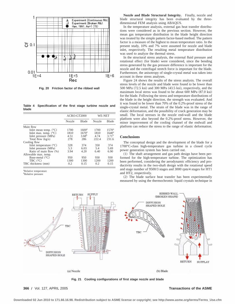
Nozzle and Blade Structural Integrity. Finally, nozzle andblade structural integrity has been evaluated by the three-dimensional FEM analysis using ABAQUS.

In the temperature analysis, external gas heat transfer distribu-tions were considered as in the previous section. However, themean gas temperature distribution in the blade height directionwas treated by the simple pattern factor-based method. The patternfactor is a measure of the highest to mean temperature ratio. In thepresent study, 10% and 7% were assumed for nozzle and bladeinlet, respectively. The resulting metal temperature distributionwas used to analyze the thermal stress.

In the structural stress analysis, the external fluid pressure androtational effect~for blade! were considered, since the bendingstress generated by the gas pressure difference is important for thenozzle and the centrifugal stretch force is important for the blade.Furthermore, the anisotropy of single-crystal metal was taken intoaccount in these stress analyses.

Figure 24 shows the results of the stress analysis. The overallstress levels of the nozzle and blade were found to be lower than500 MPa~72.5 ksi! and 300 MPa~43.5 ksi!, respectively, and themaximum local stress was found to be about 600 MPa~87.0 ksi!for the blade. Following the stress and temperature distributions ofthe blade in the height direction, the strength was evaluated. Andit was found to be lower than 70% of the 0.2%-proof stress of thesingle-crystal metal. The strain of the blade was in the range ofelastic deformation, and the possibility of crack generation may besmall. The local stresses in the nozzle end-wall and the bladeplatform were also beyond the 0.2%-proof stress. However, theminor improvement of the cooling channel of the endwall andplatform can reduce the stress to the range of elastic deformation.

ConclusionsThe conceptual design and the development of the blade for a

1700°C-class high-temperature gas turbine in a closed cyclepower generation system has been carried out.

~1! The shaft arrangement and gas path design have been per-formed for the high-temperature turbine. The optimization hasbeen performed, considering the aerodynamic efficiency and pro-ductivity results in the two-shaft design with the rotational speedand stage number of 9500/3 stages and 3000 rpm/4 stages for HT1and HT2, respectively.

~2! The blade surface heat transfer has been experimentallymeasured by using the thermochromic liquid crystals technique in

Fig. 20 Friction factor of the ribbed wall

Fig. 21 Cooling configurations of first stage nozzle and blade

Table 4 Specification of the first stage turbine nozzle andblade

ACRO-GT2000 WE-NET

Nozzle Blade Nozzle Blade

Main flowInlet mean temp.~°C! 1700 1600a 1700 1570a

Inlet max. temp.~°C! 1810 1670a 1810 1640a

Inlet pressure~MPa! 4.51 3.68b 4.74 3.71b

Total flow ~kg/s! 278 286 222.4 231.6Cooling flow

Inlet temperature~°C! 328 374 350 374Inlet pressure~MPa! 5.3 6.03 5.4 5.69Ratio of main flow~%! 3.94 4.20 6.40 6.90

Allowable max. temp.Base-metal~°C! 950 950 930 930TBC ~°C! 1300 1300 1200 1200

TBC thickness~mm! 0.2 0.15 0.2 0.15

aRelative temperaturebRelative pressure



Fig. 22 Blade mean height temperatures distributions

Fig. 23 A comparison of the coolant flow rate for the first stage nozzle and blade

Fig. 24 Nozzle and blade surface stress distributions



the low-pressure wind tunnel and the design of the three-dimensional numerical simulation code has been evaluated. Theresults suggest that the numerical prediction is partly valid for theheat transfer analysis.

~3! The broken rib-type turbulence promoter heat transfer andpressure loss have been measured. It was found that the overallheat transfer ability including the wall surface and the rib wasabout 25% higher than in the case of a continuous rib. This in-crease in heat transfer is due to the heat transfer increase of about2.0 to 2.3 times on the rib surface. So, the broken rib was adoptedfor the cooling design advancement.

~4! The pressure loss of the inter-rotor center bore and the dis-tribution radial passage has been evaluated by a model experi-ment. Based on the experimental results, rotor system flow distri-bution and coolant supply pressure have been rearranged.

~5! The redesigned hybrid cooling first stage nozzle and bladerealized a decrease of about 40% in coolant consumption com-pared with that of the WE-NET 1700°C stage. In particular, the50% ejection coolant reduction at the first stage nozzle can in-crease the blade row inlet gas temperature by about 30°C. Thiscontributes to the increase of plant thermal efficiency.

~6! The structural integrity of the first-stage nozzle and bladehas been evaluated by FEM thermal and structural stress analysis.And it was confirmed that the effective stress was well below the0.2% proof-stress of the base metal.

The conceptual design phase of the project has been finished.However, the confirmation and the operating experience accumu-lation for the complex closed-loop Brayton cycle/Rankin cyclesystem and the long-term durability tests for the newly introducedmaterials are necessary for the realization.

AcknowledgmentsThis work was supported by the New Energy and Industrial

Technology Development Organization~NEDO! as part of theACRO-GT-2000 program, and was directly entrusted by the Cen-tral Research Institute of Electric Power Industry~CRIEPI!. Theauthors would like to thank these organizations for their support.

Nomenclature

As 5 channel aspect ratioCf 5 friction factor

d 5 diameter~m!Gc 5 cooling mass flow rate~kg/s!Gg 5 main stream~hot! gas flow rate~kg/s!Nu 5 Nusselt number

Nu0 5 Nusselt number for smooth wallRec 5 Reynolds number for channelRem 5 Reynolds number for bladeRer 5 Reynolds number for rotor cooling passageRv 5 rotational Reynolds numberSt 5 Stanton numberTu 5 inlet turbulence intensityV 5 velocity ~m/s!

DP 5 pressure drop~Pa!

r 5 density~kg/m3!h t 5 turbine adiabatic efficiency

h td 5 turbine adiabatic efficiency at design pointz 5 total pressure loss coefficientn 5 kinetic viscosity~m2/s!v 5 rotational speed~1/s!V 5 rotational ratio (5Rv /Rer)

References@1# Koda, E., Takahashi, T., Uematsu, K., and Yamashita, K., 2002, ‘‘Study on the

Highly Efficient Closed-Cycle Gas Turbine System for CO2 Collection,’’ J.Gas Turbine Soc. Jpn.,30, pp. 63–67~in Japanese!.

@2# Jackson, J. B. A., Neto, A. C., Whellens, M., and Audus, 2000, ‘‘Gas TurbinePerformance Using Carbon Dioxide as Working Fluid in Closed Cycle Opera-tion,’’ ASME, 2000-GT-153.

@3# Jeriche, H., and Gottlich, E., 2002, ‘‘Conceptual Design for An IndustrialPrototype Graz Cycle Power Plant,’’ ASME, GT-2002-30118.

@4# Okamura, T., Koga, A., Ito, S., and Kawagishi, H., 2000, ‘‘Evaluation of1700°C Class Turbine Blades in Hydrogen Fueled Combustion Turbine Sys-tem,’’ ASME, 2000-GT-0615.

@5# Ito, S., Koga, A., Kawagishi, H., Matsuda, H., Suga, T., and Okamura, T.,2000, ‘‘Hydrogen Combustion Wind Tunnel Test of 1700°C Class TurbineCooling Blades,’’ J. Gas Turbine Soc. Jpn.,28, pp. 23–28~in Japanese!.

@6# Matsuda, H., Ikeda, K., Nakata, Y., Otomo, F., Suga, T., and Fukuyama, Y.,1999, ‘‘A New Thermochromic Liquid Crystal Temperature IdentificationTechnique Using Color Space Interpolations and Its Application to Film Cool-ing Effectiveness Measurements,’’Proceedings of PSFVIP-2, PF053.

@7# Saeki, H., Ito, S., Matsuda, H., and Okamura, T., 1999, ‘‘Heat Transfer Mea-surements on Turbine Nozzle Using Liquid Crystals,’’International Gas Tur-bine Congress ’99 Kobe, TS-47, pp. 607–613.

@8# Saeki, H., and Fukuyama, Y., 2002, ‘‘Heat Transfer Measurements on a GasTurbine Blade for ACRO-GT-2000,’’ ISROMAC-9, Paper HT-ABS-025.

@9# Biswas, D., and Fukuyama, Y., 1993, ‘‘Calculation of Transitional BoundaryLayer With an Improved Low Reynolds Number Version of the k-« TurbulenceModel,’’ ASME, 93-GT-73.

@10# Fukuyama, Y., Otomo, F., Sato, M., Kobayashi, Y., and Matsuzaki, H., 1995,‘‘Prediction of Vane Surface Film Cooling Effectiveness Using CompressibleNavier–Stokes Procedure and k-Epsilon Turbulence Model With Wall Func-tion,’’ ASME, 95-GT-25.

@11# Kubo, R., Otomo, F., Fukuyama, Y., and Nakata, Y., 1998, ‘‘Aerodynamic LossIncrease Due to Individual Film Cooling Injections From Gas Turbine NozzleSurface,’’ ASME, 98-GT-497.

@12# Launder, B. E., and Sharma, B. I., 1979, ‘‘Application of the Energy-Dissipation Model of Turbulence to the Calculation of Flow Near a SpinningDisc,’’ Lett. Heat Mass Transfer,1, pp. 131–138.

@13# Kato, M., and Launder, B. E., 1993, ‘‘The Modeling of Turbulent Flow AroundStationary and Vibrating Square Cylinders,’’ 9thSymposium on TurbulentShear Flows, Kyoto Japan, 10-4.

@14# Han, J. C., and Park, J. S., 1988, ‘‘Developing Heat Transfer in RectangularChannels With Rib Turbulators,’’ Int. J. Heat Mass Transfer,31, pp. 183–195.

@15# Han, J. C., Zhang, Y. M., and Lee, C. P., 1991, ‘‘Augmented Heat Transfer inSquare Channels With Parallel, Crossed, and V-Shaped Angled Ribs,’’ ASMEJ. Heat Transfer,113, pp. 590–596.

@16# Hisamatsu, T., 2002, ‘‘Development of Thermal Barrier Coating forCO2-Recovering Closed Gas Turbine,’’ J. Gas Turbine Soc. Jpn.,30, pp. 519–525 ~in Japanese!.

@17# Hisamatsu, T., Nitta, A., Nakayama, M., Torigoe, T., Mori, K., Okada, I., Hino,T., Kameda, T., Ito, Y., Arikawa, H., Kojima, Y., and Nishi, K., 2002, ‘‘Devel-opment and Evaluation of Thermal Barrier Coating for 1700°C-Class GasTurbine in the CO2-Turbine Project,’’ Report of the 123rd Committee on Heat-Resisting Materials and Alloys Japan Society for Promotion of Science, Vol.43, No. 3, pp. 325–340~in Japanese!.

@18# Koizumi, Y., Kobayashi, T., Yokokawa, T., Kimura, T., Osawa, M., andHarada, H., 1998, ‘‘Third Generation Single Crystal Superalloys With Excel-lent Processability and Phase Stability,’’Proceedings of Materials for Ad-vanced Power Engineering 1998, Part II, pp. 1089–1098.



Y. FukuizumiMitsubishi Heavy Industries,

3-1, Minatomirai 3-chome, Nishi-ku,Yokohama, Kanagawa 220-8401, Japan

J. Masada

V. Kallianpur

Mitsubishi Power Systems,2287 Premier Row,Orlando, FL 32809

Y. IwasakiMitsubishi Heavy Industries,

2-1-1 Shinhama Arai-cho,Takasago, Hyogo 676-8686, Japan

Application of ‘‘H Gas Turbine’’Design Technology to IncreaseThermal Efficiency and OutputCapability of the MitsubishiM701G2 Gas TurbineMitsubishi completed design development and verification load testing of a steam-cooledM501H gas turbine at a combined cycle power plant at Takasago, Japan in 2001. Severaladvanced technologies were specifically developed in addition to the steam-cooled com-ponents consisting of the combustor, turbine blades, vanes, and the rotor. Some of theother key technologies consisted of an advanced compressor with a pressure ratio of 25:1,active clearance control, and advanced seal technology. Prior to the M501H, Mitsubishiintroduced cooling-steam in ‘‘G series’’ gas turbines in 1997 to cool combustor liners.Recently, some of the advanced design technologies from the M501H gas turbine wereapplied to the G series gas turbine resulting in significant improvement in output andthermal efficiency. A noteworthy aspect of the technology transfer is that the upgraded Gseries M701G2 gas turbine has an almost equivalent output and thermal efficiency as Hclass gas turbines while continuing to rely on conventional air cooling of turbine bladesand vanes, and time-proven materials from industrial gas turbine experience. In thispaper we describe the key design features of the M701G2 gas turbine that make thispossible such as the advanced 21:1 compressor with 14 stages, an advanced premix DLNcombustor, etc., as well as shop load test results that were completed in 2002 at Mitsub-ishi’s in-house facility.@DOI: 10.1115/1.1850490#

1 IntroductionThe M701G2 gas turbine is built by enhancing the original

M701G with some of the advanced technologies that were devel-oped for Mitsubishi’s steam-cooled M501H gas turbine@1#. Theoriginal M701G gas turbines went into commercial operation in1999, and the lead unit has logged more than 25 000 operatinghours at close to 100% reliability. The M701G2 is presently Mit-subishi’s most advanced commercial offering for the 50 Hz powergeneration market. Table 1 compares the performance of theM701G and the M701G2 gas turbines. Note that the latter has asimple cycle efficiency and output of 39.5% and 334 MW, respec-tively. For a 131 combined cycle configuration those figures forthe M701G2 are 58.7% and 489 MW, respectively. The primarydesign approach of the M701G2 gas turbine was to introduce keyH technologies, without upsetting the proven reliability trackrecord of the original M701G gas turbine. Greater output andperformance were achieved by using an advanced compressorwith 15% greater mass flow, and a pressure ratio of 21:1. The onlysteam-cooled hardware in the M701G2 consist of the combustortransitions, and the turbine blade rings, whereas in the originalM701G gas turbine only the combustor transitions are steamcooled. On the other hand, the steam-cooled components in theM501H gas turbine consist of combustor transitions, blade rings,row 1 and row 2 turbine blades and vanes, and the rotor.

The full-scale load verification test of the steam-cooled M501Hgas turbine in a combined cycle power plant was completed suc-cessfully in 2001. New technologies were applied in the develop-

ment of the M501H for its 15 stage 25:1 pressure ratio compressorand steam cooled components. These include advanced 3D aero,mass transport and heat transfer analytical techniques and criticalmaterial compatiability evaluations for long-term reliability in asteam environment@2#.

The selective advanced technologies from the M501H develop-ment were applied to increase the output and performance of theoriginal M701G dramatically.

Table 2 compares the M701G2 with previous 50 Hz gas tur-bines from Mitsubishi. The development approach retained thesame evolution path such as retaining design feature commonalityand scaling practices across the 50 and 60 Hz models. A factoryload test of the M701G2 was conducted to further confirm thereliability of the gas turbine.

2 Design FeaturesFigure 1 shows a picture of the M701G2 gas turbine rotor. The

unit rotor is of bolted construction. There are 12 bolts in the com-pressor, and 12 in the turbine in conjunction with positive torquecarrying features such as radial pins and curvic couplings, respec-tively. The rotor is supported by two 23-in. diameter two-element


Table 1 Performance of M701G vs M701G2

Performance M701G M701G2

G/T Power~MW! 271 334G/T thermal efficiency~%—LHV!

38.7 39.5

Combined cycle~1 on 1!power ~MW!

405 489

Combined cycle~1 on 1!efficiency ~%—LHV!

57.0 58.7



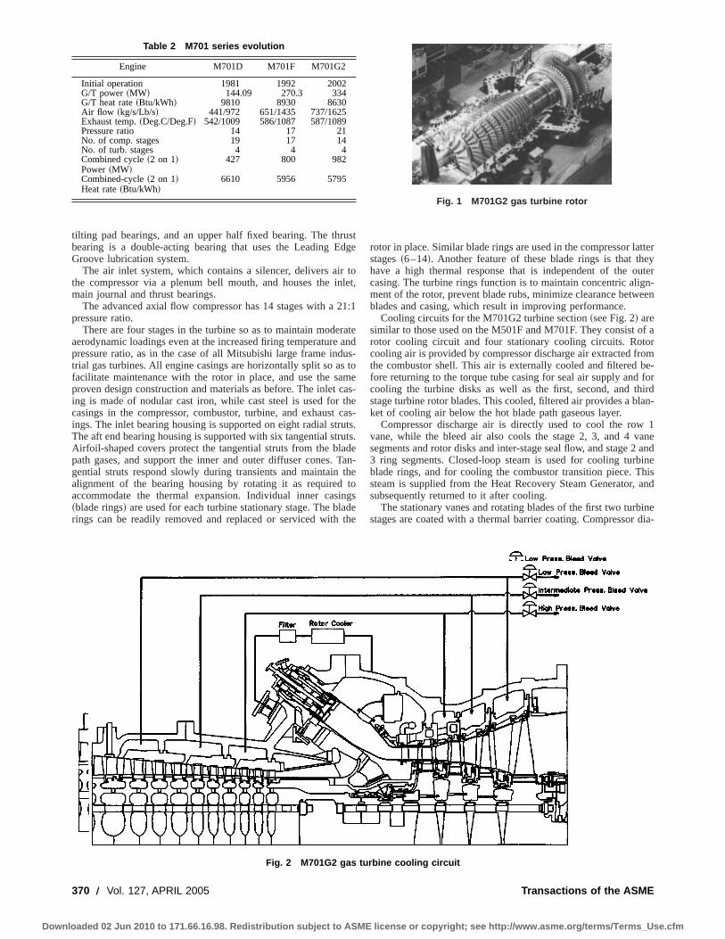
tilting pad bearings, and an upper half fixed bearing. The thrustbearing is a double-acting bearing that uses the Leading EdgeGroove lubrication system.

The air inlet system, which contains a silencer, delivers air tothe compressor via a plenum bell mouth, and houses the inlet,main journal and thrust bearings.

The advanced axial flow compressor has 14 stages with a 21:1pressure ratio.

There are four stages in the turbine so as to maintain moderateaerodynamic loadings even at the increased firing temperature andpressure ratio, as in the case of all Mitsubishi large frame indus-trial gas turbines. All engine casings are horizontally split so as tofacilitate maintenance with the rotor in place, and use the sameproven design construction and materials as before. The inlet cas-ing is made of nodular cast iron, while cast steel is used for thecasings in the compressor, combustor, turbine, and exhaust cas-ings. The inlet bearing housing is supported on eight radial struts.The aft end bearing housing is supported with six tangential struts.Airfoil-shaped covers protect the tangential struts from the bladepath gases, and support the inner and outer diffuser cones. Tan-gential struts respond slowly during transients and maintain thealignment of the bearing housing by rotating it as required toaccommodate the thermal expansion. Individual inner casings~blade rings! are used for each turbine stationary stage. The bladerings can be readily removed and replaced or serviced with the

rotor in place. Similar blade rings are used in the compressor latterstages~6–14!. Another feature of these blade rings is that theyhave a high thermal response that is independent of the outercasing. The turbine rings function is to maintain concentric align-ment of the rotor, prevent blade rubs, minimize clearance betweenblades and casing, which result in improving performance.

Cooling circuits for the M701G2 turbine section~see Fig. 2! aresimilar to those used on the M501F and M701F. They consist of arotor cooling circuit and four stationary cooling circuits. Rotorcooling air is provided by compressor discharge air extracted fromthe combustor shell. This air is externally cooled and filtered be-fore returning to the torque tube casing for seal air supply and forcooling the turbine disks as well as the first, second, and thirdstage turbine rotor blades. This cooled, filtered air provides a blan-ket of cooling air below the hot blade path gaseous layer.

Compressor discharge air is directly used to cool the row 1vane, while the bleed air also cools the stage 2, 3, and 4 vanesegments and rotor disks and inter-stage seal flow, and stage 2 and3 ring segments. Closed-loop steam is used for cooling turbineblade rings, and for cooling the combustor transition piece. Thissteam is supplied from the Heat Recovery Steam Generator, andsubsequently returned to it after cooling.

The stationary vanes and rotating blades of the first two turbinestages are coated with a thermal barrier coating. Compressor dia-

Fig. 1 M701G2 gas turbine rotor

Fig. 2 M701G2 gas turbine cooling circuit

Table 2 M701 series evolution

Engine M701D M701F M701G2

Initial operation 1981 1992 2002G/T power~MW! 144.09 270.3 334G/T heat rate~Btu/kWh! 9810 8930 8630Air flow ~kg/s/Lb/s! 441/972 651/1435 737/1625Exhaust temp.~Deg.C/Deg.F! 542/1009 586/1087 587/1089Pressure ratio 14 17 21No. of comp. stages 19 17 14No. of turb. stages 4 4 4Combined cycle~2 on 1!Power~MW!

427 800 982

Combined-cycle~2 on 1!Heat rate~Btu/kWh!

6610 5956 5795



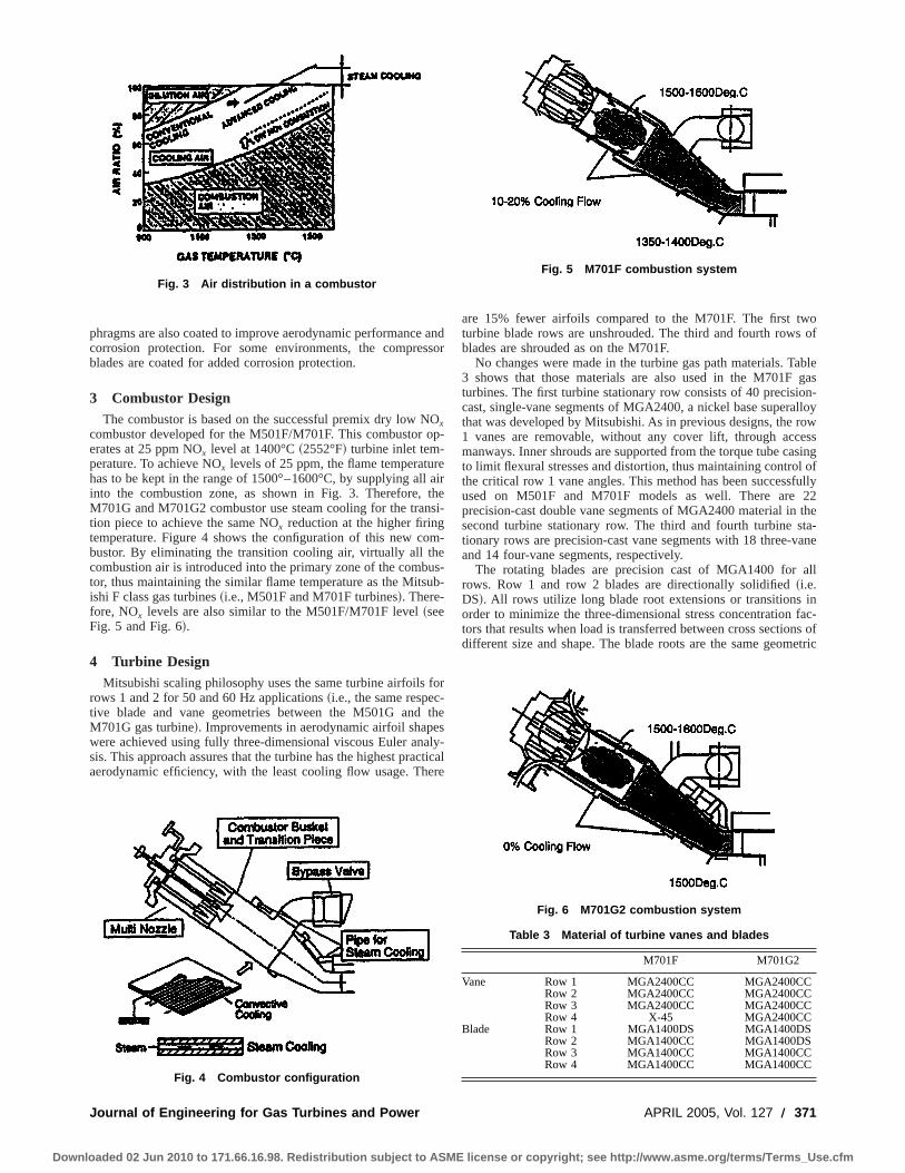
phragms are also coated to improve aerodynamic performance andcorrosion protection. For some environments, the compressorblades are coated for added corrosion protection.

3 Combustor DesignThe combustor is based on the successful premix dry low NOx

combustor developed for the M501F/M701F. This combustor op-erates at 25 ppm NOx level at 1400°C~2552°F! turbine inlet tem-perature. To achieve NOx levels of 25 ppm, the flame temperaturehas to be kept in the range of 1500°–1600°C, by supplying all airinto the combustion zone, as shown in Fig. 3. Therefore, theM701G and M701G2 combustor use steam cooling for the transi-tion piece to achieve the same NOx reduction at the higher firingtemperature. Figure 4 shows the configuration of this new com-bustor. By eliminating the transition cooling air, virtually all thecombustion air is introduced into the primary zone of the combus-tor, thus maintaining the similar flame temperature as the Mitsub-ishi F class gas turbines~i.e., M501F and M701F turbines!. There-fore, NOx levels are also similar to the M501F/M701F level~seeFig. 5 and Fig. 6!.

4 Turbine DesignMitsubishi scaling philosophy uses the same turbine airfoils for

rows 1 and 2 for 50 and 60 Hz applications~i.e., the same respec-tive blade and vane geometries between the M501G and theM701G gas turbine!. Improvements in aerodynamic airfoil shapeswere achieved using fully three-dimensional viscous Euler analy-sis. This approach assures that the turbine has the highest practicalaerodynamic efficiency, with the least cooling flow usage. There

are 15% fewer airfoils compared to the M701F. The first twoturbine blade rows are unshrouded. The third and fourth rows ofblades are shrouded as on the M701F.

No changes were made in the turbine gas path materials. Table3 shows that those materials are also used in the M701F gasturbines. The first turbine stationary row consists of 40 precision-cast, single-vane segments of MGA2400, a nickel base superalloythat was developed by Mitsubishi. As in previous designs, the row1 vanes are removable, without any cover lift, through accessmanways. Inner shrouds are supported from the torque tube casingto limit flexural stresses and distortion, thus maintaining control ofthe critical row 1 vane angles. This method has been successfullyused on M501F and M701F models as well. There are 22precision-cast double vane segments of MGA2400 material in thesecond turbine stationary row. The third and fourth turbine sta-tionary rows are precision-cast vane segments with 18 three-vaneand 14 four-vane segments, respectively.

The rotating blades are precision cast of MGA1400 for allrows. Row 1 and row 2 blades are directionally solidified~i.e.DS!. All rows utilize long blade root extensions or transitions inorder to minimize the three-dimensional stress concentration fac-tors that results when load is transferred between cross sections ofdifferent size and shape. The blade roots are the same geometric

Fig. 3 Air distribution in a combustor

Fig. 4 Combustor configuration

Fig. 5 M701F combustion system

Fig. 6 M701G2 combustion system

Table 3 Material of turbine vanes and blades

M701F M701G2

Vane Row 1 MGA2400CC MGA2400CCRow 2 MGA2400CC MGA2400CCRow 3 MGA2400CC MGA2400CCRow 4 X-45 MGA2400CC

Blade Row 1 MGA1400DS MGA1400DSRow 2 MGA1400CC MGA1400DSRow 3 MGA1400CC MGA1400CCRow 4 MGA1400CC MGA1400CC



multiple serration type used on past designs with four serrationsused on the first two rows and five serrations used on the last twostages.

Each row of vane segments is supported in a separate innercasing~blade ring! that is keyed and supported to permit radialand axial thermal response independent of possible external cyl-inder distortions. Blade ring distortion in the M701G~andM701G2! turbine is further minimized by the use of segmentedisolation rings that support the vane segments and also ring seg-ments over the rotor blades to form a thermal barrier between theflow path and the blade ring. As in all past designs, the interstageseal housings are uniquely supported from the inner shrouds ofrows 2, 3, and 4 vane segments by radial keys that permit thethermal response of the seal housings to be independent of themore rapid thermal response of the vane segments.

The row 1 vane cooling is provided by impingement, convec-tion and film cooling. The film cooling holes are fan shaped andboth the airfoil and shrouds will be coated with a ceramic thermalbarrier coating. The row 1 vane cooling design is shown in Fig. 7.This highly effective configuration utilizes state-of-the-art con-cepts with three impingement inserts in combination with an arrayof film cooling holes and a trailing edge pin fin system.

Film cooling is used at the leading edge as well as at selectedpressure and suction side locations. This limits vane wall thermalgradients and external surface temperatures.

Particular attention is paid to the inner and outer shrouds be-cause of the relatively flat temperature profile from the dry lowNOx combustor. Cooling of shrouds is provided by impingementplates and film cooling as well as convection cooling via drilledholes.

The row 1 blade cooling consists of convectional serpentinecooling with angled turbulators. The film cooling utilizes fanshaped cooling holes for more effective cooling. The blade also

features extensive film cooling at the tip to reduce the metal tem-perature of squealer tip and platform cooling holes to positivelycool the inner platforms. The airfoil is coated with a thermal bar-rier coating~Fig. 8!.

Blade and vane cooling flows have been kept to a minimumwhile maintaining similar metal surface temperatures, as in thecase of the M701F. These advanced turbine cooling schemes aredeveloped through heat transfer model tests and cooled turbine

Fig. 7 M701FG2 row 1 vane

Fig. 8 M701G2 row 1 blade

Fig. 9 Measurement of film cooling effectiveness in a lowspeed cascade

Fig. 10 Serpentine cooling passage test under rotation

Fig. 11 Measurement of airfoil heat transfer coefficient using aliquid crystal

Fig. 12 Hot cascade test



hot cascade tests. Those were also verified through a high-temperature demonstration unit by testing scaled-down turbineairfoils at the actual operating temperature. Figure 9 shows thefilm cooling test in a low-speed cascade to measure the film cool-ing effectiveness around the airfoil. Figure 10 shows the test ofserpentine cooling passage with a turbulence promoter to measurethe heat transfer characteristics under rotating conditions. Figure11 shows the airfoil heat transfer measurements using a liquidcrystal. Figure 12 shows the hot cascade test section. This cascadetest allows a measurement of airfoil cooling performance underactual firing conditions.

The row 2 vane is cooled by a combination of impingementcooling via the inserts and film cooling using fan shaped coolingholes. With the row 1 vane, intensive cooling schemes were de-veloped to the inner and outer shrouds using impingement andconvection cooling.

The row 2 blade is cooled by convection with no film cooling.The airfoil is coated with a thermal barrier coating. The row 3blade cooling is unique in that it positively cools the blade tip

Fig. 13 Startup hot gas type blade ring

Fig. 14 M701G2 factory load test condition

Fig. 15 Itemized measurement on M701G2

Fig. 16 Working compressor, stationary vane vibration stressmeasurement result



shroud. Because of the flatter~or relatively flat! profile from thecombustor, it was decided to allow for positive cooling of the tipshroud.

Compressor bleed air from the eighth stage is used to supplycooling air to the third-stage blade ring cavity. Cooling air isdirected to the inlet cavity of a five-cavity multipass convectivecooled vane airfoil. Leading edge cavity flow also supplies theinterstage seal and cooling system while the fifth pass cavity exitsthrough pressure side ‘‘holes’’ on the vane surface near the trailingedge. The fourth-stage vane is not cooled but does transport fifth-stage compressor bleed air for the fourth-row interstage seal andcooling system. The cooling system shown in Fig. 2 maintains theNiCrMoV turbine disk temperatures below 400°C~752 F!, whichensures the safe operation of the disks below the creep range,thereby assuring long service life.

The structure and the characteristic of the advanced blade ringare shown in Fig. 13. By means of steam, heating, the blade ring

is enlarged during start-up. During the rated load, the steam tem-perature is lower than the gas temperatures surrounding the bladering. This cools the blade ring, causing a relative contraction andestablishes the suitable clearance.

5 Factory Load Test of M701G2In order to confirm the performance and the reliability of the

M701G2, the factory load test was conducted in April and May2002. This load test facility is located at Mitsubishi Heavy Indus-tries Takasago Machinery Works. The factory load test facility isshown in Fig. 14. Over 1800 points were monitored with specialsensors, as shown in Fig. 15.

The test results confirmed that the performance, reliability, andstart-up characteristic of the compressor scaled accurately fromthe M501H gas turbine. In Fig. 16, the measured vibration stressof the compressor and the stationary vane are shown. The vibra-tion stress of the blade was measured by using optical fiber sensor.It was confirmed that the measured vibration stress is lower thanthe allowable value ensuring reliability. As shown in Fig. 17, itwas confirmed that gas turbine axial vibration was extremely low.

The tests confirmed the overall performance capability and re-liability of the M701G2 gas turbine.

6 ConclusionThe M701G2 successfully incorporates M501H gas turbine

technology without changing hot gas path materials or rotor ma-terials and without shifting to steam cooling for the turbine bladesand vanes. The output and heat rates are almost equivalent to thatof H technology. The factory load tests of the M701G2 were con-ducted in April 2002 by monitoring over 1800 points with specialsensors and confirmed that high mechanical reliability is achiev-able.

References@1# Aoki, S., ‘‘Trend and Key Technologies for Gas Turbine Combined Cycle

Power Generation in a Globally Competitive Market and Environmental Regu-lations,’’ IJPGC2000-15084, 2000.

@2# Koeneke, C., Kallianpur, V., Arimura, H. et al., ‘‘Maintaining Long TermSteam Cooling Reliability in Mitsubishi Advanced Industrial Gas Turbines:Approach, Technology & Field Experience,’’ PowerGen 2002.

Fig. 17 Rotor vibration measurement result



Gary D. Lock

Youyou Yan1

Paul J. Newton

Michael Wilson

J. Michael Owen

Department of Mechanical Engineering,University of Bath,Bath BA2 7AY, UK

Heat Transfer MeasurementsUsing Liquid Crystals in aPreswirl Rotating-Disk SystemPreswirl nozzles are often used in gas turbines to deliver the cooling air to the turbineblades through receiver holes in a rotating disk. The distribution of the local Nusseltnumber, Nu, on the rotating disk is governed by three nondimensional fluid-dynamicparameters: preswirl ratio,bp , rotational Reynolds number, Ref , and turbulent flowparameter,lT . A scaled model of a gas turbine rotor–stator cavity, based on the geom-etry of current engine designs, has been used to create appropriate flow conditions. Thispaper describes how a thermochromic liquid crystal, in conjunction with a stroboscopiclight and digital camera, is used in a transient experiment to obtain contour maps of Nuon the rotating disk. The thermal boundary conditions for the transient technique are suchthat an exponential-series solution to Fourier’s one-dimensional conduction equation isnecessary. A method to assess the uncertainty in the measurements is discussed and theseuncertainties are quantified. The experiments reveal that Nu on the rotating disk is axi-symmetric except in the region of the receiver holes, where significant two-dimensionalvariations have been measured. At the higher coolant flow rates studied, there is a peak inheat transfer at the radius of the preswirl nozzles. The heat transfer is governed by twoflow regimes: one dominated by inertial effects associated with the impinging jets from thepreswirl nozzles, and another dominated by viscous effects at lower flow rates. The Nus-selt number is observed to increase as either Ref or lT increases.@DOI: 10.1115/1.1787509#

1 Introduction

Preswirl nozzles are often used in gas turbines to deliver thecooling air to the turbine blades, as illustrated in Fig. 1. The sta-tionary nozzles swirl the cooling air in the direction of rotation ofthe turbine disk, thereby reducing the temperature of the air rela-tive to the blades. The designer needs to know the effect of thepreswirl ratio,bp , the coolant flow rate, and the rotational speed,V, on the pressure drop and temperature difference between thepreswirl nozzles and the receiver holes in the disk. It is also im-portant to know the effect of these parameters on the distributionof Nusselt number, Nu, over the surface of the rotating disk.

Owen and Rogers@1# described early studies of preswirl sys-tems, and Owen and Wilson@2# gave a brief review of morerecent heat transfer research. Metzger, Bunker, and Bosch@3#were the first to apply a thermochromic liquid crystal to the caseof a rotating disk with jet impingement. Karabay, Wilson, andOwen@4# carried out a combined experimental and computationalstudy of flow in a ‘‘cover-plate’’~rotating cavity! preswirl system.A theoretical analysis was used to show that there was an optimalvalue of the preswirl ratio, for which the average Nusselt numberfor a heated rotating disk would be a minimum. Pilbrow et al.@5#presented experimental and computational results for heat transferin the same cover-plate system, showing that the structure of theseflows is governed principally by the values ofbp , and theturbulent-flow parameter,lT . For a detailed discussion of thesignificance oflT , the reader is referred to Ref.@1#. The heat

transfer is governed by the above two parameters as well as by therotational Reynolds number, Ref , and by the temperature distri-bution on the rotating disk.

Designers can obtain some information using turbine-based rigsrunning close to engine-operating conditions. However, deeper in-sight can be gained from fundamental research that measures,computes, and explains the flow and heat transfer in generic, fullyinstrumented rigs operating under more benign conditions. Com-putational codes, validated on these detailed measurements,can then be used to conduct calculations extrapolated to engineconditions.

This paper describes a generic rig, which has been constructedto study the fluid dynamics and heat transfer in preswirl systems.The experimental facility is a simplified model of a gas turbinerotor–stator system designed to accommodate pressure and tem-perature instrumentation in the test section and to provide opticalaccess to the wheel space. The fluid dynamics has been investi-gated both experimentally and computationally by Yan et al.@6#.The effects of rotational speed, flow rate, preswirl ratio, and thenumber of preswirl nozzles on the flow field and on the totalpressure losses in the system have been reported. These measure-ments and computations showed that there was a significant lossof total pressure between the outlet from the preswirl nozzles andthe rotating core of fluid in the wheel space. This loss increased asthe preswirl flow rate and inlet swirl ratio increased, and as thenumber of nozzles decreased. The discharge coefficient of thereceiver holes increased as the swirl ratio at the receiver-holeradius approached unity.

The complementary measurements of heat transfer using ther-mochromic liquid crystals~TLCs! are discussed here, featuringthe novel technique of stroboscopic lighting and an exponential-series solution to Fourier’s conduction equation. Contour maps ofNu on the rotating disk have been measured, including detailedtwo-dimensional patterns around the blade receiver holes. Al-

1Present address: City University, London, Northampton Square, London EC1V0HB, U.K.




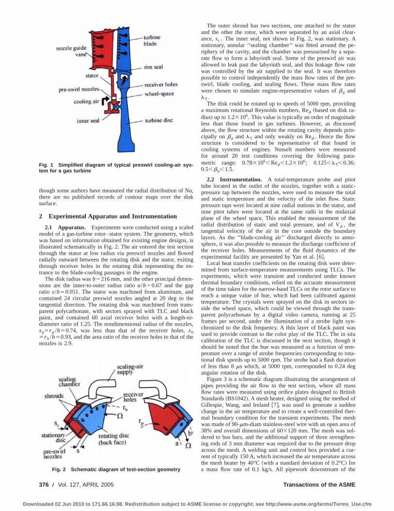
though some authors have measured the radial distribution of Nu,there are no published records of contour maps over the disksurface.

2 Experimental Apparatus and Instrumentation

2.1 Apparatus. Experiments were conducted using a scaledmodel of a gas-turbine rotor–stator system. The geometry, whichwas based on information obtained for existing engine designs, isillustrated schematically in Fig. 2. The air entered the test sectionthrough the stator at low radius via preswirl nozzles and flowedradially outward between the rotating disk and the stator, exitingthrough receiver holes in the rotating disk representing the en-trance to the blade-cooling passages in the engine.

The disk radius wasb5216 mm, and the other principal dimen-sions are the inner-to-outer radius ratioa/b50.67 and the gapratio s/b50.051. The stator was machined from aluminum, andcontained 24 circular preswirl nozzles angled at 20 deg to thetangential direction. The rotating disk was machined from trans-parent polycarbonate, with sectors sprayed with TLC and blackpaint, and contained 60 axial receiver holes with a length-to-diameter ratio of 1.25. The nondimensional radius of the nozzles,xp5r p /b50.74, was less than that of the receiver holes,xb5r b /b50.93, and the area ratio of the receiver holes to that of thenozzles is 2.9.

The outer shroud has two sections, one attached to the statorand the other the rotor, which were separated by an axial clear-ance,sc . The inner seal, not shown in Fig. 2, was stationary. Astationary, annular ‘‘sealing chamber’’ was fitted around the pe-riphery of the cavity, and the chamber was pressurised by a sepa-rate flow to form a labyrinth seal. Some of the preswirl air wasallowed to leak past the labyrinth seal, and this leakage flow ratewas controlled by the air supplied to the seal. It was thereforepossible to control independently the mass flow rates of the pre-swirl, blade cooling, and sealing flows. These mass flow rateswere chosen to simulate engine-representative values ofbp andlT .

The disk could be rotated up to speeds of 5000 rpm, providinga maximum rotational Reynolds numbers, Ref ~based on disk ra-dius! up to 1.23106. This value is typically an order of magnitudeless than those found in gas turbines. However, as discussedabove, the flow structure within the rotating cavity depends prin-cipally on bp and lT and only weakly on Ref . Hence the flowstructure is considered to be representative of that found incooling systems of engines. Nusselt numbers were measuredfor around 20 test conditions covering the following para-metric range: 0.783106,Ref,1.23106; 0.125,lT,0.36;0.5,bp,1.5.

2.2 Instrumentation. A total-temperature probe and pitottube located in the outlet of the nozzles, together with a static-pressure tap between the nozzles, were used to measure the totaland static temperature and the velocity of the inlet flow. Staticpressure taps were located at nine radial stations in the stator, andnine pitot tubes were located at the same radii in the midaxialplane of the wheel space. This enabled the measurement of theradial distribution of static and total pressure, and ofVf , thetangential velocity of the air in the core outside the boundarylayers. As the ‘‘blade-cooling air’’ discharged directly to atmo-sphere, it was also possible to measure the discharge coefficient ofthe receiver holes. Measurements of the fluid dynamics of theexperimental facility are presented by Yan et al.@6#.

Local heat transfer coefficients on the rotating disk were deter-mined from surface-temperature measurements using TLCs. Theexperiments, which were transient and conducted under knownthermal boundary conditions, relied on the accurate measurementof the time taken for the narrow-band TLCs on the rotor surface toreach a unique value of hue, which had been calibrated againsttemperature. The crystals were sprayed on the disk in sectors in-side the wheel space, which could be viewed through the trans-parent polycarbonate by a digital video camera, running at 25frames per second, under the illumination of a strobe light syn-chronized to the disk frequency. A thin layer of black paint wasused to provide contrast to the color play of the TLC. The in situcalibration of the TLC is discussed in the next section, though itshould be noted that the hue was measured as a function of tem-perature over a range of strobe frequencies corresponding to rota-tional disk speeds up to 5000 rpm. The strobe had a flash durationof less than 8ms which, at 5000 rpm, corresponded to 0.24 degangular rotation of the disk.

Figure 3 is a schematic diagram illustrating the arrangement ofpipes providing the air flow to the test section, where all massflow rates were measured using orifice plates designed to BritishStandards~BS1042!. A mesh heater, designed using the method ofGillespie, Wang, and Ireland@7#, was used to generate a suddenchange in the air temperature and to create a well-controlled ther-mal boundary condition for the transient experiments. The meshwas made of 90-mm-diam stainless-steel wire with an open area of38% and overall dimensions of 603120 mm. The mesh was sol-dered to bus bars, and the additional support of three strengthen-ing rods of 3 mm diameter was required due to the pressure dropacross the mesh. A welding unit and control box provided a cur-rent of typically 150 A, which increased the air temperature acrossthe mesh heater by 40°C~with a standard deviation of 0.2°C! fora mass flow rate of 0.1 kg/s. All pipework downstream of the

Fig. 1 Simplified diagram of typical preswirl cooling-air sys-tem for a gas turbine

Fig. 2 Schematic diagram of test-section geometry



mesh heater was thermally insulated using low-conductivityRhoacell, a closed-pore structural foam with low thermal conduc-tivity. This pipework had three main components: a 350-mmlength of rectangular cross section, a 350-mm length of circularcross section, and a radial diffuser; there was also a short entrylength into the preswirl nozzles. The temperature history of the airleaving the preswirl nozzles is described in Sec. 3.

Before the main mesh heater was switched on, the apparatuswas left running, at the required speed and flow rate, to enable itto reach thermal equilibrium. When the air from the compressorwas not equal to the ambient temperature in the laboratory, it waseither cooled by a heat exchanger or heated by a second meshheater upstream of the main heater. In practice, it was not possibleto achieve perfect thermal equilibrium, and there was always asmall temperature difference between the rotating disk and the air,as discussed in Sec. 4.

3 Temperature Measurement

3.1 Total-Temperature Probes. A conventional total-temperature probe usually contains a thermocouple, the bead ofwhich is located inside a stainless-steel tube. Such probes have alarge recovery factor~'0.95! but a poor time response. For thetests described here, a K-type bare-wire thermocouple, made fromwires of 25mm diameter, was constructed. The wires were con-tained inside a stainless steel tube with the bead outside; there wasa distance of 3.5 mm~or 140 wire diameters! between the exposedbead and the tip of the tube. This construction method supportedthe thermocouple wires but reduced the thermal error resultingfrom transient conduction from the bead to the tube. The resultwas a robust probe with a time constant of less than 40 ms. Aconsistent probe recovery factor of 0.78 was measured over arange of air speeds up to 120 m/s.

Figure 4 shows a typical increase in air temperature with timemeasured by the probe immediately downstream of the meshheater and at the outlet of the preswirl nozzles. Downstream of theheater there is a good approximation to a step change. Owing tothe thermal inertia of the ducting between the heater and the testsection, a step change is not produced at the nozzles; it can beseen that a good fit to the temperature is provided by an exponen-tial series ofm53 terms~see Sec. 4.2!. It seems likely that threeterms are required in the exponential fit because there are threedistinct geometric sections to the duct downstream of the heatermesh, as discussed above. Typically the TLC color-change timeson the disk surface ranged between 1 and 20 s~depending on thelocal heat transfer coefficient!, and these times are of similarmagnitude to the time constants of the exponential rise in airtemperature.

3.2 Calibration of TLCs. Microencapsulated TLCs werepurchased commercially in the form of a water-based slurry. Threetypes of TLC were used: two narrow-band crystals optically active

over a temperature range of around 1°C near 30°C~R30C1W! and40°C ~R40C1W!, and one wide-band crystal~R18C20W! activefrom approximately 18°C over a 20°C range.

The crystals were calibrated against temperature by recordingthe red, green, and blue~RGB! signals of light reflected from theTLC, under known temperature and illumination, using a digitalcamera, an isothermal copper block, and an AGEMA 870Cinfrared-imager@8#. The RGB signals were converted into hues,which increase monotonically with temperature.

The TLC was applied to the rotor surface using an airbrush, andblack paint was sprayed on top of the TLC to provide contrast tothe color play from the crystals. The overall thickness~TLC andpaint! was approximately 25mm. During the experiments the TLCwas viewed through the transparent polycarbonate disk using thestroboscopic light synchronized to the rotational speed of the disk.For the calibration, the stator was removed to gain direct opticalaccess to the front surface of the disk, which was coated in TLCunder black paint and heated quasiaxisymmetrically by a jet of hotair. The surface temperature of the front face was measured usingan infrared imager. The back face of the disk was simultaneouslyilluminated by the stroboscopic light and the TLC was viewed bythe digital camera, located behind the disk. The locations of thestroboscopic light and camera were the same as those used in theexperiments, creating an in situ calibration.

It has been shown@8,9# that rotational speed has no significanteffect on the calibration of TLCs, and so the calibrations wereconducted with the disk stationary. To ensure that the strobe fre-quency had no effect, calibrations were carried out for frequenciescorresponding to 3000, 4000, and 5000 rpm.

Figure 5 shows the calibrated variation of temperature with

Fig. 3 Schematic layout of experiment

Fig. 4 Increase in air temperature with time measured at twolocations; a fitted curve is also shown for mÄ3

Fig. 5 Calibrated temperature versus normalized hue for threecrystals at three strobe frequencies



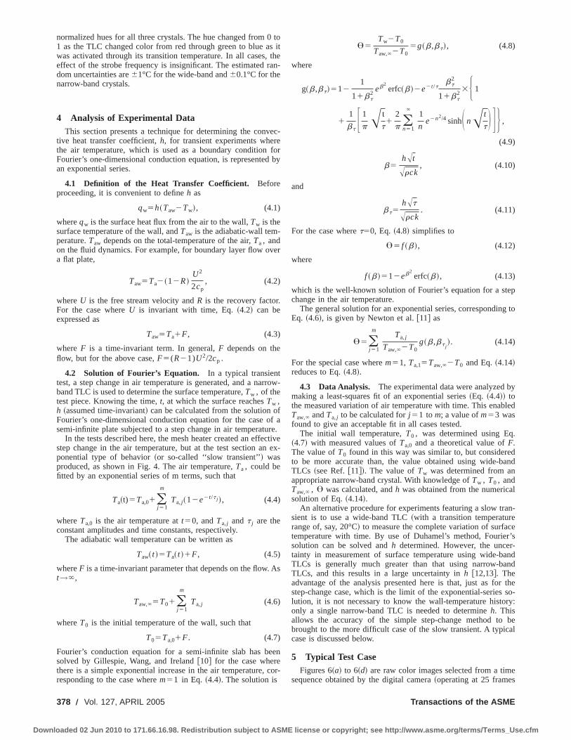
normalized hues for all three crystals. The hue changed from 0 to1 as the TLC changed color from red through green to blue as itwas activated through its transition temperature. In all cases, theeffect of the strobe frequency is insignificant. The estimated ran-dom uncertainties are61°C for the wide-band and60.1°C for thenarrow-band crystals.

4 Analysis of Experimental DataThis section presents a technique for determining the convec-

tive heat transfer coefficient,h, for transient experiments wherethe air temperature, which is used as a boundary condition forFourier’s one-dimensional conduction equation, is represented byan exponential series.

4.1 Definition of the Heat Transfer Coefficient. Beforeproceeding, it is convenient to defineh as

qw5h~Taw2Tw!, (4.1)

whereqw is the surface heat flux from the air to the wall,Tw is thesurface temperature of the wall, andTaw is the adiabatic-wall tem-perature.Taw depends on the total-temperature of the air,Ta, andon the fluid dynamics. For example, for boundary layer flow overa flat plate,

Taw5Ta2~12R!U2

2cp, (4.2)

whereU is the free stream velocity andR is the recovery factor.For the case whereU is invariant with time, Eq.~4.2! can beexpressed as

Taw5Ta1F, (4.3)

where F is a time-invariant term. In general,F depends on theflow, but for the above case,F5(R21)U2/2cp .

4.2 Solution of Fourier’s Equation. In a typical transienttest, a step change in air temperature is generated, and a narrow-band TLC is used to determine the surface temperature,Tw , of thetest piece. Knowing the time,t, at which the surface reachesTw ,h ~assumed time-invariant! can be calculated from the solution ofFourier’s one-dimensional conduction equation for the case of asemi-infinite plate subjected to a step change in air temperature.

In the tests described here, the mesh heater created an effectivestep change in the air temperature, but at the test section an ex-ponential type of behavior~or so-called ‘‘slow transient’’! wasproduced, as shown in Fig. 4. The air temperature,Ta, could befitted by an exponential series of m terms, such that

Ta~t)5Ta,01(j 51

m

Ta,j~12e2t/t j !, (4.4)

whereTa,0 is the air temperature att50, andTa,j and t j are theconstant amplitudes and time constants, respectively.

The adiabatic wall temperature can be written as

Taw~ t !5Ta~ t !1F, (4.5)

whereF is a time-invariant parameter that depends on the flow. Ast→`,

Taw, 5T01(j 51

m

Ta,j (4.6)

whereT0 is the initial temperature of the wall, such that

T05Ta,01F. (4.7)

Fourier’s conduction equation for a semi-infinite slab has beensolved by Gillespie, Wang, and Ireland@10# for the case wherethere is a simple exponential increase in the air temperature, cor-responding to the case wherem51 in Eq. ~4.4!. The solution is

U5Tw2T0

Taw, 2T05g~b,bt!, (4.8)

where

g~b,bt!5121

11bt2

eb2erfc~b!2e2t/t

bt2

11bt2

3H 1

11

btF 1

pA t

t1

2

p (n51

`1

ne2n2/4 sinhS nAt

t D G J ,

(4.9)

b5hAt

Arck, (4.10)

and

bt5hAt

Arck. (4.11)

For the case wheret50, Eq. ~4.8! simplifies to

U5 f ~b!, (4.12)

where

f ~b!512eb2erfc~b!, (4.13)

which is the well-known solution of Fourier’s equation for a stepchange in the air temperature.

The general solution for an exponential series, corresponding toEq. ~4.6!, is given by Newton et al.@11# as

U5(j 51

mTa,j

Taw, 2T0g~b,bt j

!. (4.14)

For the special case wherem51, Ta,15Taw, 2T0 and Eq.~4.14!reduces to Eq.~4.8!.

4.3 Data Analysis. The experimental data were analyzed bymaking a least-squares fit of an exponential series~Eq. ~4.4!! tothe measured variation of air temperature with time. This enabledTaw, andTa,j to be calculated forj 51 to m; a value ofm53 wasfound to give an acceptable fit in all cases tested.

The initial wall temperature,T0 , was determined using Eq.~4.7! with measured values ofTa,0 and a theoretical value ofF.The value ofT0 found in this way was similar to, but consideredto be more accurate than, the value obtained using wide-bandTLCs ~see Ref.@11#!. The value ofTw was determined from anappropriate narrow-band crystal. With knowledge ofTw , T0 , andTaw, , U was calculated, andh was obtained from the numericalsolution of Eq.~4.14!.

An alternative procedure for experiments featuring a slow tran-sient is to use a wide-band TLC~with a transition temperaturerange of, say, 20°C! to measure the complete variation of surfacetemperature with time. By use of Duhamel’s method, Fourier’ssolution can be solved andh determined. However, the uncer-tainty in measurement of surface temperature using wide-bandTLCs is generally much greater than that using narrow-bandTLCs, and this results in a large uncertainty inh @12,13#. Theadvantage of the analysis presented here is that, just as for thestep-change case, which is the limit of the exponential-series so-lution, it is not necessary to know the wall-temperature history:only a single narrow-band TLC is needed to determineh. Thisallows the accuracy of the simple step-change method to bebrought to the more difficult case of the slow transient. A typicalcase is discussed below.

5 Typical Test CaseFigures 6~a! to 6~d! are raw color images selected from a time

sequence obtained by the digital camera~operating at 25 frames



per second! during a typical experiment. These images show thecolor play of the TLC as viewed through the transparent polycar-bonate disk. Initially clear when below its activation temperature,the TLC changed color from red to green to blue as the disk was

heated by the hot gas entering through the preswirl nozzles. Theimages appear ‘‘frozen’’ because the rotor was illuminated by thestroboscopic light synchronized with the disk rotating at 5000rpm.

A color version of Fig. 6~and Figs. 7 and 8! appear in ASMEpaper GT-2003-38123. The hub and casing, at radiia and b, aremarked in Fig. 6~a!. The blade receiver holes, insulated usinglow-conductivity, white-colored Rhoacell foam, are also labeled.The narrow-band TLC and overcoat of black paint had beensprayed in a 48 deg sector on the disk covering 8 of the 60 re-ceiver holes. To the left of this painted sector the stator, coatedwith a wide-band~initially red! TLC, and two of the 24 preswirlnozzles are visible through the transparent~unpainted! polycar-bonate at low radius. Some shadows appear around the receiverholes due to constraints with the lighting and viewing angles.

In Fig. 6~a! the 30°C narrow-band TLC has been activated intoits visible range~shown as blue! near the blade receiver holes.Elsewhere on the disk the TLC is still clear~showing black!,indicating that there is a region of relatively high heat transferaround the holes. The virtually identical TLC patterns around eachof the receiver holes clearly indicate the excellent periodicity ofthe flow structure. In Figs. 6~b! and 6~c!, the 30°C crystal hasbeen activated~green and blue, respectively! at radii between thepreswirl nozzles and the receiver holes. In Fig. 6~c! the 40°C TLChas been activated by temperature~light blue! in the region aroundthe receiver holes and has turned dark blue in Fig. 6~d!. The 40°CTLC is activated at lower radii in Fig. 6~d! ~red-green!. Note thatthe stator, as indicated by the change in color of the wide-bandTLC, has also been heated throughout this transient process.

These RGB images~of 8003600 pixels!, recorded at 25 framesper second by the digital camera, were subsequently converted tohues on a PC. It was then possible to obtain the hue history ofeach pixel in the image and hence the time taken for the surface toreach a prescribed value of hue. Thus the time taken for the sur-face to reach the temperature of the calibrated narrow-band crys-tal, Tw , from an initial temperature,T0 , was measured at eachpixel on the active surface of the disk in the field-of-view of thecamera. A ‘‘median filter,’’ using the median of nine adjacent pix-els, was used to reduce the uncertainty in the measured values ofTw .

6 Nusselt NumberFigure 7 shows contours of the measured Nusselt number on

the rotating disk for Ref50.83106, lT'0.125, andbp'0.5; thedirection of rotation of the disk is clockwise. The distribution ofNu is largely axisymmetric, except in the region around the re-

Fig. 6 a–d „top to bottom … Video recordings of disk surfaceshowing change of color of TLC with time

Fig. 7 Contours of Nu: Re fÉ0.8Ã106, lTÉ0.125, bpÉ0.5; thedisk is rotating clockwise



ceiver holes. The highest heat transfer rates occur between theholes, and there is repeatability in both magnitudes and the varia-tions of Nu between successive holes.

Figures 8~a! and 8~b! show contours of Nu for a higher flowrate,lT'0.36,bp'1.4, for Ref50.83106 and Ref51.183106,respectively. The color scales have been chosen independently inorder to show clearly the variations around the receiver holes.Comparing Fig. 4 and Fig. 5~a!, for which Ref50.83106 in bothcases, there is higher heat transfer around the preswirl nozzleradius,xp50.74, at the higher flow rate. There are similar varia-tions ~and similarly good repeatability of results! between the re-ceiver holes on the disk; Nu is also higher in this region for thehigher flow rate case. Figures 8~a! and 8~b! show that Nu in-creases generally with increasing Ref .

6.1 Effect of Ref on Radial Variation of Nu. The varia-tions of Nu with the parameterslT and bp , and with Ref , arebest observed by using results taken along a radial line midwaybetween receiver holes. Figure 9 shows the effect of Ref on themeasured radial variation of Nusselt number at two fixed values oflT ~0.125 and 0.36 approximately!, for which bp'0.5 and 1.4,respectively. For each fixed value oflT ~andbp), the magnitudeof Nu increases with increasing Ref , but there is little effect ofRef on theshapeof the Nu distributions. For all cases, there is apeak in measured values of Nu in the region near the receiverholes on the disk. Figure 9~a! (lT'0.125,bp'0.5) shows that Nuincreases with radius between the preswirl nozzle radius,xp

50.74, and the receiver holes. This behavior is similar, qualita-tively, to heat transfer in a simple rotor–stator system with a radialoutflow @14#, suggesting that heat transfer is controlled mainly bythe boundary-layer flow on the rotating disk. Forx.0.9, there isa rapid rise in measured Nu. In this region, disk boundary layerfluid enters the receiver holes and there is strong flow axiallytoward the disk, causing an increase in heat transfer.

Figure 9b shows that forlT'0.36 (bp'1.4) a local peak in Nuoccurs around the nozzle radiusxp , and Nu decreases forxp,x,xb . This suggests that inertial ‘‘impingement’’ effects have amore significant influence, due to the more powerful preswirl flowat this higher value oflT , than for the cases in Fig. 9~a!.

6.2 Effect of lT and bp on the Radial Variation ofNu. Figures 9~a! and 9~b! also show, respectively, the effect ofvarying lT ~and, as a consequence, varyingbp) on the measuredradial variation of Nu for Ref'0.83106 ~blue circles! and 1.23106 ~red triangles!. At both values of Ref , there is a similartransition in the variation of Nu withx, from the viscous behaviordescribed above forlT'0.125 (bp'0.5) to inertial behavior forlT'0.36 (bp'1.4).

The combined effect of increasinglT and bp at fixed Ref isgreatest for x,0.9, approximately. There is less sensitivity tolTand bp for the region around and outward of the receiver holes,and this sensitivity also tends to decrease as Ref increases.

6.3 Use of Two Crystals. The method of analysis describedin Sec. 4 only requires a measurement of a single narrow-bandTLC. Two narrow-band TLCs were used to test the accuracy ofthe measurements. Figure 10 showsh, rather than Nu, again mea-sured along a radius midway between two receiver holes for theviscous and inertial cases discussed above. Data from both the 30and 40°C TLCs are shown.

There is good agreement between the data collected from thetwo TLCs for the viscous case. However, in the inertial case,hmeasured using the 40°C crystal is consistently higher than thatobtained using the 30°C crystal. These cases are typical examplesfrom a range of experimental data. Before discussing possiblereasons for differences in the measurements ofh, it is necessary toconsider the uncertainties in these measurements.

The uncertainty analysis described by Owen, Newton, and Lock@13# was used to create the ‘‘uncertainty bars’’ shown in Fig. 10.Small, random uncertainties in the measured temperature can pro-duce large uncertainties in the calculated values ofh. If PTw

, PT0,

Fig. 8 Effect of Re f on contours Nu for lTÉ0.36 and bpÉ1.4:„a… RefÉ0.8Ã106, „b… RefÉ1.18Ã106; the disk is rotating clock-wise

Fig. 9 Effect of Re f on radial variation of Nu „a… lTÉ0.125,bpÉ0.52; „b… lTÉ0.36, bpÉ1.4 RefÉ0.8Ã106 d RefÉ1.2Ã106 .



andPTaware the relative uncertainties~95% confidence estimates!

in Tw , T0 andTaw, respectively, thenPh , the relative uncertaintyin h, can be determined from

Ph

h5Fh

PT

Taw2T0, (6.1)

where Fh is the so-calledamplification parameterand PT5max(PTw

,PT0,PTaw

).The uncertainty bars in Fig. 10 are based on a 0.2°C tempera-

ture uncertainty. Despite the random uncertainties, there is no evi-dence of significant scatter in the results. The ‘‘smoothness’’ of thedistribution ofh is attributed to the smoothing of the air tempera-ture and to the median filtering used for the wall temperatures.

There are three suspected reasons for the differences in themeasurements ofh from the two crystals:~i! incorrect values ofTaw; ~ii ! incorrect values ofT0 ; ~iii ! effect of radial distributionof Tw .

~i! Taw, given by Eq.~4.5!, depends onTa, the local tempera-ture in the fluid core. Unfortunately this temperature was not mea-sured in the experiments but was assumed to be equal to themeasured temperature at exit from the preswirl nozzles. It isspeculated that, as heat flows from the air to the rotating disk, thetemperature of the fluid in the core, and henceTaw, will be lessthan Ta. Consequently the value ofTaw given by Eq.~4.2! willoverestimate the true value, which in turn would cause an under-estimate in the true value ofh. The values ofh calculated from the40°C crystal should, by this argument, be closer to the true valuesthan those from the 30°C crystal. This uncertainty inTa wouldhave a more significant in the inertial regime than the viscousregime; in the former there is relatively high heat transfer andmore mixing of air between the core and the region near the wall.

~ii ! There is an uncertainty in the value ofT0 and this couldbias the calculated values ofh. A bias in T0 would qualitativelyaffect both measurements ofh in the same way, though not in aquantitatively equal manner.

~iii ! As discussed by Butler and Baughn@15#, the distributionof h is affected by the distribution ofTw . This effect is particu-larly significant in rotating-disk systems@1# where the radial dis-tribution of h depends strongly on the radial gradient of disk tem-perature. As the radial distributions ofTw are, perforce, differentfor the two crystals, it is reasonable to speculate that the radialdistribution ofh will be different. In addition, in regions of highlocal temperature gradients there is an effect of lateral conductionwhich can cause an overestimate in the value ofh from one-dimensional conduction analysis@16#. This error has not beenquantified here.

The fact that differences inh, albeit within the limits of experi-mental uncertainty, could be measured is a tribute to the

exponential-series technique and to the careful calibration of theTLCs. These measurements also reveal the benefits of using twocrystals to evaluateh: one crystal would only provide the bliss ofignorance!

The measurements ofh obtained using the 40°C crystal areconsidered more accurate than those obtained using the 30°Ccrystal. All data in Figs. 7–9 are based on the 40°C crystal.

7 ConclusionsAn experimental facility has been built to investigate the heat

transfer and fluid dynamics of a rotor–stator system with pre-swirled air under engine-representative flow structure. The facilityhas been designed to accommodate pressure and temperature in-strumentation in the test section and to provide optical access tothe wheel space.

A thermochromic liquid crystal~TLC!, in conjunction with astroboscopic light and digital video camera, has been used to ob-tain contour maps of the Nusselt number, Nu, on the rotating disk.Both wide-band and narrow-band TLCs were used and carefullycalibratedin situ using an infrared imager.

A mesh heater was used to generate an air temperature historyin the test section, which was represented as an exponential seriesof three terms. An analysis has been developed to determine val-ues of Nu by using this series as a boundary condition for Fouri-er’s one-dimensional conduction equation. This technique has theadvantage, in terms of accuracy and simplicity, that only a singlenarrow-band TLC is needed to determineh.

Two heat transfer regimes were observed experimentally: a vis-cous regime at relatively low values oflT , and an inertial regimeat high values oflT . The viscous regime corresponds to axisym-metric boundary layer flow over most of the rotating disk: forx,xb , Nu increases asx increases. Three-dimensional flow nearthe receiver holes on the disk, atx5xb , creates nonaxisymmetricflow in this region, with large values of Nu between and aroundthe holes. The inertial regime corresponds to impingement on therotating disk around the preswirl nozzle radius,x5xp . There is apeak in Nu nearx5xp and, for xp,x,xb , Nu decreases asxincreases; this behavior is also virtually axisymmetric. As for theviscous regime, there are large values and two-dimensional varia-tions of Nu around the receiver holes. For both regimes, Nu in-creases as Ref , lT , andbp increase.

AcknowledgmentThis work was funded by Alstom Power, Ltd. and the U.K.

EPSRC.

Nomenclature

a 5 inner radius of the diskb 5 outer radius of the diskc 5 specific heat of wall

cp 5 specific heat at constant pressure of airCw 5 nondimensional mass flow rate (5m/mb)

f (b) 5 step-change solution of Fourier’s equationF 5 time-invariant adiabatic-wall parameter (5Taw2Ta)

g(b,bt)5 exponential solution of Fourier’s equationh 5 heat transfer coefficient@5qw /(Taw2Tw)#k 5 thermal conductivity of wall

m 5 number of terms in exponential seriesNu 5 Nusselt number@5qwr /k(Taw2Tw)#

P 5 uncertainty in measured valueqw 5 heat flux from air to wall

r 5 radius from axis of rotationR 5 recovery factor

Ref 5 rotational Reynolds number (5rVb2/m)s 5 gap width

sc 5 clearance spacingt 5 time

T 5 temperature inside wall

Fig. 10 Heat transfer coefficient versus normalized radius forviscous and inertial flows. m Viscous—H40; d Inertial—H40; mViscous—H30; d Inertial—H30. „h uncertainty for 0.2°C tem-perature uncertainty. …



Ta 5 total temperature of airTaw 5 adiabatic-wall temperatureTw 5 surface temperature of wallU 5 free-stream velocity

Vf 5 tangential component of velocityx 5 nondimensional radius (5r /b)a 5 thermal diffusivity of wall (5k/rc)b 5 parameter in step-change solution (5hAt/rck)

bp 5 preswirl ratio (5Vf,p /Vr p)bt 5 parameter in exponential solution (5hAt/rck)lT 5 turbulent flow parameter (5Cw,p /Ref

0.8)r 5 densityU 5 nondimensional temperature@5(Tw2T0)/(Taw,

2T0)#F 5 amplification parameter for uncertaintiesm 5 dynamic viscosityV 5 angular speed of rotating diskt 5 time constant

Subscripts

h 5 with reference to heat transfer coefficientj 5 jth term in series

T 5 with reference to maximum value ofPTw, PT0

, andPTaw

Taw 5 with reference to adiabatic wall temperatureT0 5 with reference to initial temperatureTw 5 with reference to surface temperature

p 5 preswirl nozzle0 5 value att50` 5 value ast→`

References@1# Owen, J. M., and Rogers, R. H., 1989,Flow and Heat Transfer in Rotating

Disc Systems: Vol. 1, Rotor-Stator Systems, Research Studies Press, Taunton,UK and Wiley, NY.

@2# Owen, J. M., and Wilson, M., 2000, ‘‘Some Current Research in Rotating-DiscSystems,’’ in Turbine 2000 Int. Symp. on Heat Transfer in Gas Turbine Sys-tems, Turkey, August 13–18, in Heat Transfer in Gas Turbine Systems, Annalsof the New York Academy of Sciences,934, pp. 206–221.

@3# Metzger, D. E., Bunker, R. S., and Bosch, G., 1991, ‘‘Transient Liquid CrystalMeasurement of Local Heat Transfer on a Rotating Disk With Jet Impinge-ment,’’ ASME J. Turbomach.,113, pp. 52–59.

@4# Karabay, H., Wilson, M., and Owen, J. M., 2001, ‘‘Predictions of Effect ofSwirl on Flow and Heat Transfer in a Rotating Cavity,’’ Int. J. Heat Fluid Flow,22, pp. 143–155.

@5# Pilbrow, R., Karabay, H., Wilson, M., and Owen, J. M., 1999, ‘‘Heat Transferin a ‘Cover-Plate’ Pre-Swirl Rotating-Disc System,’’ ASME J. Turbomach.,121, pp. 249–256.

@6# Yan, Y., Gord, M. F., Lock, G. D., Wilson, M., and Owen, J. M., 2002, Fluiddynamics of a pre-swirl rotating-disk system, ASME paper 2002-GT-30415~tobe published in the J Turbomachinery!.

@7# Gillespie, D. R. H., Wang, Z., and Ireland, P. T., 2001, Heater element, Euro-pean Patent No. 0847679.

@8# Syson, B. J., Pilbrow, R. G., and Owen, J. M., 1996, ‘‘Effect of Rotation onTemperature Response of Thermochromic Liquid Crystal,’’ Int. J. Heat FluidFlow, 17, pp. 491–499.

@9# Camci, C., Glezer, B., Owen, J. M., Pilbrow, R. G., and Syson, B. J., 1996,‘‘Application of Thermochromic Liquid Crystal to Rotating Surfaces,’’ ASMEJ. Turbomach.,118, pp. 408–413.

@10# Gillespie, D. R. H., Wang, Z., and Ireland, P. T., 1998, ‘‘Full Surface LocalHeat Transfer Coefficient Measurements in a Model of an Integrally CastImpingement Cooling Geometry,’’ ASME J. Turbomach.,120, pp. 92–99.

@11# Newton, P. J., Yan, Y., Stevens, N. E., Evatt, S. T., Lock, G. D., and Owen, J.M., 2003, ‘‘Transient Heat Transfer Measurements Using Thermochromic Liq-uid Crystal. Part 1: An Improved Technique,’’ Int. J. Heat Fluid Flow,24, pp.14–22.

@12# Yan, Y., and Owen, J. M., 2002, ‘‘Uncertainties in Transient Heat TransferMeasurements With Liquid Crystal,’’ Int. J. Heat Fluid Flow,23, pp. 29–35.

@13# Owen, J. M., Newton, P. J., and Lock, G. D., 2003, ‘‘Transient Heat TransferMeasurements Using Thermochromic Liquid Crystal. Part 2: ExperimentalUncertainties,’’ Int. J. Heat Fluid Flow,24, pp. 23–28.

@14# Chen, J.-X., Gan, X., and Owen, J. M., 1996, ‘‘Heat Transfer in an Air-CooledRotor-Stator System,’’ ASME J. Turbomach.,118, pp. 444–451.

@15# Butler, R. J., and Baughn, J. W., 1996, ‘‘The Effect of the Thermal BoundaryCondition on Transient Method Heat Transfer Measurements on a Flat PlateWith a Laminar Boundary Layer,’’ ASME J. Heat Transfer,118, pp. 831–837.

@16# Lin, M., and Wang, T., 2002, ‘‘A Transient Liquid Crystal Method Using a 3-DInverse Transient Conduction Scheme,’’ Int. J. Heat Mass Transfer,45, pp.3491–3501.



M. Dittmanne-mail: [email protected]

K. Dullenkopf

S. Wittig

Lehrstuhl und Institut fur ThermischeStromungsmaschinen,

University of Karlsruhe,76128 Karlsruhe, Germany

Direct-Transfer Preswirl System:A One-Dimensional ModularCharacterization of the FlowIn high-efficiency gas turbine engines, the cooling air for the high-pressure turbine stageis expanded through stationary preswirl nozzles, transferred through the preswirl cham-ber, and delivered to the blade feed holes of the rotor. By accelerating the cooling air inthe direction of rotation, the total temperature relative to the rotor disk and the pressurelosses occurring at the receiver hole inlet can be reduced. The discharge behavior of adirect-transfer preswirl system has been investigated experimentally for different numberof receiver holes and different inlet geometries, varying axial gap widths between statorand rotor and for rotational Reynolds numbers up to Ref52.33106. The dischargecoefficients of the preswirl nozzles are given in the absolute frame of reference while thedefinition of the discharge coefficients of the receiver holes is applied to the rotatingsystem in order to consider the work done by the rotor. A momentum balance is used toevaluate the deflection of the preswirled air entering the receiver holes. The flow in thepreswirl chamber is characterized by introducing an effective velocity of the cooling airupstream of the rotor disk. The influences of geometrical parameters and operating pointsare reported and discussed in this paper.@DOI: 10.1115/1.1787514#

IntroductionIn modern gas turbine engines two different preswirl systems

are established in the internal air system of the high-pressure tur-bine @1#. In a ‘‘cover-plate’’ system, the preswirl nozzles are lo-cated at a small radius and the cooling air flows radially outwardbetween the turbine disk and the cover plate to create a free vortexbefore entering the blade feed holes of the rotating turbine disk. In‘‘direct-transfer’’ systems the stationary preswirl nozzles are lo-cated at a large pitch radius similar to the pitch radius of the bladefeed holes in the rotor. The cooling air is accelerated in circum-ferential direction, passes the preswirl chamber, and is directlysupplied to the receiver holes. Theoretically, lower cooling airtemperatures can be achieved in direct-transfer systems. Further-more, no cover plate is needed which is beneficial with respect tothe engines weight.

Meierhofer and Franklin@2# were the first to measure the totaltemperature of the cooling air in the rotating blade feed holes of adirect-transfer system. A relatively good correlation was obtainedin which the system effectiveness is given as a function of thevelocity ratio of the circumferential velocity of the receiver holesto the effective velocity of the preswirled cooling air. The sys-tem’s performance was found to be insensitive to several geomet-ric and flow parameters. A combined experimental and numericalstudy was presented by El-Oun and Owen@3#. The effectivenesswas calculated with a simple theoretical model, based on the Rey-nolds analogy. In their numerical study, Wilson et al.@4# used anaxisymmetric elliptic solver to determine the flow structure andthe heat transfer in a direct-transfer system. The discharge behav-ior of the preswirl nozzles and the receiver holes was character-ized by Dittmann et al.@5#. As the determination of an effectivetime averaged velocity of the preswirled air at the inlet of thereceiver hole is difficult, the flow inside the preswirl chamber wasassumed to be isentropic. Thus the performance of the preswirlchamber could not be directly described.

However, a characterization of all three components of thedirect-transfer system, namely the preswirl nozzles, the preswirlchamber, and the receiver holes, is favorable. Based on the experi-mental data, in particular the measured torque of the driving shaft,the Euler equation for an axial compressor or turbine is usedwithin this paper to calculate the specific work and to estimate thedeflection of the preswirled air. Hence the occurring losses can beassigned to each single component of the preswirl system. Theinfluence of geometric and flow parameters on the performance ofthe preswirl chamber will be discussed.

Experimental SetupA detailed description of the experimental setup, geometrical

dimensions, and the instrumentation of the rig was given by Ditt-mann et al.@5#. Figure 1 shows a sectioned view of the direct-transfer preswirl system. Cooling air was discharged from a set-tling chamber through the flange of the rig to the preswirl plate. Intotal, four preswirl plates were available to vary the axial distances1 between stator and rotor and the number of preswirl nozzlesNN . All preswirl nozzles were 8 mm in diameter and inclined 20°to the stator surface in circumferential direction. The preswirledair entered an annulus of 46.8-mm radial height and left the testsection to ambient conditions through receiver holes at a pitchradius ofr m50.22 m. The outer seal between rotor disk and cas-ing could be fed with sealing air to reduce the leakage flow. Insome test cases a radial outflow was superimposed to the swirledmainflow. Therefore air was discharged into the inner wheelspaceclose to the hub region of the rig. The superimposed cooling airpassed the inner radial seal, was mixed with the mainflow insidethe preswirl chamber, and left the test section radially through alip seal arrangement in the casing.

The total area ratio of receiver holes to preswirl nozzles waskept constant while the number of receiver holesNR was varied.Therefore the diameter of the receiver holes had to be reducedwith an increasing number of receiver holes. As the receiver holeswere milled into the 40-mm thick titan-aluminum alloy rotor the1/d ratio automatically changed withNR . The rotor was con-nected to the driving shaft by two flexible clutches and a torquemeter and could be accelerated up to 7000 rpm. This is equivalent




to a circumferential velocity of the receiver holes ofuR

5161 m/s, or a rotational Reynolds number of Ref52.33106.The mass flow rate discharged to the preswirl nozzles was mea-

sured by an orifice-metering system according to European stan-dards with an uncertainty of 1 percent. The radially superimposedoutflow was measured with hot-film sensors calibrated to an un-certainty of 1 percent. Pressure measurements were accomplishedby means of a pressure transducer in combination with a Scani-valve system. The torque on the driving shaft could be determinedwith an uncertainty of 0.02 Nm. Based on the maximum measuredtorque, this corresponds to an accuracy of 0.25 percent. Using themethod of Kline and McClintock@6# the uncertainty in the valuesof cD were found to be less than62.5 percent in most test cases,increasing to lower pressure ratios. The uncertainty of the effec-tive velocity ratio was estimated to be lower than63 percent.

During the experiments the total pressure ratiop was kept con-stant while the rotational speed of the rotor was varied. Differenttotal pressure ratios across the preswirl rig were investigated. Theradial mass flow rate was set to 30 or 50 percent of the preswirledmass flow rate.

DefinitionsThe discharge coefficient is commonly used to characterize the

occurring losses of the flow through restricting elements. For sta-tionary setups, like the preswirl nozzles, a definition of the dis-charge coefficient in the absolute frame of reference is convenient.However, a transformation into the relative frame of reference ispreferable for rotating configurations such as rotating holes orreceiver holes within a preswirl system~Zimmermann et al.@7#!.The work transferred to the fluid is considered and therefore dis-charge coefficients greater than unity do not occur, which is illogi-cal under these circumstances.

A sketched view of the preswirl system is shown in Fig. 2. Toclearly identify the properties of the fluid, the preswirl system isdivided into five stages as indicated by the numbers 0–4. Allrepresentative temperatures and pressures are indicated in Fig. 2and experimentally determined. In addition, the characteristic ve-locities of the preswirl system are sketched. The arrows indicate

the positive direction of the velocities in the absolute and relativeframe of reference. Two different velocity triangles are presented:one for the ideal flow without deceleration of the preswirled airinside the preswirl chamber; the other considering frictional ef-fects and a widening of the air jets penetrating the preswirl cham-ber, as indicated by the dashed arrows. This results in a lowerabsolute approach velocity of the cooling air with respect to thereceiver hole.

The discharge coefficient is defined by the ratio of the dis-charged mass flow rate to the ideal mass flow rate, which can bedetermined by the total temperature and total pressure of the fluidupstream and the static pressure downstream of the restrictingflow element. According to Popp et al.@8#, the total propertiesupstream of the receiver holes have to be transformed into therelative frame of reference. As total temperature and total pressurechange with relative motion, the circumferential velocity of thereceiver holes and the tangential velocity of the preswirled cool-ing air have to be considered. The total properties in the relativesystem are determined by Eqs.~1! and ~2!. Finally, the dischargecoefficients of the preswirl nozzlescDN and the receiver holescDRcan be calculated according to Eqs.~3! and ~4!,

T2 tot,rel

T2 tot511

u222uc2t

2cpT2 tot, (1)

p2 tot,rel

p2 tot5S 11

u222uc2t

2cpT2 totD k/~k21!

, (2)

cDN5m

ANp0 tot

ART0 tot

A 2k

k21 F S p1s

p0 totD 2/k

2S p1s

p0 totD ~k11!/kG , (3)

cDR5m

ARp2 tot,rel

ART2 tot,rel

A 2k

k21 F S p4s

p2 tot,relD 2/k

2S p4s

p2 tot,relD ~k11!/kG .

(4)

An accurate experimental determination of the tangential effectivevelocity of the cooling air upstream of the receiver hole is difficultor even impossible for small axial distances between stator androtor. Geis et al.@9# presented a technique to measure the radialand tangential velocity distribution in the midplane between statorand rotor by means of particle image velocimetry~PIV!. A re-markable deceleration of the cooling air jet was ascertained for theconfiguration investigated.

A further decrease of the jet velocity with larger distance fromthe nozzle exit seems to be obvious. To evaluate the performanceof the preswirl chamber, a determination of the effective preswirlvelocity at the exit is necessary. Thus the effectiveness of thepreswirl chamber and the discharge behavior of the receiver holescan be characterized correctly. To separate the occurring losses, amomentum model, based on the Euler equation, is applied to thepreswirl system.

Momentum ModelThe accurate determination of the approach velocity of the re-

ceiver holes is the major task necessary to characterize the pre-swirl system and its components. Depending on the pressure ratioin combination with the rotational speed of the rotor, the pre-swirled air is either accelerated or decelerated to the circumferen-tial velocity of the receiver holes. Due to the relatively large 1/dratios investigated in this study it can be assumed, that the coolingair leaves the receiver holes in the relative frame of referenceaxially. Thus the deflection of the cooling air entering the receiverholes and the velocity differenceDct of the air, being transferredfrom the stationary to the rotating components, can be calculatedby using the measured momentum on the driving shaft. For lowrotational speed the preswirl system acts like a turbine and the

Fig. 1 Setup of the preswirl rig

Fig. 2 Velocities in the absolute and relative frame of refer-ence



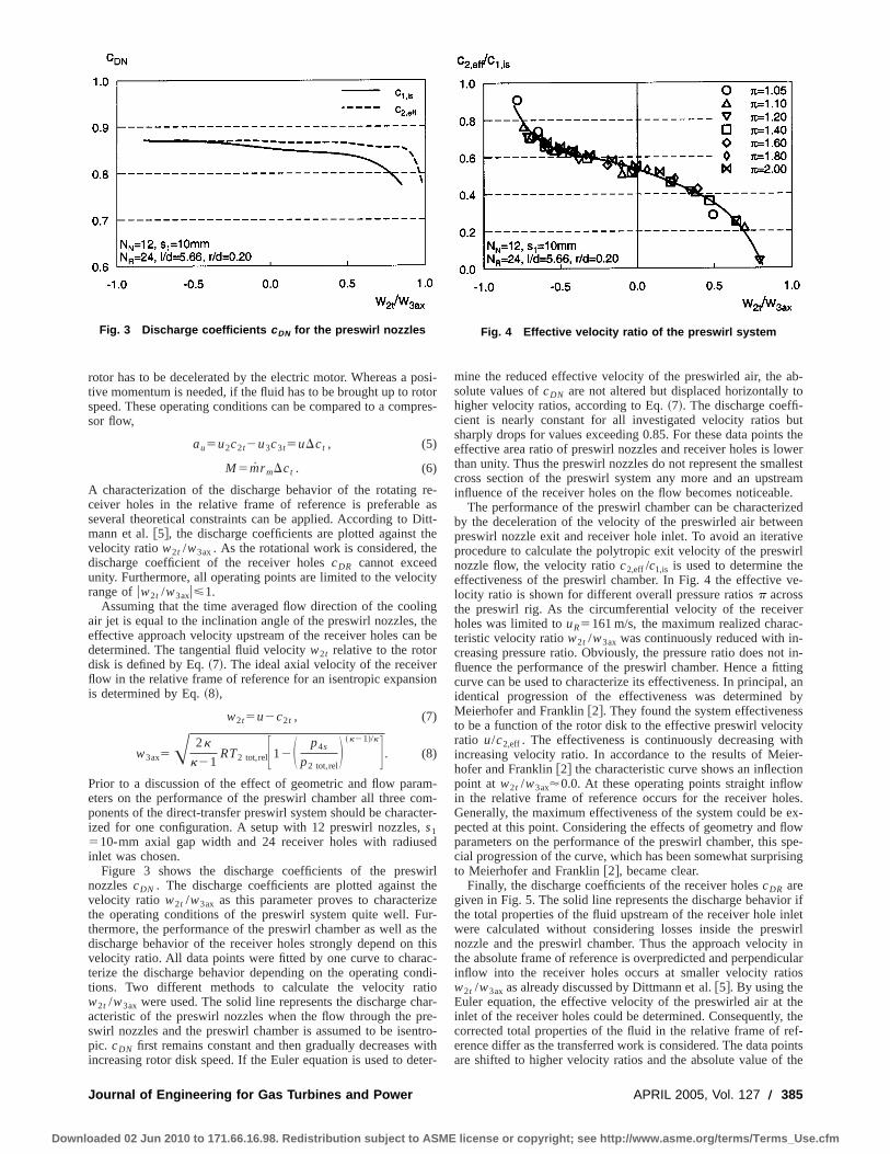
rotor has to be decelerated by the electric motor. Whereas a posi-tive momentum is needed, if the fluid has to be brought up to rotorspeed. These operating conditions can be compared to a compres-sor flow,

au5u2c2t2u3c3t5uDct , (5)

M5mr mDct . (6)

A characterization of the discharge behavior of the rotating re-ceiver holes in the relative frame of reference is preferable asseveral theoretical constraints can be applied. According to Ditt-mann et al.@5#, the discharge coefficients are plotted against thevelocity ratiow2t /w3ax. As the rotational work is considered, thedischarge coefficient of the receiver holescDR cannot exceedunity. Furthermore, all operating points are limited to the velocityrange ofuw2t /w3axu<1.

Assuming that the time averaged flow direction of the coolingair jet is equal to the inclination angle of the preswirl nozzles, theeffective approach velocity upstream of the receiver holes can bedetermined. The tangential fluid velocityw2t relative to the rotordisk is defined by Eq.~7!. The ideal axial velocity of the receiverflow in the relative frame of reference for an isentropic expansionis determined by Eq.~8!,

w2t5u2c2t , (7)

w3ax5A 2k

k21RT2 tot,relF12S p4s

p2 tot,relD ~k21!/kG . (8)

Prior to a discussion of the effect of geometric and flow param-eters on the performance of the preswirl chamber all three com-ponents of the direct-transfer preswirl system should be character-ized for one configuration. A setup with 12 preswirl nozzles,s1510-mm axial gap width and 24 receiver holes with radiusedinlet was chosen.

Figure 3 shows the discharge coefficients of the preswirlnozzlescDN . The discharge coefficients are plotted against thevelocity ratio w2t /w3ax as this parameter proves to characterizethe operating conditions of the preswirl system quite well. Fur-thermore, the performance of the preswirl chamber as well as thedischarge behavior of the receiver holes strongly depend on thisvelocity ratio. All data points were fitted by one curve to charac-terize the discharge behavior depending on the operating condi-tions. Two different methods to calculate the velocity ratiow2t /w3ax were used. The solid line represents the discharge char-acteristic of the preswirl nozzles when the flow through the pre-swirl nozzles and the preswirl chamber is assumed to be isentro-pic. cDN first remains constant and then gradually decreases withincreasing rotor disk speed. If the Euler equation is used to deter-

mine the reduced effective velocity of the preswirled air, the ab-solute values ofcDN are not altered but displaced horizontally tohigher velocity ratios, according to Eq.~7!. The discharge coeffi-cient is nearly constant for all investigated velocity ratios butsharply drops for values exceeding 0.85. For these data points theeffective area ratio of preswirl nozzles and receiver holes is lowerthan unity. Thus the preswirl nozzles do not represent the smallestcross section of the preswirl system any more and an upstreaminfluence of the receiver holes on the flow becomes noticeable.

The performance of the preswirl chamber can be characterizedby the deceleration of the velocity of the preswirled air betweenpreswirl nozzle exit and receiver hole inlet. To avoid an iterativeprocedure to calculate the polytropic exit velocity of the preswirlnozzle flow, the velocity ratioc2,eff /c1,is is used to determine theeffectiveness of the preswirl chamber. In Fig. 4 the effective ve-locity ratio is shown for different overall pressure ratiosp acrossthe preswirl rig. As the circumferential velocity of the receiverholes was limited touR5161 m/s, the maximum realized charac-teristic velocity ratiow2t /w3ax was continuously reduced with in-creasing pressure ratio. Obviously, the pressure ratio does not in-fluence the performance of the preswirl chamber. Hence a fittingcurve can be used to characterize its effectiveness. In principal, anidentical progression of the effectiveness was determined byMeierhofer and Franklin@2#. They found the system effectivenessto be a function of the rotor disk to the effective preswirl velocityratio u/c2,eff . The effectiveness is continuously decreasing withincreasing velocity ratio. In accordance to the results of Meier-hofer and Franklin@2# the characteristic curve shows an inflectionpoint at w2t /w3ax'0.0. At these operating points straight inflowin the relative frame of reference occurs for the receiver holes.Generally, the maximum effectiveness of the system could be ex-pected at this point. Considering the effects of geometry and flowparameters on the performance of the preswirl chamber, this spe-cial progression of the curve, which has been somewhat surprisingto Meierhofer and Franklin@2#, became clear.

Finally, the discharge coefficients of the receiver holescDR aregiven in Fig. 5. The solid line represents the discharge behavior ifthe total properties of the fluid upstream of the receiver hole inletwere calculated without considering losses inside the preswirlnozzle and the preswirl chamber. Thus the approach velocity inthe absolute frame of reference is overpredicted and perpendicularinflow into the receiver holes occurs at smaller velocity ratiosw2t /w3ax as already discussed by Dittmann et al.@5#. By using theEuler equation, the effective velocity of the preswirled air at theinlet of the receiver holes could be determined. Consequently, thecorrected total properties of the fluid in the relative frame of ref-erence differ as the transferred work is considered. The data pointsare shifted to higher velocity ratios and the absolute value of the

Fig. 3 Discharge coefficients c DN for the preswirl nozzles Fig. 4 Effective velocity ratio of the preswirl system



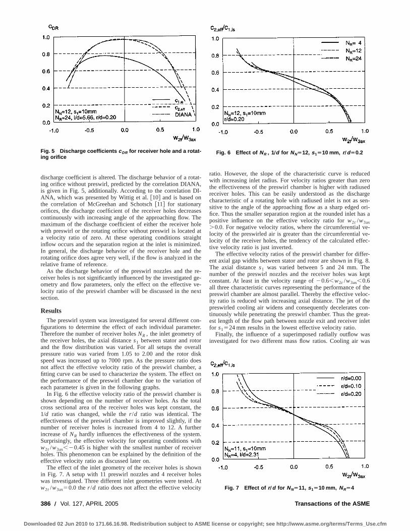
discharge coefficient is altered. The discharge behavior of a rotat-ing orifice without preswirl, predicted by the correlation DIANA,is given in Fig. 5, additionally. According to the correlation DI-ANA, which was presented by Wittig et al.@10# and is based onthe correlation of McGreehan and Schotsch@11# for stationaryorifices, the discharge coefficient of the receiver holes decreasescontinuously with increasing angle of the approaching flow. Themaximum of the discharge coefficient of either the receiver holewith preswirl or the rotating orifice without preswirl is located ata velocity ratio of zero. At these operating conditions straightinflow occurs and the separation region at the inlet is minimized.In general, the discharge behavior of the receiver hole and therotating orifice does agree very well, if the flow is analyzed in therelative frame of reference.

As the discharge behavior of the preswirl nozzles and the re-ceiver holes is not significantly influenced by the investigated ge-ometry and flow parameters, only the effect on the effective ve-locity ratio of the preswirl chamber will be discussed in the nextsection.

ResultsThe preswirl system was investigated for several different con-

figurations to determine the effect of each individual parameter.Therefore the number of receiver holesNR , the inlet geometry ofthe receiver holes, the axial distances1 between stator and rotorand the flow distribution was varied. For all setups the overallpressure ratio was varied from 1.05 to 2.00 and the rotor diskspeed was increased up to 7000 rpm. As the pressure ratio doesnot affect the effective velocity ratio of the preswirl chamber, afitting curve can be used to characterize the system. The effect onthe performance of the preswirl chamber due to the variation ofeach parameter is given in the following graphs.

In Fig. 6 the effective velocity ratio of the preswirl chamber isshown depending on the number of receiver holes. As the totalcross sectional area of the receiver holes was kept constant, the1/d ratio was changed, while ther /d ratio was identical. Theeffectiveness of the preswirl chamber is improved slightly, if thenumber of receiver holes is increased from 4 to 12. A furtherincrease ofNR hardly influences the effectiveness of the system.Surprisingly, the effective velocity for operating conditions withw2t /w3ax,20.45 is higher with the smallest number of receiverholes. This phenomenon can be explained by the definition of theeffective velocity ratio as discussed later on.

The effect of the inlet geometry of the receiver holes is shownin Fig. 7. A setup with 11 preswirl nozzles and 4 receiver holeswas investigated. Three different inlet geometries were tested. Atw2t /w3ax50.0 ther /d ratio does not affect the effective velocity

ratio. However, the slope of the characteristic curve is reducedwith increasing inlet radius. For velocity ratios greater than zerothe effectiveness of the preswirl chamber is higher with radiusedreceiver holes. This can be easily understood as the dischargecharacteristic of a rotating hole with radiused inlet is not as sen-sitive to the angle of the approaching flow as a sharp edged ori-fice. Thus the smaller separation region at the rounded inlet has apositive influence on the effective velocity ratio forw2t /w3ax.0.0. For negative velocity ratios, where the circumferential ve-locity of the preswirled air is greater than the circumferential ve-locity of the receiver holes, the tendency of the calculated effec-tive velocity ratio is just inverted.

The effective velocity ratios of the preswirl chamber for differ-ent axial gap widths between stator and rotor are shown in Fig. 8.The axial distances1 was varied between 5 and 24 mm. Thenumber of the preswirl nozzles and the receiver holes was keptconstant. At least in the velocity range of20.6,w2t /w3ax,0.6all three characteristic curves representing the performance of thepreswirl chamber are almost parallel. Thereby the effective veloc-ity ratio is reduced with increasing axial distance. The jet of thepreswirled cooling air widens and consequently decelerates con-tinuously while penetrating the preswirl chamber. Thus the great-est length of the flow path between nozzle exit and receiver inletfor s1524 mm results in the lowest effective velocity ratio.

Finally, the influence of a superimposed radially outflow wasinvestigated for two different mass flow ratios. Cooling air was

Fig. 5 Discharge coefficients c DR for receiver hole and a rotat-ing orifice

Fig. 6 Effect of NR , 1Õd for NNÄ12, s 1Ä10 mm, r ÕdÄ0.2

Fig. 7 Effect of r Õd for NNÄ11, s 1Ä10 mm, NRÄ4



fed into the rotor-stator wheelspace near the hub region. The ra-dial mass flow rate was set to 30 or 50 percent of the preswirledmainflow. The same percentage of the total mass flow rate left thepreswirl chamber through a lip seal arrangement in radial direc-tion, respectively. The effect of the superimposed radial flow onthe effective velocity ratio is depicted in Fig. 9. As shown byDittmann et al.@5# the radial outflow of coolant scarcely influ-ences the discharge behavior of the receiver holes but obviouslyhas a strong impact on the effective preswirl velocity. With in-creasing radial mass flow rate the effectiveness of the preswirledair is continuously diminished. The circumferential velocity of thefluid, which enters the preswirl chamber radially, can hardly beestimated. Both the rotational speed of the rotating lip of the innerseal and the axial through flow velocity do affect the swirl of theair exiting the inner seal. Nevertheless, the circumferential veloc-ity of the secondary flow is definitely lower than the correspond-ing velocity component of the preswirled air. Consequently, theeffective swirl of the mixed flow inside the preswirl chamber isreduced. The shift of the infection point of the characteristiccurves to positive velocity ratios may result from the few datapoints available for this configuration.

As already mentioned, the progression of the effective velocityratio was expected to be symmetric to the operation point wherestraight inflow of the receiver holes in the relative frame of refer-ence occurs. In addition, the performance of the preswirl chambershould be best for these conditions. An explanation for the con-

tinuous decrease of the effective velocity ratio can be clarified bythe total temperature ratios sketched in Fig. 10. The theoreticalcurve for an isentropic flow of the preswirl system is given by thesolid line. According to Eq.~1!, the total temperature of the cool-ing air in the relative frame of reference is equal to the totaltemperature in the absolute frame of reference foru/c2t, is50.0and 2.0. For velocity ratios smaller than 2.0, the total enthalpy ofthe cooling air is reduced in the relative frame of reference. Dueto the work done by the rotor,T2 tot,rel exceedsT2 tot for velocityratios higher than 2.0. The maximum total temperature reductionof the cooling air in the relative system is achieved atu/c2t, is51.0. The dashed line represents the total temperature ratio of thepreswirl system considering all occurring losses. The approachvelocity of the receiver holes in the absolute frame of reference islower, thus the maximum total temperature reduction in the rela-tive system is reduced. Furthermore, straight inflow to the receiverholes in the relative frame of reference occurs atu/c2t, is,1.0. Thedisplacement of this special operating point regarding the idealand the real case is indicated by the arrow. The discrepancy be-tween two corresponding data points continuously increases withincreasing velocity ratio. Thus a gradual decrease of the effectivevelocity ratio, characterizing the performance of the preswirlchamber, seems to be reasonable. The actual total temperaturereduction depends on the pressure ratio across the preswirlnozzles and the velocity ratio.

Another possibility to characterize the performance of the pre-swirl chamber would be to determine the actual total temperaturedifference between absolute and relative system based on themaximum temperature reduction, which can be achieved for anisentropic flow. For positive velocity ratiosw2t /w3ax this newlygained characteristic line will correspond to the curves presentedin Figs. 6–9. Congruence for negative velocity ratios will beachieved if the left part of the curve is mirrored across a horizon-tal line through the ordinate interception atw2t /w3ax50.0. There-with all investigated effects of geometric and flow parameters onthe effective velocity ratio characterizing the preswirl chamberbecome comprehensible.

SummaryA direct-transfer preswirl system was investigated experimen-

tally. By separating the occurring losses of the flow, all threecomponents, namely the preswirl nozzles, the preswirl chamber,and the receiver holes, could be characterized.

Discharge coefficients of the preswirl nozzlescDN were deter-mined in the absolute frame of reference, whereas the dischargecoefficients of the receiver holescDR were defined in the relativeframe of reference. Thus the work done by the rotor and the

Fig. 8 Effect of s 1 for NNÄ12, NRÄ24, r ÕdÄ0.2

Fig. 9 Effect of m rad for NNÄ12, s 1Ä10 mm, NRÄ4, r ÕdÄ0.0

Fig. 10 Cooling air total temperature in the relative frame ofreference



change of the total enthalpy of the cooling air could be taken intoaccount. The Euler equation was applied to the preswirl system toestimate the velocity of the preswirled cooling air at the inlet ofthe receiver holes. If the deceleration of the fluid is considered,the discharge behavior of the receiver holes can be compared tothe discharge characteristic of rotating orifices with parallel ap-proaching flow to the orifice axis. The discharge behavior of thereceiver holes is strongly dependant on the velocity ratiow2t /w3ax, which indicates the flow angle relative to the receiverhole axis.

Finally, the performance of the preswirl chamber was charac-terized by the effective velocity ratio of the preswirled flow. Sev-eral geometric parameters of the preswirl system were varied toinvestigate the effect on the systems effectiveness. Additionally aradial outflow was superimposed to the preswirled mainflow. Ingeneral, the effective velocity ratio does not depend on the overallpressure ratio across the preswirl system but is strongly influencedby the operating point defined by the velocity ratiow2t /w3ax.Additionally, the performance of the preswirl system can be de-fined by the total temperature ratioT2 tot,rel/T0 tot . The highestperformance is achieved at operating conditions where straightinflow of the receiver holes in the relative frame of referenceoccurs.

Based on the investigated parameters the following tendencieswere obtained. The effect of the number of receiver holes seems tobe secondary, as long asNR is equal or higher than the number ofpreswirl nozzles. In principal, the systems performance increaseswith increasing number of receiver holes. Radiusing the inlet ofthe rotating receiver holes minimizes the separation region of theflow at the inlet, especially for operating conditions where theapproaching flow in the relative frame of reference is inclined tothe orifice axis. Therefore the sensitivity of the preswirl chambereffectiveness regarding the velocity ratiow2t /w3ax is reduced withincreasingr /d. A reduction of the axial gap width between statorand rotor improves the systems efficiency. However, it should bementioned that unstable flow phenomena were ascertained byDittmann et al. @5#, predominantly occurring fors155 mm,which deteriorated the discharge behavior and the effectiveness ofthe preswirl system. The occurrence of this acoustic phenomenonis not understood yet. Superimposing a radial outflow significantlyreduces the effective velocity of the preswirled air. As the circum-ferential velocity of the fluid exiting the inner seal is remarkablylower than that of the preswirled mainflow, the systems perfor-mance is diminished continuously with increasing radial massflow rate.

AcknowledgmentsThe authors wish to thank the ‘‘Forschungsvereinigung Ver-

brennungskraftmaschinen e.V.’’ for supporting the work describedin this paper. The work was also partly funded by the EU.

Nomenclature

A 5 cross-sectional area m2

c 5 velocity in the absolute frame of reference m/scD 5 discharge coefficientcp 5 specific heat J/~kg K!d 5 diameter of receiver holes m

l 5 length of receiver holes mm 5 mass flow rate kg/sM 5 momentum on the rotor Nmn 5 rotational speed 1/minN 5 number of holesp 5 pressure N/m2

r 5 radius mr m 5 pitch radius of the receiver holes mR 5 specific gas constant J/~kg K!

Ref 5 rotational Reynolds number, Ref5vrm2 /n

s1 5 axial gap between stator and rotor mT 5 temperature Ku 5 circumferential velocity m/sw 5 velocity in the relative frame of reference m/sa 5 inclination of preswirl nozzles degk 5 isentropic exponentn 5 kinematic viscosity m2/sp 5 total pressure ratio,p5p0 tot /p4sv 5 angular velocity of rotor 1/s

Subscripts

ax 5 axialeff 5 effectiveis 5 isentropicN 5 preswirl nozzleR 5 receiver hole

rad 5 radialrel 5 relative system

s 5 statict 5 tangential

tot 5 total0–4 5 position 0–4

References@1# Scricca, J. A., and Moore, K. D., 1997, ‘‘Effects of ‘Cooled’ Cooling Air on

Pre-Swirl Nozzle Design,’’ Tech. Rep. NASA/CP-98-208527, Pratt & Whitney.@2# Meierhofer, B., and Franklin, C. J., 1981, ‘‘An Investigation of a Preswirled

Cooling Airflow to a Turbine Disc by Measuring the Air Temperature in theRotating Channels,’’ ASME Paper 81-GT-132.

@3# El-Oun, Z. B., and Owen, J. M., 1988, ‘‘Pre-Swirl Blade-Cooling Effective-ness in an Adiabatic Rotor-Stator System,’’ ASME J. Turbomach.,111, pp.522–529.

@4# Wilson, M., Pilbrow, R., and Owen, J. M., 1997, ‘‘Flow and Heat Transfer ina Pre-Swirl Rotor-Stator System,’’ ASME J. Turbomach.,119, pp. 364–373.

@5# Dittmann, M., Geis, T., Schramm, V., Kim, S., and Wittig, S., 2002, ‘‘Dis-charge Coefficients of a Preswirl System in Secondary Air Systems,’’ASME J.Turbomach.,124, pp. 119–124.

@6# Kline, S., and McClintock, F. A., 1953, ‘‘Describing Uncertainties in Single-Sample Experiments,’’ Mech. Eng.~Am. Soc. Mech. Eng.!, 75, pp. 3–8.

@7# Zimmermann, H., Kutz, J., and Fischer, R., 1998, ‘‘Air System CorrelationsPart 2: Rotating Holes and Two Phase Flow,’’ ASME Paper 98-GT-207.

@8# Popp, O., Zimmermann, H., and Kutz, J., 1998, ‘‘CFD-Analysis of CoverplateReceiver Flow,’’ ASME J. Turbomach.,120, pp. 43–49.

@9# Geis, T., Rottenkolber, G., Dittmann, M., Richter, B., Dullenkopf, K., andWittig, S., 2002, ‘‘Endoscopic PIV-Measurements in an Enclosed Rotor-StatorSystem With Pre-Swirled Cooling Air,’’11th International Symposium on Ap-plications of Laser Techniques to Fluid Mechanics, Lisbon, Portugal.

@10# Wittig, S., Kim, S., Scherer, T., Jakoby, R., and Weißert, I., 1995, ‘‘Durchflußan rotierenden Wellen- und Scheibenbohrungen und Wa¨rmeubergang an rotier-enden Wellen,’’ Forschungsvereinigung Verbrennungskraftmaschinen~FVV!,Abschlußbericht, Vorhaben Nr. 465 und 536, Heft 574.

@11# McGreehan, W. F., and Schotsch, M. J., 1988, ‘‘Flow Characteristics of LongOrifices With Rotation and Corner Radiusing,’’ ASME J. Turbomach.,110, pp.213–217.



Satoshi Gamou1

Ryohei Yokoyama

Koichi Ito

Department of Energy Systems Engineering,Osaka Prefecture University,

1-1 Gakuen-cho,Sakai, Osaka 599-8531, Japan

Parametric Study on EconomicFeasibility of MicroturbineCogeneration Systems by anOptimization ApproachEconomic feasibility of microturbine cogeneration systems is investigated by analyzingrelationships between the optimal number of microturbine units and the maximum energydemands under various conditions. For this purpose, a method to obtain the maximumenergy demand at which the optimal number changes is proposed by combining a non-linear equation problem and an optimal unit sizing problem hierarchically. Based on theproposed method, a map expressing the aforementioned relationships can be illustrated.Through numerical studies carried out on systems installed in hotels by changing theelectrical generating efficiency and the capital unit cost of the microturbine cogenerationunit as parameters, the influence of the parameters on the economic feasibility of themicroturbine cogeneration system is clarified.@DOI: 10.1115/1.1806836#

Introduction

Microturbine generator units with capacities under 100 kWhave been recently paid attention to as distributed power sources@1#. The reason for this attention lies in the expectation that themicroturbine generator units will have the advantages of low ini-tial capital cost, high electrical generating efficiency for theirsmall capacities, high reliability, low NOx emission, and so on.Moreover, microturbine generators can avoid operating at lowerpart load for a broad range of electricity demand by installingplural numbers of microturbine generators. Besides, they are ex-pected as main equipment of cogeneration systems for commer-cial and public purposes@2#. Although their total energy efficiencybecomes high, they have some disadvantages in this case. Forexample, their initial capital cost becomes expensive because ofadditional heat recovery devices, and utilization of exhaust heatfrom the microturbine generator unit with a recuperator is notefficient because of its lower temperature than large scale gasturbine generators. Therefore, it is important to investigate feasi-bility of microturbine cogeneration systems for commercial andpublic purposes from an economic viewpoint. Moreover, it is alsoimportant to investigate effects of installing plural numbers ofmicroturbine cogeneration units on their economic feasibility.

The purpose of this paper is to evaluate the aforementionedeconomic feasibility rationally for various parameters, such as acapital unit cost and an electrical generating efficiency of the mi-croturbine cogeneration unit. For this purpose, a method to obtainthe maximum energy demand at which the optimal numberchanges is proposed by combining a nonlinear equation problemand an optimal unit sizing problem hierarchically. Based on thismethod, the aforementioned feasibility is evaluated by examiningthe relationships between the optimal number and the maximumenergy demands. In the following, the configurations of microtur-bine cogeneration systems investigated here are first described.Second, the evaluation method is described. Finally, numericalparametric studies are carried out on systems installed in hotels.

System ConfigurationsFigure 1 shows a schematic diagram of a microturbine cogen-

eration system. The system has the microturbine cogeneration unit~MTU!, a single-stage absorption refrigerator~RW!, a gas-firedabsorption refrigerator~RG!, a gas-fired boiler~BG!, a radiator~RD!, and a device for purchasing and reversing electricity~EP!.In this figure, though only one unit is illustrated for each kind ofequipment, there may be several units. Solid, dot-dash, dotted, andbroken lines show flows of hot water, electricity, cold water, andnatural gas, respectively.

In the system, electricity is supplied to users by purchasingelectricity through the EP from an outside electric power companyand by operating the MTU. Electricity is also used to drive cool-ing towers and other auxiliary machinery. Moreover, electricitycan be reversed through the EP to the electric power company.Exhaust heat generated from the MTU is recovered in the form ofhot water, and it is reused for space cooling through the RW, spaceheating, and other usage in a cascade way. Surplus exhaust heat isdisposed of by the RD. Cold water for space cooling is suppliedby the RW and the RG, and hot water for space heating and otherusage is supplied by the recovered exhaust heat, the RG, and theBG.

Evaluation MethodTo evaluate the feasibility of the microturbine cogeneration sys-

tems from an economic viewpoint, we clarify the relationship be-tween the number of the microturbine cogeneration units~MTUs!and the maximum energy demands. In order to achieve this pur-pose, we consider the problem of finding the maximum energydemand at which the optimal number changes its value. Its maxi-mum energy demand is the one at which the minimum annualtotal cost, which is the sum of the annual capital cost and theannual operational cost, for the system withn MTUs is equal tothat for the system withn11 MTUs. Figure 2 shows the conceptfor the problem of finding the aforementioned maximum energydemand when the kind of the number of energy demands is one.When the kind of the number of energy demands is two, theminimum annual total cost in Fig. 2 is not a curved line but acurved surface. Then, the maximum energy demand is found as aborder curve at which two curved surfaces intersect. Similarly,when the kind of the number of energy demands is three or more,the maximum energy demand is found as a border surface or aborder hypersurface. By finding the aforementioned maximum en-





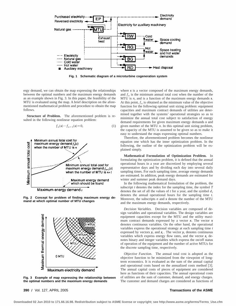
ergy demand, we can obtain the map expressing the relationshipsbetween the optimal numbers and the maximum energy demandsas an example shown in Fig. 3. In this paper, the feasibility of theMTU is evaluated using the map. A brief description on the afore-mentioned mathematical problem and procedure to obtain the mapfollows.

Structure of Problem. The aforementioned problem is re-sulted in the following nonlinear equation problem:

f n~s!2 f n11~s!50, (1)

wheres is a vector composed of the maximum energy demands,and f n is the minimum annual total cost when the number of theMTU is n, and is a function of the maximum energy demandss.At this point, f n is obtained as the minimum value of the objectivefunction for the following optimal unit sizing problem: equipmentcapacities and maximum contract demands of utilities are deter-mined together with the systems’ operational strategies so as tominimize the annual total cost subject to satisfaction of energydemand requirements for given maximum energy demandss andgiven number of the MTUn. In this optimal unit sizing problem,the capacity of the MTU is assumed to be given so as to make iteasy to understand the maps expressing optimal numbers.

Therefore, the aforementioned problem becomes the nonlinearequation one which has the inner optimization problem. In thefollowing, the outline of the optimization problem will be ex-plained simply.

Mathematical Formulation of Optimization Problem. Informulating the optimization problem, it is defined that the annualoperational hours in a year are discretized by employing severalrepresentative days and by dividing each day into several dailysampling times. For each sampling time, average energy demandsare estimated. In addition, peak energy demands are estimated forwinter and summer peak demand days.

In the following mathematical formulation of the problem, thesubscriptt denotes the index for the sampling time, the symbolTdenotes the set of all the values oft for a year, and the symboldtdenotes the annual operational hours for the sampling timet.Moreover, the subscriptsn ands denote the number of the MTUand the maximum energy demands, respectively.

Decision Variables. Decision variables are composed of de-sign variables and operational variables. The design variables areequipment capacities except for the MTU and the utility maxi-mum contract demands expressed by a vectorx. The vectorxdenotes continuous variables. On the other hand, the operationalvariables express the operational strategy at each sampling timetexpressed by vectorsyt andzt . The vectoryt denotes continuousvariables which express energy flow rates, and the vectorzt de-notes binary and integer variables which express the on/off statusof operation of the equipment and the number of active MTUs forthe discrete sampling time, respectively.

Objective Function. The annual total cost is adopted as theobjective function to be minimized from the viewpoint of long-term economics. It is evaluated as the sum of the annual capitaland operational costs based on the annualized costs method@3#.The annual capital costs of pieces of equipment are consideredhere as functions of their capacities. The annual operational costsof utilities are the sum of customer, demand, and energy charges.The customer and demand charges are considered as functions of

Fig. 1 Schematic diagram of a microturbine cogeneration system

Fig. 2 Concept for problem of finding maximum energy de-mand at which optimal number of MTU changes

Fig. 3 Example of map expressing the relationship betweenthe optimal numbers and the maximum energy demands



the maximum contract demands of utilities. The energy charge iscalculated from the system’s operational strategy. As a result, theobjective function to be minimizedJn,s i.e., the annual total cost,is defined by

Jn,s5Fn,s~xn,s!1Gn,s~xn,s!1(tPT

Vn,s,t~xn,s ,yn,s,t ,zn,s,t!dt ,

(2)

where F is the annual capital cost,G is the annual customer/demand charges, and they are functions ofx; andV is the hourlyenergy charge, and it is a function ofx, yt andzt . At this point, thevalue of f n(s) shown in Eq.~1! is the minimum value ofJn,s .

Constraints. As constraints of the optimization problem, it isnecessary to consider performance characteristics of pieces ofequipment together with hourly energy balance and supply-demand relationships of each energy flow.

The performance characteristics are formulated as relationshipsbetween input and output energy flow rates by adopting the piece-wise linear approximation@4#. For example, a part of these rela-tionships for the MTUs is expressed for each sampling time by thefollowing equations:

vMTU5pMTUuMTU1qMTUl,

uI MTUl<uMTU<uMTUl, (3)

l<n,

where p and q denote performance characteristic values, anduIandu denote lower and upper limits of input energy flow rate forone unit, respectively;l denotes an integer variable expressing thenumber of the active MTUs in a single sampling time, which is anelement of the vectorzt , andu andv are input and output energyflow rates for several units, respectively, which are elements of thevectoryt . The relationships between input and output energy flowrates for one unit of other pieces of equipment are, for example,expressed by the following equations:

v5p~x!u1q~x!d,

uI ~x!d<u<u~x!d, (4)

dP$0,1%,

whered denotes a binary variable expressing the on/off status ofoperation of equipment, which is an element of the vectorzt . InEq. ~4!, p, q, uI , and u are expressed as functions of equipmentcapacityx which is an element of the design variablesx, becausethe performance characteristics of equipment depend on theequipment capacity. At this point, let us suppose thatp(x)5p8,q(x)5q8x1q9, uI (x)5uI 8x1uI 9, and u(x)5u8x1u9. Then,p(x)u5p8u, and, consequently,p(x)u becomes a linear term. Onthe other hand,q(x)d, uI (x)d, and u(x)d include the nonlinearterm, i.e.,xd. Let xd be replaced withj, and this nonlinear termcan be linearized strictly by the following linear equations:

xI d<j< xd,(5)

x1 x~d21!<j<x,

wherexI andx denote lower and upper limits ofx. In Eq.~5!, whend50, it is derived from the upper two inequalities thatj50, andjbecomes equal toxd. Then, the lower two inequalities of Eq.~5!are inactive constraints. On the other hand, whend51, it is de-rived from the lower two inequalities thatj5x, and j becomesequal toxd as well. Then, the upper two inequalities are inactiveconstraints. As a result, Eq.~4! is rewritten by

v5p8u1q8j1q9d,

uI 8j1uI 9d<u<u8j1u9d,

xI d<j< xd, (6)

x1 x~d21!<j<x,

dP$0,1%.

On the other hand, energy balance and supply–demand rela-tionships are formulated by linear equations with energy flowratesyt at each junction for each energy flow illustrated in Fig. 1.

All these constraints are expressed simply for each samplingtime t by

Cn,s,t~xn,s ,yn,s,t ,zn,s,t!50 ~ tPT!, (7)

whereC is the vector composed of constraint functions.

Solution Method. The problem formulated and described inthe previous section is complex and of nonlinear nature because ithas the inner optimization problem. As mentioned previously, thisproblem is also one of finding the maximum energy demands asborder curves, surfaces, or hypersurfaces for the several kinds ofthe number of energy demands. Since it is very difficult to directlyfind the border curves and so on numerically, in this paper we findthe curves approximately by connecting points found as shown inFig. 4. Though Fig. 4 is an example for two kinds of the numberof energy demands, similarly we find border surfaces or hypersur-faces approximately by finding more points for several kinds ofthe number of energy demands.

The aforementioned points are found in the following way.When the kind of the number of energy demands is one and thenumber of the MTUn is given, Eq.~1! is one of finding onemaximum energy demand. Therefore, first heat-to-power ratio ofthe maximum energy demands is assumed to be constant, andunder the assumption we find the points where the optimal num-ber of the MTU changes as shown in Fig. 4. Next, we find morepoints by changing the ratio and the number, and finally we obtainthe border curves, surfaces, or hypersurfaces by connecting theobtained points.

Equation~1! of finding one maximum energy demand is solvedby Brent’s algorithm@5#, which is one combining a bisectionmethod with a secant one using not differential values but only thevalue of the functionf. The value of functionf is obtained by theoptimization problem formulated in the previous section. Theproblem results in a mixed-integer linear programming one, and itis solved by the GAMS~General Algebraic Modeling System!/CPLEX solver @6#, which is a commercial one combining thebranch and bound method with the simplex method.

Fig. 4 Concept for solution method



Numerical Study

Input Data. Cogeneration systems typically utilized in hotelsare investigated in these numerical studies. Energy demands areestimated at each of 12 discrete daily sampling times on 5 repre-sentative days in a year, i.e., winter, mid-season, summer, winterpeak demand, and summer peak demand days. As an example,

Fig. 5 shows the hourly energy demands on winter, mid-season,and summer days in the hotel with the maximum electricity de-mand of 400 kWh/h. The ratio of maximum demands of electricity: space cooling : space heating and hot water is 1:1.2:1.6. In thisnumerical study, it is assumed that the ratio of the maximum spacecooling demand to the maximum space heating and hot water onesis fixed, whereas the ratio of the maximum electricity demand tothe maximum thermal energy one is changed. By this assumption,the independent kind of the number of energy demands becomestwo, and consequently it is easy to understand results as two-dimensional illustrations as shown in Figs. 3 and 4. At this point,according to the change in the ratio of the maximum electricitydemand to the maximum thermal energy one, the demand patternshown in Fig. 5 changes linearly.

Representative values of performance characteristics and capi-tal unit costs of equipment are summarized in Table 1. These dataare based on practical systems currently used in Japan. In Table 1,the electrical generating efficiency, exhaust heat recovery effi-ciency, and capital unit cost of the microturbine cogeneration unit~MTU! are shown as parametershe, hh , anda, respectively. TheMTU investigated here is based on a unit of Capstone and itscapacity is 28 kW. The maximum output power and the electricalgenerating efficiency at the rated load of this unit are dependentgreatly on intake air temperature. Figure 6 shows the relationshipsbetween the intake air temperature and the maximum outputpower or the electrical generating efficiency at the rated load ofthis unit whenhe50.25 at 15°C. These data are based on mea-surement data and catalogs of Capstone unit. An ambient air tem-perature is adopted as the intake air temperature in these studies,and the hourly ambient air temperature on each representative dayis shown in Fig. 7. The rates for purchased/reversed electricity and

Fig. 5 Hourly energy demands „hotel with maximum electricitydemand of 400 kWh Õh…

Fig. 6 Relationship between intake air temperature and maxi-mum output power or electrical generating efficiency at ratedload

Table 1 Performance characteristics values and capital unit costs of equipment



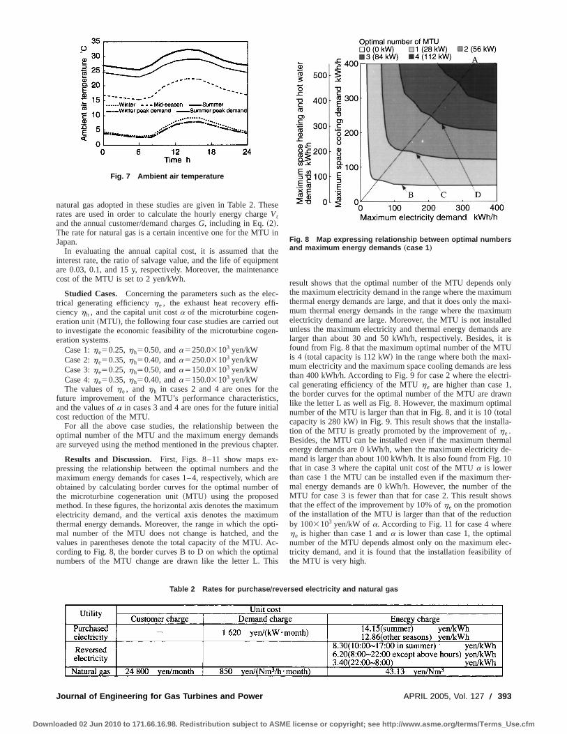
natural gas adopted in these studies are given in Table 2. Theserates are used in order to calculate the hourly energy chargeVtand the annual customer/demand chargesG, including in Eq.~2!.The rate for natural gas is a certain incentive one for the MTU inJapan.

In evaluating the annual capital cost, it is assumed that theinterest rate, the ratio of salvage value, and the life of equipmentare 0.03, 0.1, and 15 y, respectively. Moreover, the maintenancecost of the MTU is set to 2 yen/kWh.

Studied Cases. Concerning the parameters such as the elec-trical generating efficiencyhe, the exhaust heat recovery effi-ciencyhh , and the capital unit costa of the microturbine cogen-eration unit~MTU!, the following four case studies are carried outto investigate the economic feasibility of the microturbine cogen-eration systems.

Case 1:he50.25,hh50.50, anda5250.03103 yen/kWCase 2:he50.35,hh50.40, anda5250.03103 yen/kWCase 3:he50.25,hh50.50, anda5150.03103 yen/kWCase 4:he50.35,hh50.40, anda5150.03103 yen/kWThe values ofhe, and hh in cases 2 and 4 are ones for the

future improvement of the MTU’s performance characteristics,and the values ofa in cases 3 and 4 are ones for the future initialcost reduction of the MTU.

For all the above case studies, the relationship between theoptimal number of the MTU and the maximum energy demandsare surveyed using the method mentioned in the previous chapter.

Results and Discussion. First, Figs. 8–11 show maps ex-pressing the relationship between the optimal numbers and themaximum energy demands for cases 1–4, respectively, which areobtained by calculating border curves for the optimal number ofthe microturbine cogeneration unit~MTU! using the proposedmethod. In these figures, the horizontal axis denotes the maximumelectricity demand, and the vertical axis denotes the maximumthermal energy demands. Moreover, the range in which the opti-mal number of the MTU does not change is hatched, and thevalues in parentheses denote the total capacity of the MTU. Ac-cording to Fig. 8, the border curves B to D on which the optimalnumbers of the MTU change are drawn like the letter L. This

result shows that the optimal number of the MTU depends onlythe maximum electricity demand in the range where the maximumthermal energy demands are large, and that it does only the maxi-mum thermal energy demands in the range where the maximumelectricity demand are large. Moreover, the MTU is not installedunless the maximum electricity and thermal energy demands arelarger than about 30 and 50 kWh/h, respectively. Besides, it isfound from Fig. 8 that the maximum optimal number of the MTUis 4 ~total capacity is 112 kW! in the range where both the maxi-mum electricity and the maximum space cooling demands are lessthan 400 kWh/h. According to Fig. 9 for case 2 where the electri-cal generating efficiency of the MTUhe are higher than case 1,the border curves for the optimal number of the MTU are drawnlike the letter L as well as Fig. 8. However, the maximum optimalnumber of the MTU is larger than that in Fig. 8, and it is 10~totalcapacity is 280 kW! in Fig. 9. This result shows that the installa-tion of the MTU is greatly promoted by the improvement ofhe.Besides, the MTU can be installed even if the maximum thermalenergy demands are 0 kWh/h, when the maximum electricity de-mand is larger than about 100 kWh/h. It is also found from Fig. 10that in case 3 where the capital unit cost of the MTUa is lowerthan case 1 the MTU can be installed even if the maximum ther-mal energy demands are 0 kWh/h. However, the number of theMTU for case 3 is fewer than that for case 2. This result showsthat the effect of the improvement by 10% ofhe on the promotionof the installation of the MTU is larger than that of the reductionby 1003103 yen/kW of a. According to Fig. 11 for case 4 wherehe is higher than case 1 anda is lower than case 1, the optimalnumber of the MTU depends almost only on the maximum elec-tricity demand, and it is found that the installation feasibility ofthe MTU is very high.

Fig. 7 Ambient air temperature

Fig. 8 Map expressing relationship between optimal numbersand maximum energy demands „case 1 …

Table 2 Rates for purchase Õreversed electricity and natural gas



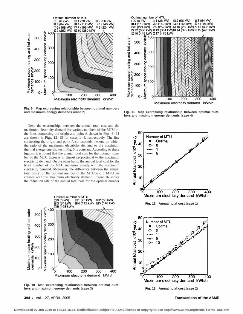
Next, the relationships between the annual total cost and themaximum electricity demand for various numbers of the MTU onthe lines connecting the origin and point A shown in Figs. 8–11are shown in Figs. 12–15 for cases 1–4, respectively. The lineconnecting the origin and point A corresponds the one on whichthe ratio of the maximum electricity demand to the maximumthermal energy one shown in Fig. 5 is constant. According to thesefigures, it is found that the annual total cost for the optimal num-ber of the MTU increase in almost proportional to the maximumelectricity demand. On the other hand, the annual total cost for thefixed number of the MTU increases greatly with the maximumelectricity demand. Moreover, the difference between the annualtotal costs for the optimal number of the MTU and 0 MTU in-creases with the maximum electricity demand. Figure 16 showsthe reduction rate of the annual total cost for the optimal number

Fig. 9 Map expressing relationship between optimal numbersand maximum energy demands „case 2 …

Fig. 10 Map expressing relationship between optimal num-bers and maximum energy demands „case 3 …

Fig. 11 Map expressing relationship between optimal num-bers and maximum energy demands „case 4 …

Fig. 12 Annual total cost „case 1 …




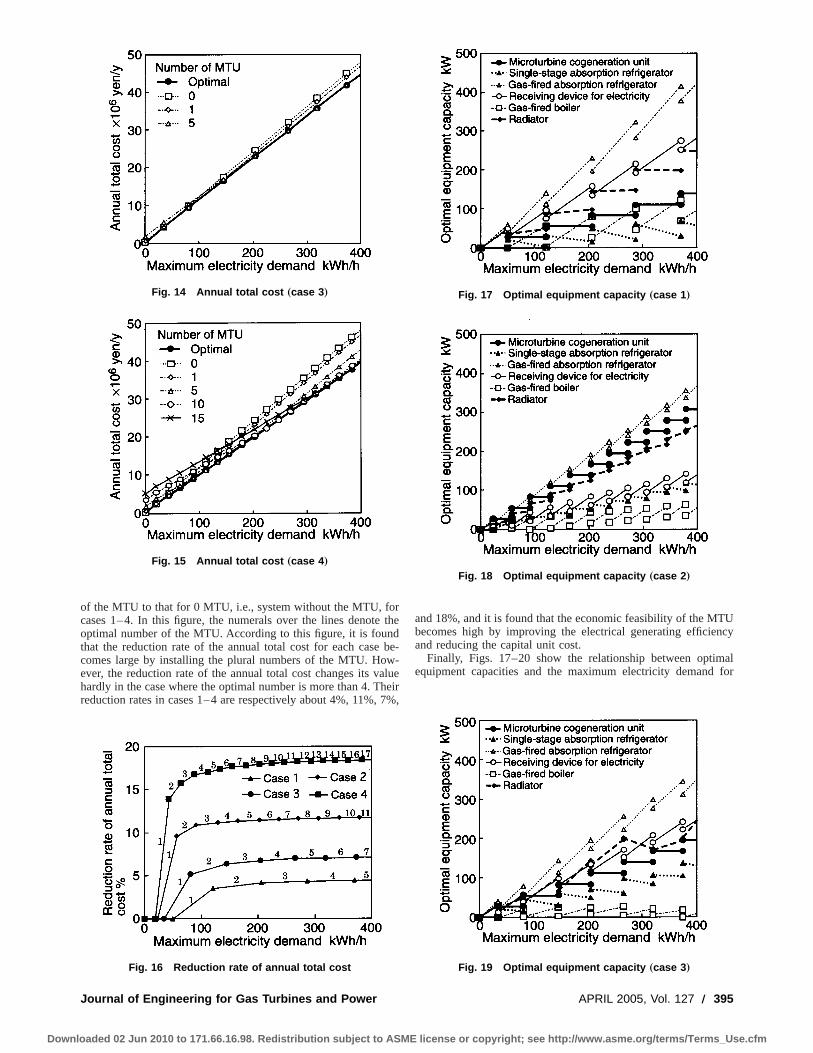
of the MTU to that for 0 MTU, i.e., system without the MTU, forcases 1–4. In this figure, the numerals over the lines denote theoptimal number of the MTU. According to this figure, it is foundthat the reduction rate of the annual total cost for each case be-comes large by installing the plural numbers of the MTU. How-ever, the reduction rate of the annual total cost changes its valuehardly in the case where the optimal number is more than 4. Theirreduction rates in cases 1–4 are respectively about 4%, 11%, 7%,

and 18%, and it is found that the economic feasibility of the MTUbecomes high by improving the electrical generating efficiencyand reducing the capital unit cost.

Finally, Figs. 17–20 show the relationship between optimalequipment capacities and the maximum electricity demand for



Fig. 16 Reduction rate of annual total cost

Fig. 17 Optimal equipment capacity „case 1 …





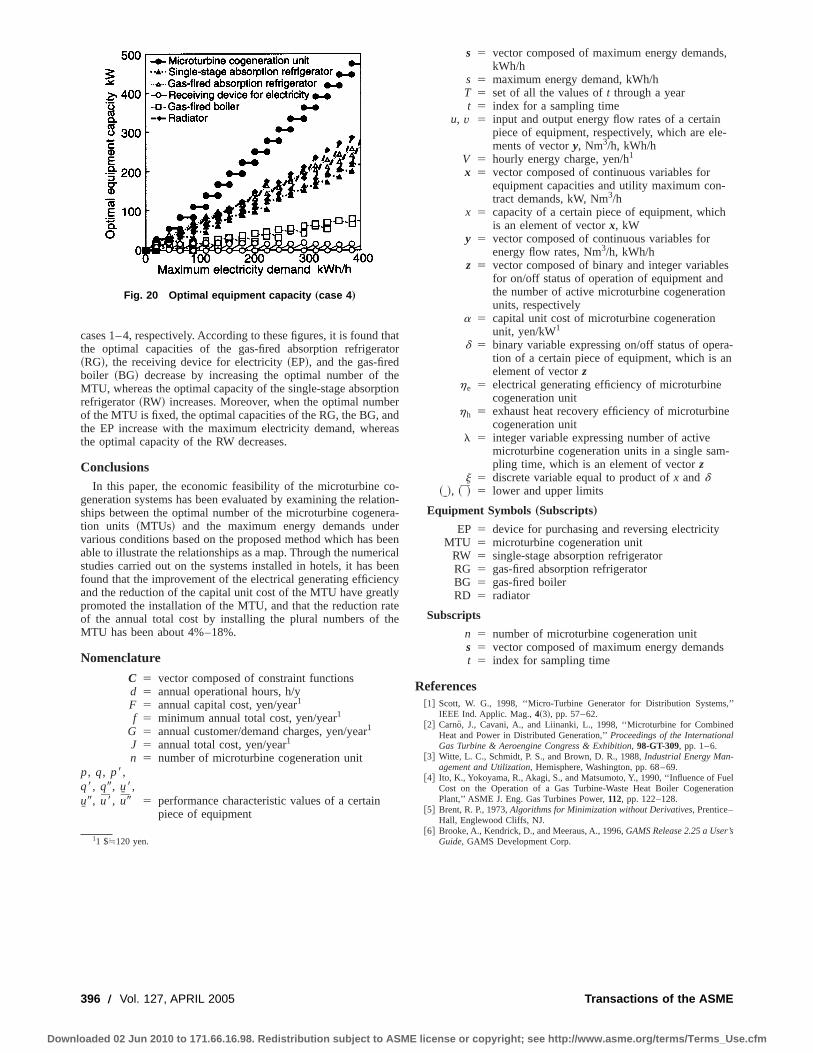
cases 1–4, respectively. According to these figures, it is found thatthe optimal capacities of the gas-fired absorption refrigerator~RG!, the receiving device for electricity~EP!, and the gas-firedboiler ~BG! decrease by increasing the optimal number of theMTU, whereas the optimal capacity of the single-stage absorptionrefrigerator~RW! increases. Moreover, when the optimal numberof the MTU is fixed, the optimal capacities of the RG, the BG, andthe EP increase with the maximum electricity demand, whereasthe optimal capacity of the RW decreases.

ConclusionsIn this paper, the economic feasibility of the microturbine co-

generation systems has been evaluated by examining the relation-ships between the optimal number of the microturbine cogenera-tion units ~MTUs! and the maximum energy demands undervarious conditions based on the proposed method which has beenable to illustrate the relationships as a map. Through the numericalstudies carried out on the systems installed in hotels, it has beenfound that the improvement of the electrical generating efficiencyand the reduction of the capital unit cost of the MTU have greatlypromoted the installation of the MTU, and that the reduction rateof the annual total cost by installing the plural numbers of theMTU has been about 4%–18%.

Nomenclature

C 5 vector composed of constraint functionsd 5 annual operational hours, h/yF 5 annual capital cost, yen/year1

f 5 minimum annual total cost, yen/year1

G 5 annual customer/demand charges, yen/year1

J 5 annual total cost, yen/year1

n 5 number of microturbine cogeneration unitp, q, p8,q8, q9, uI 8,uI 9, u8, u9 5 performance characteristic values of a certain

piece of equipment

s 5 vector composed of maximum energy demands,kWh/h

s 5 maximum energy demand, kWh/hT 5 set of all the values oft through a yeart 5 index for a sampling time

u, v 5 input and output energy flow rates of a certainpiece of equipment, respectively, which are ele-ments of vectory, Nm3/h, kWh/h

V 5 hourly energy charge, yen/h1

x 5 vector composed of continuous variables forequipment capacities and utility maximum con-tract demands, kW, Nm3/h

x 5 capacity of a certain piece of equipment, whichis an element of vectorx, kW

y 5 vector composed of continuous variables forenergy flow rates, Nm3/h, kWh/h

z 5 vector composed of binary and integer variablesfor on/off status of operation of equipment andthe number of active microturbine cogenerationunits, respectively

a 5 capital unit cost of microturbine cogenerationunit, yen/kW1

d 5 binary variable expressing on/off status of opera-tion of a certain piece of equipment, which is anelement of vectorz

he 5 electrical generating efficiency of microturbinecogeneration unit

hh 5 exhaust heat recovery efficiency of microturbinecogeneration unit

l 5 integer variable expressing number of activemicroturbine cogeneration units in a single sam-pling time, which is an element of vectorz

j 5 discrete variable equal to product ofx andd~I!, ~ ! 5 lower and upper limits

Equipment Symbols„Subscripts…

EP 5 device for purchasing and reversing electricityMTU 5 microturbine cogeneration unit

RW 5 single-stage absorption refrigeratorRG 5 gas-fired absorption refrigeratorBG 5 gas-fired boilerRD 5 radiator

Subscripts

n 5 number of microturbine cogeneration units 5 vector composed of maximum energy demandst 5 index for sampling time

References@1# Scott, W. G., 1998, ‘‘Micro-Turbine Generator for Distribution Systems,’’

IEEE Ind. Applic. Mag.,4~3!, pp. 57–62.@2# Carno, J., Cavani, A., and Liinanki, L., 1998, ‘‘Microturbine for Combined

Heat and Power in Distributed Generation,’’Proceedings of the InternationalGas Turbine & Aeroengine Congress & Exhibition, 98-GT-309, pp. 1–6.

@3# Witte, L. C., Schmidt, P. S., and Brown, D. R., 1988,Industrial Energy Man-agement and Utilization, Hemisphere, Washington, pp. 68–69.

@4# Ito, K., Yokoyama, R., Akagi, S., and Matsumoto, Y., 1990, ‘‘Influence of FuelCost on the Operation of a Gas Turbine-Waste Heat Boiler CogenerationPlant,’’ ASME J. Eng. Gas Turbines Power,112, pp. 122–128.

@5# Brent, R. P., 1973,Algorithms for Minimization without Derivatives, Prentice–Hall, Englewood Cliffs, NJ.

@6# Brooke, A., Kendrick, D., and Meeraus, A., 1996,GAMS Release 2.25 a User’sGuide, GAMS Development Corp.11 $6120 yen.




Rattan Tawney

Zahid Khan

Justin Zachary

Bechtel Power Corporation,5275 Westview Drive,Frederick, MD 21703

Economic and PerformanceEvaluation of Heat Sink Options inCombined Cycle ApplicationsThis paper is a guideline to selecting the most appropriate technology for the power plantheat sink based on water availability, site location, and wastewater disposal requirements.The paper discusses wet as well as dry cooling systems and evaluates the impact of theheat sink technology on the performance and cost of combined cycle power plants. Co-generation applications and cycling plant operations are also considered. For each pro-posed option, the performance, relative costs, and noise issues will be presented.@DOI: 10.1115/1.1839924#

Heat Sink TechnologiesIn accordance with the laws of thermodynamics, a steam cycle

rejects heat at a temperature that is much lower than the tempera-ture at which heat is added. A power plant that dissipates heat atthe lowest possible temperature will maximize cycle efficiencyand minimize the amount of heat rejected. For combined cycles,the heat dissipation scheme to the environment consists of a steamsurface condenser and/or a wet or dry cooling system. This pack-age is referred to as the heat sink. Typical heat sink technologiesin combined cycle applications include the following:

• Wet Cooling Technologies- Wet cooling tower- Once-through cooling system

• Dry Cooling Technologies- Direct dry cooling system~Air-Cooled Condenser!- Indirect dry cooling system~Heller system!

• Hybrid Cooling Technology- Wet-dry cooling system~Wet Surface Air Cooler!

Wet Cooling Tower. The heat of condensing steam is re-moved in a shell and tube heat exchanger by a continuous loopcirculating water system. The hot water is then cooled by evapo-ration in contact with air in a tower, and the heat of evaporation isdissipated into the atmosphere. Figure 1 shows a typical flowdiagram for a wet evaporative cooling tower. Theoretically, thelowest heat sink temperature achievable with a wet cooling toweris the ambient air wet bulb temperature. Because of inefficienciesin the cooling process, the cooling tower can only approach thewet bulb temperature. The closer the wet bulb is approached, thelarger and more expensive the cooling tower becomes. Apart fromthe steam condensing heat load, other auxiliary cooling loads arealso dissipated in the wet cooling tower.

Makeup water for this heat sink option is required to compen-sate for evaporation, blowdown, and drift losses from the coolingtower. Chemicals are added to the cooling tower forebay to con-trol circulating water pH, scale/corrosion, and biological growth.

Once-Through Cooling. A once-through cooling system usescold water from a nearby river, lake, or ocean and circulates itthrough the condenser to remove condensation heat and returnsthe hot water to the source. Because of the lower heat sink tem-perature relative to a wet cooling tower, once-through cooling isthe most efficient cycle heat rejection system design. Figure 2

shows a typical flow diagram for a once-through cooling system.The heat sink condensation temperature depends on the tempera-ture of the coldwater source. Specially designed intake and outfallstructures are required to direct the cooling water from the sourceto the power plant and then back to the source again. The water isfirst channeled through an intake structure where screening equip-ment prevents trash and debris from reaching the main circulatingwater pumps. Flow straightening elements designed to providestreamlined flow to the pumps are also contained in the intakestructure. The design of the intake structure must also account forchanges in the water level due to seasonal or tidal variations. Afterflowing through the condenser, the hot water is returned to theenvironment through an outfall structure designed to discharge thewater at an optimal velocity and within the thermal dischargelimit.

Direct Dry Cooling With an Air-Cooled Condenser. Drycooling systems transfer heat by convection and radiation insteadof evaporation as in wet cooling. This typically results in higherheat sink temperatures and lower cycle efficiencies relative to wettowers. This is because the heat transfer process removes latentheat from the condensing steam to the sensible heat of the ambientair. The ambient dry bulb temperature controls the condensingtemperature and pressure achievable with dry cooling. This is al-ways higher than the wet bulb temperature, which is the control-ling variable for the wet towers. In an air-cooled condenser~ACC!, the condensing heat is dissipated directly into the atmo-sphere without using an intermediate medium such as coolingwater. Figure 3 shows a typical flow diagram for an ACC. In thisarrangement, the steam exhausting the turbine is piped to the con-denser by a large diameter duct. The steam condenses in the air-cooled tube bundles. The fin tube bundles are mounted in anA-frame configuration and mounted on a steel structural support.The steam enters the tube bundles at the top of the A frame andcondenses in the tube. The heat is removed by air blown over theexterior of the tube bundle surface by a forced draft fan. Noncon-densibles are drawn off by air ejection equipment. The condensatedrains into a collection tank and is then sent back to the heatrecovery steam generator’s~HRSG’s! feedwater system.

Indirect Dry Cooling System „Heller…. The indirect drycooling system uses circulating water~steam condensed to water!to transfer the condensation heat to the air-cooled heat exchangerbundles. Cooled water from the dry cooling tower flows back to ajet condenser causing the turbine exhaust steam to condense. Thedirect contact between the circulating water and the condensingsteam results in a small condenser volume. The ambient dry bulbcontrols the heat sink temperature in this arrangement. Becausethe indirect system requires the use of two heat transfer processes~steam condenser and air-cooled heat exchangers!, the logarithmic




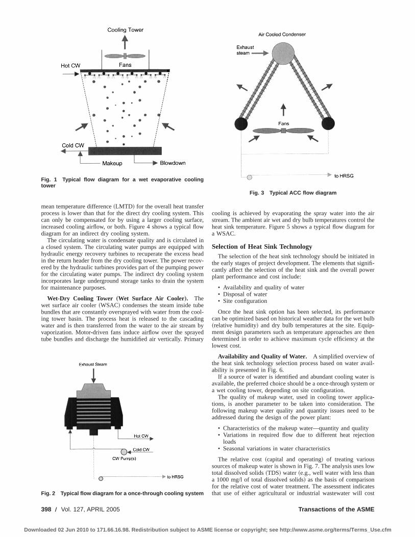
mean temperature difference~LMTD ! for the overall heat transferprocess is lower than that for the direct dry cooling system. Thiscan only be compensated for by using a larger cooling surface,increased cooling airflow, or both. Figure 4 shows a typical flowdiagram for an indirect dry cooling system.

The circulating water is condensate quality and is circulated ina closed system. The circulating water pumps are equipped withhydraulic energy recovery turbines to recuperate the excess headin the return header from the dry cooling tower. The power recov-ered by the hydraulic turbines provides part of the pumping powerfor the circulating water pumps. The indirect dry cooling systemincorporates large underground storage tanks to drain the systemfor maintenance purposes.

Wet-Dry Cooling Tower „Wet Surface Air Cooler…. Thewet surface air cooler~WSAC! condenses the steam inside tubebundles that are constantly oversprayed with water from the cool-ing tower basin. The process heat is released to the cascadingwater and is then transferred from the water to the air stream byvaporization. Motor-driven fans induce airflow over the sprayedtube bundles and discharge the humidified air vertically. Primary

cooling is achieved by evaporating the spray water into the airstream. The ambient air wet and dry bulb temperatures control theheat sink temperature. Figure 5 shows a typical flow diagram fora WSAC.

Selection of Heat Sink TechnologyThe selection of the heat sink technology should be initiated in

the early stages of project development. The elements that signifi-cantly affect the selection of the heat sink and the overall powerplant performance and cost include:

• Availability and quality of water• Disposal of water• Site configuration

Once the heat sink option has been selected, its performancecan be optimized based on historical weather data for the wet bulb~relative humidity! and dry bulb temperatures at the site. Equip-ment design parameters such as temperature approaches are thendetermined in order to achieve maximum cycle efficiency at thelowest cost.

Availability and Quality of Water. A simplified overview ofthe heat sink technology selection process based on water avail-ability is presented in Fig. 6.

If a source of water is identified and abundant cooling water isavailable, the preferred choice should be a once-through system ora wet cooling tower, depending on site configuration.

The quality of makeup water, used in cooling tower applica-tions, is another parameter to be taken into consideration. Thefollowing makeup water quality and quantity issues need to beaddressed during the design of the power plant:

• Characteristics of the makeup water—quantity and quality• Variations in required flow due to different heat rejection

loads• Seasonal variations in water characteristics

The relative cost~capital and operating! of treating varioussources of makeup water is shown in Fig. 7. The analysis uses lowtotal dissolved solids~TDS! water~e.g., well water with less thana 1000 mg/l of total dissolved solids! as the basis of comparisonfor the relative cost of water treatment. The assessment indicatesthat use of either agricultural or industrial wastewater will cost

Fig. 1 Typical flow diagram for a wet evaporative coolingtower

Fig. 2 Typical flow diagram for a once-through cooling system

Fig. 3 Typical ACC flow diagram



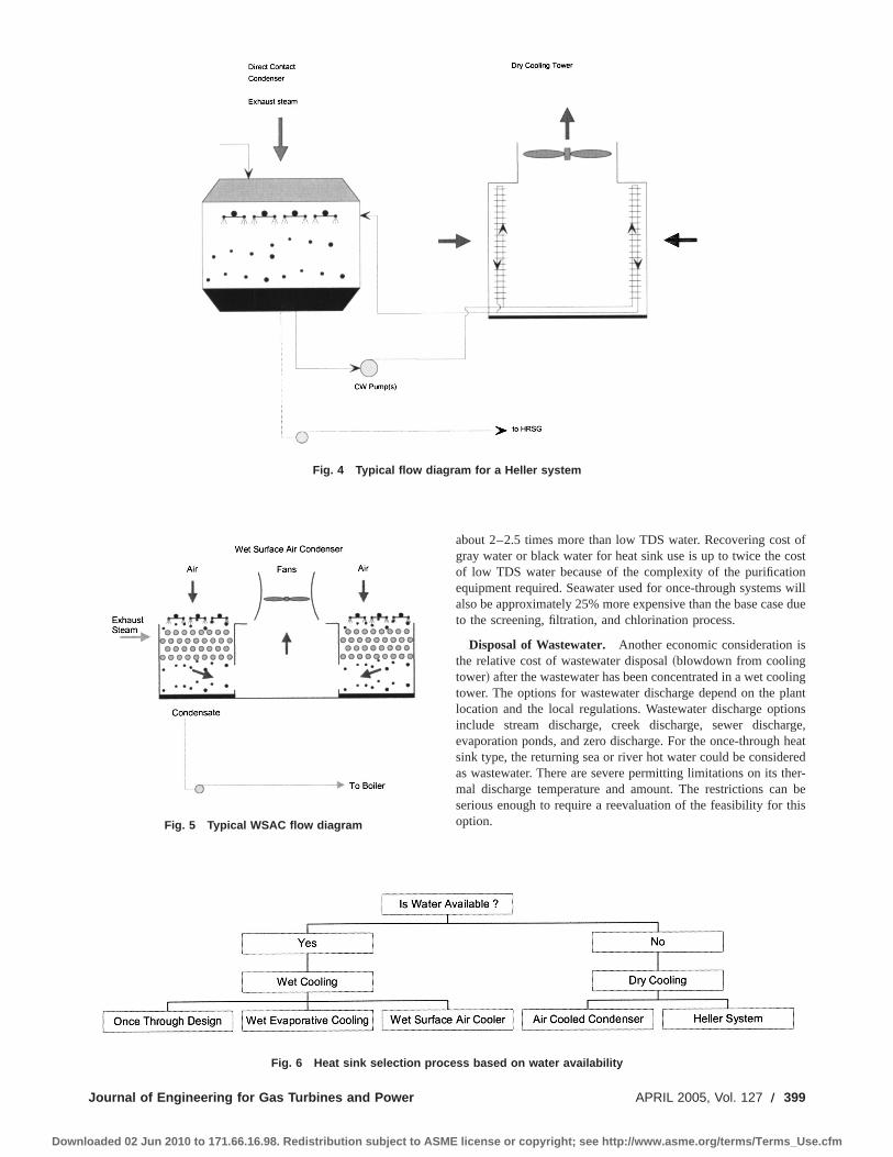
about 2–2.5 times more than low TDS water. Recovering cost ofgray water or black water for heat sink use is up to twice the costof low TDS water because of the complexity of the purificationequipment required. Seawater used for once-through systems willalso be approximately 25% more expensive than the base case dueto the screening, filtration, and chlorination process.

Disposal of Wastewater. Another economic consideration isthe relative cost of wastewater disposal~blowdown from coolingtower! after the wastewater has been concentrated in a wet coolingtower. The options for wastewater discharge depend on the plantlocation and the local regulations. Wastewater discharge optionsinclude stream discharge, creek discharge, sewer discharge,evaporation ponds, and zero discharge. For the once-through heatsink type, the returning sea or river hot water could be consideredas wastewater. There are severe permitting limitations on its ther-mal discharge temperature and amount. The restrictions can beserious enough to require a reevaluation of the feasibility for thisoption.

Fig. 4 Typical flow diagram for a Heller system

Fig. 5 Typical WSAC flow diagram

Fig. 6 Heat sink selection process based on water availability



The results of a cost analysis conducted to assess the relativecost ~capital and operating! of wastewater disposal are summa-rized in Fig. 8. The analysis uses the cooling pond as the basis ofcomparison for the relative cost of water treatment.

From the analysis, the ‘‘zero discharge’’ option is the most ex-pensive and could cost as much as four times more than the cool-ing pond option. Therefore, the zero discharge option should beused only where stringent environmental laws require it. Success-

Fig. 7 Cost of makeup water sources for heat sink options relative to low TDS water

Fig. 8 Cost of wastewater disposal for heat sink options relative to an impoundment system



ful removal of contaminated water for zero discharge conditionsinvolves very complex hardware and systems integration pro-cesses. Other disposal alternatives, such as discharge to watertreatment plants, are at least twice the basic cost due to associatedcost of the water treatment.

Site Configuration. Each heat sink option has specific layoutrequirements. For mechanical draft wet cooling towers, spacingand orientation affect thermal performance due to re-circulationand wind direction. Rectangular cooling towers are oriented par-allel to the prevailing wind so that the exit air is blown away fromthe inlet.

Once-through cooling systems must be located near a largenatural body of water. If the source for the body of water is notnearby, the necessary extended lengths of circulating water pipingand larger pumps will increase the equipment cost as well asparasitic pumping power. Under such conditions, a detailed evalu-ation should be conducted to confirm the viability of this option.

Direct and indirect dry cooling systems require a large amountof space. Their location within the site perimeter should avoidrestrictions to the inlet airflow.

Air-cooled condensers should be located close to the turbinebuilding to minimize the pressure drop between the steam turbineand the condenser, reducing steam duct cost and improving cycleefficiency. In general, ACCs require a large, symmetrical plotspace to accommodate their rectangular shape. Any irregular lot orunusual site requires creative and unconventional solutions.

Cycling and Cogeneration Considerations

Cycling Considerations. The merchant plant concept impliesthat electric power must be supplied to the grid only when it iscommercially justifiable. Such requirements must typically be meton very short notice. Therefore, these plants need to be started upquickly and should have flexible operating ranges. Merchantplants are normally in cycling service, which can be consideredpart-load operation or daily on/off operation. Heat sink consider-ations for a cycling plant require special features as describedbelow:

• Use an auxiliary boiler to sparge the condenser hotwell toprevent the condensate from subcooling

• Maintain condenser vacuum during periods of shutdown• Use a cooling tower bypass to shut-off cells for low load

operation• Use pre-coat condensate treatment~condensate polisher! with

ACC, which may have large surface areas of carbon steel incontact with steam and condensate

• Include provisions to control all heat sink fans from the con-trol room

Cogeneration Applications. Cogeneration is the simulta-neous production of electrical and thermal energy. Cogenerationplants must also consider the quality and quantity of water re-turned to the power plant from the process. Depending on thequality of the returned water, further deaeration and chemicaltreatment may be necessary. If all the exported water is not re-turned, additional cycle makeup will be required. An external de-aerator will be required if the total cycle makeup exceeds 3%–5%.

Comparative Analysis

Comparative Analysis of Heat Sink Technologies. To as-sess the impact of different heat sink options, a combined cycleplant computer model was developed using a standard, commer-cially available simulation package~Thermoflow, Inc. software!.The base case for this comparison of different heat sink technolo-gies is the wet cooling tower. In our modeling, the plant configu-ration and ambient conditions were maintained identical for allcases. The only variations allowed were due to the changes in theheat sink design parameters. The selected configuration includes

two gas turbines, two HRSGs, and one steam turbine~23231!.No steam extraction from the cycle was considered. No restric-tions on either the water availability or the site configuration wasconsidered in the model. In calculating net power output and heatrate, the specific auxiliary loads associated with each type of heatsink option were subtracted. Plant thermal performance wasevaluated by the different condensing pressures resulting fromeach particular heat sink technology. A higher backpressure resultsin a lower power output and worse heat rate. The heat dissipationcapability of each of the technologies is dependent on ambientconditions. The thermal performance is dependent on the wet bulbtemperature for the wet cooling tower and is related to dry bulbtemperature for the ACC and indirect dry cooling tower. For theonce-through condenser using river or seawater, the heat sink tem-perature for the process is the river or seawater temperature. Toproduce meaningful results for the comparison, design parametersfor condensing and/or heat dissipation equipment sizing, such asapproach temperatures, rise, and other applicable criteria, arebased on industry trends. The results of the analysis for the ther-mal performance and associated cost on a comparative basis areillustrated in the bar chart format.

Condenser Pressure. Figure 9 presents the expected back-pressures for each heat sink option. The results are relative, basedon the wet cooling tower backpressure equal to 1. A WSAC willhave the same backpressure as the wet cooling tower at the sameambient wet bulb temperature. Under these conditions, a plantsubstituting an ACC or a indirect dry cooling tower for a wettower will have a backpressure that is approximately 2.1 timeshigher, because the ACC and indirect dry cooling towers are gov-erned by the dry bulb temperature. In contrast, a once-throughcondenser will have a backpressure that is about 40% lower thanthe base case.

Electrical Power Output. The electrical power output com-parison in Fig. 10 shows that the net output is higher at lower heatsink temperatures with corresponding backpressures. The com-parison indicates that ‘‘dry options,’’ such as ACC and indirect drycooling systems, are about 4%–5% lower in power output com-pared with a wet cooling tower. Direct use of cooling water asshown in the once-through condenser could yield approximately2% more power output.

Heat Rate. The impact on the net plant heat rate is shown inFig. 11. A once-through condenser option will have about 2%better heat rate than the wet cooling tower. For this option itshould be emphasized that, in addition to lower condensing pres-sure and temperature, the auxiliary loads are relatively smaller.The net plant heat rate of dry tower options such as ACC andindirect dry cooling systems can be about 5% worse than that ofthe wet cooling tower.

Fig. 9 Condenser pressure comparison relative to a wet cool-ing tower



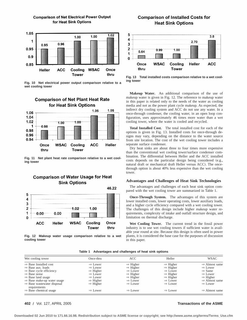
Makeup Water. An additional comparison of the use ofmakeup water is given in Fig. 12. The reference to makeup waterin this paper is related only to the needs of the water as coolingmedia and not as the power plant cycle makeup. As expected, theindirect dry cooling system and ACC do not use any water. In aonce-through condenser, the cooling water, in an open loop con-figuration, uses approximately 46 times more water than a wetcooling tower, where the water is cooled and recycled.

Total Installed Cost. The total installed cost for each of theoptions is given in Fig. 13. Installed costs for once-through de-signs may vary, depending on the distance to the water sourcefrom site location. The cost of the wet cooling tower includes aseparate surface condenser.

Dry heat sinks are about three to four times more expensivethan the conventional wet cooling tower/surface condenser com-bination. The differential between Heller and the ACC installedcosts depends on the particular design being considered~e.g.,natural draft or mechanical draft Heller versus ACC!. The once-through option is about 40% less expensive than the wet coolingtower.

Advantages and Challenges of Heat Sink TechnologiesThe advantages and challenges of each heat sink option com-

pared with the wet cooling tower are summarized in Table 1.

Once-Through System. The advantages of this system arelower installed costs, lower operating costs, lower auxiliary loads,and a higher cycle efficiency compared with a wet cooling tower.The challenges of this design include higher makeup water re-quirements, complexity of intake and outfall structure design, andlimitation on thermal discharge.

Wet Cooling Tower. The current trend in the fossil powerindustry is to use wet cooling towers if sufficient water is avail-able year round at site. Because this design is often used in powerplants, it is considered the base case for the purposes of discussionin this paper.

Fig. 10 Net electrical power output comparison relative to awet cooling tower

Fig. 11 Net plant heat rate comparison relative to a wet cool-ing tower

Fig. 12 Makeup water usage comparison relative to a wetcooling tower

Fig. 13 Total installed costs comparison relative to a wet cool-ing tower

Table 1 Advantages and challenges of heat sink options

Wet cooling tower Once-thru ACC Heller WSAC

⇒ Base Installed cost ⇒ Lower ⇒ Higher ⇒ Higher ⇒ Almost same⇒ Base aux. loads ⇒ Lower ⇒ Higher ⇒ Higher ⇒ Lower⇒ Base cycle efficiency ⇒ Higher ⇒ Lower ⇒ Lower ⇒ Same⇒ Base noise ⇒ Lower ⇒ Higher ⇒ Higher ⇒ Lower⇒ Base land usage ⇒ Lower ⇒ Higher ⇒ Higher ⇒ Higher⇒ Base make-up water usage ⇒ Higher ⇒ Lower ⇒ Lower ⇒ Almost same⇒ Base wastewater disposal

requirements⇒ Higher ⇒ Lower ⇒ Lower ⇒ Lower

⇒ Base chemical usage ⇒ Lower ⇒ Lower ⇒ Lower ⇒ Almost same



The advantages of this system are moderate installed and oper-ating costs, auxiliary loads with moderate makeup water require-ments, and relatively good cycle efficiency. The challenges of thisdesign include cooling tower blowdown disposal, plume forma-tion at colder ambient temperatures, and disposal of any wastes~such as sludges! which may result from treatment of the makeupwater.

For wet cooling towers, plume formation and blowdown dis-posal are major concerns. To solve the plume problem, the wetcooling tower manufacturers have developed systems to abate itsformation. However, below certain ambient temperatures, theabatement process becomes ineffective and the plume reappearsand gradually increases in size.

Dry Cooling With Air-Cooled Condenser. The advantagesof this system are that water usage requirements are minimal andthat no issues are associated with blowdown disposal and plumeformation. The challenges of this design are higher installed costs,relatively higher noise emissions, larger footprint, and lower cycleefficiency than the base case~wet cooling tower!.

Indirect Dry Cooling System. The advantages of this systemare lower auxiliary loads and lower noise for natural draft-typeHeller systems, minimal water usage requirements, and absence ofissues associated with blowdown disposal and plume formation.The challenges of this design are higher installed costs, relativelylarger footprint, and lower cycle efficiency. An increased quantityof oxygen scavenger is also required because the jet condenserachieves an oxygen level of only 15–20 ppb in the condensate,which is higher than the typical values seen in a deaerating con-denser. The challenges of a mechanical draft-type Heller systemincludes higher auxiliary loads and higher noise.

Wet Surface Air Cooler. The advantages of this system arelower auxiliary loads, low noise, and slightly lower water usagerequirements. The wet surface air cooler has a direct temperatureapproach to the wet bulb. This provides more efficient coolingthan an ACC, which has an approach to the dry bulb temperature.At this time, this technology is not widely accepted in power plantapplications.

ConclusionThe heat sink option is often governed by factors such as site

configuration, availability of water, and water disposal. The heatsink option selection process should be initiated in the early stagesof project development to take these factors into account.

The plant performance in terms of power output and efficiencyis best for the once-through option and worst for the indirect drycooling system. The installed cost is highest for the ACC, closelyfollowed by the indirect dry cooling system unit and lowest forthe once-through system. The highest amount of make-up waterwill be consumed by the once-through option, while the indirectdry cooling system will consume the least. The probability ofplume formation is greatest for the wet cooling tower option,

whereas it is almost zero for the dry cooling systems such as ACCand Heller. The noise level is highest for the ACC, while it isalmost zero for the once-through system. The wet cooling towerwill generate the most wastewater for disposal, while dry systemssuch as ACC and indirect dry cooling will produce almost zerowastewater for disposal. The amount of real estate space needed isgreatest for the indirect dry cooling option and least for the once-through system.

The relative cost of make-up water and the cost of wastewaterdisposal are also important considerations in the selection of heatsink options. The plants using black water or industrial wastewa-ter have much higher costs. An expensive alternative for waste-water disposal will be zero discharge, with a disposal cost possi-bly four times that of a cooling pond.

The selection of a heat sink option is often site specific and isbased on variables that include water availability, site configura-tion, water disposal, ambient conditions, level of target poweroutput, anticipated hours of operation, Power Purchase Agreementstructure, and Owner’s economic evaluation factors for plant out-put, heat rate, and operations and maintenance costs.

While it is difficult to make any specific recommendations, thefollowing conclusions would be valid for a majority of situations:

• For sites with scarce water resources, dry cooling systemssuch as the ACC and indirect dry cooling options will mostlikely be the preferred choice.

• For regions with adequate water availability and provisionsfor water disposal, wet cooling systems such wet coolingtower and WSAC will most likely be the preferred choice.

• For sites with a nearby river, ocean, lake, etc., once-throughand/or wet cooling tower will be the option of choice.

• For regions near residential areas where noise is an issue,ACC may not be preferred.

• For peaking applications where electricity can be sold at ahigh price, once-through or wet cooling tower may offer areasonable solution.

• For sites with limited water availability, parallel condensingsystems consisting of an ACC and a wet cooling tower maybe considered.

AcknowledgmentsThanks to Sam Keith and Dave Ugolini, from Bechtel, for their

valuable contributions and comments regarding this paper.

Nomenclature

ACC 5 air cooled condenserCW 5 circulating water

LMTD 5 logarithmic mean temperature differenceTDS 5 total dissolved solids

WSAC 5 wet surface air coolerHRSG 5 heat recovery steam generator



Francisco Sancho-Bastos

Horacio Perez-Blanco

Department of Mechanical and NuclearEngineering,

The Pennsylvania State University,137 Reber Building,

University Park, PA 16802-1412

Cogeneration System Simulationand Control to Meet SimultaneousPower, Heating, and CoolingDemandsGas turbines are projected to meet increasing power demand throughout the world. Co-generation plants hold the promise of increased efficiency at acceptable cost. In a generalcase, a cogen plant could be able to meet power, heating and cooling demands. Yet thosedemands are normally uncoupled. Control and storage strategies need to be explored toensure that each independent demand will be met continuously. A dynamic model of amid-capacity system is developed, including gas and steam turbines, two heat recoverysteam generators (HRSG) and an absorption-cooling machine. Controllers are designedusing linear quadratic regulators (LQR) to control two turbines and a HRSG with somenovelty. It is found that the power required could be generated exclusively with exhaustgases, without a duct burner in the high-pressure HRSG. The strategy calls for fuel andsteam flow rate modulation for each turbine. The stability of the controlled system and itsperformance are studied and simulations for different demand cases are performed.@DOI: 10.1115/1.1789993#

IntroductionIn the present work we address how a cogeneration system can

be controlled to satisfy transient power, heating and cooling de-mands, which are essentially independent of each other. The in-creasingly used@1# Brayton cycle discharges waste heat of con-siderable exergetic value. Hence, cogeneration schemes@2–7#have been studied, leading to the combination of Brayton andRankine cycles@8#, where the waste heat from the Brayton cycledrives the Rankine cycle. In some applications, some of the wasteheat is used to cool the inlet air for the gas turbine, resulting inincreased power output, but not in increased generating efficiency@6#.

In cogen systems the products of combustion are used at hightemperature by one component or cycle, and reject heat is used atprogressively lower temperatures by other components. Eachcomponent in the energy cascading chain must be working atdesign. The transient nature of utility demand negates, in mostcases, the possibility that all subsystems will work constantly attheir design capacity. Clearly, the goal should be to fully use everyunit of fuel to satisfy demand, but this may not always be pos-sible, even if storage of some type of energy is adopted@4#. Somefuel use as backup may be called for. The issue of controllingthermal systems comprising multiple components has been ad-dressed in the literature@2,3,7#. Generally, it was concluded thatpower-generating systems can respond to faults effectively, andthat also they can follow loads within specified limits.

The system considered here provides power, heat, and cooling~Fig. 1! and it is somewhat more complex than previously studiedpower-generating facilities. A gas turbine supplies power to a userand the exhaust gas produces high-pressure steam to run a steamturbine. Low-pressure steam serves a thermal demand and, via anabsorption machine, a cooling demand. As far as power genera-tion goes, the system under consideration is not unlike a medium-capacity cogeneration system that could be installed in an indus-

trial concern or small city. The low-pressure HRSG with twoindependent users is not commonly found, and to ascertain itsfeasibility and control is part of the thrust of this work.

In what follows, we describe the models and controls adoptedfor each component and how each element was integrated into asystem. We also explain how we selected different loads, attempt-ing to reflect demand profiles commonly found. We completesimulations at different ambient temperatures and with differentparameters. The ability of each subsystem to respond to changesin loads or to store energy is studied.

Plant ModelsIn the system schematic~Fig. 1!, we describe each stream with

a number. In the gas turbine, the power production rate~1! isdetermined by the mass flow rate of natural gas~2! and the posi-tion of the Inlet Guide Vanes~IGVs!. Controlled variables are therotational speed~3! and the exhaust gas temperature~5!. Theformer two determine the amount and rate of potential heat recov-ery. The exhaust gas stream~5! flows to HRSG I, where the su-perheated steam stream~6! necessary to activate the steam turbineis produced. The steam turbine produces power~7!, and the low-pressure exit steam~8! flows to the condenser. After condensation,the water is returned to HRSG I. The combined power productionfrom both turbines meets the total electric power demand.

The exhaust gas from HRSG I~9!, flows to the low-pressureHRSG II. A design capacity of 16 kg/s of steam was adopted forthe former, whereas lower capacity of 4 kg/s was adopted for thelatter. The capacities depend on the selected steam pressure levelsand could change responding to design optimization, not at-tempted here. The steam generated by HRSG II is used to coverthe steam requirements of the absorption-cooling machine and ofa process heat consumer. The cooling machine provides air con-ditioning to a load with a time profile akin to those of officebuildings, whereas the steam demand varies stepwise in time.Hence, various intermittent process heating operations, such asdrying or water heating, are simulated.

A burner is added to the second HRSG for those instances whenthe exhaust gas mass flow rate is not large enough to meet the

Contributed by the International Gas Turbine Institute~IGTI! of THE AMERICANSOCIETY OF MECHANICAL ENGINEERSfor publication in the ASME JOURNAL OFENGINEERING FOR GAS TURBINES AND POWER. Paper presented at the Interna-tional Gas Turbine and Aeroengine Congress and Exhibition, Atlanta, GA, June16–19, 2003, Paper No. 2003-GT-38840. Manuscript received by IGTI, Oct. 2002;final revision, Mar. 2003. Associate Editor: H. R. Simmons.



requirements of the HRSG. Each component is modeled and con-trolled separately. The models are invalid for startup or shutdowntransients.

Gas Turbine. The gas turbine model is based on the work ofCamporeale@9,10#. In general, the ratio of the Laplace transformof the output to the Laplace transform of the input of a plantdepends on the parameters of the plant and on the value of thetransform variables. Since the gas turbine model has two inputs,namely, fuel mass flow rate and IGV position, and two outputs,namely, angular velocity and exhaust temperature, either input caninfluence either output. The two inputs and two outputs in the gasturbine model will have four transfer functions that are presentedin a 232 transfer matrix~Eq. ~1!! @11–13#.

F~s!5S ÃGT~s!

mf~s!

ÃGT~s!

r IGV~s!

TGT~s!

mf~s!

TGT~s!

r IGV~s!D (1)

The transfer functions in thes plane readily yield insights intogas turbine stability and response to simple inputs. Yet, the modelpresents multiple outputs and multiple inputs, which are betterhandled for optimization purposes in the state-space representa-tion. Hence, the model of Eq.~1! was translated into state space.

Minor changes were made to the original model proposed byCamporeale@14#, allowing larger air and fuel mass flow rates,adjusted to meet the efficiency and rotational inertia of the se-lected turbine. An additional feature in the present model allowssimulation of the effect of ambient temperature on power produc-tion.

Steam Turbine. The steam turbine model is a simplified ver-sion of the gas turbine one. In the steam turbine, the angularvelocity is of importance, but the exhaust temperature is not.Then, the exhaust temperature state was eliminated from the tur-bine model, resulting in a SISO system@15#, where the only inputis the power generated, and the only output is the rotational speed.The mass of steam is considered a disturbance~in a control sense!introduced by the HRSG I in order to maintain its steam tempera-ture and pressure at the set point as it will be explained later on.Model parameters were adjusted to obtain a realistic time re-sponse to a step input.

HRSG I and II. Detailed HRSG simulation is difficult, forthe attending heat transfer equations are nonlinear. In addition,each pressure level within the HRSG requires an economizer tubebundle for preheating the condensate, an evaporator bundle, and asuperheater bundle to ensure dry steam output. Each section of theHRSG is connected to the same drum, and there is a drum foreach pressure level. The difficulty of modeling a HRSG lies on the

counter flow nature of the arrangement, and the complexity ensu-ing from the arrangement required the simplifying assumptionsbelow.

Applying the First Law of Thermodynamics and assumingoverall constant vapor quality in the HRSG we get@14#

Q5MHRSGdTH

dt1ms,e~he2u1,sat!1ms,i~u1,sat2hi ! (2)

The rate of heat transfer from the gas to the steam is a functionof the heat transfer coefficients for each HRSG section, and of thetemperature difference for each section. Modeling this complexsituation has proven difficult in some studies, even at steady state@6,16#, and consequently, a simplification was sought. It was rea-soned that when steady-state conditions apply, the evaporatorpinch ~i.e., the temperature difference between the gas and thesteam at the evaporator section gas exit! determines the amount ofsteam produced. If this pinch increases, heat transfer rates willincrease for the three sections of the HRSG, and the converse willoccur if it decreases. Hence, the HRSG capacity was simply madea function of the pinch, namely,

Q5UA~Tgp2Tevap! (3)

whereTgp is the vaporization temperature of the steam, which isthe variable to be controlled in order to maintain the steady-statepressure. The gas temperature at the pinch is calculated by thefollowing equation, which represents the HRSG energy balance:

Tgp5ms,e~he2h1,sat!

mgcpg1Tgi (4)

In forced convection applications, the convective heat transfercoefficient is proportional to the 0.8 power of the flow rate, if theflow is turbulent. Assuming this to be the case, and factoring inthe fact that the gas side tends to control the heat transfer rate, weobtain finally,

Q5kmg0.8S ms,e~he2h1,sat!

mgcpg1Tgi2TevapD (5)

Rearranging terms we arrive at

Q5kmg

0.8ms,e~he2h1,sat!

mgcpg1kmg

0.8Tgi1kmg0.8Tevap (6)

Combining Eqs.~2!, ~5!, and~6! yields,

MHRSGdTevap

dt1ms,e~he2u1,s!1ms,i~u1,s2hi !

5kmg

0.8ms,e~he2h1,sat!

mgcpg1k•mg

0.8Tgi2 kmg0.8Tevap (7)

The simplification embodied in Eq.~3! results in a SISO systemwhere the only state is the steam evaporation temperature for eachHRSG I and II. For HRSG I the only input is the mass of steamreleased to the steam turbine, and it presents two different distur-bances that are the mass flow of gas from the gas turbine and itstemperature. The rest of the coefficients were assumed to be con-stants, namely, their calculated values at design conditions wereadopted. For HRSG II the input is the mass flow rate of exhaustgas, and the mass of steam delivered to users and chiller and theexhaust gas temperature are considered control disturbances.

In order to be able to apply linear control theory, it is necessaryto linearize Eq.~7! about the design values for both HRSGs. Thelinearization yields two first-order differential equations for eachHRSG of the form,

MHRSG•cHRSG

dTevap

dt1K1Tevap5K2ms,e (8)

Fig. 1 Cogeneration plant diagram



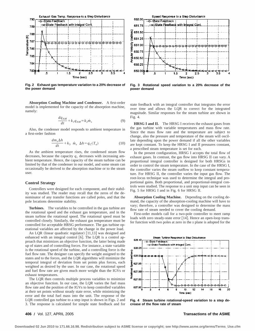
Absorption Cooling Machine and Condenser. A first-ordermodel is implemented for the capacity of the absorption machine,namely:

dqAM

dt1k1qAM5k2ms (9)

Also, the condenser model responds to ambient temperature ina first-order fashion

dmsDh

dt1k3 ms Dh5qC~Ta! (10)

As the ambient temperature rises, the condensed steam flowdecreases, because the capacityqc decreases with increasing am-bient temperature. Hence, the capacity of the steam turbine can belimited by that of the condenser in our model, and some steam canoccasionally be derived to the absorption machine or to the steamuser.

Control StrategyControllers were designed for each component, and their stabil-

ity was studied. The reader may recall that the zeros of the de-nominator of any transfer functions are called poles, and that thepole locations determine stability.

Turbines. The variables to be controlled in the gas turbine arethe rotational speed and the exhaust gas temperature, and in thesteam turbine the rotational speed. The rotational speed must becontrolled closely. Similarly, the exhaust gas temperature must becontrolled for acceptable HRSG performance. The gas turbine op-erational variables are affected by the change in the power load.

An LQR ~linear quadratic regulator! @11,13# was designed andenhanced with an integral control@6#. The LQR is a control ap-proach that minimizes an objective function, the latter being madeup of states and of controlling forces. For instance, a state variableis the rotational speed of the turbine, and a controlling force is thefuel flow rate. The designer can specify the weight assigned to thestates and to the forces, and the LQR algorithms will minimize thetemporal integral of deviation from set points plus forces, eachweighted as desired by the user. In our case, the rotational speedand fuel flow rate are given much more weight than the IGVs orexhaust temperatures.

The LQR then controls multiple process variables to minimizean objective function. In our case, the LQR varies the fuel massflow rate and the position of the IGVs to keep controlled variablesat their set points without steady state error, while minimizing theerror and the total fuel mass into the unit. The response of theLQR controlled gas turbine to a step input is shown in Figs. 2 and3. The response is calculated for simple state feedback and for

state feedback with an integral controller that integrates the errorover time and allows the LQR to correct for the integratedmagnitude. Similar responses for the steam turbine are shown inFig. 4.

HRSG I and II. The HRSG I receives the exhaust gases fromthe gas turbine with variable temperatures and mass flow rate.Since the mass flow rate and the temperature are subject tochange, also the pressure and temperature of the steam will oscil-late depending upon the power demand if all the other variablesare kept constant. To keep the HRSG I and II pressures constant,a prescribed steam temperature is set for each.

In the present configuration, HRSG I accepts the total flow ofexhaust gases. In contrast, the gas flow into HRSG II can vary. Aproportional integral controller is designed for both HRSGs inorder to control the steam temperature. In the case of the HRSG I,the controller varies the steam outflow to keep constant tempera-ture. For HRSG II, the controller varies the input gas flow. Theroot-locus technique was used to determine the integral and pro-portional gains. Both proportional, and proportional-integral con-trols were studied. The response to a unit step input can be seen inFig. 5 for HRSG I and in Fig. 6 for HRSG II.

Absorption Cooling Machine. Depending on the cooling de-mand, the capacity of the absorption-cooling machine will have tovary; therefore, a controller was designed to determine the massflow rate of steam needed to cover the cooling demand.

First-order models call for a two-pole controller to meet ramploads with zero steady-state error@14#. Hence an open-loop trans-fer function with two poles at zero in thes plane is adopted for the

Fig. 2 Exhaust gas temperature variation to a 20% decrease ofthe power demand

Fig. 3 Rotational speed variation to a 20% decrease of thepower demand

Fig. 4 Steam turbine rotational-speed variation to a step de-crease of the flow rate of steam



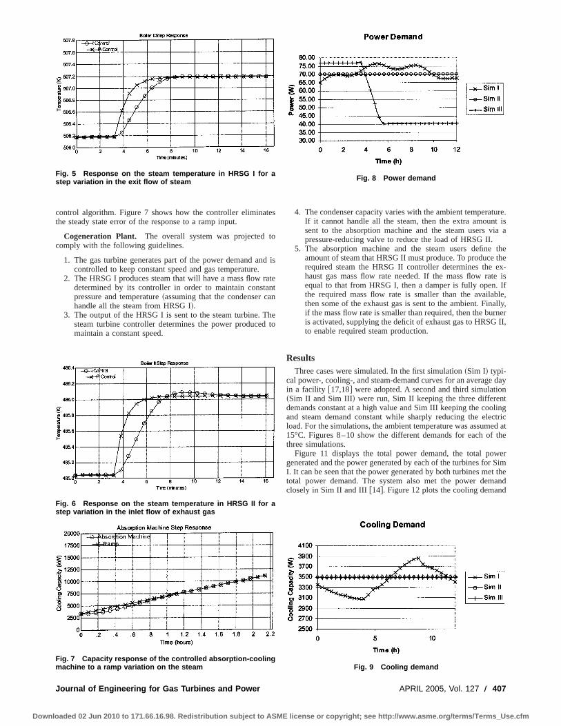
control algorithm. Figure 7 shows how the controller eliminatesthe steady state error of the response to a ramp input.

Cogeneration Plant. The overall system was projected tocomply with the following guidelines.

1. The gas turbine generates part of the power demand and iscontrolled to keep constant speed and gas temperature.

2. The HRSG I produces steam that will have a mass flow ratedetermined by its controller in order to maintain constantpressure and temperature~assuming that the condenser canhandle all the steam from HRSG I!.

3. The output of the HRSG I is sent to the steam turbine. Thesteam turbine controller determines the power produced tomaintain a constant speed.

4. The condenser capacity varies with the ambient temperature.If it cannot handle all the steam, then the extra amount issent to the absorption machine and the steam users via apressure-reducing valve to reduce the load of HRSG II.

5. The absorption machine and the steam users define theamount of steam that HRSG II must produce. To produce therequired steam the HRSG II controller determines the ex-haust gas mass flow rate needed. If the mass flow rate isequal to that from HRSG I, then a damper is fully open. Ifthe required mass flow rate is smaller than the available,then some of the exhaust gas is sent to the ambient. Finally,if the mass flow rate is smaller than required, then the burneris activated, supplying the deficit of exhaust gas to HRSG II,to enable required steam production.

ResultsThree cases were simulated. In the first simulation~Sim I! typi-

cal power-, cooling-, and steam-demand curves for an average dayin a facility @17,18# were adopted. A second and third simulation~Sim II and Sim III! were run, Sim II keeping the three differentdemands constant at a high value and Sim III keeping the coolingand steam demand constant while sharply reducing the electricload. For the simulations, the ambient temperature was assumed at15°C. Figures 8–10 show the different demands for each of thethree simulations.

Figure 11 displays the total power demand, the total powergenerated and the power generated by each of the turbines for SimI. It can be seen that the power generated by both turbines met thetotal power demand. The system also met the power demandclosely in Sim II and III@14#. Figure 12 plots the cooling demand

Fig. 5 Response on the steam temperature in HRSG I for astep variation in the exit flow of steam

Fig. 6 Response on the steam temperature in HRSG II for astep variation in the inlet flow of exhaust gas

Fig. 7 Capacity response of the controlled absorption-coolingmachine to a ramp variation on the steam

Fig. 8 Power demand

Fig. 9 Cooling demand



and the cooling capacity with respect to time for Sim I. In Sim I,the steam demand was likewise followed closely. Similarly, allloads were met in Sim II and III.

The various efficiencies adopted for cogen merit evaluation aredefined as follows:

hGT5*0

t fpGT•dt

*0t f

+

mf•dt•DH(11)

hp5*0

t f~pGT1pST!•dt

*0t f

+

mf•dt•DH(12)

h total5*0

t f~pGT1pST1pH2!•dt

*0t f

+

mf•dt•DH(13)

The efficiencies of the gas turbine, the power generation, and thetotal cogeneration plant~Eqs. 11–13! were calculated for the threesimulations. Figure 13 displays the values for Sim I.

As expected, Fig. 14 shows how the total efficiency drops fromapproximately 56% to approximately 43% when the power de-mand falls. Since the exhaust gases from the power generation arenot enough to meet the steam and cooling demand, the externalburner has to start producing hot gases at a low efficiency, there-fore, the efficiency decreases. The power and GT efficiencies tendto stay constant because the additional fuel consumed does notappear in their definition.

A fourth simulation was run were the power demand was keptconstant at 70 MW and the ambient temperature varied from 40°Cto 220°C. The controllers reacted in the following way: as theambient temperature decreased, the steam turbine produced morepower, and the gas turbine less power. This was done in order todecrease the consumption of fuel, while using the additional ex-haust gas~due to increased air inlet density at low temperatures!to drive HRSGI to greater capacity.

ConclusionsIn the present work dynamic models are used to develop a

control system for a cogeneration plant with the objective of meet-ing multiple transient demands, namely, power, heating, and cool-ing. The dynamic models vary in sophistication, but they retainone feature throughout: determining the constants that character-ize the response of the equipment to step or ramp inputs would bea relatively straightforward experimental undertaking. The modelsapply to quasy steady-state operation.

Each subsystem has its own controls, and the fast response ofthe gas turbine, coupled with the thermal storage capabilities ofthe HRSGI, allowed implementation of a LQR that minimizes fuelinput and departures of rotational speed from set point, whilemeeting the power demand. Hence, the power generated by thesteam turbine is varied so that all the exhaust gases from the gas

Fig. 10 Steam demand

Fig. 11 Distribution of the power generation for Sim I

Fig. 12 Cooling demand and capacity for Sim I

Fig. 13 Efficiencies for Sim I „typical demands …

Fig. 14 Efficiency for Sim III



turbine are used. Consequently, it is possible to eliminate the useof a duct or external burner before HRSG I most of the time.

Temporal simulations of the cogeneration system show that it ispossible to meet all demands with conventional equipment andcontrols for the load profiles employed in this study. Future workshould focus on more accurate modeling of the HRSG and on thepossibilities afforded by setting controls off-site previous toequipment shipment and installation by means of simulationssimilar to that presented here.

AcknowledgmentsThe authors gratefully acknowledge the support of the Penn

State Mechanical Engineering Department and of Chevron Texacoin the form of teaching and research assistantships.

Nomenclature

a 5 ambientA 5 active heat transfer area, m2

c 5 fluid heat capacity, kJ/s-K, specific heat, kJ/kg-KDh 5 enthalpy of vaporization, kJ/kg

h 5 specific enthalpy, kJ/kgHRSG 5 heat recovery steam generator

K, k,k1 , k2 ,

k3 5 constantsLQR 5 linear quadratic regulator

m 5 mass, kgM 5 HRSG metal mass, kg

MHRSG5 HRSG thermal mass, kg+

m 5 mass flow rate, kg/sq 5 capacity, kW

Q 5 heat transfer rate, kWr IGV 5 inlet guide vanes position.

SISO 5 single input single outputST 5 steam turbine

s 5 Laplace transform complex variableT 5 temperature, K

Tgp 5 exhaust gas temperature at evaporator exit, KTevap 5 steam evaporation temperature, K

U 5 overall heat transfer coefficientue 5 specific internal energy, kJ/kgh 5 efficiencyÃ 5 angular velocity, rad/s

Subscripts

A 5 ambientAM 5 absorption cooling machine

C 5 condenserf 5 fuel

GT 5 gas turbinee 5 exit

g 5 exhaust gasH 5 heat recovery steam generator,~HRSG!

H1 5 HRSG IH2 5 HRSG II

i 5 inletIGV 5 inlet guide vanes

l 5 liquidM 5 HRSG metal massp 5 exit of evaporator section of HRSGs 5 steam

Sat 5 saturatedv 5 vapor

References@1# Langston, L., 2002, ‘‘Electrically Charged,’’ Mech. Eng.~Am. Soc. Mech.

Eng.!, 124, No. 6.@2# Fairchild, P. D., Labinov, S. D., Zaltash, A., and Rizy, D. T., 2001, ‘‘Experi-

mental and Theoretical Study of Microturbine-Based BCHP Sytem,’’ ASMEWinter Annual Meeting, Nov.

@3# Kim, B. H., Park, Y. M., Choi, M. S., and Lee, J. W., 1996, ‘‘LQG/LTR RobustController of Cogeneration Plant for Disturbance Rejection in Electric Fre-quency and Steam Pressure,’’ Int. J. Elec. Power Energy Syst.,18, No. 4, pp.239–250.

@4# Perez-Blanco, H., and Albright, P., 2001, ‘‘Heat Recovery System ControlStrategy to Meet Multiple Transient Demands,’’ ASME Turbo Expo, Land Seaand Air 2001, June.

@5# Takahashi, K., Yasuda, T., Endoh, M., and Kurosaki, M., 2002, ‘‘Applicationof Dynamic Simulation to CAES G/T Control System Development,’’ ASMETurboExpo 2002, pp. 153–161.

@6# Sigler, J., Erickson, D., and Perez-Blanco, H., 2001, ‘‘Gas Turbine Inlet AirCooling Using Absorption Refrigeration: A Comparison Based on a CombinedCycle Process,’’ ASME Turbo Expo, Land Sea and Air 2001, New Orleans,June.

@7# http://www.fwc.com/publications/heat/heatIpdf/9604-040.pdf@8# Jeffs, E., 2002, ‘‘Siemens Offers Fast Track Maintenance to Their IPP Cli-

ents,’’ Turbomachinery Int.,43, No. 1, pp. 17–19.@9# Camporeale, S. M., Fortunato, B., and Dumas, A., 1998, ‘‘Dyanamic Modeling

and Control of Regenerative Gas Turbines,’’ ASME Int. Gas Turbine andAeroengine Congress and Exhibition, Sweden, June.

@10# Camporeale, S. M., Fortunato, B., and Mastrovito, M., 2002, ‘‘A High-FidelityReal-Time Simulation Code of Gas Turbine Dynamics for Control Applica-tions,’’ ASME Turbo Expo 2002, The Netherlands, June.

@11# Franklin, G. F., Powell, J. D., and Workman, M., 1997,Digital Control ofDynamic Systems, 3rd ed., Addison Wesley.

@12# Marlin, T. E., 2000,Design Process and Control Systems for Dynamic Perfor-mance, 2nd ed., McGraw-Hill, New York.

@13# Ogata, K., 1997,Modern Control Engineering, 3rd ed., Prentice-Hall, Engle-wood Cliffs, NJ.

@14# Sancho-Bastos, F., 2002, ‘‘Simulation and Control Strategy of a High Effi-ciency Cogeneration System to Provide Power, Heating and Cooling,’’ MSThesis, The Pennsylvania State University.

@15# Bonert, R., and Hoops, G., 1990, ‘‘Stand Alone Induction Generator WithTerminal Impedance Controller and no Turbine Controls,’’ IEEE Trans. EnergyConv.,5, No. 1, pp. 28–31.

@16# Perez-Blanco, H., and Hinojosa, L., 1999, ‘‘The Virtual Energy Laboratory~VEL!, a Didactic Graphical Simulator for Thermal Design,’’ ASME-IGTIPaper No. 99-GT-083, Turbomachinery Conference and Exposition, India-napolis.

@17# Harrison, J. A., 1999, ‘‘Electric Power Systems,’’ Prentice-Hall.@18# McQuiston, F. C., Parker, J. D., and Spitler, J. D., 2000,Heating, Ventilating,

and Air Conditioning Analysis and Design, 5th ed., Wiley, New York.



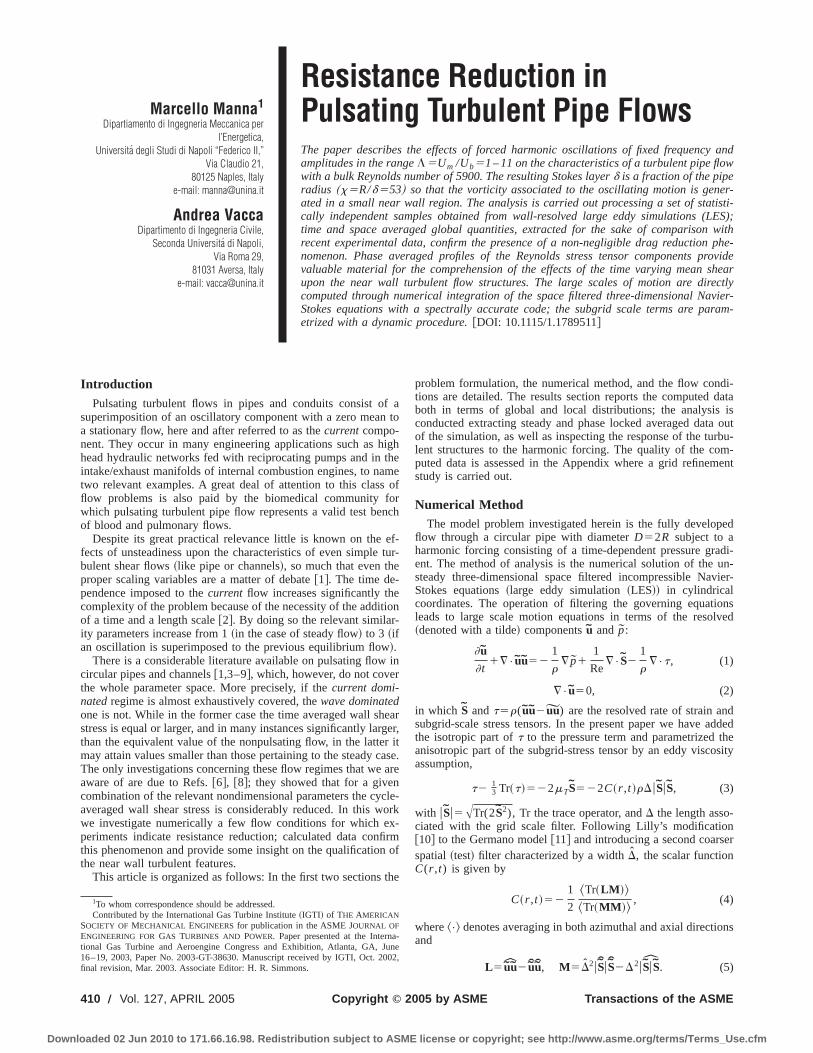
Marcello Manna1

Dipartiamento di Ingegneria Meccanica perl’Energetica,

Universita degli Studi di Napoli ‘‘Federico II,’’Via Claudio 21,

80125 Naples, Italye-mail: [email protected]

Andrea VaccaDipartimento di Ingegneria Civile,

Seconda Universita di Napoli,Via Roma 29,

81031 Aversa, Italye-mail: [email protected]

Resistance Reduction inPulsating Turbulent Pipe FlowsThe paper describes the effects of forced harmonic oscillations of fixed frequency andamplitudes in the rangeL5Um /Ub51–11 on the characteristics of a turbulent pipe flowwith a bulk Reynolds number of 5900. The resulting Stokes layerd is a fraction of the piperadius ~x5R/d553! so that the vorticity associated to the oscillating motion is gener-ated in a small near wall region. The analysis is carried out processing a set of statisti-cally independent samples obtained from wall-resolved large eddy simulations (LES);time and space averaged global quantities, extracted for the sake of comparison withrecent experimental data, confirm the presence of a non-negligible drag reduction phe-nomenon. Phase averaged profiles of the Reynolds stress tensor components providevaluable material for the comprehension of the effects of the time varying mean shearupon the near wall turbulent flow structures. The large scales of motion are directlycomputed through numerical integration of the space filtered three-dimensional Navier-Stokes equations with a spectrally accurate code; the subgrid scale terms are param-etrized with a dynamic procedure.@DOI: 10.1115/1.1789511#

IntroductionPulsating turbulent flows in pipes and conduits consist of a

superimposition of an oscillatory component with a zero mean toa stationary flow, here and after referred to as thecurrentcompo-nent. They occur in many engineering applications such as highhead hydraulic networks fed with reciprocating pumps and in theintake/exhaust manifolds of internal combustion engines, to nametwo relevant examples. A great deal of attention to this class offlow problems is also paid by the biomedical community forwhich pulsating turbulent pipe flow represents a valid test benchof blood and pulmonary flows.

Despite its great practical relevance little is known on the ef-fects of unsteadiness upon the characteristics of even simple tur-bulent shear flows~like pipe or channels!, so much that even theproper scaling variables are a matter of debate@1#. The time de-pendence imposed to thecurrent flow increases significantly thecomplexity of the problem because of the necessity of the additionof a time and a length scale@2#. By doing so the relevant similar-ity parameters increase from 1~in the case of steady flow! to 3 ~ifan oscillation is superimposed to the previous equilibrium flow!.

There is a considerable literature available on pulsating flow incircular pipes and channels@1,3–9#, which, however, do not coverthe whole parameter space. More precisely, if thecurrent domi-natedregime is almost exhaustively covered, thewave dominatedone is not. While in the former case the time averaged wall shearstress is equal or larger, and in many instances significantly larger,than the equivalent value of the nonpulsating flow, in the latter itmay attain values smaller than those pertaining to the steady case.The only investigations concerning these flow regimes that we areaware of are due to Refs.@6#, @8#; they showed that for a givencombination of the relevant nondimensional parameters the cycle-averaged wall shear stress is considerably reduced. In this workwe investigate numerically a few flow conditions for which ex-periments indicate resistance reduction; calculated data confirmthis phenomenon and provide some insight on the qualification ofthe near wall turbulent features.

This article is organized as follows: In the first two sections the

problem formulation, the numerical method, and the flow condi-tions are detailed. The results section reports the computed databoth in terms of global and local distributions; the analysis isconducted extracting steady and phase locked averaged data outof the simulation, as well as inspecting the response of the turbu-lent structures to the harmonic forcing. The quality of the com-puted data is assessed in the Appendix where a grid refinementstudy is carried out.

Numerical MethodThe model problem investigated herein is the fully developed

flow through a circular pipe with diameterD52R subject to aharmonic forcing consisting of a time-dependent pressure gradi-ent. The method of analysis is the numerical solution of the un-steady three-dimensional space filtered incompressible Navier-Stokes equations~large eddy simulation~LES!! in cylindricalcoordinates. The operation of filtering the governing equationsleads to large scale motion equations in terms of the resolved~denoted with a tilde! componentsu and p:

]u

]t1¹•uu52

1

r¹ p1

1

Re¹•S2

1

r¹•t, (1)

¹•u50, (2)

in which S andt5r(uu2uu) are the resolved rate of strain andsubgrid-scale stress tensors. In the present paper we have addedthe isotropic part oft to the pressure term and parametrized theanisotropic part of the subgrid-stress tensor by an eddy viscosityassumption,

t213 Tr~t!522mTS522C~r ,t !rDuSuS, (3)

with uSu5ATr(2S2), Tr the trace operator, andD the length asso-ciated with the grid scale filter. Following Lilly’s modification@10# to the Germano model@11# and introducing a second coarserspatial~test! filter characterized by a widthD, the scalar functionC(r ,t) is given by

C~r ,t !521

2

^Tr~LM !&

^Tr~MM !&, (4)

where^•& denotes averaging in both azimuthal and axial directionsand

L5uu2 uu, M5D2u Su S2D2uSu S. (5)


SOCIETY OF MECHANICAL ENGINEERSfor publication in the ASME JOURNAL OFENGINEERING FOR GAS TURBINES AND POWER. Paper presented at the Interna-tional Gas Turbine and Aeroengine Congress and Exhibition, Atlanta, GA, June16–19, 2003, Paper No. 2003-GT-38630. Manuscript received by IGTI, Oct. 2002,final revision, Mar. 2003. Associate Editor: H. R. Simmons.



Sharp Fourier cutoff is used as both grid and test filter in stream-wise and azimuthal directions, while no test filtering is performedin the radial direction. The test filter width is such thatD/D52.Details on the potential and limitations of the dynamic eddy vis-cosity procedure for both steady and unsteady channel flow prob-lems are discussed in great depth in Refs.@9#, @12#, and will beomitted.

The governing equations~1! and~2! have been solved using theinitial value solver developed and validated in Ref.@13#. The nu-merical method relies on a spectral Chebyshev multidomain algo-rithm for the inhomogeneous~radial! direction and Fourier de-composition for the homogeneous~streamwise and azimuthal!ones. Time integration is carried out with a Crank-Nicolsonscheme for the viscous terms. The nonlinear convective terms, inskew-symmetric form, are treated explicitly with an Adams-Bashforth scheme. Periodic boundary conditions are applied instreamwise and azimuthal directions, and no-slip boundary condi-tions at the solid walls.

Problem FormulationIn what follows, we shall denote withu, v, w the streamwise

~z!, radial ~r!, and azimuthal~u! velocity components, respec-tively. As customary in equilibrium computations the flow is as-sumed periodic in the streamwise~and obviously azimuthal! di-rection, with a periodicity lengthLz equal to 4pR. This value hasbeen shown, in the steady case, to be sufficient for the streamwisetwo point correlations of the velocity components to drop to zeroat the largest separation distance@14#. In the unsteady case, espe-cially when a drag reduction phenomenon is expected, theLzvalue should be increased; we have thus computed theL51 andL511 cases with different lengths, viz.Lz54pR andLz56pR,respectively.

The flow is driven in the streamwise direction by a sinusoidaloscillatory in time external pressure gradient of appropriate meanvalue, amplitude, and pulsationDp/Lz@11a cos(vt)#. The con-stant part of the pressure gradientDp/Lz , together with the am-plitude aDp/Lz and the pulsationv of the oscillation, were se-lected in order to achieve flow conditions in full similarity withthe experimental setup of Ref.@8#. As anticipated in the Introduc-tion, pulsating flows are fully characterized by three nondimen-sional parameters, namely

Reb5UbD

n, Red5

Umd

n, L5

Um

Ub,

whered52n/v is the Stokes layer thickness,n the kinematic vis-cosity, Ub the cross-sectional mean velocity, andUm the maxi-mum value of the oscillatory flow at the center of the pipe. Othertriplets are of course possible@1,8#. For the sake of simplicity, i.e.,to closely follow the experimental setup of Ref.@8#, we shall alsorefer to the following additional parameterx5R/d. Obviouslyx5Reb L/(2 Red). For oscillating flow with a Red,200 andR/d.10 the velocity field follows very closely the theoretical Stokesdistribution @2#; this is usually referred to as the laminar regime.Increasing the Reynolds number up to the critical value of Red;550, small perturbations appear superimposed to the Stokesflow ~disturbed laminar regime! @15#. Experimental and numericaldata indicate the occurrence of turbulent flow conditions in thedecelerating phase of the cycle when Red.1000 ~intermittentlyturbulent regime!; fully turbulent flows across the whole cycleoccur instead for values of Red larger than 3500@16#. Accordingto Ref. @8# there are four main regimes that completely character-ize this three-dimensional state space, namely

current dominatedL<1 Hhigh-frequency regimes Red,1000

low-frequency regimes Red.1000,

wave dominatedL>10 Hhigh-frequency regimes Red,1000

low-frequency regimes Red.1000.

Here and after we shall assume that thecurrent flow is turbulent,that is, Reb.2300. Unlike the oscillating flow for which the sta-bility region is defined by a single value of Red (Red,cr;550 forx.10!, in the case of pulsating pipe flows the transition condi-tions are defined by a combination of both Red and Reb @8#. Ex-perimental data@6,8# indicate that in the wave dominated regimeand for Red,Red,cr a drag reduction phenomenon occur. Thus wehave focused our attention on three flow regimes detailed in Table1. In the last case we expect drag reduction. Both unsteady con-ditions are characterized byx553.

ResultsThe calculations were performed over a total integration time of

330 nondimensional unitstUb /D. Data reduction was carried outprocessing 160 statistically independent samples separated in timeby 0.4 nondimensional time units, both in the steady and unsteadycases. All quantities are space averaged in the homogeneousz andu directions; furthermore, time and/or phase averaging is appliedto collect the statistics. In what follows, we shall indicate with anoverline or capital letters the time and space averaged quantities,with ^•& the phase and space averaged quantities and with primethe perturbation from their time averages.

We begin this section presenting in Table 2 some global quan-tities, computed for the steady and oscillating flow conditions; alldata are space and time averaged. As discussed in the previoussection, the simulations are carried out with either a constant ortime varying forcing term; thus the effective flow rates and bulk orcenterline Reynolds numbers are a results of the calculations andas such cannot be round numbers. The differences between thecomputed values and the expected ones are of double nature, viz.numerical and physical. In the Appendix we provide exhaustiveevidence that the former, i.e., the uncertainties associated with themodeled subgrid terms, are comfortably small, so that the dragreduction phenomena can be evaluated with good confidence.

Returning to the global values of Table 2, we first notice thatthe ratioUcl /Ub between the centerline and bulk velocities is inboth cases very close to the steady pipe value. This indicates that,at least in an average sense, the velocity profiles are somewhatsimilar. As it will be shown later, the radial distributions of themean velocity still retain a clearly turbulent shape, with a welldefined logarithmic region. The displacement and momentumthicknesses defined as

d* ~D2d* !52E0

RS 12u~r !

UcD rdr ,

Table 1 Flow regimes investigated

Reb Red L

Steady flow 5900 0 0Current dominated 6100 56 1Wave dominated 5546 572 11

Table 2 Mean flow quantities

L Reb Ucl /Ub d* /R u* /R H

0 5900 1.32 0.129 0.069 1.871 6100 1.32 0.129 0.069 1.88

11 5546 1.29 0.121 0.059 2.05

L Reb Ret d1 Um /Ucl Cf /CfB

0 5900 192 1.061 6100 194 3.67 0.76 0.90

11 5546 160 3.01 8.50 0.73



u* ~D2u* !52E0

RS 12u~r !

UcD u~r !

Ucrdr , H5

d*

u*

also show insignificant variations, while their ratio, i.e., the shapefactorH is seen to increase of about 9% in the caseL511, and toremain equal to the steady value in the caseL51. Recalling thatthe laminar value is 3.37 we may already foresee the occurrenceof some resistance reduction; in fact, the skin friction coefficientCf5tw/1/2rUb

2 is smaller than the corresponding Blasius value(Cf

B50.079 Reb21/4) for both unsteady cases~10% for L51 and

27% forL511!. This is in accordance with the experimental data@8,6#.

The radial distribution of the time averaged mean velocity isshown in inner coordinates in Fig. 1 for the three cases. In whatfollows we shall indicate withy5(R2r )/R the distance from thesolid wall. The wall values used for the normalization are space~in the homogeneous directions! and time averaged. The deviationfrom the logarithmic distribution u151/k ln(y1)1B ~withk50.41 andB55.5) is similar to the one observed in the experi-ments and calculations reported in Ref.@14#.

In the current-dominated case the profile essentially collapseson the steady distribution. This is a nontrivial result, since forL.1 the amplitude of the velocity oscillation becomes greaterthan the local velocity close to the wall and thus flow reversaloccurs. The somewhat surprising insensitivity of the mean flowprofile to the imposed oscillations, in the caseL;1, has not yetreceived, in the author’s opinion, a convincing explanation. Tuet al. @3# have argued that whenever the oscillating frequencyf o5D/(TUb) is significantly below the bursting frequencyf b thereshould be no effect of the pulsation on the mean velocity profile.In view of this argument, and since our data do not satisfy theircriterion (f o;0.61. f b;0.2 @3#!, we would expect to observesome modifications in theu radial distributions, which is appar-ently not the case. The absence of any significant departure fromthe steady condition, in the current dominated high-frequency re-gime, has also been observed in plane channel geometries bothexperimentally@1# and numerically@9# in similar flow conditions(Recl58500, Um /Ucl50.64, d158.1 in Ref. @1# and Recl

57250,Um /Ucl50.75,d154.4 in Ref.@9#!.The oscillating case withL511 still presents a logarithmic re-

gion with a slope 1/k essentially equal to the corresponding steadyslope but characterized by an upward shift. This shift and theconsequent increase of the viscous sublayer thickness is typical ofdrag reducing flows.

Figure 2 shows, in inner coordinates, the radial distribution ofthe root-mean-square values of the fluctuating velocity compo-nentsu8u81, n8n81, andw8w81, for both oscillating cases. Alsoreported in the same figure are the steady distributions togetherwith reference experimental and numerical data@1,9#. For the

lowest value of the amplitudeL51 all components show a goodcorrespondence with the steady profiles, except for the maximumvalue of u8u81. The largest difference is, however, small, i.e.,;3%. The above picture changes quite substantially in theL511case; on a general ground we note that the net effect of the largeamplitude unsteady forcing on the normal stresses extends up toy1;50, and basically consists of a reduction of all components.There are no experimental data available to corroborate thesetrends.

In Fig. 3 the space and time averaged data of the turbulent~resolved and subgrid-scale stress! and viscous stresses are re-ported for all simulations, in inner coordinates. The current domi-nated case does not show any significant departure from thesteady flow distribution, either of the turbulent shear stressu8n81

or of the viscous onedu1/dy1. This is in accordance with theglobal data previously discussed. In the wave dominated regime,on the other hand, a remarkable reduction ofu8n81 across thewhole pipe radius occurs. The inner coordinates representationhighlights that the turbulent stress reduction is uniform, i.e., thewhole wall layer is witnessing a weaker response of the turbu-lence to the unsteady forcing. However,u8n81 is not at all neg-ligible and thus the flow is definitely not in a reverse transitionstage; note that neither is the extent of the overlap region substan-

Fig. 1 Mean velocity profiles

Fig. 2 Mean turbulent intensities; d experiments †1‡;h LES †9‡

Fig. 3 Turbulent and viscous shear stress



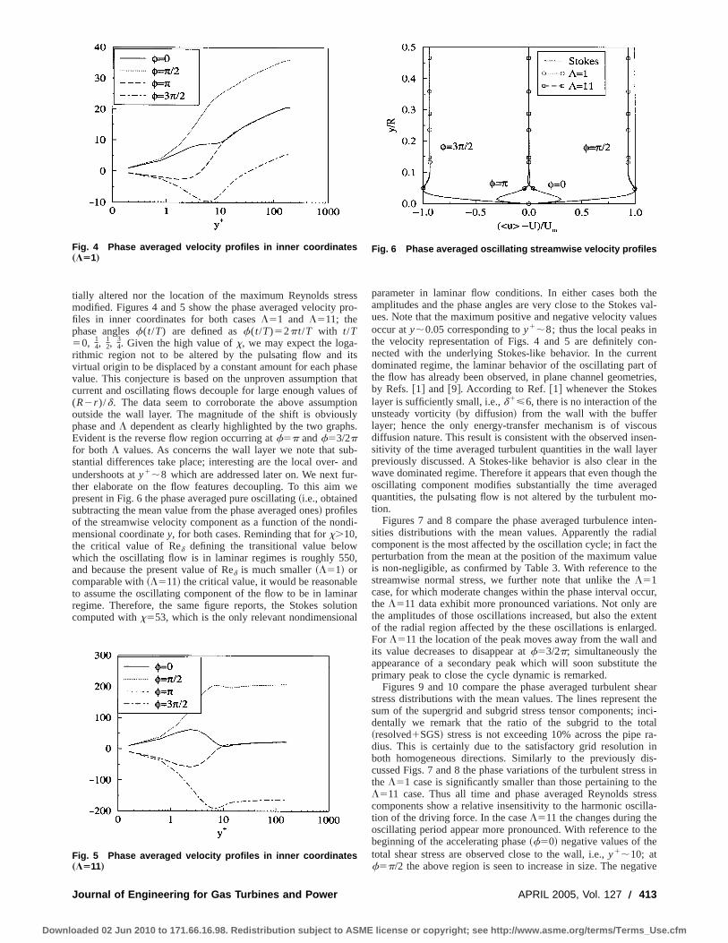
tially altered nor the location of the maximum Reynolds stressmodified. Figures 4 and 5 show the phase averaged velocity pro-files in inner coordinates for both casesL51 and L511; thephase anglesf(t/T) are defined asf(t/T)52pt/T with t/T50, 1

4,12,

34. Given the high value ofx, we may expect the loga-

rithmic region not to be altered by the pulsating flow and itsvirtual origin to be displaced by a constant amount for each phasevalue. This conjecture is based on the unproven assumption thatcurrent and oscillating flows decouple for large enough values of(R2r )/d. The data seem to corroborate the above assumptionoutside the wall layer. The magnitude of the shift is obviouslyphase andL dependent as clearly highlighted by the two graphs.Evident is the reverse flow region occurring atf5p andf53/2pfor both L values. As concerns the wall layer we note that sub-stantial differences take place; interesting are the local over- andundershoots aty1;8 which are addressed later on. We next fur-ther elaborate on the flow features decoupling. To this aim wepresent in Fig. 6 the phase averaged pure oscillating~i.e., obtainedsubtracting the mean value from the phase averaged ones! profilesof the streamwise velocity component as a function of the nondi-mensional coordinatey, for both cases. Reminding that forx.10,the critical value of Red defining the transitional value belowwhich the oscillating flow is in laminar regimes is roughly 550,and because the present value of Red is much smaller~L51! orcomparable with~L511! the critical value, it would be reasonableto assume the oscillating component of the flow to be in laminarregime. Therefore, the same figure reports, the Stokes solutioncomputed withx553, which is the only relevant nondimensional

parameter in laminar flow conditions. In either cases both theamplitudes and the phase angles are very close to the Stokes val-ues. Note that the maximum positive and negative velocity valuesoccur aty;0.05 corresponding toy1;8; thus the local peaks inthe velocity representation of Figs. 4 and 5 are definitely con-nected with the underlying Stokes-like behavior. In the currentdominated regime, the laminar behavior of the oscillating part ofthe flow has already been observed, in plane channel geometries,by Refs.@1# and @9#. According to Ref.@1# whenever the Stokeslayer is sufficiently small, i.e.,d1<6, there is no interaction of theunsteady vorticity~by diffusion! from the wall with the bufferlayer; hence the only energy-transfer mechanism is of viscousdiffusion nature. This result is consistent with the observed insen-sitivity of the time averaged turbulent quantities in the wall layerpreviously discussed. A Stokes-like behavior is also clear in thewave dominated regime. Therefore it appears that even though theoscillating component modifies substantially the time averagedquantities, the pulsating flow is not altered by the turbulent mo-tion.

Figures 7 and 8 compare the phase averaged turbulence inten-sities distributions with the mean values. Apparently the radialcomponent is the most affected by the oscillation cycle; in fact theperturbation from the mean at the position of the maximum valueis non-negligible, as confirmed by Table 3. With reference to thestreamwise normal stress, we further note that unlike theL51case, for which moderate changes within the phase interval occur,the L511 data exhibit more pronounced variations. Not only arethe amplitudes of those oscillations increased, but also the extentof the radial region affected by the these oscillations is enlarged.For L511 the location of the peak moves away from the wall andits value decreases to disappear atf53/2p; simultaneously theappearance of a secondary peak which will soon substitute theprimary peak to close the cycle dynamic is remarked.

Figures 9 and 10 compare the phase averaged turbulent shearstress distributions with the mean values. The lines represent thesum of the supergrid and subgrid stress tensor components; inci-dentally we remark that the ratio of the subgrid to the total~resolved1SGS! stress is not exceeding 10% across the pipe ra-dius. This is certainly due to the satisfactory grid resolution inboth homogeneous directions. Similarly to the previously dis-cussed Figs. 7 and 8 the phase variations of the turbulent stress inthe L51 case is significantly smaller than those pertaining to theL511 case. Thus all time and phase averaged Reynolds stresscomponents show a relative insensitivity to the harmonic oscilla-tion of the driving force. In the caseL511 the changes during theoscillating period appear more pronounced. With reference to thebeginning of the accelerating phase~f50! negative values of thetotal shear stress are observed close to the wall, i.e.,y1;10; atf5p/2 the above region is seen to increase in size. The negative

Fig. 4 Phase averaged velocity profiles in inner coordinates„LÄ1…

Fig. 5 Phase averaged velocity profiles in inner coordinates„LÄ11…

Fig. 6 Phase averaged oscillating streamwise velocity profiles



peak value position shifts towards the pipe core. The oscillationsweaken considerably fory1.30; this behavior is also shared bythe L51 case.

In Figs. 11 and 12 the temporal evolutions of both oscillatingstreamwise velocity and Reynolds stress tensor components at theposition of maximumu8u8 are shown; the data, normalized withthe time mean values, are presented as a function of the phaseanglef. As already evident from Fig. 6, theu2u fluctuation hasan almost perfect harmonic shape, with ap/2 phase shift withrespect to the driving forcing term. There is no appreciable effectof the L parameter upon the shape of the profiles, except, ofcourse, for the amplitudes which roughly differ by a factor 10.The scaling factor is not exactly 11 because the graphs pertain tothe peak locations ofu8u8 which occur at slightly different radialpositions~see caption of Fig. 11!. Conversely, the Reynolds stressprofiles show the appearance of temporal modes with higher~than1! frequency contents and non-negligible amplitudes, which in-crease withL. Note the asymmetry of the positive and negativepeaks. In addition there is considerable variation in the phase

angles for the twoL cases. Thus the amplitude increase of theforcing induces a different response of the second-order momentsdespite the integral time scale of the mean flows is unchanged. Wecan therefore conclude that the response of the smaller turbulencescales to the external forcing is affected by the amplitude of the

Fig. 7 Phase averaged „ … and mean „ … turbulent in-tensities for LÄ1

Fig. 8 Phase averaged „ … and mean „ … turbulent in-tensities for LÄ11

Table 3 Normal stress phase variation at y¿Ä13 „LÄ1… andy¿Ä14.8 „LÄ11…

L51

Phase angle 0 p/2 p 3p/2

u8u8 1.9% 25.7% 22.0% 5.5%

v8v8 10.6% 4.7% 211.0% 26.4%

w8w8 24.9% 3.3% 6.0% 22.7%

L511

Phase angle 0 p/2 p 3p/2

u8u8 11.3% 1.9% 211.2% 23.6%

v8v8 13.0% 7.2% 13.5% 211.8%

w8w8 0% 24.7% 22.6% 6.7%



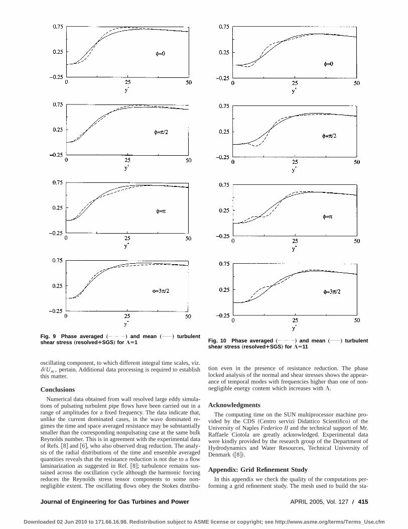
oscillating component, to which different integral time scales, viz.d/Um , pertain. Additional data processing is required to establishthis matter.

ConclusionsNumerical data obtained from wall resolved large eddy simula-

tions of pulsating turbulent pipe flows have been carried out in arange of amplitudes for a fixed frequency. The data indicate that,unlike the current dominated cases, in the wave dominated re-gimes the time and space averaged resistance may be substantiallysmaller than the corresponding nonpulsating case at the same bulkReynolds number. This is in agreement with the experimental dataof Refs.@8# and@6#, who also observed drag reduction. The analy-sis of the radial distributions of the time and ensemble averagedquantities reveals that the resistance reduction is not due to a flowlaminarization as suggested in Ref.@8#; turbulence remains sus-tained across the oscillation cycle although the harmonic forcingreduces the Reynolds stress tensor components to some non-negligible extent. The oscillating flows obey the Stokes distribu-

tion even in the presence of resistance reduction. The phaselocked analysis of the normal and shear stresses shows the appear-ance of temporal modes with frequencies higher than one of non-negligible energy content which increases withL.

AcknowledgmentsThe computing time on the SUN multiprocessor machine pro-

vided by the CDS~Centro servizi Didattico Scientifico! of theUniversity of NaplesFederico IIand the technical support of Mr.Raffaele Ciotola are greatly acknowledged. Experimental datawere kindly provided by the research group of the Department ofHydrodynamics and Water Resources, Technical University ofDenmark~@8#!.

Appendix: Grid Refinement StudyIn this appendix we check the quality of the computations per-

forming a grid refinement study. The mesh used to build the sta-

Fig. 9 Phase averaged „ … and mean „ … turbulentshear stress „resolved ¿SGS… for LÄ1 Fig. 10 Phase averaged „ … and mean „ … turbulent

shear stress „resolved ¿SGS… for LÄ11



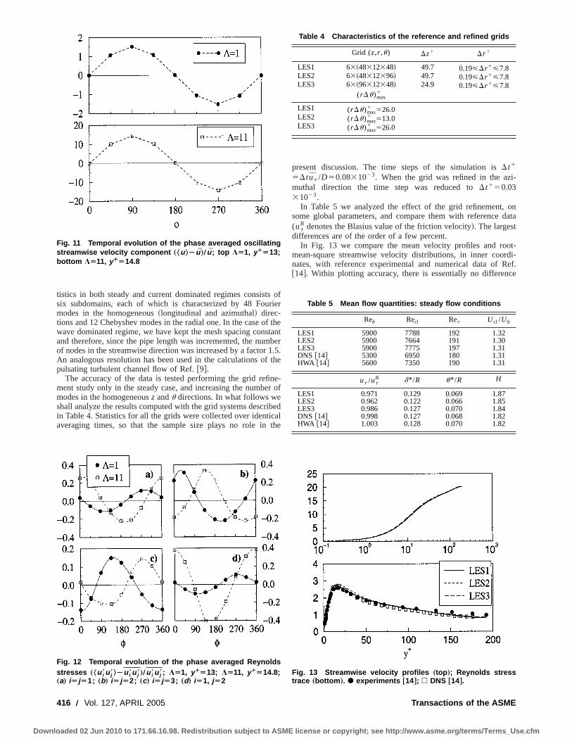
tistics in both steady and current dominated regimes consists ofsix subdomains, each of which is characterized by 48 Fouriermodes in the homogeneous~longitudinal and azimuthal! direc-tions and 12 Chebyshev modes in the radial one. In the case of thewave dominated regime, we have kept the mesh spacing constantand therefore, since the pipe length was incremented, the numberof nodes in the streamwise direction was increased by a factor 1.5.An analogous resolution has been used in the calculations of thepulsating turbulent channel flow of Ref.@9#.

The accuracy of the data is tested performing the grid refine-ment study only in the steady case, and increasing the number ofmodes in the homogeneousz andu directions. In what follows weshall analyze the results computed with the grid systems describedin Table 4. Statistics for all the grids were collected over identicalaveraging times, so that the sample size plays no role in the

present discussion. The time steps of the simulation isDt1

5Dtut /D50.0831023. When the grid was refined in the azi-muthal direction the time step was reduced toDt150.0331023.

In Table 5 we analyzed the effect of the grid refinement, onsome global parameters, and compare them with reference data(ut

B denotes the Blasius value of the friction velocity!. The largestdifferences are of the order of a few percent.

In Fig. 13 we compare the mean velocity profiles and root-mean-square streamwise velocity distributions, in inner coordi-nates, with reference experimental and numerical data of Ref.@14#. Within plotting accuracy, there is essentially no difference

Fig. 11 Temporal evolution of the phase averaged oscillatingstreamwise velocity component „Šu ‹Àu …Õu ; top LÄ1, y¿Ä13;bottom LÄ11, y¿Ä14.8

Fig. 12 Temporal evolution of the phase averaged Reynoldsstresses „Šu i8u j8‹Àu i8u j8…Õu i8u j8; LÄ1, y¿Ä13; LÄ11, y¿Ä14.8;„a… iÄ jÄ1; „b… iÄ jÄ2; „c… iÄ jÄ3; „d… iÄ1, jÄ2

Fig. 13 Streamwise velocity profiles „top …; Reynolds stresstrace „bottom …. d experiments †14‡; h DNS †14‡.

Table 4 Characteristics of the reference and refined grids

Grid (z,r ,u) Dz1 Dr 1

LES1 63~48312348! 49.7 0.19<Dr 1<7.8LES2 63~48312396! 49.7 0.19<Dr 1<7.8LES3 63~96312348! 24.9 0.19<Dr 1<7.8

(rDu)max1

LES1 (rDu)max1 526.0



Table 5 Mean flow quantities: steady flow conditions

Reb Recl Ret Ucl /Ub

LES1 5900 7788 192 1.32LES2 5900 7664 191 1.30LES3 5900 7775 197 1.31DNS @14# 5300 6950 180 1.31HWA @14# 5600 7350 190 1.31

ut /utB d* /R u* /R H

LES1 0.971 0.129 0.069 1.87LES2 0.962 0.122 0.066 1.85LES3 0.986 0.127 0.070 1.84DNS @14# 0.998 0.127 0.068 1.82HWA @14# 1.003 0.128 0.070 1.82



between LES1 and LES3, while LES2 differs from the other twoin the wall layer by some small amount~the largest difference is2.5% aty1;15). We have therefore good confidence in the qual-ity of the present results.

Figure 14 depicts, in inner coordinates, the viscous stress, theresolved1SGS turbulent stress along with the total ones~top halffigure!, together with the DNS data of Ref.@14#. Shown also arethe subgrid stress distributions~bottom half!; note the differentscale on they axis. Interesting is the expected decrease of the SGSpart in the outer layer when the streamwise resolution is increased~LES1 versus LES3! and the reverse phenomenon characterizingthe azimuthally more resolved grid~LES2!. This is an effect of thecylindrical coordinates which puts into evidence the role of thestreamwise box size whenr→0; conversely in the buffer layerthere is clearly a demand for an enhanced resolution to properlydescribe the streaks dynamics.

From the foregoing we may argue that the multiple scale char-acteristics of this kind of wall bounded shear flows would bebetter accounted for, in a LES framework, with a nonconformingtechnology. Work is in progress in this direction.

Nomenclature

Dimensional Quantities

d5A2n/v 5 Stokes layer thicknessd* 5 displacement thicknessD 5 filter sizek 5 von Karman constant

mT 5 turbulent viscosityn 5 kinematic viscosityp 5 static pressureu 5 momentum thicknessr 5 radial coordinate

ru 5 azimuthal coordinateR, D 5 pipe radius, diameter

r 5 fluid densityS 5 rate of strain tensort 5 time coordinate

T 5 oscillating periodt 5 subgrid scale stress tensor

uz , u, u1 5 axial velocity componentur , v, u2 5 radial velocity component

uu , w, u3 5 azimuthal velocity componentu 5 velocity vector

ut 5 wall friction velocityy 5 distance from the wallz 5 axial coordinate

v52p/T 5 oscillating frequency

Nondimensional Quantities

Cf 5 friction coefficientf52pt/T 5 phase angle

H 5 shape factorL5Um /Ub 5 amplitude oscillation parameterReb5UbD/n 5 bulk Reynolds numberRet5utR/n 5 Reynolds number

Red5Umd/n 5 oscillating Reynolds numberx5R/d 5 Stokes parameter

Subscripts

b 5 bulk, area averaged valuecl 5 centerline valuem 5 maximum oscillatory value atr 50w 5 wall value

Superscripts

1 5 wall coordinates8 5 fluctuating componentB 5 Blasius value

Averaging Operators

˙ 5 time and space averaged^•& 5 phase and space averaged

˙ 5 resolved quantity

References@1# Tardu, S. F., Binder, G., and Blackwelder, R. F., 1994, ‘‘Turbulent Channel

Flow With Large-Amplitude Velocity Oscillations,’’ J. Fluid Mech.,267, pp.109–151.

@2# Akhavan, R., Kamm, R. D., and Shapiro, A. H., 1991, ‘‘An Investigation ofTransition to Turbulence in Bounded Oscillatory Stokes Flows Part 1. Experi-ments,’’ J. Fluid Mech.,225, pp. 395–442.

@3# Tu, S. W., and Ramaprian, B. R., 1983, ‘‘Fully Developed Periodic TurbulentPipe Flow. Part 1. Main Experimental Results and Comparison With Predic-tions,’’ J. Fluid Mech.,137, pp. 31–58.

@4# Tu, S. W., and Ramaprian, B. R., 1983, ‘‘Fully Developed Periodic TurbulentPipe Flow. Part 2. The Detailed Structure of the Flow,’’ J. Fluid Mech.,137,pp. 59–81.

@5# Mao, Z. X., and Hanratty, T. J., 1986, ‘‘Studies of the Wall Shear Stress in aTurbulent Pulsating Pipe Flow,’’ J. Fluid Mech.,170, pp. 545–565.

@6# Mao, Z. X., and Hanratty, T. J., 1994, ‘‘Influence of Large-Amplitude Oscil-lations on Turbulent Drag,’’ AIChE J.,40~10!, pp. 1601–1610.

@7# Tardu, S. F., and Binder, G., 1993, ‘‘Wall Shear Stress Modulation in UnsteadyTurbulent Channel Flow With High Imposed Frequencies,’’ Phys. Fluids,5,pp. 2028–2034.

@8# Lodahl, C. R., Sumer, B. M., and Fredosoe, J., 1998, ‘‘Turbulent CombinedOscillatory Flow and Current in a Pipe,’’ J. Fluid Mech.,373, pp. 313–348.

@9# Scotti, A., and Piomelli, U., 2001, ‘‘Numerical Simulation of Pulsating Turbu-lent Channel Flow,’’ Phys. Fluids,13~5!, pp. 1367–1384.

@10# Lilly, D. K., 1992, ‘‘A Proposed Modification of the Germano Subgrid-ScaleClosure Method,’’ Phys. Fluids,4~3!, pp. 633–635.

@11# Germano, M., Piomelli, U., Moin, P., and Cabot, W. H., 1991, ‘‘A DynamicSubgrid Scale Eddy Viscosity Model,’’ Phys. Fluids,3, pp. 1760–1767.

@12# Piomelli, U., 1993, ‘‘High Reynolds Number Calculations Using the DynamicSubgrid Scale Stress Model,’’ Phys. Fluids,5~6!, 1484–1490.

@13# Manna, M., and Vacca, A., 1999, ‘‘An Efficient Method for the Solution of theIncompressible Navier-Stokes Equations in Cylindrical Geometries,’’ J. Com-put. Phys.,151, pp. 563–584.

@14# Eggels, J. G. M., Unger, F., Weiss, M. H., Westerweel, J., Adrian, R. J.,Friedrich, R., and Nieuwstadt, F. T. M., 1994, ‘‘Fully Developed TurbulentPipe Flow: A Comparison Between Direct Numerical Simulation and Experi-ments,’’ J. Fluid Mech.,268, pp. 175–209.

@15# Hino, M., Sawamoto, M., and Takasu, S., 1976, ‘‘Experiments on Transition toTurbulence in an Oscillatory Pipe Flow,’’ J. Fluid Mech.,75, pp. 193–207.

@16# Jensen, B., Sumer, B., and Fredosoe, J., 1989, ‘‘Turbulent OscillatoryBoundary Layers at High Reynolds Number,’’ J. Fluid Mech.,206, pp. 265–297.

Fig. 14 Turbulent and viscous stresses „top …; SGS stresses„bottom …; h DNS †14‡



Hyeong-Joon Ahne-mail: [email protected]

Eric H. Maslene-mail: [email protected]

Tetsuya Iwasakie-mail: [email protected]

Department of Mechanical and AerospaceEngineering,

University of Virginia,122 Engineer’s Way,

Charlottesville, VA 22904-4746

Feasibility Analysis for theRotordynamic Performance ofAPI617The rotordynamic performance of API 617 standards provides two primary requirements.First, the standard stipulates system damping near the expected operating speed range.Second, the standard requires a specific bound of the worst case unbalance response. Theproblem this poses for machine designers is (1) feasibility: can bearings be designed fora given rotor to meet API 617 and (2) if so, how can these bearings be designed? Ourprimary effort in this research is to convert the API requirements to a control designobjective for a bearing. This permits direct assessment of the feasible design problem aswell as providing a means to synthesize optimal bearing dynamics. In addition to provid-ing synthesis of magnetic bearings, the resulting bearing transfer functions give directguidance to selection of more conventional fluid film or rolling element bearings.@DOI: 10.1115/1.1789492#

IntroductionThe rotordynamic performance of API 617 standards provides

two primary requirements. First, the standard stipulates systemdamping near the expected operating speed range. This takes theform of a combination of damping requirements and separationmargins, depending on where the system critical speeds lie rela-tive to the operating range. Second, the standard requires a spe-cific bound on the worst case unbalance response.

The problem this poses for machine designers is~1! feasibility:can bearings be designed for a given rotor to meet API 617 and~2! if so, how can these bearings be designed? This paper exam-ines the feasibility problem. One possible approach to assessingfeasibility would be to pick bearings, to model the final machine~including bearings!, and to assess the resulting API 617 compli-ance. The problem with this approach is that the choice of bearingdictates the outcome and it may be difficult to select an optimalbearing for API 617. Consequently, failure of this test does notimply non-feasibility.

An alternative approach is to convert the API requirements to acontrol design problem. With this approach, it is not necessary topredesign or preselect the bearings: we can determine directlywhether a bearing set exists that satisfies the control design prob-lem. In this case, feasibility will not assure that a given type ofbearing~fluid film, rolling element, . . . ! can meet the API stan-dard, but it does imply that the requirement can be met throughsome mechanism~perhaps a magnetic bearing!.

Some Tools. Constructing this control design problem re-quires three important mathematical tools:H` norms @1#,m-analysis@2#, andm synthesis@3#. We present here a very briefsynopsis: the full story can be found in Ref.@4#.

The H` norm measures generalized peak of gain. Assume adynamic systemy5G(s;N) f . The response is a function of com-plex frequency,s, and may also depend on parameter~s! N ~whichmight be the rotor spin rate, for instance!. At any givens5 j v, thesteady-state responsey to sinusoidal inputf is computed by evalu-ating the matrix functionG( j v). BecauseG is a matrix, the gainfrom f to y depends on the direction off. A bound on how largeycan be for a boundedf is the maximum singular value

s„G( j v;N)… @5#. The maximum singular value can be viewed asa composite summary of each of the individual transfer functionswhich constituteG.

TheH` norm ofG(s;N) is the largest maximum singular valueof G( j v;N) when v ranges from zero to infinity. IfG were ascalar function ofs, then theH` norm of G(s) would be thehighest point on the Bode magnitude plot ofG(s).

m-analysis considers the stability problem where some stablesystemG(s) is connected to some other uncertain~but stable!systemW(s)D, as shown in Fig. 1. Here,W(s) describes theexpected frequency response character of the uncertain systemwhile D is a bound on its gain. For instance, if a rotor is connectedto a seal with unknown damping:25 Nsec/m,Cseal,25 Nsec/m, thenG(s) would contain the nominal damping~10Nsec/m!, W(s) might be the transfer function 15s, andD wouldbe 61.

Now, ask: Is the closed loop system stable for all possibleD,whereD is bounded~typically by 61!? Using a very central resultof control theory called the small gain theorem@6#, m-analysisreturns a figure of merit,m. If m,1, then the system is stable forall allowed values ofD while if m.1, it may not be.

Finally, m-synthesis constructs a controller for an uncertainplant (G(s) connected toW(s)D) so that the resulting closed loopsystem will be stable for all possibleD. Therefore, the resultingclosed-loop system isrobust to uncertainties described byD.

The Feasibility Problem. The unbalance response require-ment is exactly a formalH` performance measure, but the sepa-ration margin requirement is not analytic so it is not simple todirectly formulate this requirement as a linear system analysisproblem. In this paper, the separation margin requirement is re-placed by a pole placement problem: relatively large dampingnear the operating range. The pole placement problem can beapproximated as a robust stability problem with frequency shapeduncertain modal damping. Since the unbalance response require-ment can already be expressed as anH` problem, the two API 617requirements can be cast as a singlem-analysis problem. Thispermits direct assessment of the feasible design problem and alsoprovides a means to synthesize optimal bearing dynamics. In ad-dition to providing synthesis of magnetic bearings, the resultingbearing transfer functions may give direct guidance to selection ofmore conventional fluid film or rolling element bearings.

The API 617 Standards†7‡Given a rotor-bearing system with a probe at a certain~impor-

tant! location, one can experimentally find the vibration amplitude




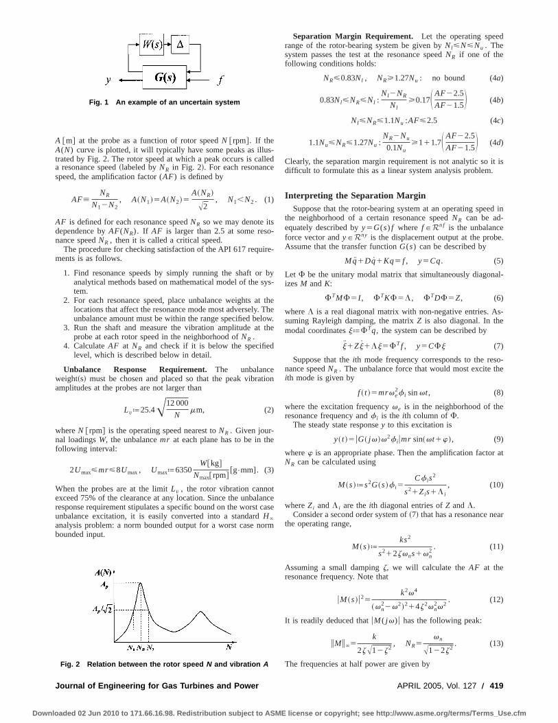
A @m# at the probe as a function of rotor speedN @rpm#. If theA(N) curve is plotted, it will typically have some peaks as illus-trated by Fig. 2. The rotor speed at which a peak occurs is calleda resonance speed~labeled byNR in Fig. 2!. For each resonancespeed, the amplification factor (AF) is defined by

AF[NR

N12N2, A~N1!5A~N2!5

A~NR!

A2, N1,N2 . (1)

AF is defined for each resonance speedNR so we may denote itsdependence byAF(NR). If AF is larger than 2.5 at some reso-nance speedNR , then it is called a critical speed.

The procedure for checking satisfaction of the API 617 require-ments is as follows.

1. Find resonance speeds by simply running the shaft or byanalytical methods based on mathematical model of the sys-tem.

2. For each resonance speed, place unbalance weights at thelocations that affect the resonance mode most adversely. Theunbalance amount must be within the range specified below.

3. Run the shaft and measure the vibration amplitude at theprobe at each rotor speed in the neighborhood ofNR .

4. CalculateAF at NR and check if it is below the specifiedlevel, which is described below in detail.

Unbalance Response Requirement.The unbalanceweight~s! must be chosen and placed so that the peak vibrationamplitudes at the probes are not larger than

Lvª25.4A12 000

Nmm, (2)

whereN @rpm# is the operating speed nearest toNR . Given jour-nal loadingsW, the unbalancemr at each plane has to be in thefollowing interval:

2Umax<mr<8Umax, Umaxª6350W@kg#

Nmax@rpm#@g•mm]. (3)

When the probes are at the limitLv , the rotor vibration cannotexceed 75% of the clearance at any location. Since the unbalanceresponse requirement stipulates a specific bound on the worst caseunbalance excitation, it is easily converted into a standardH`analysis problem: a norm bounded output for a worst case normbounded input.

Separation Margin Requirement. Let the operating speedrange of the rotor-bearing system be given byNl<N<Nu . Thesystem passes the test at the resonance speedNR if one of thefollowing conditions holds:

NR<0.83Nl , NR>1.27Nu : no bound (4a)

0.83Nl<NR<Nl :Nl2NR

Nl>0.17S AF22.5

AF21.5D (4b)

Nl<NR<1.1Nu :AF<2.5 (4c)

1.1Nu<NR<1.27Nu :NR2Nu

0.1Nu>111.7S AF22.5

AF21.5D (4d)

Clearly, the separation margin requirement is not analytic so it isdifficult to formulate this as a linear system analysis problem.

Interpreting the Separation MarginSuppose that the rotor-bearing system at an operating speed in

the neighborhood of a certain resonance speedNR can be ad-equately described byy5G(s) f where f PRn f is the unbalanceforce vector andyPRny is the displacement output at the probe.Assume that the transfer functionG(s) can be described by

Mq1Dq1Kq5 f , y5Cq. (5)

Let F be the unitary modal matrix that simultaneously diagonal-izesM andK:

FTMF5I , FTKF5L, FTDF5Z, (6)

whereL is a real diagonal matrix with non-negative entries. As-suming Rayleigh damping, the matrixZ is also diagonal. In themodal coordinatesjªFTq, the system can be described by

j1Zj1Lj5FTf , y5CFj (7)

Suppose that theith mode frequency corresponds to the reso-nance speedNR . The unbalance force that would most excite theith mode is given by

f ~ t !5mrve2f i sinvt, (8)

where the excitation frequencyve is in the neighborhood of theresonance frequency andf i is the ith column ofF.

The steady state responsey to this excitation is

y~ t !5uG~ j v!v2f i umr sin~vt1w!, (9)

wherew is an appropriate phase. Then the amplification factor atNR can be calculated using

M ~s!ªs2G~s!f i5Cf is

2

s21Zis1L i

, (10)

whereZi andL i are theith diagonal entries ofZ andL.Consider a second order system of~7! that has a resonance near

the operating range,

M ~s!ªks2

s212zvns1vn2

. (11)

Assuming a small dampingz, we will calculate theAF at theresonance frequency. Note that

uM ~s!u25k2v4

~vn22v2!214z2vn

2v2. (12)

It is readily deduced thatuM ( j v)u has the following peak:

iM i`5k

2zA12z2, NR5

vn

A122z2. (13)

The frequencies at half power are given by

Fig. 1 An example of an uncertain system

Fig. 2 Relation between the rotor speed N and vibration A



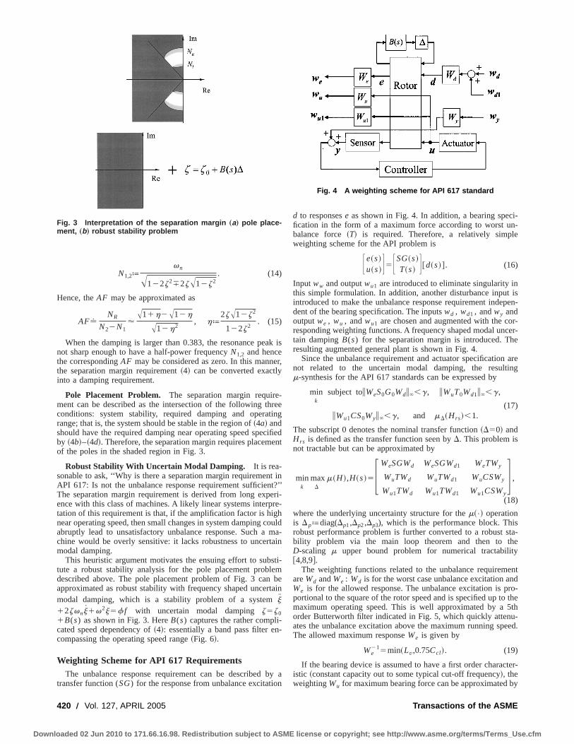
N1,2ªvn

A122z272zA12z2. (14)

Hence, theAF may be approximated as

AF8NR

N22N1'

A11h2A12h

A12h2, hª

2zA12z2

122z2. (15)

When the damping is larger than 0.383, the resonance peak isnot sharp enough to have a half-power frequencyN1,2 and hencethe correspondingAF may be considered as zero. In this manner,the separation margin requirement~4! can be converted exactlyinto a damping requirement.

Pole Placement Problem. The separation margin require-ment can be described as the intersection of the following threeconditions: system stability, required damping and operatingrange; that is, the system should be stable in the region of~4a! andshould have the required damping near operating speed specifiedby ~4b!–~4d!. Therefore, the separation margin requires placementof the poles in the shaded region in Fig. 3.

Robust Stability With Uncertain Modal Damping. It is rea-sonable to ask, ‘‘Why is there a separation margin requirement inAPI 617: Is not the unbalance response requirement sufficient?’’The separation margin requirement is derived from long experi-ence with this class of machines. A likely linear systems interpre-tation of this requirement is that, if the amplification factor is highnear operating speed, then small changes in system damping couldabruptly lead to unsatisfactory unbalance response. Such a ma-chine would be overly sensitive: it lacks robustness to uncertainmodal damping.

This heuristic argument motivates the ensuing effort to substi-tute a robust stability analysis for the pole placement problemdescribed above. The pole placement problem of Fig. 3 can beapproximated as robust stability with frequency shaped uncertainmodal damping, which is a stability problem of a systemj12zvnj1v2j5f f with uncertain modal dampingz5z01B(s) as shown in Fig. 3. HereB(s) captures the rather compli-cated speed dependency of~4!: essentially a band pass filter en-compassing the operating speed range~Fig. 6!.

Weighting Scheme for API 617 RequirementsThe unbalance response requirement can be described by a

transfer function (SG) for the response from unbalance excitation

d to responsese as shown in Fig. 4. In addition, a bearing speci-fication in the form of a maximum force according to worst un-balance force~T! is required. Therefore, a relatively simpleweighting scheme for the API problem is

Fe~s!

u~s!G5FSG~s!

T~s! G@d~s!#. (16)

Input ww and outputwu1 are introduced to eliminate singularity inthis simple formulation. In addition, another disturbance input isintroduced to make the unbalance response requirement indepen-dent of the bearing specification. The inputswd , wd1 , andwy andoutputwe , wu , andwu1 are chosen and augmented with the cor-responding weighting functions. A frequency shaped modal uncer-tain dampingB(s) for the separation margin is introduced. Theresulting augmented general plant is shown in Fig. 4.

Since the unbalance requirement and actuator specification arenot related to the uncertain modal damping, the resultingm-synthesis for the API 617 standards can be expressed by

mink

subject toiWeS0G0Wdi`,g, iWuT0Wd1i`,g,

(17)iWu1CS0Wyi`,g, and mD~Hrs!,1.

The subscript 0 denotes the nominal transfer function~D50! andHrs is defined as the transfer function seen byD. This problem isnot tractable but can be approximated by

mink

maxD

m~H !,H~s!5FWeSGWd WeSGWd1 WeTWy

WuTWd WuTWd1 WuCSWy

Wu1TWd Wu1TWd1 Wu1CSWy

G ,

(18)

where the underlying uncertainty structure for them~•! operationis Dpªdiag(Dp1,Dp2,Dp3), which is the performance block. Thisrobust performance problem is further converted to a robust sta-bility problem via the main loop theorem and then to theD-scaling m upper bound problem for numerical tractability@4,8,9#.

The weighting functions related to the unbalance requirementareWd andWe : Wd is for the worst case unbalance excitation andWe is for the allowed response. The unbalance excitation is pro-portional to the square of the rotor speed and is specified up to themaximum operating speed. This is well approximated by a 5thorder Butterworth filter indicated in Fig. 5, which quickly attenu-ates the unbalance excitation above the maximum running speed.The allowed maximum responseWe is given by

We215min~Lv,0.75Ccl!. (19)

If the bearing device is assumed to have a first order character-istic ~constant capacity out to some typical cut-off frequency!, theweightingWu for maximum bearing force can be approximated by

Fig. 3 Interpretation of the separation margin „a… pole place-ment, „b… robust stability problem

Fig. 4 A weighting scheme for API 617 standard



Wu5~s1vb!

Fmaxvb~«s11!, (20)

wherevb is the bandwidth of the bearing device. The factor« issimply chosen to be much smaller than 1/vb and much smallerthan 1/Nu . For a fluid film bearing,vb may be taken as infinite sothatWu becomes constant.Wu1 andWy are chosen as constants tohave a small effect on the synthesis at first. However, theseweighting functions will later play a significant role in reducingthe conservativeness by weighting the control effort.

The frequency shaping implied by~4! for B(s) can be approxi-mated using a 7th order elliptic filter whose gain outside of theseparation margin range is less than 0.001. The filter coefficientsare determined through a least square algorithm@10#. The normal-ized separation margin requirement and an example elliptic filterare shown in Fig. 6.

ExampleThe example system consists of a rotor, three sensors, and three

AMBs as shown in Fig. 7. For simplicity, it is assumed that the

three probe points and unbalance excitation locations for APIstandards are the same as the sensor and bearing locations.

The rotor has three actuator sleeves, three midspan unbalancedisks, and a coupling at the right end. The total mass is about 85kg and total length is about 2.7 m. The first four natural frequen-cies in RPM are 8600, 19,268, 37,997, and 60,648.

The operating range is selected to be 8,000–10,000 rpm so thatthe first bending natural frequency is within the operating range.The calculated vibration limit at probes is 0.028 mm and the worstcase unbalance is 14.4 g-mm from~2! and~3!. The AMB capaci-ties are assumed 6300 N up to the 265 Hz power signal band-width.

Results. To check if the API standards can be satisfied withthese bearings, a synthesis is performed with small constantweightings for the control effort. If a rotor is assessed~by ourmethod! to be infeasible for API standards, then we can be rea-sonably certain that there is no fluid film bearing which will meetAPI. On the other hand, if there is a controller, then there may bea bearing which also meets API, and it may be possible to ap-proximate the computed controller as stiffness and damping of abearing.

The peakm value is 0.1574 and the API standard can be satis-fied with the given actuator as shown in Fig. 8. The robust stabil-ity denotes the separation margin requirement, the nominal per-formance of the~1,1! diagonal block is for the unbalance responserequirement and the nominal performance of the~2,2! diagonalblock is for the actuator specification. The robust stability hasmost influence on the peakm value near the operating range.

Figure 9 shows the pole/zero maps of the augmented open-loopplant and closed-loop system. The seven poles along the requireddamping line for the separation margin in Fig. 9~a! are related tothe 7th order elliptic filter for the uncertain modal damping, whilethe three poles along the maximum operating range are related tothe 5th order Butterworth filter for the unbalance excitation. Inaddition, there is a lightly damped first bending mode~8600 rpm!near the imaginary axis, which is denoted by original pole. Thepole of the lightly damped first bending mode moves farther be-

Fig. 5 A weighting function for the worst case unbalanceexcitation

Fig. 6 7th order elliptic filter for the uncertain modal damping

Fig. 7 Example rotor model

Fig. 8 Results with the original actuator



yond the required damping line than is required to meet the sepa-ration margin requirement, which is denoted by moved pole asshown in Fig. 9~b!.

The maximum singular value of equivalent stiffness of the re-sulting control is shown in Fig. 10. The resulting controller doesnot exhibit the typical control shape of an AMB system, which isvery similar to a PD control. In order to test how much controleffort is required to meet the API standards, a simpler optimaldesign problem was solved. Here, the three bearings were as-sumed to be identical devices with fixed stiffness and damping.Thus, single values of stiffness and damping were found, whichsimultaneously satisfy 5.46•105 N/mm and 7.65•103 Nsec/mm,respectively. The equivalent stiffness at the bending natural fre-quency is 6.91•106 N/mm. The gain of the designed controller ismuch higher~the maximum value is 1.56•108 N/mm).

Although the API standards are satisfied, the designed control-ler is very conservative since all performance indices are muchless than 1.0~especially, the robust stability is 0.1283!, whichmeans that the control effort bound is unnecessarily high. In orderto reduce the conservativeness of the synthesis and to find aneconomic controller meeting the API requirements with minimumcontrol effort, the constant weighting for the control effort ischanged. The synthesis procedure is as follows: all weightings arethe same except for the control effort, whose initial values are themaximum force and vibration amplitude. Then, an optimalweighting constant is found to satisfy the API standard and theactuator specification through the bisection method. When the

maximum response is reduced by 11.4 times, the peakm value is1.8412 and robust stability is 0.9997. Both the API standards andthe actuator specification are satisfied as shown in Fig. 11.

The pole/zero map of the closed-loop system is shown in Fig.12. The moved pole is very close to the required damping line andthe conservativeness is reduced significantly.

The maximum singular value of the equivalent stiffness of thesecond controller is shown in Fig. 13. The controller has the de-sired shape to stabilize an AMB rotor system similar to a PDcontrol. The control effort is reduced significantly~particularly thegain at low frequencies! and the maximum equivalent stiffness is1.53•107 N/mm, which is a little bit higher than expected; how-ever, it is not unacceptably high considering non-collocation con-figuration and stabilization of an unstable AMB rotor system. Thatis, the m-analysis/synthesis is known to be conservative so itshould not be expected to be exactly same as the API standards.However, it can be said is that if the proposed sythesis is success-ful, then there is definitely a bearing to meet the API standards.

ConclusionThis paper discussed a possible control design problem for as-

sessing the feasibility of meeting the API 617 requirements with a

Fig. 9 Pole Õzero map: „a… augmented open-loop plant, „b…closed-loop system

Fig. 10 Stiffness of the designed controller

Fig. 11 Results after reducing the conservativeness



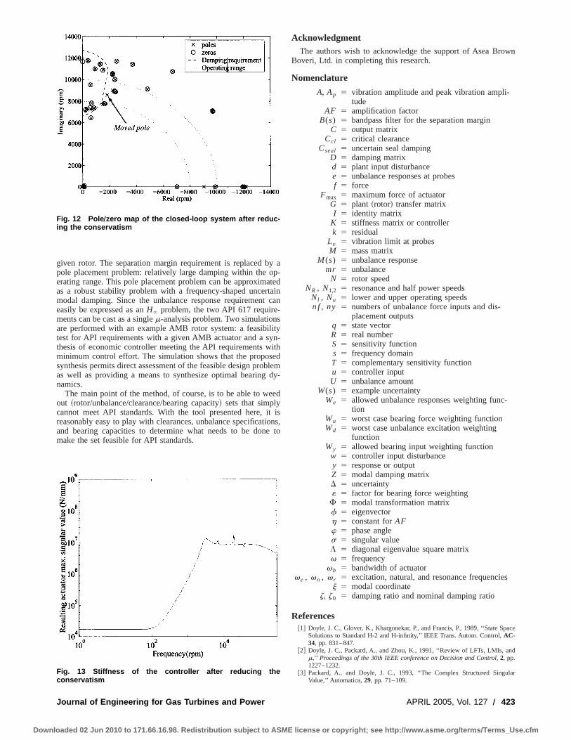
given rotor. The separation margin requirement is replaced by apole placement problem: relatively large damping within the op-erating range. This pole placement problem can be approximatedas a robust stability problem with a frequency-shaped uncertainmodal damping. Since the unbalance response requirement caneasily be expressed as anH` problem, the two API 617 require-ments can be cast as a singlem-analysis problem. Two simulationsare performed with an example AMB rotor system: a feasibilitytest for API requirements with a given AMB actuator and a syn-thesis of economic controller meeting the API requirements withminimum control effort. The simulation shows that the proposedsynthesis permits direct assessment of the feasible design problemas well as providing a means to synthesize optimal bearing dy-namics.

The main point of the method, of course, is to be able to weedout ~rotor/unbalance/clearance/bearing capacity! sets that simplycannot meet API standards. With the tool presented here, it isreasonably easy to play with clearances, unbalance specifications,and bearing capacities to determine what needs to be done tomake the set feasible for API standards.

AcknowledgmentThe authors wish to acknowledge the support of Asea Brown

Boveri, Ltd. in completing this research.

Nomenclature

A, Ap 5 vibration amplitude and peak vibration ampli-tude

AF 5 amplification factorB(s) 5 bandpass filter for the separation margin

C 5 output matrixCcl 5 critical clearance

Cseal 5 uncertain seal dampingD 5 damping matrixd 5 plant input disturbancee 5 unbalance responses at probesf 5 force

Fmax 5 maximum force of actuatorG 5 plant ~rotor! transfer matrixI 5 identity matrix

K 5 stiffness matrix or controllerk 5 residual

Lv 5 vibration limit at probesM 5 mass matrix

M (s) 5 unbalance responsemr 5 unbalance

N 5 rotor speedNR , N1,2 5 resonance and half power speeds

Nl , Nu 5 lower and upper operating speedsn f , ny 5 numbers of unbalance force inputs and dis-

placement outputsq 5 state vectorR 5 real numberS 5 sensitivity functions 5 frequency domainT 5 complementary sensitivity functionu 5 controller inputU 5 unbalance amount

W(s) 5 example uncertaintyWe 5 allowed unbalance responses weighting func-

tionWu 5 worst case bearing force weighting functionWd 5 worst case unbalance excitation weighting

functionWy 5 allowed bearing input weighting function

w 5 controller input disturbancey 5 response or outputZ 5 modal damping matrixD 5 uncertainty« 5 factor for bearing force weightingF 5 modal transformation matrixf 5 eigenvectorh 5 constant forAFw 5 phase angles 5 singular valueL 5 diagonal eigenvalue square matrixv 5 frequency

vb 5 bandwidth of actuatorve , vn , v r 5 excitation, natural, and resonance frequencies

j 5 modal coordinatez, z0 5 damping ratio and nominal damping ratio

References@1# Doyle, J. C., Glover, K., Khargonekar, P., and Francis, P., 1989, ‘‘State Space

Solutions to Standard H-2 and H-infinity,’’ IEEE Trans. Autom. Control,AC-34, pp. 831–847.

@2# Doyle, J. C., Packard, A., and Zhou, K., 1991, ‘‘Review of LFTs, LMIs, andm,’’ Proceedings of the 30th IEEE conference on Decision and Control, 2, pp.1227–1232.

@3# Packard, A., and Doyle, J. C., 1993, ‘‘The Complex Structured SingularValue,’’ Automatica,29, pp. 71–109.

Fig. 12 Pole Õzero map of the closed-loop system after reduc-ing the conservatism

Fig. 13 Stiffness of the controller after reducing theconservatism



@4# Zhou, K., Doyle, J. C., and Glover, K., 1996,Robust and Optimal Control,Prentice-Hall, Englewood Cliffs, NJ.

@5# Cloud, C. H., Foiles, W. C., Li, G., Maslen, E. H., and Barrett, L. E., 2002,‘‘Practical Applications of Singular Value Decomposition in Rotordynamics,’’in Proceedings of 6th International Conference on Rotor Dynamics.

@6# Zames, G., 1966, ‘‘On the Input-Output Stability of Nonolinear Time-VaryingFeedback Systems, Part I,’’ IEEE Trans. Autom. Control,11, pp. 228–238.

@7# API 617, Axial and Centrifugal Compressors and Turboexpanders for Petro-

leum, Chemical and Gas Industry Services, American Petroleum Institute,Washinton D.C., 2002.

@8# Balas, G. J., Doyle, J. C., Glover, K., Packard, A. K., and Smith, R., 1995,mAnalysis and Synthesis Toolbox User’s Guide, The MathWorks, Natick, MA.

@9# Skogestad, S., and Postlethwaite, I., 1996,Multivariable Feedback Control:Analysis and Design, Wiley, West Sussex, England.

@10# Branch, M. A., and Grace, A., 1996,MATLAB Optimization Toolbox User’sGuide, The MathWorks, Natick, MA.



Itzhak GreenGeorgia Institute of Technology,

GWW School of Mechanical Engineering,Atlanta, GA 30332

Fellow ASME

Cody CaseySchlumberger,

14910 Airline Road,Rosharon, TX 77583

Crack Detection in a RotorDynamic System by VibrationMonitoring—Part I: AnalysisMany practical rotor dynamic systems contain shaft/rotor elements that are highly sus-ceptible to transverse cross-sectional cracks due to fatigue. The early detection of me-chanical malfunction that can be provided by an effective vibration monitoring system isessential. Two theoretical analyses, global and local asymmetry crack models, are utilizedto identify characteristics of the system response that may be directly attributed to thepresence of a transverse crack in a rotating shaft. A model consisting of an overhungwhirling rotor is utilized to match an experimental test rig. A 2X harmonic component ofthe system response is shown to be the primary response characteristic resulting from theintroduction of a crack. Once the unique characteristics of the system response are iden-tified, they serve then as target observations for the monitoring system.@DOI: 10.1115/1.1789514#

1 IntroductionAs rotating machinery is designed to operate at higher mechani-

cal efficiency; operating speed, power, and load are increased asweight and dimensional tolerances are decreased. The result is asignificantly increased level of operating stress in modern rotatingmachinery. As a consequence, many practical rotordynamic sys-tems contain shaft/rotor elements that are highly susceptible totransverse cross-sectional cracks due to fatigue. To accurately pre-dict the response of a system to the presence of a transverse crack,an appropriate crack model is essential. Once the crack is includedin the system model, unique characteristics of the system responsecan be identified and attributed directly to the presence of thecrack. These predicted indicators then serve as target observationsfor monitoring systems.

A significant amount of research involving the prediction of theresponse of shaft/rotor systems to the presence of a transversecrack, and the detection of transverse cracks in rotating shafts byvibration monitoring, has been completed in the last 30 to 40years. This work is an extension of a body of research focused ona flexibly mounted rotor~FMR! mechanical face seal system@1#.The dynamics of the FMR mechanical face seal system have beenextensively investigated@2–5#. In Ref. @2# the coupled dynamicsof the seal and shaft is investigated including effects of shaftinertia and slenderness, fluid film, secondary seal, flexiblymounted rotating element, and an axial offset of the rotor center ofmass. The steady-state response was investigated by implement-ing a complex extended transfer-matrix method. In Ref.@3# anexperimental correlation is investigated between the presence ofhigher harmonic oscillations in the test rig system and seal facecontact. The dynamics behavior of the FMR seal itself was inves-tigated in Refs.@4# and@5#. Seal failure, diagnostics, control, andeventual performance restoration are extensively discussed inRefs. @6–10#. To achieve these goals it is imperative that failurecharacteristics of seal and shaft are well differentiated. The influ-ence of a crack in a seal-driving shaft is the concern of this work.

An uncracked shaft has constant stiffness, and thus constantdisplacement under a fixed load, regardless of the angle of rota-tion. In a cracked shaft, the cracked portion of the cross section is

not capable of supporting a tensile stress. Therefore the displace-ment, as a function of the stiffness, is minimum when the crack isclosed and maximum when the crack is open. This opening andclosing behavior, which is referred to as ‘‘breathing,’’ results intime-dependent stiffness coefficients in the equations of motion ofthe system, which is difficult to work with. Obtaining solutionsusually requires making broad simplifying assumptions or sometype of numerical approximation.

Systems in which static displacements and vibrational ampli-tudes remain very small result in a crack that remains essentiallyopen regardless of the angle of rotation. This type of crack, whichis essentially a local stiffness asymmetry, is referred to as a ‘‘gap-ing’’ crack. The analysis of systems containing a gaping crack isextremely useful since the response characteristics, or crack indi-cators, identified in the gaping crack analysis are also present inthe analysis of systems containing a breathing crack. Furthermore,these indicators prove to be the most practical, in terms of imple-mentation, in the detection of real cracks. Also, since the intro-duction of a crack into a rotating system, on the most basic level,results in a system with a stiffness asymmetry, the analysis ofsystems containing an asymmetry is fundamental to the study ofthe dynamics of cracked rotating systems.

The primary effect of the presence of a crack in a rotating shaftis clearly a local reduction in stiffness. This highly localized effectdoes not influence the stiffness of the regions of the rotor awayfrom the cracked cross section. Regardless of the type of crackmodel used for analysis, the effective overall stiffness of the rotoris no longer symmetric. The analysis of the response of a rotorwith designed-in asymmetry is therefore part of the fundamentalbasis for the analysis of the dynamics of shafts containing a trans-verse crack.

A free response of a two degree-of-freedom rotor with asym-metric moments of inertia@11# shows a range of shaft speeds inwhich the response is unstable. The appearance of a region ofinstability near the first natural frequency is confirmed in Ref.@12#, as well as the 2X harmonic response in an analysis of alinearly asymmetric shaft. In Ref.@13# the 2X resonance is alsopredicted at approximately one-half of the first natural frequency.An intuitive explanation for the existence of a region of instabilityand a 2X harmonic response in shafts with dissimilar moments ofinertia is given in Ref.@14#. It is important to note that for rotatingsystems, the terms ‘‘natural frequency’’ and ‘‘whirl frequency’’ aresynonymous. Also, the term ‘‘critical speed’’ refers to a shaftspeed for which one or more of the natural~whirl! frequencies of




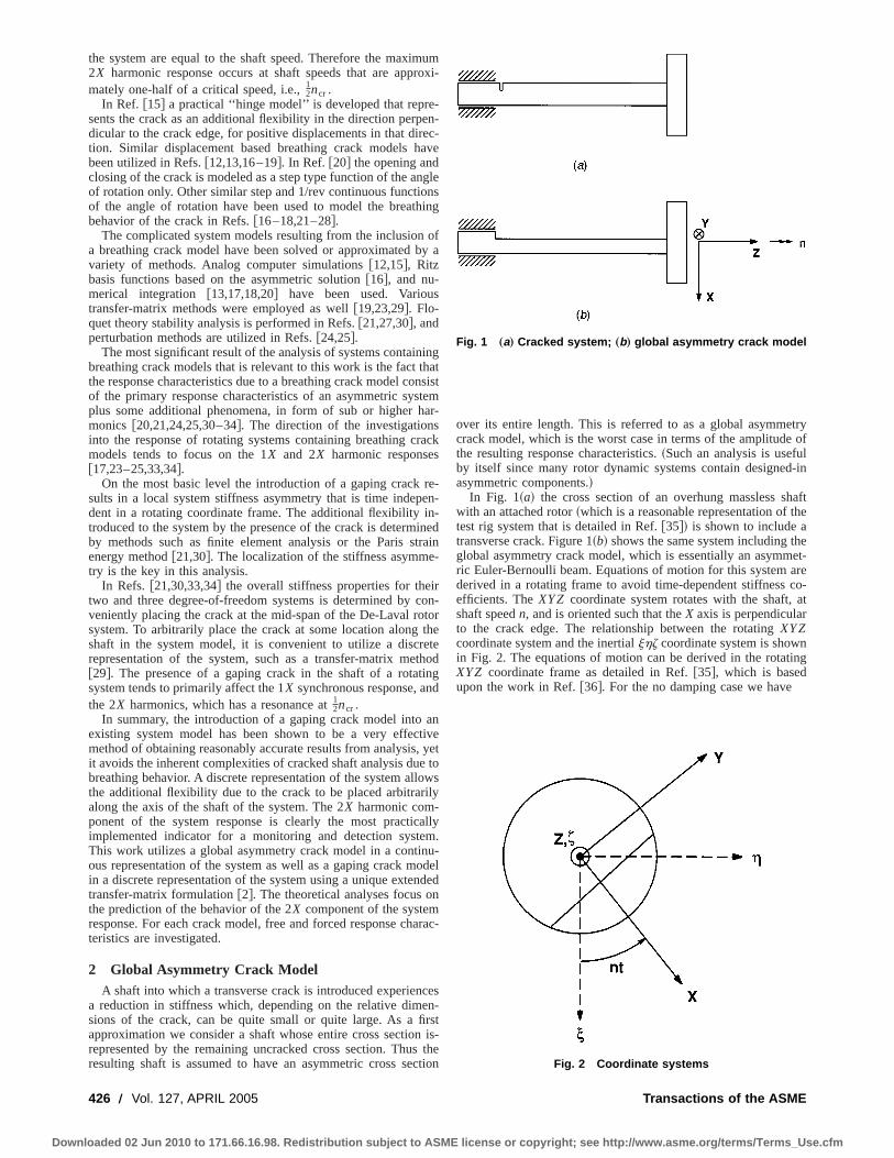
the system are equal to the shaft speed. Therefore the maximum2X harmonic response occurs at shaft speeds that are approxi-mately one-half of a critical speed, i.e.,1

2ncr .In Ref. @15# a practical ‘‘hinge model’’ is developed that repre-

sents the crack as an additional flexibility in the direction perpen-dicular to the crack edge, for positive displacements in that direc-tion. Similar displacement based breathing crack models havebeen utilized in Refs.@12,13,16–19#. In Ref. @20# the opening andclosing of the crack is modeled as a step type function of the angleof rotation only. Other similar step and 1/rev continuous functionsof the angle of rotation have been used to model the breathingbehavior of the crack in Refs.@16–18,21–28#.

The complicated system models resulting from the inclusion ofa breathing crack model have been solved or approximated by avariety of methods. Analog computer simulations@12,15#, Ritzbasis functions based on the asymmetric solution@16#, and nu-merical integration @13,17,18,20# have been used. Varioustransfer-matrix methods were employed as well@19,23,29#. Flo-quet theory stability analysis is performed in Refs.@21,27,30#, andperturbation methods are utilized in Refs.@24,25#.

The most significant result of the analysis of systems containingbreathing crack models that is relevant to this work is the fact thatthe response characteristics due to a breathing crack model consistof the primary response characteristics of an asymmetric systemplus some additional phenomena, in form of sub or higher har-monics @20,21,24,25,30–34#. The direction of the investigationsinto the response of rotating systems containing breathing crackmodels tends to focus on the 1X and 2X harmonic responses@17,23–25,33,34#.

On the most basic level the introduction of a gaping crack re-sults in a local system stiffness asymmetry that is time indepen-dent in a rotating coordinate frame. The additional flexibility in-troduced to the system by the presence of the crack is determinedby methods such as finite element analysis or the Paris strainenergy method@21,30#. The localization of the stiffness asymme-try is the key in this analysis.

In Refs. @21,30,33,34# the overall stiffness properties for theirtwo and three degree-of-freedom systems is determined by con-veniently placing the crack at the mid-span of the De-Laval rotorsystem. To arbitrarily place the crack at some location along theshaft in the system model, it is convenient to utilize a discreterepresentation of the system, such as a transfer-matrix method@29#. The presence of a gaping crack in the shaft of a rotatingsystem tends to primarily affect the 1X synchronous response, andthe 2X harmonics, which has a resonance at1

2ncr .In summary, the introduction of a gaping crack model into an

existing system model has been shown to be a very effectivemethod of obtaining reasonably accurate results from analysis, yetit avoids the inherent complexities of cracked shaft analysis due tobreathing behavior. A discrete representation of the system allowsthe additional flexibility due to the crack to be placed arbitrarilyalong the axis of the shaft of the system. The 2X harmonic com-ponent of the system response is clearly the most practicallyimplemented indicator for a monitoring and detection system.This work utilizes a global asymmetry crack model in a continu-ous representation of the system as well as a gaping crack modelin a discrete representation of the system using a unique extendedtransfer-matrix formulation@2#. The theoretical analyses focus onthe prediction of the behavior of the 2X component of the systemresponse. For each crack model, free and forced response charac-teristics are investigated.

2 Global Asymmetry Crack ModelA shaft into which a transverse crack is introduced experiences

a reduction in stiffness which, depending on the relative dimen-sions of the crack, can be quite small or quite large. As a firstapproximation we consider a shaft whose entire cross section is-represented by the remaining uncracked cross section. Thus theresulting shaft is assumed to have an asymmetric cross section

over its entire length. This is referred to as a global asymmetrycrack model, which is the worst case in terms of the amplitude ofthe resulting response characteristics.~Such an analysis is usefulby itself since many rotor dynamic systems contain designed-inasymmetric components.!

In Fig. 1~a! the cross section of an overhung massless shaftwith an attached rotor~which is a reasonable representation of thetest rig system that is detailed in Ref.@35#! is shown to include atransverse crack. Figure 1~b! shows the same system including theglobal asymmetry crack model, which is essentially an asymmet-ric Euler-Bernoulli beam. Equations of motion for this system arederived in a rotating frame to avoid time-dependent stiffness co-efficients. TheXYZ coordinate system rotates with the shaft, atshaft speedn, and is oriented such that theX axis is perpendicularto the crack edge. The relationship between the rotatingXYZcoordinate system and the inertialjhz coordinate system is shownin Fig. 2. The equations of motion can be derived in the rotatingXYZ coordinate frame as detailed in Ref.@35#, which is basedupon the work in Ref.@36#. For the no damping case we have

Fig. 1 „a… Cracked system; „b… global asymmetry crack model

Fig. 2 Coordinate systems



Fm 0 0 0

0 m 0 0

0 0 I t 0

0 0 0 I t

G H X

YgX

gY

J 1F 0 22mn 0 0

2mn 0 0 0

0 0 0 n~ I P22I t!

0 0 2n~ I P22I t! 0

G H X

YgX

gY

J1F k11Y2mn2 0 0 2k12Y

0 k11X2mn2 k12X 0

0 k12X n2~ I P2I t!1k22X 0

2k12Y 0 0 n2~ I P2I t!1k22Y

G H XYgX

gY

J 5$F%, (1)

whereX, Y, gX , andgY are displacements and tilts about theXandY axes, respectively,m is the mass or the rotor,n is the shaftspeed,I p andI t are the polar and transverse moments of inertia ofthe rotor, andki j are stiffness elements, which are determined inthe Appendix. Since in the tested system the mass of the shaft issignificantly less than the mass of the rotor, it is neglected. Theeffects of internal energy dissipation in the free response analysisare negligible. Therefore internal damping will be incorporatedinto the equations of motion for the forthcoming forced responseanalysis. Equation~1! forms a system of coupled linear ordinarydifferential equations including gyroscopic effects, where$F% is avector of generalized applied forces.

2.1 Undamped Free Response.The goal of the free re-sponse analysis is to obtain the system eigenvalues, which are thenatural, or whirl, frequencies. The homogeneous form of the ma-trix equation of motion given in Eq.~1! has the general form

@M #$S%1@C#$S%1@K#$S%5$0%, (2)

where@M#, @C#, and@K# are inertia, ‘‘damping’’~i.e., Coriolis andgyroscopic effects!, and stiffness matrices, and$S% is the general-ized vector of displacements. The system is conveniently ex-pressed in a state-variable form by defining the following@A# and@B# matrices:

@A#5F2@K# @0#

@0# @M #G ; @B#5F @0# 2@K#

2@K# 2@C#G . (3)

The system expressed in state-variable form is then given by

$ S%5@A#21@B#$S%, (4)

where $S% is the state vector of the displacements and tilts andtheir first derivatives, which is given by

$S%5$X Y gX gY X Y gX gY%T. (5)

For this state vector form the state matrix is formed by@A#21@B#.The eigenvalues and eigenvectors, or whirl frequencies and

mode shapes, are then obtained, corresponding to the state vectorexpressed in the rotatingXYZ frame. For monitoring purposes theabsolute whirl frequencies are of interest since the monitoringsystem is typically fixed in the inertialjhz coordinate frame. Theabsolute whirl frequencies,v, i.e., the eigenvalues expressed inthe inertialjhz frame, can be obtained from

v5v01n, (6)

wherev0 is the relative whirl frequency, andn is the shaft speed.Since the state matrix,@A#21@B#, is 838, four conjugate pairs ofeigenvalues are obtained. The eigenvalues are purely imaginarysince damping or dissipation effects are neglected in this freeresponse analysis.

In rotordynamics, the sign of the frequency is meaningful dueto the fact that shaft whirl can occur with a negative sense, op-posing the direction of shaft rotation, or a positive sense, in thedirection of shaft rotation. The proper sign can be assigned to the

magnitude of each eigenvalue pair which yields forward or back-ward whirl according to the analysis detailed in Ref.@35#. Therelative whirl frequencies resulting from the analysis,v0 , are as-signed the appropriate direction and the absolute whirl frequenciesv are obtained from Eq.~6!. Figures 3 show the whirl frequenciesas a function of shaft speed for simulated crack depths rangingfrom 0–40% of the shaft diameter. The ‘‘3’’ symbols along thehorizontal axis of Fig. 3 indicate shaft speeds for which one ormore of the eigenvalues has a positive real part, i.e., shaft speedsfor which the response is unstable. This instability is solely due toan asymmetric cross section of a purely elastic shaft~recall thatinternal damping has been neglected in this section! ~see alsoRefs.@11,12,14#!. Two reference lines are also plotted in each ofthe figures. The intersection of thev5n line with the locus ofwhirl frequencies indicates shaft speeds which are equivalent to awhirl frequency, i.e., primary (1X) critical speeds. The intersec-tion of the v52n line with the locus of whirl frequencies indi-cates shaft speeds which are one-half of a whirl frequency, i.e.,secondary (2X) critical speeds.

When operating at a secondary critical speed, the 2X compo-nent of the response of the system is occurring at a natural fre-quency of the system, and will therefore exhibit a resonance be-havior. It is at these 2X critical speeds that the 2X response isexpected to be maximum. Comparing the predicted shaft speeds atwhich the 2X resonance occurs for various crack depths clearlyshows a decrease in the natural frequencies of the system due tothe presence of the crack. This change in the system natural fre-quency is due to the reduction in system stiffness resulting fromthe crack. The predicted 2X resonance shaft speeds for the globalasymmetry crack model are given in Table 1.

2.2 Damped Forced Response.The gravity forced re-sponse of the system model containing the global asymmetrycrack model is fundamentally important when considering crackdetection. The resulting 2X harmonic response is the most reliableand widely used indicator of crack existence.

Energy dissipation effects are included in this analysis in orderto observe the influence of the introduction and propogation of thesimulated crack on the magnitude of the system response at 2Xresonance shaft speeds. The equivalent viscous damping coeffi-cients are incorporated into the matrix equation of motion by de-fining a new damping matrix,@C#, according to

@C#5@C#1@D#, (7)

where @C# is the matrix which contains the Coriolis and gyro-scopic effects, and the@D# matrix contains the equivalent viscousdamping coefficients. The damping matrix@D# is given by

@D#5F d11Y0 0 2d12Y

0 d11Xd12X

0

0 d12Xd22X

0

2d12Y0 0 d22Y

G , (8)



where di j X5di j Y

5ceqi j5

12b (ki j X

1ki j Y)/v. Here average stiff-

ness elements are used so thatdi j Xanddi j Y

are equal. It is neces-sary to construct the complex equations of motion in the followinganalysis. The equation of motion, including internal damping, hasthe form

@M #$S%1@C#$S%1@K#$S%5$F%. (9)

The equations of motion are derived in the shaft-fixedXYZcoordinate frame. The direction along which gravity acts, which isa stationary vector along thej axis of the inertialjhz coordinate

frame, can be represented by a vector that is rotating with a nega-tive sense in theXYZ frame. Therefore the forcing function re-sulting from gravity has the form

Fg5mge2 int, (10)

wherem is the mass of the rotor,g is the gravitational accelerationandn is the shaft speed. The vector of forces that is now includedin the right-hand side of the equations of motion@Eq. ~1!# is thengiven, in the rotatingXYZ coordinate frame, by

$F%5H mgcos~nt!2mgsin~nt!

00

J . (11)

The equations of motion are then combined by defining the fol-lowing complex variables for the displacementr and tilt f:

r5X1 iY, (12)

f5gX1 igY . (13)

The resulting complex equations of motion are

Fig. 3 Global asymmetry model free response at various crack depth values: „a… uncracked; „b… 20%; „c… 30%; „d… 40%

Table 1 2 X resonance shaft speeds—global asymmetry modelfree response

% cracked Shaft speed~Hz!

0 70.6210 67.0420 60.5530 52.2940 43.01



r1D11r1~vr22n2!r2S Dkr

krvr

2D r* 1~2n!i r1D12mf

1~vrfm

2 !if1S Dkrf

krfvrfm

2 D if* 5ge2 int, (14)

f1D22f1Fn2S I p

I t21D1vf

2 Gf1S Dkf

kfvf

2 Df* 2FnS I p

I t22D G i f

2D12I ti r2~vrf I t

2 !ir1S Dkrf

krfvrf I t

2 D ir* 50, (15)

where the ‘‘* ’’ denotes the complex conjugate of the variables inEqs.~12! and ~13!, and

vr5kr

m, vf5

kf

I t, vrfm

5krf

m, vrf I t

5krf

I t,

kr512 ~k11X

1k11Y!,

kf512 ~k22X

1k22Y!, krf5

12 ~k12X

1k12Y!, Dkr5kr2k11Y

,

Dkf5kf2k22Y, Dkrf5krf2k12Y

, D115d11X

m5

d11Y

m,

D12m5

d12X

m5

d12Y

m, D12I t

5d12X

I t5

d12Y

I t,

D225d22X

I t5

d22Y

I t.

To solve this system of equations, solutions of the followingforms are chosen for the displacementr, and tilt f:

r5Aeint1Be2 int, (16)

f5Ceint1De2 int, (17)

whereA, B, C, andD are arbitrary complex numbers. These so-lutions are substituted into Eqs.~14! and ~15! and the complexcoefficientsA, B, C, and D are determined. Recalling that thedisplacement and tilt in the rotatingXYZ coordinate frame aregiven by Eqs.~16! and ~17!, the displacementu and tilt g in theinertial coordinate frame are obtained according to

u5reint, (18)

g5feint. (19)

The displacement and tilt expressed in the inertial coordinateframe are of interest since the experimental data provided by themonitoring system is also obtained in the inertial coordinate frame~according to Ref.@35#!. From Eqs.~16!–~19! it is clear that thedisplacement and tilt in the inertial coordinate frame will have theform

u5Aei2nt1B, (20)

g5Cei2nt1D. (21)

The presence of the 2X harmonic is evident in Eqs.~20! and~21!.The magnitudes of coefficientsA andC are the magnitudes of the2X harmonic response, in the inertial frame, of the displacementand tilt, respectively. Equations~20! and~21! predict displacementand tilt responses which have circular shapes, having radii ofuAu,anduCu, and are offset byB andD. It is important to note that dueto the form of the assumed solutions@Eqs. ~16! and ~17!#, theresulting solutions@Eqs. ~20! and ~21!# are limited to predictingonly circular orbit shapes of the 2X component.

Figures 4 show the predicted magnitude of the 2X tilt response,based on the global asymmetry crack model, as a function of shaftspeed, for two speed ranges, and crack depths varying from 0 to40% of the shaft diameter. The magnitudes plotted show the radii

of the predicted circular 2X tilt responses. It is clear that for anarbitrary shaft speed, the amplitude of the 2X response is pre-dicted to increase as the crack depth increases.

The magnitudes of the 2X component of the response plotted inFig. 4~a! are significantly smaller than those plotted in Fig. 4~b!.The range of shaft speeds shown in Fig. 4~b! contains 2X resonantspeeds for each crack depth.

As predicted, the 2X resonant speeds decrease as the crackdepth increases. The 2X resonance shaft speeds predicted basedon this global asymmetry crack model forced response analysisare given in Table 2. These predicted 2X resonance shaft speedsagree with the 2X resonance shaft speeds predicted in the globalasymmetry model free response analysis, which are given in Table1. Since the 0% simulated crack depth results in a system withsymmetric stiffness properties, no 2X resonance is predicted forthe forced response analysis. Damping is light, thus numericallyTables 1 and 2 provide similar 2X results.

3 Local Asymmetry Crack ModelPerhaps the most important effect of the presence of a trans-

verse crack in a rotating shaft is the highly localized flexibility

Fig. 4 Global asymmetry model forced tilt 2 X response: „a…Low-speed range; „b… high-speed range



that is introduced. To locally represent the stiffness properties of acracked cross section in an otherwise uncracked shaft, it is neces-sary to determine the additional flexibility due to the presence ofthe crack, and incorporate this flexibility into a discrete represen-tation of the system. In this study a transfer-matrix method wasemployed to accomplish this desired localizing effect. Figure 5shows the cracked system represented by three lumped stiffnesselements;@F1#, @Fcrack#, and @F2#, and one lumped inertia ele-ment@P#. Since the mass of the shaft is significantly less than themass of the rotor, the mass of the shaft is neglected.

The purpose of this section is to present the analytical portionof the analysis of the cracked system including a local asymmetrycrack model using the complex extended transfer-matrix method@2,37# for free and forced response analyses, along with relevantresults. As previously, damping effects will be incorporated intothe forced response analysis.

3.1 Crack Flexibility. The localized additional flexibilitycan be represented by a lumped parameter element. A section of ashaft containing a crack of deptha is shown, under general load-ing, in Fig. 6~a!. Figure 6~b! shows the cross section of the shaftsection in Fig. 6~a! at the location of the transverse crack. Thegeneralized displacementui in the i direction is obtained by uti-lizing Castigliano’s theorem@21,30#:

ui5]

]PiE

0

a

J~Y!dY, (22)

wherePi is the generalized force associated withui , andJ(Y),according to Tada, Paris, and Irwin@37#, is the strain energy den-sity function given by

J~a!512n2

E F S (i 51

6

KIi D 2

1S (i 51

6

KIIi D 2

1~11n!S (i 51

6

KIIIi D 2G , (23)

wheren is Poisson’s ratio,E is Young’s Modulus, andKni is thecrack stress intensity factor for moden due to Pi . The stressintensity factors for a unit width strip containing a crack of deptha are evaluated according to

Kni5s iApaFnS a

h D , (24)

wheres i are the stresses due to the loadPi at the crack,Fn(a/h)are appropriate intensity functions, andh is the total strip length~see Fig. 6~b!!.

The additional flexibility due to the crack for a unit width stripcan be written as

ci j 5]2

]Pi]PjE

0

a

J~Y!dY (25)

which, after integration along the crack edge, becomes

ci j 5]2

]Pi]PjE

2b

b E0

a

J~Y!dY. (26)

The current analysis is not concerned with torsion or axial dis-placement, hence onlyc22, c33, c44, c45, c54, and c55 are re-quired. These elements are then given byFig. 5 Local asymmetry crack model

Fig. 6 Local crack model: „a… shaft section containing a crack;„b… crack cross section

Table 2 2 X resonance shaft speeds—global asymmetry modelforced response


010 67.0420 60.5530 52.2940 43.01



c2254~12n2!

pER E0

bE0

a

YFII2 S Y

hD dYdX, (27)

c3354~12n2!

pER E0

bE0

a

YFII2 S Y

hD dYdX, (28)

c44532~12n2!

pER3 E0

bE0

a

X2YFIY2 S Y

hD dYdX, (29)

c455c55564~12n2!

pER3 E0

bE0

a

XYA12X2FIXS Y

hDFIYS Y

hD dYdX,

(30)

c55564~12n2!

pER3 E0

bE0

a

~12X2!YFIX2 S Y

hD dYdX, (31)

where b5b/R, X5X/R, Y5Y/R, a5a/R, and h5h/R. Thecorresponding intensity functions are given by

FIXS a

h D5F tan~bc!

bcG1/2

@ .9321.199~12sin~bc!!4#/cos~bc!,

(32)

FIYS a

h D5F tan~bc!

bcG1/2F .7521.202S a

h D1.37~12sin~bc!!3GY cos~bc!, (33)

FII S a

h D5F1.1222.561S a

h D1.085S a

h D 2

1.18S a

h D 3GY S 12a

h D 1/2

, (34)

FIII S a

h D5F tan~bc!

bcG1/2

, (35)

bc5S pa

2h D . (36)

The additional flexibilities due to the presence of the crack maytherefore be obtained by numerically integrating Eqs.~27!–~31!.Dimensionless flexibilities can be obtained according to

c225c22

pER

~12n2!, c335c33

pER

~12n2!,

c445c44

pER3

~12n2!c455c45

pER3

~12n2!, (37)

c555c55

pER3

~12n2!,

where the overbar indicates the nondimensional value. These di-mensionless flexibilities are plotted in Fig. 7, for crack depths upto 50% of the shaft diameter. These local flexibilities may now beintroduced appropriately into the discrete representation of thesystem.

3.2 Transfer Matrix. The transfer-matrix method is alumped parameter method in which inertial properties of the sys-tem are lumped into point matrices, and stiffness properties of thesystem are represented by lumped field matrices@2#; both relatestate vectors at the two ends of a shaft element. The state vector atstation i, expressed in the rotatingXYZ coordinate frame, is de-fined as

$Z% i5$uX uY MY 2VX 2uY uX MX VY%T, (38)

whereu, u, M, andV are the complex magnitudes of the displace-ment, tilt, moment, and shear force, respectively.

The Field Matrix. The state vector at the left of stationi,$Z% i

L , is related to the state vector at the right of stationi 21,$Z% i 21

R , by the field matrix@Fi #:

$Z% iL5@Fi #$Z% i 21

R . (39)

The field matrix@Fi # has the form

@Fi #5

l

1 l il i2

2EI

l i3

6EI0 0 0 0

0 1l i

EI

l i2

2EI0 0 0 0

0 0 1 l i 0 0 0 0

0 0 0 1 0 0 0 0

0 0 0 0 1 l il i2

2EI

l i3

6EI

0 0 0 0 0 1l i

EI

l i2

2EI

0 0 0 0 0 0 1 l i

0 0 0 0 0 0 0 1

m, (40)

wherel i is the length of the field,E is Young’s modulus, andI isthe area moment of inertia of the field cross section.

The Crack Matrix. The crack is represented by a field matrixwhich contains the additional flexibilities introduced by the pres-ence of the crack. The crack field matrix@Fcrack# has the form

Fig. 7 Dimensionless crack flexibilities



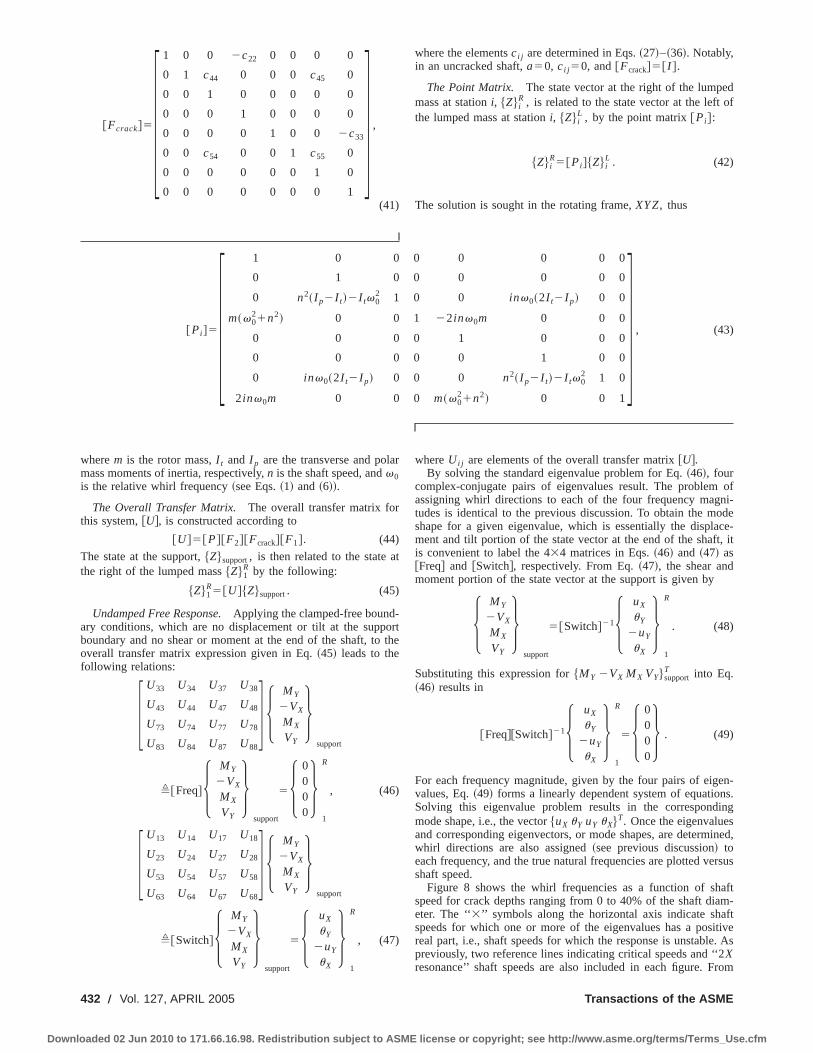
@Fcrack#531 0 0 2c22 0 0 0 0

0 1 c44 0 0 0 c45 0

0 0 1 0 0 0 0 0

0 0 0 1 0 0 0 0

0 0 0 0 1 0 0 2c33

0 0 c54 0 0 1 c55 0

0 0 0 0 0 0 1 0

0 0 0 0 0 0 0 1

4 ,

(41)

where the elementsci j are determined in Eqs.~27!–~36!. Notably,in an uncracked shaft,a50, ci j 50, and@Fcrack#5@ I #.

The Point Matrix. The state vector at the right of the lumpedmass at stationi, $Z% i

R , is related to the state vector at the left ofthe lumped mass at stationi, $Z% i

L , by the point matrix@Pi #:

$Z% iR5@Pi #$Z% i

L . (42)

The solution is sought in the rotating frame,XYZ, thus

@Pi #531 0 0 0 0 0 0 0

0 1 0 0 0 0 0 0

0 n2~ I p2I t!2I tv02 1 0 0 inv0~2I t2I p! 0 0

m~v021n2! 0 0 1 22inv0m 0 0 0

0 0 0 0 1 0 0 0

0 0 0 0 0 1 0 0

0 inv0~2I t2I p! 0 0 0 n2~ I p2I t!2I tv02 1 0

2inv0m 0 0 0 m~v021n2! 0 0 1

4 , (43)

wherem is the rotor mass,I t and I p are the transverse and polarmass moments of inertia, respectively,n is the shaft speed, andv0is the relative whirl frequency~see Eqs.~1! and ~6!!.

The Overall Transfer Matrix. The overall transfer matrix forthis system,@U#, is constructed according to

@U#5@P#@F2#@Fcrack#@F1#. (44)

The state at the support,$Z%support, is then related to the state atthe right of the lumped mass$Z%1

R by the following:

$Z%1R5@U#$Z%support. (45)

Undamped Free Response.Applying the clamped-free bound-ary conditions, which are no displacement or tilt at the supportboundary and no shear or moment at the end of the shaft, to theoverall transfer matrix expression given in Eq.~45! leads to thefollowing relations:

FU33 U34 U37 U38

U43 U44 U47 U48

U73 U74 U77 U78

U83 U84 U87 U88

G H MY

2VX

MX

VY

Jsupport

,@Freq#H MY

2VX

MX

VY

Jsupport

5H 0000J

1

R

, (46)

FU13 U14 U17 U18

U23 U24 U27 U28

U53 U54 U57 U58

U63 U64 U67 U68

G H MY

2VX

MX

VY

Jsupport

,@Switch#H MY

2VX

MX

VY

Jsupport

5H uX

uY

2uY

uX

J1

R

, (47)

whereUi j are elements of the overall transfer matrix@U#.By solving the standard eigenvalue problem for Eq.~46!, four

complex-conjugate pairs of eigenvalues result. The problem ofassigning whirl directions to each of the four frequency magni-tudes is identical to the previous discussion. To obtain the modeshape for a given eigenvalue, which is essentially the displace-ment and tilt portion of the state vector at the end of the shaft, itis convenient to label the 434 matrices in Eqs.~46! and ~47! as@Freq# and @Switch#, respectively. From Eq.~47!, the shear andmoment portion of the state vector at the support is given by

H MY

2VX

MX

VY

Jsupport

5@Switch#21H uX

uY

2uY

uX

J1

R

. (48)

Substituting this expression for$MY 2VX MX VY%supportT into Eq.

~46! results in

@Freq#@Switch#21H uX

uY

2uY

uX

J1

R

5H 0000J . (49)

For each frequency magnitude, given by the four pairs of eigen-values, Eq.~49! forms a linearly dependent system of equations.Solving this eigenvalue problem results in the correspondingmode shape, i.e., the vector$uX uY uY uX%T. Once the eigenvaluesand corresponding eigenvectors, or mode shapes, are determined,whirl directions are also assigned~see previous discussion! toeach frequency, and the true natural frequencies are plotted versusshaft speed.

Figure 8 shows the whirl frequencies as a function of shaftspeed for crack depths ranging from 0 to 40% of the shaft diam-eter. The ‘‘3’’ symbols along the horizontal axis indicate shaftspeeds for which one or more of the eigenvalues has a positivereal part, i.e., shaft speeds for which the response is unstable. Aspreviously, two reference lines indicating critical speeds and ‘‘2Xresonance’’ shaft speeds are also included in each figure. From



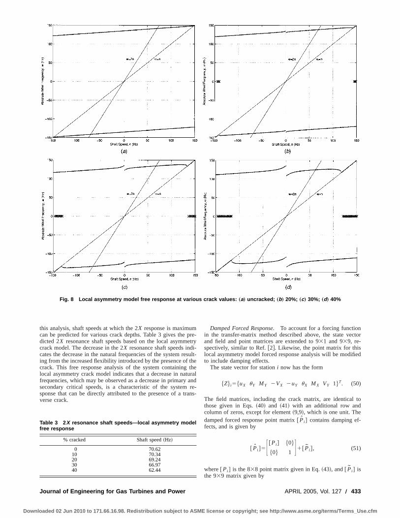
this analysis, shaft speeds at which the 2X response is maximumcan be predicted for various crack depths. Table 3 gives the pre-dicted 2X resonance shaft speeds based on the local asymmetrycrack model. The decrease in the 2X resonance shaft speeds indi-cates the decrease in the natural frequencies of the system result-ing from the increased flexibility introduced by the presence of thecrack. This free response analysis of the system containing thelocal asymmetry crack model indicates that a decrease in naturalfrequencies, which may be observed as a decrease in primary andsecondary critical speeds, is a characteristic of the system re-sponse that can be directly attributed to the presence of a trans-verse crack.

Damped Forced Response.To account for a forcing functionin the transfer-matrix method described above, the state vectorand field and point matrices are extended to 931 and 939, re-spectively, similar to Ref.@2#. Likewise, the point matrix for thislocal asymmetry model forced response analysis will be modifiedto include damping effects.

The state vector for stationi now has the form

$Z% i5$uX uY MY 2VX 2uY uX MX VY 1%T. (50)

The field matrices, including the crack matrix, are identical tothose given in Eqs.~40! and ~41! with an additional row andcolumn of zeros, except for element~9,9!, which is one unit. Thedamped forced response point matrix@ Pi # contains damping ef-fects, and is given by

@ Pi #5F @Pi # $0%

$0% 1 G1@ Pi #, (51)

where@Pi # is the 838 point matrix given in Eq.~43!, and@ Pi # isthe 939 matrix given by

Fig. 8 Local asymmetry model free response at various crack values: „a… uncracked; „b… 20%; „c… 30%; „d… 40%

Table 3 2 X resonance shaft speeds—local asymmetry modelfree response


0 70.6210 70.3420 69.2430 66.9740 62.44



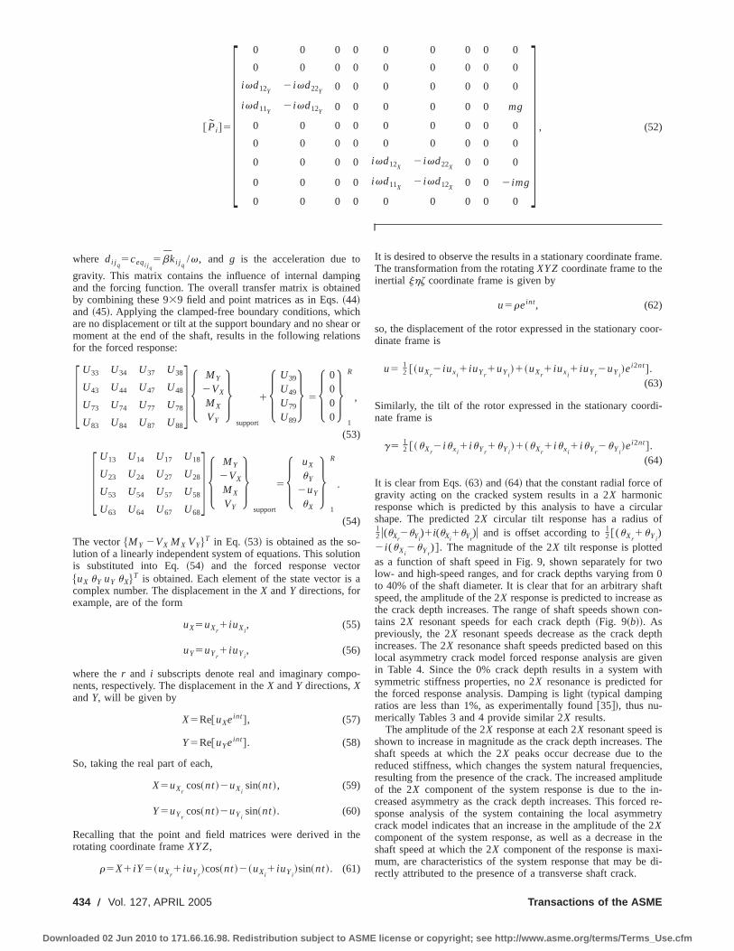
@ Pi #530 0 0 0 0 0 0 0 0

0 0 0 0 0 0 0 0 0

ivd12Y2 ivd22Y

0 0 0 0 0 0 0

ivd11Y2 ivd12Y

0 0 0 0 0 0 mg

0 0 0 0 0 0 0 0 0

0 0 0 0 0 0 0 0 0

0 0 0 0 ivd12X2 ivd22X

0 0 0

0 0 0 0 ivd11X2 ivd12X

0 0 2 img

0 0 0 0 0 0 0 0 0

4 , (52)

where di j q5ceqi j q

5bki j q/v, and g is the acceleration due to

gravity. This matrix contains the influence of internal dampingand the forcing function. The overall transfer matrix is obtainedby combining these 939 field and point matrices as in Eqs.~44!and ~45!. Applying the clamped-free boundary conditions, whichare no displacement or tilt at the support boundary and no shear ormoment at the end of the shaft, results in the following relationsfor the forced response:

FU33 U34 U37 U38

U43 U44 U47 U48

U73 U74 U77 U78

U83 U84 U87 U88

G H MY

2VX

MX

VY

Jsupport

1H U39

U49

U79

U89

J 5H 0000J

1

R

,

(53)

FU13 U14 U17 U18

U23 U24 U27 U28

U53 U54 U57 U58

U63 U64 U67 U68

G H MY

2VX

MX

VY

Jsupport

5H uX

uY

2uY

uX

J1

R

.

(54)

The vector$MY 2VX MX VY%T in Eq. ~53! is obtained as the so-lution of a linearly independent system of equations. This solutionis substituted into Eq.~54! and the forced response vector$uX uY uY uX%T is obtained. Each element of the state vector is acomplex number. The displacement in theX andY directions, forexample, are of the form

uX5uXr1 iuXi

, (55)

uY5uYr1 iuYi

, (56)

where ther and i subscripts denote real and imaginary compo-nents, respectively. The displacement in theX andY directions,XandY, will be given by

X5Re@uXeint#, (57)

Y5Re@uYeint#. (58)

So, taking the real part of each,

X5uXrcos~nt!2uXi

sin~nt!, (59)

Y5uYrcos~nt!2uYi

sin~nt!. (60)

Recalling that the point and field matrices were derived in therotating coordinate frameXYZ,

r5X1 iY5~uXr1 iuYr

!cos~nt!2~uXi1 iuYi

!sin~nt!. (61)

It is desired to observe the results in a stationary coordinate frame.The transformation from the rotatingXYZcoordinate frame to theinertial jhz coordinate frame is given by

u5reint, (62)

so, the displacement of the rotor expressed in the stationary coor-dinate frame is

u512 @~uXr

2 iuxi1 iuYr

1uYi!1~uXr

1 iuxi1 iuYr

2uYi!ei2nt#.

(63)

Similarly, the tilt of the rotor expressed in the stationary coordi-nate frame is

g512 @~uXr

2 iuxi1 iuYr

1uYi!1~uXr

1 iuxi1 iuYr

2uYi!ei2nt#.

(64)

It is clear from Eqs.~63! and~64! that the constant radial force ofgravity acting on the cracked system results in a 2X harmonicresponse which is predicted by this analysis to have a circularshape. The predicted 2X circular tilt response has a radius of12 u(uXr

2uYi)1i(uXi

1uYr)u and is offset according to12 @(uXr

1uYi)

2 i (uXi2uYr

)#. The magnitude of the 2X tilt response is plottedas a function of shaft speed in Fig. 9, shown separately for twolow- and high-speed ranges, and for crack depths varying from 0to 40% of the shaft diameter. It is clear that for an arbitrary shaftspeed, the amplitude of the 2X response is predicted to increase asthe crack depth increases. The range of shaft speeds shown con-tains 2X resonant speeds for each crack depth~Fig. 9~b!!. Aspreviously, the 2X resonant speeds decrease as the crack depthincreases. The 2X resonance shaft speeds predicted based on thislocal asymmetry crack model forced response analysis are givenin Table 4. Since the 0% crack depth results in a system withsymmetric stiffness properties, no 2X resonance is predicted forthe forced response analysis. Damping is light~typical dampingratios are less than 1%, as experimentally found@35#!, thus nu-merically Tables 3 and 4 provide similar 2X results.

The amplitude of the 2X response at each 2X resonant speed isshown to increase in magnitude as the crack depth increases. Theshaft speeds at which the 2X peaks occur decrease due to thereduced stiffness, which changes the system natural frequencies,resulting from the presence of the crack. The increased amplitudeof the 2X component of the system response is due to the in-creased asymmetry as the crack depth increases. This forced re-sponse analysis of the system containing the local asymmetrycrack model indicates that an increase in the amplitude of the 2Xcomponent of the system response, as well as a decrease in theshaft speed at which the 2X component of the response is maxi-mum, are characteristics of the system response that may be di-rectly attributed to the presence of a transverse shaft crack.



4 ConclusionsTwo theoretical analyses have been presented to identify char-

acteristics of the system response that may be directly attributed tothe presence of a transverse crack in the shaft of the test rigsystem. Both the global and local asymmetry crack model analy-ses qualitatively predict response characteristics which have beenexperimentally observed in the response of a system containing agaping crack.

The behavior of the 2X harmonic component of the systemresponse is an effective target observation for a monitoring sys-tem. The predicted behaviors of the 2X harmonic component of

the system response include an increase in magnitude for increas-ing crack depth as well as a decrease in the shaft speed at whichthe 2X harmonic component of the system response is maximum.The presence of a transverse shaft crack has also been shown toinduce an unstable response for some shaft speeds. The detectionof changes in the magnitude of the 2X harmonic component of thesystem response becomes much more difficult for shaft speedswhich are greater than 2X resonance speeds. Frequency-sweeptests, which pass through 2X resonance shaft speeds, would pro-vide the most useful information; however, observation of themagnitude of the 2X component could also provide crack diag-nostic information.

This research utilizes a method to account for a shaft crack inthe transfer-matrix method. By employing these transfer matrices,coupled systems that include shafts, seals, bearings, etc., can besystematically analyzed in a modular fashion@2#.

AcknowledgmentsThis research was conducted under Grant No. N00014-95-1-

0539 of the Office of Naval Research. Dr. Peter Schmidt was theProgram Manger. This support is gratefully acknowledged.

Appendix: Asymmetric StiffnessThe stiffness elements relate the displacement and tilt at the end

of the shaft to the applied forces or moments in theX and Ydirections. The stiffness relationships for a cantilever Euler-Bernoulli beam are obtained from general beam theory as

H FX

MYJ 5F k11Y

2k12Y

2k21Yk22Y

G H XgY

J (A1)

and

H FY

MXJ 5F k11X

k12X

k21Xk22X

G H YgX

J , (A2)

where k11X512EIX / l 3, k12X

5k21X56EIX / l 2, k22X

54EIX / l ,

k11Y512EIY / l 3, k12Y

5k21Y56EIY / l 2, andk22Y

54EIY / l .The area moments of inertia,I, are calculated about theX andY

axes. For the uncracked case, theX andY axes are also the neutralaxes of bending.

The asymmetric stiffness relationships are obtained by calculat-ing the appropriate asymmetric area moments of inertia and prop-erly substituting them into the stiffness coefficientski j above.

The cross section of the shaft at the location of the crack, whichis shown in Fig. 10, has asymmetric area moments of inertia aboutthe neutral axes of bending which are parallel to theX andY axes.To find the area moments of inertia about the neutral axes ofbending, the parallel axis theorem was utilized.

Fig. 9 Local asymmetry model forced response: „a… low-speedrange; „b… high-speed range

Fig. 10 Asymmetric shaft cross section

Table 4 2 X resonance shaft speeds—local asymmetry modelforced response


010 70.3420 69.2430 66.9740 62.44



The area moments of inertia about theX andY axes,I X and I Y ,are defined as

I X5EAY2dA5E

AY2dXdY, (A3)

I Y5EAX2dA5E

AX2dXdY, (A4)

where A is the uncracked area of the cross section. The cross-coupled area moments of inertia,I XY and I YX , are zero since theX axis is an axis of symmetry. After integrating over the un-cracked area, the following equations forI X and I Y result:

I X5pr 4

81

1

4 F ~r 2a!~r 224ra12a2!A2ra2a2

1r 4 sin21S r 2a

r D G , (A5)

I Y5pr 4

41

~r 2a!~2Y!3

122

1

4 FY~2Y22r 2!Ar 22Y2

1r 4 sin21S Y

r D G , (A6)

where r is the shaft radius,a is the crack depth, andY5Aa(2r 2a) for convenience.

The following expressions for the area of the cross section,A,and the distance from theX axis to the centroid of the crosssection,X, can be obtained

A5~r 2a!A2ra2a21r 2 sin21S 12a

r D1pr 2

2, (A7)

X52

3A~2ar2a2!3/2. (A8)

The moments of inertia about the parallel centroidal axes,I X andI Y , are then obtained according to the parallel axis theorem as

I X5 I X , (A9)

I Y5 I Y2AX2. (A10)

References@1# Zou, M., Dayan, J., and Green, I., 2000, ‘‘Dynamic Simulation and Monitoring

of a Non-Contacting Flexibly Mounted Rotor Mechanical Face Seal,’’ IMechE,Proc. Inst. Mech. Eng.214~C9!, Part C, pp. 1195–1206.

@2# Lee, A. S., and Green, I., 1994, ‘‘Rotordynamics of a Mechanical Face SealRiding on a Flexible Shaft,’’ ASME J. Tribol.,116~2!, pp. 345–351.

@3# Lee, A. S., and Green, I., 1994, ‘‘Higher Harmonic Oscillations in a Noncon-tacting FMR Mechanical Face Seal Test Rig,’’ ASME J. Vibr. Acoust.,116~2!,pp. 161–167.

@4# Lee, A. S., and Green, I., 1995, ‘‘An Experimental Investigation of the Steady-State Response of a Noncontacting Flexibly Mounted Rotor Mechanical FaceSeal,’’ ASME J. Tribol.,117~1!, pp. 153–159.

@5# Lee, A. S., and Green, I., 1995, ‘‘Physical Modeling and Data Analysis of theDynamic Response of a Flexibly Mounted Rotor Mechanical Seal,’’ ASME J.Tribol., 117, pp. 130–135.

@6# Zou, M., and Green, I., 1999, ‘‘Clearance Control of a Mechanical Face Seal,’’STLE Tribol. Trans.,42, pp. 535–540.

@7# Zou, M., Dayan, J., and Green, I., 1999, ‘‘Parametric Analysis of ContactControl of a Noncontacting Mechanical Face Seal,’’ inProceedings of Vibra-tion, Noise and Structural Dynamics, pp. 493–499, April.

@8# Dayan, J., Zou, M., and Green, I., 2000, ‘‘Sensitivity Analysis for the Designand Operation of a Noncontacting Mechanical Face Seal,’’ IMechE, Proc. Inst.Mech. Eng.214~C9!, Part C, pp. 1207–1218.

@9# Zou, M., Dayan, J., and Green, I., 2000, ‘‘Feasibility of Contact Elimination ofa Mechanical Face Seal Through Clearance Adjustment,’’ ASME J. Eng. GasTurbines Power,122, pp. 478–484.

@10# Dayan, J., Zou, M., and Green, I., 1999, ‘‘Contact Elimination in MechanicalFace Seals Using Active Control,’’ inProceedings of the IEEE 7th Mediterra-nean Conference on Control and Automation (MED99), pp. 618–619, June.

@11# Tondl, A., 1965,Some Problems in Rotor Dynamics, Czechoslovakian Acad-emy of Sciences, Chapman & Hall, London.

@12# Henry, T. A., and Okah-Avae, B. E., 1976, ‘‘Vibrations in Cracked Shafts,’’ inConference on Vibrations in Rotating Machinery, pp. 15–19.

@13# Murray, D. B., and McCraith, J. R., 1984, ‘‘Vibrational Method for the Detec-tion of Cracks in Rotating Shafts,’’ inFirst Parsons International TurbineConference, pp. 229–236.

@14# Rao, J. S., 1991,Rotor Dynamics, 2nd edition, Wiley, New York.@15# Gasch, R., 1976, ‘‘Dynamic Behavior of Simple Rotor With a Cross-Sectional

Crack,’’ in Conference on Vibrations in Rotating Machinery, p. 123.@16# Mayes, I. W., and Davies, W. G. R., 1976, ‘‘The Vibrational Behavior of a

Rotating Shaft System Containing a Transverse Crack,’’ inConference onVibrations in Rotating Machinery, pp. 53–64.

@17# Imam, I., and Azzaro, S. H., 1989, ‘‘Development of an On-Line Rotor CrackDetection and Monitoring System,’’ ASME J. Vib., Acoust., Stress, Reliab.Des.,111~3!, pp. 241–250.

@18# Huang, S. C., Huang, Y. M., and Shieh, S. M., 1993, ‘‘Vibration and Stabilityof a Rotating Shaft Containing a Transverse Crack,’’ J. Sound Vib.,162, pp.387–401.

@19# Tsai, T., and Wang, W., 1998, ‘‘Vibration of a Rotor With a Transverse OpenCrack,’’ Proc. Natl. Sci. Counc., Repub. China, Part A: Phys. Sci. Eng.,22, pp.372–384.

@20# Grabowski, B., 1980, ‘‘The Vibrational Behavior of a Turbine Rotor Contain-ing a Transverse Crack,’’ ASME J. Mech. Des.,121, pp. 140–146.

@21# Dimarogonas, A. D., and Paipetis, S. A., 1983,Analytical Methods in RotorDynamics, Applied Science.

@22# Herbert, R. G., 1987, ‘‘Turbine-Alternator Run-Down Vibration Analysis: Au-tomated Crack Detection,’’ in11th Biennial Conference on Mechanical Vibra-tion and Noise, Vol. 2, pp. 631–636.

@23# Inagaki, T., Kanki, H., and Shiraki, K., 1982, ‘‘Transverse Vibrations of aGeneral Cracked-Rotor Bearing System,’’ ASME J. Mech. Des.,104~2!, pp.345–355.

@24# Schmied, J., and Kraemer, E., 1984, ‘‘Vibrational Behavior of a Rotor With aCross-Sectional Crack,’’ inConference on Vibrations in Rotating Machinery,pp. 183–192.

@25# Nelson, H. D., and Nataraj, C., 1986, ‘‘The Dynamics of a Rotor System Witha Cracked Shaft,’’ ASME J. Vib., Acoust., Stress, Reliab. Des.,108, pp. 189–196.

@26# Sofker, D., Bajkowski, J., and Muller, P. C., 1993, ‘‘Crack Detection in TurboRotors, Vibrational Analysis and Fault Detection,’’ inConference on Mechani-cal Vibration and Noise, Vol. 60, pp. 277–287.

@27# Meng, G., and Hahn, E. J., 1994, ‘‘Dynamic Response of a Cracked RotorWith Some Comments on Crack Detection,’’ inProceedings of the Interna-tional Gas Turbine and Aeroengine Congress and Exposition, June.

@28# Dirr, B. O., and Rothkegel, W., 1994, ‘‘Detection and Simulation ofSmall Transverse Cracks in Rotating Shafts,’’ Arch. Appl. Mech.,64~3!,pp. 206–222.

@29# Inagaki, T., Kanki, H., and Shiraki, K., 1980, ‘‘Response Analysis of a GeneralAsymmetric Rotor-Bearing,’’ ASME J. Mech. Des.,102~1!, pp. 147–157.

@30# Dimarogonas, A. D., and Papadopoulos, C. A., 1983, ‘‘Vibration of CrackedShafts in Bending,’’ J. Sound Vib.,91, pp. 583–593.

@31# Davies, W. G. R., and Mayes, I. W., 1984, ‘‘The Vibrational Behavior of aMulti-Shaft, Multi-Bearing System in the Presence of a Propogating Trans-verse Crack,’’ ASME J. Vib., Acoust., Stress, Reliab. Des.,106~1!, pp. 146–153.

@32# Gasch, R., 1993, ‘‘A Survey of the Dynamic Behavior of a Simple RotatingShaft With a Transverse Crack,’’ J. Sound Vib.,160, pp. 313–332.

@33# Papadopoulos, C. A., and Dimarogonas, A. D., 1987, ‘‘Stability of CrackedRotors in the Coupled Vibration Mode,’’ in11th Biennial Conference on Me-chanical Vibration and Noise, Vol. 1, pp. 25–34.

@34# Papadopoulos, C. A., and Dimarogonas, A. D., 1987, ‘‘Coupled Longitudinaland Bending Vibrations of a Rotating Shaft With an Open Crack,’’ J. SoundVib., 117, pp. 81–93.

@35# Casey, C., 2000, ‘‘Crack Detection in Rotor Dynamic System by VibrationMonitoring,’’ M.S. thesis, Georgia Institute of Technology.

@36# Green, I., and Etsion, I., 1986, ‘‘A Kinematic Model for Mechanical SealsWith Antirotation Locks or Positive Drive Devices,’’ ASME J. Tribol.,108~1!,pp. 42–45.

@37# Tada, H., Paris, P. C., and Irwin, G. R., 1985,The Stress Analysis of CracksHandbook, 2nd Ed., Paris Productions, St. Lous, MO.



Andrew J. ProvenzaNASA Glenn Research Center,

Cleveland, OH 44135-3191e-mail: [email protected]

Gerald T. MontagueArmy Research Lab,

NASA Glenn Research Center,Cleveland, OH 44135


Mark J. JansenUniversity of Toledo,

Toledo, OHe-mail: [email protected]

Alan B. PalazzoloDepartment of Mechanical Engineering,

Texas A&M University,College Station, TX


Ralph H. JansenUniversity of Toledo,

Toledo, OHe-mail: [email protected]

High TemperatureCharacterization of a RadialMagnetic Bearing forTurbomachineryOpen loop, experimental force and power measurements of a radial, redundant-axis,magnetic bearing at temperatures to 1000°F (538°C) and rotor speeds to 15,000 rpmalong with theoretical temperature and force models are presented in this paper. Theexperimentally measured force produced by a single C-core circuit using 22A was 600 lb(2.67 kN) at room temperature and 380 lb (1.69 kN) at 538°C. These values were com-pared with force predictions based on a one-dimensional magnetic circuit analysis and athermal analysis of gap growth as a function of temperature. The analysis showed that thereduction of force at high temperature is mostly due to an increase in radial gap due totest conditions, rather than to reduced core permeability. Tests under rotating conditionsshowed that rotor speed has a negligible effect on the bearing’s static force capacity. OneC-core required approximately 340 W of power to generate 190 lb (845 N) of magneticforce at 538°C, however the magnetic air gap was much larger than at room temperature.The data presented are after bearing operation for eleven total hours at 538°C and sixthermal cycles.@DOI: 10.1115/1.1807413#

Introduction

The gas turbine industry has a continued vested interest in im-proving engine performance and reducing net operating and main-tenance costs. These goals are being realized because of advance-ments in materials, aeroelasticity & CFD analysis, and enginesimulation. These advancements also aid in increasing enginethrust-to-weight ratios, pressure ratios, specific fuel consumption,and overall reliability through higher-efficiency engine operationat higher rotational speeds and temperatures.

Rolling element bearings and squeeze film dampers are cur-rently used to support gas turbine engine rotors. These types ofbearings are limited in temperature~,260°C! and speed~,2.5million DN! and require both cooling air and a lubrication system.Rolling element bearings in gas turbines have been pushed to theirlimits and new bearing technologies must be developed to takefull advantage of other aforementioned advancements.

Magnetic bearings are well suited to operate at elevated tem-perature, higher rotational speeds, and extreme altitudes~thin airatmosphere! and are a promising solution to current limitations.

Magnetic bearings in gas turbine engines would eliminate lu-brication analysis, leaks, spills, contamination, and unnecessarymaintenance due to faulty chip detection. The magnetic bearingcould also provide health monitoring and adapt the rotor supportto actively respond to transients such as hard aircraft landings andsudden imbalances. Magnetic bearings will enable engine design-ers to take full advantage of other technological advancements inturbine engine components by allowing rotor components to spinat higher speeds and at higher temperatures. As a result, turbineand compressor spools can be designed with higher operatingtemperatures and with significantly larger, faster, stiffer, highlydamped rotors.

Literature SearchMagnetic bearing technology is being developed worldwide

and is considered an enabling technology for new, hotter enginedesigns. There are several institutions which have been develop-ing hardware for this high temperature application. Xu, Wang, andSchweitzer demonstrated 1 degree-of-freedom~DOF! levitation ofa plate at 560°C and presented a design of a magnetic bearingsystem for 5 DOF in Ref.@1#. Vibration results for a blower usedto recycle 700°C cathode gas, fully suspended by magnetic bear-ings operating at 400°C, was presented by Ohsawa et al.@2#Mekhiche et al. developed a high temperature magnetic bearingsystem that is described from design through room temperaturetesting in Refs.@3,4#. Field et al. described a complete, reliablemagnetic bearing system targeted for high temperature applicationin Refs. @5,6#. Only in Ref. @2# can actual experimental data de-scribing high temperature operation be found. But the data de-scribe the vibration response of the suspended rotor at tempera-ture. They do not present an assessment of the effects oftemperature on magnetic bearing properties and system require-ments.

High temperature magnetic properties of candidate magneticmaterials were investigated in the 1960s by Kueser et al.@7#, andrecently by Kondoleon and Kelleher@8# and Fingers@9#. Hyperco50 data in Ref.@7# does not indicate a significant decrease inpermeability or saturation flux density at 538°C.

After reviewing the available literature, the authors believe thatthis paper provides the first baseline industry performance charac-teristics for actual magnetic bearing hardware during operation attemperatures up to 538°C.

The third generation high temperature, high load magnetic bear-ing, developed at the NASA Glenn Research Center, was firstcharacterized at room temperature~RT! up to 20,000 rpm. It iscapable of producing over 1000 lb~4.5 kN! of force per magneticaxis at RT and at speed. RT data for this bearing is presented inRef. @10#.

Data presented in this paper characterizes the third generationbearing at temperatures up to 538°C. Bearing force as a functionof current, temperature, and speed to 15,000 rpm is shown. Bear-




ing power consumption measurements taken at several appliedcurrents and temperatures are also presented. And finally, resultsof a simple analytical model are compared to the experimentalforce results.

Test Facility

Facility Description. The high temperature magnetic bearingtest facility is shown in Fig. 1. The structural support can accom-modate thrust and radial bearings up to 22.8 cm diameter with amaximum axial loading of 22 kN and a maximum radial loadingof 11.1 kN. The test facility has been configured a number ofdifferent ways@10,11#.

The current configuration can be seen in Fig. 2. The magneticbearing is located at the center of gravity of the 75-mm-diam rotorthat weighs 8 kg. The 200-mm-diam stator weighs 23 kg. A 0.56mm radial air gap exists between the stator poles and the rotor atRT. The rotor has interchangeable sleeves on each end that inter-face it with the support bearings, which, for these tests, are high-speed, grease packed, duplex ball bearings. For this configuration,the rotor was fitted with negative clearance sleeves so it was sup-ported on pre-loaded ball bearings at both ends. This was done sothat forces exerted by the magnetic bearing could be easily anddirectly measured outside the hot section at the support bearinglocations. The outboard sleeve can be replaced with a positiveclearance sleeve so that the magnetic bearing can support the ro-tor. An air turbine drives the rotor.

The magnetic bearing stator is an isolated C-core, 12-pole, het-eropolar design, and is described in detail in Ref.@12#. The stator

has an axial length of 76 mm. Each C-core is wrapped with twocoils of 52 turns each of specially insulated and potted silver wire.

Power to the magnetic bearing is provided through tri-state,pulse width modulated~PWM! amplifiers. These components arepassively filtered to remove high frequency amplifier noise thatresults from hard amplifier switching and for reducing EMI emis-sions from the bearing coils that are picked up by the eddy currentposition sensors.

Heat is supplied to the bearing through three, 3 kW band heat-ers wrapped around the stator~Fig. 2!. Ground Fault Circuit In-terrupts~GFCIs! have been incorporated into the heating systemand the PWM amplifier circuits to protect the hardware and forsafeguarding personnel. The facility is described in more detail inRef. @12#. Figure 3 shows the facility at 538°C with the statorglowing ‘‘orange’’ hot.

Sensors. The facility is equipped with several different typesof sensors that monitor load, temperature, rotor position, speed,and electric current.

High load, high bandwidth, piezoelectric load cells, with anaccuracy of61.5 N, support the inboard and outboard rollingelement bearings~Fig. 4!. These load cells are capable of measur-ing loads up to 7.5 kN at 200 kHz and have a maximum operatingtemperature of 200°C. Two load cells are aligned along each ofthe three magnetic bearing axes on both support bearings for atotal of 12 load cells. Each load cell was set with a preload of 1kN. This preload value supplied symmetric structural rotor sup-port, put the critical speed out of the operating range, and estab-

Fig. 1 High-temperature magnetic bearing test facility atNASA Glenn Research Center

Fig. 2 Third-generation high-temperature magnetic bearingtest rig

Fig. 3 Magnetic bearing at 538°C „1000°F…

Fig. 4 Six load cells supporting the outboard duplex ball bear-ing



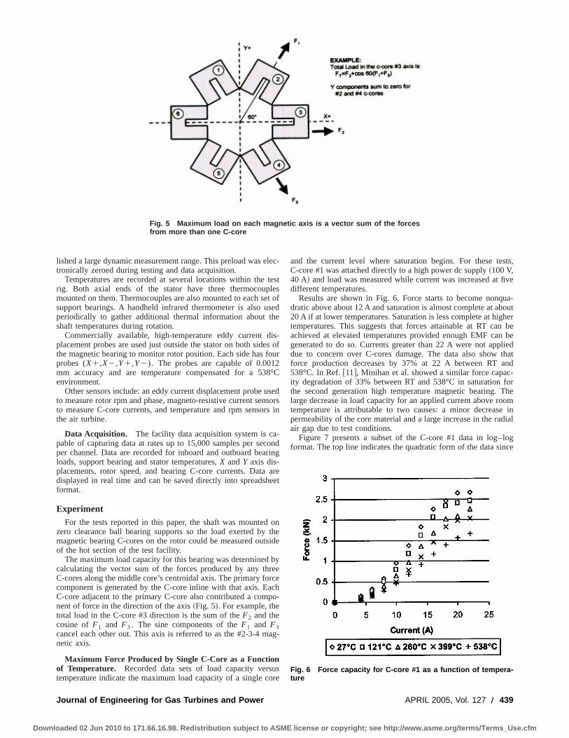
lished a large dynamic measurement range. This preload was elec-tronically zeroed during testing and data acquisition.

Temperatures are recorded at several locations within the testrig. Both axial ends of the stator have three thermocouplesmounted on them. Thermocouples are also mounted to each set ofsupport bearings. A handheld infrared thermometer is also usedperiodically to gather additional thermal information about theshaft temperatures during rotation.

Commercially available, high-temperature eddy current dis-placement probes are used just outside the stator on both sides ofthe magnetic bearing to monitor rotor position. Each side has fourprobes (X1,X2,Y1,Y2). The probes are capable of 0.0012mm accuracy and are temperature compensated for a 538°Cenvironment.

Other sensors include: an eddy current displacement probe usedto measure rotor rpm and phase, magneto-resistive current sensorsto measure C-core currents, and temperature and rpm sensors inthe air turbine.

Data Acquisition. The facility data acquisition system is ca-pable of capturing data at rates up to 15,000 samples per secondper channel. Data are recorded for inboard and outboard bearingloads, support bearing and stator temperatures,X andY axis dis-placements, rotor speed, and bearing C-core currents. Data aredisplayed in real time and can be saved directly into spreadsheetformat.

ExperimentFor the tests reported in this paper, the shaft was mounted on

zero clearance ball bearing supports so the load exerted by themagnetic bearing C-cores on the rotor could be measured outsideof the hot section of the test facility.

The maximum load capacity for this bearing was determined bycalculating the vector sum of the forces produced by any threeC-cores along the middle core’s centroidal axis. The primary forcecomponent is generated by the C-core inline with that axis. EachC-core adjacent to the primary C-core also contributed a compo-nent of force in the direction of the axis~Fig. 5!. For example, thetotal load in the C-core #3 direction is the sum of theF2 and thecosine ofF1 and F3 . The sine components of theF1 and F3cancel each other out. This axis is referred to as the #2-3-4 mag-netic axis.

Maximum Force Produced by Single C-Core as a Functionof Temperature. Recorded data sets of load capacity versustemperature indicate the maximum load capacity of a single core

and the current level where saturation begins. For these tests,C-core #1 was attached directly to a high power dc supply~100 V,40 A! and load was measured while current was increased at fivedifferent temperatures.

Results are shown in Fig. 6. Force starts to become nonqua-dratic above about 12 A and saturation is almost complete at about20 A if at lower temperatures. Saturation is less complete at highertemperatures. This suggests that forces attainable at RT can beachieved at elevated temperatures provided enough EMF can begenerated to do so. Currents greater than 22 A were not applieddue to concern over C-cores damage. The data also show thatforce production decreases by 37% at 22 A between RT and538°C. In Ref.@11#, Minihan et al. showed a similar force capac-ity degradation of 33% between RT and 538°C in saturation forthe second generation high temperature magnetic bearing. Thelarge decrease in load capacity for an applied current above roomtemperature is attributable to two causes: a minor decrease inpermeability of the core material and a large increase in the radialair gap due to test conditions.

Figure 7 presents a subset of the C-core #1 data in log–logformat. The top line indicates the quadratic form of the data since

Fig. 5 Maximum load on each magnetic axis is a vector sum of the forcesfrom more than one C-core

Fig. 6 Force capacity for C-core #1 as a function of tempera-ture



each temperature data set is almost parallel to it. If the gap dimen-sion was independent of temperature, then these curves would lineup on top of each other. However, the actual gap dimension ateach temperature can be backed out of this data using the assump-tion that the change in relative permeability of the core material isnegligible and provided the initial gap at room temperature isknown. Magnetization curves for 0.1 mm laminations of Hiperco50 alloy in Ref. @7# do not appear to indicate an appreciablechange with temperature~RT to 538°C! in relative permeability orinduction for a fixed magnetizing force.

An inherent increase in gap length exists based solely upon thefact that the magnetic bearing lamination stacks are heating up. Ifthe change in temperature of both the rotor and the stator is uni-form, the gap grows by 0.5% at 538°C. One way to see thisincrease is to imagine replacing the air in the gap with laminationmaterial. After applying heat, not only due the rotor and statorstacks expand, but so too does the gap material. Since this imagi-nary gap stack does not affect the growth of either the stator or therotor stack, it can be concluded that the gap grows with tempera-ture by a small amount as does the other metal components.

The coefficient of thermal expansion for Hyperco 50 is 5.2831026 in./~in. °F) and the gap is 0.022 in. An increase of 538°Cthus results in a 0.5% increase in gap length, which results in a1% loss in force capacity.

Individual C-Core Force Capacity as a Function of Speedand Temperature. Typical load capacity of a single C-core as afunction of current, temperature, and speed is presented here.C-core #2 load capacity data at 0 and 15,000 rpm from 27 to538°C is shown in Figs. 8 and 9.

The data show that speed does not have an appreciable effect onthe force capacity of C-core #2 at any temperature or speed to15,000 rpm. This same result was observed previously in Ref.@10#.

Figure 10 shows just how close the data matches at 538°C.Slight variations are most likely associated with the timeliness ofthe measurements. Gap size affects these measurements and howlong the stator took to get from RT to 538°C and how long it wasthere is critical. Possible nonuniform frictional forces generatedwithin the rolling element bearings as the rotor gets hot, which arenot accounted for, may also be a source of variation. Small netfrictional forces in the direction of load could develop if the pre-loads are not perfectly balanced, or if the concentricity between

the rotor and the outboard rolling element bearing changes. How-ever, the ball bearings do provide a good load path from the ro-tating shaft and this effect seems minimal.

The option of measuring forces directly at the stator~Fig. 11!has been tried, with difficulty, prior to this publication. The mainproblem was that the load cells had to be in line with the statormechanical support and an external actuator system was required.This support configuration permitted unwanted stator deflectionand position slip during dynamic tests.

As the speed increases, rotor eddy current and hysteresis lossesincrease. However, these losses do not affect the static load pro-duction capability of this bearing at elevated temperatures to15,000 rpm. These losses still have negative effects on actuatorbandwidth.

For this particular C-core, a decrease in load capacity of 53% isevident at 15 A between RT and 538°C. This is considerablyhigher than previous results have shown. Since force is propor-tional to the inverse square of the total air gap, small changes inair gap can greatly affect bearing output for any current values. Itwould appear that Figs. 8 and 9 would have shown a more favor-able result if data from C-core #1 was recorded. However, it ishighly unlikely that the test rig reached an equilibrium tempera-ture when Fig. 6 data were recorded.

Fig. 7 C-core #1 force data plotted on log–log plotFig. 8 Force vs current for C-core #2 at 0 rpm

Fig. 9 Force vs current for C-core #2 at 15,000 rpm



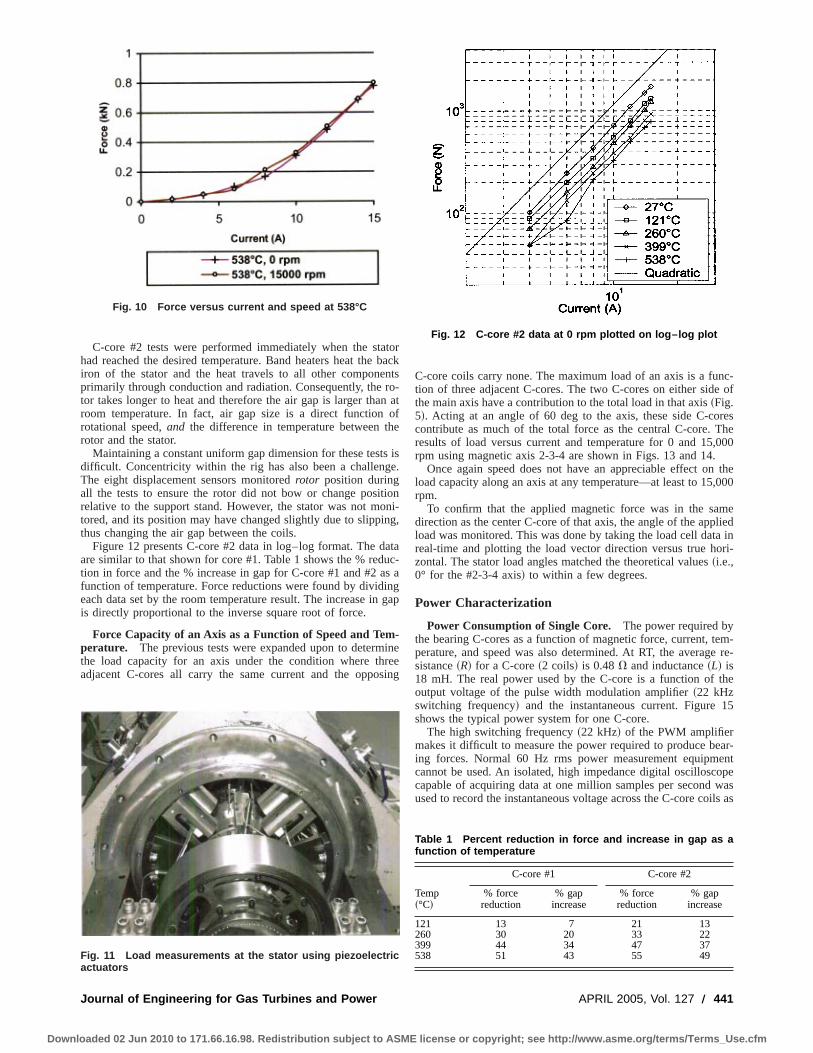
C-core #2 tests were performed immediately when the statorhad reached the desired temperature. Band heaters heat the backiron of the stator and the heat travels to all other componentsprimarily through conduction and radiation. Consequently, the ro-tor takes longer to heat and therefore the air gap is larger than atroom temperature. In fact, air gap size is a direct function ofrotational speed,and the difference in temperature between therotor and the stator.

Maintaining a constant uniform gap dimension for these tests isdifficult. Concentricity within the rig has also been a challenge.The eight displacement sensors monitoredrotor position duringall the tests to ensure the rotor did not bow or change positionrelative to the support stand. However, the stator was not moni-tored, and its position may have changed slightly due to slipping,thus changing the air gap between the coils.

Figure 12 presents C-core #2 data in log–log format. The dataare similar to that shown for core #1. Table 1 shows the % reduc-tion in force and the % increase in gap for C-core #1 and #2 as afunction of temperature. Force reductions were found by dividingeach data set by the room temperature result. The increase in gapis directly proportional to the inverse square root of force.

Force Capacity of an Axis as a Function of Speed and Tem-perature. The previous tests were expanded upon to determinethe load capacity for an axis under the condition where threeadjacent C-cores all carry the same current and the opposing

C-core coils carry none. The maximum load of an axis is a func-tion of three adjacent C-cores. The two C-cores on either side ofthe main axis have a contribution to the total load in that axis~Fig.5!. Acting at an angle of 60 deg to the axis, these side C-corescontribute as much of the total force as the central C-core. Theresults of load versus current and temperature for 0 and 15,000rpm using magnetic axis 2-3-4 are shown in Figs. 13 and 14.

Once again speed does not have an appreciable effect on theload capacity along an axis at any temperature—at least to 15,000rpm.

To confirm that the applied magnetic force was in the samedirection as the center C-core of that axis, the angle of the appliedload was monitored. This was done by taking the load cell data inreal-time and plotting the load vector direction versus true hori-zontal. The stator load angles matched the theoretical values~i.e.,0° for the #2-3-4 axis! to within a few degrees.

Power Characterization

Power Consumption of Single Core. The power required bythe bearing C-cores as a function of magnetic force, current, tem-perature, and speed was also determined. At RT, the average re-sistance~R! for a C-core~2 coils! is 0.48V and inductance~L! is18 mH. The real power used by the C-core is a function of theoutput voltage of the pulse width modulation amplifier~22 kHzswitching frequency! and the instantaneous current. Figure 15shows the typical power system for one C-core.

The high switching frequency~22 kHz! of the PWM amplifiermakes it difficult to measure the power required to produce bear-ing forces. Normal 60 Hz rms power measurement equipmentcannot be used. An isolated, high impedance digital oscilloscopecapable of acquiring data at one million samples per second wasused to record the instantaneous voltage across the C-core coils as

Fig. 10 Force versus current and speed at 538°C

Fig. 11 Load measurements at the stator using piezoelectricactuators

Fig. 12 C-core #2 data at 0 rpm plotted on log–log plot

Table 1 Percent reduction in force and increase in gap as afunction of temperature

Temp~°C!

C-core #1 C-core #2

% forcereduction

% gapincrease

% forcereduction

% gapincrease

121 13 7 21 13260 30 20 33 22399 44 34 47 37538 51 43 55 49



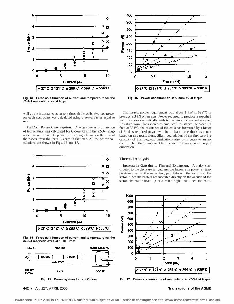
well as the instantaneous current through the coils. Average powerfor each data point was calculated using a power factor equal toone.

Full Axis Power Consumption. Average power as a functionof temperature was calculated for C-core #2 and the #2-3-4 mag-netic axis at 0 rpm. The power for the magnetic axis is the sum ofthe power from the three C-cores in that axis. All the power cal-culations are shown in Figs. 16 and 17.

The largest power requirement was about 1 kW at 538°C toproduce 2.3 kN on an axis. Power required to produce a specifiedload increases dramatically with temperature for several reasons.Resistive power loss increases since coil resistance increases. Infact, at 538°C, the resistance of the coils has increased by a factorof 3, thus required power will be at least three times as muchbased on this result alone. Slight degradation of the flux carryingcapacity of the magnetic laminations also contributes to an in-crease. The other component here stems from an increase in gapdimension.

Thermal Analysis

Increase in Gap due to Thermal Expansion. A major con-tributor to the decrease in load and the increase in power as tem-perature rises is the expanding gap between the rotor and thestator. Since the heaters are mounted directly on the outside of thestator, the stator heats up at a much higher rate then the rotor,

Fig. 13 Force as a function of current and temperature for the#2-3-4 magnetic axes at 0 rpm

Fig. 14 Force as a function of current and temperature for the#2-3-4 magnetic axes at 15,000 rpm

Fig. 15 Power system for one C-core

Fig. 16 Power consumption of C-core #2 at 0 rpm

Fig. 17 Power consumption of magnetic axis #2-3-4 at 0 rpm



which relies only on convection and radiation for heating. Thus,the rotor will not have expanded as much as the stator, and as aresult, the gap will be larger than nominal.

In hindsight, it would seem advantageous to heat the rotor aswell as the stator to alleviate thermal mismatch problems. Withthe current rig setup, however, this is not possible. Stresses gen-erated from thermal expansion of the zero clearance bearingsleeves might cause the ball bearings to seize up. In addition, thegrease used to lubricate these bearings is only rated to 135°C. In afuture build, the ball bearings will be replaced with high tempera-ture hydrostatic bearings to allow consideration of other heatingmethods. The hydrostatic bearings will also allow for continuoustesting at higher speeds. Currently, the ball bearings heat upwithin minutes to their temperature limit in tests performed athigh speed.

Constant gap dimension is important in the determination offorce capacity and bearing power requirements, but the gap in areal engine application will not stay constant and could vary withtime and external environmental conditions, such as inlet airtemperature.

In order to better understand the growth of the gap, a linearthermal expansion analysis was conducted. The gap at any tem-perature has a minimum and maximum value just due to the tol-erance stack up of the rotor and stator bearing components. Theactual gap, which is somewhere between the max and min, willchange with thermal mismatch. Thermal maps of the magneticbearing section of the rotor were constructed using temperaturesmeasured at several different points on the rig using a handheldinfrared thermometer. Figure 18 shows that even after 2.5 h, theaverage gap dimension is greater than it is at room temperature. Itis quite possible, that the rotor would never reach 538°C using thecurrent heating method. The initial gap value for C-core #2 wasdetermined using plastic shims to be approximately 0.56 mm. Us-ing this reference and the values in Table 1, the actual gap can bedetermined. Values based on experiment and plotted in Fig. 18,fall between the max and min curves and thus provide confidencein the model.

The thermal map in Fig. 19 shows a temperature gradient on therotor. This gradient was due to different heating rates of each ofthe three band heaters and also because the outer containmentshell was removed for these tests allowing for convective cooling.The coolest rotor section is about 315°F. Figure 20 shows that therotor did reach a uniform temperature of about 415°C after 2.5 hof steady heating after the stator poles reached 538°C.

In this model, the average radial gap at room temperature was0.620 mm at 27°C. This gap increases to 0.792 mm at 538°C~Fig.18!. Since the magnetic force is a function of the inverse square ofthe gap distance~if core material is far from saturation!, it is clearwhy the force at elevated temperature severely drops for a fixedsupply current.

Force Prediction. A simple analytical prediction of force,made to verify the experimental results, is presented here. For ageneral magnetic actuator, the force produced by the magneticflux in one air gap of areaAg is

F51

2am0AgF NI

2G1L iron

m r

G 2

. (1)

In this equation,m0 is the magnetic permeability of free spaceandNI is the ampere-turns of the coil~s! driving flux through thecircuit. 2G represents the total effective magnetic air gap anda isa force de-rating factor, which accounts for leakage, fringing, andnon-uniformity in flux density across the pole face@13#. L iron rep-resents the average iron path component of the C-core circuit, andur is the relative permeability of the iron laminations.

The actuator measurements in this paper are based on the per-formance of a complete C-core circuit. Each of the two C-corepoles is 15° off-axis, therefore, the forced produced by a singleC-core is 1.93 times that obtained using Eq.~1!. Force predictionswere made using the following parameters:a50.8, m054p31027 N/A2, N55232 turns, Ag512.9 cm2, G050.559 mm,L iron5145 mm, m r5500. A nominalm r was calculated from thelocal slope of the Hyperco 50 data in Ref.@7# at 12 Oe and RT. 12Oe corresponds to about 10 A in these third generation radialbearing C-cores.

Figure 21 shows a comparison between the predicted force andthe measured force for C-core #1. An initial gap,G0 , of 0.47 mmwas used in the predictions since the force in C-core #1 wasconsiderably higher than that in C-core #2. The trend for gapincrease backed out of the measured data for C-core #1 shown inTable 1 was used to determine predicted gap values in C-core #1

Fig. 18 Theoretical gap between stator and rotor as a functionof temperature using linear method

Fig. 19 Thermal map „not FEA … of rotor and stator when rigfirst reaches 538°C

Fig. 20 Thermal map „not FEA … of rotor and stator after rig at538°C for 2.5 h



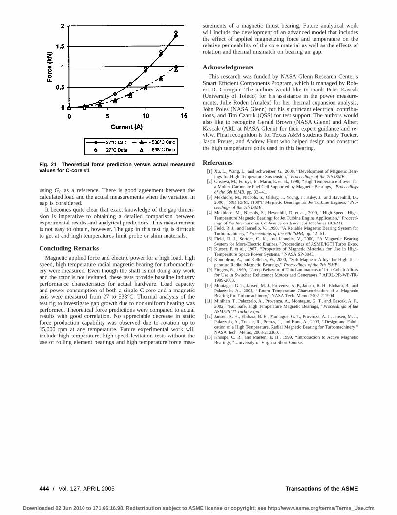
using G0 as a reference. There is good agreement between thecalculated load and the actual measurements when the variation ingap is considered.

It becomes quite clear that exact knowledge of the gap dimen-sion is imperative to obtaining a detailed comparison betweenexperimental results and analytical predictions. This measurementis not easy to obtain, however. The gap in this test rig is difficultto get at and high temperatures limit probe or shim materials.

Concluding RemarksMagnetic applied force and electric power for a high load, high

speed, high temperature radial magnetic bearing for turbomachin-ery were measured. Even though the shaft is not doing any workand the rotor is not levitated, these tests provide baseline industryperformance characteristics for actual hardware. Load capacityand power consumption of both a single C-core and a magneticaxis were measured from 27 to 538°C. Thermal analysis of thetest rig to investigate gap growth due to non-uniform heating wasperformed. Theoretical force predictions were compared to actualresults with good correlation. No appreciable decrease in staticforce production capability was observed due to rotation up to15,000 rpm at any temperature. Future experimental work willinclude high temperature, high-speed levitation tests without theuse of rolling element bearings and high temperature force mea-

surements of a magnetic thrust bearing. Future analytical workwill include the development of an advanced model that includesthe effect of applied magnetizing force and temperature on therelative permeability of the core material as well as the effects ofrotation and thermal mismatch on bearing air gap.

AcknowledgmentsThis research was funded by NASA Glenn Research Center’s

Smart Efficient Components Program, which is managed by Rob-ert D. Corrigan. The authors would like to thank Peter Kascak~University of Toledo! for his assistance in the power measure-ments, Julie Roden~Analex! for her thermal expansion analysis,John Poles~NASA Glenn! for his significant electrical contribu-tions, and Tim Czaruk~QSS! for test support. The authors wouldalso like to recognize Gerald Brown~NASA Glenn! and AlbertKascak~ARL at NASA Glenn! for their expert guidance and re-view. Final recognition is for Texas A&M students Randy Tucker,Jason Preuss, and Andrew Hunt who helped design and constructthe high temperature coils used in this bearing.

References@1# Xu, L., Wang, L., and Schweitzer, G., 2000, ‘‘Development of Magnetic Bear-

ings for High Temperature Suspension,’’Proceedings of the 7th ISMB.@2# Ohsawa, M., Furuya, E., Marui, E. et al., 1998, ‘‘High Temperature Blower for

a Molten Carbonate Fuel Cell Supported by Magnetic Bearings,’’Proceedingsof the 6th ISMB, pp. 32–41.

@3# Mekhiche, M., Nichols, S., Oleksy, J., Young, J., Kiley, J., and Havenhill, D.,2000, ‘‘50K RPM, 1100°F Magnetic Bearings for Jet Turbine Engines,’’Pro-ceedings of the 7th ISMB.

@4# Mekhiche, M., Nichols, S., Hevenhill, D. et al., 2000, ‘‘High-Speed, High-Temperature Magnetic Bearings for Jet Turbine Engine Application,’’Proceed-ings of the International Conference on Electrical Machines~ICEM!.

@5# Field, R. J., and Iannello, V., 1998, ‘‘A Reliable Magnetic Bearing System forTurbomachinery,’’Proceedings of the 6th ISMB, pp. 42–51.

@6# Field, R. J., Sortore, C. K., and Iannello, V., 2000, ‘‘A Magnetic BearingSystem for More-Electric Engines,’’ Proceedings of ASME/IGTI Turbo Expo.

@7# Kueser, P. et al., 1967, ‘‘Properties of Magnetic Materials for Use in High-Temperature Space Power Systems,’’ NASA SP-3043.

@8# Kondoleon, A., and Kelleher, W., 2000, ‘‘Soft Magnetic Alloys for High Tem-perature Radial Magnetic Bearings,’’Proceedings of the 7th ISMB.

@9# Fingers, R., 1999, ‘‘Creep Behavior of Thin Laminations of Iron-Cobalt Alloysfor Use in Switched Reluctance Motors and Generators,’’ AFRL-PR-WP-TR-1999-2053.

@10# Montague, G. T., Jansen, M. J., Provenza, A. P., Jansen, R. H., Ebihara, B., andPalazzolo, A., 2002, ‘‘Room Temperature Characterization of a MagneticBearing for Turbomachinery,’’ NASA Tech. Memo-2002-211904.

@11# Minihan, T., Palazzolo, A., Provenza, A., Montague, G. T., and Kascak, A. F.,2002, ‘‘Fail Safe, High Temperature Magnetic Bearings,’’Proceedings of theASME/IGTI Turbo Expo.

@12# Jansen, R. H., Ebihara, B. E., Montague, G. T., Provenza, A. J., Jansen, M. J.,Palazzolo, A., Tucker, R., Preuss, J., and Hunt, A., 2003, ‘‘Design and Fabri-cation of a High Temperature, Radial Magnetic Bearing for Turbomachinery,’’NASA Tech. Memo, 2003-212300.

@13# Knospe, C. R., and Maslen, E. H., 1999, ‘‘Introduction to Active MagneticBearings,’’ University of Virginia Short Course.

Fig. 21 Theoretical force prediction versus actual measuredvalues for C-core #1



Zenglin GuoPost-Doctorate

Toshio HiranoVisiting Research Engineer

R. Gordon KirkProfessor

Rotor Dynamics Laboratory,Mechanical Engineering Department,

Virginia Polytechnic Institute and StateUniversity,

Blacksburg, Virginia 24061

Application of CFD Analysis forRotating Machinery—Part I:Hydrodynamic, HydrostaticBearings and Squeeze FilmDamperThe traditional method for bearing and damper analysis usually involves a developmentof rather complicated numerical calculation programs that may just focus on a simplifiedand specific physical model. The application of the general CFD codes may make thisanalysis available and effective where complex flow geometries are involved or whenmore detailed solutions are needed. In this study, CFX-TASCflow is employed to simulatevarious fixed geometry fluid-film bearing and damper designs. Some of the capabilities inCFX-TASCflow are applied to simulate the pressure field and calculate the static anddynamic characteristics of hydrodynamic, hydrostatic, and hybrid bearings as well assqueeze film dampers. The comparison between the CFD analysis and current computerprograms used in industry has been made. The results show reasonable agreement ingeneral. Some of the possible reasons for the differences are discussed. It leaves room forfurther investigation and improvement on the methods of computation.@DOI: 10.1115/1.1807415#

IntroductionVarious hydrodynamic, hydrostatic and hybrid bearings have

been widely used in rotating machinery. The mechanism of hy-drodynamic lubrication has been investigated and various bear-ings have been developed, which enable modern rotating machin-ery to operate with ever increasing speed, stability and efficiency.The majority of the analytical research work in hydrodynamiclubrication @1–6# has applied the classic Reynolds equation,which is a reduced form of the Navier–Stokes equations and theequation of continuity. Then the static performances, such as loadcapacity and flow rate, can be calculated by integrating the pre-dicted pressure field. Furthermore, the dynamic stiffness anddamping coefficients can also be obtained.

Because of the complexity of the structures and applied flowequations, most of the current standard bearing codes usually fo-cus on a specific and simplified physical model. It has some limi-tations for application. These standard codes are usually adequatefor common designs, but additional work may need to be done inorder to meet the requirement when a new concept is desired orwhen a more accurate analysis is necessary. For example, in orderto examine the effect of fluid inertia or complex flow geometries,researchers are required to build a new and more accurate physicalmodel. This will require new equations developed from the gen-eral Navier–Stokes equations. Therefore, it would be very benefi-cial for the research work in the field of hydrodynamic lubricationif a general fluid flow commercial software could be applied foranalysis of new bearing and damper designs.

Currently, initial CFD analysis has been conducted at the Vir-ginia Tech Rotor Dynamics Laboratory, in which CFX-TASCflowis mainly employed to simulate fluid-film bearings, dampers andseals. In this paper, the application of CFX-TASCflow in the cal-

culation of static and dynamic characteristics of hydrodynamicand hydrostatic bearings as well as a squeeze film damper is pre-sented. In order to prove that the general CFD code can be appliedfor bearing and damper analysis with the appropriate accuracy, theresults of the CFD analysis are compared to various standard lu-brication theory numerical calculation programs@7–9#. The re-sults show reasonable agreement, but leave room for future workto refine the methods of computation.

The simulation presented in this paper was conducted by usingthe CFX-TASCflow 2.11.1@10#. For grid generation the CFX-Build 4.4 was employed. On the hardware side, one Intel23Pentium III 800 MHz CPU computer with 512 Mbytes RAM,and three Intel Pentium 4 1.7 GHz CPU computers with 2 GbytesRAM, all operating on the Windows NT 4.0/2000 systems, wereutilized, respectively. The typical simulation times ranged from afew minutes to several hours depending on the complexity of themodels and the parameters used for the solver. More details of therequired time of computation with the CFD analysis will be givenin the following discussion of results.

Hydrodynamic Bearing and Validation StudyHydrodynamic journal bearings are very typical in various

types of machinery requiring fluid-film lubrication. Theconvergent-wedge and squeeze film effect between the surface ofthe bearing and the journal create the dynamic pressure supportingthe external load on the journal. In order to prove that the CFX-TASCflow program can be applied for fluid film bearing analysis,it must be shown that the results are appropriate and with thenecessary accuracy. Hence, a validation study is conducted first ona conventional hydrodynamic bearing design that can be com-pared to the computer programs and results available for compari-son. The standard lubrication numerical codes used for this com-parison include: VT-FAST, DyRoBeS-BePerf, and VT-EXPRESS.VT-FAST is a rotordynamics software package developed by VTRotor Lab that is currently used in both the classroom and indus-try @7#. DyRoBeS-BePerf is another software package for rotor-dynamics analysis developed by Chen@8#. VT-EXPRESS is a VT

Contributed by the International Gas Turbine Institute~IGTI! of THE AMERICANSOCIETY OF MECHANICAL ENGINEERSfor publication in the ASME JOURNAL OFENGINEERING FOR GAS TURBINES AND POWER. Paper presented at the Interna-tional Gas Turbine and Aeroengine Congress and Exhibition, Atlanta, GA, June16–19; 2003, Paper No. 2003-GT-38931. Manuscript received by IGTI, October2002, final revision, March 2003. Associate Editor: H. R. Simmons.



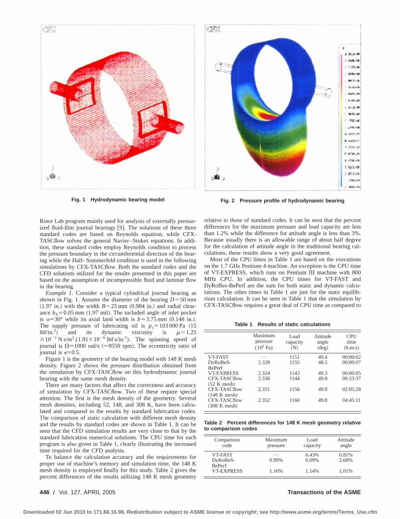
Rotor Lab program mainly used for analysis of externally pressur-ized fluid-film journal bearings@9#. The solutions of these threestandard codes are based on Reynolds equation, while CFX-TASCflow solves the general Navier–Stokes equations. In addi-tion, these standard codes employ Reynolds condition to processthe pressure boundary in the circumferential direction of the bear-ing while the Half- Sommerfeld condition is used in the followingsimulations by CFX-TASCflow. Both the standard codes and theCFD solutions utilized for the results presented in this paper arebased on the assumption of incompressible fluid and laminar flowin the bearing.

Example 1. Consider a typical cylindrical journal bearing asshown in Fig. 1. Assume the diameter of the bearingD550 mm~1.97 in.! with the width B525 mm ~0.984 in.! and radial clear-anceh050.05 mm~1.97 mil!. The included angle of inlet pocketis a530° while its axial land width isb53.75 mm ~0.148 in.!.The supply pressure of lubricating oil isps5103 000 Pa~15lbf/in.2! and its dynamic viscosity is m51.2531022 N s/m2 (1.8131026 lbf s/in.2). The spinning speed ofjournal is V51000 rad/s~'9550 rpm!. The eccentricity ratio ofjournal ise50.5.

Figure 1 is the geometry of the bearing model with 148 K meshdensity. Figure 2 shows the pressure distribution obtained fromthe simulation by CFX-TASCflow on this hydrodynamic journalbearing with the same mesh density.

There are many factors that affect the correctness and accuracyof simulation by CFX-TASCflow. Two of these require specialattention. The first is the mesh density of the geometry. Severalmesh densities, including 52, 148, and 308 K, have been calcu-lated and compared to the results by standard lubrication codes.The comparison of static calculation with different mesh densityand the results by standard codes are shown in Table 1. It can beseen that the CFD simulation results are very close to that by thestandard lubrication numerical solutions. The CPU time for eachprogram is also given in Table 1, clearly illustrating the increasedtime required for the CFD analysis.

To balance the calculation accuracy and the requirements forproper use of machine’s memory and simulation time, the 148 Kmesh density is employed finally for this study. Table 2 gives thepercent differences of the results utilizing 148 K mesh geometry

relative to those of standard codes. It can be seen that the percentdifferences for the maximum pressure and load capacity are lessthan 1.2% while the difference for attitude angle is less than 3%.Because usually there is an allowable range of about half degreefor the calculation of attitude angle in the traditional bearing cal-culations, these results show a very good agreement.

Most of the CPU times in Table 1 are based on the executionson the 1.7 GHz Pentium 4 machine. An exception is the CPU timeof VT-EXPRESS, which runs on Pentium III machine with 800MHz CPU. In addition, the CPU times for VT-FAST andDyRoBes-BePerf are the sum for both static and dynamic calcu-lations. The other times in Table 1 are just for the static equilib-rium calculation. It can be seen in Table 1 that the simulation byCFX-TASCflow requires a great deal of CPU time as compared to

Fig. 1 Hydrodynamic bearing model Fig. 2 Pressure profile of hydrodynamic bearing

Table 1 Results of static calculations

Maximumpressure(106 Pa)

Loadcapacity

~N!

Attitudeangle~deg!

CPUtime

~h:m:s!

VT-FAST ¯ 1151 49.4 00:00:02DyRoBeS-BePerf

2.328 1155 48.5 00:00:07

VT-EXPRESS 2.324 1143 49.3 00:00:05CFX-TASCflow~52 K mesh!

2.336 1144 49.8 00:33:37

CFX-TASCflow~148 K mesh!

2.351 1156 49.8 02:05:28

CFX-TASCflow~308 K mesh!

2.352 1160 49.8 04:45:11

Table 2 Percent differences for 148 K mesh geometry relativeto comparison codes

Comparisoncode

Maximumpressure

Loadcapacity

Attitudeangle

VT-FAST ¯ 0.43% 0.81%DyRoBeS-BePerf

0.99% 0.09% 2.68%

VT-EXPRESS 1.16% 1.14% 1.01%



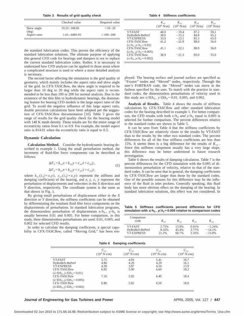
the standard lubrication codes. This proves the efficiency of thestandard lubrication solutions. The ultimate purpose of applyingthis general CFD code for bearings and dampers is not to replacethe current standard lubrication codes. Rather, it is necessary tounderstand how CFD analysis can be applied in those areas wherea complicated structure is used or where a more detailed analysisis necessary.

The second factor affecting the simulation is the grid quality ofgeometry, which mainly includes the aspect ratio and skew angleof the grid. In CFX-TASCflow, the skew angle is required to belarger than 10 deg to 20 deg while the aspect ratio is recom-mended to be less than 100 or 200 for normal analysis. Due to theexistence of the thin film in hydrodynamic bearings, the dominat-ing feature for bearing CFD models is the large aspect ratio of thegrid. To avoid the negative influence of this large aspect ratio,double precision calculations have been adopted per the sugges-tion of CFX-TASCflow documentation@10#. Table 3 gives therange of results for the grid quality check for the bearing modelwith 148 K mesh density. These results are for the entire range ofeccentricity ratios from 0.1 to 0.9. For example, the model aspectratio is 814.01 when the eccentricity ratio is equal to 0.5.

Dynamic Calculation

Calculation Method. Consider the hydrodynamic bearing de-scribed in example 1. Using the small perturbation method, theincrement of fluid-film force components can be described asfollows:

DFx5kxxx1kxyy1cxxx1cxyy,(1)

DFy5kyxx1kyyy1cyxx1cyyy,

where ki j ( i , j 5x,y), ci j ( i , j 5x,y) represent the stiffness anddamping coefficients of the bearing, andx, y, x, y represent theperturbation of displacements and velocities in theX direction andY direction, respectively. The coordinate system is the same asthat shown in Fig. 1.

By giving small perturbations of displacement either in theXdirection orY direction, the stiffness coefficients can be obtainedby differentiating the resultant fluid film force components on thedisplacements of perturbation. In standard lubrication programs,the dimensionless perturbation of displacementsx/h0 , y/h0 isusually between 0.01 and 0.005. For better comparison, in thisstudy, three dimensionless perturbations are used: 0.01, 0.005, and0.002 for selected CFD results.

In order to calculate the damping coefficients, a special capa-bility in CFX-TASCflow, called ‘‘Moving Grid,’’ has been em-

ployed. The bearing surface and journal surface are specified as‘‘Frozen’’ nodes and ‘‘Moved’’ nodes, respectively. Through theuser’s FORTRAN code, the ‘‘Moved’’ nodes can move in thefashion specified by the user. To match with the practice in stan-dard codes, the dimensionless perturbations of velocity used inthis study arex/Vh0 , y/Vh050.01, 0.005, and 0.002.

Analysis of Results. Table 4 shows the results of stiffnesscalculations by CFX-TASCflow and other standard lubricationcodes for the bearing described in example 1. For better compari-son, the CFD results with bothx/h0 and y/h0 equal to 0.005 isselected for further comparison. The percent differences relativeto the standard codes are shown in Table 5.

It can be seen from Table 4 that the stiffness coefficients byCFX-TASCflow are relatively closer to the results by VT-FASTthan to the results by the other two standard codes. The percentdifferences for all of the four stiffness coefficients are less than15%. It seems there is a big difference for the results ofKxy .Since this stiffness component usually has a very large slope,this difference may be better understood in future researchinvestigation.

Table 6 shows the results of damping calculation. Table 7 is thepercent differences for the CFD simulation with the 0.005 of di-mensionless perturbation of velocity, relative to that of the stan-dard codes. It can be seen that in general, the damping coefficientsby CFX-TASCflow are larger than those by the standard codes.One of the possible reasons for this difference may be the influ-ence of the fluid in inlet pockets. Generally speaking, this fluidbody has more obvious effect on the damping of the bearing. Instandard lubrication solutions, this effect was not considered. In

Table 3 Results of grid quality check

Checked value Required value

Skew angle~deg!

19.22–168.85 .10–20

Aspect ratio 1.01–4485.93 ,100–200

Table 4 Stiffness coefficients

Kxx

(106 N/m)Kxy

(106 N/m)Kyx

(106 N/m)Kyy

(106 N/m)

VT-FAST 40.0 219.4 87.2 59.1DyRoBeS-BePerf 38.0 215.2 84.8 65.2VT-EXPRESS 33.9 213.1 85.3 65.0CFX-TASCflow(x/h0 ,y/h050.01)

41.2 221.9 88.0 56.0

CFX-TASCflow(x/h0 ,y/h050.005)

41.1 222.1 88.0 56.0

CFX-TASCflow(x/h0 ,y/h050.002)

38.9 221.3 85.0 55.0

Table 5 Stiffness coefficients percent difference for CFDsimulation with x Õh 0 , y Õh 0Ä0.005 relative to comparison codes

Comparisoncode Kxx Kxy Kyx Kyy

VT-FAST 2.75% 13.9% 0.91% 25.24%DyRoBeS-BePerf 8.16% 45.4% 3.77% 214.1%VT-EXPRESS 21.2% 68.7% 3.16% 213.8%

Table 6 Damping coefficients

Cxx

(104 N s/m)Cxy

(104 N s/m)Cyx

(104 N s/m)Cyy

(104 N s/m)

VT-FAST 5.75 4.93 5.41 16.7DyRoBeS-BePerf 4.86 4.29 4.29 16.1VT-EXPRESS 4.38 3.87 4.50 15.9CFX-TASCflow( x/Vh0 ,y/Vh050.01)

6.92 5.90 6.60 18.2

CFX-TASCflow( x/Vh0 ,y/Vh050.005)

7.16 5.92 6.40 18.4

CFX-TASCflow( x/Vh0 ,y/Vh050.002)

6.86 5.82 6.50 18.0



addition, the differences in equation basis between two kinds ofsolutions may also be a cause. This will be a subject in futureresearch work.

Thermal AnalysisIn the thermal analysis, another capability in CFX-TASCflow,

‘‘Heat Transfer/Natural Convection,’’ is activated. The fluid prop-erty functions are introduced by employing the user’s FORTRANcode.

Example 2. Consider a cylindrical journal bearing as describedin example 1 and Fig. 1. Here the lubricating oil is ISO VG32~equivalent to DTE-LIGHT!.

Fluid Properties. Two cases are calculated in this thermalanalysis. The first case has an assumption of constant fluid prop-erties, which is typical in normal lubrication analysis. The secondcase assumes the fluid properties are a function of temperature,which is a more realistic simulation. These two cases are de-scribed in Table 8.

Simulation Results. In Fig. 3, the profiles of temperature andviscosity for case 2 at 0.5 of eccentricity ratio and 9550 rpm ofspeed are displayed. The performances of the bearing both forcase 1 and case 2 over the entire range of eccentricity ratios areshown in Fig. 4. For the purpose of comparison, the results byVT-EXPRESS are also displayed. Figure 5 is the maximum andaverage temperature curves of case 2.

Availability for Extended Thermal Analysis. The possibil-ity to conduct further thermal solutions where the model to beanalyzed includes both fluid film and solid elements, such as thebearing housing or journal, has been examined. This necessitatesthe ‘‘Conjugate Heat Transfer’’ capability in CFX-TASCflow. Fig-ures 6 and 7 display the results of an initial simulation which hasbeen conducted on a ‘‘long bearing’’ model. It can be seen that in

Table 7 Damping coefficients percent difference for CFDsimulation with x ÕVh 0 , y ÕVh 0Ä0.005 relative to comparisoncodes

Comparisoncode Cxx Cxy Cyx Cyy

VT-FAST 24.5% 20.1% 18.3% 10.2%DyRoBeS-BePerf 47.3% 38.0% 49.2% 14.3%VT-EXPRESS 63.4% 52.9% 42.2% 15.7%

Table 8 Two cases for thermal solutions

Feature Property values

Case 1 Constant properties ISO VG32 at50°C/122°F

Case 2 Function properties Functions for ISOVG32

Fig. 3 Temperature and viscosity distribution „case 2, 0.5 ofeccentricity ratio, 9550 rpm of speed …: „a… temperature, „b… dy-namic viscosity

Fig. 4 Bearing performances „5000 rpm of speed …: „a… load capacity, „b… maximum pressure „c… attitude angle, „d…mass flow



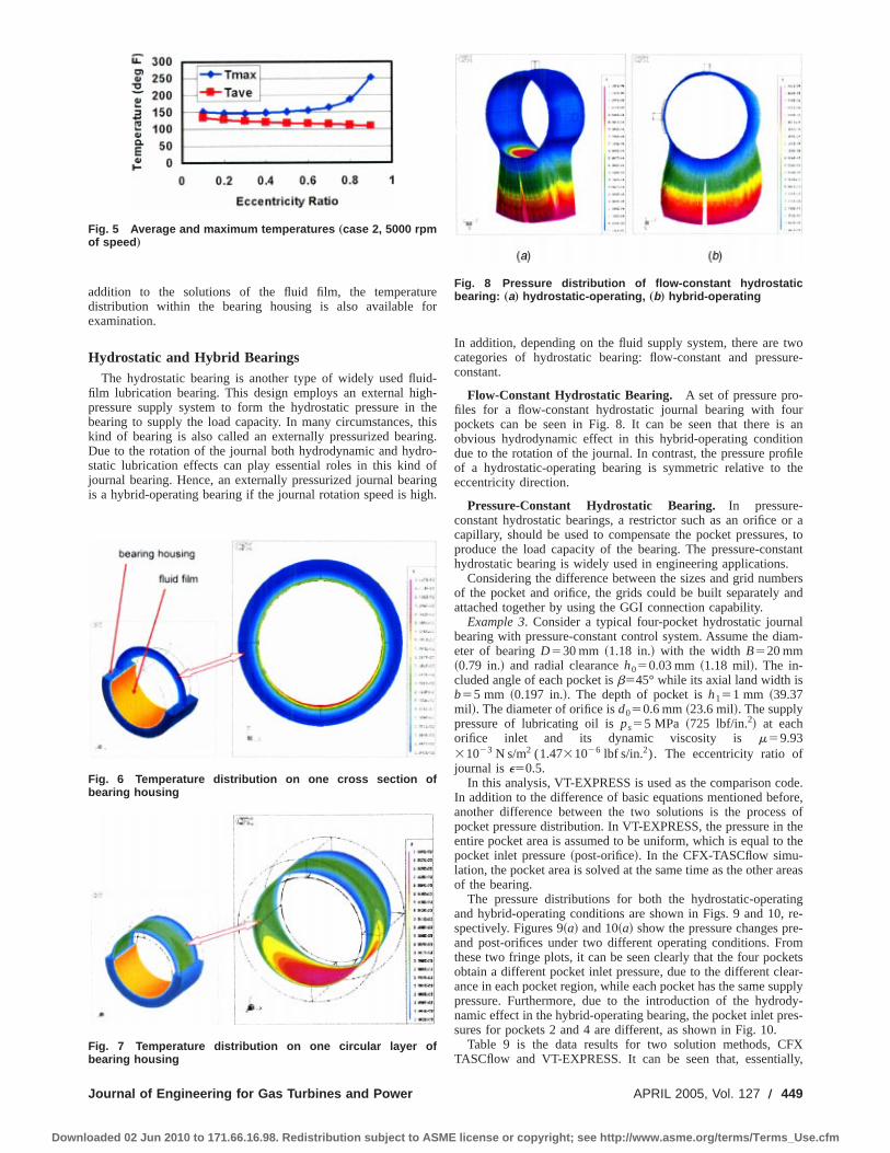
addition to the solutions of the fluid film, the temperaturedistribution within the bearing housing is also available forexamination.

Hydrostatic and Hybrid BearingsThe hydrostatic bearing is another type of widely used fluid-

film lubrication bearing. This design employs an external high-pressure supply system to form the hydrostatic pressure in thebearing to supply the load capacity. In many circumstances, thiskind of bearing is also called an externally pressurized bearing.Due to the rotation of the journal both hydrodynamic and hydro-static lubrication effects can play essential roles in this kind ofjournal bearing. Hence, an externally pressurized journal bearingis a hybrid-operating bearing if the journal rotation speed is high.

In addition, depending on the fluid supply system, there are twocategories of hydrostatic bearing: flow-constant and pressure-constant.

Flow-Constant Hydrostatic Bearing. A set of pressure pro-files for a flow-constant hydrostatic journal bearing with fourpockets can be seen in Fig. 8. It can be seen that there is anobvious hydrodynamic effect in this hybrid-operating conditiondue to the rotation of the journal. In contrast, the pressure profileof a hydrostatic-operating bearing is symmetric relative to theeccentricity direction.

Pressure-Constant Hydrostatic Bearing. In pressure-constant hydrostatic bearings, a restrictor such as an orifice or acapillary, should be used to compensate the pocket pressures, toproduce the load capacity of the bearing. The pressure-constanthydrostatic bearing is widely used in engineering applications.

Considering the difference between the sizes and grid numbersof the pocket and orifice, the grids could be built separately andattached together by using the GGI connection capability.

Example 3. Consider a typical four-pocket hydrostatic journalbearing with pressure-constant control system. Assume the diam-eter of bearingD530 mm ~1.18 in.! with the width B520 mm~0.79 in.! and radial clearanceh050.03 mm ~1.18 mil!. The in-cluded angle of each pocket isb545° while its axial land width isb55 mm ~0.197 in.!. The depth of pocket ish151 mm ~39.37mil!. The diameter of orifice isd050.6 mm~23.6 mil!. The supplypressure of lubricating oil isps55 MPa ~725 lbf/in.2! at eachorifice inlet and its dynamic viscosity is m59.9331023 N s/m2 (1.4731026 lbf s/in.2). The eccentricity ratio ofjournal ise50.5.

In this analysis, VT-EXPRESS is used as the comparison code.In addition to the difference of basic equations mentioned before,another difference between the two solutions is the process ofpocket pressure distribution. In VT-EXPRESS, the pressure in theentire pocket area is assumed to be uniform, which is equal to thepocket inlet pressure~post-orifice!. In the CFX-TASCflow simu-lation, the pocket area is solved at the same time as the other areasof the bearing.

The pressure distributions for both the hydrostatic-operatingand hybrid-operating conditions are shown in Figs. 9 and 10, re-spectively. Figures 9~a! and 10~a! show the pressure changes pre-and post-orifices under two different operating conditions. Fromthese two fringe plots, it can be seen clearly that the four pocketsobtain a different pocket inlet pressure, due to the different clear-ance in each pocket region, while each pocket has the same supplypressure. Furthermore, due to the introduction of the hydrody-namic effect in the hybrid-operating bearing, the pocket inlet pres-sures for pockets 2 and 4 are different, as shown in Fig. 10.

Table 9 is the data results for two solution methods, CFXTASCflow and VT-EXPRESS. It can be seen that, essentially,

Fig. 5 Average and maximum temperatures „case 2, 5000 rpmof speed …

Fig. 6 Temperature distribution on one cross section ofbearing housing

Fig. 7 Temperature distribution on one circular layer ofbearing housing

Fig. 8 Pressure distribution of flow-constant hydrostaticbearing: „a… hydrostatic-operating, „b… hybrid-operating



most of the results have a good agreement. The percent differ-ences for all of pocket inlet pressures~the mean values at pocketinlets in CFD solutions! are less than 2%. But, it seems the loadcapacity is an exception. The load capacities by CFX-TASCflowunder hydrostatic-operating and hybrid-operating conditions are

higher by 13.2% and 8.3%, respectively, than that by VT-EXPRESS. Generally speaking, under the hydrostatic-operatingcondition, the load capacity of the bearing is proportional to thedifference of pressures between the bottom and top pockets. Bychecking the pressure distribution in each pocket, it is found thatin the top pocket area~pocket 1! there is an obvious decrease inthe pressure field from the pocket inlet pressure~post-orifice pres-sure!. Figure 11 shows this phenomenon in hydrostatic-operatingcondition. It can be seen that the pressure values on most areas inthe top pocket are less than the pocket inlet pressure. This prob-ably is because the clearance of the bearing in this area increasesmore than the other areas after applying the eccentricity. Althoughthere is also a similar mechanism in the bottom pocket as well asthe other two pockets, the simulation results show this influence ismore evident right in the pocket opposite to the eccentricity direc-tion. In the VT-EXPRESS solution, the pressure in each pocketwas assumed to be the pocket inlet pressure. This phenomenoncan also be found in the hybrid-operating conditions.

Squeeze Film DamperA squeeze film damper~SFD! is a special kind of fluid-film

bearing, which exclusively makes use of only the squeeze effectresulting from the whirl of the journal to influence the vibration ofthe supported rotor systems. Squeeze film dampers are utilized in

Fig. 9 Pressure distribution under hydrostatic-operating con-dition: „a… pre- and post-orifice, „b… bearing surface

Fig. 10 Pressure distribution under hybrid-operating condi-tion „9550 rpm of speed …: „a… pre- and post-orifice, „b… bearingsurface

Table 9 Comparison of results by two solutions

Hydrostatic-operating Hybrid-Operating

CFX-TASCflow

VT-EXPRESS % diff

CFX-TASCflow

VT-EXPRESS % diff

#1 Pocketinletpressure~MPa!

2.657 2.650 0.3% 2.671 2.724 1.9%


4.104 4.165 1.5% 3.723 3.745 0.6%


4.959 4.975 0.3% 4.980 4.987 0.1%


4.104 4.165 1.5% 4.413 4.503 2.0%

Loadcapacity~N!

722.7 638.1 13.2% 727.0 670.9 8.3%

Attitudeangle~deg!

0 0 0% 23.4 25.7 8.9%

Flow rate~kg/s!

0.0324 0.0306 5.8% 0.0318 0.0304 4.6%

Fig. 11 Pressure decrease within pocket area in hydrostatic-operating bearing



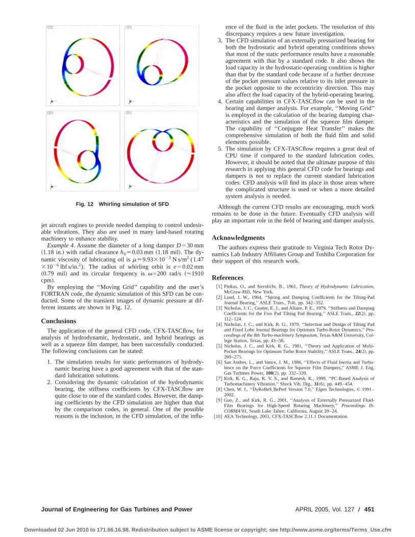
jet aircraft engines to provide needed damping to control undesir-able vibrations. They also are used in many land-based rotatingmachinery to enhance stability.

Example 4. Assume the diameter of a long damperD530 mm~1.18 in.! with radial clearanceh050.03 mm~1.18 mil!. The dy-namic viscosity of lubricating oil ism59.9331023 N s/m2 (1.4731026 lbf s/in.2). The radius of whirling orbit ise50.02 mm~0.79 mil! and its circular frequency isv5200 rad/s~'1910cpm!.

By employing the ‘‘Moving Grid’’ capability and the user’sFORTRAN code, the dynamic simulation of this SFD can be con-ducted. Some of the transient images of dynamic pressure at dif-ferent instants are shown in Fig. 12.

ConclusionsThe application of the general CFD code, CFX-TASCflow, for

analysis of hydrodynamic, hydrostatic, and hybrid bearings aswell as a squeeze film damper, has been successfully conducted.The following conclusions can be stated:

1. The simulation results for static performances of hydrody-namic bearing have a good agreement with that of the stan-dard lubrication solutions.

2. Considering the dynamic calculation of the hydrodynamicbearing, the stiffness coefficients by CFX-TASCflow arequite close to one of the standard codes. However, the damp-ing coefficients by the CFD simulation are higher than thatby the comparison codes, in general. One of the possiblereasons is the inclusion, in the CFD simulation, of the influ-

ence of the fluid in the inlet pockets. The resolution of thisdiscrepancy requires a new future investigation.

3. The CFD simulation of an externally pressurized bearing forboth the hydrostatic and hybrid operating conditions showsthat most of the static performance results have a reasonableagreement with that by a standard code. It also shows theload capacity in the hydrostatic-operating condition is higherthan that by the standard code because of a further decreaseof the pocket pressure values relative to its inlet pressure inthe pocket opposite to the eccentricity direction. This mayalso affect the load capacity of the hybrid-operating bearing.

4. Certain capabilities in CFX-TASCflow can be used in thebearing and damper analysis. For example, ‘‘Moving Grid’’is employed in the calculation of the bearing damping char-acteristics and the simulation of the squeeze film damper.The capability of ‘‘Conjugate Heat Transfer’’ makes thecomprehensive simulation of both the fluid film and solidelements possible.

5. The simulation by CFX-TASCflow requires a great deal ofCPU time if compared to the standard lubrication codes.However, it should be noted that the ultimate purpose of thisresearch in applying this general CFD code for bearings anddampers is not to replace the current standard lubricationcodes. CFD analysis will find its place in those areas wherethe complicated structure is used or when a more detailedsystem analysis is needed.

Although the current CFD results are encouraging, much workremains to be done in the future. Eventually CFD analysis willplay an important role in the field of bearing and damper analysis.

AcknowledgmentsThe authors express their gratitude to Virginia Tech Rotor Dy-

namics Lab Industry Affiliates Group and Toshiba Corporation fortheir support of this research work.

References@1# Pinkus, O., and Sternlicht, B., 1961,Theory of Hydrodynamic Lubrication,

McGraw-Hill, New York.@2# Lund, J. W., 1964, ‘‘Spring and Damping Coefficients for the Tilting-Pad

Journal Bearing,’’ ASLE Trans.,7~4!, pp. 342–352.@3# Nicholas, J. C., Gunter, E. J., and Allaire, P. E., 1979, ‘‘Stiffness and Damping

Coefficients for the Five Pad Tilting Pad Bearing,’’ ASLE Trans.,22~2!, pp.112–124.

@4# Nicholas, J. C., and Kirk, R. G., 1979, ‘‘Selection and Design of Tilting Padand Fixed Lobe Journal Bearings for Optimum Turbo-Rotor Dynamics,’’Pro-ceedings of the 8th Turbo-machinery Symposium, Texas A&M University, Col-lege Station, Texas, pp. 43–58.

@5# Nicholas, J. C., and Kirk, R. G., 1981, ‘‘Theory and Application of Multi-Pocket Bearings for Optimum Turbo Rotor Stability,’’ ASLE Trans.,24~2!, pp.269–275.

@6# San Andres, L., and Vance, J. M., 1986, ‘‘Effects of Fluid Inertia and Turbu-lence on the Force Coefficients for Squeeze Film Dampers,’’ ASME J. Eng.Gas Turbines Power,108~2!, pp. 332–339.

@7# Kirk, R. G., Raju, K. V. S., and Ramesh, K., 1999, ‘‘PC-Based Analysis ofTurbomachinery Vibration,’’ Shock Vib. Dig.,31~6!, pp. 449–454.

@8# Chen, W. J., ‘‘DyRoBeSIBePerf Version 7.0,’’ Eigen Technologies, © 1991–2002.

@9# Guo, Z., and Kirk, R. G., 2001, ‘‘Analysis of Externally Pressurized Fluid-Film Bearings for High-Speed Rotating Machinery,’’Proceedings IS-CORMA’01, South Lake Tahoe, California, August 20–24.

@10# AEA Technology, 2001, CFX-TASCflow 2.11.1 Documentation.

Fig. 12 Whirling simulation of SFD



journal of engineering for gas turbines and power 2005.vol.127.n2

Documents

practical combustor2003gt

gas turbine aeroengine

mullendergas turbines

mw gas turbine engine

combustion technologiesk

address changes

changes of address

personal use