journal of economic dynamics · 138 a. consiglio, s.a. zenios / journal of economic dynamics &...
TRANSCRIPT

Journal of Economic Dynamics & Control 88 (2018) 137–155
Contents lists available at ScienceDirect
Journal of Economic Dynamics & Control
journal homepage: www.elsevier.com/locate/jedc
Pricing and hedging GDP-linked bonds in incomplete markets
Andrea Consiglio
a , Stavros A. Zenios b , c , d , ∗
a University of Palermo, Palermo, Italy b University of Cyprus, Nicosia, Cyprus c Norwegian School of Economics, Norway d The Wharton Financial Institutions Center, The Wharton School, University of Pennsylvania, PA, USA
a r t i c l e i n f o
Article history:
Received 6 June 2017
Revised 6 September 2017
Accepted 2 January 2018
Available online 5 January 2018
Keywords:
Contingent bonds
Debt restructuring
Asset pricing
Incomplete markets
Risk premium
Stochastic programming
Super-replication
a b s t r a c t
We model the super-replication of payoffs linked to a country’s GDP as a stochastic linear
program on a discrete time and state-space scenario tree to price GDP-linked bonds. As a
byproduct of the model we obtain a hedging portfolio. Using linear programming duality
we compute also the risk premium. The model applies to coupon-indexed and principal-
indexed bonds, and allows the analysis of bonds with different design parameters (coupon,
target GDP growth rate, and maturity). We calibrate for UK and US instruments, and carry
out sensitivity analysis of prices and risk premia to the risk factors and bond design pa-
rameters. We also compare coupon-indexed and principal-indexed bonds.
Further results with calibrated instruments for Germany, Italy and South Africa shed
light on a policy question, whether the risk premia of these bonds make them benefi-
cial for sovereigns. Our findings affirm that designs are possible for both coupon-indexed
and principal-indexed bonds that can benefit a sovereign, with an advantage for coupon-
indexed bonds. This finding is robust, but a nuanced reading is needed due to the many
inter-related risk factors and design parameters that affect prices and premia.
© 2018 Published by Elsevier B.V.
1. Introduction
An old idea for sovereign contingent debt was revived at the G20 meeting in Chengdu, China, in July 2016. There
are theoretical arguments in favor of contingent debt for sovereigns, originating in the works of Krugman (1988) and
Froot et al. (1989) , and the International Monetary Fund (IMF) was asked to analyze “technicalities, opportunities, and chal-
lenges of state-contingent debt instruments, including GDP-linked bonds”1 . Within a year IMF submitted a comprehensive
report ( IMF, 2017a; 2017b ). In this paper we contribute a model for pricing and hedging GDP-linked bonds, and use it to
estimate risk premia and compare two competing bond designs.
GDP-linked bonds make debt payments contingent on a country’s GDP, thereby ensuring that debt can always be ser-
viced. Linking instruments to GDP growth was first suggested during the debt crisis of the 1980s in the context of debt re-
structuring. Concerned about a country’s growth prospects in the aftermath of the crisis, creditors and debtor governments
sought instruments for risk sharing to increase debt resilience to macroeconomic shocks. A brief history of these instruments
is given in Borensztein and Mauro (2004) . Early attention was restricted to warrants that provide additional payments if a
favorable event occurs, such as an increase in prices of commodities (e.g., oil, copper). Such warrants (also called value recov-
∗ Corresponding author.
E-mail addresses: [email protected] (A. Consiglio), [email protected] (S.A. Zenios). 1 Paragraph 11 of Communiqué G20 Finance Ministers and Central Bank Governors Meeting, G20 Web Site, 28 July 2016, available at http://www.g20.
utoronto.ca/2016/160724-finance.html , last accessed February 14, 2018.
https://doi.org/10.1016/j.jedc.2018.01.001
0165-1889/© 2018 Published by Elsevier B.V.
138 A. Consiglio, S.A. Zenios / Journal of Economic Dynamics & Control 88 (2018) 137–155
ery rights ) were offered to investors as part of the Brady restructuring process for Mexico, Nigeria, Uruguay, and Venezuela.
Value recovery rights indexed to GDP growth were also included in debt instruments of Costa Rica and Bosnia and Herze-
govina ( Borensztein et al., 2004 ), and Bulgaria issued indexed debt with a call option in 1994. More recent examples are
Argentina in 2005, Greece in 2012, and Ukraine in 2015. The Argentinean GDP-linked warrants received attention in the
academic literature and ( Datz, 2009; Guzman, 2016 ) document significant gains for investors in these instruments, which,
in turn, implies smaller haircuts for investors who accepted these instruments as part of a debt restructuring deal. In these
early instruments sovereigns are funded mostly by plain vanilla bonds, and detachable linked instruments served as sweet-
eners in debt restructuring. The G20 interest is in cash instruments that pay differentially both on the upside and downside,
depending on growth. It is these instruments we call GDP-linked bonds. The debate on benefits from potential issuance by
sovereigns is ongoing, and it is for these instruments that we develop pricing and hedging models, and estimate risk premia.
GDP-linked bonds provide insurance from negative growth shocks ( Froot et al., 1989 ), provide long-term investors an
instrument to hedge income risks and invest in the “wealth of nations” ( Shiller, 1993 ), allow governments to smooth taxation
over the economic cycle ( Barro, 2003 ), and reduce reliance on large-scale official sector support programs, thereby improving
the functioning of the international financial system ( Barr et al., 2014 ). Concerns that countries would manipulate GDP, or,
in extremis , suppress growth to avoid debt repayment, were countered by proposals to link bond payments to exogenous
factors that affect a country’s macroeconomic conditions, such as commodity prices ( Caballero and Panageas, 2008; Froot
et al., 1989; Krugman, 1988 ). The earlier GDP-linked warrants pay only on the upside, so they are distant relatives to the
new instruments, and ( Borensztein and Mauro, 2004; Obstfeld and Peri, 1998 ) suggest that governments reduce idiosyncratic
GDP risks by issuing such warrants.
Potential pitfalls in emitting GDP-linked bonds —moral hazard, imprecise, erroneous and/or manipulated statistics,
call options— and ways to avoid them are summarized in Borensztein and Mauro (2004) , Brooke et al. (2013) and
Benford et al. (2016) . These papers argue in favor of GDP-linked bonds, although ( Brooke et al., 2013 ) also argue for a
complement to GDP-linked bonds in the form of sovereign contingent convertible debt. This suggestion was advanced in the
S-CoCo instrument of Consiglio and Zenios (2015) who propose a design with contingent payment standstill and develop
pricing and risk management models ( Consiglio et al., 2016b ), noting that this instruments preserves the features of debt,
whereas GDP-linked bonds are equity-like instruments.
Neither GDP-linked bonds nor GDP per se are currently traded. Hence, the markets are incomplete and there is a dearth
of pricing and hedging models for these instruments. The lack of a pricing model is not necessarily an obstacle to issuing
GDP-linked bonds —stocks and options were traded before Black-Scholes/Merton developed their formulas— but availability
of such models will encourage the development of a market ( Borensztein et al., 2004; Griffith-Jones and Sharma, 2006 ).
Bank of England authors ( Benford et al., 2016 ) adopt a Darwinian stance towards the development of GDP-linked markets
by suggesting the commission of a set of “rival pricing models”. The primary contribution of our paper is a model for pricing
GDP-linked bonds in incomplete markets, using stochastic linear programming to compute a super-replicating portfolio. As
a byproduct of the model we obtain a hedging portfolio for investors in these novel instruments, and using linear program-
ming duality we compute risk premia for bonds of different designs.
Sovereigns will benefit from GDP-linked bonds if they are not too expensive, and several researchers are asking “At what
premium do the benefits of GDP-linked debt payments outweigh the burden of issuing more expensive debt?”. We use
the pricing model to calculate risk premia and answer the policy question whether GDP-linked bonds are beneficial for
sovereigns.
In the computational part of the paper we apply the model to price instruments for UK and US, and study the sensitivity
of prices and risk premia to the risk factors and bond design parameters. We also estimate risk premia for different GDP-
linked bond designs, including designs for Germany, Italy and South Africa. Comparing with premium thresholds from the
literature we draw conclusions on designs that are beneficial for sovereigns. The model is also used to compare two bond
designs that compete for attention in the current debate, namely coupon-indexed and principal-indexed bonds, called floaters
and linkers , respectively, in the report by IMF (2017a) .
The paper is organized as follows. Section 2 reviews literature for pricing GDP-linked bonds and pricing in incomplete
markets, develops the model for pricing and hedging GDP-linked bonds, and shows how to estimate the risk premium.
Section 3 describes the calibration and reports numerical results. Section 4 concludes.
2. The pricing model
The market for GDP-linked bonds is incomplete in the sense defined in Pliska (1997) . Not every GDP contingent claim
can be generated by some trading strategy using market instruments. There are many source of market incompleteness, the
most significant for the present study being the lack of instruments trading in GDP. Even when a suitable proxy is identified
—such as, for instance, the use of copper prices for the Chilean economy ( Caballero and Panageas, 2008; Froot et al., 1989;
Krugman, 1988 )— other sources of market incompleteness remain, such as jumps in the underlying stochastic process due
to exogenous shocks to the economy or market crashes for the proxy, and heteroskedasticity of the GDP process. (Other
sources of market incompleteness, such as frictions arising from transactions costs and the use of discrete hedging, are not
unique to the GDP bond markets.)
Assuming market completeness, Kruse et al. (2005) develop a Black-Scholes type pricing model using a single-factor
stochastic model when GDP follows a log-normal distribution and interest rates are deterministic, and they use it to
A. Consiglio, S.A. Zenios / Journal of Economic Dynamics & Control 88 (2018) 137–155 139
estimate returns on linked and plain bonds for Indonesia and Venezuela. Miyajima (2006) develops pricing models for
GDP-linked warrants using a Brownian motion for the GDP and Monte Carlo simulations on foreign currency and infla-
tion conditions, and studies the sensitivity of prices to exchange rate and GDP shocks. This model assumes risk neutral
investors. Kamstra and Shiller (2009) price their version of GDP-linked bond (the “trill”) using a fundamental valuation
dividend-discounting method to estimate prices and yields for GDP-linked bonds and, applying portfolio diversification, they
conclude that long-term investors will hold a portfolio of 28% bonds, 38% S&P500 and 34% linked bonds. This model needs
an exogenously determined risk premium and the authors assume a value 350bp, which is the risk premium used to dis-
count risky equities. Bowman and Naylor (2016) use CAPM (and downside-CAPM) to obtain a range of premia for G20
countries and contribute to the policy debate on the benefits of these instruments (although their empirical findings do not
lead to clear conclusions). These market-based premia estimates could be used in a model such as the one of Kamstra and
Shiller (2009) to price the instruments.
Our methodological approach is distinct from these earlier works and allows us to overcome their limiting assumptions.
We account for the fact that markets are incomplete, and estimate prices and premia that are internally consistent and
externally consistent with market data. The model does not need assumptions on investor risk aversion ( Barr et al., 2014 ) or
exogenous estimation of a premium ( Kamstra and Shiller, 2009 ), and, uniquely in the literature, provides a hedging portfolio
for GDP-linked bond investors.
In incomplete markets a unique price for a contingent claim may not exist, but the absence of arbitrage specifies a price
range. Following King (2002) we use stochastic linear programming to compute a super-replication strategy on a discrete
market model. A positive optimal objective value for the stochastic program identifies an arbitrage strategy that begins with
a zero value portfolio, makes self-financing trades at each time step, has non-negative terminal values in all scenarios, and
has positive expected value at maturity. The optimal value of the stochastic program is the price of the contingent claim
that must be paid up front so that the net value of the hedging portfolio and the contingent claim payoff is zero, thus
precluding arbitrage. The least cost of super-replication is the seller’s price, whereas the greatest amount a buyer could
pay for the contingent claim without negative terminal wealth is the buyer’s price. The theory for obtaining price bounds
on contingent claims in incomplete markets is developed in King et al. (2005) . In this section we formulate a stochastic
programming model for computing bid and ask prices for GDP-linked bonds.
The models we develop can be applied to other derivatives linked to macroeconomic indicators. For instance, ( Baron and
Lange, 2007 , pp. 36–37) report that Goldman Sachs and Deutsche Bank completed in September 2002 parimutuel auctions
of options on the US Bureau of Labor Statistics release of US Non-farm Payroll data, and in April 2003 they hosted auctions
for 3- and 6-month options on the European Harmonized Index of Consumer Prices. Our work shows that we can price such
derivatives in the absence of a complete market, even if the prices are estimated within a bid-ask spread.
There are two types of GDP-linked bonds and we price both:
Coupon-indexed bonds link the coupon to GDP growth ( Borensztein and Mauro, 2004 ) by
c t = max [ c 0 + (g t − g ) , 0 ] , (1)
where g t is the real growth rate, g is a contractually specified target growth rate, and c 0 is the baseline coupon rate.
If growth exceeds the target, the coupon will increase from the baseline, otherwise coupon payments decrease, with
a floor at zero. These instruments are called floaters in IMF (2017a) .
Principal-indexed bonds pay principal at maturity ( Kamstra and Shiller, 2009 ),
B t = B 0 Y t
Y 0 . (2)
B 0 is the amount issued, typically set at 100, and Y 0 , Y t are the nominal GDP values at the issuing date and t , respec-
tively. Coupon payments satisfy (1 + c 0 ) B t = (1 + c 0 ) B 0 Y t Y 0
, so the effective coupon rate per 100 units of debt is given
by
1 + c t = (1 + c 0 ) Y t
Y 0 . (3)
These instruments are called linkers in IMF (2017a) .
There are several variations of these two instruments ( Kruse et al., 2005 ), and all can be priced using our model. Spec-
ifications of an instrument are given by some functions c t = �(g t ) or c t = �(Y t ) , and these functions are an input to the
pricing model. For instance, the Greek GDP-linked security, issued as part of debt restructuring in 2012, stipulates coupons
equal to 1.5 times the excess GDP growth over a target g = 2 . 9% until 2020, and 2% afterwards.
2.1. Model preliminaries
We assume that the time horizon of the investor consists of a finite set of decision stages T = { 0 , 1 , 2 , . . . , T } , and that
the market consists of J + 1 securities with prices S t =
(S 0 t , S
1 t , . . . , S
J t
)at each t ∈ T . Without loss of generality we use S 0 t for

140 A. Consiglio, S.A. Zenios / Journal of Economic Dynamics & Control 88 (2018) 137–155
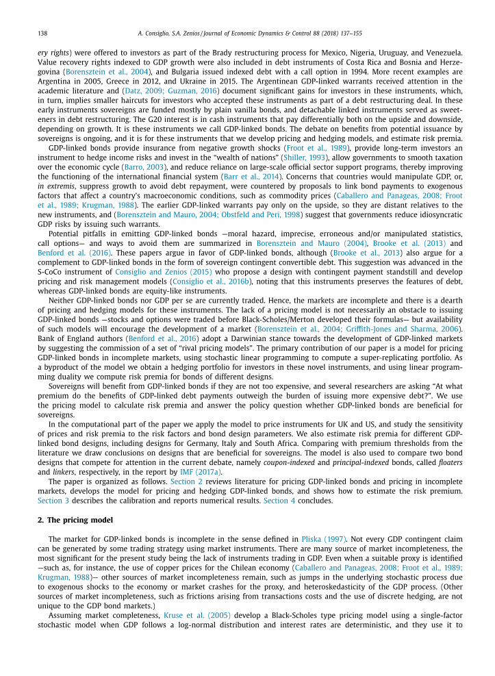
Fig. 1. A finite filtration (left panel) and its associated scenario tree (right panel).
the price at time t of 1 € invested in the money market at time 0, and express security prices in terms of the numéraire
βt = 1 /S 0 t . The discounted price process
Z t =
S t
S 0 t
= βt S t (4)
denotes prices relative to the numéraire. Expressing prices relative to a numéraire, or as a discounted price process, is not
done only to account for time value. Under certain hypotheses it can be proved that the stochastic process Z t is a martingale
with respect to a measure Q . In continuous time, this property is expressed by
Z t = E Q [ Z T |F t ] , (5)
where E is the expectation operator and F t is a filtration.
For discrete time and discrete probability space � = { ω 1 , ω 2 , . . . , ω L } , the evolution of the risky asset price S t can be
represented using scenario trees . A scenario tree is a set of states, and interconnecting links denoting possible transitions
between states. In particular, at each non-final state corresponds one, and only one, ancestor state a ( n ), and a non-empty
set of child states C(n ) . In this structure, the filtration F t is a partition of � into sets A t , with A t ⊆ A t+1 , with one-to-one
correspondence between A t and the set of states of the tree N t , see Fig. 1 . The martingale property on a tree is a conditional
expectation with respect to the set of states at t :
Z t = E Q [ Z T |N t ] . (6)
Following King (2002) , we assume that the random process S t is measurable with respect to N t , meaning that S n is the
value taken by S t at each state n ∈ N t . If we denote by K(n ) the set of states m ∈ N T that can be reached from n ( K(n ) ⊆ N T ),
eq. (6) becomes
Z n =
∑
m ∈K(n )
q m
q n Z m
. (7)
Note that for Z 0 , q 0 = 1 and K(0) = N T . The set of weights q n > 0 attached to each terminal state n ∈ N T form the risk neutral
probability distribution Q . Q is equivalent to the objective probability measure P —in the sense that P and Q both agree on
the set of events with null probability— identified by the set of weights p n > 0, n ∈ N T , with
∑
n ∈N T p n =
∑
n ∈N T q n = 1 . (8)
The existence of a risk neutral measure Q ensures that arbitrage is ruled out, and Q is unique in complete markets.
2.2. The super-replication pricing model
Let us assume that we are supplied with a scenario tree endowed with both risk neutral Q and objective P probability
measures, such as the one of Consiglio et al. (2016a) , and let S 1 denote the GDP level of a given country. If the market is
complete, then we can price any claim with payoffs contingent on the GDP through some function �( S 1 ), by discounting its
expected payoff under Q . This price, however, would be incorrect for GDP-linked bonds. The underlying assumption is that
the payoff �(S 1 n ) is attainable by means of a self-financing portfolio, which implies that it is possible to trade the GDP, or
A. Consiglio, S.A. Zenios / Journal of Economic Dynamics & Control 88 (2018) 137–155 141
that there exists an asset (e.g., a future on GDP) that reproduces GDP dynamics. If such an asset does not exist, then the
price of the GDP contingent claim, which is the cost of the replicating portfolio, can not be obtained. In particular, either
the buyer or the seller will incur higher costs. The seller asks a price equal to the lowest cost for hedging the payoff stream
with instruments not perfectly replicating the GDP dynamics. Similarly, the buyer bids at a price that is the highest cost of
a portfolio producing at least the same payoff as the GDP contingent claim. The equilibrium price lies between the buyer
and seller prices, and the difference between the two is the bid-ask spread .
A way to model buyer and seller behavior is to select a portfolio that super-replicates the payoff. The lower, in absolute
value, the correlation of assets with the GDP, the higher will be the cost (for buyer and seller) to hedge the cashflows,
and the wider the bid-ask spread. Following King (2002) and Consiglio and De Giovanni (2010) we formulate the super-
replication problem as a stochastic program on the scenario tree. Seller’s price V is the minimum amount that an issuer
asks for selling the cashflows �( S 1 ) without risk of negative terminal wealth, and is the solution of:
Minimize V,θ
V (9)
s.t.
Z 0 · θ0 = V, (10)
Z n · (θn − θa (n ) ) = −βn �(S 1 n ) , n ∈ N t , t ≥ 1 , (11)
Z n · θn ≥ 0 , n ∈ N T , (12)
θ1 n = 0 , n ∈ N , (13)
where θn = (θ1 n , θ
2 n , . . . , θ
J n ) is the hedging portfolio at state n . Constraints (13) take into account the non-tradeability of GDP
( S 1 n ) by fixing the corresponding weights ( θ1 n ) to zero.
The super-replication model for the buyer’s price computes the maximum amount the buyer is willing to bid to purchase
�( S 1 ) without risk of falling short at maturity:
Maximize V,θ
V (14)
s.t.
Z 0 · θ0 = −V, (15)
Z n · (θn − θa (n ) ) = βn �(S 1 n ) , n ∈ N t , t ≥ 1 , (16)
Z n · θn ≥ 0 , n ∈ N T , (17)
θ1 n = 0 , n ∈ N . (18)
In complete markets, the bid and ask prices coincide, and the pricing mechanism simply reduces to discounting the expected
cashflows with respect to Q .
It is instructive to model the contingent claim price as the dual of (9) –(13) . The price will be the same, but the dual also
provides the risk neutral measure Q for an incomplete market, which is used to estimate risk premia in Section 2.3 . Since
risk premia are endogenous, the model is internally consistent.
Following King (2002) , the dual problem of (9) –(13) is:
Maximize q
T ∑
t=1
∑
n ∈N t q n βn �(S 1 n ) (19)
s.t.
q n ≥ 0 , n ∈ N T , (20)
q 0 = 1 , (21)
∑
m ∈C(n )
q m
Z j m
= q n Z j n , j � = 1 , n ∈ N t , t = 0 , 1 , . . . , T − 1 . (22)
Unlike King (2002) , we introduce the martingale measure q n for the discounted process Z n . Constraints (22) ensure that
q n is a martingale measure, cf. Eq. (7) . To take into account the non-tradeability of GDP, martingale equations are defined
for all risk factors except Z 1 n . q n is associated with the incomplete market price of the GDP-linked bond, and, as explained
next, there is a close relation between risk neutral probabilities and the stochastic discount factor.
142 A. Consiglio, S.A. Zenios / Journal of Economic Dynamics & Control 88 (2018) 137–155
2.3. Estimating the risk premium
To assess the merits of GDP-linked bonds we need to examine two counteracting effects. The decrease in default risk of
GDP-linked financed sovereigns lowers risk premia, whereas the systematic risk of bonds linked to a volatile GDP commands
a premium. Several researchers estimate a risk premium threshold that makes these instruments attractive for sovereigns.
Barr et al. (2014) study the effect of GDP-linked bonds on the maximum sustainable level of debt and the probability of
default of a sovereign. Modeling the cost of the risk premium and the lowered default probabilities of GDP-linked bonds
they conclude that there are welfare gains for risk premium lower than 350bp. (Recall that risk premia are negative and in
the text we refer to absolute values.) Blanchard et al. (2016) simulate the effects of plain bonds and GDP-linked bonds on
default probabilities and find that GDP-linked bonds dominate when the risk premium is 100bp, but at 200bp plain bonds
are favored. (Their threshold depends on the original indebtedness.) Benford et al. (2016) report similar findings. The take
from these papers is that for risk premia above 350bp the GDP-linked bonds are too expensive. 2 Values in the range 100bp–
350bp (250bp for more conservative estimates) indicate that GDP-linked bonds benefit sovereigns. For premia lower than
100bp the probability of insolvency is reduced significantly by issuing GDP-linked debt to compensate for the systematic
risk of GDP volatility. These results serve as thresholds when assessing the viability of financing sovereigns with GDP-linked
bonds. We use 250bp as a tight threshold and 350bp as a relaxed threshold. For advanced economies, where default is
a neglected risk ( Gennaioli et al., 2012 ) and sovereigns would be unwilling to pay a high premium for issuing GDP-linked
bonds, we use tighter thresholds in the range 100bp ( Blanchard et al., 2016 ) to 50bp which is about the premium of U.S.
inflation-linked treasury bonds ( IMF, 2017a ).
The studies cited above do not estimate what the premium will be but what it should be for the issuing sovereign to
benefit and be willing to pay it. Our interest is to estimate the risk premium and compare it to the thresholds. To do so
requires that several risk factors are disentangled. Borensztein et al. (2004) and Griffith-Jones and Sharma (2006) identify
the risk factors which are summarized by Blanchard et al. (2016) as follows:
Novelty premium for buying a new and unfamiliar investment product.
Liquidity premium for converting the asset into cash at fair market value in thin markets.
Default premium for the risk that the debtor will not make the required repayments. (This premium is positive if GDP-
linked bonds make debt more sustainable.)
Growth risk premium for exposure to a country’s economic growth uncertainty.
The first two risk premia are transitory. Novelty and liquidity premia decline as the markets deepen. For instance,
Costa et al. (2008) find the novelty premium on Argentina’s GDP-linked warrants declined by about 600bp during the first
18 months after issuance. It is hard to model these premia and the (limited) research on pricing GDP-linked bonds focuses
on estimating the growth risk premium. We show how to obtain the risk premium from our model.
Consider a stochastic payoff x linked to the GDP (the precise form of the link x = �(S 1 ) is not important) with price P 0
obtained from ( Cochrane, 2005 , Eq. (1.9)):
P 0 =
E P (x )
1 + r f + cov (m, x ) . (23)
r f is the risk free rate of return and m is the stochastic discount factor, with 1 = E P ((1 + r f ) m ) . The first term on the right
is the discounted expected value under the objective probability measure and the second term is a risk adjustment. Assets
with payoffs negatively correlated to the discount factor have lower prices and, therefore, have higher excess return over
the risk free rate. Debt with payoffs negatively correlated to the discount factor will be more expensive.
The interpretation of the second term as a risk premium is better understood if, following ( Cochrane, 2005 , Eq. (1.10)),
we write
P 0 =
E P (x )
1 + r f +
cov (βU
′ (C t+1 ) , x t+1 )
U
′ (C t ) , (24)
where β is the subjective discount factor capturing impatience, U(·) the investor utility function, and C t , C t+1 the consump-
tion at t and t + 1 . The second term is negative if the payoff covaries negatively with the marginal utility, and since marginal
utility declines as consumption rises, the term is negative if payoff covaries positively with consumption. This is key to un-
derstanding the risk premium: if payoff is correlated with consumption it makes consumption more volatile, and investors
demand a price discount to buy the asset. Equivalently, investors expect higher return for holding the asset.
The risk premium can be obtained from our pricing model. The price P 0 is computed under the risk neutral probability
measure ( Cochrane, 2005 , Section 3.2) by
P 0 =
E Q (x )
1 + r f . (25)
2 In a recent presentation, J.D. Ostry and J.I. Kim of the IMF put the premium in the range 153bp–260bp for low and high growth uncertainty countries,
respectively, which is somewhat lower than previous studies.
A. Consiglio, S.A. Zenios / Journal of Economic Dynamics & Control 88 (2018) 137–155 143
Table 1
Execution times for tree calibration and solution of the pricing model. The size of the stochastic program
grows with bond maturity. Better memory management can reduce tree building times, even though for
longer maturities coarser discretization might be needed.
Maturity (years) Tree building
time (h:m:s)
Pricing model stochastic program size Pricing model solution
time (h:m:s) Equations Variables Nonzeros
2 0:00:01 72 63 560 0:0 0:0 0
3 0:00:02 584 511 4,592 0:00:01
4 0:00:13 4,680 4,095 36,848 0:00:01
5 0:07:11 37,448 32,767 294,896 0:00:09
6 6:52:10 299,592 262,143 2,359,280 0:07:23
Combining (23) and (25) we write the risk premium as
cov (m, x ) =
E Q (x )
1 + r f − E P ( x )
1 + r f . (26)
The first term on the right is the price of a risk averse investor, calculated from our pricing model by discounting the payoff
under the risk neutral measure Q . The second term is the price of a risk neutral investor, computed by discounting under
the objective measure P . 3 Alternatively, we can calculate the covariance of the payoffs with the discount factor that is also
obtained from the calibrated scenario tree by m =
q p(1+ r f ) .
It is worth repeating that the risk premium calculation is endogenous to the model, so that prices and premia are in-
ternally consistent. The model does not need any assumptions on investor risk aversion ( Barr et al., 2014 ), or exogenous
estimation of a premium ( Kamstra and Shiller, 2009 ). Market information is conveyed through the calibrated tree under
only an assumption of absence of arbitrage, and is used to estimate both prices and risk premia.
3. Numerical results
We calibrate the models for GDP-linked bonds for UK and US in year 2013, and use them to (i) study the effect of risk
factors and bond design choices on the prices of different coupon-indexed bonds, (iii) estimate risk premia, and (iii) compare
the coupon-indexed and principal-indexed bonds. We also estimate the risk premia for bond designs for Germany, Italy and
South Africa and compare them with appropriate thresholds from the literature to shed light on the policy question whether
the risk premia of these bonds make them beneficial for sovereigns.
We calibrate the arbitrage-free tree of Consiglio et al. (2016a) for each country using asset returns from the Dimson–
Marsh–Staunton Global Returns Data ( Dimson et al., 2002 ) and GDP data from Schularick and Taylor (2012) . For each coun-
try we use as traded assets its own T-bills, bonds and equity indices, plus the World bills, bonds and equity indices in
local currency. The database uses US T-bills as the World bills index, so for the US model we use the three US assets
plus the World (ex-US) bonds and equity indices. For risk free rates we use the yield curve on treasury bonds from Bank
of England and US Department of Treasury of December 31, 2013, ECB data for Germany and Italy of January 2013, and
South Africa Reserve Bank data of 2013. Means, standard deviations and correlations of the time series are estimated for
the time windows 1983–2013, 1993–2013, and 2003–2013, see Appendix A . We also use IMF projections for GDP growth for
the UK (1.5%) and the US (2.3%) with the 2003–2013 calibrated asset data. Data used to estimate moments are in nominal
values.
Pricing proceeds in two steps. First, a tree is calibrated on estimated market moments, and, second, the stochastic pro-
grams are solved to determine seller and buyer prices. The stochastic program is implemented in the algebraic modeling
language GAMS ( GAMS, 2016 ) and optimized using solver CPLEX . To illustrate the computational demands of the procedure
we summarize in Table 1 the total execution time of both steps, and the sizes and solution times of the stochastic program.
All models are solved on a machine with an Intel Xeon processor with 32 Gbytes RAM. The most time consuming part is for
tree building, however once a tree is built it is used repeatedly to price multiple instruments and calculate risk premia. The
large execution time is due to the need to store the tree in a database for the extensive numerical experiments performed.
Storing the tree in RAM speeds up computations, although the size of the tree grows exponentially with time to maturity
and limits the use of RAM. Larger models can be solved using either coarser time discretization or high-performance parallel
computers.
3 For coupon bearing bonds the calculations involve summations over the decision stages to compute the price P t of payoff x t+1 recursively until we get
the price P 0 at the origin. These recursive discounted summations are standard and we do not give them here.

144 A. Consiglio, S.A. Zenios / Journal of Economic Dynamics & Control 88 (2018) 137–155
Table 2
Buyer and seller prices for coupon-indexed
bonds using different calibration windows.
Calibration Buyer Seller
window price price
UK reference bond
2003–2013 0.982 1.0 0 0
1993–2013 0.965 0.968
1983–2013 0.996 1.023
IMF 0.962 0.964
US reference bond
2003–2013 0.980 0.983
1993–2013 0.985 0.996
1983–2013 0.976 0.982
IMF 0.980 0.981
Fig. 2. Buyer and seller prices for coupon-indexed bonds decrease with higher GDP target growth threshold and converge to the price of a zero coupon
bond.
3.1. Pricing calibrations
We apply now the models to price coupon-indexed bonds with different design characteristics. We also give some results
with the pricing of principal-indexed bonds, but defer a comparison of the two types of bonds to Section 3.3 . We consider
reference GDP-linked bonds for UK and US with 5 year maturity, base coupon rate equal to the risk free rate 2% and 1.17%,
respectively, and g the expected value of GDP growth. The base scenario tree is calibrated on the time window 2003–2013,
with g equal to 3.97% and 3.79% respectively. 4
In Table 2 we summarize buyer and seller prices for the reference bonds using calibrations for different time windows
and with IMF projections. We observe low bid-ask spreads in the range 0.3%–1%. Buyer prices vary up to 3%, and seller
prices up to 6%, with the time window. These results are encouraging for the bonds priced here, but we emphasize that
prices depend on asset moment estimates so the variations can be quite different for the bonds of other countries. 5
The prices depend on the characteristics of the specific bond, and we carry out sensitivity analysis on the design param-
eters of base coupon and target growth. The effect of varying target growth values is illustrated in Fig. 2 . Prices decrease
linearly for a broad range of target growth, but for higher target growth they tapper off and converge to that of a zero
coupon bond. This is a consistency check for the model, since for large g the indexed coupon is determined by the floor at
zero. The coupon payment of the coupon-indexed bond is option-like, cf. Eq. (1) , with g being the strike price, and for large
values of the strike price the option is out of the money. We also note from the figure that the GDP-linked bond is priced
above or below par, depending on parameter settings. This is understood as follows. For coupon equal to the risk free rate
and zero target growth g , we have an instrument with upside potential but no downside risk and it is priced above par. For
4 The careful reader should be aware that mean GDP growth rates in the appendix are reported to three decimal points and read as 0.040 and 0.038
respectively. 5 Spreads for German bonds are up to 3% and for Italian bonds up to 4%. For South Africa the spreads are less than 1% for calibrations using the most
recent data, but as large as 7% when correlations are calibrated for the longer time window 1983–2013. Price changes for different time windows are
similarly small for Germany and South African instruments, and for Italy they are up to 10%.
A. Consiglio, S.A. Zenios / Journal of Economic Dynamics & Control 88 (2018) 137–155 145
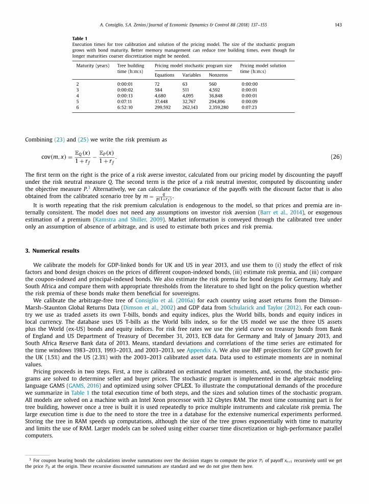
Fig. 3. Buyer and seller prices for coupon-indexed bonds increase with the base coupon rate.
Fig. 4. Buyer price sensitivity to joint changes in base coupon and target growth for coupon-indexed bonds.
large g there is downside risk that coupon payments could decrease to zero and prices are below par. For some intermediate
value, the upside potential is equal in expectations to the downside risk, and the bond prices at par.
Fig. 3 shows buyer and seller prices for different base coupon rates. The linked bonds become linearly dearer for higher
base coupon rates. In Fig. 4 we parameterize the design space and illustrate the changes of bid prices with joint changes in
base coupon and target growth. The price is equally sensitive to changes of base coupon or target growth.
The effect of bond maturity on prices is illustrated in Fig. 5 . Ceteris paribus bond prices decline with maturity, indicating
that investors expect a higher excess return for the longer maturity bonds. This price-maturity relationship is affected by
the shape of the underlying yield curve, as illustrated in the same figure by pricing the UK bond using, first, the upward
sloping yield curve of December 2013 and, then, a constant spot rate 1.47%. We also note an increase in the bid-ask spread
for longer maturities, although it remains small.
To assess the accuracy of the models in the presence of market incompleteness we look at the bid-ask spreads. In all
experiments reported above the spread is less than 3bp, indicating that for these two countries and the design parameters
of the reference bonds, the chosen assets span accurately the countries’ GDP. This may not be the case for other countries
and different choices of assets, or for different bond design parameters, or when using different time periods to calibrate

146 A. Consiglio, S.A. Zenios / Journal of Economic Dynamics & Control 88 (2018) 137–155
Fig. 5. Price vs maturity for coupon-indexed bonds. Panels (a)-(b) use the yield curve of December 2013 for discounting, the panel (c) uses a flat yield
curve at 1.47%, all other data calibrated for 2003–2013.
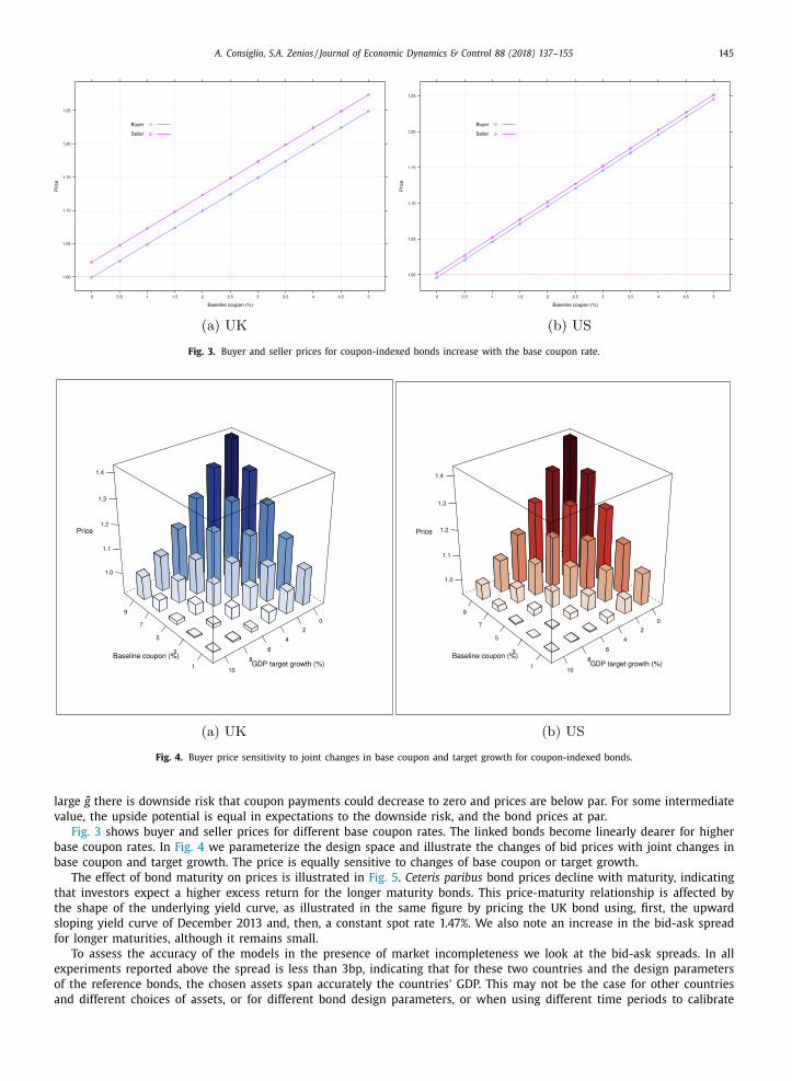
the tree. Fig. 6 illustrates the case for UK, Italy, and Portugal, with base coupon in the range 1–10% and target growth in the
range 0–10%. These spreads are small and lend credibility to the model.
Finally, we use the model to compare prices for the two bond designs, see Fig. 7 . The price of principal-indexed bonds
for different starting base coupons exhibits the same pattern as coupon-indexed bonds. Bid-ask spreads remain small, con-
sistently with the spreads for coupon-indexed bonds, and coupon-indexed bonds are cheaper than principal-indexed bonds
due to their limited downside risk.
3.2. Risk premium calibrations
Risk premia can be calculated from Eq. (26) using quantities that are available from the primal and dual pricing models. 6
We summarize first premium estimates from existing literature that provide some reference values, and then discuss our
own findings.
3.2.1. Premium estimates from the literature
Kruse et al. (2005) use their pricing model to estimate return spreads. 7 They find positive premia for Indonesia, in the
range 76bp–200bp, and negative for Venezuela, in the range 24bp–264bp. Larger premia are not always obtained for more
6 We estimate premia using both the left and right sides of Eq. (26) and obtain identical results. The premium definition in the equation is for a single-
period model, and when calculating premia for bonds of different maturities all quantities are annualized. 7 Computed as the difference of the returns (not log returns) from Tables 1 and 2 of the reference.
A. Consiglio, S.A. Zenios / Journal of Economic Dynamics & Control 88 (2018) 137–155 147
Fig. 6. Box-Whisker plots of bid-ask spreads for UK, Italy, and Portugal coupon-indexed bonds for base coupon 1–10% and target growth 0–10%. Left panel
uses US assets and right panel uses German assets to calibrate a tree.
Fig. 7. Comparing buyer prices of principal-indexed and coupon-indexed bonds. (Tree calibrated for 2003–2013. For principal-indexed bonds the coupon
rate on the x-axis is the effective coupon.)
volatile GDP returns, and the authors conclude that “comparisons between the GDP-linked bonds and the underlying gov-
ernment bond, from which the prices of the GDP-linked bonds are derived, show no clear patterns”. Bowman and Nay-
lor (2016) use CAPM and downside-CAPM to obtain a range of premia for G20 countries. Their results show that the choice
of the market portfolio has a large effect on the estimate of the risk premia across countries, and do not provide a con-
clusive answer to the policy question. The authors point out that “the cost of borrowing using GDP-linked bonds is highly
uncertain, largely due to the wide range of estimates for the growth risk premium” and they conclude that “[f]or almost half
of the countries examined, the highest estimated cost could be large enough to make the issuance of GDP-linked bonds un-
desirable”. 8 Kamstra and Shiller (2009) calibrate a CAPM model of GDP growth on the S&P 500 and estimate a premium of
150bp. Borensztein and Mauro (2004) estimate risk premia using an equilibrium model and find premia in the range 35bp–
370bp for different levels of investor risk aversion. Barr et al. (2014) use CAPM to estimate risk premium for Argentina close
to 100bp. Table 3 provides a summary of premia obtained by different authors and their underlying assumptions. Recalling
from Section 2.3 the thresholds of 250bp–350bp for volatile growth economies, and 100bp–50bp for advanced economies
with stable growth, we note that premia estimates from current literature do not unambiguously satisfy the thresholds. Our
model sheds light on this ambiguity.
8 Our model optimizes the choice of a replicating market portfolio, so it reduces the range of risk premium estimates and provides a solution to the
problem noted by these authors.

148 A. Consiglio, S.A. Zenios / Journal of Economic Dynamics & Control 88 (2018) 137–155
Table 3
Risk premium estimates by different authors.
Reference and method Bond design Market assumptions Premium estimates (bp)
and country
Borensztein–Mauro Coupon-indexed r f = 3% 100
CAPM Unspecified params. Exp. return 8%
Argentina
Kruse et al. Coupon-indexed Historical from 76–200 ∗ (Indonesia)
Options pricing and Principal-indexed Frankfurt Exchange 24–264 (Venezuela)
on underlying GDP Indonesia, Venezuela
Barr et al. Principal-indexed r f = 3 . 4% 35–370
Equilibrium model c 0 = 0 Exp. return 2.1% depending on
with risk averse investors Advanced economies risk aversion
Bowman-Naylor Unspecified params. r f = 0% > 350
CAPM G20 countries Exp. return 6.5% for half of the G20
Downside-CAPM 0–400 for UK and US
Kamstra–Shiller Principal-indexed Not provided 150
CAPM c 0 = 0
US
∗ Risk premia for Indonesia are positive. All other premia are negative and following our convention are
given in absolute value.
3.2.2. Premium estimates from the model
We now estimate risk premia for coupon-indexed bonds. Results are summarized in Fig. 8 for an emerging market and
Fig. 9 for the advanced economies. Premia are estimated for a broad range of base coupon and target growth, thus providing
additional sensitivity analysis on the design parameters. As expected, premia decrease with higher target growth rate, and
increase with base coupon. If the target growth is very high the option will never be exercised and the instrument has,
essentially, no risk premium. On the other hand, if the base coupon rate is high there is more negative impact from low
growth rates until the floor is hit, and the risk premium is higher. Looking at the slope of the curves in each panel we
observe that there is a change of roughly 25bp per 1% change in target growth. Comparing the curves for the same time-
window across panels, we observe similar change per 1% change of base coupon. Like prices, the premia appear equally
sensitive to changes of base coupon or target growth.
The results in both figures are within the ranges estimated by Barr et al. (2014) and Bowman and Naylor (2016) , but
our model provides tighter estimates. Whereas their highest premia exceed the 250bp tight threshold and, in some in-
stances, the 350bp relaxed threshold, our estimates show that there are designs below the threshold. Barr et al. (2014) argue
that for reasonable risk aversion parameters the premium is less than 350bp, and our work shows that it is below 250bp.
Bowman and Naylor (2016) conclude that, due to the wide range of premia, the cost could be large enough to make the
issuance of GDP-linked bonds undesirable, and call for “further investigation”. Our work reduces the range and reaches a
different conclusion.
A more nuanced reading is needed for advanced economies. The larger thresholds are suitable for countries that avoid
the likelihood of default from the reduced payments of GDP-linked bonds in a recession. For advanced economies default is
a neglected risk and we use a threshold of 100bp-50bp that can be acceptable to the issuing sovereign. We think of this as
an insurance premium the sovereign pays not to avoid default, a catastrophic event, but to smooth the business cycle.
From the results of the figures we make some observations pertaining to the policy question.
1. The risk premium is sensitive to the parameters of the bond design. Hence, it is hard to interpret current literature that
estimates risk premia of GDP-linked bonds without a consensus on the bond design. There is no unique premium, and
this may explain the inconclusive results from the literature cited above.
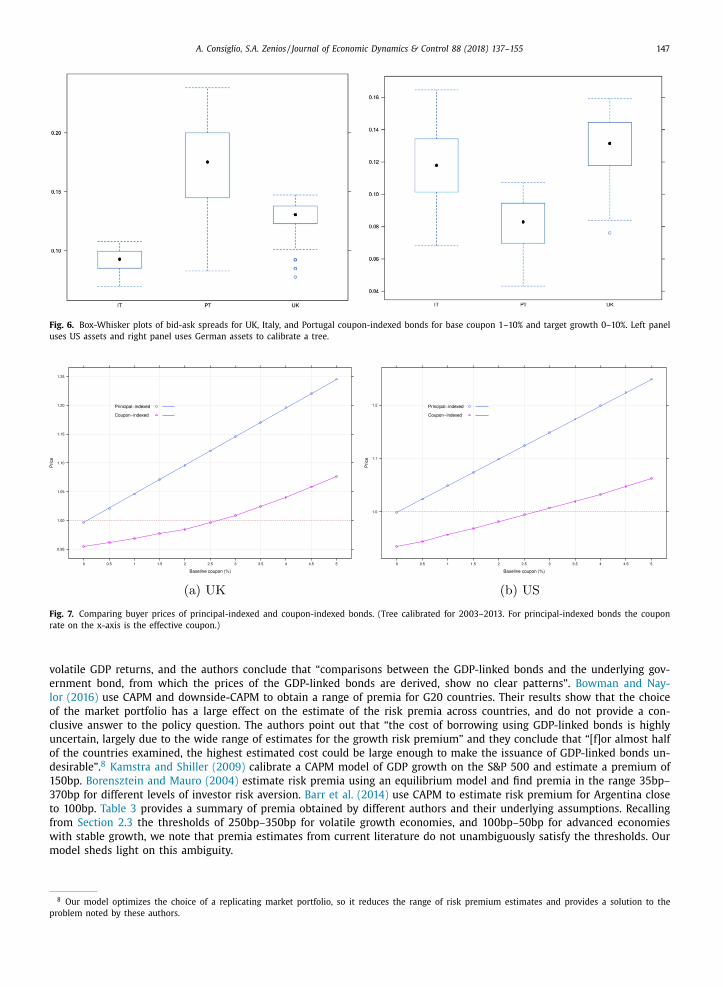
2. For Germany and the US there is a broad range of bond design parameters with risk premia attractive for sovereigns.
Designs with small premia than the 100bp threshold are acceptable. For US, a coupon-indexed bond with base coupon
1% and target growth 4% has risk premium in the range 90bp–140bp for the most recent calibrations. For Germany the
same design carries a premium less than 50bp for the most recent calibrations and slightly larger in the long run.
3. For UK a coupon-indexed bond with base coupon 1% and target growth 4% has risk premium in the 50bp–100bp range
for the more recent calibrations, and as large as 175bp for the longer time window. Increasing the base coupon to 3%
increases risk premia to 105bp for the more recent calibrations and 250bp for the longer time windows, so it is important
to determine with higher accuracy the correlations going forward. Similar conclusions hold for Italy.
4. For the emerging economy of South Africa we observe that there are several designs within the 350bp threshold, and
even within the tighter 250bp threshold when calibrated on recent data. When calibrated over the long-term horizon,
the premia for reasonable designs do not satisfy the threshold. If we believe that the correlations calibrated using the
most recent data reflect the country’s future prospects, then GDP-linked bonds are beneficial.

A. Consiglio, S.A. Zenios / Journal of Economic Dynamics & Control 88 (2018) 137–155 149
Fig. 8. Risk premia for various combinations of base coupon and target growth rates for coupon-indexed bonds for an emerging economy. Trees are
calibrated for different time windows and the three panels correspond to base coupons 1%, 3%, and 5%. Horizontal dashed lines denote the thresholds that
render GDP-linked bonds beneficial for emerging economics with volatile growth. For the most recent calibrations, that include the global financial crisis,
the premia satisfy the thresholds, and this would be a good period to issue GDP-linked bonds. However, for the correlations calibrated over the longer time
horizon we observe that the premium violates the threshold for all design parameters.
In general, there are very few designs with premia exceeding 350bp and there are several with premia less than 100bp.
Based on these thresholds our results show that GDP-linked bonds can be beneficial for sovereigns. However, risk premia,
like prices, are sensitive to input data. Our conclusions are robust when tested using different calibration windows for the
US and Germany, less so for the UK, and depend crucially on the calibrated correlations for Italy and South Africa.
3.3. Comparing coupon-indexed and principal-indexed bonds
We compare risk premia of coupon-indexed and principal-indexed bonds. We compute premia for the reference coupon-
indexed bonds and principal-indexed bonds with zero base coupon. The risk premium depends on data calibration, and
the critical parameter for principal-indexed bonds is the expected GDP growth. Hence, we use the 2003-2013 window for
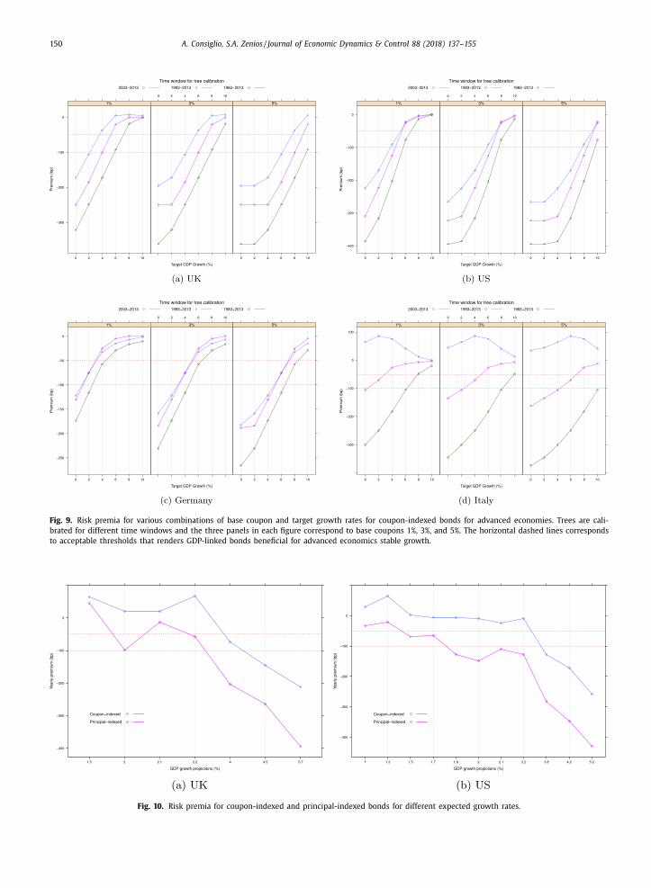
volatility and correlations, and report premia for different expected GDP growth rates in Fig. 10 .
We observe that principal-indexed bonds carry a higher premium than coupon-indexed bonds. The difference can be
as high as 200bp for high expected economic growth, but is reduced to 100bp for expected growth about 2.5%. This
observation comes with the caveat that results can change by varying the base coupon, and this brings us back to the
point that design parameters have a significant impact. A contribution of the model is to allow the analysis of alternative
designs.
Again, there are several designs of the principal-indexed bonds with premia smaller than the threshold and, hence, can
be beneficial for sovereigns. For both UK and US the premia are below the 100bp threshold for expected growth below
2.2% (UK) and 1.8% (US), and for coupon-indexed bonds for expected growth rates can go up to 4.2%(UK) and 3.5% (US).
From these results and the results in Section 3.2.2 , we conclude that GDP-linked bonds can be beneficial for sovereigns, in
both coupon-indexed and principal-indexed versions. Design choices appear more limited for the principal-indexed bonds.
Coupon-indexed bonds appear to have lower premia. However, principal-indexed bonds directly stabilize the issuer’s debt
to GDP ratio whereas coupon indexed bonds do so indirectly through lower coupon payments, so the issuer may be willing
to pay a higher risk premium on principal-indexed bonds in return for more effective debt stabilization.
150 A. Consiglio, S.A. Zenios / Journal of Economic Dynamics & Control 88 (2018) 137–155
Fig. 9. Risk premia for various combinations of base coupon and target growth rates for coupon-indexed bonds for advanced economies. Trees are cali-
brated for different time windows and the three panels in each figure correspond to base coupons 1%, 3%, and 5%. The horizontal dashed lines corresponds
to acceptable thresholds that renders GDP-linked bonds beneficial for advanced economics stable growth.
Fig. 10. Risk premia for coupon-indexed and principal-indexed bonds for different expected growth rates.
A. Consiglio, S.A. Zenios / Journal of Economic Dynamics & Control 88 (2018) 137–155 151
4. Conclusions
We have developed a model for pricing and hedging GDP-linked bonds in incomplete markets. We use stochastic pro-
gramming to sure-replicate the cashflows of the new bond with market traded assets on a discrete scenario tree. As a
byproduct of the model we obtain a hedging portfolio for investors in these novel instruments. The dual program provides
a risk neutral measure in an incomplete market, which is used to estimate risk premia. The model is applicable for different
GDP-linked bond designs, and we used it to price coupon-indexed and principal-indexed bonds. The model is calibrated for
UK and US using different calibration windows. The bid-ask spreads, prevalent in incomplete market prices, are found to
be small, thus establishing the credibility of the model. Numerical results shed light on the effect of bond design choices
—base coupon, target GDP growth rate, and maturity— on the price. We also estimate risk premia for bond designs for Ger-
many, Italy and South Africa and compare them with appropriate thresholds from the literature to shed light on the policy
question whether the risk premia of these bonds make them beneficial for sovereigns.
The model was used to estimate risk premia for two competing GDP-linked bond designs, coupon-indexed and principal-
indexed bonds. Principal-indexed bonds command a higher premium than coupon-indexed bonds. The difference can be as
high as 200bp, but is close to 100bp for expected economic growth 2.5%.
Current literature tells us that risk premia for emerging economics above 350bp render GDP-linked bonds too expensive
for sovereigns, whereas premia below a 250bp threshold benefit the sovereigns. We have shown that, for the example of
South Africa, there exists a range of bond design parameters for which a coupon-indexed bond will demand premia below
350bp, and even below 250bp when calibrated for the more recent data. For advanced economies an acceptable premium
should be smaller than 100bp–50bp, and we have shown that several designs for the UK, US, Germany and Italy have premia
within the threshold. Hence, coupon-indexed GDP-linked bonds can benefit sovereigns. Principal-indexed bonds command
a higher premium and must be carefully calibrated, and the range of acceptable design parameters is more restricted. Sen-
sitivity analysis using different calibration windows gives us confidence that these observations are robust for countries like
the US and Germany, less so for UK, and careful calibration is needed for countries with higher volatility such as Italy and
South Africa.
We emphasize that our findings, encouraging as they may be for GDP-linked bonds, deserve a nuanced reading, since
there are many inter-related risk factors and design parameters that affect prices and premia. Furthermore, some investors,
especially buy-and-hold long term entities like pension funds, will price these assets differently in the context of their
liability portfolio. Our models provide market-based benchmarks.
In conclusion, we have provided evidence in favor of GDP-linked bonds, using results for both advanced economies
and an emerging market. An interesting follow-up study would be to calibrate the model for G20 countries or emerging
economies of interest to current policy debates. Another promising avenue for further research is to apply the models to
price other derivatives linked to economic activity. In such further work emphasis should be places on the calibration of the
correlation matrices and expected growth since these are the key market parameters input to the model.
Acknowledgements
We thank Mark Joy, Angel Gavilan, Aitor Erce, Emilio Barucci, Maria Demertzis, Guntram Wolff and seminar partici-
pants at Bank of England, Bank of Canada, the Federal Reserve Bank of Philadelphia, the European Stability Mechanism and
Bruegel, for useful discussions. Rolf Strauch and an anonymous referee made several comments that led to significant im-
provements of the paper. Stavros A. Zenios holds a Marie Sklodowska-Curie fellowship funded from the European Union
Horizon 2020 research and innovation programme under grant agreement No 655092 .
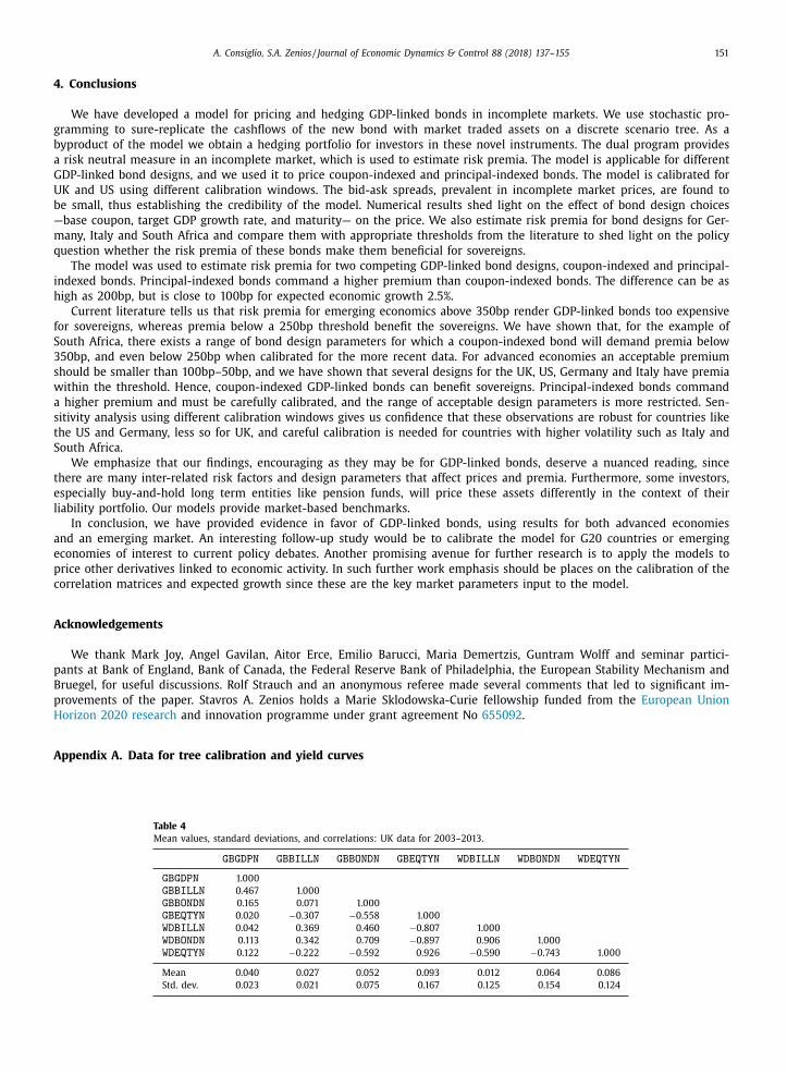
Appendix A. Data for tree calibration and yield curves
Table 4
Mean values, standard deviations, and correlations: UK data for 2003–2013.
GBGDPN GBBILLN GBBONDN GBEQTYN WDBILLN WDBONDN WDEQTYN
GBGDPN 1.0 0 0
GBBILLN 0.467 1.0 0 0
GBBONDN 0.165 0.071 1.0 0 0
GBEQTYN 0.020 −0.307 −0.558 1.0 0 0
WDBILLN 0.042 0.369 0.460 −0.807 1.0 0 0
WDBONDN 0.113 0.342 0.709 −0.897 0.906 1.0 0 0
WDEQTYN 0.122 −0.222 −0.592 0.926 −0.590 −0.743 1.0 0 0
Mean 0.040 0.027 0.052 0.093 0.012 0.064 0.086
Std. dev. 0.023 0.021 0.075 0.167 0.125 0.154 0.124

152 A. Consiglio, S.A. Zenios / Journal of Economic Dynamics & Control 88 (2018) 137–155
Table 5
Mean values, standard deviations, and correlations: UK data for 1993–2013.
GBGDPN GBBILLN GBBONDN GBEQTYN WDBILLN WDBONDN WDEQTYN
GBGDPN 1.0 0 0
GBBILLN 0.522 1.0 0 0
GBBONDN 0.200 0.314 1.0 0 0
GBEQTYN 0.025 −0.073 0.052 1.0 0 0
WDBILLN 0.050 0.367 0.316 −0.408 1.0 0 0
WDBONDN 0.112 0.302 0.672 −0.457 0.780 1.0 0 0
WDEQTYN 0.025 −0.022 0.018 0.925 −0.162 −0.311 1.0 0 0
Mean 0.045 0.041 0.077 0.082 0.024 0.074 0.071
Std. dev. 0.018 0.022 0.101 0.169 0.101 0.133 0.150
Table 6
Mean values, standard deviations, and correlations: UK data for 1983–2013.
GBGDPN GBBILLN GBBONDN GBEQTYN WDBILLN WDBONDN WDEQTYN
GBGDPN 1.0 0 0
GBBILLN 0.702 1.0 0 0
GBBONDN 0.176 0.261 1.0 0 0
GBEQTYN 0.161 0.140 0.126 1.0 0 0
WDBILLN −0.008 0.202 0.229 −0.008 1.0 0 0
WDBONDN 0.036 0.240 0.590 −0.121 0.772 1.0 0 0
WDEQTYN 0.085 0.014 0.103 0.875 0.278 0.121 1.0 0 0
Mean 0.057 0.063 0.089 0.111 0.040 0.093 0.090
Std. dev. 0.027 0.038 0.088 0.158 0.127 0.132 0.173
Table 7
Mean values, standard deviations, and correlations: US data for 2003–2013.
USGDPN USBILLN USBONDN USEQTYN WXBONDN WXEQTYN
USGDPN 1.0 0 0
USBILLN 0.448 1.0 0 0
USBONDN 0.335 0.132 1.0 0 0
USEQTYN 0.080 −0.186 −0.745 1.0 0 0
WXBONDN 0.159 −0.043 0.345 −0.037 1.0 0 0
WXEQTYN 0.179 0.043 −0.743 0.949 0.048 1.0 0 0
Mean 0.038 0.015 0.055 0.095 0.073 0.101
Std. dev. 0.023 0.017 0.118 0.197 0.060 0.248
Table 8
Mean values, standard deviations, and correlations: US data for 1993–2013.
USGDPN USBILLN USBONDN USEQTYN WXBONDN WXEQTYN
USGDPN 1.0 0 0
USBILLN 0.574 1.0 0 0
USBONDN 0.199 0.183 1.0 0 0
USEQTYN 0.166 0.052 −0.399 1.0 0 0
WXBONDN −0.029 −0.093 0.520 −0.003 1.0 0 0
WXEQTYN 0.183 −0.052 −0.555 0.847 0.074 1.0 0 0
Mean 0.045 0.028 0.073 0.090 0.081 0.073
Std. dev. 0.019 0.020 0.119 0.189 0.082 0.216
Table 9
Mean values, standard deviations, and correlations: US data for 1983–2013.
USGDPN USBILLN USBONDN USEQTYN WXBONDN WXEQTYN
USGDPN 1.0 0 0
USBILLN 0.719 1.0 0 0
USBONDN 0.205 0.254 1.0 0 0
USEQTYN 0.157 0.134 −0.193 1.0 0 0
WXBONDN −0.065 0.053 0.4 4 4 0.047 1.0 0 0
WXEQTYN 0.209 0.100 −0.253 0.767 0.290 1.0 0 0
Mean 0.052 0.041 0.087 0.107 0.097 0.096
Std. dev. 0.022 0.027 0.112 0.170 0.100 0.220

A. Consiglio, S.A. Zenios / Journal of Economic Dynamics & Control 88 (2018) 137–155 153
Table 10
Mean values, standard deviations, and correlations: German data for 2003–2013.
DEGDPN DEBILLN DEBONDN DEEQTYN WDBILLN WDBONDN WDEQTYN
DEGDPN 1.0 0 0
DEBILLN 0.082 1.0 0 0
DEBONDN 0.133 0.026 1.0 0 0
DEEQTYN −0.106 −0.349 −0.571 1.0 0 0
WDBILLN 0.116 −0.096 0.480 −0.354 1.0 0 0
WDBONDN 0.262 0.036 0.862 −0.623 0.783 1.0 0 0
WDEQTYN −0.204 −0.578 −0.379 0.909 −0.103 −0.414 1.0 0 0
Mean 0.023 0.017 0.070 0.111 −0.010 0.042 0.079
Std. dev. 0.025 0.014 0.091 0.243 0.087 0.108 0.200
Table 11
Mean values, standard deviations, and correlations: German data for 1993–2013.
DEGDPN DEBILLN DEBONDN DEEQTYN WDBILLN WDBONDN WDEQTYN
DEGDPN 1.0 0 0
DEBILLN 0.205 1.0 0 0
DEBONDN 0.075 0.127 1.0 0 0
DEEQTYN −0.089 −0.142 −0.324 1.0 0 0
WDBILLN −0.018 0.137 0.103 0.176 1.0 0 0
WDBONDN 0.084 0.255 0.698 −0.090 0.702 1.0 0 0
WDEQTYN −0.173 −0.203 −0.298 0.928 0.347 0.029 1.0 0 0
Mean 0.024 0.029 0.076 0.083 0.022 0.072 0.081
Std. dev. 0.019 0.019 0.090 0.253 0.106 0.110 0.208
Table 12
Mean values, standard deviations, and correlations: German data for 1983–2013.
DEGDPN DEBILLN DEBONDN DEEQTYN WDBILLN WDBONDN WDEQTYN
DEGDPN 1.0 0 0
DEBILLN 0.651 1.0 0 0
DEBONDN 0.067 0.079 1.0 0 0
DEEQTYN −0.034 −0.095 −0.215 1.0 0 0
WDBILLN 0.065 0.157 0.119 0.182 1.0 0 0
WDBONDN 0.168 0.223 0.678 0.022 0.714 1.0 0 0
WDEQTYN −0.067 −0.158 −0.180 0.828 0.407 0.189 1.0 0 0
Mean 0.037 0.040 0.074 0.090 0.024 0.077 0.092
Std. dev. 0.032 0.025 0.079 0.257 0.123 0.103 0.200
Table 13
Mean values, standard deviations, and correlations: Italian data for 2003–2013.
ITGDPN ITBILLN ITBONDN ITEQTYN WDBILLN WDBONDN WDEQTYN
ITGDPN 1.0 0 0
ITBILLN 0.537 1.0 0 0
ITBONDN −0.450 −0.209 1.0 0 0
ITEQTYN −0.091 −0.470 0.399 1.0 0 0
WDBILLN −0.084 −0.075 −0.038 −0.382 1.0 0 0
WDBONDN 0.162 0.144 −0.199 −0.674 0.783 1.0 0 0
WDEQTYN −0.211 −0.710 0.261 0.893 −0.106 −0.425 1.0 0 0
Mean 0.017 0.020 0.054 0.025 −0.010 0.042 0.075
Std. dev. 0.024 0.011 0.099 0.247 0.087 0.108 0.202
Table 14
Mean values, standard deviations, and correlations: Italian data for 1993–2013.
ITGDPN ITBILLN ITBONDN ITEQTYN WDBILLN WDBONDN WDEQTYN
ITGDPN 1.0 0 0
ITBILLN 0.456 1.0 0 0
ITBONDN −0.108 0.386 1.0 0 0
ITEQTYN 0.026 −0.047 0.305 1.0 0 0
WDBILLN 0.167 0.350 0.093 0.134 1.0 0 0
WDBONDN 0.185 0.484 0.316 −0.123 0.720 1.0 0 0
WDEQTYN −0.004 −0.085 0.139 0.827 0.358 0.061 1.0 0 0
Mean 0.031 0.031 0.087 0.062 0.026 0.076 0.077
Std. dev. 0.026 0.018 0.126 0.242 0.105 0.116 0.211
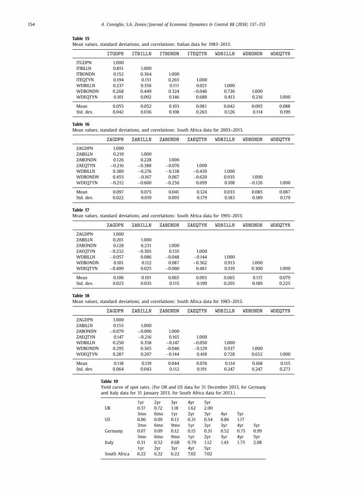
154 A. Consiglio, S.A. Zenios / Journal of Economic Dynamics & Control 88 (2018) 137–155
Table 15
Mean values, standard deviations, and correlations: Italian data for 1983–2013.
ITGDPN ITBILLN ITBONDN ITEQTYN WDBILLN WDBONDN WDEQTYN
ITGDPN 1.0 0 0
ITBILLN 0.851 1.0 0 0
ITBONDN 0.152 0.364 1.0 0 0
ITEQTYN 0.194 0.151 0.265 1.0 0 0
WDBILLN 0.237 0.356 0.111 0.021 1.0 0 0
WDBONDN 0.268 0.449 0.324 −0.046 0.736 1.0 0 0
WDEQTYN 0.101 0.092 0.146 0.680 0.413 0.216 1.0 0 0
Mean 0.055 0.052 0.103 0.081 0.042 0.095 0.088
Std. dev. 0.042 0.036 0.108 0.263 0.126 0.114 0.199
Table 16
Mean values, standard deviations, and correlations: South Africa data for 2003–2013.
ZAGDPN ZABILLN ZABONDN ZAEQTYN WDBILLN WDBONDN WDEQTYN
ZAGDPN 1.0 0 0
ZABILLN 0.219 1.0 0 0
ZABONDN 0.126 0.228 1.0 0 0
ZAEQTYN −0.216 −0.388 −0.076 1.0 0 0
WDBILLN 0.389 −0.276 −0.138 −0.439 1.0 0 0
WDBONDN 0.455 −0.167 0.067 −0.620 0.935 1.0 0 0
WDEQTYN −0.212 −0.660 −0.256 0.699 0.108 −0.126 1.0 0 0
Mean 0.097 0.075 0.041 0.124 0.033 0.085 0.087
Std. dev. 0.022 0.019 0.095 0.179 0.183 0.189 0.179
Table 17
Mean values, standard deviations, and correlations: South Africa data for 1993–2013.
ZAGDPN ZABILLN ZABONDN ZAEQTYN WDBILLN WDBONDN WDEQTYN
ZAGDPN 1.0 0 0
ZABILLN 0.201 1.0 0 0
ZABONDN 0.128 0.231 1.0 0 0
ZAEQTYN −0.232 −0.305 0.135 1.0 0 0
WDBILLN −0.057 0.086 −0.048 −0.144 1.0 0 0
WDBONDN 0.101 0.112 0.087 −0.362 0.913 1.0 0 0
WDEQTYN −0.499 0.025 −0.060 0.481 0.519 0.300 1.0 0 0
Mean 0.106 0.101 0.065 0.093 0.065 0.115 0.079
Std. dev. 0.023 0.035 0.115 0.199 0.205 0.189 0.225
Table 18
Mean values, standard deviations, and correlations: South Africa data for 1983–2013.
ZAGDPN ZABILLN ZABONDN ZAEQTYN WDBILLN WDBONDN WDEQTYN
ZAGDPN 1.0 0 0
ZABILLN 0.155 1.0 0 0
ZABONDN −0.079 −0.090 1.0 0 0
ZAEQTYN 0.147 −0.216 0.165 1.0 0 0
WDBILLN 0.250 0.358 −0.147 −0.050 1.0 0 0
WDBONDN 0.295 0.365 -0.046 −0.129 0.937 1.0 0 0
WDEQTYN 0.287 0.207 −0.144 0.418 0.728 0.652 1.0 0 0
Mean 0.118 0.119 0.044 0.076 0.114 0.168 0.115
Std. dev. 0.064 0.043 0.112 0.191 0.247 0.247 0.273
Table 19
Yield curve of spot rates. (For UK and US data for 31 December 2013, for Germany
and Italy data for 31 January 2013, for South Africa data for 2013.)
1yr 2yr 3yr 4yr 5yr
UK 0.37 0.72 1.18 1.62 2.00
3mo 6mo 1yr 2yr 3yr 4yr 5yr
US 0.06 0.09 0.13 0.31 0.54 0.86 1.17
3mo 6mo 9mo 1yr 2yr 3yr 4yr 5yr
Germany 0.07 0.09 0.12 0.15 0.31 0.52 0.75 0.99
3mo 6mo 9mo 1yr 2yr 3yr 4yr 5yr
Italy 0.31 0.52 0.68 0.79 1.12 1.43 1.75 2.08
1yr 2yr 3yr 4yr 5yr
South Africa 6.22 6.22 6.22 7.02 7.02

A. Consiglio, S.A. Zenios / Journal of Economic Dynamics & Control 88 (2018) 137–155 155
References
Baron, K. , Lange, J. , 2007. Parimutuel Applications In Finance. New Markets for New Risks. Palgrave Macmillan, UK .
Barr, D., Bush, O., Pienkowski, A., 2014. GDP −Linked Bonds and Sovereign Default. Working Paper 484. Bank of England.
Barro, R. , 2003. Optimal management of indexed and nominal debt. Ann. Econ. Finance 4, 1–15 . Benford, J. , Best, T. , Joy, M. , 2016. Sovereign GDP-linked bonds. Financial Stability Paper 39. Bank of England, London, UK .
Blanchard, O. , Mauro, P. , Acalin, J. , 2016. The case for growth-indexed bonds in advanced economies today. Policy Brief PB16–2, Peterson Institute forInternational Economics .
Borensztein, E., Chamon, M., Jeanne, O., Mauro, P., Zettelmeyer, J., 2004. Sovereign Debt Structure for Crisis Prevention. Occasional Paper 237. InternationalMonetary Fund.
Borensztein, E. , Mauro, P. , 2004. The case for GDP-indexed bonds. Econ. Pol. 165–216 .
Bowman, J., Naylor, P., 2016. GDP-linked bonds.Reserve Bank of Australia Bulletin, September Quarter. 61–68 Brooke, M. , Mendes, R. , Pienkowski, A. , Santor, E. , 2013. Sovereign default and state-contingent debt. Financial Stability Paper No. 27. Bank of England .
Caballero, R.J. , Panageas, S. , 2008. Hedging sudden stops and precautionary contractions. J. Dev. Econ.l 85 (1–2), 28–57 . Cochrane, J.H. , 2005. Asset Pricing. Princeton University Press . Revised edition.
Consiglio, A. , Carollo, A. , Zenios, S.A. , 2016a. A parsimonious model for generating arbitrage-free scenario trees. Quant. Finance 16 (2), 201–212 . Consiglio, A. , De Giovanni, D. , 2010. Pricing the option to surrender in incomplete markets. J. Risk Insurance 77 (4), 935–957 .
Consiglio, A., Tumminello, M., Zenios, S. A., 2016b. Pricing sovereign contingent convertible debt. Working Paper 16-05. The Wharton Financial Institutions
Center, University of Pennsylvania, Philadelphia. Available at https://papers.ssrn.com/sol3/papers.cfm?abstract _ id=2813427 . Consiglio, A., Zenios, S. A., 2015. The case for contingent convertible debt for sovereigns. Working Paper 15-13. The Wharton Financial Institutions Center,
University of Pennsylvania, Philadelphia. Available at http://papers.ssrn.com/sol3/papers.cfm?abstract _ id=2478380 . Costa, A., Chamon, M., Ricci, L., 2008. Is there a novelty premium on new financial instruments? The Argentine experience with GDP-indexed warrants.
Working Paper No WP/08/109. International Monetary Fund. Datz, G. , 2009. What life after default? Time horizn and the outcome of the Argentine debt restructuring deal. Rev. Int. Polit. Econ. 16 (3), 456–484 .
Dimson, E. , Marsh, P. , Staunton, M. , 2002. Triumph of the Optimists: 101 Years of Global Investment Returns. Princeton University Press, Princeton, NJ . Froot, K.A. , Scharfstein, D.S. , Stein, J. , 1989. LDC debt: Forgiveness, indexation, and investment incentives. J. Finance 44 (5), 1335–1350 .
GAMS Development Corporation 2016. GAMS –A User’s Guide. published on line, washington, DC. www.gams.com/help/topic/gams.doc/userguides/
GAMSUsersGuide.pdf . Gennaioli, N. , Shleifer, A. , Vishny, R. , 2012. Neglected risks, financial innovation, and financial fragility. J. Financ. Econ. 104 (3), 452–468 .
Griffith-Jones, S., Sharma, K., 2006. GDP-Indexed Bonds: Making it Happen. DESA Working Paper 21, United Nations. Department of Economic and SocialAffairs, New York, NY.
Guzman, M. , 2016. An analysis of Argentina’s 2001 default resolution. CIGI Papers 110, Centre for International Governance Innovation. Columbia University,New York, NY .
IMF , 2017a. State-Contingent Debt Instruments for Sovereigns.. Staff report. International Monetary Fund .
IMF , 2017b. State-Contingent Debt Instruments for Sovereigns–Annexes.. Staff report. International Monetary Fund . Kamstra, M. , Shiller, R.J. , 2009. The case for trills: Giving the people and their pension funds a stake in the wealth of the nation. Discussion Paper 1717,
Cowles Foundation for Research in Economics. Yale University, New Haven, CT . King, A.J. , 2002. Duality and martingales: A stochastic programming perspective on contingent claims. Math. Prog. Ser. B 91, 543–562 .
King, A.J. , Koivu, M. , Pennanen, T. , 2005. Calibrated option bounds. Int. J. Theor. Appl. Finance 8, 141–159 . Krugman, P. , 1988. Financing vs. forgiving a debt overhang. J. Dev. Econ. 29, 253–268 .
Kruse, S. , Meitner, M. , Schröder, M. , 2005. On the pricing of GDP linked financial products. Appl. Financ. Econ. 15 (16), 1125–1133 .
Miyajima, K., 2006. How to Evaluate GDP-Linked Warrants –Price and Repayment Capacity. In: Working Paper WP/06/85. International Monetary Fund. Obstfeld, M. , Peri, G. , 1998. Regional non-adjustment and fiscal policy. Econ. Pol. 13 (26), 205–259 .
Pliska, S.R. , 1997. Introduction to Mathematical Finance: Discrete Time Models. Blackwell, Malden, MA . Schularick, M. , Taylor, A.M. , 2012. Credit booms gone bust: Monetary policy, leverage cycles, and financial crises, 1870-2008. Am. Econ. Rev. 102 (2),
1029–1061 . Shiller, R.J. , 1993. Macro Markets: Creating Isntitutions for Managing Society’s Largest Economic Risks. Clarendon Press, New York, NY .