Journal of Computational Physics 285 (2015) 265–279

Contents lists available at ScienceDirect

Journal of Computational Physics

www.elsevier.com/locate/jcp

An asymptotic preserving unified gas kinetic scheme for grayradiative transfer equations

Wenjun Sun a, Song Jiang a, Kun Xu b,∗a Institute of Applied Physics and Computational Mathematics, P.O. Box 8009, Beijing 100088, Chinab Department of Mathematics, Hong Kong University of Science and Technology, Clear Water Bay, Kowloon, Hong Kong

a r t i c l e i n f o a b s t r a c t

Article history:Received 14 May 2014Received in revised form 5 January 2015Accepted 6 January 2015Available online 15 January 2015

Keywords:Grey radiative transfer equationsEquilibrium diffusion equationAsymptotic preservingUnified gas kinetic scheme

The solutions of radiative transport equations can cover both optical thin and optical thick regimes due to the large variation of photon’s mean-free path and its interaction with the material. In the small mean free path limit, the nonlinear time-dependent radiative transfer equations can converge to an equilibrium diffusion equation due to the intensive interaction between radiation and material. In the optical thin limit, the photon free transport mechanism will emerge. In this paper, we are going to develop an accurate and robust asymptotic preserving unified gas kinetic scheme (AP-UGKS) for the grayradiative transfer equations, where the radiation transport equation is coupled with the material thermal energy equation. The current work is based on the UGKS framework for the rarefied gas dynamics [14], and is an extension of a recent work [12] from a one-dimensional linear radiation transport equation to a nonlinear two-dimensional grayradiative system. The newly developed scheme has the asymptotic preserving (AP) property in the optically thick regime in the capturing of diffusive solution without using a cell size being smaller than the photon’s mean free path and time step being less than the photon collision time. Besides the diffusion limit, the scheme can capture the exact solution in the optical thin regime as well. The current scheme is a finite volume method. Due to the direct modeling for the time evolution solution of the interface radiative intensity, a smooth transition of the transport physics from optical thin to optical thick can be accurately recovered. Many numerical examples are included to validate the current approach.

© 2015 Elsevier Inc. All rights reserved.

1. Introduction

This paper is about the development of a numerical scheme for the solution of the time-dependent gray radiative trans-fer equations. It is well-known that the gray radiative transfer equations are modeling in the kinetic scale, where the dynamics of photon transport and collision with material is taken into account. The wide applications of this system in-clude astrophysics, inertial confinement fusion, high temperature flow systems, and many others. Due to the importance and complexity of the system, its study attracts much attention from national laboratories and academic institutes.

The gray radiative transfer equations model the radiation energy transport and the energy exchange with the background material. The properties of the background material influence greatly on the behavior of radiation transfer. For a low opac-

* Corresponding author.E-mail addresses: sun_wenjun@iapcm.ac.cn (W. Sun), jiang@iapcm.ac.cn (S. Jiang), makxu@ust.hk (K. Xu).

http://dx.doi.org/10.1016/j.jcp.2015.01.0080021-9991/© 2015 Elsevier Inc. All rights reserved.

266 W. Sun et al. / Journal of Computational Physics 285 (2015) 265–279

ity (background) material, the interaction between the radiation and material is weak, and the radiation propagates in a transparent way. The numerical method in this regime for the streaming transport equation is well defined by tracking the rays. However, for a high opacity (background) material, there is severe interaction between radiation and material with a diminishing photon mean free path. As a result, the diffusive radiative behavior will emerge. In order to solve the kinetic scale based radiative transfer equations numerically, the spatial mesh size should be comparable to the photon’s mean-free path, which is very small in the optical thick regime. Consequently, the simulation in this regime is associated with huge computational cost. To remedy these difficulties, one of the approaches is to develop the so-called asymptotic preserving (AP) scheme for the kinetic equation. When holding fixed mesh size and time step and letting the Knudsen number go to zero, the AP scheme should automatically recover the diffusion solution. The aim of this paper is to develop such an AP scheme for the gray radiation transfer equations. At the same time, the solution in the optical thin regime can be captured as well.

AP schemes were first studied in the numerical solution of steady neutron transport problems by Larsen, Morel and Miller [9], Larsen and Morel [8], and then by Jin and Levermore [4,5]. For unsteady problems, the AP schemes were constructed based on a decomposition of the distribution function between an equilibrium part and its non-equilibrium derivation, see Klar [7], and Jin, Pareschi and Toscani [6] for details. Based on the unified gas kinetic scheme (UGKS) framework [14], a rather different approach has recently been proposed by Mieussens for a linear radiation transport model [12]. The UGKS is a multi-scale direct modeling method with coupled particle transport and collision. An integral solution of the kinetic model equation has been used to construct the flow evolution around a cell interface for the flux evaluation in the finite volume scheme. This time evolution solution covers the flow physics from the kinetic scale particle free transport to the hydrodynamic scale wave propagation or diffusion limit, and the real solution used in a specific regime depends on the ratio of time step to the local particle collision time. As a result, both kinetic and hydrodynamic limiting solutions can be obtained accurately, as well as the solutions in the transition regime. Due to the un-splitting treatment for the transport and collision in UGKS, the cell size and time step used in the scheme are not limited by the particle mean free path and collision time [3,1].

In this paper, for the first time an asymptotic preserving unified gas kinetic scheme (AP-UGKS) will be developed for the gray radiation transfer equations, which are composed of radiation transport and material energy equation. The discrete-ordinate method is used to discretize the angle direction of the photon’s movement. The integral solution of the radiation intensity at a cell interface is constructed for the flux evaluation. With the angular integration on the radiation trans-port equation and the direct use of the material energy equation, for the gray radiation transfer system, two nonlinearly coupled macroscopic variables-based equations are solved at the next time level for the solutions of the radiation energy and material temperature inside each cell. For this coupled system, the resulting discrete equations give a standard five points diffusion scheme for the material temperature in a two dimensional case with Cartesian coordinates. With the up-dated radiation energy inside each cell at the next time level, the radiation intensity is explicitly obtained through the interface flux and the inner cell source term treatment. Many numerical test cases are included to validate the current approach.

This paper is organized as follows. Section 2 gives the model equations of gray radiation transfer. Section 3 reviews the construction of the unified scheme for the linear radiative equation. Section 4 presents AP-UGKS for the gray radiative transfer equations. In Section 5, many numerical tests are included to demonstrate the accuracy and robustness of the new scheme. The last section is the conclusion.

2. System of the gray radiative transfer equations

The gray radiative transfer equations describe the radiative transfer and the energy exchange between radiation and material. The equations can be written in following scaled form:⎧⎪⎪⎪⎨

⎪⎪⎪⎩ε2

c

∂ I

∂t+ ε �Ω · ∇ I = σ

(1

4πacT 4 − I

),

ε2C v∂T

∂t≡ ε2 ∂U

∂t= σ

(∫Id �Ω − acT 4

).

(2.1)

Here the spatial variable is denoted by �r , �Ω is the angular variable, and t is the time variable, I(�r, �Ω, t) is the radiation intensity, T (�r, t) is the material temperature, σ(�r, T ) is the opacity, a is the radiation constant, and c is the speed of light, ε > 0 is the Knudsen number, and U (�r, t) is the material energy density. For the simplicity of presentation, we have omitted the internal source and scattering terms in (2.1).

Eq. (2.1) is a relaxation model for the radiation intensity to the local thermodynamic equilibrium, in which the emission source is a Planckian at the local material temperature:

1

4πσacT 4.

The material temperature T (�r, t) and the material energy density U (�r, t) are related by

W. Sun et al. / Journal of Computational Physics 285 (2015) 265–279 267

∂U

∂T= C V > 0,

where CV (�r, t) is the heat capacity.As the small parameter ε → 0, Larsen et al. [10] have shown that, away from boundaries and initial times, the intensity

I approaches to a Planckian at the local temperature, i.e.,

I(0) = 1

4πac

(T (0)

)4,

and the corresponding local temperature T (0) satisfies the following nonlinear diffusion equation:

∂

∂tU

(T (0)

) + a∂

∂t

(T (0)

)4 = ∇ · ac

3σ∇(

T (0))4

. (2.2)

An asymptotic preserving (AP) scheme for the gray radiation transfer equations (2.1) is a numerical scheme that dis-cretizes (2.1) in such a way that it leads to a correct discretization of the diffusion limit (2.2) when ε is small and the scheme should be uniformly stable in ε .

With the help of the limiting equation (2.2), we shall construct our AP scheme for (2.1). First we use the discrete ordinate method to solve the radiative transfer equation (2.1). For simplicity, we consider here only the two-dimensional Cartesian spatial case. Thus in this case, the angle direction �Ω = (μ, ξ), where μ = √

1 − ζ 2 cos θ , ξ = √1 − ζ 2 sin θ with ζ ∈ [−1, 1]

is the cosine value of the angle between the propagation direction �Ω and the z-axis, while θ ∈ [0, 2π) is angle between the projection vector of �Ω onto the xy-plane and the x-axis. Due to the symmetry of angular distribution in the two dimensional Cartesian case, we need only consider ζ ≥ 0.

3. Unified scheme for the linear radiative transfer equation

The direct modeling of the interface flux in a finite volume scheme is crucial for the capturing of multi-scale radiative process in a unified scheme. In order to make our presentation clear, in this section we first construct a numerical scheme for the first equation of (2.1) only, where the term φ = acT 4 on the right hand side of this equation is supposed to be given. In the next section for the gray radiative equations, this function φ = acT 4 needs to be evaluated by solving system (4.1). Although equation (i.e. (3.1)) to be solved in this section is similar to the linear kinetic equation in [12], the numerical method is still presented in order to have a clear understanding of the scheme for the enlarged system in the next section. Even for the linear equation, the approach in [12] is extended here to two-dimensional case and to incorporate a more complete expansion of the “equilibrium state” in the integral solution of (3.1).

3.1. An AP scheme for the linear transport equation

Without loss of generality, in this subsection we consider the following linear kinetic equation in two dimension:

ε

c∂t I + μ∂x I + ξ∂y I = σ

ε

(1

2πφ − I

), (3.1)

where φ(t, x, y) is assumed to be a given function, and μ = √1 − ζ 2 cos θ , ξ = √

1 − ζ 2 sin θ with ζ ∈ [0, 1] is the cosine value of the angle between the propagation direction �Ω and the positive direction of z-axis, while θ ∈ [0, 2π) is the angle between the projection vector of �Ω onto the xy-plane and the x-axis.

As done for the usual discrete ordinate method, for Eq. (3.1) we first write the propagation direction (μ, ξ) as some discrete directions. As in [11] for example, we use the even integer N as the discrete ordinate order, then we obtain the discrete directions (μm, ξm) and their corresponding integration weights ωm for m = 1, . . . , M with M = N(N + 2)/2. For each direction (μm, ξm), we get then the direction discrete equation:

ε

c∂t Im + μm∂x Im + ξm∂y Im = σ

ε

(1

2πφ − Im

). (3.2)

Let xi = i�x, y j = j�y and tn = n�t (i, j, n ∈ Z) be the uniform mesh in Cartesian coordinates, where these �x, �yand �t are the mesh sizes in the x-, y- and t-direction respectively; and let (i, j) denote the cell {(x, y); xi−1/2 < x <xi+1/2, y j−1/2 < y < y j+1/2}, where xi−1/2 = (i − 1

2 )�x and y j−1/2 = ( j − 12 )�y are the cell interfaces.

Ini, j,m is the cell averaged value of variable Im at time tn in cell (i, j) with cell center (xi, j, yi, j). Then, we integrate

Eq. (3.2) over the cell (i, j) and from time tn to tn + �t , a conservative finite volume numerical scheme for Eq. (3.2) is of the form

In+1i, j,m = In

i, j,m + �t

�x(Fi−1/2, j,m − Fi+1/2, j,m) + �t

�y(Hi, j−1/2,m − Hi, j+1/2,m)

+ c�t

{σ

2

(1

φ − I i, j,m

)}, (3.3)

ε 2π i, j

268 W. Sun et al. / Journal of Computational Physics 285 (2015) 265–279

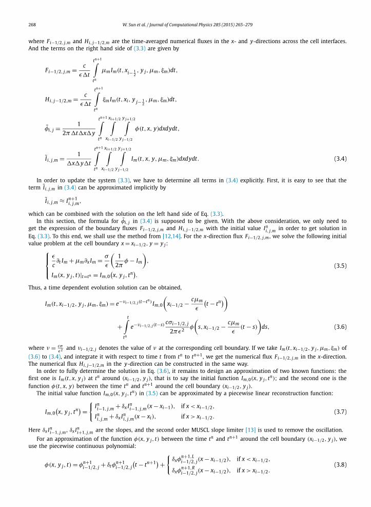
where Fi−1/2, j,m and Hi, j−1/2,m are the time-averaged numerical fluxes in the x- and y-directions across the cell interfaces. And the terms on the right hand side of (3.3) are given by

Fi−1/2, j,m = c

ε�t

tn+1∫tn

μm Im(t, xi− 12, y j,μm, ξm)dt,

Hi, j−1/2,m = c

ε�t

tn+1∫tn

ξm Im(t, xi, y j− 12,μm, ξm)dt,

φi, j = 1

2π�t�x�y

tn+1∫tn

xi+1/2∫xi−1/2

y j+1/2∫y j−1/2

φ(t, x, y)dxdydt,

I i, j,m = 1

�x�y�t

tn+1∫tn

xi+1/2∫xi−1/2

y j+1/2∫y j−1/2

Im(t, x, y,μm, ξm)dxdydt. (3.4)

In order to update the system (3.3), we have to determine all terms in (3.4) explicitly. First, it is easy to see that the term I i, j,m in (3.4) can be approximated implicitly by

I i, j,m ≈ In+1i, j,m,

which can be combined with the solution on the left hand side of Eq. (3.3).In this section, the formula for φi, j in (3.4) is supposed to be given. With the above consideration, we only need to

get the expression of the boundary fluxes Fi−1/2, j,m and Hi, j−1/2,m with the initial value Ini, j,m in order to get solution in

Eq. (3.3). To this end, we shall use the method from [12,14]. For the x-direction flux Fi−1/2, j,m , we solve the following initial value problem at the cell boundary x = xi−1/2, y = y j :⎧⎪⎨

⎪⎩ε

c∂t Im + μm∂x Im = σ

ε

(1

2πφ − Im

),

Im(x, y j, t)|t=tn = Im,0(x, y j, tn

).

(3.5)

Thus, a time dependent evolution solution can be obtained,

Im(t, xi−1/2, y j,μm, ξm) = e−νi−1/2, j(t−tn) Im,0

(xi−1/2 − cμm

ε

(t − tn))

+t∫

tn

e−νi−1/2, j(t−s) cσi−1/2, j

2πε2φ

(s, xi−1/2 − cμm

ε(t − s)

)ds, (3.6)

where ν = cσε2 and νi−1/2, j denotes the value of ν at the corresponding cell boundary. If we take Im(t, xi−1/2, y j, μm, ξm) of

(3.6) to (3.4), and integrate it with respect to time t from tn to tn+1, we get the numerical flux Fi−1/2, j,m in the x-direction. The numerical flux Hi, j−1/2,m in the y-direction can be constructed in the same way.

In order to fully determine the solution in Eq. (3.6), it remains to design an approximation of two known functions: the first one is Im(t, x, y j) at tn around (xi−1/2, y j), that is to say the initial function Im,0(x, y j, tn); and the second one is the function φ(t, x, y) between the time tn and tn+1 around the cell boundary (xi−1/2, y j).

The initial value function Im,0(x, y j, tn) in (3.5) can be approximated by a piecewise linear reconstruction function:

Im,0(x, y j, tn) =

{Ini−1, j,m + δx In

i−1, j,m(x − xi−1), if x < xi−1/2,

Ini, j,m + δx In

i, j,m(x − xi), if x > xi−1/2.(3.7)

Here δx Ini−1, j,m , δx In

i+1, j,m are the slopes, and the second order MUSCL slope limiter [13] is used to remove the oscillation.

For an approximation of the function φ(x, y j, t) between the time tn and tn+1 around the cell boundary (xi−1/2, y j), we use the piecewise continuous polynomial:

φ(x, y j, t) = φn+1i−1/2, j + δtφ

n+1i−1/2, j

(t − tn+1) +

{δxφ

n+1,Li−1/2, j(x − xi−1/2), if x < xi−1/2,

δxφn+1,R

(x − xi−1/2), if x > xi−1/2.(3.8)

i−1/2, j

W. Sun et al. / Journal of Computational Physics 285 (2015) 265–279 269

Here φn+1i−1/2, j is the cell boundary value which is supposed to be known in Eq. (3.1), and the left and right one-sided finite

differences are given by

δxφn+1,Li−1/2, j = φn+1

i−1/2, j − φn+1i−1, j

�x/2, δxφ

n+1,Ri−1/2, j = φn+1

i, j − φn+1i−1/2, j

�x/2.

For the time derivative δtφn+1i−1/2, j , we use

δtφn+1i−1/2, j = φn+1

i−1/2, j − φni−1/2, j

�t.

The boundary flux in the y-direction can be constructed in the same way. This completes the construction of the nu-merical scheme for Eq. (3.1).

In the following subsection, we give the asymptotic analysis of the above constructed numerical scheme and show that the scheme is asymptotically preserving.

3.2. Asymptotic analysis of the numerical scheme for the linear transport equation

In this subsection, we adapt the idea from [12] to show that the scheme constructed in the above subsection is asymp-totic preserving. We start with a detailed formulation for the numerical flux. Given the above constructions, the numerical flux

Fi−1/2, j,m = cμm

ε�t

tn+1∫tn

Im(t, xi−1/2, y j,μm, ξm)dt

can be exactly computed by using the expressions (3.6), (3.7) and (3.8), which is

Fi−1/2, j,m = Ai−1/2, jμm(

I−i−1/2, j,m1μm>0 + I+i−1/2, j,m1μm<0) + Ci−1/2, jμmφn+1

i−1/2, j

+ Di−1/2, j(μ2

mδxφn+1,Li−1/2, j1μm>0 + μ2

mδxφn+1,Ri−1/2, j1μm<0

)+ Bi−1/2, j

(μ2

mδx Ini−1, j,m1μm>0 + μ2

mδx Ini, j,m1μm<0

)+ Ei−1/2, jμmδtφ

n+1i−1/2, j. (3.9)

where we use I−i−1/2, j,m , I+i−1/2, j,m to denote the boundary values, which are

I−i−1/2, j,m = Ii−1, j,m + �x

2δx In

i−1, j,m,

I+i−1/2, j,m = Ii, j,m − �x

2δx In

i, j,m,

and the coefficients in (3.9) are given by

A = c

ε�tν

(1 − e−ν�t),

C = c2σ

2π�tε3ν

(�t − 1

ν

(1 − e−ν�t)),

D = − c3σi−1, j

2π�tε4ν2

(�t

(1 + e−ν�t) − 2

ν

(1 − e−ν�t)),

B = − c2

ε2ν2�t

(1 − e−ν�t − ν�te−ν�t),

E = c2σ

2πε3ν3�t

(1 − e−ν�t − ν�te−ν�t − 1

2(ν�t)2

), (3.10)

and we recall that ν = cσε2 . With the expression (3.10), we have

Ai−1/2, j = A(�t, ε,σi−1/2, j, νi−1/2, j),

Ci−1/2, j = C(�t, ε,σi−1/2, j, νi−1/2, j),

Di−1/2, j = D(�t, ε,σi−1/2, j, νi−1/2, j),

Bi−1/2, j = B(�t, ε,σi−1/2, j, νi−1/2, j),

Ei−1/2, j = H(�t, ε,σi−1/2, j, νi−1/2, j). (3.11)

270 W. Sun et al. / Journal of Computational Physics 285 (2015) 265–279

We should point out here that even with the interface solution (3.6), in order to obtain a consistent diffusion limit flux, we have to correctly define the coefficients, such as σ , at a cell boundary using the values from the two neighboring cells in the above flux expression (3.9).

The behavior of the scheme in the small ε limit is completely determined by the property of the coefficient functions that are given by

Proposition 1. Let σ be positive. Then as ε tends to zero, we have

• A(�t, ε, σ , ν) tends to 0;• B(�t, ε, σ , ν) tends to 0;• D(�t, ε, σ , ν) tends to −c/(2πσ).

Thus, the corresponding macroscopic diffusion flux (Diff)n+1i−1/2, j , defined by

(Diff)n+1i−1/2, j =

⟨cμ

ε�t

tn+1∫tn

I(t, xi−1/2, y j,μ, ξ)dt

⟩

=∫

cμ

2πε�t

tn+1∫tn

I(t, xi−1/2, y j,μ, ξ)dtdμdξ, (3.12)

has the following limit:

(Diff)n+1i−1/2, j = 1

2π

M∑m=1

ωmμm Im(t, xi−1/2, y j,μm, ξm)−→ε→0

−(

c

6σi−1/2, jδxφ

n+1,Li−1/2, j + c

6σi−1/2, jδxφ

n+1,Ri−1/2, j

)

= − c

3σi−1/2, j

φn+1i, j − φn+1

i−1, j

�x. (3.13)

The limit (3.13) gives a numerical flux of the asymptotic limiting equation which is the standard three points scheme for the diffusion equation in the one-dimensional case, and it will become the five points scheme in the two-dimensional case.

4. AP-UGKS for gray radiative transfer equations

In this section, based on the UGKS for the linear transfer equation (3.1) in the above section, we will present the AP-UGKS for the gray radiation transfer equations (2.1). In this case, we have to give the detailed expression φ in (3.3) and the cell boundary formula φ(xi−1/2, y j, t) in (3.8).

As in the above section, we denote φ = acT 4, and ρ = ∫Id �Ω . Then we take the angle integration of the first equation in

(2.1) and obtain the following macroscopic system:⎧⎪⎪⎨⎪⎪⎩

ε2

c

∂ρ

∂t+ ε∇ · 〈 �Ω I〉 = σ(φ − ρ),

ε2C v∂T

∂t≡ ε2 ∂U

∂t= σ(ρ − φ),

(4.1)

where we have denoted the angle vector integration 〈 �Ω I〉 by

〈 �Ω I〉 =∫

�Ω Id �Ω.

In order to obtain the macro-quantities ρ and φ at the next time step through Eq. (4.1), we first define an exact rela-tionship between the material energy density U and the radiation energy density φ = acT 4 by

β(x, t) = ∂φ

∂U= dφ

dT

dT

dU= 4acT 3

C v(T ). (4.2)

Then the system (4.1) can be rewritten as⎧⎪⎪⎨⎪⎪⎩

ε2

c

∂ρ

∂t+ ε∇ · 〈 �Ω I〉 = σ(φ − ρ),

ε2 ∂φ = βσ(ρ − φ).

(4.3)

∂t

W. Sun et al. / Journal of Computational Physics 285 (2015) 265–279 271

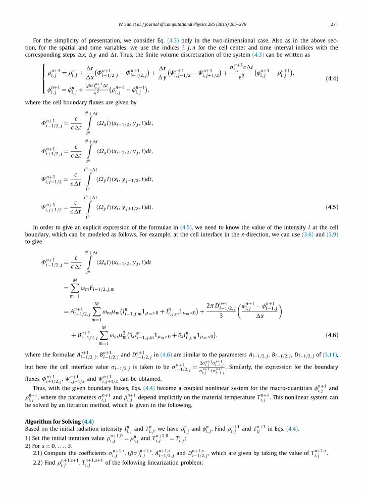
For the simplicity of presentation, we consider Eq. (4.3) only in the two-dimensional case. Also as in the above sec-tion, for the spatial and time variables, we use the indices i, j, n for the cell center and time interval indices with the corresponding steps �x, �y and �t . Thus, the finite volume discretization of the system (4.3) can be written as⎧⎪⎪⎨

⎪⎪⎩ρn+1

i, j = ρni, j + �t

�x

(Φn+1

i−1/2, j − Φn+1i+1/2, j

) + �t

�y

(Ψ n+1

i, j−1/2 − Ψ n+1i, j+1/2

) + σ n+1i, j c�t

ε2

(φn+1

i, j − ρn+1i, j

),

φn+1i, j = φn

i, j + (βσ )n+1i, j �t

ε2

(ρn+1

i, j − φn+1i, j

),

(4.4)

where the cell boundary fluxes are given by

Φn+1i−1/2, j = c

ε�t

tn+�t∫tn

〈Ωx I〉(xi−1/2, y j, t)dt,

Φn+1i+1/2, j = c

ε�t

tn+�t∫tn

〈Ωx I〉(xi+1/2, y j, t)dt,

Ψ n+1i, j−1/2 = c

ε�t

tn+�t∫tn

〈Ωy I〉(xi, y j−1/2, t)dt,

Ψ n+1i, j+1/2 = c

ε�t

tn+�t∫tn

〈Ωy I〉(xi, y j+1/2, t)dt. (4.5)

In order to give an explicit expression of the formulae in (4.5), we need to know the value of the intensity I at the cell boundary, which can be modeled as follows. For example, at the cell interface in the x-direction, we can use (3.6) and (3.9)to give

Φn+1i−1/2, j = c

ε�t

tn+�t∫tn

〈Ωx I〉(xi−1/2, y j, t)dt

=M∑

m=1

ωm Fi−1/2, j,m

= An+1i−1/2, j

M∑m=1

ωmμm(

Ini−1, j,m1μm>0 + In

i, j,m1μm<0) + 2π Dn+1

i−1/2, j

3

(φn+1

i, j − φn+1i−1, j

�x

)

+ Bn+1i−1/2, j

M∑m=1

ωmμ2m

(δx In

i−1, j,m1μm>0 + δx Ini, j,m1μm<0

). (4.6)

where the formulae An+1i−1/2, j , Bn+1

i−1/2, j and Dn+1i−1/2, j in (4.6) are similar to the parameters Ai−1/2, j , Bi−1/2, j , Di−1/2, j of (3.11),

but here the cell interface value σi−1/2, j is taken to be σ n+1i−1/2, j = 2σn+1

i, j σn+1i−1, j

σn+1i, j +σn+1

i−1, j

. Similarly, the expression for the boundary

fluxes Φn+1i+1/2, j , Ψ

n+1i, j−1/2 and Ψ n+1

i, j+1/2 can be obtained.

Thus, with the given boundary fluxes, Eqs. (4.4) become a coupled nonlinear system for the macro-quantities φn+1i, j and

ρn+1i, j , where the parameters σ n+1

i, j and βn+1i, j depend implicitly on the material temperature T n+1

i, j . This nonlinear system can be solved by an iteration method, which is given in the following.

Algorithm for Solving (4.4)Based on the initial radiation intensity In

i, j and T ni, j , we have ρn

i, j and φni, j . Find ρn+1

i, j and T n+1i j in Eqs. (4.4).

1) Set the initial iteration value ρn+1,0i, j = ρn

i, j and T n+1,0i, j = T n

i, j ;2) For s = 0, . . . , S .

2.1) Compute the coefficients σ n+1,si, j , (βσ )

n+1,si, j , An+1,s

i−1/2, j and Dn+1,si−1/2, j , which are given by taking the value of T n+1,s

i, j .

2.2) Find ρn+1,s+1, T n+1,s+1 of the following linearization problem:

i, j i, j

272 W. Sun et al. / Journal of Computational Physics 285 (2015) 265–279

⎧⎪⎪⎪⎪⎪⎨⎪⎪⎪⎪⎪⎩

ρn+1,s+1i, j = ρn

i, j + �t

�x

(Φ

n+1,si−1/2, j − Φ

n+1,si+1/2, j

) + �t

�y

(Ψ

n+1,si, j−1/2 − Ψ

n+1,si, j+1/2

)+ σn+1,s

i, j c�t

ε2

(φ

n+1,s+1i, j − ρn+1,s+1

i, j

),

φn+1,s+1i, j = φn

i, j + (βσ )n+1,si, j �t

ε2

(ρn+1,s+1

i, j − φn+1,s+1i, j

),

(4.7)

here the interface numerical flux Φn+1,si−1/2, j has the similar form as (4.6), which can be written as

Φn+1,si−1/2, j = An+1,s

i−1/2, j

M∑m=1

ωmμm(

Ini−1, j,m1μm>0 + In

i, j,m1μm<0) + 2π Dn+1,s

i−1/2, j

3

(φ

n+1,s+1i, j − φ

n+1,s+1i−1, j

�x

)

+ Bn+1,si−1/2, j

M∑m=1

ωmμ2m

(δx In

i−1, j,m1μm>0 + δx Ini, j,m1μm<0

).

2.3) For the linear system (4.7), use the Gauss–Sidel iteration to solve the resulting linear algebraic system.2.4) Compute the relative iteration error, if converges, then stop the iteration.

3) Set the final value ρn+1i, j = ρn+1,s+1

i, j and T n+1i, j = T n+1,s+1

i, j .End

After obtaining φn+1i, j by the above iteration method, we take φ in (3.4) to be

φ = 1

2πφn+1

i, j , (4.8)

and the cell boundary value φn+1i−1/2, j in (3.8) to be

φn+1i−1/2, j = 1

2

(φn+1

i−1, j + φn+1i, j

). (4.9)

The parameter σi−1/2, j in (3.11) is determined by σ n+1i−1/2, j = 2σn+1

i, j σn+1i−1, j

σn+1i, j +σn+1

i−1, j

with the above updated material temperature T n+1i, j .

Thus, the interface flux for the first equation of the system (2.1) is fully obtained, such as by the formula (3.9) for Fi−1/2, j . The remaining fluxes Fi+1/2, j , Hi, j−1/2 and Hi, j+1/2 can be obtained similarly. Then the first equation in (2.1) can be solved by the following scheme

In+1i, j,m = In

i, j,m + �t

�x(Fi−1/2, j − Fi+1/2, j) + �t

�y(Hi, j−1/2 − Hi, j+1/2) + c�tσ n+1

i, j

ε2

(1

2πφn+1

i, j − In+1i, j,m

). (4.10)

The final step is to solve the second equation in (2.1) to obtain the final material temperature with the newly obtained value In+1

i, j,m , the solution of which is directly given by

φn+1i, j = φn

i, j + �t(βσ )n+1i, j

∑Mm=1 ωm In+1

i, j,m/ε2

1 + �t(βσ )n+1i, j /ε2

. (4.11)

Based on (4.11), we immediately obtain the material temperature T n+1i, j = (φn+1

i, j /(ac))1/4. This completes the construction of the AP-UGKS for the gray radiation transfer equations (2.1). We summarize the steps of our AP-UGKS in the following.

Loop of the AP-UGKS: Given Ini, j,m and T n

i, j , we have ρni, j and φn

i, j . Find In+1 and T n+1.

1) Solve the system (4.4) to obtain φn+1i, j , ρn+1

i, j ;

2) Using the obtained value φn+1i, j from the above step, to solve the resulting equation (4.10) to get In+1

i, j,m;

3) Using the solution In+1i, j,m , to solve the resulting equation by using the explicit expression (4.11) to get the new value φn+1

i, j . Then, to give the final material temperature T n+1

i, j = (φn+1i, j /(ac))1/4.

4) Goto 1) for the next computational step.

Next, we analyze the AP property of the above scheme through the following proposition.

Proposition 2. Let σ be positive. Then as ε tends to zero, the numerical scheme given by (4.4), (4.10) and (4.11) approaches to the standard implicit diffusion scheme for the diffusion limit equation (2.2).

W. Sun et al. / Journal of Computational Physics 285 (2015) 265–279 273

Proof. In view of the order ε−2 term in Eq. (4.10), as the parameter ε tends to zero, we have

In+1i, j,m → 1

2πφn+1

i, j .

To integrate the above equation with the angle variable, as ε → 0, we get

ρn+1i, j → φn+1

i, j = ac(T n+1

i, j

)4. (4.12)

Then, for the order ε−1 terms in Eq. (4.10), such as the flux F n+1i−1/2, j from the formula (3.9), with the integration of the

flux F n+1i−1/2, j over the angle variable, we can obtain the macro flux Φn+1

i−1/2, j from Eq. (4.6). By Proposition 1, as ε → 0, we get

Φn+1i−1/2, j → − c

3σ n+1i−1/2, j

Φn+1i, j − Φn+1

i−1, j

�x. (4.13)

Similarly, in the diffusive limit ε → 0, the other macro interface fluxes go to

Φn+1i+1/2, j → − c

3σ n+1i+1/2, j

Φn+1i, j − Φn+1

i+1, j

�x,

Ψ n+1i, j−1/2 → − c

3σ n+1i, j−1/2

Φn+1i, j − Φn+1

i, j−1

�y,

Ψ n+1i, j+1/2 → − c

3σ n+1i, j+1/2

Φn+1i, j − Φn+1

i, j+1

�y. (4.14)

Therefore, with Eqs. (4.10), (4.11), and the integration over the angle variable, we can have

ρn+1i, j = ρn

i, j + �t

�x

(− c

3σ n+1i−1/2, j

Φn+1i, j − Φn+1

i−1, j

�x+ c

3σ n+1i+1/2, j

Φn+1i, j − Φn+1

i+1, j

�x

)

+ �t

�y

(− c

3σ n+1i, j−1/2

Φn+1i, j − Φn+1

i, j−1

�y+ c

3σ n+1i, j+1/2

Φn+1i, j − Φn+1

i, j+1

�y

)− c

(φn+1

i, j − φni, j

)/βn+1

i, j . (4.15)

With the connection (4.12), Eq. (4.15) is the standard five points scheme for the limiting diffusion equation (2.2). So, the current scheme for the gray radiative transfer equations (2.1) is an asymptotic preserving method. �

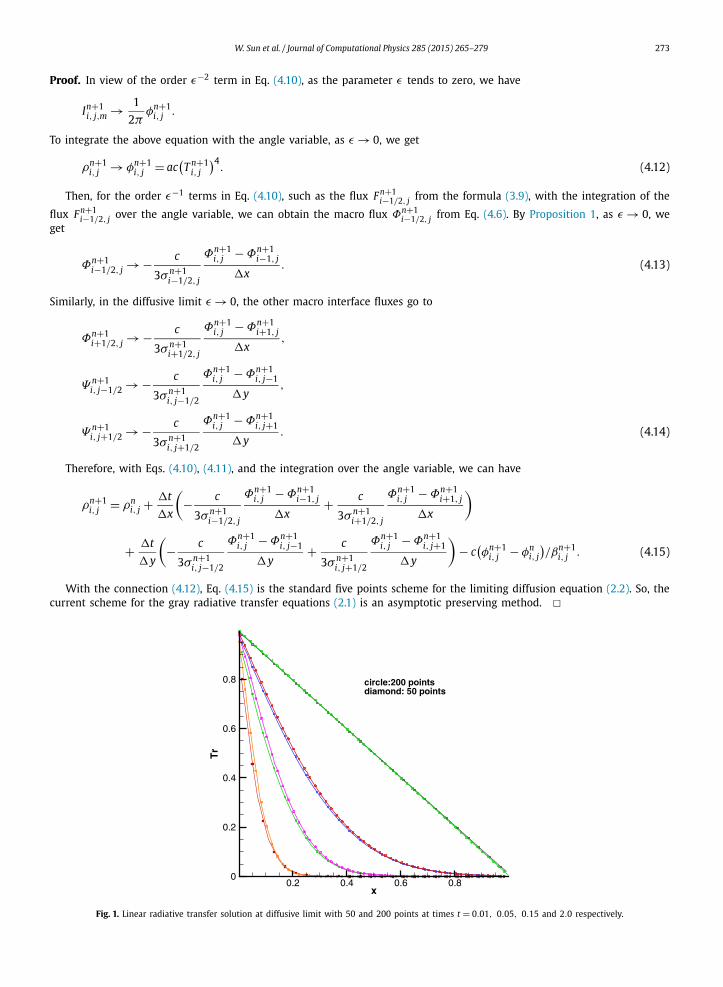
Fig. 1. Linear radiative transfer solution at diffusive limit with 50 and 200 points at times t = 0.01, 0.05, 0.15 and 2.0 respectively.

274 W. Sun et al. / Journal of Computational Physics 285 (2015) 265–279

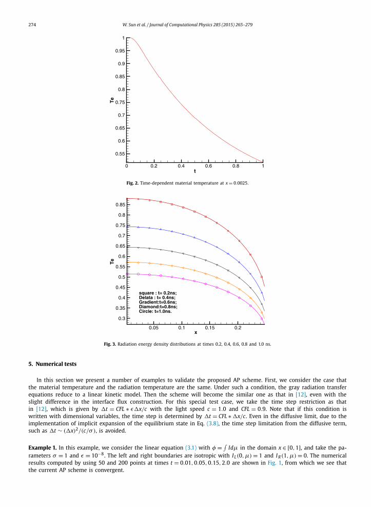
Fig. 2. Time-dependent material temperature at x = 0.0025.

Fig. 3. Radiation energy density distributions at times 0.2, 0.4, 0.6, 0.8 and 1.0 ns.

5. Numerical tests

In this section we present a number of examples to validate the proposed AP scheme. First, we consider the case that the material temperature and the radiation temperature are the same. Under such a condition, the gray radiation transfer equations reduce to a linear kinetic model. Then the scheme will become the similar one as that in [12], even with the slight difference in the interface flux construction. For this special test case, we take the time step restriction as that in [12], which is given by �t = CFL ∗ ε�x/c with the light speed c = 1.0 and CFL = 0.9. Note that if this condition is written with dimensional variables, the time step is determined by �t = CFL ∗ �x/c. Even in the diffusive limit, due to the implementation of implicit expansion of the equilibrium state in Eq. (3.8), the time step limitation from the diffusive term, such as �t ∼ (�x)2/(c/σ ), is avoided.

Example 1. In this example, we consider the linear equation (3.1) with φ = ∫Idμ in the domain x ∈ [0, 1], and take the pa-

rameters σ = 1 and ε = 10−8. The left and right boundaries are isotropic with I L(0, μ) = 1 and I R(1, μ) = 0. The numerical results computed by using 50 and 200 points at times t = 0.01, 0.05, 0.15, 2.0 are shown in Fig. 1, from which we see that the current AP scheme is convergent.

W. Sun et al. / Journal of Computational Physics 285 (2015) 265–279 275

Fig. 4. The radiation front profiles at times 15, 30, 45, 60 and 74 ns respectively of Example 3.

Fig. 5. The material temperature from UGKS simulation and from the diffusion equation solution at time 74 ns of Example 3.

In the following examples, we simulate different gray radiative transfer problems. In the computations, the unit of the length is taken to be centimeter, the mass unit is gramme (g), the time unit is nanosecond (ns), the temperature unit is kilo electron-volt (keV), and the energy unit is 109 Joules (GJ). And under the above units, the light speed is 29.98 cm/ns and the radiation constant a is 0.01372 GJ/cm3-keV4. The Courant number CFL is taken to be 0.8 in the following numerical testing.

Example 2. In this example we use a temperature-independent opacity of σ = 100 cm−1 and a temperature-independent heat capacity of CV = 0.01 GJ/cm3-keV4. Consider a one-dimensional slab of length 0.25 cm which is initially at equilibrium at 1 keV. For this problem we impose the reflection condition on the left boundary and an incident Planckian source condition at 0.1 keV on the right boundary. We take the spatial step �x = 0.005 and the final simulation time is 1 ns. For this test case, we take the fixed time step �t = 0.005d0. Fig. 2 presents material temperature vs. time at x = 0.0025, and Fig. 3 is the computed spatial distributions of the radiation energy density at five different output times of 0.2, 0.4, 0.6, 0.8 and 1.0 ns respectively. Accurate solutions have been obtained.

Example 3 (Marshak wave-2B). In this example we take the absorption/emission coefficient to be σ = 100/T 3 cm2/g, the specific heat to be 0.1 GJ/g/keV, and the density to be 3.0 g/cm3. The initial material temperature T is set to be 10−6 keV.

276 W. Sun et al. / Journal of Computational Physics 285 (2015) 265–279

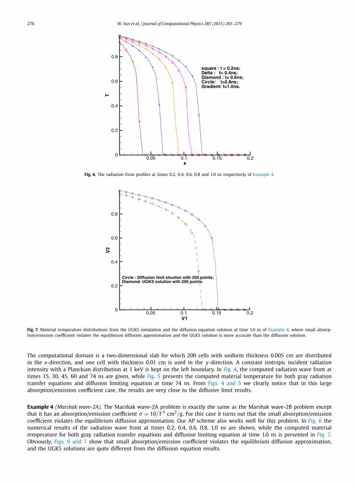
Fig. 6. The radiation front profiles at times 0.2, 0.4, 0.6, 0.8 and 1.0 ns respectively of Example 4.

Fig. 7. Material temperature distributions from the UGKS simulation and the diffusion equation solution at time 1.0 ns of Example 4, where small absorp-tion/emission coefficient violates the equilibrium diffusion approximation and the UGKS solution is more accurate than the diffusion solution.

The computational domain is a two-dimensional slab for which 200 cells with uniform thickness 0.005 cm are distributed in the x-direction, and one cell with thickness 0.01 cm is used in the y-direction. A constant isotropic incident radiation intensity with a Planckian distribution at 1 keV is kept on the left boundary. In Fig. 4, the computed radiation wave front at times 15, 30, 45, 60 and 74 ns are given, while Fig. 5 presents the computed material temperature for both gray radiation transfer equations and diffusion limiting equation at time 74 ns. From Figs. 4 and 5 we clearly notice that in this large absorption/emission coefficient case, the results are very close to the diffusive limit results.

Example 4 (Marshak wave-2A). The Marshak wave-2A problem is exactly the same as the Marshak wave-2B problem except that it has an absorption/emission coefficient σ = 10/T 3 cm2/g. For this case it turns out that the small absorption/emission coefficient violates the equilibrium diffusion approximation. Our AP scheme also works well for this problem. In Fig. 6 the numerical results of the radiation wave front at times 0.2, 0.4, 0.6, 0.8, 1.0 ns are shown, while the computed material temperature for both gray radiation transfer equations and diffusion limiting equation at time 1.0 ns is presented in Fig. 7. Obviously, Figs. 6 and 7 show that small absorption/emission coefficient violates the equilibrium diffusion approximation, and the UGKS solutions are quite different from the diffusion equation results.

W. Sun et al. / Journal of Computational Physics 285 (2015) 265–279 277

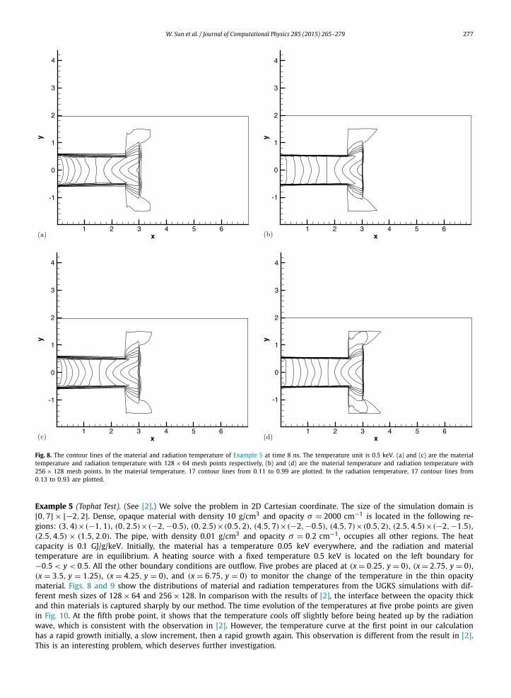
Fig. 8. The contour lines of the material and radiation temperature of Example 5 at time 8 ns. The temperature unit is 0.5 keV. (a) and (c) are the material temperature and radiation temperature with 128 × 64 mesh points respectively, (b) and (d) are the material temperature and radiation temperature with 256 × 128 mesh points. In the material temperature, 17 contour lines from 0.11 to 0.99 are plotted. In the radiation temperature, 17 contour lines from 0.13 to 0.93 are plotted.

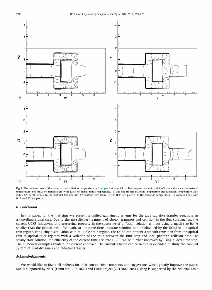
Example 5 (Tophat Test). (See [2].) We solve the problem in 2D Cartesian coordinate. The size of the simulation domain is [0, 7] × [−2, 2]. Dense, opaque material with density 10 g/cm3 and opacity σ = 2000 cm−1 is located in the following re-gions: (3, 4) ×(−1, 1), (0, 2.5) ×(−2, −0.5), (0, 2.5) ×(0.5, 2), (4.5, 7) ×(−2, −0.5), (4.5, 7) ×(0.5, 2), (2.5, 4.5) ×(−2, −1.5), (2.5, 4.5) × (1.5, 2.0). The pipe, with density 0.01 g/cm3 and opacity σ = 0.2 cm−1, occupies all other regions. The heat capacity is 0.1 GJ/g/keV. Initially, the material has a temperature 0.05 keV everywhere, and the radiation and material temperature are in equilibrium. A heating source with a fixed temperature 0.5 keV is located on the left boundary for −0.5 < y < 0.5. All the other boundary conditions are outflow. Five probes are placed at (x = 0.25, y = 0), (x = 2.75, y = 0), (x = 3.5, y = 1.25), (x = 4.25, y = 0), and (x = 6.75, y = 0) to monitor the change of the temperature in the thin opacity material. Figs. 8 and 9 show the distributions of material and radiation temperatures from the UGKS simulations with dif-ferent mesh sizes of 128 × 64 and 256 × 128. In comparison with the results of [2], the interface between the opacity thick and thin materials is captured sharply by our method. The time evolution of the temperatures at five probe points are given in Fig. 10. At the fifth probe point, it shows that the temperature cools off slightly before being heated up by the radiation wave, which is consistent with the observation in [2]. However, the temperature curve at the first point in our calculation has a rapid growth initially, a slow increment, then a rapid growth again. This observation is different from the result in [2]. This is an interesting problem, which deserves further investigation.

278 W. Sun et al. / Journal of Computational Physics 285 (2015) 265–279

Fig. 9. The contour lines of the material and radiation temperature in Example 5 at time 94 ns. The temperature unit is 0.5 keV. (a) and (c) are the material temperature and radiation temperature with 128 × 64 mesh points respectively, (b) and (d) are the material temperature and radiation temperature with 256 × 128 mesh points. In the material temperature, 17 contour lines from 0.11 to 0.99 are plotted. In the radiation temperature, 17 contour lines from 0.12 to 0.92 are plotted.

6. Conclusion

In this paper, for the first time we present a unified gas kinetic scheme for the gray radiative transfer equations in a two-dimensional case. Due to the un-splitting treatment of photon transport and collision in the flux construction, the current UGKS has asymptotic preserving property in the capturing of diffusion solution without using a mesh size being smaller than the photon mean free path. At the same time, accurate solutions can be obtained by the UGKS in the optical thin regime. For a single simulation with multiple scale regime, the UGKS can present a smooth transition from the optical thin to optical thick regimes with a variation of the ratio between the time step and local photon’s collision time. For steady state solution, the efficiency of the current time accurate UGKS can be further improved by using a local time step. The numerical examples validate the current approach. The current scheme can be naturally extended to study the coupled system of fluid dynamics and radiative transfer.

Acknowledgements

We would like to thank all referees for their constructive comments and suggestions which greatly improve the paper. Sun is supported by NSFC (Grant No. 11001026) and CAEP Project (2011B0202041); Jiang is supported by the National Basic

W. Sun et al. / Journal of Computational Physics 285 (2015) 265–279 279

Fig. 10. The time evolution of the material and radiation temperature at the five probe points. In this figure, the unit of temperature is keV, and the unit for time is 10 ns. Circle: the radiation temperature; Triangle: the material temperature.

Research Program under Grant 2011CB309705 and NSFC (Grant Nos. 11229101, 11371065); Xu is supported by Hong Kong research grant council (621011, 620813) and NSFC-91330203.

References

[1] S.Z. Chen, K. Xu, C.B. Lee, Q.D. Cai, A unified gas kinetic scheme with moving mesh and velocity space adaptation, J. Comput. Phys. 231 (2012) 6643–6664.

[2] N.A. Gentile, Implicit Monte Carlo diffusion – an acceleration method for Monte Carlo time-dependent radiative transfer simulations, J. Comput. Phys. 172 (2001) 543–571.

[3] J.C. Huang, K. Xu, P.B. Yu, A unified gas-kinetic scheme for continuum and rarefied flows II: multi-dimensional cases, Commun. Comput. Phys. 12 (3) (2012) 662–690.

[4] S. Jin, C.D. Levermore, The discrete-ordinate method in diffusive regimes, Transp. Theory Stat. Phys. 20 (5–6) (1991) 413–439.[5] S. Jin, C.D. Levermore, Fully discrete numerical transfer in diffusive regimes, Transp. Theory Stat. Phys. 22 (6) (1993) 739–791.[6] S. Jin, L. Pareschi, G. Toscani, Uniformly accurate diffusive relaxation schemes for multiscale transport equations, SIAM J. Numer. Anal. 38 (3) (2000)

913–936.[7] A. Klar, An asymptotic-induced scheme for nonstationary transport equations in the diffusive limit, SIAM J. Numer. Anal. 35 (6) (1998) 1073–1094.[8] A.W. Larsen, J.E. Morel, Asymptotic solutions of numerical transport problems in optically thick, diffusive regimes. II, J. Comput. Phys. 83 (1) (1989)

212–236.[9] A.W. Larsen, J.E. Morel, W.F. Miller Jr., Asymptotic solutions of numerical transport problems in optically thick, diffusive regimes, J. Comput. Phys. 69 (2)

(1987) 283–324.[10] E.W. Larsen, G.C. Pomraning, V.C. Badham, Asymptotic analysis of radiative transfer problems, J. Quant. Spectrosc. Radiat. Transf. 29 (1983) 285.[11] C.E. Lee, The Discrete SN Approximation to Transport Theory, LA-2595, 1962.[12] L. Mieussens, On the asymptotic preserving property of the unified gas kinetic scheme for the diffusion limit of linear kinetic model, J. Comput. Phys.

253 (2013) 138–156.[13] B. van Leer, Towards the ultimate conservative difference schemes V. A second-order sequel to Godunov’s method, J. Comput. Phys. 32 (1979) 101–136.[14] K. Xu, J.C. Huang, A unified gas-kinetic scheme for continuum and rarefied flows, J. Comput. Phys. 229 (2010) 7747–7764.