jointly sparse global simpls regression - arxiv · jointly sparse global simpls regression tzu-yu...

Jointly Sparse Global SIMPLS

Regression

Tzu-Yu Liu

University of California, Berkeley, CA, USA.e-mail: [email protected]

Laura Trinchera

NEOMA Business School, Mont-Saint-Aignan, France.e-mail: [email protected]

Arthur Tenenhaus

Supelec, Gif-sur-Yvette, France.e-mail: [email protected]

Dennis Wei

IBM T. J. Watson Research Center, NY, USA.e-mail: [email protected]

Alfred O. Hero∗

University of Michigan, Ann Arbor, MI, USA.e-mail: [email protected]

Abstract: Partial least squares (PLS) regression combines dimensionalityreduction and prediction using a latent variable model. Since partial leastsquares regression (PLS-R) does not require matrix inversion or diagonal-ization, it can be applied to problems with large numbers of variables. Aspredictor dimension increases, variable selection becomes essential to avoidover-fitting, to provide more accurate predictors and to yield more inter-pretable parameters. We propose a global variable selection approach thatpenalizes the total number of variables across all PLS components. Putanother way, the proposed global penalty encourages the selected variablesto be shared among the PLS components. We formulate PLS-R with jointsparsity as a variational optimization problem with objective function equalto a novel global SIMPLS criterion plus a mixed norm sparsity penalty onthe weight matrix. The mixed norm sparsity penalty is the `1 norm of the`2 norm on the weights corresponding to the same variable used over allthe PLS components. A novel augmented Lagrangian method is proposedto solve the optimization problem and soft thresholding for sparsity occursnaturally as part of the iterative solution. Experiments show that the modi-fied PLS-R attains better or as good performance with many fewer selectedpredictor variables.

Keywords and phrases: PLS, variable selection, dimension reduction,augmented Lagrangian optimization.

∗ to whom correspondence should be addressed.

1

arX

iv:1

408.

0318

v1 [

stat

.ME

] 1

Aug

201

4

mailto:[email protected]



mailto: [email protected]


T.-Y. Liu et al./Jointly Sparse Global SIMPLS Regression 2

Contents

1 Introduction . . . . . . . . . . . . . . . . . . . . . . . . . . . . . . . . . 22 Partial Least Squares Regression . . . . . . . . . . . . . . . . . . . . . 3

2.1 Univariate Response . . . . . . . . . . . . . . . . . . . . . . . . . 42.2 Multivariate Response . . . . . . . . . . . . . . . . . . . . . . . . 5

3 Sparse Partial Least Squares Regression . . . . . . . . . . . . . . . . . 63.1 `1 Penalized Sparse PLS Regression . . . . . . . . . . . . . . . . 63.2 Jointly Sparse Global SIMPLS Regression . . . . . . . . . . . . . 7

4 Algorithmic Implementation for Jointly Sparse Global SIMPLS Re-gression . . . . . . . . . . . . . . . . . . . . . . . . . . . . . . . . . . . 8

5 Simulation Experiments . . . . . . . . . . . . . . . . . . . . . . . . . . 126 Application 1: Chemometrics Study . . . . . . . . . . . . . . . . . . . 157 Application 2: Sparse Prediction of Disease Symptoms from Gene Ex-

pression . . . . . . . . . . . . . . . . . . . . . . . . . . . . . . . . . . . 178 Conclusion . . . . . . . . . . . . . . . . . . . . . . . . . . . . . . . . . 18References . . . . . . . . . . . . . . . . . . . . . . . . . . . . . . . . . . . . 20

1. Introduction

With advancing technology comes the need to extract information from increas-ingly high-dimensional data, whereas the number of samples is often limited.Dimension reduction techniques and models incorporating sparsity become im-portant solution strategies. Partial least squares regression (PLS-R) combinesdimensionality reduction and prediction using a latent variable model. It wasfirst developed for regression analysis in chemometrics [1, 2], and has been suc-cessfully applied to many different areas, including sensory science and, morerecently, genetics [3, 4, 5, 6, 7].

Moreover, PLS-R algorithm is designed precisely to operate with high dimen-sional data. Since the first proposed algorithm does not require matrix inversionnor diagonalization but deflation to find the latent components, it can be appliedto problems with large numbers of variables. The latent components reduce thedimension by constructing linear combinations of the predictors, which success-fully solved the collinearity problems in chemometrics [8]. However, the linearcombinations are built on all the predictors. The resulting PLS-R model tendsto overfit when the number of predictors increases for a fixed number of samples.Therefore, variable selection becomes essential for PLS-R in high-dimensionalsample-limited problems. It not only avoids over-fitting, but also provides moreaccurate predictors and yields more interpretable estimates. For this reasonsparse PLS-R was developed by H. Chun and S. Keles [9]. The sparse PLS-Ralgorithm performs variable selection and dimension reduction simultaneouslyusing an `1 type variable selection penalty. However, the `1 penalty used in [9]penalizes each variable in each component independently and this can result indifferent sets of variables being selected for each PLS component leading to anexcessively large number of variables.


In this work we propose a global criterion for PLS that changes the sequentialoptimization for a K component model in Statistically Inspired Modification ofPLS (SIMPLS) [10] into a unified optimization formulation, which we refer toas global SIMPLS. This enables us to perform global variable selection, whichpenalizes the total number of variables across all PLS components. We formu-late PLS-R with global sparsity as a variational optimization problem with theobjective function equal to the global SIMPLS criterion plus a mixed norm spar-sity penalty on the weight matrix. The mixed norm sparsity penalty is the `1norm of the `2 norm on the weights corresponding to the same variable used overall the PLS components. The proposed global penalty encourages the selectedvariables to be shared among all the K PLS components. A novel augmentedLagrangian method is proposed to solve the optimization problem, which en-ables us to obtain the global SIMPLS components and to perform joint variableselection simultaneously. A greedy algorithm is proposed to overcome the com-putation difficulties in the iterations, and soft thresholding for sparsity occursnaturally as part of the iterative solution. Experiments show that our approachto PLS regression attains better or as good performance (lower mean squarederror, MSE) with many fewer selected predictor variables. These experimentsinclude a chemometric data set, and a human viral challenge study dataset, inaddition to numerical simulations.

We review the developments in PLS-R for both univariate and multivariateresponses in Section 2, in which we discuss different objective functions thathave been proposed for PLS-R, particularly the Statistically Inspired Modifica-tion of PLS (SIMPLS) proposed by de Jong [10]. In Section 3, we formulate theJointly Sparse Global SIMPLS-R by proposing a new criterion that jointly opti-mizes over K weight vectors (components) and imposing a mixed norm sparsitypenalty to select variables jointly. The algorithmic implementation is discussedin Section 4 with simulation experiments presented in Section 5. The proposedJointly Sparse Global SIMPLS Regression is applied to two applications: (1)Chemometrics in Section 6 and (2) Predictive health studies in Section 7. Sec-tion 8 concludes the paper.

2. Partial Least Squares Regression

Partial Least Squares (PLS) methods embrace a suite of data analysis techniquesbased on algorithms belonging to the PLS family. These algorithms consist ofvarious extensions of the Nonlinear estimation by Iterative PArtial Least Squares(NIPALS) algorithm that was proposed by Herman Wold [11] as an alternativealgorithm for implementing Principal Component Analysis (PCA) [12]. TheNIPALS approach was slightly modified by Svante Wold, and Harald Martens,in order to obtain a regularized component based regression tool, known as PLSRegression (PLS-R) [1, 8].

Suppose that the data consists of n samples of p independent variablesX ∈ Rn×p and q dependent variables (responses) Y ∈ Rn×q. In standard PLSRegression the aim is to define orthogonal latent components in Rp, and then use


such latent components as predictors for Y in an ordinary least squares frame-work. The X weights used to compute the latent components can be specifiedby using iterative algorithms belonging to the NIPALS family or by a sequenceof eigen-decompositions. The general underlying model is X = TP ′ + E andY = TQ′+F , where T ∈ Rn×K is the latent component matrix, P ∈ Rp×K andQ ∈ Rq×K are the loading matrices, K is the number of components, E and Fare the residual terms. The latent components in T = [ t1 t2 ... tK ] arelinear combinations of the independent variables, hence PLS can be viewed asa dimensional reduction technique, reducing the dimension from p to K. Thelatent components should be orthogonal to each other either by construction asin NIPALS [1, 8] or via constrained optimizations as in SIMPLS [10]. This allowsPLS to build a parsimonious model for high dimensional data with collinearity[8].

2.1. Univariate Response

We assume, without loss of generality, that all the variables have been centeredin a pre-processing step. For univariate Y , i.e q = 1, PLS Regression, also oftendenoted as PLS1, successively finds X weights R = [ r1 r2 ... rK ] as thesolution to the constrained optimization

rk = arg maxr{r′X ′(k−1)Y Y

′X(k−1)r} s.t. r′r = 1. (2.1)

where X(k−1) is the matrix of the residuals (i.e., the deflated matrix) fromthe regression of the X-variables on the first k − 1 latent components, andX(0) = X. These weights are then used to find the latent components T =

[ X(0)r1 X(1)r2 ... X(K−1)rK ]. Such components can be also expressed interms of original variables (instead of deflated variables), i.e., as T = XW , whereW is the matrix containing the weights to be applied to the original variablesin order to exactly obtain the latent components [13].

For a fixed number of components, the response variable Y is predicted in anordinary least squares regression model, where the latent components play therole of the exogenous variables,

Q = arg minQ{||Y − TQ′||2} = (T ′T )−1T ′Y.

This provides the regression coefficients βPLS = WQ′ for the model Y =XβPLS + F .

Depending on the number of selected latent components the length ‖βPLS‖2of the vector of PLS coefficients changes. In particular, de Jong [14] had shownthat the sequence of these coefficient vectors has lengths that are strictly in-creasing as the number of components increases. This sequence converges tothe ordinary least squares coefficient vector and the maximum number of la-tent components obtainable equals the rank of the X matrix. Thus, by using a


number of latent components K < rank(X), PLS-R performs a dimension re-duction by shrinking the X matrix. Hence, PLS-R is a suitable tool for problemsfor which the data contains many more variables p than observations n.

The objective function in (2.1) can be interpreted as maximizing the squaredcovariance between Y and the latent component: corr2(Y,Xk−1rk)var(Xk−1rk).Because the response Y has been taken into account to formulate the latent ma-trix, PLS usually has better performance in prediction problems than principlecomponent analysis (PCA) does. This is one of the main differences betweenPLS-R and PCA [15].

2.2. Multivariate Response

Similarly to univariate response PLS-R, multivariate response PLS-R selectslatent components in Rp and Rq , i.e., tk and vk, such that the covariancebetween tk and vk is maximized. For a specific component, the sets of weightsrk ∈ Rp and ck ∈ Rq are obtained by solving

max{t′v} = max{r′X ′(k−1)Y(k−1)c}s.t. r′r = c′c = 1 (2.2)

where tk = X(k−1)rk, vk = Y(k−1)ck, and X(k−1) and Y(k−1) are the deflatedmatrices associated with X and Y . Notice that the optimal solution ck should beproportional to Y ′k−1Xk−1rk. Therefore, the optimization in (2.2) is equivalentto

maxr{r′X ′k−1Yk−1Y

′k−1Xk−1r}

s.t. r′r = 1. (2.3)

For each component, the solution to this criterion can be obtained by using aso called PLS2 algorithm. A detailed description of the iterative algorithm aspresented by Hoskuldsson [16] is in Algorithm 1 .

In 1993 de Jong proposed a variant of the PLS2 algorithm, called Statisti-cally Inspired Modification of PLS (SIMPLS), which calculates the PLS latentcomponents directly as linear combinations of the original variables [10]. TheSIMPLS was first developed as the solution to an optimization problem

wk = arg maxw

(w′X ′Y Y ′Xw) (2.4)

s.t. w′w = 1, w′X ′Xwj = 0 for j = 1, ..., k − 1.

Ter Braak and de Jong [17] provided a detailed comparison between the ob-jective functions for PLS2 in (2.3) and SIMPLS in (2.4) and showed that thesuccessive weight vectors wk can be derived either from the deflated data ma-trices or the original variables in PLS2 and SIMPLS respectively. Let W+ bethe Moore-Penrose inverse of W = [w1 w2 ... wk−1]. The PLS2 algorithm (Al-gorithm 1) is equivalent to solving the optimization

wk = arg maxw

(w′X ′Y Y ′Xw)


Algorithm 1: PLS2 algorithm

for k=1:K doinitialize rX = XnewY = Ynewwhile solution has not converged do

t = Xrc = Y ′tScale c to length 1v = Y cr = X′vScale r to length 1

loading vector p = X′t/(t′t)deflate Xnew = X − tp′

regression b = Y ′t/(t′t)deflate Ynew = Y − tb′

rk = r

s.t. w′(I −WW+)w = 1,w′X ′Xwi = 0 for i = 1, ..., k − 1.

Both NIPALS and SIMPLS have the same objective function but each is max-imized under a different normalization constraint. NIPALS and SIMPLS areequivalent when Y is univariate, but provide slightly different weight vectorsin multivariate scenarios. The performance depends on the nature of the data,but SIMPLS appears easier to interpret since it does not involve deflation ofthe data set [10]. We develop our globally sparse PLS-R based on the SIMPLSoptimization formulation.

3. Sparse Partial Least Squares Regression

3.1. `1 Penalized Sparse PLS Regression

One approach to sparse PLS-R is to add the `1 norm of the weight vector, asparsity inducing penalty, to (2.4). The solution for the first component wouldbe obtained by solving

w1 = arg maxw

(w′X ′Y Y ′Xw) (3.1)

s.t. w′w = 1, ||w||1 ≤ λ.

The addition of the `1 norm is similar to SCOTLASS (simplified componentlasso technique), the sparse PCA proposed by Jolliffe [18]. However, the solu-tion of SCOTLASS is not sufficiently sparse, and the same issue remains in(3.1). Chun and Keles [9] reformulated the problem, promoting the exact zeroproperty by imposing the `1 penalty on a surrogate of the weight vector insteadof the original weight vector [9]. For the first component, they solve the fol-lowing optimization by alternating between updating w and updating z (block


coordinate descent).

w1, z1 = arg minw,z

{−κw′X ′Y Y ′Xw+(1−κ)(z−w)′X ′Y Y ′X(z−w)+λ1||z||1+λ2||z||22}

s.t. w′w = 1

Allen et. al proposed a general framework for regularized PLS-R [20].

maxw,v

w′Mv − λP (w) s.t. w′w ≤ 1,v′v = 1

in which M is the cross-product matrix X ′Y , and the regularization functionP is a convex penalty function. The formulation is a relaxation of SIMPLSwith penalties being applied to the weight vectors, and can be viewed as ageneralization of [9].

As mentioned in the Introduction, these formulations ([9, 20]) penalize thevariables in each PLS component independently. This paper proposes an al-ternative in which variables are penalized simultaneously over all components.First, we define the global weight matrix, consisting of the K weight vectors, as

W =

|w1

|

|w2

|· · ·

|wK

|

=

− w′(1) −− w′(2) −

...− w′(p) −

.Notice that the elements in a particular row of W, i.e., w′(j), are all associatedwith the same predictor variable xj . Therefore, rows of zeros correspond tovariables that are not selected. To illustrate the drawbacks of penalizing eachvariable in each component independently, as in [9], suppose that each entryin W is selected independently with probability p1. The probability that the(j)th variable is not selected becomes (1−p1)K , and the probability that all thevariables are selected by at least one weight vector is [1 − (1 − p1)K ]p, whichincreases as the number of weight vectors K increases. This suggests that forlarge K the local variable selection approach of [9] may not lead to an overallsparse and parsimonious PLS-R model. In such cases a group sparsity constraintcan be employed to limit the overall number of selected variables.

3.2. Jointly Sparse Global SIMPLS Regression

The Jointly Sparse Global SIMPLS Regression variable selection problem is tofind the top K weight vectors that best relate X to Y , while using limitednumber of variables. This is a subset selection problem that is equivalent toadding a constraint on the `0 norm of the vector consisting of the norms of therows of W , i.e, the number of nonzero rows in W . For concreteness we use the`2 norm for the rows. This leads to the optimization problem


W = arg minW

− 1

n2

K∑k=1

w′kX′Y Y ′Xwk (3.2)

s.t. ||$||0 ≤ t, w′kwk = 1 ∀ k, and w′kX′Xwi = 0 ∀ i 6= k

in which

$ =

||w(1)||2||w(2)||2

...||w(p)||2

.The objective function (3.2), which we refer to as global SIMPLS, is the sum

of the objective functions (2.4) in the first K iterations of SIMPLS. Instead ofthe sequential greedy solution in PLS2 algorithm, the proposed jointly sparseglobal SIMPLS Regression solves for the K weight vectors simultaneously. Weintroduce the 1

n2 factor to the objective function to interpret it as an empiricalcovariance. Given the complexity of this combinatorial problem, as in standardoptimization practice, we relax the `0 norm optimization to a mixed norm struc-tured sparsity penalty [21].

W = arg minW

− 1

n2

K∑k=1

w′kX′Y Y ′Xwk + λ

p∑j=1

||w(j)||2 (3.3)

s.t. w′kwk = 1 ∀ k and w′kX′Xwi = 0 ∀ i 6= k

The `2 norm of each row of W promotes grouping entries in W that relate tothe same predictor variable, whereas the `1 norm promotes a small number ofgroups, as in (3.1).

4. Algorithmic Implementation for Jointly Sparse Global SIMPLSRegression

Constrained eigen-decomposition and group variable selection are each well-studied problems for which efficient algorithms have been developed. We pro-pose to solve the optimization (3.3) by augmented Lagrangian methods, whichallows one to solve (3.3) by variable splitting iterations. Augmented Lagrangianmethods introduce a new variable M , constrained such that M = W , such thatthe row vectors m(j) of M obey the same structural pattern as the rows of W :

minW,M− 1

n2

K∑k=1

w′kX′Y Y ′Xwk + λ

p∑j=1

||m(j)||2

s.t. w′kwk = 1 ∀ k , w′kX ′Xwi = 0 ∀ i 6= k, and M = W (4.1)

The optimization (4.1) can be solved by replacing the constrained problem byan unconstrained one with an additional penalty on the Frobenius norm of the


difference M − W . This penalized optimization can be iteratively solved byan alternating direction method of multipliers (ADMM) algorithm [25, 26, 27,28, 29, 30, 31, 32], a block coordinate descent method that alternates betweenoptimizing over W and over M (See Algorithm 2). We initialize Algorithm 2with M (0) equal to the solution of SIMPLS, and D(0) equal to the zero ma-trix. Setting the parameter µ is nontrivial [31], and is hand-tuned for fastestconvergence in some applications [27]. Once the algorithm converges, the finalPLS regression coefficients are obtained by applying SIMPLS regression on theselected variables keeping the same number of components K. The optimizationover W can be further simplified to a secular equation problem, whereas the op-timization over M can be shown to reduce to a soft thresholding operation. Thealgorithm iterates until the stopping criterion based on the norm of the residuals||W (τ) −M (τ)||F < ε is satisfied, for some given tolerance ε. As described laterin the experimental comparisons section, the parameters λ and K are decidedby cross validation.

Algorithm 2: Algorithm for solving the global SIMPLS with global vari-able selection problem using the augmented Lagrangian method.

set τ = 0, choose µ > 0, M(0), D(0);while stopping criterion is not satisfied do

W (τ+1) = arg minW

− 1n2

K∑k=1

w′kX′Y Y ′Xwk + µ

2||W −M(τ) −D(τ)||2F

s.t. w′kwk = 1 ∀k, w′kX′Xwi = 0 ∀ i 6= k;

M(τ+1) = arg minM

λp∑j=1

||m(j)||2+µ2||W (τ+1) −M −D(τ)||2F ;

D(τ+1) = D(τ) −W (τ+1) +M(τ+1);τ = τ + 1;

Optimization over W The following optimization in Algorithm 2 is a non-convex quadratically constrained quadratic program (QCQP).

W (τ+1) = arg minW

− 1

n2

K∑k=1

w′kX′Y Y ′Xwk +

µ

2||W −M (τ) −D(τ)||2F

s.t. w′kwk = 1 ∀k, w′kX ′Xwi = 0 ∀ i 6= k

We propose solving for the K vectors in W successively by a greedy approach.Let mk and dk be the columns of the matrices M and D, and ωk = mk + dk.The optimization over W becomes

w(τ+1)k = arg min

w− 1

n2w′X ′Y Y ′Xw +

µ

2||w − ωk||22

s.t. w′w = 1, w′X ′Xwi = 0 ∀ i < k. (4.2)


Lemma 4.1. Let N be an orthonormal basis for the orthogonal complementof {X ′Xwi}, i < k. The optimization (4.2) can be solved by the method ofLagrange multipliers. The solution is wk = N(A − αI)−1b, in which A =− 1n2N

′X ′Y Y ′XN , b = µ2N′ωk and α is the minimum solution that satisfies

b′(A− αI)−2b = 1.

Proof. Let w = Nw, then the optimization (4.2) can be written as

min w′Aw − 2b′w s.t. w′w = 1.

Since we assume that w is a linear combination of the basis vectors in N ,the orthogonality conditions in (4.2) are automatically satisfied. Hence theseconditions have been dropped in the new formulation. Then using Lagrangemultipliers, we can show that the solution takes the form as stated above.

Suppose there are two solutions of α that satisfy b′(A− αI)−2b = 1, corre-sponding to two pairs of solutions to the optimization, (w1, α1) and (w2, α2).Since w = (A− αI)−1b,

Aw1 = α1w1 + b (4.3)

Aw2 = α2w2 + b. (4.4)

By multiplying (4.3) by w1, and (4.4) by w2, then subtracting the two newequations, we have

w′1Aw1 − w′2Aw2 = α1 − α2 + (w′1 − w′2)b. (4.5)

On the other hand, by multiplying (4.3) by w2, and (4.4) by w1, and subtractingthe two new equations, we have

(w′1 − w′2)b = (α1 − α2)w′1w2. (4.6)

Given (4.5) and (4.6), it can be shown that

(w′1Aw1−2b′w1)−(w′2Aw2−2b′w2) = (α1−α2)−(w′1−w′2)b =α1 − α2

2||w1−w2||22.

Hence, one should select the minimum among all the feasible α’s.

The equation b′(A−αI)−2b = 1 is a secular equation, a well studied problemin constrained eigenvalue decomposition [23, 24]. The more general problem ofleast squares with a quadratic constraint was discussed in [22]. We can diag-onalize the matrix A as A = UDU ′, in which D is diagonal with eigenvaluesd1, d2, ..., dpin decreasing order on the diagonal, and the columns of U are thecorresponding eigenvectors. Define

g(α) = b′(A− αI)−2b = b′U

1

(d1−α)21

(d2−α)2

. . .1

(dp−α)2

U ′b.


Let b = U ′b, then g(α) = b′(A − αI)−2b =∑i

b2i(di−α)2 , and hence g(α) = 1 is

a secular equation. g(α) increases strictly as α increases from −∞ to dp, since

g′(α) =∑i

2b2i(di − α)3

is positive for −∞ < α < dp. Moreover, given the limits

limα→−∞

g(α) = 0

limα→d−p

g(α) =∞

we can conclude that there is exactly one solution α < dp to the equationg(α) = 1, [23]. An iterative algorithm (Algorithm 3 ) is used to solve g(α) = 1starting from a point to the left of the smallest eigenvalue dp [24].

Notice that calculating g(α) = b′(A−αI)−2b involves inverting a (p−k+1)×(p− k+ 1) matrix, but A has rank at most q. We can reduce the computationalburden by the use of Woodbury matrix identity,

(A− αI)−1 =−1

α(I − 1

αn2N ′X ′Y (I +

1

αn2Y ′XNN ′X ′Y )−1Y ′XN).

The new format only requires inverting a q×q matrix, and in most applications,the number of responses q is much less than the number of predictors p. Fur-thermore, N is involved in g(α) in the form of NN ′ = I−HH ′, in which H is anorthonormal basis for {X ′Xwi}, i < k. H can be constructed by Gram-Schmidtprocess as the algorithm successively finds the weight vectors w′is.

Algorithm 3: Iteration for solving secular equation.

set τ = 0, choose α0 = dp − ε1;while stopping criterion is not satisfied, |g(ατ )− 1| > ε2 do

ατ+1 = ατ + 2g−1/2(ατ )−1

g−3/2(ατ )g′(ατ );

Optimization over M The optimization over M has a closed form solution.Let ∆ = W (τ+1) −D(τ), and δ(j) denote the jth row of ∆, then each row of M

is given as m(j) = [||δ(j)|| − λµ ]+

δ(j)||δ(j)||

, in which [z]+ = max{z, 0}.

Convergence analysis of ADMM can be found in [25, 29, 30, 32]. In particular,it has been shown that ADMM converges linearly for strongly convex objectivefunctions [30]. Although the convergence is based on strong convexity assump-tions, ADMM has been widely applied in practice [26, 27], even to nonconvexproblems [28]. The proposed Jointly Sparse Global SIMPLS Regression is oneexample of these nonconvex applications.


5. Simulation Experiments

We implement the simulation models in [33, 9]. There are four models all fol-lowing Y = Xβ + F , in which the number of observation is n = 100, and thedimension is p = 5000. Full details of the models are given in Table 1. We com-pare five different methods: the standard PLS regression (denoted as PLS inthe following comparison tables), PLS generalized linear regression proposed byBastien et al. [34], `1 penalized PLS regression [9] (denoted as `1 SPLS), Lasso[35] and the Jointly Sparse Global SIMPLS regression ( denoted as `1/`2 SPLS).All the methods select their parameters by ten fold cross-validation, except forthe PLS generalized linear regression, which stops including an additional com-ponent if the new component is not significant. The parameter µ in the JointlySparse Global SIMPLS-R is fixed to 2000, and updated in each iteration by ascaling factor 1.01µ. The experiments on real data in Section 6 and 7 are usingthe same setting of µ. Two i.i.d sets are generated for each trial: one as thetraining set and one as the test set. Ten trials are conducted for each model,and the averaged results are listed in Table 2.

In most of the simulations, we observe that the proposed Jointly SparseGlobal SIMPLS-R performs as good or better than other methods in terms ofthe prediction MSE. In particular, the number of variables and the number ofcomponents chosen in Jointly Sparse Global SIMPLS-R are usually less than the`1 penalized PLS-R. We also calculate the R2 for each method on the trainingdata to measure the variation explained. The standard PLS regression and thePLS generalized linear regression proposed by Bastien et al. [34] both have R2

close to 1, but the performance in terms of MSE is not ideal in the first threemodels for these methods. This may suggest that these models overfit the data.In addition to the averaged performance, the p-values of one sided paired t-testsuggest that Jointly Sparse Global SIMPLS-R reduces model complexity signifi-cantly from those in the standard PLS regression and the PLS generalized linearregression. Lasso achieves low complexity in terms of the number of variables,but the MSE is high compared to Jointly Sparse Global SIMPLS-R and the `1penalized PLS-R. The cross validation time for Jointly Sparse Global SIMPLSRegression is long, searching over a two-dimensional grid of the number of com-ponents K and the regularization parameter λ to minimize MSE. However, theperformance in terms of prediction MSE improves, and the model complexity interms of the number of variables and the number of components both decreasescompared with other methods in most simulations.


Table 1Simulation models in [33, 9]: These models were originally proposed to test supervisedprincipal components. Model 1 and Model 2 are designed such that one latent variable

dominates the multi-collinearity. Model 3 has multiple latent variables, and Model 4 has acorrelation structure from an autoregressive process. In these model descriptions, I is used

to denote the indicator function. We use i (1 ≤ i ≤ n) to index the n samples, j (1 ≤ j ≤ p)to index the p variables, and k to index the hidden components.

Model 1H1(i) = 3I(i ≤ 50) + 4I(i > 50), 1 ≤ i ≤ nH2(i) = 3.5Xj = Hk + εj , pk−1 < j ≤ pk, k = 1, 2, (p0, ..., p2) = (0, 50, p)

βj =

{125 1 ≤ j ≤ 500 51 ≤ j ≤ p

εj is N(0, In) distributed, and F is N(0, 1.52In) distributed.

Model 2H1(i) = 2.5I(i ≤ 50) + 4I(i > 50)H2(i) = 3.5 + 1.5I(u1i ≤ 0.4)H3(i) = 3.5 + 0.5I(u2i ≤ 0.7)H4(i) = 3.5− 1.5I(u3i ≤ 0.3)H5(i) = 3.5u1i, u2i, u3i are i.i.d from Unif(0, 1)Xj = Hk + εj , pk−1 < j ≤ pk, k = 1, ..., 5, (p0, ..., p5) = (0, 50, 100, 200, 300, p)

βj =

{125 1 ≤ j ≤ 500 51 ≤ j ≤ p

εj is N(0, In) distributed, and F is N(0, In) distributed.

Model 3H1(i) = 2.5I(i ≤ 50) + 4I(i > 50)H2(i) = 2.5I(1 ≤ i ≤ 25, or 51 ≤ i ≤ 75) + 4I(26 ≤ i ≤ 50, or 76 ≤ i ≤ 100)H3(i) = 3.5 + 1.5I(u1i ≤ 0.4)H4(i) = 3.5 + 0.5I(u2i ≤ 0.7)H5(i) = 3.5− 1.5I(u3i ≤ 0.3)H6(i) = 3.5u1i, u2i, u3i are i.i.d from Unif(0, 1)Xj = Hk + εj , pk−1 < j ≤ pk, k = 1, ..., 5, (p0, ..., p6) = (0, 25, 50, 100, 200, 300, p)

βj =

{125 1 ≤ j ≤ 500 51 ≤ j ≤ p

εj is N(0, In) distributed, and F is N(0, In) distributed.

Model 4H1(i) = I(i ≤ 50) + 6I(i > 50)H2(i) = 3.5 + 1.5I(u1i ≤ 0.4)H3(i) = 3.5 + 0.5I(u2i ≤ 0.7)H4(i) = 3.5− 1.5I(u3i ≤ 0.3)H5(i) = 3.5u1i, u2i, u3i are i.i.d from Unif(0, 1)

X = (X(1), X(2))

X(1) is generated from N(0,Σ50×50), Σ is from AR(1) with ρ = 0.9.

X(2)j

= Hk + εj , pk−1 < i ≤ pk, k = 1, ..., 5, (p0, ..., p5) = (0, 50, 100, 200, 300, p− 50)

βi = rm for pm−1 < i ≤ pm, m = 1, ..., 6, where(p0, ..., p6) = (0, 10, 20, 30, 40, 50, p), (r1, ..., r6) = (8, 6, 4, 2, 1, 0)/25εi is N(0, In) distributed, and F is N(0, 1.52In) distributed.


Table2

Per

form

an

ceco

mpa

riso

nta

ble

for

the

4si

mu

lati

on

mod

els.

We

com

pare

five

diff

eren

tm

eth

ods:

the

sta

nd

ard

PL

Sre

gres

sio

n(P

LS

),P

LS

gen

era

lize

dli

nea

rre

gres

sio

np

ropo

sed

byB

ast

ien

eta

l.(B

ast

ien

),` 1

pen

ali

zed

PL

Sre

gres

sio

n(`

1S

PL

S),

La

sso

an

dth

eJ

oin

tly

Spa

rse

Glo

bal

SIM

PL

Sre

gres

sio

n(`

1/` 2

SP

LS

).T

hes

ere

sult

sa

reo

bta

ined

bya

vera

gin

go

ver

10

tra

ils.

p-v

alu

es

ofone

sid

ed

paired

t-t

est

1.PLS

2.Bastie

n3.`1

SPLS

4.Lasso

5.`1/`2

SPLS

(5,1

)(5,2

)(5,3

)(5,4

)

Model1

num

ber

ofcom

p.

1.4

51.9

NA

1.4

0.5

4.4

9×

10−

70.1

9NA

num

ber

ofvaria

ble

s5000

1129.4

246.5

40.7

276.1

1.8

4×

10−

11

5.4

6×

10−

50.3

50.0

53

MSE

3.1

42.9

83.0

03.2

32.8

20.0

10.0

43

0.0

75

0.0

06

R2

0.9

81

0.7

10.5

90.8

3Tim

eCV

101.4

70

43.4

951.5

911414

Tim

eanaly

sis

0.8

9121.9

10.0

50.0

46.4

0Tim

epredic

tio

n0.0

10

0.0

11

0.0

02

0.0

40.0

02

Totaltim

e102.3

7121.9

243.5

451.6

711420

Model2

num

ber

ofcom

p.

25

2.3

NA

1.1

0.0

671

1.1

9×

10−

11

0.0

184

NA

num

ber

ofvaria

ble

s5000

1158.4

273.4

15.8

171.7

1.1

3×

10−

14

6.9

1×

10−

90.1

041

0.0

119

MSE

3.1

82.9

92.9

33.0

92.6

98.6

9×

10−

40.0

046

0.0

344

2.7

0×

10−

4

R2

0.9

81

0.7

90.3

90.7

5Tim

eCV

100.5

10

43.0

353.9

711420

Tim

eanaly

sis

1.2

8122.6

90.0

60.0

45.7

2Tim

epredic

tio

n0.0

10

0.0

11

0.0

02

0.0

39

0.0

01

Totaltim

e101.8

0122.7

043.0

954.0

511426

Model3

num

ber

ofcom

p.

1.4

51.4

NA

1.5

0.4

201

5.5

3×

10−

60.3

632

NA

num

ber

ofvaria

ble

s5000

1156.4

89.2

41.3

60.5

2.3

2×

10−

19

1.3

9×

10−

12

0.1

697

0.1

726

MSE

1.8

21.4

81.2

71.4

81.2

51.1

8×

10−

40.0

104

0.3

430

0.0

054

R2

0.9

81

0.7

70.7

50.7

3Tim

eCV

102.6

10

43.8

449.4

511295

Tim

eanaly

sis

1.0

3126.0

80.0

40.0

45.4

8Tim

epredic

tio

n0.0

10.0

10.0

01

0.0

39

0.0

01

Totaltim

e103.6

5126.0

943.8

849.5

311300

Model4

num

ber

ofcom

p.

25

2.6

NA

2.1

0.4

057

6.8

2×

10−

50.2

201

NA

num

ber

ofvaria

ble

s5000

1118.8

1260.8

9.4

1180.5

9.6

2×

10−

50.4

618

0.3

918

0.0

485

MSE

2.1

52.2

92.4

12.1

42.3

60.0

087

0.1

874

0.3

812

0.0

056

R2

11

0.7

80.1

90.9

1Tim

eCV

98.1

60

44.3

150.5

212051

Tim

eanaly

sis

1.5

5123.7

90.1

00.0

47.9

7Tim

epredic

tio

n0.0

10

0.0

11

0.0

07

0.0

42

0.0

04

Totaltim

e99.7

3123.8

44.4

150.6

012059


Table 3Performance comparison table for the Octane data.

p-values of one sided paired t-test

1. PLS 2. `1 SPLS 3. `1/`2 SPLS (3,1) (3,2)

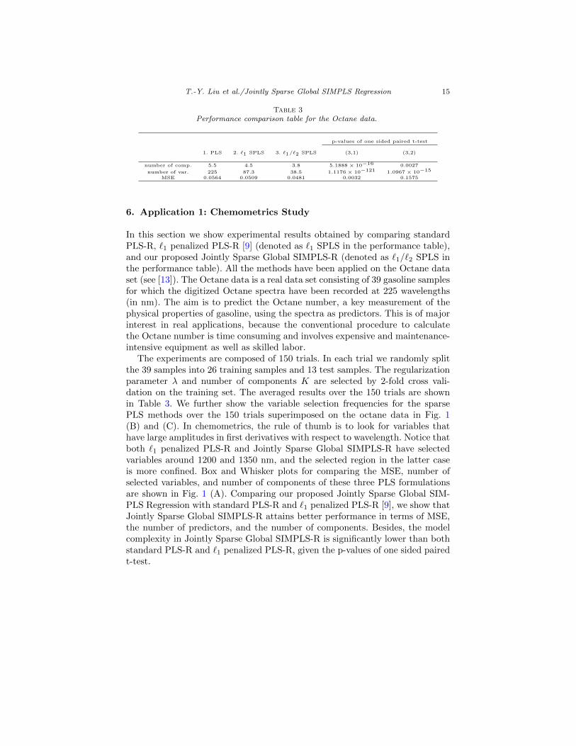
number of comp. 5.5 4.5 3.8 5.1888 × 10−16 0.0027

number of var. 225 87.3 38.5 1.1176 × 10−121 1.0967 × 10−15

MSE 0.0564 0.0509 0.0481 0.0032 0.1575

6. Application 1: Chemometrics Study

In this section we show experimental results obtained by comparing standardPLS-R, `1 penalized PLS-R [9] (denoted as `1 SPLS in the performance table),and our proposed Jointly Sparse Global SIMPLS-R (denoted as `1/`2 SPLS inthe performance table). All the methods have been applied on the Octane dataset (see [13]). The Octane data is a real data set consisting of 39 gasoline samplesfor which the digitized Octane spectra have been recorded at 225 wavelengths(in nm). The aim is to predict the Octane number, a key measurement of thephysical properties of gasoline, using the spectra as predictors. This is of majorinterest in real applications, because the conventional procedure to calculatethe Octane number is time consuming and involves expensive and maintenance-intensive equipment as well as skilled labor.

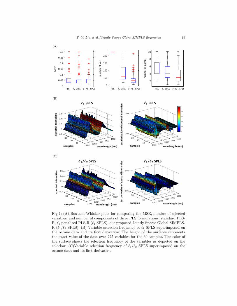
The experiments are composed of 150 trials. In each trial we randomly splitthe 39 samples into 26 training samples and 13 test samples. The regularizationparameter λ and number of components K are selected by 2-fold cross vali-dation on the training set. The averaged results over the 150 trials are shownin Table 3. We further show the variable selection frequencies for the sparsePLS methods over the 150 trials superimposed on the octane data in Fig. 1(B) and (C). In chemometrics, the rule of thumb is to look for variables thathave large amplitudes in first derivatives with respect to wavelength. Notice thatboth `1 penalized PLS-R and Jointly Sparse Global SIMPLS-R have selectedvariables around 1200 and 1350 nm, and the selected region in the latter caseis more confined. Box and Whisker plots for comparing the MSE, number ofselected variables, and number of components of these three PLS formulationsare shown in Fig. 1 (A). Comparing our proposed Jointly Sparse Global SIM-PLS Regression with standard PLS-R and `1 penalized PLS-R [9], we show thatJointly Sparse Global SIMPLS-R attains better performance in terms of MSE,the number of predictors, and the number of components. Besides, the modelcomplexity in Jointly Sparse Global SIMPLS-R is significantly lower than bothstandard PLS-R and `1 penalized PLS-R, given the p-values of one sided pairedt-test.


(A)

0

0.05

0.1

0.15

0.2

0.25

0.3

PLS L1 SPLSL1/L2 SPLS

MS

E

PLS ℓ1 SPLS ℓ1/ℓ2 SPLS0

50

100

150

200


num

ber o

f var

.

PLS ℓ1 SPLS ℓ1/ℓ2 SPLS

2

4

6

8

10


num

ber o

f com

p.

PLS ℓ1 SPLS ℓ1/ℓ2 SPLS

(B)

11021202

13021402

1502

1020

30

-0.2

0

0.2

0.4

0.6

wavelength (nm)

L1 SPLS

samples

spec

tral i

nten

sitie

s

ℓ𝟏𝟏 SPLS

11021202

13021402

1502

1020

30

-0.05

0

0.05

wavelength (nm)

L1 SPLS

samples 1s

t der

ivat

ive

of s

pect

ral i

nten

sitie

s

0

0.2

0.4

0.6

0.8

1

ℓ𝟏𝟏 SPLS

(C)

11021202

13021402

1502

1020

30

-0.2

0

0.2

0.4

0.6

wavelength (nm)

L1/L2 SPLS

samples

spec

tral i

nten

sitie

s

ℓ𝟏𝟏/ℓ𝟐𝟐 SPLS

11021202

13021402

1502

1020

30

-0.05

0

0.05

wavelength (nm)

L1/L2 SPLS

samples 1s

t der

ivat

ive

of s

pect

ral i

nten

sitie

s ℓ𝟏𝟏/ℓ𝟐𝟐 SPLS

Fig 1: (A) Box and Whisker plots for comparing the MSE, number of selectedvariables, and number of components of three PLS formulations: standard PLS-R, `1 penalized PLS-R (`1 SPLS), our proposed Jointly Sparse Global SIMPLS-R (`1/`2 SPLS). (B) Variable selection frequency of `1 SPLS superimposed onthe octane data and its first derivative: The height of the surfaces representsthe exact value of the data over 225 variables for the 39 samples. The color ofthe surface shows the selection frequency of the variables as depicted on thecolorbar. (C)Variable selection frequency of `1/`2 SPLS superimposed on theoctane data and its first derivative.


7. Application 2: Sparse Prediction of Disease Symptoms fromGene Expression

In this section we apply the Jointly Sparse Global SIMPLS Regression to 4types of predictive health challenge studies involving the H3N2, the H1N1, theHRV, and the RSV viruses. In these challenge studies, publicly available fromthe NCBI-GEO website, serial peripheral blood samples were acquired from apopulation of subjects inoculated with live flu viruses [38, 39, 40, 41]. The pre-diction task in these experiments is to predict the symptom scores based ongene expression of 12023 genes. There were 10 symptom scores, i.e., runny nose,stuffy nose, sneezing, sore throat, earache, malaise, cough, shortness of breath,headache, and myalgia, documented over time. The symptoms are self-reportedscores, ranging from 0 to 3. We linearly interpolate the gene expressions tomatch them with the sampling time of the symptom reports. We compare theJointly Sparse Global SIMPLS-R with standard PLS-R and `1 penalized PLS-Rby leaving one subject out as the test set, and the rest as the training set. Theprocess is repeated until all subjects have been treated as the test set. The num-ber of components for all methods and the regularization parameter in JointlySparse Global SIMPLS-R are selected by 2-fold cross validation to minimizethe sum of the MSE of the responses. Since each subject has multiple samples,we perform the cross validation by splitting by subjects, i.e., no samples fromthe same subject will appear in both training and tuning sets. We restrict theresponses to the first 3 symptoms, which are the upper respiratory symptoms,and the results are shown in Table 4. In most of the cases, the proposed JointlySparse Global SIMPLS-R method outperforms the standard PLS-R and `1 pe-nalized PLS-R in terms of prediction MSE, number of components, number ofgenes. As can be seen in Table 4, the number of selected variables decreasessignificantly by applying the `1/`2 mixed norm sparsity penalty to the PLS-R objective function. Thus the proposed PLS-R method is able to construct amore parsimonious predictor relative to the other PLS-R methods having similaraccuracy.

The PLS-R method can also be viewed as an exploratory data analysis toolfor constructing low dimensional descriptors of the independent variables and re-sponse variables. Specifically, the general underlying matrix factorization modelX = TP ′ + E and Y = TQ′ + F , with latent component T = XW , providesa factor analysis model for the independent and response variables X and Y .T , P and Q can be interpreted in a similar manner as the singular vectors ofPCA. However, different from PCA that does not account for the response vari-ables, T , P and Q contain information about both the independent variablesand the response variables. The factor analysis interpretation of the underlyingPLS model is that T is a latent score matrix and P , Q are latent factor load-ing matrices that associate T with the independent variables and the responsevariables via the approximate matrix factorizations X ≈ TP ′ and Y ≈ TQ′,respectively. The correlations between the latent component T and the sum ofthe 3 upper respiratory symptoms are reported in Table 5, which also showsresults for classic matrix factorization methods including non-negative matrix


Table 4Performance comparison table for the predictive health study. We apply the Jointly SparseGlobal SIMPLS Regression (`1/`2 SPLS) for sparse prediction of disease symptoms from

gene expression. The performance is compared with standard PLS and `1 sparse PLS. `1/`2SPLS achieves lower MSE with significantly fewer variables in most of the studies.

p-values of one sided paired t-test

1. PLS 2. `1 SPLS 3. `1/`2 SPLS (3,1) (3,2)

H1N1number of comp. 2.8 2.3 2.4 0.1163 0.3322

number of genes 12023 3624.1 3575.8 1.4451 × 10−10 0.4842Overall MSE 0.599 0.603 0.591 0.2890 0.1094

Runny nose MSE 0.167 0.165 0.167Stuffy nose MSE 0.281 0.282 0.269Sneezing MSE 0.151 0.157 0.155

H3N2number of comp. 3.2 2.5 1.9 0.0030 0.0863



HRVnumber of comp. 2.8 2.3 2.2 0.0484 0.3773



RSVnumber of comp. 3.2 2.3 2.4 0.0198 0.4103



factorization (NMF) [42] and Bayesian linear unmixing (BLU) [43, 44], previ-ously applied to this dataset, for comparison. Notice the sparse PLS-R meth-ods achieve higher correlation, as expected. Remarkably, the proposed JointlySparse global SIMPLS-R achieves this higher degree of correlation with manyfewer components and variables than the NMF and BLU methods. This ex-periment demonstrates that Jointly Sparse Global SIMPLS-R can be used as afactor analysis method to find the hidden molecular factors that best relate tothe response.

8. Conclusion

The formulation of the global SIMPLS objective function with an added groupsparsity penalty greatly reduces the number of variables used to predict theresponse. This suggests that when multiple components are desired, the vari-able selection technique should take into account the sparsity structure for thesame variables among all the components. Our proposed Jointly Sparse GlobalSIMPLS Regression algorithm is able to achieve as good or better performancewith fewer predictor variables and fewer components as compared to compet-ing methods. It is thus useful for performing dimension reduction and variable


Table 5Matrix factorization. We use the cross-validated parameters reported in Table 4 for standard

PLS-R and `1 penalized PLS-R, and the Jointly Sparse Global SIMPLS-R to decide thenumber of components, and search over the grid {1, 2, ..., 10} to find the number of factors

that achieves the highest correlation for NMF and BLU. The correlation between each factorand the sum of responses is listed for each method. The first 3 methods, PLS, `1 SPLS, and`1/`2 SPLS are supervised matrix factorizations, where as NMF and BLU are unsupervised.

The unsupervised methods require many more factors to achieve comparable correlation.

correlation of each factor with the sum of upper respiratory symptomsfactor 1 2 3 4 5 6 7 8 9

H1N1PLS 0.47 0.38 0.38

`1 SPLS 0.52 0.37`1/`2 SPLS 0.57 0.35

NMF 0.32 0.45 0.04BLU 0.27 0.19 0.02 0.51 0.16 0.06

H3N2PLS 0.67 0.42 0.33

`1 SPLS 0.73 0.33 0.33`1/L2 SPLS 0.71 0.33

NMF 0.62 0.70 0.10BLU 0.54 0.73 0.26 0.33 0.01 0.02 0.28 0.05 0.00

HRVPLS 0.45 0.43 0.35

`1 SPLS 0.52 0.38`1/`2 SPLS 0.53 0.42

NMF 0.02 0.22 0.19BLU 0.11 0.04 0.18 0.33 0.01 0.02 0.28 0.05 0.00

RSVPLS 0.66 0.35 0.35

`1 SPLS 0.70 0.34`1/`2 SPLS 0.69 0.39

NMF 0.41 0.13 0.16 0.01 0.31 0.02 0.11 0.11 0.01BLU 0.01 0.02 0.23 0.20 0.03 0.68 0.12


selection simultaneously in applications with large dimensional data but com-paratively few samples (n < p).

The Jointly Sparse Global SIMPLS Regression objective function is mini-mized using augmented Lagrangian techniques and, in particular, the ADMM al-gorithm. The ADMM algorithm splits the optimization into an eigen-decompositionproblem and a soft-thresholding that enforces sparsity constraints. The generalframework is extendable to more complicated regularization and can thus betailored for other PLS-type applications, e.g., positivity constraints or smooth-ness penalties. For example, in the chemometric application, the data is smoothover the wavelengths and we can apply wavelet shrinkage on the data or in-clude a total variation regularization to encourage smoothness. The sparsityconstraints can be imposed on the wavelet coefficients if wavelet shrinkage isapplied, or together with total variation regularization. The equivalence of softwavelet shrinkage and total variation regularization was discussed in [45]. Onecan also consider imposing sparsity structures on the weights corresponding tothe same components, adding `1 penalty within the groups, or total variationregularization, depending on the applications. The decoupling property of theADMM algorithm allows one to extend the Jointly Sparse Global SIMPLS Re-gression to these various regularizations.

References

[1] Wold, S., Martens, H., and Wold, H. (1983). The multivariate calibrationproblem in chemistry solved by the PLS method. Proceedings of the Confer-ence on Matrix Pencils. Lectures Notes in Mathematics, 286-293.

[2] Sjostrom, M., and Wold, S., and Lindberg, W., and Persson, J., and Martens,H. (1983). A multivariate calibration problem in analytical chemistry solvedby partial least-squares models in latent variables. Analytica Chimica Acta150, 61-70.

[3] Martens, H., and Martens, M. (1999). Validation of PLS Regression modelsin sensory science by extended cross-validation. PLS’99.

[4] Rossouw, D., Robert-Granie, C., and Besse, P. (2008). A sparse PLS for vari-able selection when integrating omics data. Genetics and Molecular Biology,7(1), 35.

[5] Chun, H., and Keles, S. (2009). Expression quantitative trait loci mappingwith multivariate sparse partial least squares regression. Genetics, 182(1),79-90.

[6] Chung, D., and Keles, S. (2010). Sparse partial least squares classificationfor high dimensional data. Statistical applications in genetics and molecularbiology, 9(1), 17.

[7] Chun, H., Ballard, D. H., Cho, J., and Zhao, H. (2011). Identification ofassociation between disease and multiple markers via sparse partial leastsquares regression. Genetic epidemiology, 35(6), 479-486.

[8] Wold, S., Ruhe, A., Wold, H., and Dunn III, W. J. (1984). The collinearityproblem in linear regression. The partial least squares (PLS) approach to


generalized inverses. SIAM Journal on Scientific and Statistical Computing,5(3), 735-743.

[9] Chun, H., and Keles, S. (2010). Sparse partial least squares regression for si-multaneous dimension reduction and variable selection. Journal of the RoyalStatistical Society: Series B (Statistical Methodology), 72, 3-25.

[10] de Jong, S. (1993). SIMPLS: an alternative approach to partial least squaresregression. Chemometrics and Intelligent Laboratory Systems, 18(3), 251-263.

[11] Wold, H. (1966). Nonlinear estimation by iterative least squares procedures.Research papers in statistics, 411-444.

[12] Hotelling, H. (1933). Analysis of a complex of statistical variables intoprincipal components. Journal of educational psychology, 24(6), 417.

[13] Tenenhaus, M. (1998). La Regression PLS: theorie et pratique. EditionsTechnip.

[14] de Jong, S. (1995). PLS shrinks. Journal of Chemometrics, 9(4), 323-326.[15] Boulesteix, A. L., and Strimmer, K. (2007). Partial least squares: a ver-

satile tool for the analysis of high-dimensional genomic data. Briefings inbioinformatics, 8(1), 32-44.

[16] Hoskuldsson, A. (1988). PLS regression methods. Journal of Chemometrics,2(3), 211-228.

[17] ter Braak, C. J., and de Jong, S. (1998). The objective function of partialleast squares regression. Journal of chemometrics, 12(1), 41-54.

[18] Jolliffe, I. T., Trendafilov, N. T., and Uddin, M. (2003). A modified principalcomponent technique based on the LASSO. Journal of Computational andGraphical Statistics, 12(3), 531-547.

[19] Wold, H. (1975). Soft modelling by latent variables: the non-linear iterativepartial least squares (NIPALS) approach. Perspectives in Probability andStatistics, In Honor of MS Bartlett, 117-144.

[20] Allen, G. I., Peterson, C., Vannucci, M., and Maletic-Savatic, M. (2013).Regularized partial least squares with an application to NMR spectroscopy.Statistical Analysis and Data Mining, 6(4), 302-314.

[21] Bach, F. R. (2008). Consistency of the group Lasso and multiple kernellearning. The Journal of Machine Learning Research, 9, 1179-1225.

[22] Gander, W. (1980). Least squares with a quadratic constraint. NumerischeMathematik, 36(3), 291-307.

[23] Gander, W., Golub, G. H., and von Matt, U. (1989). A constrained eigen-value problem. Linear Algebra and its applications, 114, 815-839.

[24] Beck, A., Ben-Tal, A., and Teboulle, M. (2006). Finding a global optimalsolution for a quadratically constrained fractional quadratic problem withapplications to the regularized total least squares. SIAM Journal on MatrixAnalysis and Applications, 28(2), 425-445.

[25] Eckstein, J., and Bertsekas, D. P. (1992). On the Douglas-Rachford splittingmethod and the proximal point algorithm for maximal monotone operators.Mathematical Programming, 55(1-3), 293-318.

[26] Goldstein, T., and Osher, S. (2009). The split Bregman method for L1-regularized problems. SIAM Journal on Imaging Sciences, 2(2), 323-343.


[27] Afonso, M. V., Bioucas-Dias, J. M., and Figueiredo, M. A. (2011). An aug-mented Lagrangian approach to the constrained optimization formulation ofimaging inverse problems. Image Processing, IEEE Transactions on, 20(3),681-695.

[28] Boyd, S., Parikh, N., Chu, E., Peleato, B., and Eckstein, J. (2011). Dis-tributed optimization and statistical learning via the alternating directionmethod of multipliers. Foundations and Trends R© in Machine Learning, 3(1),1-122.

[29] Hong, M., and Luo, Z. Q. (2012). On the linear convergence of the alter-nating direction method of multipliers. arXiv preprint arXiv:1208.3922.

[30] Goldstein, T., O’Donoghue, B., and Setzer, S. (2012). Fast alternating di-rection optimization methods. CAM report, 12-35.

[31] Ramani, S., and Fessler, J. A. (2012) A splitting-based iterative algorithmfor accelerated statistical X-ray CT reconstruction. Medical Imaging, IEEETransactions on, 31(3), 677-688.

[32] Nien, H., and Fessler, J. A. (2014). A convergence proof of the splitBregman method for regularized least-squares problems. arXiv preprintarXiv:1402.4371.

[33] Bair, E., Hastie, T., Paul, D., and Tibshirani, R. (2006). Prediction bysupervised principal components. Journal of the American Statistical Asso-ciation, 101(473).

[34] Bastien, P., Vinzi, V. E., and Tenenhaus, M. (2005). PLS generalised linearregression. Computational Statistics & Data Analysis, 48(1), 17-46.

[35] Tibshirani, R. (1996). Regression shrinkage and selection via the lasso.Journal of the Royal Statistical Society. Series B (Methodological), 267-288.

[36] Martens, H., and Naes, T. (1989). Multivariate calibration. Wiley.[37] Masoum, S., Bouveresse, D. J. R., Vercauteren, J., Jalali-Heravi, M., and

Rutledge, D. N. (2006). Discrimination of wines based on 2D NMR spectrausing learning vector quantization neural networks and partial least squaresdiscriminant analysis. Analytica chimica acta, 558(1), 144-149.

[38] Zaas, A. K., Chen, M., Varkey, J., Veldman, T., Hero, A. O., Lucas, J.,Huang, Y., Turner, R., Gilbert, A., Lambkin-Williams, R., Øien, N. C.,Nicholson, B., Kingsmore, S., Carin, L., Woods, C. W., and Ginsburg, G.S. (2009). Gene Expression Signatures Diagnose Influenza and Other Symp-tomatic Respiratory Viral Infections in Humans. Cell Host and Microbe,6(3), 207-217.

[39] Huang, Y., Zaas, A. K., Rao, A., Dobigeon, N., Woolf, P. J., Veldman,T., Øien, N. C., McClain, M. T., Varkey, J. B., Nicholson, B., Carin, L.,Kingsmore, S., Woods, C. W., Ginsburg, G. S., Hero, A. O. (2011). Tem-poral dynamics of host molecular responses differentiate symptomatic andasymptomatic influenza a infection. PLoS genetics, 7(8), e1002234.

[40] Woods., C. W., McClain, M. T., Chen, M., Zaas, A. K., Nicholson, B. P.,Varkey, J., Veldman, T., Kingsmore, S. F., Huang, Y., Lambkin-Williams,R., Gilbert, A. G., Hero, A. O., Ramsburg, E., Glickman, S., Lucas1, J. E.,Carin, L., and Ginsburg, G. S. (2013). A host transcriptional signature forpresymptomatic detection of infection in humans exposed to influenza H1N1


or H3N2. PloS one 8.1: e52198.[41] Zaas, A. K., Burke, T., Chen, M., McClain, M., Nicholson, B., Veldman, T.,

Tsalik, E. L., Fowler, V., Rivers, E. P., Otero, R., Kingsmore, S. F., Voora,D., Lucas, J., Hero, A. O., Carin, L., Woods, C. W., and Ginsburg, G. S.(2013). A Host-Based RT-PCR Gene Expression Signature to Identify AcuteRespiratory Viral Infection. Science translational medicine, 5, 203ra126.

[42] Paatero, P., Tapper, U. (1994). Positive matrix factorization: A non-negative factor model with optimal utilization of error estimates of datavalues. Environmetrics, 5(2), 111-126.

[43] Dobigeon, N., Moussaoui, S., Coulon, M., Tourneret, J. Y., and Hero, A.O. (2009). Joint Bayesian endmember extraction and linear unmixing forhyperspectral imagery. Signal Processing, IEEE Transactions on, 57(11),4355-4368.

[44] Bazot, C., Dobigeon, N., Tourneret, J.-Y., Zaas, A. K., Ginsburg, G. S. ,Hero, A. O. (2013). Unsupervised Bayesian linear unmixing of gene expres-sion microarrays. BMC Bioinformatics, 14(1), 99.

[45] Steidl, G., Weickert, J., Brox, T., Mrzek, P., and Welk, M. (2004). On theequivalence of soft wavelet shrinkage, total variation diffusion, total variationregularization, and SIDEs. SIAM Journal on Numerical Analysis, 42(2),686-713.

jointly sparse global simpls regression - arxiv · jointly sparse global simpls regression tzu-yu...

Documents