joint p- and s-wave velocity reﬂection tomography using pp

CWP-473P

Joint P- and S-wave velocity reflection tomography using PPand PS data: An approach based on co-depthing anddifferential semblance in scattering angle optimization

Stig-Kyrre Foss�, Bjørn Ursin

�, and Maarten V. de Hoop ��

Department of Mathematical Sciences, NTNU, N-7491 Trondheim, Norway�Department of Petroleum Engineering and Applied Geophysics, NTNU, N-7491 Trondheim, Norway�Center for Wave Phenomena, Colorado School of Mines, Golden CO, USA

1st April 2004

ABSTRACTThe velocity-depth ambiguity in depth migration is a well known problem stemmingfrom several factors, such as limited aperture, band-limitation of the source and theinterplay between parameters of the background medium contributing to the non-uniqueness of the problem. In addition, the isotropic assumption can cause severedepth errors in the presence of anisotropy. These are severe issues when consider-ing PP and PS images from depth migration where geologically equivalent horizonsshould be mapped to the same depths. The present method is based upon the differ-ential semblance misfit function in angle to find fitting background models. This re-quires amplitude-compensated angle-domain common image-point gathers to be uni-form. Depth consistency between the PP and PS depth image is enforced through aregularization approach penalizing mistie between key imaged reflectors in addition tothe differential semblance misfit function. By migration/map demigration, time infor-mation is obtained on the key reflectors of the PP and PS image. This time information,which is independent of the velocity model, can be map-migrated to reconstruct the re-flectors in depth for a given background model giving an automatic way to quantifythe depth discrepancy in the tomographic approach. An approximative simplificationuses the normal-incidence point rays in the map migration. The method is presented ina general 3-D framework allowing for the use of true depth information such as wellmarkers and the inclusion of anisotropy. A strategy is presented to retrieve all parame-ters of a transversly isotropic medium with a known symmetry axis depending on theavailable information. This is employed on an ocean bottom seismic field data set fromthe North Sea.

Key words: Reflection tomography, generalized Radon transform, differential sem-blance in angle, anisotropy, converted waves.

1 INTRODUCTION

Here, we demonstrate the use of annihilator-based migrationvelocity analysis (MVA), related to the differential semblance(Symes and Carazzone, 1991) approach, on joint PP and PS re-flection data. The misfit function associated with this approachis unique in that it depends smoothly on the velocity model. Asis common in MVA we model the reflection data in the singlescattering approximation, yielding a forward scattering opera-tor that, given a velocity model, maps reflectors to reflections.

By a gradient-based search of the model space, the range ofthe forward scattering operator is adapted to contain the data.Data are in the range if they can be predicted by the operator.

Annihilators detect whether the data are in the range ofthe forward scattering operator (Stolk and de Hoop, 2002).They have their counterpart in the image domain: The dataare in the range if the common image-point gathers (CIGs)obtained from the data – parametrized by scattering angle andazimuth – are uniform, i.e., flat and show angle-independentamplitude; annihilators emerge as derivatives with angle.

144 S-K. Foss, B. Ursin & M.V. de Hoop

As MVA typically is based on a small collection of reflec-tions, one expects an inherent non-uniqueness in the inverseproblem of determining the velocity model. We consider a ve-locity model to be acceptable if the reflections are in the rangeof the forward scattering operator. In this paper, we search inthe class of acceptable velocity models for a model that notonly predicts the PP and PS reflections in time, but also tiesthe PP and PS images of corresponding reflectors in depth. Inthis so-called co-depthing process, one needs to ensure thatthe PP and PS images indeed have these reflectors in common,which requires a degree of seismic interpretation. Co-depthingcan also be carried out with well data.

Tradionally, MVA exploits the redundancy in the data bystudying the residual moveout on CIGs (Al-Yahya, 1989). Flatgathers guarantee a velocity model resulting in a well-focused(sharp) image. Image gathers are formed from data subsets,typically parametrized by offset. The differential semblancemisfit function (Symes and Carazzone, 1991) measures theresidual moveout on these CIGs and quantifies the degree of fitbetween traces by a local derivative in offset. This procedurehas been carried out by Plessix et al. (2000) and Chauris andNoble (2001) amongst others.

In the presence of caustics, an image generated fromcommon-offset data will, however, contain artifacts (falsereflectors). To remedy this, (surface) offset and azimuth,parametrizing data subsets, have been replaced by the (subsur-face) scattering angle and azimuth between in- and out-goingrays at the image point. In the Kirchhoff approach to seismicinverse scattering it has been proposed to use a generalizedRadon transform (GRT) to generate a set of images parame-terized by these angles (de Hoop et al., 1994; de Hoop et al.,1999). The GRT, here, is derived from a least-squares data-fitting formulation of the inverse scattering problem. Artifactsdue to the formation of caustics are suppressed by a ‘focusingin dip’ procedure (Brandsberg-Dahl et al., 2003a), using onlythe contributions to the diffraction integral that are close tothe specular reflections. Such artifacts were numerically stud-ied by Brandsberg-Dahl et al. (2003a) and analyzed by Stolk(2002). Annihilators appear in the image domain, essentiallyas local derivatives with angle of CIGs, see Brandsberg-Dahlet al. (1991; 2003b), thus forming a differential semblancemeasure from CIGs in angle rather than offset; this approachhas been applied to a field case study by Foss et al. (2003b).

In the absence of caustics, the differential semblancemeasure seems to yield a global minimizer (Symes, 1991).This means that the initial velocity model can be quite far froman acceptable model, and optimization will still result in suchan acceptable model. Numerical experiments carried out byPlessix et al. (2000) suggest using differential semblance opti-mization until a certain rate of improvement and then switch-ing to semblance optimization (Taner and Koehler, 1969). Wefollow this suggestion only in those parts of the velocity modelwhere we fine tune our estimate of anisotropy.

To ensure that AVA behavior on the CIGs – associatedwith a reflection coefficient or contrast-source radiation pat-terns – does not contribute to the differential semblance in an-gle, one either has to adapt the definition of the annihilator

(Foss et al., 2003a, (54-55)) or modify the amplitude func-tion in the GRT inverse (Brandsberg-Dahl et al., 2003b, (11)and below) to resolve one particular elastic parameter combi-nation. This combination is controlled by the contrast-sourceradiation patterns, and is illucidated in the main text of thispaper. We loosely refer to the resulting GRT as ‘amplitude-compensated migration’; the details of such a process can befound in Ursin (2003). It is noted that the calculation of radia-tion patterns does not make use of the medium perturbations,which is a consequence of the Born(-Kirchhoff) approxima-tion on which the migration procedure is based.

Several authors have recently approached the problem ofjoint PP and PS velocity analysis (Sollid, 2000; Stopin andEhinger, 2001; Alerini et al., 2002; Grechka and Tsvankin,2002b; Broto et al., 2002; Grechka and Tsvankin, 2002b;Broto et al., 2003); see Herrenschmidt et al. (2001) for areview. The diodic nature of PS reflections (Thomsen, 1999)demands a treatment of MVA different from that for PP reflec-tions. The diodic nature is a consequence of the fact that PS re-flections are non-reciprocal in source and receiver; indeed, thereciprocal of PS is SP. It is also a well-known difficulty that im-ages of a common geological reflector from PP and PS reflec-tions often do not match in depth. There are several reasons forthis. The velocity-depth ambiguity (Stork and Clayton, 1986;Bube, 1995; Bube al., 2002) is intimately connected to raycoverage and acquisition aperture. In addition, anisotropy hasto be included in order to compute depth-consistent PP andPS images because an isotropic assumption can cause severedepth errors in the presence of anisotropy Artola al., 2003).This applies especially to converted waves. And then, withan anisotropic medium, there is an added ambiguity in theinterplay between the different elastic parameters (Bube andMeadows, 1999). Versteeg (1993) showed how continuouslysmoothing a correct model would recreate the image geomet-rically, yet blur it. One can view these apparent ambiguitiesas structures in the manifold of acceptable velocity models,i.e., velocity models that recreate the data: The range of theforward scattering operator does not change significantly be-tween models in this manifold. The tying of PP and PS imagesof common reflectors constrains the manifold of acceptablevelocity models.

PP angle tomography by means of differential semblancein angle optimization Brandsberg-Dahl et al. (2003b) is hereextended to PS reflections, accounting for their diodic nature.The key contribution of this paper is a methodology of co-depthing the PP and PS CIGs in angle in the framework ofangle tomography. In practice, we focus the tying of PP andPS images in depth on prior chosen key reflectors that are pre-sumed to be the same based on geological grounds. To facil-itate the inclusion of other depth information, we introducethe notion of reference depth function. This function can bederived from well information, if available, or from strong,coherent reflectors on the PP image; a PP image usually hassuperior ray coverage and hence superior resolution.

To perform the tying in depth of the PP and PS reflec-tions, we use time horizons obtained from paired and pickedevents in depth on PP and PS images that are map-demigrated

Joint P and S velocity reflection tomography 145

to time. Using map migration (Kleyn, 1977; Gjoystdal andUrsin, 1981) of the time horizons for every suggested velocitymodel we are able to quantify the depth mismatch in an auto-matic way. Notice that the time horizons need only be pickedonce. Map (de)migration can be used in complex media; seeDouma and de Hoop (2003) for details and references. For theconverted-wave events the ability to perform PS map migra-tion is highly dependent on how close we are to the true modelinitially; hence we have opted for applying the ‘PP+PS=SS’approach of Grechka and Tsvankin (2002b) to convert PS toSS for this purpose. In this paper we use a zero-offset restric-tion by map demigrating normal incidence point (NIP) rays(Hubral and Krey, 1980) as suggested by Whitcombe (1994). For the mode converted waves we employ a simplified ver-sion of the ‘PP+PS=SS’ approach using NIP rays to computeapproximate zero-offset SS traveltime data.

The outline of the paper is as follows. In following sec-tion, we introduce notation and show how to transform datato CIGs in scattering angle and azimuth for the purpose ofvelocity analysis. The formulation here is in 3-D and followsthe presentation of Ursin (2003); the 2.5-D formulation andits subleties are presented in Foss et al. (2003a). Then wegive a brief review of PP angle tomography (Brandsberg-Dahlal., 2003b) and its extension to mode-converted waves. In thenext section, we introduce our co-depthing methodology in theframework of the differential semblance in angle optimizationby adding a penalizing term to the misfit function. Then wepresent a step-wise strategy using the aforementioned tomog-raphy tools to obtain values of a transversely isotropic (TI)medium with a known symmetry axis. Although the strategyis presented for a 3-D medium, we disregard the presenceof azimuthal anisotropy. Such a medium is equivalent to aTI medium with a vertical symmetry axis through the Bondtransformations (Carcione, 2001). It can be parameterized by�� , and

�. which are the vertical P- and S-wave ve-

locities and the Thomsen (1986) parameters, respectively. Theoptimization strategy is split into the following steps:

(i) isotropic P-wave velocity analysis on PP CIGs using dif-ferential semblance in angle;

(ii) isotropic S-wave velocity analysis on PS CIGs usingdifferential semblance in angle, making use of the P-wave ve-locity model obtained in (i);

(iii) seismic interpretation of the PP and PS images for keyreflectors; map demigration of these reflectors yielding timehorizons;

(iv) co-depthing of PP and PS images of key reflectors toobtain an optimal isotropic S-wave velocity model, using thedifferential semblance in angle of the PP and PS CIGs as reg-ularizer;

(v) differential semblance in angle and semblance opti-mization of PP and PS CIGs jointly allowing the model tobecome anisotropic, enforcing the depth consistency.

Several authors have discussed the point that, in order toobtain information on the

�parameter, one either needs infor-

mation of the true depth of a reflector through well logs or trav-eltimes from rays that have traveled at an oblique angle, e.g.,

from strongly dipping reflectors or from large-offset data (Au-debert et al., 2001; Iversen et al., 2000). In the absence of suchinformation, several approaches have been suggested (Alkhali-fah and Tsvankin, 1995; Grechka and Tsvankin, 2002b). Here,we make the convenient choice of setting

�equal to zero con-

sidering a quasi-TIV medium. The remaining parameter isnot the true anisotropy parameter, but an effective one.

Finally, we employ the above methodology on a NorthSea ocean bottom seismic (OBS) field data set to obtain firsta quasi-TIV velocity model and then all parameters of a TIVvelocity model.

2 MIGRATION TO ‘UNIFORM’ ANGLE COMMONIMAGE-POINT GATHERS

Dip, scattering angle, and azimuth. We consider migrationof seismic data in a 3-D heterogeneous anisotropic elasticmedium. The geometry is shown in Figure 1 where the im-age point is denoted by �� . Source positions inthe acquisition manifold are denoted by �� and receiver po-sitions by �� (bold fonts indicate vectors). The superscripts �and indicate association with a ray from a source and a re-ceiver, respectively. The covector !"�#�� $� is the slowness vec-tor of the ray connecting the source point � � with the imagepoint evaluated at the latter point; ! � �� indicates the slow-ness along this ray evaluated at the source. It is the projection% � �� of ! � �� on the acquisition manifold that is detected(via slope estimates) in the data. We furthermore introduce thephase direction & � �'! �)(+* ! ��* and the phase velocity � � ac-cording to * ! � * �-, ( � � . A similar notation is employed forthe slowness vector related quantities along the ray connect-ing the receiver with the image point, namely ! � �� $� , ! � �� ,and % � �� , as well as & � and � � . The polarization vector,.

, is defined in the same manner as that for the slowness vec-tor at the source, receiver and image point. The migration dip,/�0 �� $� , is the direction /�0 �� "�1! 0 �� $� (+* ! 0 �� $� * of the mi-gration slowness vector, ! 0 �� 2�3!$�#�� $��45!�� $� .

The scattering angle, 6 , between incoming and scatteredrays, is defined by

7)8:9 6;�1& �=< & � at 2>?6;�16�� (1)

for a particular diffraction branch away from caustics at � � or�@� . The scattering azimuth, A , is the angular displacement ofthe vector B (+* B * with

BC�D�E& �GF & � � F / 0 at H>IA5�3AG�� KJ (2)

The two-way traveltime for a particular diffraction branch as-sociated with a ray path connecting �� with �� via is de-noted by L1�MLN�� @�)� .

Map (de)migration. Map migration describes how thegeometry of a reflection is mapped on the geometry of a re-flector,OQP �� SRK�T% � �T% � �"UVW�� ! 0 � at R �3LN�� (3)

such that the normal to the reflector is given by /X0 . For agiven value of �E6 � A�� this process can be reversed to yield map


demigration,�P �� ! 0 � 6 � A��"UV �� LN�� T% � �T% � �KJ (4)

Map demigration corresponding to the exploding reflector model is obtained by setting 6X�� ; then the receivers (at zero offset,�@� �1�@� ) are connected with the reflectors via normal incidence point (NIP) rays (Hubral and Krey, 1980).

Generalized Radon transform inversion. The medium is described by its stiffness tensor �� ( � � �� , � J J �� ) anddensity � . These parameters are decomposed as a sum of a smooth part (with superscript �� ) and a perturbation (with superscript�S,�� ):� ��"�� 4�� "� � � �� @4�� KJ (5)

The estimation of the smooth part, the velocity model, is the objective of MVA while the medium perturbations contain anysingularities (reflectors) and are found by imaging-inversion, given a velocity model. We assume now that the perturbations arejumps in the parameters across a smooth interface defined by the zero level set !$��"� of a function ! (de Hoop and Bleistein,1997); multiple interfaces are simply treated with a finite collection of level-set functions. The interface normal is given by /$# �% ! (+* % ! * . Throughout we use the subscript summation convention.

In preparation of migration of seismic data to ‘uniform’ angle common image-point gathers, we consider the following formof the GRT, derived from the Born approximation,&')( �� H>T6 � A��"� *,+.-�/1032$45 �� * ! 0 �� $� * �76 / 0 � (6)

in which � � �1� � �� / 0 � 6 � A�� and � � �1� � �� / 0 � 6 � A�� , as illustrated in Figure 1. This transform is a stripped down version ofBrandsberg-Dahl al. (2003a, (20)) in as much as the radiation-pattern inversion has been removed as well as the contribution* ! 0 �� * ( � / 0 �� < / # �� $� � to the obliquity factor (Ursin, 2003). The domain of integration over / 0 is indicated by 8

- /�8

- /�E6 � A��:9 ' � and reveals the illumination or acquisition footprint. The data

45 corrected for amplitude, phase, and traveltime ata given image point are (Burridge et al., 1998, (4.2))45 �� "� ; �< �� 45 � � �<7= �� LN�� >; �= ��

<@?3A � � �� B � C � A DFEG)H � �� $� D3EG�H � �� B � CK� � (7)

where � � �� denotes the bulk density of the smooth background, while45 � � �<= denotes the multi-component data corrected for a possible

phase shift due to the presence of caustics,45 � � �<= �� LN�� "��IKJ � LNM$O PFO LRQ � 5 � � �<= �� LN�� KJ (8)

Here, I denotes the Hilbert transform (note that I � �TS;, ) while U2�� 2� V�� $�+4WV@�� is the accumulated KMAHindex for the ray connecting �� to the image point and the ray connecting the image point to �� . Furthermore, H ��@� � $� andH �� are the relative geometrical spreading (Cerveny, 2001) for the receiver and source rays, respectively. All factors thatenter in (6)-(7) are calculated with the aid of kinematic and dynamic ray tracing. Based on (de Hoop and Bleistein, 1997, (37-38)),the GRT in (6) is designed to reconstruct a distribution of the type' � � � �� 2>T6 � A�� /X# < ! 0 ��Y � * % P ! * � ��!$�� $� � �in which

' � � � is independent of ! 0 up to leading order asymptotics (though it does depend on / # ); ' � � � is strictly only defined for with !"�� "�Z� .

For given �� and �@� , let � # be the specular reflection point with associated dip /[# �� # � . For in the vicinity of this specularreflection point, we have

� /\# < ! 0 ��Y � * % P ! * � ��!$�� $� �^]C�`_ # ��Y � * % L ! * LNa � � % L ! * LNa < �� bS � # � �"�C�`_ # ��Y � � � /\# < �� bS � # � �where _ # is given by_ # � * ! 0 �� # � * such that / 0 ��

#�2� /^# �� # � � (9)

which is the so-called stretch factor (Tygel al., 1994; Ursin, 2003). We have

�`_ # ��Y � � � /\# < �� [S � # � �"� � �`_ # /^# < �� bS � # � �KJResolution analysis, assuming a band-limited signature common for all the sources, then leads to the factorization,&' ( �� H>T6 � A��"� &' � � � �� # >T6 � A��3c �`d�O e � �`_ # /X# < �� bS � # � � � * bS � # * small � (10)

where c � d@O e � denotes a �E6 � A�� -family of smooth functions revealing the acquisition footprint at � # (de Hoop and Bleistein, 1997,(94)).


AVA compensation. The relative contrast in the medium parameters is formally defined by the ‘vector’� � � � �� $�"� � � � � � �� $�� $� � � � � �� $�� $� � �� $�� J (11)

Its dimension depends on the symmetry of the elastic medium. For the PP and PS reflection problem in a TIV medium, which willbe treated in the field data example, it is of dimension 5. We have assumed that � � � � �� =�� !"�� with �� !$�� =�� !$�� $� � , where denotes the derivative with respect to the second argument, and

�denotes the local magnitude of the jump

across the zero level set of ! . Then (de Hoop and Bleistein, 1997, (38))' � � � �� # >T6 � A��"�� # � /^# � 6 � A�� # � � � �� # � /^# � 6 � A�� # � � (12)

where denotes the ‘vector’ of radiation patterns �� "��; �0 �� >; �0 �� A ; �� _ �� >; � � �� _ � �� B � �� $� � �� J (13)

Here, � �� and � �� are the phase velocities at averaged over phase angles. We refer to' � � � as linearized scattering coefficients;

&' � � �is a filtered realization of

' � � � , where the filter is determined by the illumination.For the estimation of the smoothly varying parameters of the background medium (velocity model) we use a slight modification

of transform (6), with� �� H> 6 � A�� P � * +.-�/ 0 2 45 �� * ! 0 �� $� * �* +�� * 6 / 0 � (14)

* �� @� � * is the Euclidean norm of the ‘vector’ of radiation patterns. At specular reflection points,' � � � in (12) gets replaced by� �� # > 6 � A��

#� with � �� # > 6 � A��2� �� # � /\# � 6 � A�� # � �@�:�� # � /\# � 6 � A��

* �� # � /\# � 6 � A�� # � � � �� # � /\# � 6 � A�� * JWe anticipate that � is only weakly dependent on �E6 � A�� ; hence, Ursin (2003) refers to (14) as amplitude-compensated migration.

For interpretation and comparisons, we also use the structural image,� �� $�2� * * � �� H> 6 � A�� 6 6 6 A J (15)

Subscripts are used to indicate whether a current common image-point gather (14) or structural image (15) is computed from PP orPS reflections:

� �� and� �� , respectively.

In the presence of caustics,� �� H>T6 � A�� as defined in (14) commonly generates artifacts. A remedy for this is the use of the

downward continuation approach from which an angle transform can be extracted that generates CIGs in angle without artifacts(Stolk and de Hoop, 2004). In the field case study in this paper, we believe that the formation of caustics plays a minor role; thecomplexity here arises from the elasticity.

3 ANGLE REFLECTION TOMOGRAPHY BY OPTIMIZATION

Tomography is performed to estimate the parameters describing the smooth part of the medium in equation (5) by kinematicand dynamic ray tracing, to compute the different quantities and factors in (7). The parameters are the density at the sourcesand receivers and the elastic stiffness tensor in the subsurface. For an isotropic background medium, only the P-wave velocity isrequired for a P-wave mode and only the S-wave velocity for an S-wave mode. Each parameter is given a representation with afinite number of coefficients, defining a finite-dimensional subspace of velocity models. If we assume that � coefficients, denoted by� �C�� J)J)J � �� , are sufficient to describe the background medium, the CIGs generated by (14) are denoted by

� �� >T6 � A�� .The differential semblance in angle misfit function Symes and Carazzone, 1991; Brandsberg-Dahl et al., 2003b) for PP reflec-

tions is given by� �@� � � �"� ,? * * * * 0 d�O e � �� > 6 � A�� * ��6 6 6 A 6 HJ (16)

A minimum of this function is found for uniform gathers; uniform gathers guarantee optimal focusing of the structural image. Themisfit function can be minimized by a gradient-based search of the model space such as a quasi-Newton method (Gill et al., 1981).

In setting up the optimization, one has to decide which quantities are kept fixed under perturbation of the velocity model inbetween the reflector and the acquisition manifold: �� ! 0 � 6 � A�� or �� SR � % � �T% � � . We will keep the first set of variables fixedin the present approach. A component of the gradient of the misfit function (16) is then given by (Brandsberg-Dahl al., 2003b)0 � �@� � � �0 � � �

* * *�0 d�O e � �@� �� >T6 � A�� 0�0 d@O e � �@� �� > 6 � A��0 � � 6 6 6 A 6 HJ (17)


A perturbation of the velocity model thus implies a per-turbation of mapping

�, illustrated in Figure 2. The deriva-

tive of the CIGs with the medium parameters can be evaluatedwith the aid of ray perturbation theory (Farra and Madariaga,1987; Cerveny, 2001) and can be found in Brandsberg-Dahl etal. (2003b, (12)). Motivated by a study of Symes (2000), weconjecture that the minimum of our misfit functions can be ob-tained by optimization even with poor starting values for thebackground medium parameters.

PS angle tomography. Due to the diodic nature (Thom-sen, 1999) of the PS reflections, we split the CIGs contributingto the misfit function into positive and negative constituents,denoted by

��@� and� Y�� . In the absence of caustics the pos-

itive constituents are formed from positive acquisition offsetdata whereas the negative constituents are formed from nega-tive acquisition offset data: The

�� CIGs are generated fromseismic events where the source and receiver rays intersect atthe image point with orientations shown in Figure 3. The split-ting is necessary in a tomographic procedure because the raysfor the two constituents travel in different parts of the velocitymodel. The complete misfit function is, hence, given by� �� "� ,? * * * � * 0 d@O e � �� >S6 � A�� * �

4 *0 d�O e � Y�� > 6 � A�� * � � 6 6 6 A 6 2J (18)

4 CO-DEPTHING THE PP AND PS IMAGES

Since the GRT approach is based upon a high-frequency ap-proximation and decouples S- from P-wave propagation, weneed to consider possible inconsistency in depth of reflectorscommon in PP and PS images. In reflection tomography wetherefore incorporate a term in the misfit function that penal-izes mismatch in depth of a small collection of key reflectors.A key reflector in the structural images is chosen on the basisof the following criteria: (i) coherency, and (ii) focusing. Thena key reflector is easily picked. We emphasize that finding thekey reflectors requires a degree of seismic interpretation. Thedifficulty here is assuring that the PP and PS imaged reflectorspertain to the same geological interface.

Let the � ’th pair of interpreted key reflectors on depth-migrated PP and PS images be given by the graphs� �� @� �� > � � � � �� > � � � � (19)

for a given velocity model � . Matching these interfaces indepth can be performed by velocity-model updating, each timecarrying out the migration on PP and PS data, and performingthe interpretation. The key reflectors on the PP and PS imagescan also be matched to their depths �� ( �� derived fromwell logs at well locations �� .

To include the co-depthing in our MVA procedure with-out performing full (GRT) migrations repeatedly in the scan-ning procedure above, we suggest following a map migrationapproach instead. The small collection of picked key reflec-tors, yielding position of and normal to each of them, frommigrated images (19) are map demigrated into PP and PS re-

flection time surfaces and slopes (Kleyn, 1977). This informa-tion is now considered as data.

For variable velocity models, we subject the reflectiontime surfaces and slopes to map migration, reconstructing thekey interfaces in depth and thus enabling a geometrical com-parison. It seems, however, that we have introduced an am-biguity: The continuation of the GRT with velocity is basedon keeping the input variables to map demigration (

�in (4))

fixed, while the continuation of the co-depthing is based onkeeping the input variables to map migration (

Oin (3)) fixed.

We come back to this in the next section on strategy. The flowof the image points with changing velocity model coincideswith so-called velocity rays (Fomel, 1997).

As an approximation, here, we restrict the above men-tioned matching procedure to zero scattering angle, i.e.,exploding-reflector model data; then only normal-incidencepoint (NIP) rays to the surface (Hubral and Krey, 1980) areto be accounted for. Special consideration is needed for theconverted-wave case with its diodic. We expose that below.

PURE-MODE EVENTS

Map demigration. Indicated in Figure 4 are two NIP rays forthe reflector point for two different wave modes, P wavesand S waves. The NIP ray for the PP reflection connects �and , and for the SS reflection � and ; the two-way NIPray traveltimes are � �� and � � � �� , respectively. Eventhough the rays of the two wave modes both take off normal tothe interface, they usually follow different paths to the surface,as indicated. The PP and SS NIP rays coincide only when the�� ( �� -ratio is constant throughout the velocity model.

Map migration. Using map migration in a given back-ground medium � , we map the time horizons and slopes todepth horizons and dips. A particular imaged reflector point iswritten as �� #> � � � � �� T%�� ; see Fig-ure 5. Also indicated in the figure is the imaged key reflec-tor point given a different model � . The arrow indicates themovement of image points and dips along the velocity ray.Note that, in principle, the process of repeated map migrationsdoes not require that the images of a key reflector have to bepicked again after each velocity model update.

Converted-mode events

We shall employ a simplification of and approximation to the‘PP+PS=SS’ approach of Grechka and Tsvankin (2002b). Theamplitude of a PS event at zero scattering angle vanishes. Nev-ertheless, in the PS angle gathers we can extrapolate the sin-gular supports to zero angle.

In an acceptable velocity model for the PS event, the NIP-P ray connects to � and the NIP-S ray connects to � as inFigure 4. The two-way traveltime is then given by,

� �� "�� ( ? 4 � � � �� ( ? � (20)

with reflection point . Notice the use of two arguments inthe traveltime function for converted modes as there are two


emerging points at the acquisition surface: Zero scattering an-gle does not necessarily imply zero offset.

In an unacceptable velocity model, let us assume that wehave successfully identified an interface on both a PP imageand a PS image that is geologically the same but is imaged atdifferent depths. This situation is sketched in Figure 6, whereboth the PP and PS images of the key reflector are indicated.The dotted lines indicate the S-wave rays while the solid linesindicate the P-wave rays. In the unacceptable model, the PSevent is imaged at , while the PP event is imaged at , as-suming the same � position for the NIP-P ray through mapdemigration; the PS event tied to the PS image has two-waytraveltime � �@� �� ( � �� as the model is unaccept-able). The zero-scattering-angle PP and PS two-way travel-times are data obtained from map demigration, and are con-sidered to be correct. If we assume that � �� , we can use(20) to compute � � � �� ,�� ? � �� \S � �@� ��KJ (21)

We have obtained pure S-wave NIP two-way traveltimes thatwe will exploit as data from now on. The techniques of theprevious subsection apply to these data; see Figure 5.

Misfit functional for co-depthing

The initial interpretations in (19) yield �� @� �� % �� and �� +� �� T% �� by map demigration and the‘PP+PS=SS’ approximation (21). We are then able to computethe imaged depth of the key reflectors,

�� @� �� > � ��@� �T% �� > � �� T% �� (22)

in an automatic way through map migration based on themedium parameters, � , governing the P-wave and the S-wavepropagation in a discriminate fashion. For example, we can de-fine a misfit functional for co-depthing, penalizing the mistiebetween the picked PP reflector in depth (19) and the map-migrated SS reflector based on the medium parameters gov-erning the S-wave propagation, viz.,�� "� ,? � �

* *�� > � �� T% �� S � � �@� �� 6 � � 6 � � J (23)

The reason to use the depths of interfaces picked on PP imagesas a reference is that they are usually much better determinedin view of the PP versus PS ray coverage. Poorer ray cover-age implies an increased ambiguity in reflector depth (Bube,1995). The misfit functional can also be formulated to penalizethe mistie between PP and SS interfaces and well log markers�� ( �� at discrete �� points.

A misfit functional like (23) allows for a gradient-basedsearch in model space for an optimum model choice. The gra-dient of (23) involves the derivative of the depth of the reflec-tors with respect to the medium,

0 ��0 � � � � �"� � � * *0� � � �0 � � �� > � ��+� �T% ��

� � � �+� �� > � �� % �� \S � � �� 6 � � 6 � � J (24)

This derivative is defined in the framework of ray perturba-tion theory and coincides with a tangent to the velocity ray(Iversen, 2001).

We arrive at a joint angle tomography and co-depthingmisfit functional,� � � �"��@� � �@� � � ��4� � � �� 4�� (25)

where � � � � � and � are regularization parameters governingthe trade-off between uniform CIGs and depth consistency.By setting �D� � the search aims at matching the range ofthe PP and PS forward scattering operators to the relevantdata constituents. The co-depthing is accomplished by setting�� @� � � �� and aims at a search in model space withoutchanging the range of the forward scattering operators.

5 STRATEGY FOR DEPTH-CONSISTENT PP ANDPS ANGLE TOMOGRAPHY IN A TI MEDIUM

We consider a transversely isotropic (TI) medium with aknown global direction of the symmetry axis in 3-D. Themedium is equivalent to a TI medium with a vertical symmetryaxis (TIV) through the Bond transformation (Carcione, 2001).Thus the medium is described by 4 parameters, for examplethe vertical P- and S-wave velocities �� , �� and Thomsen’s(1986)

�and . We approach the problem of estimating a ve-

locity model in the framework of TI media by performing themodel updates in a bootstrapping manner, using the followingsteps reflecting a hierarchy of model complexity; the misfitfunctional is given in (25):

(i) We first carry out isotropic P-wave velocity analysis onPP CIGs using differential semblance in angle ( ��C, , � � �� , � �Z� ).

(ii) Keeping the P-wave velocity model obtained in (i)fixed, we carry out isotropic S-wave velocity analysis on PSCIGs using differential semblance in angle ( �� "� , � �;� , ,� �Z� ).

(iii) We carry out seismic interpretation of the PP and PSimages for key reflectors, and pick them (including the dips).The reflector picked on the PP image will yield the ‘reference’in the misfit functional

� �. We map demigrate the results,

making use of the P- and S-wave velocity models obtainedin (i) and (ii) – we derive SS time horizons and slopes, whichplay the role of data.

(iv) We carry out co-depthing keeping the P-wave veloc-ity model from (i) fixed, making use of map migration of thedata obtained in (iii). The differential semblance in angle con-tribution to misfit plays the role of regularization ( � � � � ,�� ).

(v) Finally, we carry out differential semblance in angle andsemblance optimization of PP and PS CIGs jointly, allowing


the model to become anisotropic (TIV); the co-depthing misfitplays the role of regularization ( ��=� � , � � � � � ).(I) ISOTROPIC PP ANGLE TOMOGRAPHY

The only parameter entering this step, the P-wave velocity, isparameterized following Billette and Lambare (1998) as

� � ��$� � � � �� 4 � �� @�+�� 4 � � � �� KJ (26)

Equation (26) shows a decomposition of the parametrizationinto a linear trend within layers and a 3-D B-spline repre-sentation. The linear trend is described by a vertical veloc-ity gradient � � , a constant � � � and an indicator function � �that is equal to one in layer � and zero outside. The secondsummation in equation (26) is a 3-D cubic B-spline expansionwith 3-D splines, � � �� , and coefficients � � (de Boor, 1978);this summation captures any departures from the layer-basedmodel. The complete parameter vector is then the collection ofcoefficients� � �D� � � � � �� J (27)

The interface geometry implied by � � � � is updated automati-cally in the search procedure (Foss al., 2003b): From the ini-tial PP image, interfaces/reflectors are picked (in depth) whichare then map-demigrated along the NIP rays to compute zero-offset time horizons/reflections. For the current velocity modelthese time horizons are map-migrated to generate the new in-terface geometry. A gradient computation does not account foran update in geometry. Because the new interface geometryneeds the new model and not the current one, a few iterationsare needed to stabilize this procedure.

The P-wave velocity optimization itself follows a boot-strapping approach: First we optimize with respect to the pa-rameters in the layer-based description of equation (26), andthen we add the B-splines and optimize with respect to theircoefficients to capture features of the velocity function not de-scribed by the layer-based model. One iteration, using a quasi-Newton method (Gill al., 1981), constitutes the calculation ofa gradient, equivalent to equation (17) and a line search in thegradient direction for the minimum of the misfit function (16).

(ii) Isotropic PS angle tomography

We keep the P-wave velocity (obtained in the previous step)fixed and parameterize the S-wave velocity in a manner similarto that for equation (26),

�� "� � � � � � � 41; � � �� 4 � � � � �� (28)

which yields� � �C� � � � � � ; � �� J (29)

The interface geometry � �$� � is kept fixed and is given by theP-wave velocity model representation. We carry out differen-tial semblance in angle optimization of PS data and obtain anisotropic S-wave velocity model.

(iii) Generating the data for co-depthing

We generate a PS image using the isotropic P- and S-wavevelocity models obtained in the previous two steps. On thisimage we find and trace key reflectors that we are able to rec-ognize in and pair with the PP image. In practice, these form asubset of the interfaces already found in the estimation of thePP layer geometry. The paired key reflectors are map demi-grated and SS traveltimes and slopes are computed using equa-tion (21).

(iv) Co-depthing PP and PS images

We use the picked PP reflectors in depth (and dip) from theisotropic processing and update the isotropic S-wave veloc-ity to obtain depth consistent PP and PS key reflectors by (23).This is done with a gradient-based optimization where the dataare the SS traveltimes and slopes obtained in the previous step.The search is constrained to the range of the forward scat-tering operators in isotropic velocity models. In the presenceof anisotropy the PS CIGs will now exhibit residual moveoutagain as prior to step (ii).

(v) Anisotropic PP and PS angle tomography

The Thomsen and�

parameters are represented in a man-ner similar to that for the P- and S-wave velocities within theinterface geometry of the P-wave velocity model, viz.

��"� � � � � � ��@4 � � �>� � �� "� � � � � � � ��4 � � 6 � � �� (30)

which yields�� O �C� � � � � � �� 6 � � � J (31)

In seismic velocity models, the anisotropy parameters typi-cally vary slowly over large regions. We hence use constantvalues within layers, but with a B-splines contribution wecould capture departures from this assumption.

The P- and S-wave (interval) NMO velocities (Thomsen,1986) are given by

�� ,H4 ? � (32)

and

�� ,=4 ? U � U�� S � �KJ (33)

The S-wave NMO velocity depends on the difference � S � � ,which is scaled by the squared �� ( �� ratio through the Uparameter. Because of this, � �@�� being directly related to�� and �� through a Dix-type equation, the pro-cessing of PS events is much more sensitive to the presenceof anisotropy than is that of PP events Tsvankin and Grechka,2002). Based on reflection moveout analysis, estimating the�

parameter requires well logs, large-offset and wide-azimuthPP and PS data in 3-D in the presence of reflectors with a range


of dips (Grechka et al., 2002), or other information concerningdepths of reflectors, as discussed by Audebert et al. (2001). Ifwell-log information is present, the true depth of the reflectorscan be obtained where the wells penetrate them. The true depthof a reflector – in the absence of too strong lateral heterogene-ity – is governed by the �� parameter, the vertical P-wavevelocity, which can be obtained by matching the PP reflectorsto well markers by map migration, similar to (23).

We assume weak anisotropy. We denote the estimate forthe P-wave velocity function obtained in (i) by

&�� . In the ab-sence of too strong lateral heterogeneity, the P-wave velocityobtained in (i) is approximately an interval NMO velocity,&� � � � �� J (34)

The�

parameter is the parameter that causes the tradeoffbetween �� and �� through equation (32). Based on(Grechka and Tsvankin, 2002a, (4)), the S-wave velocity ob-tained in (ii), denoted by

&�� , will approximately be an intervalNMO velocity also,&� � � � �� J (35)

However, after co-depthing (step (iv)), the estimate, denotedby&� � again, may differ from � �� .

To maintain the depth consistency obtained after (iv),while allowing anisotropy, the ratio of the vertical intervalP- and S-wave velocities needs to be kept fixed. On the onehand, having assumed isotropy up to this stage, our estimatefor this ratio would be

&�� ( &�� , which implies in the search foranisotropic parameters that

��

&��&� � � �� ,H4 ? �&� � � constant J (36)

In the presence of anisotropy, however, the ratio of intervalNMO velocities and the ratio of vertical velocities can be verydifferent. In the absence of too strong lateral heterogeneity, inthe framework of a Dix-type formula, the � �� ( � �� ratio can beestimated from the ratio of vertical PP and SS times obtainedfrom NMO analysis for PP and PS reflections, and kept fixed.

PS angle tomography is now carried out to estimate (cf. (30)). In the absence of information needed to resolve the�

parameter, we simply set� � � , thus allowing only a spe-

cial case of a TIV medium for the velocity model. We then usethe ratio in (36) to fix the interval vertical velocity � �� . Theoutcome of the optimization provides an effective (a ‘work-ing’) anisotropy parameter, not a true estimate of the local pa-rameter itself. The effective parameter yields focused, depth-consistent PP and PS images yet with an uncertainty in abolutedepth (due to

� � � ).6 FIELD DATA EXAMPLE

We tested our procedure on an ocean-bottom seismic (OBS)line from data over the Norwegian sector of the North Sea. Outof necessesity, we use a 2.5-D formalism developed by Foss etal. (2003a) and Foss and Ursin (2003), considering 3-D wavepropagation in a 2-D model where all calculations are donein a properly chosen plane. The data have been subjected to

standard processing such as static corrections, designature, _ - �summation (multiple removal), and � -_ deconvolution Yilmaz,1987).

(i) For isotropic PP angle tomography we use the P-waveparametrization in (26), but in 2-D. Thus the B-spline is 2-Dand � �C� �� in the following. The 2-D B-spline nodes aresampled every 250 m in the horizontal direction and every 100m in depth. The image resulting from a simple 1-D optimiza-tion is used to identify the layering of the velocity model. Inthis initial optimization, a relatively dense sampling in depthwas deemed necessary because of the observed rapid veloc-ity increases. The time horizons of the interface geometry in(26) are found from map demigration as described in previ-ous sections. These time horizons, a total of 14, are used inthe subsequent velocity-estimation steps to control the inter-face geometry in (26). The starting values of constant velocityand velocity gradient within the layers are taken from well in-formation from close to the 2-D slice in the medium underconsideration here. The initial model and the correspondingPP image are given in Figures 7 (top left) and 9.

To construct a well-behaved misfit function (17) andguarantee a numerically stable computation of the gradient(17), we bandpass filter the data between 3 and 15 Hz. Thederivatives in angle inside the misfit function are tapered atsmall and large angles to remove truncation effects. We nor-malize the misfit function (17) following Chauris and Noble(2001) to reduce the influence of erroneous amplitude calcula-tions and noise in the data (this could have been circumventedby making the GRT of the data to CIGs unitary). The gradientcontributions are tapered as we approach the boundaries of themodel or in places with low ray coverage. Before calculatingboth the gradient and the misfit function, we smooth the CIGSby a simple � , ( � � , ( ? � , ( � � convolution filter in angle anddepth; in addition, we apply a 2-D Fourier ‘dip’ filter (in depthand angle) to suppress imaging artifacts and noise. The filter isapplied adaptively, allowing for events with smaller moveoutas we approach uniform gathers. This is done in a conservativemanner so as to avoid destroying the moveout behavior of theprimary events. These considerations are taken into account inall subsequent calculations.

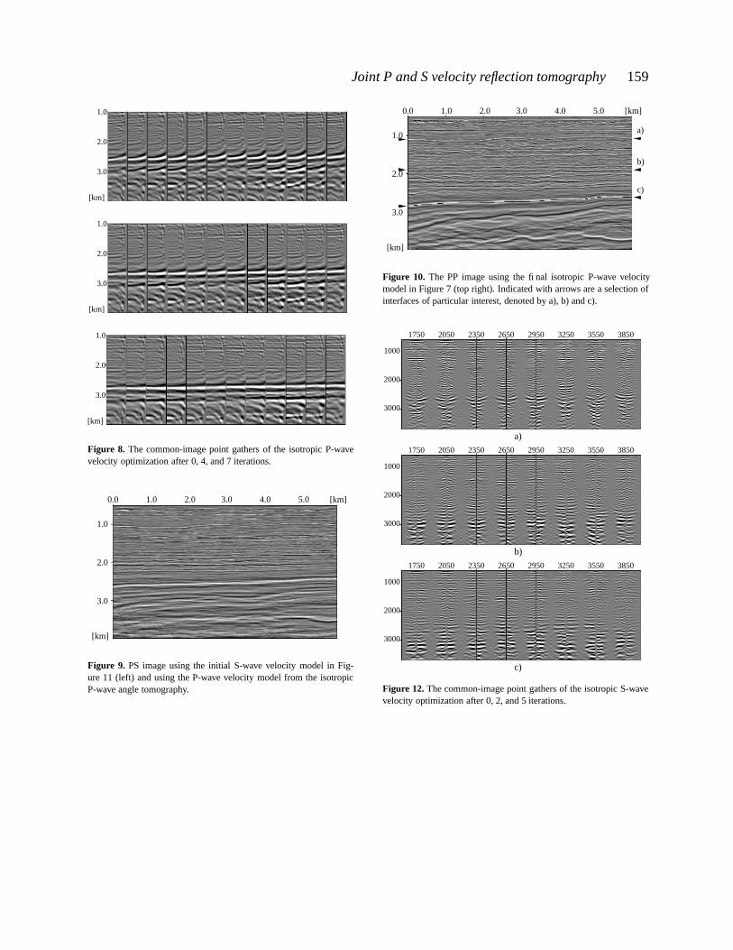
The 14 CIGs are sampled every 250 m from 1250 m on-wards. Each CIG is sampled every 0.5 degrees up to 45 de-grees in incoming P-wave reflection angle. Figure 8 shows thea) starting, b) after 4 iterations and c) after 7 iterations (final)collection of CIGS in the optimization. The resulting velocitymodel and corresponding PP image are given in Figures 7 (topright) and 10, respectively. The optimization for the B-splinecoefficients was carried out in the final couple of iterations,but this showed little improvement in the misfit function. No-tice in particular the movement of the interface geometry inthe final velocity model Figure 7 (top right) as compared withthe initial one (top left).

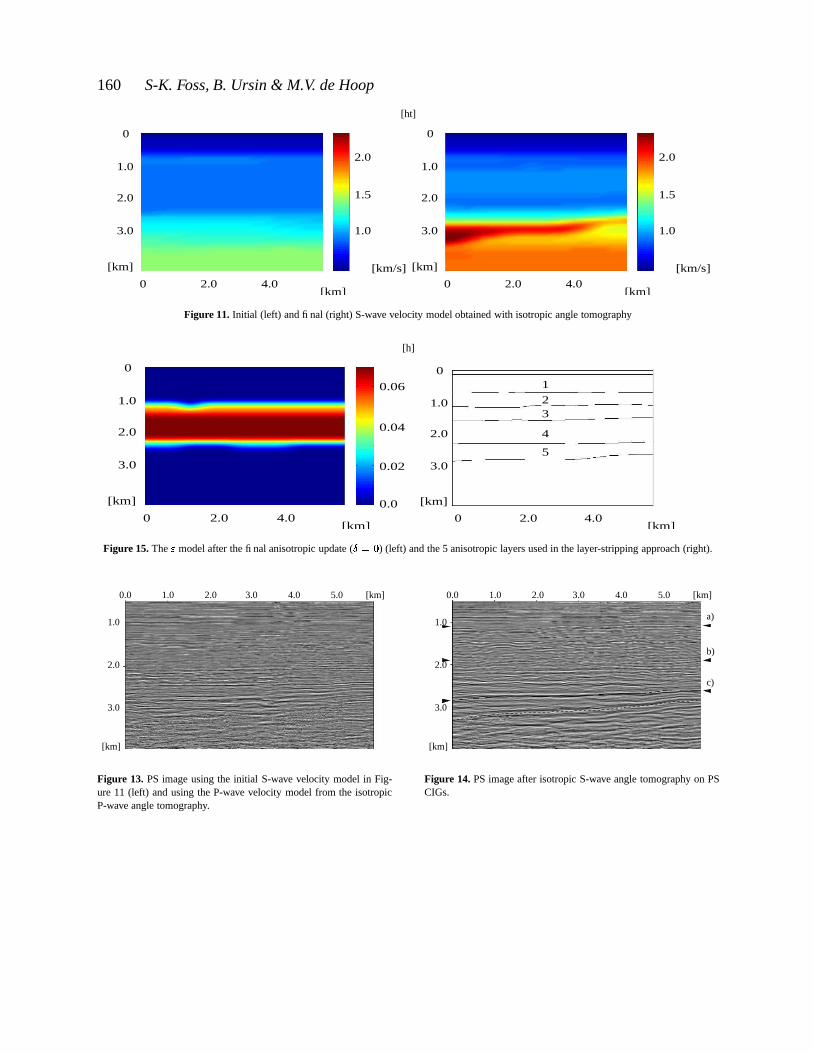
(ii) The initial S-wave velocity model is chosen naivelyby a fixed � � ( �� ratio for the entire model based on the fi-nal P-wave velocity, and is given in Figure 11 (left). The cor-responding PS image is given in Figure 13. The P-wave ve-locity model is considered reliable up to 45 degrees incom-


ing P-wave angle (which was the maximum angle used in theisotropic P-wave velocity analysis). We apply a tapered muteon the outgoing S-wave angles that through Snell’s law, aretied to incoming P-wave angles larger than 45 degrees. We use8 positive and negative CIGs,

��and

� Y , from surface po-sition 1750 m onwards with a 300 m horizontal spacing. Theinitial CIGS and the ones after the third and fifth iteration areshown in Figure 12 a), b) and c), respectively. The CIGs aredisplayed pairwise for the same horizontal position with thepositive image on the left and the negative image on the right,as explained in Figure 3. They are plotted as functions of out-going S-wave angle (contrary to convention) running from theindicated axis separating them, in the positive and negative di-rections. The S-wave angle ranges from 0.4 to 25 degrees.

(iii) The PS image resulting from the isotropic velocityanalysis is given in Figure 14. Superimposed are the arrowsand tracing of the main reflector ( c)) as found on the PP im-age, Figure 10. In the shallow part reflector a) of the PS imageoccurs slightly deeper than the corresponding reflector in thePP image (at the arrow). The depth discrepancy cannot be ex-plained by the CIGS in Figure 12c), which are uniform and in-dicate a fitting model according to our differential semblancein angle misfit measure. In the deeper parts the superimposedPP reflector c) seems to match a PS reflector, but the geolog-ically equivalent reflector on the PS image is indicated withthe dotted line. Thus under the isotropic assumption, the mi-grated, equivalent reflectors are several hundred meters apartin the PP and PS images.

To compute pure-mode SS traveltimes and slopes weidentify and pair several interfaces on both the PP and the PSimages, which are then map demigrated along the NIP rays toobtain the approximative SS traveltimes from equation (21).The key interfaces used are the three indicated with arrows inthe PP image (Figure 14).

(iv) In the process of co-depthing, the S-wave velocityis parameterized as in (28). The resulting depth-consistent PSimage is given in Figure 17 and is computed with the velocitymodel given in Figure 11 (right). The key reflectors in the PPand PS images are now at matching depths, but because ofthe isotropic assumption the PS CIGs show residual moveoutbehavior, again, as illustrated in Figure 16a). This concludesthe isotropic processing procedure.

(v) For the anisotropic processing we parameterize as(30) assuming the medium is TIV. There is no well-log infor-mation from wells intersecting our plane of consideration. Inaddition, the data has to be muted so that no large-offset dataare available for PP reflections from the shallow part of themodel. Hence, we set

� � � , as mentioned before. The start-ing value for the optimization is � � in the entire model.The CIGS are now sampled every 550 m in the horizontal di-rection starting at 1750 m; there are still 8 pairs of positive andnegative CIGS.

The gradient in the optimization is tapered at 700 m (andabove) and 2700 m (and below) based on ray coverage. Allparameters except are kept fixed at their values obtainedfrom isotropic velocity analysis. Figure 16 shows two sets ofCIGS. The first set, a), is the outcome of co-depthing (iv).

The shallow reflecting events are still quite uniform in theseCIGs, but, as seen in Figure 17, they have, in fact, moved inthe co-depthing step. This means that the velocity update in(iv) was not detectable by the differential semblance in anglemisfit function, because we have stayed in the range of the for-ward scattering operator. The final set of CIGS, Figure 16b),are optimized gathers after 2 iterations with . Most of thechange applies to the middle depth interval, between 1500 mand 2500 m. The resulting function and the correspondingimage are given in Figure 15 (left) and 18, respectively, wherethe indicators from the PP image (Figure 10) are again super-imposed. The geologically equivalent reflectors on the PP andPS images now appear to match in depth. However, below re-flector c), the PS image misses the structure clearly observablein the PP image. By investigating the set of PS CIGS in Fig-ure 16b) in this region, we observe misalignment or alignmentalong lines with large angles. Since the formation of causticsis unlikely here, we attribute these to wave constituents notmodeled by our 2.5-D scattering operator.

In Figure 19 we summarize the results by extracting asingle trace, at 3200 m horizontal distance, from the images inFigures 10 (step (i)), 14 (step (ii)), 17 (step (iv)) and 18 (step(v)). One can clearly observe the mistie in depth between thefirst two traces, the shift in depth from the second to the thirdtrace, and a reduction in oscillations from the third trace to thefourth trace.

Depth fidelity. In order to examine how the�-parameter

function influences results of the analysis proposed and carriedout above, we perform a joint PP and PS angle tomography, ina layer-stripping manner. We use the layering structure only,in the parametrization of

�and , and omit the contribution

from the splines. In addition, we limit the number of layersused to 5 as indicated in Figure 15 (right). Note that the inter-faces in this geometry form a subset of the set of interfaces inthe geometry in Figure 7 (bottom). The top layer (water) andthe bottom layer, below approximately 2700 m, are assumedisotropic. Isotropic parameters are taken from (i)-(ii)-(iv); thesampling of CIGs is the same as in step (v).

In addition to the differential semblance in angle misfitfunction we also include the sensitive semblance measure. Weintroduce the PP semblance-based misfit as

� �� $� , S ,� d�O e �� O ��* *

� �� >T6 � A�� 6 6 6 A �� 6 �� * � �� >T6 � A�� * � 6 6 6 A 6 � � 6 � � 6 � � � (37)

where the division in the integrand is a normalization ofeach CIG with its ‘energy’ (Chauris and Noble, 2001). Upondiscretizing the integrals,

� d�O e becomes the number of 6 andA values used, and

� �� O �� becomes the total number of CIGSused. Semblance optimization is here formulated as a mini-mization problem. We introduce in a similar manner the PS


semblance-based misfit,

� �� "� , S ,? �,� �d�O e � �� O ��

* *� �� >T6 � A�� 6 6 6 A �� 6 �� >T6 � A�� 6 6 6 A 6 �� 6 � � 6 � � J

4 ,� Yd@O e � Y�� O ��* *

� �� Y�@� �� > 6 � A�� 6 6 6 A �� 6 �� Y�� >T6 � A�� 6 6 6 A 6 � � 6 �� 6 �� where

� �d�O e and� �� O �� are defined as in (37) for the positive

CIGS and� Yd�O e and

� Y�� O �� for the negative CIGS.Figure 20 illustrates the shapes of the misfit for the five

different layers in a layer-stripping approach as function of and�. In the layer stripping approach, we use the optimal

� � � � values obtained in the layers above the layer in whichthe parameters are under investigation. Shown, by column, arethe semblance misfits for PS, PP (equations (??) and (37)),their normalized sum, and our joint PP, PS differential sem-blance in angle misfit ( � � � � � � , , � � � ). The PP andPS semblance functions are plotted on the same scale. In thePS semblance plot, the apparent valley at a 45 degree angleis governed by � S � � as in equation (33). This indicates thefeasibility of detecting anisotropy in the PS CIGS, without dis-criminating between the two parameters. In the PP semblanceplot we are unable to observe significant change in the value ofthe misfit function with changing anisotropy. This is expectedas the data offsets are not sufficiently large for the shallow partof the model because of the aforementioned mute.

In the joint PP, PS semblance and joint PP, PS differentialsemblance in angle misfit plots, the lines

� �Z� and

S & � � S &� � (38)

are drawn, where& and

&�are optimal values for � and

�in

each layer, and can be found in Table 1. In the first three layersthe values are chosen using the PS semblance plot only, with� � � , since there is not enough resolution in

�. In layers 4

and 5 we use the joint PP, PS semblance plots. In these layersvalues for and

�can be resolved by locating the semblance

misfit minimum after analyzing the joint PP, PS differentialsemblance in angle misfit function first. In the deepest layer, athreshold on the differential semblance in angle misfit functionlimits the region where the semblance misfit minimum is to befound, and thus enables us to discriminate between the twoapparent minima in the semblance misfit function.

In the calculations we use a fixed depth window of theCIGs. This implies, for example, that if

�becomes too nega-

tive, an event can move out of this depth window and hence nolonger contributes to the misfit.

The final PP and PS CIGs for the& and

&�values in Ta-

ble 1 are shown in Figure 21. The corresponding images aregiven in Figures 22 and 23 in depth and in two-way PP time(obtained by depth-to-time conversion using the P-wave ve-locities from (i)) in Figures 24 and 25. The images in the latter

layer �� 1 0.035 0.0

2 0.0 0.0

3 0.02 0.0

4 0.09 -0.04

5 -0.02 -0.02

Table 1. Anisotropic parameter values resulting from layer stripping.

two figures correlate very well. For comparison, the initial PPimage obtained in (i) is also converted to two-way PP time inFigure 26.

7 DISCUSSION AND CONCLUSION

We have presented a reflection tomographic or MVA ap-proach to obtain depth-consistent PP and PS images by mak-ing use of a differential semblance in angle measures and map(de)migration, enabling automatic measurement of any mistiein depth. This involves an extension of differential semblancein angle to converted waves, as well as the development ofa co-depthing measure. The co-depthing procedure is derivedfrom the zero scattering angle case of Grechka and Tsvankin’s‘PP+PS=SS’ concept. When the velocity model is far from thetrue model, or when there is a significant inconsistency be-tween the models governing the P-wave leg and the S-waveleg of the PS scattering event, the approximation we make inthe ‘PP+PS=SS’ concept deteriorates. Also, the current co-depthing procedure, based on zero scattering angle, fails toapply in the presence of caustics. Then the co-depthing proce-dure can be refined by using the aforementioned ‘PP+PS=SS’approach to compute prestack SS traveltimes and slopes, andmaking use of finite-offset map (de)migration.

Perhaps one would expect that by first estimating a P-wave velocity model from PP reflections and then an S-wavevelocity model from PS reflections would guarantee consis-tency in depth between PP and PS images, since the mode-converted wave is tied to the P wave. The field data exampleillustrates that this is not the case: The difference in depths canbe several hundred meters even if the differential semblance inangle measure, through uniform CIGS, indicate a model fittingboth the PP and PS scattering events.

The tying of the PP and PS events forces us to takeanisotropy into account; this has been observed by severalauthors, see for example Artola et al. (2003). We developedan approach derived from joint PP and PS angle tomography,consisting of five steps, for carrying out MVA. We estimateda compressional- and shear-wave velocity model based on aquasi-TIV medium (Thomsen’s

� � � ) assumption. We alsosucceeded in estimating

�separately from , with a degree of

uncertainty, in part of the model; in this estimation we madeadditional use of a semblance measure applied to the PP and


PS CIGs. As to be expected, the best resolved parameter com-bination from PS angle tomography is S � .

The , � parameter estimation was carried out in a layer-stripping manner. The estimates for are significantly differ-ent from those obtained by the automatic global search for aquasi-TIV medium. This shows that our procedure and strat-egy cannot lead to uniqueness of the reflection tomographyproblem.

Our method shows the potential to achieve depth consis-tency and uniform CIGs at the same time. It relies heavily onthe ability to identify, interpret, and pair interfaces on the PPand PS images. The success of this depends on whether PSimages of sufficient quality can be generated to begin with. Itcan be argued that the current field data example could havebeen solved by a less sophisticated method, such as one basedon the generalized Dix approach. Our method, however, ex-tends far beyond the cases where the generalized Dix equationapplies.

One of the potential applications of reflection tomog-raphy is pore pressure prediction (Sayers et al., 2004). Ourmethod can not only provide P-wave velocity models at ahigher spatial resolution than can be obtained by hyperbolicmoveout or other convential velocity analyses, it can also yieldan improved estimate of the local �� ( �� ratio.

ACKNOWLEDGMENTS

The authors thank Statoil for the North Sea data set and BørgeArntsen for the data handling. In addition, they thank AndersSollid, Statoil for many helpful discussions. Stig-Kyrre Fosswould like to thank the URE-project at NTNU, Norway forfinancial support.

8 References

Al-Yahya, K., 1989, Velocity analysis by iterative profile mi-gration: Geophysics, 54, 718–729.

Alerini, M., Le Begat, S., Lambare, G., and Baina, R., 2002,2D PP- and PS-stereotomography for a multicomponentdataset: Proceedings 72th Ann. Internat. Mtg., Soc. Explor.Geophys., pages 838–841.

Alkhalifah, T., and Tsvankin, I., 1995, Velocity analysis fortransversely isotropic media: Geophysics, 60, 1550–1566.

Artola, F., Da Fontoura, S., Leiderman, R., and Silva, M.,2003, P-S conversion point in anisotropic media - errorsdue to isotropic considerations: Proceedings 64th Mtg. Eur.Assn. Geosci. Eng., pages D–12.

Audebert, F., Granger, P.-Y., Gerea, C., and Herrenschmidt,A., 2001, Can joint pp and ps velocity analysis manageto corner

�, the anisotropic depthing parameter?: Proceed-

ings 69th Ann. Internat. Mtg., Soc. Explor. Geophys., pages145–148.

Billette, F., and Lambare, G., 1998, Velocity macro-model es-timation from seismic reflection data by stereotomography:Geophys. J. Int., 135, 671–690.

Brandsberg-Dahl, S., de Hoop, M. V., and Ursin, B., 1999, Ve-locity analysis in the common scattering-angle/azimuth do-main: Proceedings 69th Ann. Internat. Mtg., Soc. Explor.Geophys., pages 1222–1223.

Brandsberg-Dahl, S., de Hoop, M. V., and Ursin, B., 2003a,Focusing in dip and AVA compensation on scattering-angle/azimuth gathers: Geophysics, 68, 232–254.

——– 2003b, Seismic velocity analysis in the scattering an-gle/azimuth domain: Geophysical Prospecting, 51, 295–314.

Broto, K., Ehinger, A., Kommedal, J. H., and Folstad, P. G.,2003, Anisotropic traveltime tomography for depth consis-tent imaging of pp and ps data: The Leading Edge, 22, 114–119.

Bube, K. P., and Meadows, M. A., 1999, The null space of agenerally anisotropic medium in linearized surface reflec-tion tomography: Geophys, J. Int., 139, 9–50.

Bube, K. P., Langan, R. T., and Nemeth, T., 2002, On the ve-locity vs. depth ambiguity in limited-aperture reflection to-mography: Proceedings 72th Ann. Internat. Mtg., Soc. Ex-plor. Geophys., pages 834–837.

Bube, K. P., 1995, Uniqueness of reflector depths and charac-terization of the slowness null space in linearized seismicreflection tomography: SIAM Journal on Applied Mathe-matics, 55, 255–266.

Burridge, R., de Hoop, M. V., Miller, D., and Spencer, C.,1998, Multiparameter inversion in anisotropic media: Geo-physical Journal International, 134, 757–777.

Carcione, J. M., 2001, Wave fields in real media: Wave prop-agation in anisotropic, anelastic and porous media: , Perga-mon.

Cerveny, V., 2001, Seismic ray theory: , Cambridge UniversityPress.

Chauris, H., and Noble, M., 2001, Two-dimensional velocitymacro model estimation from seismic reflection data by lo-cal differential semblance optimization: application to syn-thetic and real data sets: Geophys. J. Int., 144, 14–26.

de Boor, C., 1978, A practical guide to splines: , Springer, NewYork.

de Hoop, M. V., and Bleistein, N., 1997, Generalized Radontransform inversions for reflectivity in anisotropic elasticmedia: Inverse Problems, 13, 669–690.

de Hoop, M. V., Burridge, R., Spencer, C., and Miller, D.,1994, Generalized Radon transform amplitude versus an-gle (GRT/AVA) migration/inversion in anisotropic media:Proceedings SPIE 2301, pages 15–27.

de Hoop, M. V., Spencer, C., and Burridge, R., 1999, The re-solving power of seismic amplitude data: An anisotropicinversion/migration approach: Geophysics, 64, 852–873.

Douma, H., and de Hoop, M., 2003, Closed-form expres-sions for map time-migration in vti media and applicabilityof map depth-migration in the presence of caustics: Geo-physics, submitted.

Farra, V., and Madariaga, R., 1987, Seismic waveform mod-eling in heterogeneous media by ray perturbation theory:Journal of Geophysical Research, 92, 2697–2712.

Fomel, S., 1997, Velocity continuation and the anatomy of


residual prestack migration: Proceedings 67th Ann. Inter-nat. Mtg. Soc. of Expl. Geophys., pages 1762–1765.

Foss, S. K., and Ursin, B., 2003, 2.5-D modeling, inversionand angle migration in anisotropic elastic media: Geophys-ical Prospecting, Accepted.

Foss, S. K., de Hoop, M., and Ursin, B., 2003a, Linearized 2.5-D parameter imaging-inversion in anisotropic elasic media:Geophys. J. Int., submitted.

——– 2003b, A practical approach to automated pp angle to-mography: EAGE / SEG summer research workshop in Tri-este.

Gill, P. E., Murray, W., and H., W. M., 1981, Practical opti-mization: , Academic Press.

Gjoystdal, H., and Ursin, B., 1981, Inversion of reflectiontimes in three-dimensions: Geophysics, 46, 972–983.

Grechka, V., and Tsvankin, I., 2002a, The joint nonhyperbolicmoveout inversion of pp and ps data in vti media: Geo-physics, 67, 1929–1932.

——– 2002b, Pp + ps = ss: Geophysics, 67, 1961–1971.Grechka, V., Pech, A., and Tsvankin, I., 2002, Multi-

component stacking-velocity tomography for transverselyisotropic media: Geophysics, 67, 1564–1574.

Herrenschmidt, A., Granger, P.-Y., Audebert, F., Gerea, C.,Etienne, G., Stopin, A., Alerini, M., Le Begat, S., Lam-bare, G., Berthet, P., Nebieridze, S., and Boelle, J.-L., 2001,Comparison of different strategies for velocity model build-ing and imaging of pp and ps real data: The Leading Edge,20, 984–995.

Hubral, P., and Krey, T., 1980, Interval velocities from seismicreflection time measurements: , Soc. of Expl. Geophys.

Iversen, E., Gjøystdal, H., and Hansen, J. O., 2000, Prestackmap migration an engine for parameter estimation in timedia: Proceedings 70th Ann. Internat. Mtg., Soc. Explor.Geophys., pages 1004–1007.

Iversen, E., 2001, First-order perturbation theory for seismicisochrones: Studia geophysica et geodaetica, 45, 394–444.

Kleyn, A. H., 1977, On the migration of reflection-time con-tour maps: Geophys. Prosp., 25, 125–140.

Plessix, R.-E., ten Kroode, F., and Mulder, W., 2000, Auto-matic crosswell tomography by differential semblance op-timization: theory and gradient computation: GeophysicalProspecting, 48, 913–935.

Sayers, C. M., Smit, T. J. H., van Eden, C., Wervelman,R., Bachmann, B., Fitts, T., Bingham, J., McLachlan, K.,Hooyman, P., Noeth, S., and Mandhiri, D., 2004, Use ofreflection tomography to predict pore pressure in overpres-sured reservoir sands: 74th Ann. Internat. Mtg., Soc. Ex-plor. Geophys., Expanded Abstracts, –.

Sollid, A., 2000, Imaging of ocean bottom seismic data: Ph.D.thesis, Norwegian University of Science and Technology,Trondheim.

Stolk, C. C., and de Hoop, M. V., 2002, Microlocal analy-sis of seismic inverse scattering in anisotropic elastic me-dia: Communications in Pure and Applied Mathematics,55, 261–301.

Stolk, C. C., and de Hoop, M. V., 2004, Seismic inverse scat-tering in the downward continuation approach: SIAM J.

Appl. Math.Stolk, C. C., 2002, Microlocal analysis of the scattering angle

transform: Comm. PDE, 27, 1879–1900.Stopin, A., and Ehinger, A., 2001, Joint pp ps tomographic

inversion of the mahogany 2-d-4-c obc seismic data: Pro-ceedings 71th Ann. Internat. Mtg., Soc. Explor. Geophys.,pages 837–840.

Stork, C., and Clayton, R. W., 1986, Analysis of the resolutionbetween ambiguous velocity and reflector position for trav-eltime tomography: Proceedings 56th Ann. Internat. Mtg.,Soc. Explor. Geophys., pages 545–550.

Symes, W., and Carazzone, J., 1991, Velocity inversion bydifferential semblance optimization: Geophysics, 56, 654–663.

Symes, W., 1991, A differential semblance algorithm for theinverse problem of reflection seismology: Computers Math.Applic., 22, 147–178.

Symes, W., All stationary points of differential semblance areasymptotic global minimizers: layered acoustics:, Rice In-version Project, Annual report, 2000.

Taner, M. T., and Koehler, F., 1969, Velocity spectra - Digitalcomputer derivation and applications of velocity functions:Geophysics, 34, 859–881.

Thomsen, L., 1986, Weak elastic anisotropy: Geophysics, 51,1954–1966.

Thomsen, L., 1999, Converted-wave reflection seismologyover inhomogeneous, anisotropic media: Geophysics, 64,678–690.

Tsvankin, I., and Grechka, V., 2002, 3D description and in-version of reflection moveout of PS-waves in anisotropicmedia: Geoph. Prosp., 50, 301–316.

Tygel, M., Schleicher, J., and Hubral, P., 1994, Pulse distortionin depth migration: Geophysics, 59, 1561–1569.

Ursin, B., 2003, Parameter inversion and angle migration inanisotropic elastic media: Geophysics, Accepted.

Versteeg, R. J., 1993, Sensitivity of prestack depth migrationto the velocity model: Geophysics, 58, 873–882.

Whitcombe, D. N., 1994, Fast model building using demigra-tion and single-step ray migration: Geophysics, 59, 439–449.

Yilmaz, O., 1987, Seismic data processing: vol. 2 of Investiga-tions in Geophysics, Society of Exploration Geophysicists,Tulsa.


�

�

��

��

��

��

�

��

� ��

��

showpage

Figure 1. Geometry of rays connecting the imaging point with the source and the receiver; an illustration of map (de)migration.

�

�

� � ��

� � ��

� � ��

��

�

��

� � ��

� �

Figure 2. The differential semblance misfit function in angle is differentiated keeping the image point, scattering angle, azimuth and migration dipfixed. Dotted lines indicate perturbed rays.


��

��

��

��

Figure 3. Positive and negative PS CIGS, � �� and � Y�� . The arrows indicate the ray directions in the two reflection events. The solid and dashedcurves are the P- and S-wave legs, respectively, of the different events.

��

� �

�

� ��

Figure 4. Two normal-incidence-point (NIP) rays for the P and S wave from the subsurface point .

��

�

��

� ��

� ��

Figure 5. Mapping of the NIP reflection traveltime function and slopes to reflector depths and dips, given a velocity model ! and ! .


� � �

PP image

PS image�

�

Figure 6. The reflector point imaged at and from PP and PS reflection data, respectively, resulting from an inconsistent background model.Indicated are NIP rays from the two reflector points to the acquisition surface.

0

0

[km]

[km]

[km/s]

4.0

2.0

1.0

2.0

3.0

3.0

4.02.0 0

0

[km]

[km]

[km/s]

4.0

2.0

1.0

2.0

3.0

3.0

4.02.0

0

0

[km]

[km]

1.0

2.0

4.02.0

3.0

Figure 7. Initial (top left) and final (top right) P-wave velocity model from isotropic angle tomography, with the final interface geometry (bottom).


[km]

3.0

2.0

1.0

[km]

3.0

2.0

1.0

[km]

3.0

2.0

1.0

Figure 8. The common-image point gathers of the isotropic P-wavevelocity optimization after 0, 4, and 7 iterations.

1.0

2.0

3.0

0.0 1.0 2.0 3.0 4.0 5.0

[km]

[km]

Figure 9. PS image using the initial S-wave velocity model in Fig-ure 11 (left) and using the P-wave velocity model from the isotropicP-wave angle tomography.

1.0

2.0

3.0

0.0 1.0 2.0 3.0 4.0 5.0

[km]

[km]

a)

b)

c)

Figure 10. The PP image using the final isotropic P-wave velocitymodel in Figure 7 (top right). Indicated with arrows are a selection ofinterfaces of particular interest, denoted by a), b) and c).

1000

2000

3000

a)

2050 29501750 2350 2650 3250 3550 3850

1000

2000

3000

1750 2050 2350 2650 2950 3550 3850

b)

3250

1000

2000

3000

1750 2050 2350 2650 2950 3250 3550 3850

c)

Figure 12. The common-image point gathers of the isotropic S-wavevelocity optimization after 0, 2, and 5 iterations.


[ht]

0

0

[km]

[km]

[km/s]

1.0

2.0

3.0

4.02.0

1.0

1.5

2.0

0

0

[km]

[km]

[km/s]

1.0

2.0

3.0

4.02.0

1.0

1.5

2.0

Figure 11. Initial (left) and final (right) S-wave velocity model obtained with isotropic angle tomography

[h]

0

0

[km]

[km]

1.0

2.0

3.0

4.02.00.0

0.02

0.04

0.06

0

0

[km]

[km]

1.0

2.0

4.02.0

3.0

1

3

4

5

2

Figure 15. The � model after the final anisotropic update (� �� ) (left) and the 5 anisotropic layers used in the layer-stripping approach (right).

1.0

2.0

3.0

0.0 1.0 2.0 3.0 4.0 5.0

[km]

[km]

Figure 13. PS image using the initial S-wave velocity model in Fig-ure 11 (left) and using the P-wave velocity model from the isotropicP-wave angle tomography.

1.0

2.0

3.0

0.0 1.0 2.0 3.0 4.0 5.0

[km]

[km]

a)

b)

c)

Figure 14. PS image after isotropic S-wave angle tomography on PSCIGs.


1000

2000

3000

750 1300 1850 2400 2950 3500 4050 4600

a)

1000

2000

3000

750 1300 2400 2950 3500 4050 4600

b)

1850

Figure 16. The common-image point gathers of the angle tomographyin � after a) 0 and b) 2 iterations.

1.0

2.0

3.0

0.0 1.0 2.0 3.0 4.0 5.0

[km]

[km]

a)

b)

c)

Figure 17. PS image after isotropic co-depthing.

1.0

2.0

0.0 1.0 2.0 3.0 4.0 5.0

[km]

[km]

3.0

a)

b)

c)

Figure 18. PS image after quasi-TIV parameter update (� �� ).

3.0

10 14 17 18

c)

2.5

3.5[km]

3.2 km

Figure 19. A single trace, at 3200 m horizontal distance, from theimages in Figures 10 (step (i)), 14 (step (ii)), 17 (step (iv)) and 18(step (v)).

1

3

4

5

2

Figure 20. Contour plots for anisotropic layers 1-5 (vertical direc-tion) and misfit plots for PS, PP and PP+PS semblance, and differ-ential semblance in angle for PP+PS. The semblance plots are givenby equations (37) and (??), formulated as minimization problems forcomparison with the differential semblance misfit function.


[km]

[m]2050 2350 2650 2950 3250 3550 3850

1.0

2.0

3.0

PP

1750

[km]

[m]2050 2350 2650 2950 3250 3550 3850

1.0

2.0

3.0

PS

1750

Figure 21. Final PP and PS CIGS after anisotropic model update ob-tained following a layer-stripping approach.

1.0

2.0

3.0

0.0 1.0 2.0 3.0 4.0 5.0

[km]

[km]

a)

b)

c)

Figure 22. PP image using the anisotropic parameters obtained fromthe layer stripping.

1.0

2.0

3.0

0.0 1.0 2.0 3.0 4.0 5.0

[km]

[km]

a)

b)

c)

Figure 23. PS image using the anisotropic parameters obtained fromthe layer stripping.

[km]

1.0

2.0

[s]

0.0 1.0 2.0 3.0 4.0 5.0

Figure 24. PP image using the anisotropic parameters obtained fromthe layer stripping, in two-way PP time.

[km]

1.0

2.0

[s]

0.0 1.0 2.0 3.0 4.0 5.0

Figure 25. PP image using the anisotropic parameters obtained fromthe layer stripping, in two-way PP time.


[km]

1.0

2.0

[s]

0.0 1.0 2.0 3.0 4.0 5.0

Figure 26. The initial PP image obtained in (i) (same as in Figure 9),in two-way PP time.

joint p- and s-wave velocity reﬂection tomography using pp

Documents